Author: Richard B. Langley

  • Innovation: Evil Waveforms

    Innovation: Evil Waveforms

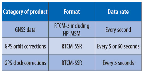
    Generating Distorted GNSS Signals Using a Signal Simulator

    By Mathieu Raimondi, Eric Sénant, Charles Fernet, Raphaël Pons, Hanaa Al Bitar, Francisco Amarillo Fernández, and Marc Weyer

    GPS World photo
    INNOVATION INSIGHTS by Richard Langley

    INTEGRITY.  It is one of the most desirable personality traits. It is the characteristic of truth and fair dealing, of honesty and sincerity. The word also can be applied to systems and actions with a meaning of soundness or being whole or undivided. This latter definition is clear when we consider that the word integrity comes from the Latin word integer, meaning untouched, intact, entire — the same origin as that for the integers in mathematics: whole numbers without a fractional or decimal component.

    Integrity is perhaps the most important requirement of any navigation system (along with accuracy, availability, and continuity). It characterizes a system’s ability to provide a timely warning when it fails to meet its stated accuracy. If it does not, we have an integrity failure and the possibility of conveying hazardously misleading information. GPS has built into it various checks and balances to ensure a fairly high level of integrity. However, GPS integrity failures have occasionally occurred.

    One of these was in 1990 when SVN19, a GPS Block II satellite operating as PRN19, suffered a hardware chain failure, which caused it to transmit an anomalous waveform. There was carrier leakage on the L1 signal spectrum. Receivers continued to acquire and process the SVN19 signals, oblivious to the fact that the signal distortion resulted in position errors of three to eight meters. Errors of this magnitude would normally go unnoticed by most users, and the significance of the failure wasn’t clear until March 1993 during some field tests of differential navigation for aided landings being conducted by the Federal Aviation Administration. The anomaly became known as the “evil waveform.”

    (I’m not sure who first came up with this moniker for the anomaly. Perhaps it was the folks at Stanford University who have worked closely with the FAA in its aircraft navigation research. The term has even made it into popular culture. The Japanese drone-metal rock band, Boris, released an album in 2005 titled Dronevil. One of the cuts on the album is “Evil Wave Form.” And if drone metal is not your cup of tea, you will find the title quite appropriate.) Other types of GPS evil waveforms are possible, and there is the potential for such waveforms to also occur in the signals of other global navigation satellite systems. It is important to fully understand the implications of these potential signal anomalies. In this month’s column, our authors discuss a set of GPS and Galileo evil-waveform experiments they have carried out with an advanced GNSS RF signal simulator. Their results will help to benchmark the effects of distorted signals and perhaps lead to improvements in GNSS signal integrity.


    “Innovation” is a regular feature that discusses advances in GPS technology andits applications as well as the fundamentals of GPS positioning. The column is coordinated by Richard Langley of the Department of Geodesy and Geomatics Engineering, University of New Brunswick. He welcomes comments and topic ideas.

    GNSS signal integrity is a high priority for safety applications. Being able to position oneself is useful only if this position is delivered with a maximum level of confidence. In 1993, a distortion on the signals of GPS satellite SVN19/PRN19, referred to as an “evil waveform,” was observed. This signal distortion induced positioning errors of several meters, hence questioning GPS signal integrity. Such events, when they occur, should be accounted for or, at least, detected.

    Since then, the observed distortions have been modeled for GPS signals, and their theoretical effects on positioning performance have been studied through simulations. More recently, the models have been extended to modernized GNSS signals, and their impact on the correlation functions and the range measurements have been studied using numerical simulations. This article shows, for the first time, the impact of such distortions on modernized GNSS signals, and more particularly on those of Galileo, through the use of RF simulations. Our multi-constellation simulator, Navys, was used for all of the simulations.

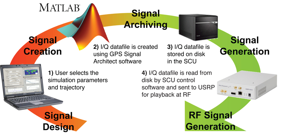
    These simulations are mainly based on two types of scenarios: a first scenario, referred to as a static scenario, where Navys is configured to generate two signals (GPS L1C/A or Galileo E1) using two separate RF channels. One of these signals is fault free and used as the reference signal, and the other is affected by either an A- or B-type evil waveform (EW) distortion (these two types are described in a latter section).

    The second type of scenario, referred to as a dynamic scenario, uses only one RF channel. The generated signal is fault free in the first part of the simulation, and affected by either an A- or B-type EW distortion in the second part of the scenario. Each part of the scenario lasts approximately one minute.

    All of the studied scenarios consider a stationary satellite position over time, hence a constant signal amplitude and propagation delay for the duration of the complete scenario.

    Navys Simulator

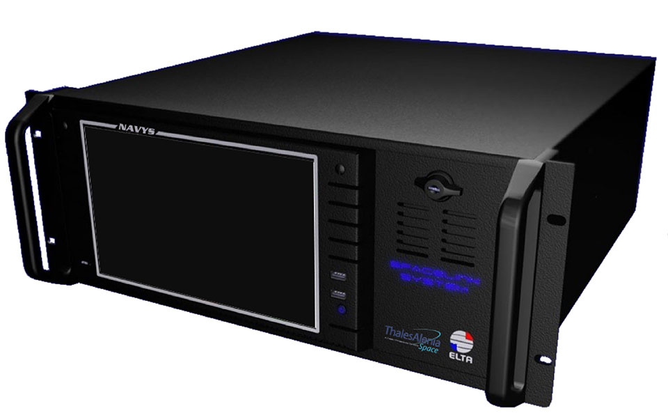
    The first versions of Navys were specified and funded by Centre National d’Etudes Spatiales or CNES, the French space agency. The latest evolutions were funded by the European Space Agency and Thales Alenia Space France (TAS-F). Today, Navys is a product whose specifications and ownership are controled by TAS-F. It is made up of two components: the hardware part, developed by ELTA, Toulouse, driven by a software part, developed by TAS-F.

    The Navys simulator can be configured to simulate GNSS constellations, but also propagation channel effects. The latter include relative emitter-receiver dynamics, the Sagnac effect, multipath, and troposphere and ionosphere effects. Both ground- and space-based receivers may be considered.

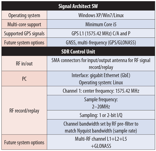
    GNSS Signal Generation Capabilities. Navys is a multi-constellation simulator capable of generating all existing and upcoming GNSS signals. Up to now, its GPS and Galileo signal-generation capabilities and performances have been experienced and demonstrated. The simulator, which has a generation capacity of 16 different signals at the same time over the entire L band, has already been successfully tested with GPS L1 C/A, L1C, L5, and Galileo E1 and E5 receivers.

    Evil Waveform Emulation Capabilities. In the frame of the ESA Integrity Determination Unit project, Navys has been upgraded to be capable of generating the signal distortions that were observed in 1993 on the signals from GPS satellite SVN19/PRN19. Two models have been developed from the observations of the distorted signals.

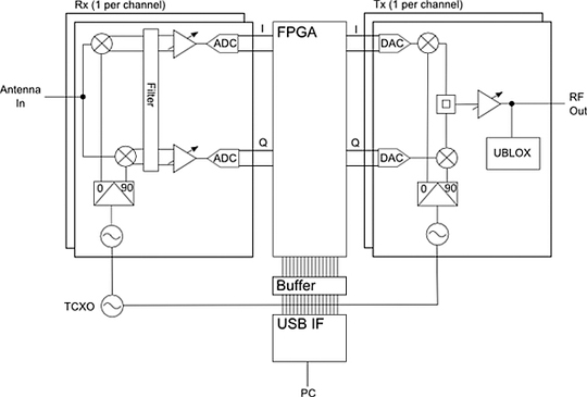
    The first one, referred to as Evil Waveform type A (EWFA), is associated with a digital distortion, which modifies the duration of the GPS C/A code chips, as shown in FIGURE 1. A lead/lag of the pseudorandom noise code chips is introduced. The +1 and –1 state durations are no longer equal, and the result is a distortion of the correlation function, inducing a bias in the pseudorange measurement equal to half the difference in the durations. This model, based on GPS L1 C/A-code observations, has been extended to modernized GNSS signals, such as those of Galileo (see Further Reading). In Navys, type A EWF generation is applied by introducing an asymmetry in the code chip durations, whether the signal is modulated by binary phase shift keying (BPSK), binary offset carrier (BOC), or composite BOC (CBOC).

    FIGURE 1. Theoretical L1 C/A code-chip waveforms in the presence of an EWFA (top) and EWFB (bottom).
    FIGURE 1. Theoretical L1 C/A code-chip waveforms in the presence of an EWFA (top) and EWFB (bottom).

    The second model, referred to as Evil Waveform type B (EWFB) is associated with an analog distortion equivalent to a second-order filter, described by a resonance frequency (fd) and a damping factor (σ), as depicted in Figure 1. This failure results in correlation function distortions different from those induced by EWFA, but which also induces a bias in the pseudorange measurement. This bias depends upon the characteristics (resonance frequency, damping factor) of the filter. In Navys, an infinite impulse response (IIR) filter is implemented to simulate the EWFB threat. The filter has six coefficients (three in the numerator and three in the denominator of its transfer function). Hence, it appears that Navys can generate third order EWF type B threats, which is one order higher that the second order threats considered by the civil aviation community. Navys is specified to generate type B EWF with less than 5 percent root-mean-square  (RMS) error between the EWF module output and the theoretical model. During validation activities, a typical value of 2 percent RMS error was measured. This EWF simulation function is totally independent of the generated GNSS signals, and can be applied to any of them, whatever its carrier frequency or modulation.

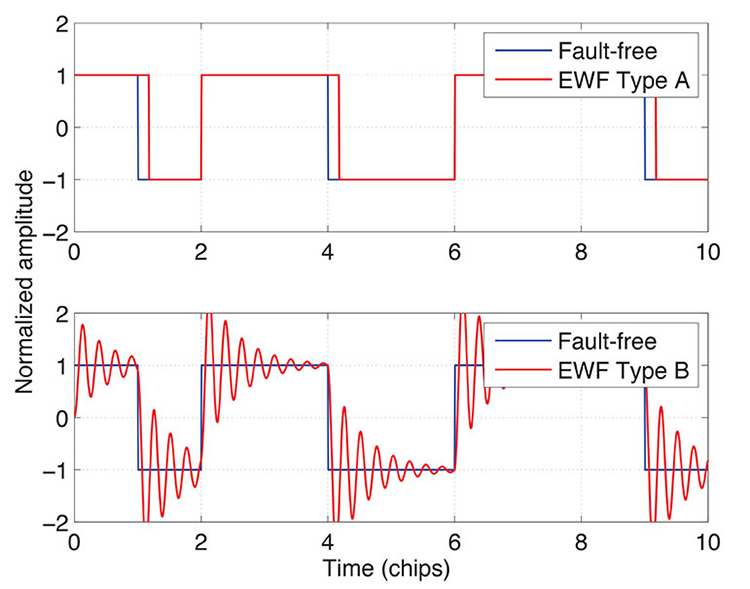
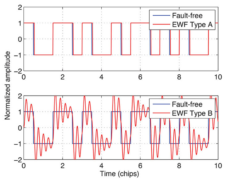
    It is important to note that such signal distortions may be generated on the fly — that is, while a scenario is running. FIGURE 2 gives an example of the application of such threat models on the Galileo E1 BOC signal using a Matlab theoretical model.
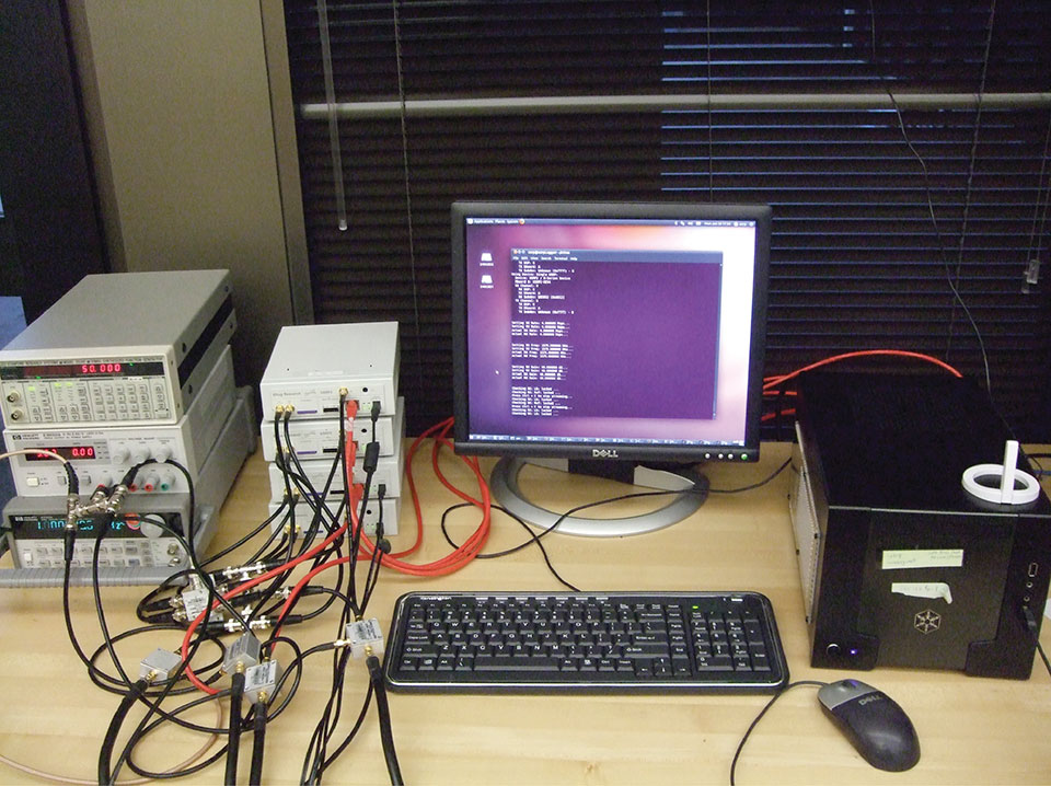
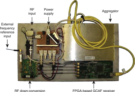
    FIGURE 2. Theoretical E1 C code-chip waveforms in the presence of an EWFA (top) and EWFB (bottom).
    FIGURE 2. Theoretical E1 C code-chip waveforms in the presence of an EWFA (top) and EWFB (bottom).

    GEMS Description

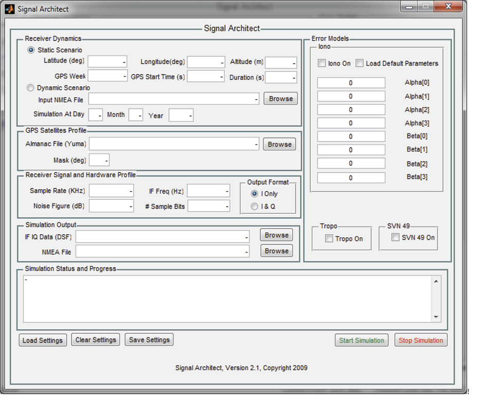
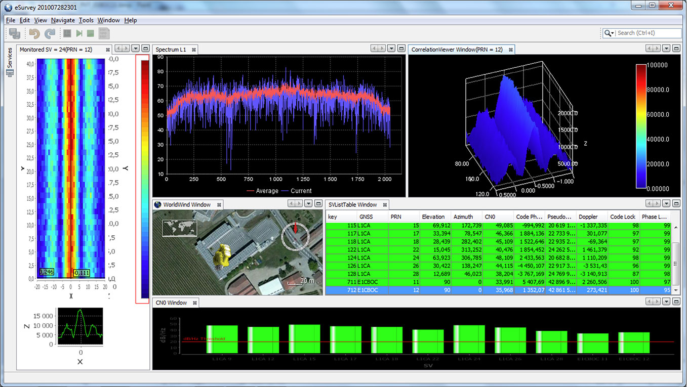
    GEMS stands for GNSS Environment Monitoring Station. It is a software-based solution developed by Thales Alenia Space aiming at assessing the quality of GNSS measurements. GEMS is composed of a signal processing module featuring error identification and characterization functions, called GEA, as well as a complete graphical user interface (see online version of this article for an example screenshot) and database management.

    The GEA module embeds the entire signal processing function suite required to build all the GNSS observables often used for signal quality monitoring (SQM). The GEA module is a set of C/C++ software routines based on innovative-graphics-processing-unit (GPU) parallel computing, allowing the processing of a large quantity of data very quickly. It can operate seamlessly on a desktop or a laptop computer while adjusting its processing capabilities to the processing power made available by the platform on which it is installed. The GEA signal-processing module is multi-channel, multi-constellation, and supports both real-time- and post-processing of GNSS samples produced by an RF front end.

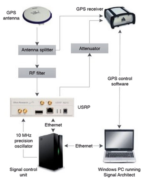
    GEMS, which is compatible with many RF front ends, was used with a commercial GNSS data-acquisition system. The equipment was configured to acquire GNSS signals at the L1 frequency, with a sampling rate of 25 MHz. The digitized signals were provided in real time to GEMS using a USB link.

    From the acquired samples, GEMS performed signal acquisition and tracking, autocorrelation function (ACF) calculation and display, and C/N0 measurements. All these figures of merit were then logged in text files.

    EWF Observation

    Several experiments were carried out using both static and kinematic scenarios with GPS and Galileo signals.

    GPS L1 C/A. The first experiment was intended to validate Navys’ capability of generating state-of-the-art EWFs on GPS L1 C/A signals. It aimed at verifying that the distortion models largely characterized in the literature for the GPS L1 C/A are correctly emulated by Navys.

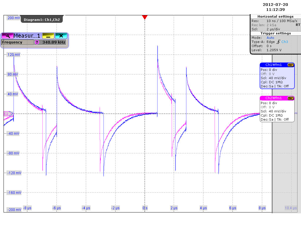
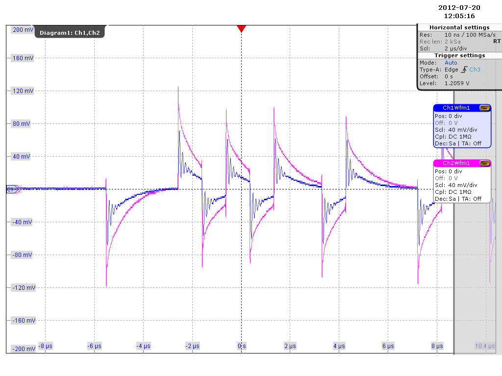
    EWFA, static scenario. In this scenario, Navys is configured to generate two GPS L1 C/A signals using two separate RF channels. The same PRN code was used on both channels, and a numerical frequency transposition was carried out to translate the signals to baseband. One signal was affected by a type A EWF, with a lag of 171 nanoseconds, and the other one was EWF free. Next, its amplified output was plugged into an oscilloscope. The EWFA effect is easily seen as the faulty signal falling edge occurs later than the EWF-free signal, while their rising edges are still synchronous. However, the PRN code chips are distorted from their theoretical versions as the Navys integrates a second-order high pass filter at its output, meant to avoid unwanted DC emissions. The faulty signal falling edge should occur approximately 0.17 microseconds later than the EWF-free signal falling edge.

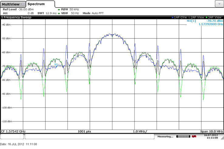
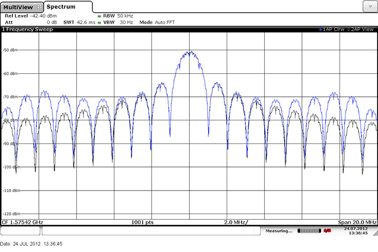
    A spectrum analyzer was used to verify, from a spectral point of view, that the EWFA generation feature of Navys was correct. For this experiment, Navys was configured to generate a GPS L1 C/A signal at the L1 frequency, and Navys output was plugged into the spectrum analyzer input. Three different GPS L1 C/A signals are included: the spectrum of an EWF-free signal, the spectrum of a signal affected by an EWF type A, where the lag is set to 41.1 nanoseconds, and the spectrum of a signal affected by an EWF type A, where the lag is set to 171 nanoseconds. As expected, the initial BPSK(1) signal is distorted and spikes appear every 1 MHz. The spike amplitude increases with the lag.

    EWFA, dynamic scenario. In a second experiment, Navys was configured to generate only one fault-free GPS L1 C/A signal at RF. The RF output was plugged into the GEMS RF front end, and acquisition was launched. One minute later, an EWFA distortion, with a lag of 21 samples (about 171 nanoseconds at 120 times f0, where f0 equals 1.023 MHz), was activated from the Navys interface.

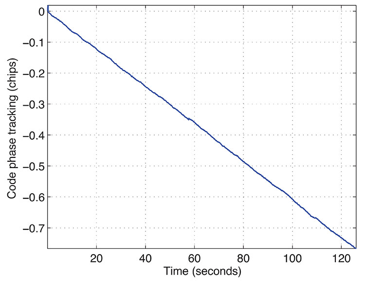
    FIGURE 3 shows the code-phase measurement made by GEMS. Although the scenario was static in terms of propagation delay, the code-phase measurement linearly decreases over time. This is because the Navys and GEMS clocks are independent and are drifting with respect to each other.

    FIGURE 3. GEMS code-phase measurements on GPS L1 C/A signal, EWFA dynamic scenario.
    FIGURE 3. GEMS code-phase measurements on GPS L1 C/A signal, EWFA dynamic scenario.

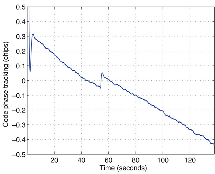
    The second observation is that the introduction of the EWFA induced, as expected, a bias in the measurement. If one removes the clock drifts, the bias is estimated to be 0.085 chips (approximately 25 meters). According to theory, an EWFA induces a bias equal to half the lead or lag value. A value of 171 nanoseconds is equivalent to about 50 meters.

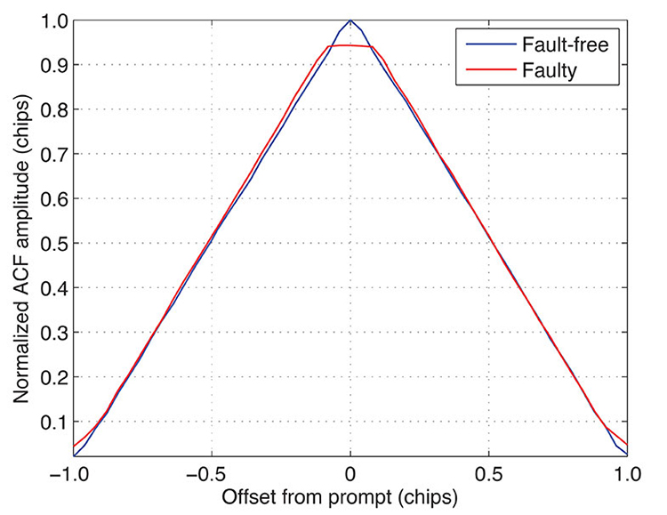
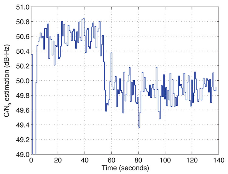
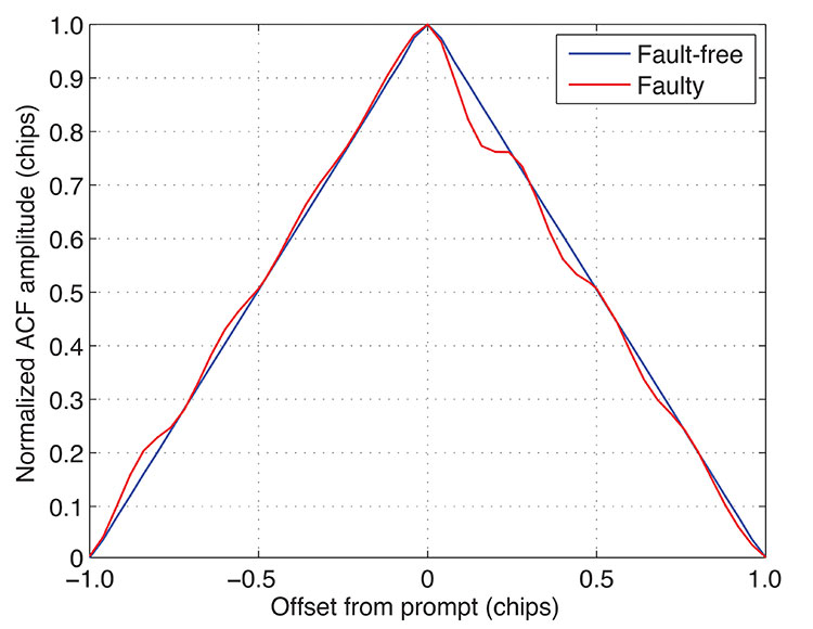
    FIGURE 4 represents the ACFs computed by GEMS during the scenario. It appears that when the EWFA is enabled, the autocorrelation function is flattened at its top, which is typical of EWFA distortions. Eventually, FIGURE 5 showed that the EWFA also results in a decrease of the measured C/N0, which is completely coherent with the flattened correlation function obtained when EWFA is on.

    FIGURE 4. GEMS ACF computation on GPS L1 C/A signal, EWFA dynamic scenario.
    FIGURE 4. GEMS ACF computation on GPS L1 C/A signal, EWFA dynamic scenario.
    FIGURE 5. GEMS C/N0 measurement on GPS L1 C/A signal, EWFA dynamic scenario.
    FIGURE 5. GEMS C/N0 measurement on GPS L1 C/A signal, EWFA dynamic scenario.

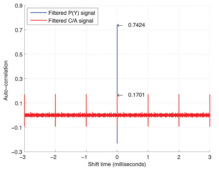
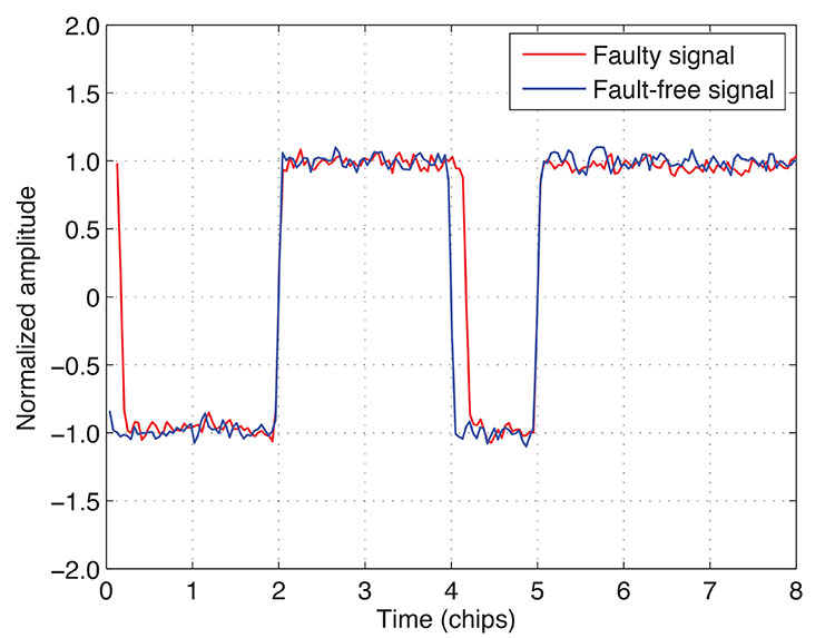
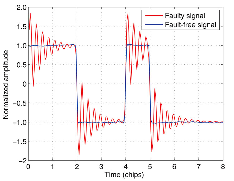
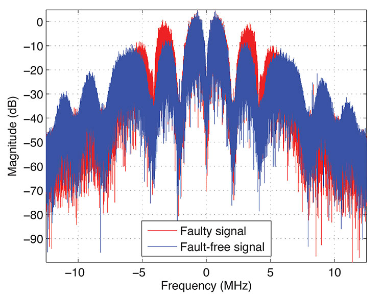
    Additional analysis has been conducted with Matlab to confirm Navys’ capacity. A GPS signal acquisition and tracking routine was modified to perform coherent accumulation of GPS signals. This operation is meant to extract the signal out of the noise, and to enable observation of the code chips. After Doppler and code-phase estimation, the signal is post-processed and 1,000 signal periods are accumulated. The result, shown in FIGURE 6, confronts fault-free (blue) and EWFA-affected (red) code chips. Again, the lag of 171 nanoseconds is clearly observed. The analysis concludes with FIGURE 7, which shows the fault-free (blue) and the faulty (red) signal spectra. Again, the presence of spikes in the faulty spectrum is characteristic of EWFA.

    FIGURE 6. Fault-free vs. EWFA GPS L1 C/A signal.
    FIGURE 6. Fault-free vs. EWFA GPS L1 C/A signal.
    FIGURE 7. Fault-free vs. EWFA GPS L1 C/A signal power spectrum density.
    FIGURE 7. Fault-free vs. EWFA GPS L1 C/A signal power spectrum density.

    EWFB, static scenario. The same experiments as for EWFA were conducted for EWFB. Fault-free and faulty (EWFB with a resonance frequency of 8 MHz and a damping factor of 7 MHz) signals were simultaneously generated and observed using an oscilloscope and a spectrum analyzer. The baseband temporal signal undergoes the same default as that of the EWFA because of the Navys high-pass filter. However, the oscillations induced by the EWFB are clearly observed.

    The spectrum distortion induced by the EWFB at the L1 frequency is amplified around 8 MHz, which is consistent with the applied failure.

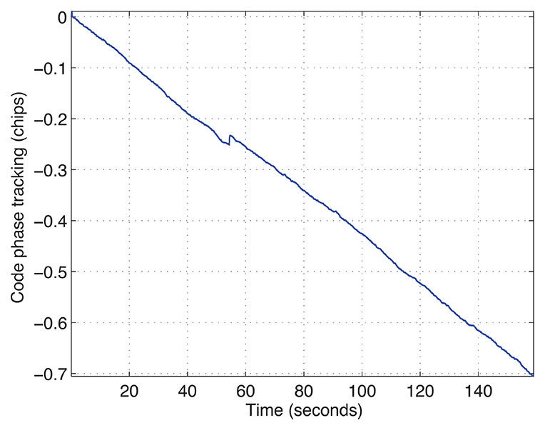
    EWFB, dynamic scenario. Navys was then configured to generate one fault-free GPS L1 C/A signal at RF. The RF output was plugged into the GEMS RF front end, and acquisition was launched. One minute later, an EWFB distortion with a resonance frequency of 4 MHz and a damping factor of 2 MHz was applied. As for the EWFA experiments, the GEMS measurements were analyzed to verify the correct application of the failure. The code-phase measurements, illustrated in FIGURE 8, show again that the Navys and GEMS clocks are drifting with respect to each other. Moreover, it is clear that the application of the EWFB induced a bias of about 5.2 meters on the code-phase measurement. One should notice that this bias depends upon the chip spacing used for tracking. Matlab simulations were run considering the same chip spacing as for GEMS, and similar tracking biases were observed.

    FIGURE 8. GEMS code-phase measurements on GPS L1 C/A signal, EWFB dynamic scenario.
    FIGURE 8. GEMS code-phase measurements on GPS L1 C/A signal, EWFB dynamic scenario.

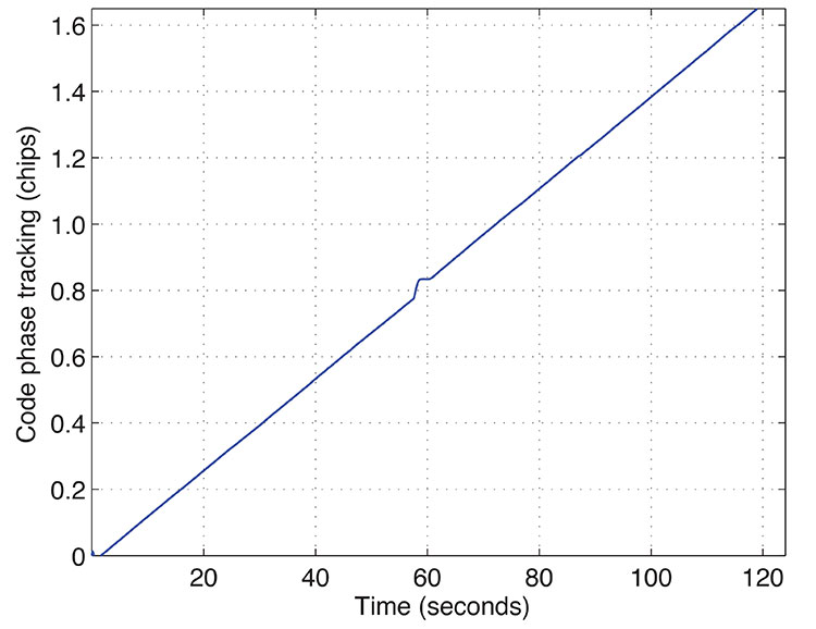
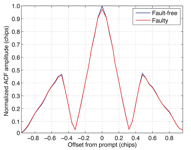
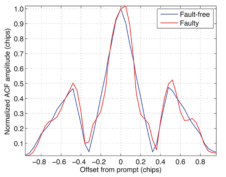
    FIGURE 9 shows the ACF produced by GEMS. During the first minute, the ACF looks like a filtered L1 C/A correlation function. Afterward, undulations distort the correlation peak.

    FIGURE 9. GEMS ACF computation on GPS L1 C/A signal, EWFB dynamic scenario.
    FIGURE 9. GEMS ACF computation on GPS L1 C/A signal, EWFB dynamic scenario.

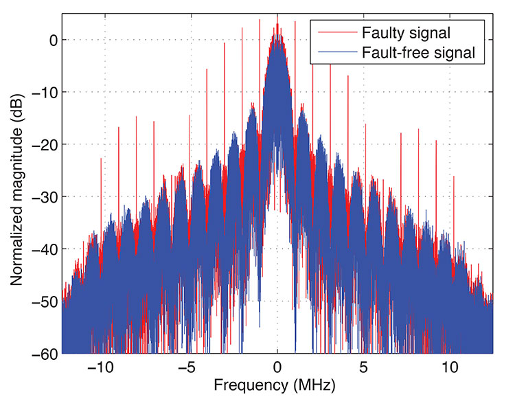
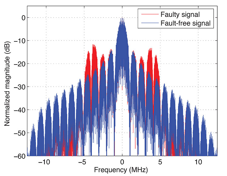
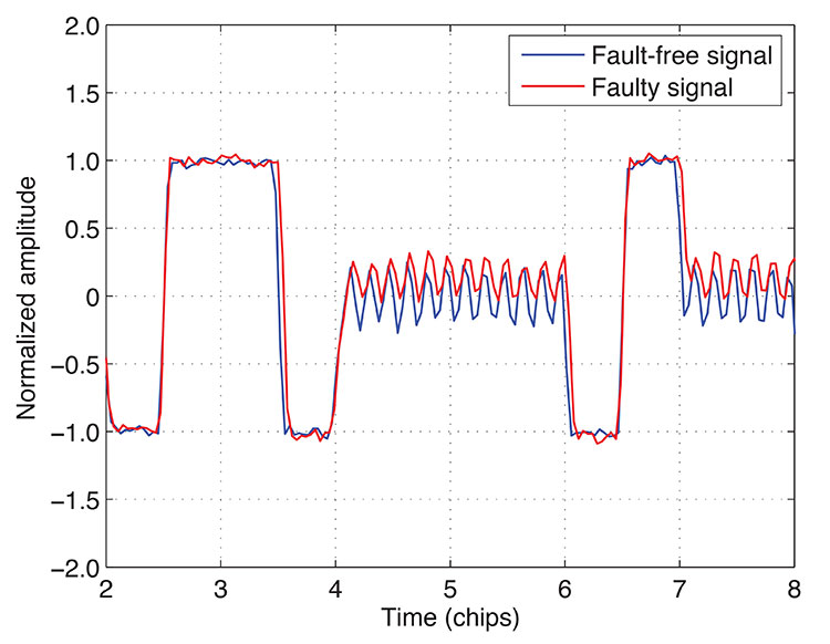
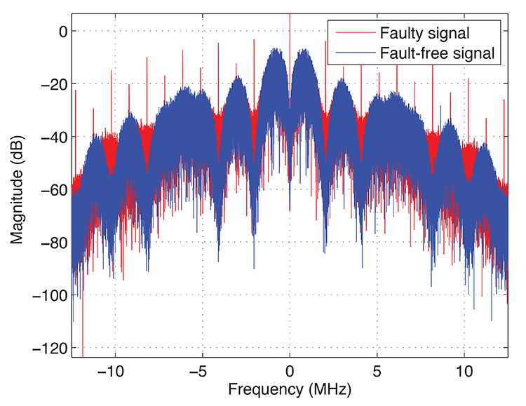
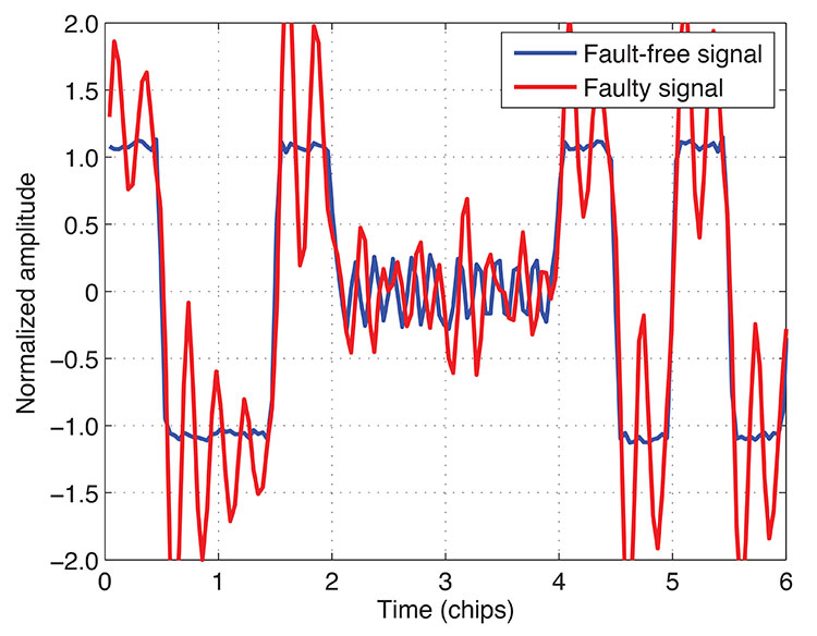
    Again, additional analysis has been conducted with Matlab, using a GPS signal acquisition and tracking routine. A 40-second accumulation enabled comparison of the faulty and fault-free code chips. FIGURE 10 shows that the faulty code chips are affected by undulations with a period of 244 nanoseconds, which is consistent with the 4 MHz resonance frequency. This temporal signal was then used to compute the spectrum, as shown in FIGURE 11. The figure shows well that the faulty L1 C/A spectrum (red) secondary lobes are raised up around the EWFB resonance frequency, compared to the fault-free L1 C/A spectrum (blue).

    FIGURE 10. Fault-free vs EWFB GPS L1 C/A signal.
    FIGURE 10. Fault-free vs EWFB GPS L1 C/A signal.


    FIGURE 11. Fault-free vs EWFB GPS L1 C/A signal power spectrum density.
    FIGURE 11. Fault-free vs EWFB GPS L1 C/A signal power spectrum density.

    Galileo E1 CBOC(6, 1, 1/11). In the second part of the experiments, Navys was configured to generate the Galileo E1 Open Service (OS) signal instead of the GPS L1 C/A signal. The goal was to assess the impact of EWs on such a modernized signal.

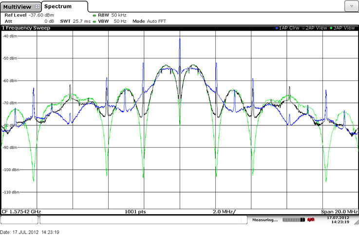
    EWFA, static scenario. First, the same Galileo E1 BC signal was generated using two different Navys channels. One was affected by EWFA, and the other was not. The spectra of the obtained signals were observed using a spectrum analyzer. The spectrum of the signal produced by the fault-free channel shows the BOC(1,1) main lobes, around 1 MHz, and the weaker BOC(6,1) main lobes, around 6 MHz. The power spectrum of the signal produced by the EWFA channel has a lag of 5 samples at 120 times f0 (40 nanoseconds). Again, spikes appear at intervals of f0, which is consistent with theory. The signal produced by the same channel, but with a lag set to 21 samples (171.07 nanoseconds) was also seen. Such a lag should not be experienced on CBOC(6,1,1/11) signals as this lag is longer than the BOC(6,1) subcarrier half period (81 nanoseconds). This explains the fact that the BOC(6,1) lobes do not appear anymore in the spectrum.

    EWFB, static scenario. The same experiments as for EWFA were conducted for EWFB. Fault-free and faulty (EWFB with a resonance frequency of 8 MHz and a damping factor of 7 MHz) signals were simultaneously generated and observed using the spectrum analyzer. The spectrum distortion induced by the EWFB at the E1 frequency was evident. The spectrum is amplified around 8 MHz, which is consistent with the applied failure.

    EWFA, dynamic scenario. The same scenario as for the GPS L1 C/A signal was run with the Galileo E1 signal: first, for a period of one minute, a fault-free signal was generated, followed by a period of one minute with the faulty signal. GEMS was switched on and acquired and tracked the two-minute-long signal. Its code-phase measurements, shown in FIGURE 12, reveal a tracking bias of 6.2 meters. This is consistent with theory, where the set lag is equal to 40 nanoseconds (12.0 meters). GEMS-produced ACFs show the distortion of the correlation function in FIGURE 13. The distortion is hard to observe because the applied lag is small.

    FIGURE 12. GEMS code-phase measurements on Galileo E1 pilot signal, EWFA dynamic scenario.
    FIGURE 12. GEMS code-phase measurements on Galileo E1 pilot signal, EWFA dynamic scenario.
    FIGURE 13. GEMS ACF computation on Galileo E1 pilot signal, EWFA dynamic scenario.
    FIGURE 13. GEMS ACF computation on Galileo E1 pilot signal, EWFA dynamic scenario.

    A modified version of the GPS signal acquisition and tracking Matlab routine was used to acquire and track the Galileo signal. It was configured to accumulate 50 seconds of fault-free signal and 50 seconds of a faulty signal. This operation enables seeing the signal in the time domain, as in FIGURE 14. Accordingly, the following observations can be made:

    • The E1 BC CBOC(6,1,1/11) signal is easily recognized from the blue curve (fault-free signal).
    • The EWFA effect is also seen on the BOC(1,1) and BOC(6,1) parts. The observed lag is consistent with the scenario (five samples at 120 times f0 ≈ 0.04 chips).
    • The lower part of the BOC(6,1) seems absent from the red signal. Indeed, the application of the distortion divided the duration of these lower parts by a factor of two, and so multiplied their Fourier representation by two. Therefore, the corresponding main lobes should be located around 12 MHz. At the receiver level, the digitization is being performed at 25 MHz; this signal is close to the Shannon frequency and is therefore filtered by the anti-aliasing filter.
    FIGURE 14. Fault-free vs EWFA Galileo E1 signal.
    FIGURE 14. Fault-free vs EWFA Galileo E1 signal.

    The power spectrum densities of the obtained signals were then computed. FIGURE 15 shows the CBOC(6,1,1/11) fault-free signal in blue and the faulty CBOC(6,1,1/11) signal, with the expected spikes separated by 1.023 MHz.

    FIGURE 15. Fault-free vs. EWFA Galileo E1 signal power spectrum density.
    FIGURE 15. Fault-free vs. EWFA Galileo E1 signal power spectrum density.

    It is noteworthy that the EWFA has been applied to the entire E1 OS signal, which is B (data component) minus C (pilot component). EWFA could also affect exclusively the data or the pilot channel. Although such an experiment was not conducted during our research, Navys is capable of generating EWFA on the data component, the pilot component, or both.

    EWFB, dynamic scenario. In this scenario, after one minute of a fault-free signal, an EWFB, with a resonance frequency of 4 MHz and a damping factor of 2 MHz, was activated. The GEMS code-phase measurements presented in FIGURE 16 show that the EWFB induces a tracking bias of 2.8 meters. As for GPS L1 C/A signals, it is to be noticed that the bias induced by EWFB depends upon the receiver characteristics and more particularly the chip spacing used for tracking.

    FIGURE 16. GEMS code-phase measurements on Galileo E1 pilot signal, EWFB dynamic scenario.
    FIGURE 16. GEMS code-phase measurements on Galileo E1 pilot signal, EWFB dynamic scenario.

    The GEMS produced ACFs are represented in FIGURE 17. After one minute, the characteristic EWFB undulations appear on the ACF.

    FIGURE 17. GEMS ACF computation on Galileo E1 pilot signal, EWFB dynamic scenario.
    FIGURE 17. GEMS ACF computation on Galileo E1 pilot signal, EWFB dynamic scenario.

    In this case, signal accumulation was also performed to observe the impact of EWFB on Galileo E1 BC signals. The corresponding representation in the time domain is provided in FIGURE 18, while the Fourier domain representation is provided in FIGURE 19. From both points of view, the application of EWFB is compliant with theoretical models. The undulations observed on the signal are coherent with the resonance frequency (0.25 MHz ≈ 0.25 chips), and the spectrum also shows the undulations (the red spectrum is raised up around 4 MHz).

    FIGURE 18. Fault-free vs EWFB Galileo E1 signal.
    FIGURE 18. Fault-free vs EWFB Galileo E1 signal.
    FIGURE 19. Fault-free vs. EWFB Galileo E1 signal power spectrum density.
    FIGURE 19. Fault-free vs. EWFB Galileo E1 signal power spectrum density.

    Conclusion

    Navys is a multi-constellation GNSS simulator, which allows the generation of all modeled EWF (types A and B) on both GPS and Galileo signals. Indeed, the Navys design makes the EWF application independent of the signal modulation and carrier frequency.

    The International Civil Aviation Organization model has been adapted to Galileo signals, and the correct application of the failure modes has been verified through RF simulations. The theoretical effects of EWF types A and B on waveforms, spectra, autocorrelation functions and code-phase measurements have been confirmed through these simulations.

    For a given lag value, the tracking biases induced by type A EWF distortions are equal on GPS and Galileo signals, which is consistent with theory.

    Eventually, for a given resonance frequency-damping factor combination, the type B EWF distortions induce a tracking bias of about 5.2 meters on GPS L1 C/A measurements and only 2.8 meters on Galileo E1 C measurements. This is mainly due to the fact that the correlator tracking spacing was reduced for Galileo signal tracking (± 0.15 chips instead of ± 0.5 chips). (Additional figures showing oscilloscope and spectrum analyzer screenshots of experimental results are available in the online version of this article.)

    Acknowledgments

    This article is based on the paper “Generating Evil WaveForms on Galileo Signals using NAVYS” presented at the 6th ESA Workshop on Satellite Navigation Technologies and the European Workshop on GNSS Signals and Signal Processing, Navitec 2012, held in Noordwijk, The Netherlands, December 5–7, 2012.

    Manufacturers

    In addition to the Navys simulator, the experiments used a Saphyrion sagl GDAS-1 GNSS data acquisition system, a Rohde & Schwarz GmbH & Co. KG RTO1004 digital oscilloscope, and a Rohde & Schwarz FSW26 signal and spectrum analyzer.


    MATHIEU RAIMONDI is currently a GNSS systems engineer at Thales Alenia Space France (TAS-F). He received a Ph.D. in signal processing from the University of Toulouse (France) in 2008.

    ERIC SENANT is a senior navigation engineer at TAS-F. He graduated from the Ecole Nationale d’Aviation Civile (ENAC), Toulouse, in 1997.

    CHARLES FERNET is the technical manager of GNSS system studies in the transmission, payload and receiver group of the navigation engineering department of the TAS-F navigation business unit. He graduated from ENAC in 2000.

    RAPHAEL PONS is currently a GNSS systems engineering consultant at Thales Services in France. He graduated as an electronics engineer in 2012 from ENAC.

    HANAA AL BITAR is currently a GNSS systems engineer at TAS-F. She graduated as a telecommunications and networks engineer from the Lebanese Engineering School of Beirut in 2002 and received her Ph.D. in radionavigation in 2007 from ENAC, in the field of GNSS receivers.

    FRANCISCO AMARILLO FERNANDEZ received his Master’s degree in telecommunication engineering from the Polytechnic University of Madrid. In 2001, he joined the European Space Agency’s technical directorate, and since then he has worked for the Galileo program and leads numerous research activities in the field of GNSS evolution.

    MARC WEYER is currently working as the product manager in ELTA, Toulouse, for the GNSS simulator and recorder.


    Additional Images

    GEMS graphical interface.
    GEMS graphical interface.
    Observation of EWF type A on GPS L1 C/A signal with an oscilloscope.
    Observation of EWF type A on GPS L1 C/A signal with an oscilloscope.
    Impact of EWF A on GPS L1 C/A signal spectrum for 0 (green), 41 (black), and 171 (blue) nanosecond lag.
    Impact of EWF A on GPS L1 C/A signal spectrum for 0 (green), 41 (black), and 171 (blue) nanosecond lag.
    Observation of EWF type A on GPS L1 C/A signal with an oscilloscope.
    Observation of EWF type A on GPS L1 C/A signal with an oscilloscope.
    Impact of EWF B on GPS L1 C/A signal spectrum for Fd = 8 MHz and σ = 7 MHz.
    Impact of EWF B on GPS L1 C/A signal spectrum for fd = 8 MHz and σ = 7 MHz.
    Impact of EWF A on Galileo E1 BC signal spectrum for 0 (green), 40 (black), and 171 (blue) nanosecond lag.
    Impact of EWF A on Galileo E1 BC signal spectrum for 0 (green), 40 (black), and 171 (blue) nanosecond lag.
    Navys hardware equipment – Blackline edition.
    Navys hardware equipment – Blackline edition.

    Further Reading

    • Authors’ Conference Paper

    “Generating Evil WaveForms on Galileo Signals using NAVYS” by M. Raimondi, E. Sénant, C. Fernet, R. Pons, and H. AlBitar in Proceedings of Navitec 2012, the 6th ESA Workshop on Satellite Navigation Technologies and the European Workshop on GNSS Signals and Signal Processing, Noordwijk, The Netherlands, December 5–7, 2012, 8 pp., doi: 10.1109/NAVITEC.2012.6423071.

    • Threat Models

    “A Novel Evil Waveforms Threat Model for New Generation GNSS Signals: Theoretical Analysis and Performance” by D. Fontanella, M. Paonni, and B. Eissfeller in Proceedings of Navitec 2010, the 5th ESA Workshop on Satellite Navigation Technologies, Noordwijk, The Netherlands, December 8–10, 2010, 8 pp., doi: 10.1109/NAVITEC.2010.5708037.

    “Estimation of ICAO Threat Model Parameters For Operational GPS Satellites” by A.M. Mitelman, D.M. Akos, S.P. Pullen, and P.K. Enge in Proceedings of ION GPS 2002, the 15th International Technical Meeting of the Satellite Division of The Institute of Navigation, Portland, Oregon, September 24–27, 2002, pp. 12–19.

    • GNSS Signal Deformations

    “Effects of Signal Deformations on Modernized GNSS Signals” by R.E. Phelts and D.M. Akos in Journal of Global Positioning Systems, Vol. 5, No. 1–2, 2006, 9 pp.

    “Robust Signal Quality Monitoring and Detection of Evil Waveforms” by R.E. Phelts, D.M. Akos, and P. Enge in Proceedings of ION GPS-2000, the 13th International Technical Meeting of the Satellite Division of The Institute of Navigation, Salt Lake City, Utah, September 19–22, 2000, pp. 1180–1190.

    “A Co-operative Anomaly Resolution on PRN-19” by C. Edgar, F. Czopek, and B. Barker in Proceedings of ION GPS-99, the 12th International Technical Meeting of the Satellite Division of The Institute of Navigation, Nashville, Tennessee, September 14–17, 1999, pp. 2269–2271.

    • GPS Satellite Anomalies and Civil Signal Monitoring

    An Overview of Civil GPS Monitoring by J.W. Lavrakas, a presentation to the Southern California Section of The Institute of Navigation at The Aerospace Corporation, El Segundo, California, March 31, 2005.

    • Navys Signal Simulator

    “A New GNSS Multi Constellation Simulator: NAVYS” by G. Artaud, A. de Latour, J. Dantepal, L. Ries, N. Maury, J.-C. Denis, E. Senant, and T. Bany in  Proceedings of ION GPS 2010, the 23rd International Technical Meeting of the Satellite Division of The Institute of Navigation, Portland, Oregon, September 21–24, 2010, pp. 845–857.

    “Design, Architecture and Validation of a New GNSS Multi Constellation Simulator : NAVYS” by G. Artaud, A. de Latour, J. Dantepal, L. Ries, J.-L. Issler, J. Tournay, O. Fudulea, J.-M. Aymes, N. Maury, J.-P. Julien , V. Dominguez, E. Senant, and M. Raimondi in  Proceedings of ION GPS 2009, the 22nd International Technical Meeting of the Satellite Division of The Institute of Navigation, Savannah, Georgia, September 22–25, 2009, pp. 2934–2941.

  • Innovation: Interfacing Clearly

    Innovation: Interfacing Clearly

    A New Approach to the Design and Development of Global Navigation Satellite Systems

    By Daniele Gianni, Marco Lisi, Pierluigi De Simone, Andrea D’Ambrogio, and Michele Luglio

    GPS World photo
    INNOVATION INSIGHTS by Richard Langley

    MY FIRST DEGREE is in applied physics from the University of Waterloo. Founded in 1957, Waterloo was one of the first universities to introduce co-operative education. Co-operative education (or “co-op” as it is commonly known) is a program that uses both classroom study and temporary jobs to provide students with practical experience. Applied Physics was a co-op program and I worked in both industry and research environments including stints at Philips Electronics and the Atomic Energy of Canada Limited’s Chalk River Laboratories.

    Both on campus and on the job, I met fellow co-op students from a variety of disciplines including mathematics (computer science) and various branches of engineering. One of those was systems design engineering or systems engineering for short. At that time, I really didn’t know much about systems engineering except that it was an all-encompassing branch of engineering and the most challenging of all of the engineering programs at Waterloo — at least according to the students in the program.

    Systems engineering is an interdisciplinary field of engineering focusing on the design and management of complex engineering projects. According to the International Council on Systems Engineering, systems engineers establish processes “to ensure that the customer and stakeholder’s needs are satisfied in a high quality, trustworthy, cost efficient and schedule compliant manner throughout a system’s entire life cycle. This process is usually comprised of the following seven tasks: State the problem, Investigate alternatives, Model the system, Integrate, Launch the system, Assess performance, and Re-evaluate [or, SIMILAR, for short].”

    Central to the systems engineering process and the end-product design is the generation of models. Many types of system models are used, including physical analogs, analytical equations, state machines, block diagrams, functional flow diagrams, object-oriented models, computer simulations, and even mental models. (If you want to learn a bit about mental and other kinds of models, including how to fix radios by thinking, you could do no better than to look at some of Richard Feynman’s writings including the eminently readable “Surely You’re Joking, Mr. Feynman!”: Adventures of a Curious Character.)

    As aids to the modeling process, systems engineers have developed specialized modeling languages including the Unified Modeling Language (UML) and the Systems Modeling Language (SysML). These are graphical-based languages that can be used to express information or knowledge about systems in a structure that is defined by a consistent set of rules. Both UML and SysML are widely used in systems engineering. However, both are limited when it comes to representing the signal-in-space (SIS) interfaces for global navigation satellite systems.

    In this month’s column, a team of authors affiliated with the Galileo project discusses the Interface Communication Modeling Language, an extension of UML that allows engineers to clearly represent SIS interfaces, critical for the design of GNSS receivers.


    “Innovation” is a regular feature that discusses advances in GPS technology andits applications as well as the fundamentals of GPS positioning. The column is coordinated by Richard Langley of the Department of Geodesy and Geomatics Engineering, University of New Brunswick. He welcomes comments and topic ideas. To contact him, see the “Contributing Editors” section on page 4.


    In this article, we present the results of ongoing research on the use of a modeling language, namely Interface Communication Modeling Language (ICML), for signal-in-space (SIS) interface specification of global navigation satellite systems (GNSS). Specifications based on modeling languages (also known as model-based specifications) have proven to offer a wide range of benefits to systems engineering activities, for supporting system interoperability, reducing design risk, automating software development, and so on. We argue that similar benefits can be obtained for satellite navigation systems and receivers, if a model-based approach is used for defining and expressing the SIS interface specification. In particular, we outline how a model-based SIS interface specification can support the identification of solutions to two key issues: GNSS interoperability and the design of GNSS receivers, particularly Galileo receivers. Both issues are becoming increasingly central to the Galileo program since it entered the In-Orbit-Validation (IOV) phase and is steadily approaching the 2014 milestone, when the first early services — the Open Service (OS) and the Search and Rescue Service — will be provided to users.

    GNSS interoperability concerns the integration of different GNSS with the purpose of being used together, along with regional positioning systems, to provide a seamless navigation capability and improved services in terms of availability, continuity, accuracy, and integrity, for example. GNSS interoperability should be addressed in terms of intra-GNSS interoperability and GNSS-receiver interoperability. The intra-GNSS interoperability concerns the data exchanged among the GNSS, including coordination to guarantee data coherence and consistency over time. For example, GNSS may need to share terrestrial reference frames and constantly synchronize their global time references. On the other hand, GNSS-receiver interoperability concerns the capability of the receiver to use independent GNSS signals for the computation of positions globally. This capability implicitly requires that the receiver computations are decoupled from the SIS interface of any particular GNSS. A key condition to achieve this decoupling is that the SIS interface specification is available in a consistent, unambiguous, and possibly standard format, which can support engineers to more effectively design interoperable receivers. A model-based SIS interface specification would considerably facilitate this as it enables designers to use the processing capabilities of a computer system for the verification of the specification consistency and completeness, for example. Moreover, a model-based SIS interface specification would ease the visual and electronic inspection of the data messages, therefore facilitating the automatic identification of different data representations for the same orbital and temporal parameters.

    The design of GNSS receivers, and particularly those for Galileo, is increasingly of interest, and a model-based SIS interface specification can similarly support the definition of future solutions. For Galileo, specifically, the receiver design is critical to support the marketing strategies that are promoting the use of Galileo services. Key issues underlying any marketing strategy concern the Galileo receiver market appealing from a cost-to-performance ratio point of view. As Galileo receivers may require new design and adaptation of existing software (SW) or hardware (HW), as well as new production chains, higher costs — in particular non-recurring ones — are likely to occur for the production of the Galileo receivers with respect to the well-established GPS receivers. As a consequence, limitations may be experienced in market penetration and in the growth velocity of Galileo receivers’ share of the receiver market. In turn, this may hinder the estimated economic return for the Galileo project.

    Preventing and counteracting this possibility is therefore a critical issue if we aim to achieve the widest possible success of the Galileo project. Market barriers inherently originate from the following needs:

    • Designing new SW and HW solutions for Galileo receivers;
    • Reusing existing SW and HW for GPS receivers;
    • Converting existing production chains to the new Galileo-specific SW and HW solutions.

    GNSS receivers often use established mathematical models that can determine the receiver position from a fundamental set of parameters, such as satellite orbit and system time. As a consequence, the intrinsic representation of the parameter set is a major factor in the adaptation of the existing design and implementation of SW and HW solutions.

    To reduce the impact of the above needs, a model-based SIS interface specification may play a pivotal role in several ways, such as:

    • reducing ambiguities in the Galileo SIS interface specification;
    • enhancing the communication with the involved stakeholders;
    • linking the SIS interface specification to the design schemas of GNSS receivers — particularly Galileo ones — for tracing the interface elements onto the receiver functional and physical schema, thereby supporting the reuse and adaptation of existing HW and SW solutions;
    • supporting the model-based design of security solutions for blocking, jamming, and spoofing.

    Galileo Project

    In October 2012, the final two IOV satellites were launched into orbit, completing the designed configuration for the Galileo IOV phase — the initial stage of the Galileo constellation development. In this phase, preliminary validation tests will be performed and the initial navigation message will be broadcast to the Galileo ground segment for further validation. Shortly after the conclusion of this phase, a series of launches will take place to gradually deploy the remaining 26 satellites that will form the Galileo Full Operational Capability (FOC) configuration. Currently, the Galileo Early Open Service (EOS) is expected to be available by the end of 2014. The EOS will provide ranging capabilities and will enable receiver manufacturers to begin to design and test their technological solutions for Galileo receivers and Galileo overlay services, such as search and rescue.

    In the meantime, the European GNSS Agency has been established and assigned the governance of the Galileo sub-systems, including activities such as:

    • initiating and monitoring the implementation of security procedures and performing system security audits;
    • system infrastructure management, maintenance, improvement, certification, and standardization, and service provision;
    • development and deployment of activities for the evolution and future generations of the systems, including procurement activities;
    • contributing to the exploitation of the systems, including the marketing and promotion of applications and services, including market analysis.

    With the now-rapid development of the Galileo project, it becomes increasingly important to support the receiver manufacturers in the design and implementation of global navigation solutions based on the Galileo services. This is necessary to guarantee the widespread use of the Galileo services, particularly in an increasingly crowded GNSS panorama.

    Model-Based Systems Engineering

    Model-based systems engineering (MBSE) is predicated on the notion that a system is developed by use of a set of system models that evolve throughout the development lifecycle, from abstract models at the early stages down to the operational system. A visual presentation is provided by FIGURE 1, which shows the roles of MBSE approaches within the systems engineering V-shaped process. Specifically, the MBSE approaches enable the designer to effectively trace the requirements and design alternatives on the descending branch of the “V.” For the same characteristics, MBSE facilitates the verification through a model repository that interconnects not only the design products, but also the stakeholders involved in the entire process. In addition, MBSE approaches support the automatic generation of the documentation and of other artifacts, particularly software. All of these capabilities eventually enable the validation of the implementation activities on the ascending branch of the V-process. Also, in this case, MBSE and the model repository play a major role in connecting design to implementation, and users and designers to developers.

    FIGURE 1. Systems engineering V-process supported by an model-based systems engineering with model repository (courtesy of the INCOSE Survey).
    FIGURE 1. Systems engineering V-process supported by an model-based systems engineering with model repository (courtesy of the INCOSE Survey).

    Main Concepts. MBSE approaches are gaining increasing popularity with the widespread adoption of standard modeling languages, such as Unified Modeling Language (UML) and Systems Modeling Language (SysML).

    UML is a formally defined general-purpose graphical language and is mainly used in the context of software systems development. It has been developed and is being managed by the Object Management Group and is the core standard of the Model Driven Architecture (MDA) effort, which provides a set of standards to shift from code-centric to model-driven software development. By use of an MDA-based approach, a software system is built by specifying and executing a set of automated model transformations.

    SysML is defined as an extension of UML and provides a general-purpose modeling language for systems engineering applications (See FIGURE 2). SysML supports MBSE approaches in the development of complex systems that include hardware, software, information, processes, personnel, and facilities.

    FIGURE 2. UML-SysML relationships. (UML 2 is the second generation version of UML introduced in 2005.)
    FIGURE 2. UML-SysML relationships. (UML 2 is the second generation version of UML introduced in 2005.)

    Advantages. With respect to the conventional document-based approaches, MBSE approaches present the following advantages:

    • Conformance to standard specifications and availability of development tools;
    • Increased level of automation due to the formal specification and execution of model transformations that take as input a model at a given level of abstraction and yield as output a refined model at a lower level of abstraction;
    • Better understanding of the system in its operational context;
    • Support for simulation activities at different levels of detail and at different development stages, from concept exploration to dynamic system optimization;
    • Support for the coherent extension of standard modeling languages to adapt them to a specific target or domain.

    These capabilities have motivated and have been sustaining an increasing trend of moving from document-centric to model-centric systems engineering.

    ICML Language

    UML and SysML are widely used languages for MBSE. A plethora of tools and technologies are available to compose models, transform models into documents, derive software products from models, and share and reuse models by means of repositories. However, neither of these languages offers capabilities for the representation of SIS interfaces, which are the critical interfaces for the design of Galileo receivers. For this reason, we have introduced ICML: a modeling language that can enable a full MBSE approach for the design of Galileo receivers. Moreover, ICML extends UML, and therefore it can integrate with system specifications based on compliant technologies as well as be used within standard tools.

    Layout of Interface Specification. The typical layout of ICML-based interface specification is shown in FIGURE 3. The specification covers the definition of both the message structure and conversion processes. The message structure consists of five abstraction levels, and describes how the data is structured within the message. The conversion processes describe how the data values are transformed between adjacent levels of the message specification.

    FIGURE 3. Layout of ICML-based interface specifications.
    FIGURE 3. Layout of ICML-based interface specifications.

    The message structure is defined at five levels: Data Definition, (Logical) Binary Coding, Logical Binary Structure, Physical Binary Coding, and Physical Signal, each covering specific aspects of the SIS interface specification.

    For example, the Data Definition level covers the specification of the logical data structure, which includes the data items composing the message information. A data item is either of application or control type. An application data item represents a domain-specific concept that conveys the information expected by the message recipient. On the other hand, a control data item represents a domain-independent concept that can support the correctness and integrity verification of the associated application data items. A data item can also be associated with semantic and pragmatic definitions. The former specifies the meaning of the data item and the latter specifies the contextual interpretation for the semantic definition.

    Analogously, the Binary Coding level covers the specification of the binary coding for each of the data items defined at the above level. For a data item, the binary coding is represented as a binary sequence and it includes at least a sequence identifier, the semantic definition, and the pragmatic definitions. Similarly to the above level, the semantic and pragmatic definitions enrich the interface specification, conveying an accurate representation of the binary coding.

    The conversion processes describe the activities to be performed for deriving message values between adjacent levels of the above structural specification. As shown in Figure 3, eight processes should be defined to specify all the conversions between adjacent levels. For example, the DataDefinition2BinaryCoding process defines the activities to be performed for the derivation of the logical binary sequences representing data values. Similarly, the LogicalBinary2PhysicalBinary process defines the activities for the implementation of convolution or encryption algorithms on the logical binary sequence. However, these processes do not always need to be explicitly defined. In particular, if the implementation of a process is trivial or standard, a textual note referring to an external document may suffice for the specification purposes.

    The first prototypal version of ICML has been implemented and can be used within the open source TopCased tool. The prototypal version is available under the GNU General Public License (GPL) v3.0 from the ICML project website. We applied the profile and developed the example ICML-based specification given below.

    Galileo-Like Specification. An ICML-based specification of a Galileo-like OS interface, concerning only the above-defined level 3, would display as shown in FIGURE 4. This figure specifically details a part of a reduced F/NAV (the freely accessible navigation message provided by the E5a signal for the Galileo OS) structure consisting of one data frame made up of two F/NAV subframes.

    FIGURE 4. Example of ICML-based specification of an F/NAV-like message structure at the Logical Binary Coding level.
    FIGURE 4. Example of ICML-based specification of an F/NAV-like message structure at the Logical Binary Coding level.

    Benefits. ICML can bring the above-mentioned MBSE benefits to support GNSS interoperability and to GNSS and Galileo receiver design. For example, ICML can:

    • provide a reference guideline for structuring the specification data and thus facilitating the communication between the Galileo SIS designers and the receiver producers;
    • ease visual inspection of the specification for verification purposes and for the identification of data incompatibilities of two GNSS systems;
    • convey the data semantics as well as the measurement units, to guarantee that the binary data from different GNSS are correctly decoded and interpreted;
    • support syntactical model validation using existing tools;
    • provide support for future advance exploitation by means of a machine-readable data format.

    In particular, the availability of a machine-readable format is also the basis for advanced use cases that can exploit the capabilities of modern computer technologies.

    Advanced Future Use Cases. In line with the above-mentioned MBSE model exploitations, we foresee a number of possible exploitation cases:

    • Automatic generation of the interface specification documents;
    • Collaborative development of the interface specification;
    • Automatic completeness and consistency checking of the interface specification;
    • Integration of SIS specifications with model-driven simulation engineering approaches for the simulation of single- and multi-GNSS receivers;
    • Integration of SIS specifications with receiver design models in SysML, for requirements traceability and reuse of existing GNSS solutions.

    The automatic generation of interface specification documents can be an important capability during the lifecycle of a specification. For example, the specification may be updated several times during the interface design, and the textual documentation may need to be produced several times. Using a model-based approach, it is possible to automate the error-prone activities related to the document writing as well as other important functions such as specification versioning.

    Complex system specifications are often the product of collaborating teams, which may occasionally be geographically dispersed. Using a model-based approach, the interface specification can be stored within a version control system that can be concurrently accessed by team members.

    Completeness and consistency checking is also a manual activity, which demands a high degree of mental attention, and it is consequently highly error prone. Once the specification is available in a machine-readable format, the checking can be easily automated by specifying the verification rules that the interface model must satisfy.

    Existing technologies support the simulation of single- and multi-GNSS receivers. As the SIS specification has a major impact on the internal structure of the receiver, the interface specification is a key input for developing GNSS simulators as well as for determining the boundary properties of the input signal into the receiver, including the admitted analog signal and the format of the digital data.

    Moreover, the model-based interface specification can be integrated with a receiver design schema in SysML. This would be important to provide traceability between the interface requirements and the receiver’s functional and physical components. In the following section, we provide an outline for a preliminary integration between the interface specification and the receiver design.

    Designing Galileo Receivers

    Model-based interface specifications can support the design of Galileo receivers in several ways. For example, a specification can provide a link between Galileo requirements down to the Galileo receiver specifications, as shown in FIGURE 5.

    FIGURE 5. Links between ICML and SysML specifications.
    FIGURE 5. Links between ICML and SysML specifications.

    This capability may be useful in several scenarios. In particular, we have identified three scenarios. Scenario 1 consists of the identification of the receiver requirements that are introduced or modified by the Galileo OS SIS, with respect to existing GPS receivers. Scenario 2 concerns the linking between the ICML specification and the receiver functional schema to identify how a Galileo receiver will differ from existing GPS solutions. Scenario 3 is a development of Scenario 1 and Scenario 2, in which the physical schema definition and the physical components identification (HW and SW) may further exploit the ICML-based approach for supporting the reuse of existing GPS components.

    Below, we detail Scenario 2, introducing a simplified receiver functional schema in SysML and linking the above ICML example to the schema.

    Example Functional Schema. In this section, we illustrate a preliminary SysML representation for a simplified GNSS receiver. However, the figures are meant for exemplification purposes only and are not to be considered fully realistic and detailed for real GNSS receivers. Nevertheless, the SysML hierarchical modeling capabilities can be used to further refine the model, up to a potentially infinitesimal level of detail.

    A GNSS receiver functional schema has been derived from A Software-Defined GPS and Galileo Receiver: A Single-Frequency Approach (see Further Reading) and its equivalent SysML internal block diagram (IBD) is shown in FIGURE 6.

    FIGURE 6. High-level receiver internal block diagram (functional schema).
    FIGURE 6. High-level receiver internal block diagram (functional schema).

    In particular, the IBD illustrates the functional blocks (instances and types) and connections among these blocks that define the GNSS receiver. In particular, each of these block types is also described in other diagrams, in which the designers can specify the operations performed by the block, the attributes of the block, the referred properties, and the defined values, for example.

    In this short article, we have particularly focused on the navigation data decoder. The data decoder is defined by a Block Definition Diagram (BDD) and an IBD, which are shown in FIGURES 7 and 8, respectively.

    FIGURE 7. Navigation data decoder block definition diagram.
    FIGURE 7. Navigation data decoder block definition diagram.
    FIGURE 8. Navigation data decoder internal block diagram.
    FIGURE 8. Navigation data decoder internal block diagram.

    In particular, the BDD indicates that the navigation data decoder is composed of four types of blocks: shift buffer, parity checker, binary adder, and data item retriever. The shift buffer receives the incoming physical sequence of bits, which is subsequently verified by the parity checker. The verified sequence is then processed to retrieve the standard binary format from the SIS-specific logical coding for the data item. This function is guided by the data item retriever, which stores the defined properties of each incoming data item, in the form of a physical sequence of bits (level 1). As a consequence, the navigation data decoder is involved with data defined at several of the above-defined ICML levels. From this description, it is also possible to sketch the preliminary IBD diagram of Figure 8.

    Using a model-based approach, it becomes easier to establish links between interface elements and the functional blocks in the receiver schema.

    Moreover, these links can also be decorated with a number of properties that can be used to further describe the type of the relationship between the interface element and the functional block. The link identification is important to the receiver design in several ways. For example, linking the interface elements to the receiver functional blocks, it becomes easier to identify which functional blocks are affected by each element of the SIS interface. Moreover, the tracing can be transitively extended to the physical schema, enabling the receiver designers to more immediately identify which physical components can be reused and which ones must be replaced in existing GNSS solutions.

    We exemplify the tracing of interface elements on the above data decoding functional schema in FIGURE 9. This figure shows the navigation data decoder’s BDD in conjunction with ICML level 3 elements (with a white background). As in Figure 7, the relationships are drawn in red, including a richer set of relationship qualifiers. For example, the <<use>> qualifier indicates that the originating block uses the data specified in the connected ICML element. Similarly, the <<consumes>> qualifier indicates that the originating block takes in input instances of the ICML element. ICML level 4 elements are also relevant to this BDD; however, they are not shown for the sake of conciseness.

    FIGURE 9. Linking level 3 elements to the navigation data decoder block definition.
    FIGURE 9. Linking level 3 elements to the navigation data decoder block definition.

    Conclusions

    Galileo receivers may face market barriers that are inherently raised by the costs linked with the introduction of new technologies with respect to the existing GPS ones. In this article, we have advocated that a model-based SIS interface specification can help mitigate possible extra costs in several ways. For example, the model-based interface specification can ease the communication among stakeholders, promote the reuse and adaptation of existing GPS software and chipsets, and support the implementation of receiver-side multi-GNSS interoperability. With the objective of supporting model-based interface specifications, we have designed ICML, which has been provided with a UML profile implementation in an open-source modeling tool. We have also shown an excerpt of a possible model-based specification for a simplified Galileo OS interface. Moreover, we have outlined how the model-based specification can integrate with SysML models of GNSS receivers and support the reuse and adaptation of existing solutions. A preliminary identification of potential exploitations and further benefits is also included. Further research is ongoing to generalize the existing ICML language to more complex types of SIS interfaces.

    Acknowledgments

    The authors would like to thank the students Serena Annarilli and Carlo Di Bartolomei (University of Rome Tor Vergata) for implementing the first prototype version of the ICML profile. The authors would also like to thank Marco Porretta, European Space Agency (ESA) / European Space Research and Technology Centre (ESTEC), for the suggestions of the GNSS example. The ICML project has been partially sponsored by the ESA Summer of Code in Space Initiative, edition 2012. No endorsement is made for the use of ICML for the official Galileo SIS interface specification.


    DANIELE GIANNI is currently a requirement engineering consultant at EUMETSAT in Germany. EUMETSAT is the European operational satellite agency for monitoring weather, climate and the environment. Gianni received a Ph.D. in computer and control engineering from University of Rome Tor Vergata (Italy), in the field of modeling and simulation, in 2007. He has previously held research appointments at ESA, Imperial College, and Oxford University.

    MARCO LISI is currently GNSS services engineering manager at ESA’s Directorate of Galileo Programme and Navigation- Related Activities at ESTEC in Noordwijk, The Netherlands. He was previously responsible for system engineering, operations, and security activities in the Galileo project. He is also a special advisor to the European Commission on European space policies. Lisi has over thirty years of working experience in the aerospace and telecommunication sectors, holding management positions in R&D, and being directly involved in a number of major satellite programs, including Artemis, Meteosat Operational, Meteosat Second Generation, Globalstar, Cosmo-Skymed, and more recently Galileo.

    PIERLUIGI DE SIMONE is currently working on system assembly, integration, and verification for the Galileo mission in ESA. He has worked on many software developments in the fields of graphics, safe mode software, and visual programming. He has worked on many space missions including Helios, Meteosat, Metop, Cosmo-Skymed, and Galileo. His main interests are in modeling paradigms and cryptography and he holds a master’s degree in physics from University of Rome Tor Vergata.

    ANDREA D’AMBROGIO is associate professor of computer science at the University of Rome Tor Vergata. He has formerly been a research associate at the Concurrent Engineering Research Center of West Virginia University in Morgantown, West Virginia. His research interests are in the areas of engineering and validation of system performance and dependability, model-driven systems and software engineering, and distributed simulation.

    MICHELE LUGLIO is associate professor of telecommunication at University of Rome  Tor Vergata. He works on designing satellite systems for multimedia services both mobile and fixed.  He received the Ph.D. degree in telecommunications in 1994.

    FURTHER READING

    • Interface Communication Modeling Language (ICML)

    ICML project website.

    “A Modeling Language to Support the Interoperability of Global Navigation Satellite Systems” by D. Gianni, J. Fuchs, P. De Simone, and M. Lisi in GPS Solutions, Vol. 17, No. 2, 2013, pp. 175–198, doi: 10.1007/s10291-012-0270-z.

    •  Use of ICML for GNSS Signal-in-Space Interface Specification

    “A Model-based Signal-In-Space Interface Specification to Support the Design of Galileo Receivers” by D. Gianni, M. Lisi, P. De Simone, A. D’Ambrogio, and M. Luglio in Proceedings of the 6th ESA Workshop on Satellite Navigation Technologies and European Workshop on GNSS Signals and Signal Processing (NAVITEC), Noordwijk, The Netherlands, December 5–7, 2012, 8 pp., doi: 10.1109/NAVITEC.2012.6423066.

    “A Model-Based Approach to Signal-in-Space Specifications for Designing GNSS Receivers” by D. Gianni, J. Fuchs, P. De Simone, and M. Lisi in Inside GNSS, Vol. 6, No. 1, January/February 2011, pp. 32–39.

    • Related Modeling Languages

    The Unified Modeling Language Reference Manual, 2nd edition, by G. Booch, J. Rumbaugh, and I. Jacobson, published by Addison-Wesley Professional, an imprint of Pearson Education, Inc., Upper Saddle River, New Jersey, 2005.

    A Practical Guide to SysML: The Systems Modeling Language, 2nd edition, by S. Friedenthal, A. Moore, and R. Steiner, published by Morgan Kaufman and the Object Management Group Press, an imprint of Elsevier Inc., Waltham, Massachusetts, 2012.

    • Systems Engineering

    Systems Engineering: Principles and Practice, 2nd edition, by A. Kossiakoff, W.N. Sweet, S.J. Seymour, and S.M. Biemer, published by John Wiley & Sons, Inc., Hoboken, New Jersey, 2011.

    Survey of Model-Based Systems Engineering (MBSE) Methodologies, INCOSE-TD-2007-003-02, published by Model Based Systems Engineering Initiative, International Council on Systems Engineering, Seattle, Washington, 2008.

    • GNSS Receiver Operation

    A Software-Defined GPS and Galileo Receiver: A Single-Frequency Approach by K. Borre, D.M. Akos, N. Bertelsen, P. Rinder, and S.H. Jensen, published by Birkhäuser Boston, Cambridge, Massachusetts, 2007.

    • Galileo Status and Plans

    “Status of Galileo” (Galileo System Workshop) by H. Tork in the Proceedings of ION GNSS 2012, the 25th International Technical Meeting of the Satellite Division of The Institute of Navigation, Nashville, Tennessee, September 17–21, 2012, pp. 2474–2502.

    “Galileo Integrated Approach to Services Provision” (Galileo System Workshop) by M. Lisi in the Proceedings of ION GNSS 2012, the 25th International Technical Meeting of the Satellite Division of The Institute of Navigation, Nashville, Tennessee, September 17–21, 2012, pp. 2572–2596.

    European GNSS (Galileo) Open Service Signal in Space Interface Control Document, Issue 1.1, European Union and European Space Agency, September 2012.


  • Innovation: A Better Way

    Innovation: A Better Way

    Monitoring the Ionosphere with Integer-Leveled GPS Measurements

    By Simon Banville, Wei Zhang, and  Richard B. Langley

    GPS World photo
    INNOVATION INSIGHTS by Richard Langley

    IT’S NOT JUST FOR POSITIONING, NAVIGATION, AND TIMING. Many people do not realize that GPS is being used in a variety of ways in addition to those of its primary mandate, which is to provide accurate position, velocity, and time information.

    The radio signals from the GPS satellites must traverse the Earth’s atmosphere on their way to receivers on or near the Earth’s surface. The signals interact with the atoms, molecules, and charged particles that make up the atmosphere, and the process slightly modifies the signals. It is these modified or perturbed signals that a receiver actually processes. And should a signal be reflected or diffracted by some object in the vicinity of the receiver’s antenna, the signal is further perturbed — a phenomenon we call multipath.

    Now, these perturbations are a bit of a nuisance for conventional users of GPS. The atmospheric effects, if uncorrected, reduce the accuracy of the positions, velocities, and time information derived from the signals. However, GPS receivers have correction algorithms in their microprocessor firmware that attempt to correct for the effects. Multipath, on the other hand, is difficult to model although the use of sophisticated antennas and advanced receiver technologies can minimize its effect.

    But there are some GPS users who welcome the multipath or atmospheric effects in the signals. By analyzing the fluctuations in signal-to-noise-ratio due to multipath, the characteristics of the reflector can be deduced. If the reflector is the ground, then the amount of moisture in the soil can be measured. And, in wintery climes, changes in snow depth can be tracked from the multipath in GPS signals.

    The atmospheric effects perturbing GPS signals can be separated into those that are generated in the lower part of the atmosphere, mostly in the troposphere, and those generated in the upper, ionized part of the atmosphere — the ionosphere. Meteorologists are able to extract information on water vapor content in the troposphere and stratosphere from the measurements made by GPS receivers and regularly use the data from networks of ground-based continuously operating receivers and those operating on some Earth-orbiting satellites to improve weather forecasts.

    And, thanks to its dispersive nature, the ionosphere can be studied by suitably combining the measurements made on the two legacy frequencies transmitted by all GPS satellites. Ground-based receiver networks can be used to map the electron content of the ionosphere, while Earth-orbiting receivers can profile electron density. Even small variations in the distribution of ionospheric electrons caused by earthquakes; tsunamis; and volcanic, meteorite, and nuclear explosions can be detected using GPS.

    In this month’s column, I am joined by two of my graduate students, who report on an advance in the signal processing procedure for better monitoring of the ionosphere, potentially allowing scientists to get an even better handle on what’s going on above our heads.


    Representation and forecast of the electron content within the ionosphere is now routinely accomplished using GPS measurements. The global distribution of permanent ground-based GPS tracking stations can effectively monitor the evolution of electron structures within the ionosphere, serving a multitude of purposes including satellite-based communication and navigation.

    It has been recognized early on that GPS measurements could provide an accurate estimate of the total electron content (TEC) along a satellite-receiver path. However, because of their inherent nature, phase observations are biased by an unknown integer number of cycles and do not provide an absolute value of TEC. Code measurements (pseudoranges), although they are not ambiguous, also contain frequency-dependent biases, which again prevent a direct determination of TEC. The main advantage of code over phase is that the biases are satellite- and receiver-dependent, rather than arc-dependent. For this reason, the GPS community initially adopted, as a common practice, fitting the accurate TEC variation provided by phase measurements to the noisy code measurements, therefore removing the arc-dependent biases. Several variations of this process were developed over the years, such as phase leveling, code smoothing, and weighted carrier-phase leveling (see Further Reading for background literature).

    The main challenge at this point is to separate the code inter-frequency biases (IFBs) from the line-of-sight TEC. Since both terms are linearly dependent, a mathematical representation of the TEC is usually required to obtain an estimate of each quantity. Misspecifications in the model and mapping functions were found to contribute significantly to errors in the IFB estimation, suggesting that this process would be better performed during nighttime when few ionospheric gradients are present. IFB estimation has been an ongoing research topic for the past two decades are still remains an issue for accurate TEC determination.

    A particular concern with IFBs is the common assumption regarding their stability. It is often assumed that receiver IFBs are constant during the course of a day and that satellite IFBs are constant for a duration of a month or more. Studies have clearly demonstrated that intra-day variations of receiver instrumental biases exist, which could possibly be related to temperature effects. This assumption was shown to possibly introduce errors exceeding 5 TEC units (TECU) in the leveling process, where 1 TECU corresponds to 0.162 meters of code delay or carrier advance at the GPS L1 frequency (1575.42 MHz).

    To overcome this limitation, one could look into using solely phase measurements in the TEC estimation process, and explicitly deal with the arc-dependent ambiguities. The main advantage of such a strategy is to avoid code-induced errors, but a larger number of parameters needs to be estimated, thereby weakening the strength of the adjustment. A comparison of the phase-only (arc-dependent) and phase-leveled (satellite-dependent) models showed that no model performs consistently better. It was found that the satellite-dependent model performs better at low-latitudes since the additional ambiguity parameters in the arc-dependent model can absorb some ionospheric features (such as gradients). On the other hand, when the mathematical representation of the ionosphere is realistic, the leveling errors may more significantly impact the accuracy of the approach.

    The advent of precise point positioning (PPP) opened the door to new possibilities for slant TEC (STEC) determination. Indeed, PPP can be used to estimate undifferenced carrier-phase ambiguity parameters on L1  and L2, which can then be used to remove the ambiguous characteristics of the carrier-phase observations. To obtain undifferenced ambiguities free from ionospheric effects, researchers have either used the widelane/ionosphere-free (IF) combinations, or the Group and Phase Ionospheric Calibration (GRAPHIC) combinations. One critical problem with such approaches is that code biases propagate into the estimated ambiguity parameters. Therefore, the resulting TEC estimates are still biased by unknown quantities, and might suffer from the unstable datum provided by the IFBs.

    The recent emergence of ambiguity resolution in PPP presented sophisticated means of handling instrumental biases to estimate integer ambiguity parameters. One such technique is the decoupled-clock method, which considers different clock parameters for the carrier-phase and code measurements. In this article, we present an “integer-leveling” method, based on the decoupled-clock model, which uses integer carrier-phase ambiguities obtained through PPP to level the carrier-phase observations.

    Standard Leveling Procedure

    This section briefly reviews the basic GPS functional model, as well as the observables usually used in ionospheric studies. A common leveling procedure is also presented, since it will serve as a basis for assessing the performance of our new method.

    Ionospheric Observables. The standard GPS functional model of dual-frequency carrier-phase and code observations can be expressed as:

    In-E1   (1)

    In-E2    (2)

    In-E3   (3)

    In-E4   (4)

    where Φi j is the carrier-phase measurement to satellite j on the Li link and, similarly, Pi j is the code measurement on Li. The term In-Pj is the biased ionosphere-free range between the satellite and receiver, which can be decomposed as:

    In-E5   (5)

    The instantaneous geometric range between the satellite and receiver antenna phase centers is ρ j. The receiver and satellite clock errors, respectively expressed as dT and dtj, are expressed here in units of meters. The term Tj stands for the tropospheric delay, while the ionospheric delay on L1 is represented by I j and is scaled by the frequency-dependent constant μ for L2, where In-u=. The biased carrier-phase ambiguities are symbolized by  and are scaled by their respective wavelengths i). The ambiguities can be explicitly written as:

    In-E6   (6)

    where Ni j is the integer ambiguity, bi is a receiver-dependent bias, and bi j is a satellite-dependent bias. Similarly, Bi and Bi j are instrumental biases associated with code measurements. Finally, ε contains unmodeled quantities such as noise and multipath, specific to the observable. The overbar symbol indicates biased quantities.

    In ionospheric studies, the geometry-free (GF) signal combinations are formed to virtually eliminate non-dispersive terms and thus provide a better handle on the quantity of interest:

    In-E7   (7)

    In-E8   (8)

    where IFBr and IFB j represent the code inter-frequency biases for the receiver and satellite, respectively. They are also commonly referred to as differential code biases (DCBs). Note that the noise terms (ε) are neglected in these equations for the sake of simplicity.

    Weighted-Leveling Procedure. As pointed out in the introduction, the ionospheric observables of Equations (7) and (8) do not provide an absolute level of ionospheric delay due to instrumental biases contained in the measurements. Assuming that these biases do not vary significantly in time, the difference between the phase and code observations for a particular satellite pass should be a constant value (provided that no cycle slip occurred in the phase measurements). The leveling process consists of removing this constant from each geometry-free phase observation in a satellite-receiver arc:

    In-E9   (9)

    where the summation is performed for all observations forming the arc. An elevation-angle-dependent weight (w) can also be applied to minimize the noise and multipath contribution for measurements made at low elevation angles. The double-bar symbol indicates leveled observations.

    Integer-Leveling Procedure

    The procedure of fitting a carrier-phase arc to code observations might introduce errors caused by code noise, multipath, or intra-day code-bias variations. Hence, developing a leveling approach that relies solely on carrier-phase observations is highly desirable. Such an approach is now possible with the recent developments in PPP, allowing for ambiguity resolution on undifferenced observations. This procedure has gained significant momentum in the past few years, with several organizations generating “integer clocks” or fractional offset corrections for recovering the integer nature of the undifferenced ambiguities. Among those organizations are, in alphabetical order, the Centre National d’Études Spatiale; GeoForschungsZentrum; GPS Solutions, Inc.; Jet Propulsion Laboratory; Natural Resources Canada (NRCan); and Trimble Navigation. With ongoing research to improve convergence time, it would be no surprise if PPP with ambiguity resolution would become the de facto methodology for processing data on a station-by-station basis. The results presented in this article are based on the products generated at NRCan, referred to as “decoupled clocks.”

    The idea behind integer leveling is to introduce integer ambiguity parameters on L1 and L2, obtained through PPP processing, into the geometry-free linear combination of Equation (7). The resulting integer-leveled observations, in units of meters, can then be expressed as:
    In-E10   (10)
    where In-NJ1 and In-NJ2 are the ambiguities obtained from the PPP solution, which should be, preferably, integer values. Since those ambiguities are obtained with respect to a somewhat arbitrary ambiguity datum, they do not allow instant recovery of an unbiased slant ionospheric delay. This fact was highlighted in Equation (10), which indicates that, even though the arc-dependency was removed from the geometry-free combination, there are still receiver- and satellite-dependent biases (br and b j, respectively) remaining in the integer-leveled observations. The latter are thus very similar in nature to the standard-leveled observations, in the sense that the biases br and b j replace the well-known IFBs. As a consequence, integer-leveled observations can be used with any existing software used for the generation of TEC maps. The motivation behind using integer-leveled observations is the mitigation of leveling errors, as explained in the next sections.

    Slant TEC Evaluation

    As a first step towards assessing the performance of integer-leveled observations, STEC values are derived on a station-by-station basis. The slant ionospheric delays are then compared for a pair of co-located receivers, as well as with global ionospheric maps (GIMs) produced by the International GNSS Service (IGS).

    Leveling Error Analysis. Relative leveling errors between two co-located stations can be obtained by computing between-station differences of leveled observations:

    In-E11   (11)

    where subscripts A and B identify the stations involved, and εl is the leveling error. Since the distance between stations is short (within 100 meters, say), the ionospheric delays will cancel, and so will the satellite biases (b j) which are observed at both stations. The remaining quantities will be the (presumably constant) receiver biases and any leveling errors. Since there are no satellite-dependent quantities in Equation (11), the differenced observations obtained should be identical for all satellites observed, provided that there are no leveling errors. The same principles apply to observations leveled using other techniques discussed in the introduction. Hence, Equation (11) allows comparison of the performance of various leveling approaches.

    This methodology has been applied to a baseline of approximately a couple of meters in length between stations WTZJ and WTZZ, in Wettzell, Germany. The observations of both stations from March 2, 2008, were leveled using a standard leveling approach, as well as the method described in this article. Relative leveling errors computed using Equation (11) are displayed in Figure 1, where each color represents a different satellite. It is clear that code noise and multipath do not necessarily average out over the course of an arc, leading to leveling errors sometimes exceeding a couple of TECU for the standard leveling approach (see panel (a)). On the other hand, integer-leveled observations agree fairly well between stations, where leveling errors were mostly eliminated. In one instance, at the beginning of the session, ambiguity resolution failed at both stations for satellite PRN 18, leading to a relative error of 1.5 TECU, more or less. Still, the advantages associated with integer leveling should be obvious since the relative error of the standard approach is in the vicinity of -6 TECU for this satellite.

    FIGURE 1 Relative leveling errors between stations WTZJ and WTZZ on March 2, 2008: (a) standard-leveled observations and (b) integer-leveled observations.
    FIGURE 1. Relative leveling errors between stations WTZJ and WTZZ on March 2, 2008: (a) standard-leveled observations and (b) integer-leveled observations.

    The magnitude of the leveling errors obtained for the standard approach agrees fairly well with previous studies (see Further Reading). In the event that intra-day variations of the receiver IFBs are observed, even more significant biases were found to contaminate standard-leveled observations. Since the decoupled-clock model used for ambiguity resolution explicitly accounts for possible variations of any equipment delays, the estimated ambiguities are not affected by such effects, leading to improved leveled observations.

    STEC Comparisons. Once leveled observations are available, the next step consists of separating STEC from instrumental delays. This task can be accomplished on a station-by-station basis using, for example, the single-layer ionospheric model. Replacing the slant ionospheric delays (I j) in Equation (10) by a bilinear polynomial expansion of VTEC leads to:

    In-E12    (12)

    where M(e) is the single-layer mapping function (or obliquity factor) depending on the elevation angle (e) of the satellite. The time-dependent coefficients a0, a1, and a2 determine the mathematical representation of the VTEC above the station. Gradients are modeled using Δλ, the difference between the longitude of the ionospheric pierce point and the longitude of the mean sun, and Δϕ, the difference between the geomagnetic latitude of the ionospheric pierce point and the geomagnetic latitude of the station. The estimation procedure described by Attila Komjathy (see Further Reading) is followed in all subsequent tests. An elevation angle cutoff of 10 degrees was applied and the shell height used was 450 kilometers. Since it is not possible to obtain absolute values for the satellite and receiver biases, the sum of all satellite biases was constrained to a value of zero. As a consequence, all estimated biases will contain a common (unknown) offset. STEC values, in TECU, can then be computed as:

    In-E13     (13)

    where the hat symbol denotes estimated quantities, and  is equal to zero (that is, it is not estimated) when biases are obtained on a station-by-station basis. The frequency, f1, is expressed in Hz. The numerical constant 40.3, determined from values of fundamental physical constants, is sufficiently precise for our purposes, but is a rounding of the more precise value of 40.308.

    While integer-leveled observations from co-located stations show good agreement, an external TEC source is required to make sure that both stations are not affected by common errors. For this purpose, Figure 2 compares STEC values computed from GIMs produced by the IGS and STEC values derived from station WTZJ using both standard- and integer-leveled observations. The IGS claims root-mean-square errors on the order of 2-8 TECU for vertical TEC, although the ionosphere was quiet on the day selected, meaning that errors at the low-end of that range are expected. Errors associated with the mapping function will further contribute to differences in STEC values. As apparent from Figure 2, no significant bias can be identified in integer-leveled observations. On the other hand, negative STEC values (not displayed in Figure 2) were obtained during nighttimes when using standard-leveled observations, a clear indication that leveling errors contaminated the observations.

    FIGURE 2 Comparison between STEC values obtained from a global ionospheric map and those from station WTZJ using standard- and integer-leveled observations.
    FIGURE 2. Comparison between STEC values obtained from a global ionospheric map and those from station WTZJ using standard- and integer-leveled observations.

    STEC Evaluation in the Positioning Domain. Validation of slant ionospheric delays can also be performed in the positioning domain. For this purpose, a station’s coordinates from processing the observations in static mode (that is, one set of coordinates estimated per session) are estimated using (unsmoothed) single-frequency code observations with precise orbit and clock corrections from the IGS and various ionosphere-correction sources. Figure 3 illustrates the convergence of the 3D position error for station WTZZ, using STEC corrections from the three sources introduced previously, namely: 1) GIMs from the IGS, 2) STEC values from station WTZJ derived from standard leveling, and 3) STEC values from station WTZJ derived from integer leveling. The reference coordinates were obtained from static processing based on dual-frequency carrier-phase and code observations. The benefits of the integer-leveled corrections are obvious, with the solution converging to better than 10 centimeters. Even though the distance between the stations is short, using standard-leveled observations from WTZJ leads to a biased solution as a result of arc-dependent leveling errors. Using a TEC map from the IGS provides a decent solution considering that it is a global model, although the solution is again biased.

    FIGURE 3 Single-frequency code-based positioning results for station WTZZ (in static mode) using different ionosphere-correction sources: GIM and STEC values from station WTZJ using standard- and integer-leveled observations.
    FIGURE 3. Single-frequency code-based positioning results for station WTZZ (in static mode) using different ionosphere-correction sources: GIM and STEC values from station WTZJ using standard- and integer-leveled observations.

    This station-level analysis allowed us to confirm that integer-leveled observations can seemingly eliminate leveling errors, provided that carrier-phase ambiguities are fixed to proper integer values. Furthermore, it is possible to retrieve unbiased STEC values from those observations by using common techniques for isolating instrumental delays. The next step consisted of examining the impacts of reducing leveling errors on VTEC.

    VTEC Evaluation

    When using the single-layer ionospheric model, vertical TEC values can be derived from the STEC values of Equation (13) using:

    In-E14    (14)

    Dividing STEC by the mapping function will also reduce any bias caused by the leveling procedure. Hence, measures of VTEC made from a satellite at a low elevation angle will be less impacted by leveling errors. When the satellite reaches the zenith, then any bias in the observation will fully propagate into the computed VTEC values. On the other hand, the uncertainty of the mapping function is larger at low-elevation angles, which should be kept in mind when analyzing the results.

    Using data from a small regional network allows us to assess the compatibility of the VTEC quantities between stations. For this purpose, GPS data collected as a part of the Western Canada Deformation Array (WCDA) network, still from March 2, 2008, was used. The stations of this network, located on and near Vancouver Island in Canada, are indicated in Figure 4. Following the model of Equation (12), all stations were integrated into a single adjustment to estimate receiver and satellite biases as well as a triplet of time-varying coefficients for each station. STEC values were then computed using Equation (13), and VTEC values were finally derived from Equation (14). This procedure was again implemented for both standard- and integer-leveled observations.

    FIGURE 4. Network of stations used in the VTEC evaluation procedures.
    FIGURE 4. Network of stations used in the VTEC evaluation procedures.

    To facilitate the comparison of VTEC values spanning a whole day and to account for ionospheric gradients, differences with respect to the IGS GIM were computed. The results, plotted by elevation angle, are displayed in Figure 5 for all seven stations processed (all satellite arcs from the same station are plotted using the same color). The overall agreement between the global model and the station-derived VTECs is fairly good, with a bias of about 1 TECU. Still, the top panel demonstrates that, at high elevation angles, discrepancies between VTEC values derived from standard-leveled observations and the ones obtained from the model have a spread of nearly 6 TECU. With integer-leveled observations (see bottom panel), this spread is reduced to approximately 2 TECU. It is important to realize that the dispersion can be explained by several factors, such as remaining leveling errors, the inexact receiver and satellite bias estimates, and inaccuracies of the global model. It is nonetheless expected that leveling errors account for the most significant part of this error for standard-leveled observations.

    For satellites observed at a lower elevation angle, the spread between arcs is similar for both methods (except for station UCLU in panel (a) for which the estimated station IFB parameter looks significantly biased). As stated previously, the reason is that leveling errors are reduced when divided by the mapping function. The latter also introduces further errors in the comparisons, which explains why a wider spread should typically be associated with low-elevation-angle satellites. Nevertheless, it should be clear from Figure 5 that integer-leveled observations offer a better consistency than standard-leveled observations.

    FIGURE 5 VTEC differences, with respect to the IGS GIM, for all satellite arcs as a function of the elevation angle of the satellite, using (a) standard-leveled observations and (b) integer-leveled observations.
    FIGURE 5. VTEC differences, with respect to the IGS GIM, for all satellite arcs as a function of the elevation angle of the satellite, using (a) standard-leveled observations and (b) integer-leveled observations.
    Conclusion

    The technique of integer leveling consists of introducing (preferably) integer ambiguity parameters obtained from PPP into the geometry-free combination of observations. This process removes the arc dependency of the signals, and allows integer-leveled observations to be used with any existing TEC estimation software. While leveling errors of a few TECU exist with current procedures, this type of error can be eliminated through use of our procedure, provided that carrier-phase ambiguities are fixed to the proper integer values. As a consequence, STEC values derived from nearby stations are typically more consistent with each other. Unfortunately, subsequent steps involved in generating VTEC maps, such as transforming STEC to VTEC and interpolating VTEC values between stations, attenuate the benefits of using integer-leveled observations.

    There are still ongoing challenges associated with the GIM-generation process, particularly in terms of latency and three-dimensional modeling. Since ambiguity resolution in PPP can be achieved in real time, we believe that integer-leveled observations could benefit near-real-time ionosphere monitoring. Since ambiguity parameters are constant for a satellite pass (provided that there are no cycle slips), integer ambiguity values (that is, the leveling information) can be carried over from one map generation process to the next. Therefore, this methodology could reduce leveling errors associated with short arcs, for instance.

    Another prospective benefit of integer-leveled observations is the reduction of leveling errors contaminating data from low-Earth-orbit (LEO) satellites, which is of particular importance for three-dimensional TEC modeling. Due to their low orbits, LEO satellites typically track a GPS satellite for a short period of time. As a consequence, those short arcs do not allow code noise and multipath to average out, potentially leading to important leveling errors. On the other hand, undifferenced ambiguity fixing for LEO satellites already has been demonstrated, and could be a viable solution to this problem.

    Evidently, more research needs to be conducted to fully assess the benefits of integer-leveled observations. Still, we think that the results shown herein are encouraging and offer potential solutions to current challenges associated with ionosphere monitoring.

    Acknowledgments

    We would like to acknowledge the help of Paul Collins from NRCan in producing Figure 4 and the financial contribution of the Natural Sciences and Engineering Research Council of Canada in supporting the second and third authors. This article is based on two conference papers: “Defining the Basis of an ‘Integer-Levelling’ Procedure for Estimating Slant Total Electron Content” presented at ION GNSS 2011 and “Ionospheric Monitoring Using ‘Integer-Levelled’ Observations” presented at ION GNSS 2012. ION GNSS 2011 and 2012 were the 24th and 25th International Technical Meetings of the Satellite Division of The Institute of Navigation, respectively. ION GNSS 2011 was held in Portland, Oregon, September 19–23, 2011, while ION GNSS 2012 was held in Nashville, Tennessee, September 17–21, 2012.


    SIMON BANVILLE is a Ph.D. candidate in the Department of Geodesy and Geomatics Engineering at the University of New Brunswick (UNB) under the supervision of Dr. Richard B. Langley. His research topic is the detection and correction of cycle slips in GNSS observations. He also works for Natural Resources Canada on real-time precise point positioning and ambiguity resolution.

    WEI ZHANG received his M.Sc. degree (2009) in space science from the School of Earth and Space Science of Peking University, China. He is currently an M.Sc.E. student in the Department of Geodesy and Geomatics Engineering at UNB under the supervision of Dr. Langley. His research topic is the assessment of three-dimensional regional ionosphere tomographic models using GNSS measurements.

    FURTHER READING

    • Authors’ Conference Papers

    “Defining the Basis of an ‘Integer-Levelling’ Procedure for Estimating Slant Total Electron Content” by S. Banville and R.B. Langley in Proceedings of ION GNSS 2011, the 24th International Technical Meeting of the Satellite Division of The Institute of Navigation, Portland, Oregon, September 19–23, 2011, pp. 2542–2551.

    “Ionospheric Monitoring Using ‘Integer-Levelled’ Observations” by S. Banville, W. Zhang, R. Ghoddousi-Fard, and R.B. Langley in Proceedings of ION GNSS 2012, the 25th International Technical Meeting of the Satellite Division of The Institute of Navigation, Nashville, Tennessee, September 17–21, 2012, pp. 3753–3761.

    • Errors in GPS-Derived Slant Total Electron Content

    “GPS Slant Total Electron Content Accuracy Using the Single Layer Model Under Different Geomagnetic Regions and Ionospheric Conditions” by C. Brunini, and F.J. Azpilicueta in Journal of Geodesy, Vol. 84, No. 5, pp. 293–304, 2010, doi: 10.1007/s00190-010-0367-5.

    “Calibration Errors on Experimental Slant Total Electron Content (TEC) Determined with GPS” by L. Ciraolo, F. Azpilicueta, C. Brunini, A. Meza, and S.M. Radicella in Journal of Geodesy, Vol. 81, No. 2, pp. 111–120, 2007, doi: 10.1007/s00190-006-0093-1.

    • Global Ionospheric Maps

    “The IGS VTEC Maps: A Reliable Source of Ionospheric Information Since 1998” by M. Hernández-Pajares, J.M. Juan, J. Sanz, R. Orus, A. Garcia-Rigo, J. Feltens, A. Komjathy, S.C. Schaer, and A. Krankowski in Journal of Geodesy, Vol. 83, No. 3–4, 2009, pp. 263–275, doi: 10.1007/s00190-008-0266-1.

    • Ionospheric Effects on GNSS

    GNSS and the Ionosphere: What’s in Store for the Next Solar Maximum” by A.B.O. Jensen and C. Mitchell in GPS World, Vol. 22, No. 2, February 2011, pp. 40–48.

    Space Weather: Monitoring the Ionosphere with GPS” by A. Coster, J. Foster, and P. Erickson in GPS World, Vol. 14, No. 5, May 2003, pp. 42–49.

    GPS, the Ionosphere, and the Solar Maximum” by R.B. Langley in GPS World, Vol. 11, No. 7, July 2000, pp. 44–49.

    Global Ionospheric Total Electron Content Mapping Using the Global Positioning System by A. Komjathy, Ph. D. dissertation, Technical Report No. 188, Department of Geodesy and Geomatics Engineering, University of New Brunswick, Fredericton, New Brunswick, Canada, 1997.

    • Decoupled Clock Model

    “Undifferenced GPS Ambiguity Resolution Using the Decoupled Clock Model and Ambiguity Datum Fixing” by P. Collins, S. Bisnath, F. Lahaye, and P. Héroux in  Navigation: Journal of The Institute of Navigation, Vol. 57, No. 2, Summer 2010, pp. 123–135.


  • Two Active GLONASS Satellites Could Cause Users Difficulties

    On day 53 (February 22) around 09:15 GPS Time, GLONASS 743 began transmitting on frequency channel 6 using almanac slot 8 (R08). It should replace GLONASS 701K (801) transmitting on frequency channel -5, previously using almanac slot 8. However, GLONASS 701K was not immediately switched off and/or did not switch slot numbers and continued to transmit on frequency channel -5 for several days, continuously identifying itself as a slot 8 satellite.

    While most receivers were just tracking GLONASS 743, some tracked both GLONASS 743 and 701K. While 701K was not in the broadcast almanac, it was transmitting ephemeris records identifying itself as a satellite in slot 8. The net result was that RINEX observation files from certain stations had a mixture of GLONASS 743 and 701K data, with no indication of which satellite was which. Of course, one could use expected Doppler shift and/or code/carrier rate of change to figure out which data records correspond to which satellite.

    Furthermore, the GLONASS navigation files from certain stations contained a mixture of ephemeris records from GLONASS 743 and 701K. For day 54, for example, GLONASS navigation files for 146 (non-MGEX) stations were available at CDDIS. A number of these did not contain any R08 entries, presumably because the corresponding receivers were set to not track unhealthy satellites. Some of the files contained R08 ephemeris records from earlier dates. These were ignored.

    This left 82 files containing either GLONASS 701K and/or 743 ephemeris records for day 54. These files were parsed to determine, for each file, for which times ephemeris records were available for which satellites. The results are summarized in the following plot (PDF available):

    glonass_slot8_in_nav_files_054_2013
    Results of Glonass

    The station numbers correspond to those in this table.

    The navigation files from 29 stations contain both GLONASS 701K and 743 records. It seems that JAVAD GNSS and Topcon receivers were primarily affected.

    Note that the CDDIS brdc***0.13g files on affected days have a mixture of GLONASS 743 and 701K ephemeris records, but at any one epoch, only one satellite is represented.

    Files from days 53 through 56 are affected.

    It appears that GLONASS 701K stopped identifying itself as a slot 8 satellite after about 15:15 GPS Time on day 56 and was not subsequently tracked by any station supplying data files to CDDIS.

    See also IGSMail-6734, “Irregular GLONASS constellation change (for R08).

  • Researchers See Ionospheric Signature of North Korean Nuclear Test

    The explosion of an underground nuclear device by North Korea this week disturbed the Earth’s ionosphere. The blast generated infrasonic waves that propagated all the way to the upper atmosphere causing small variations in the density of electrons there.

    By analyzing the signals from GPS satellites collected at ground-based monitoring stations in South Korea and Japan, scientists at the California Institute of Technology’s Jet Propulsion Laboratory, Purdue University, and the Korea Advanced Institute of Science and Technology independently confirmed the ionospheric disturbance generated by the North Korean test.

    The researchers used the same GPS signals that are used by surveyors for precise positioning. These signals are slightly perturbed as they transit the ionosphere, and by processing the collected data with sophisticated software, the researchers were able to detect the small effect that the explosion-induced atmospheric waves had on the distribution of the ionosphere’s electrons.

    The same technique is being used by the researchers and others to study the ionospheric effects from natural hazards such as tsunamis, earthquakes, and volcanic eruptions.

    A team from The Ohio State University and Miami University are engaged in a similar project.

  • GLONASS 743 Maneuvers toward New Position

    News courtesy of CANSPACE Listserv.

    According to tracking data from NORAD/JSpOC, GLONASS 743 experienced a delta-V maneuver on or about February 12 as it approached its new orbital position at Slot 8 in Plane 1.

    Note that GLONASS 743 is not currently in service but will likely rejoin the active constellation once the move is completed, replacing GLONASS 701K in the broadcast almanac.

    Although GLONASS 701K, the test GLONASS K1 satellite, is currently transmitting on frequency channel -5, it continues to be set unhealthy in the almanac.

  • Innovation: Getting Control

    Innovation: Getting Control

    Off-the-Shelf Antennas for Controlled-Reception-Pattern Antenna Arrays

    By Yu-Hsuan Chen, Sherman Lo, Dennis M. Akos, David S. De Lorenzo, and Per Enge

    GPS World photo
    INNOVATION INSIGHTS by Richard Langley

    THE ANTENNA IS A CRITICAL COMPONENT OF ANY GNSS RECEIVING EQUIPMENT. It must be carefully designed for the frequencies and structures of the signals to be acquired and tracked. Important antenna properties include polarization, frequency coverage, phase-center stability, multipath suppression, the antenna’s impact on receiver sensitivity, reception or gain pattern, and interference handling. While all of these affect an antenna’s performance, let’s just look at the last two here.

    The gain pattern of an antenna is the spatial variation of the gain, or ratio of the power delivered by the antenna for a signal arriving from a particular direction compared to that delivered by a hypothetical isotropic reference antenna. Typically, for GNSS antennas, the reference antenna is also circularly polarized and the gain is then expressed in dBic units.

    An antenna may have a gain pattern with a narrow central lobe or beam if it is used for communications between two fixed locations or if the antenna can be physically steered to point in the direction of a particular transmitter. GNSS signals, however, arrive from many directions simultaneously, and so most GNSS receiving antennas tend to be omni-directional in azimuth with a gain roll-off from the antenna boresight to the horizon.

    While such an antenna is satisfactory for many applications, it is susceptible to accidental or deliberate interference from signals arriving from directions other than those of GNSS signals. Interference effects could be minimized if the gain pattern could be adjusted to null-out the interfering signals or to peak the gain in the directions of all legitimate signals. Such a controlled-reception-pattern antenna (CRPA) can be constructed using an array of antenna elements, each one being a patch antenna, say, with the signals from the elements combined before feeding them to the receiver. The gain pattern of the array can then be manipulated by electronically adjusting the phase relationship between the elements before the signals are combined. However, an alternative approach is to feed the signals from each element to separate banks of tracking channels in the receiver and form a beam-steering vector based on the double-difference carrier-phase measurements from pairs of elements that is subsequently used to weight the signals from the elements before they are processed to obtain a position solution. In this month’s column, we learn how commercial off-the-shelf antennas and a software-defined receiver can be used to design and test such CRPA arrays.


    “Innovation” features discussions about advances in GPS technology, its applications, and the fundamentals of GPS positioning. The column is coordinated by Richard Langley, Department of Geodesy and Geomatics Engineering, University of New Brunswick. To contact him with topic ideas, email him at lang @ unb.ca.


    Signals from global navigation satellite systems are relatively weak and thus vulnerable to deliberate or unintentional interference. An electronically steered antenna array system provides an effective approach to mitigate interference by controlling the reception pattern and steering the system’s beams or nulls. As a result, so-called controlled-reception-pattern-antenna (CRPA) arrays have been deployed by organizations such as the U.S. Department of Defense, which seeks high levels of interference rejection.

    Our efforts have focused on developing a commercially viable CRPA system using commercial off-the-shelf (COTS) components to support the needs of Federal Aviation Administration (FAA) alternative position navigation and timing (APNT) efforts. In 2010, we implemented a seven-element, two-bit-resolution, single-beam and real-time CRPA software receiver. In 2011, the receiver was upgraded to support all-in-view, 16-bit-resolution with four elements.

    Even though we can implement these CRPA software receivers in real time, the performance of anti-interference is highly dependent on the antenna array layout and characteristics of the antenna elements. Our beamforming approach allows us to use several COTS antennas as an array rather than a custom-designed and fully calibrated antenna. The use of COTS antennas is important, as the goal of our effort is to develop a CRPA for commercial endeavors — specifically for robust timing for the national airspace. Hence, it is important to study the geometry layout of the individual antennas of the array to assess the layouts and to determine how antenna performance affects the array’s use.

    In our work, we have developed a procedure for calculating the electrical layouts of an antenna array by differential carrier-phase positioning. When compared to the physical layout, the results of electrical layouts can be used to determine the mutual coupling effect of each combination. Using the electrical layout, the resultant gain patterns can be calculated and used to see the beamwidth and the side-lobe issue. This is important as these factors have significant effects on anti-interference performance. This study focuses on understanding the performance effects of geometry and developing a method for describing the best geometry.

    We adopted three models of COTS antenna and two possible layouts for a four-element array. Then, signal collection hardware consisting of four Universal Software Radio Peripheral (USRP) software-defined radios and one host personal computer was assembled to collect array data sets for each layout/antenna combination. Our developed CRPA software receiver was used to process all data sets and output carrier-phase measurements.

    In this article, we will present the pattern analysis for the two selected layouts and describe how we collected the experimental data. We’ll then show the results of calculating the electrical spacing for the layouts are compare them to the physical layouts. Lastly, we’ll show the resulting patterns, discuss the antenna mutual coupling effects, and give our conclusions.

    Antenna Array Pattern Analysis

    Pattern is defined as the directional strength of a radio-frequency signal viewed from the antenna. The pattern of an antenna array is the product of the isotropic array factor and the isolated element pattern. We assume that the pattern of each element is identical and only consider the isotropic array factor. FIGURE 1 shows the coordination of an antenna array. The first element is set as a reference position. The x-axis is the east direction, the y-axis is the north direction, and the z-axis is the up direction. The baseline vector of the ith antenna is given by I-pi and I-r is the unit vector to the satellite.

    I-Fig1
    Figure 1. Antenna array geometry and direction of satellite. Array elements are identified as E#1, E#2, E#3, and E#4.

    The isotropic array factor is given by

    I-Eq1   (1)

    where λ is wavelength, and Ai is a complex constant. Currently, we only implement a four-element-array CRPA software receiver in real time. Hence, we analyze two kinds of layout of half-wavelength four-element arrays: a symmetrical Y array and a square array. Each antenna is separated from its nearest neighbor by a half wavelength. FIGURE 2 shows photos of the two layouts. FIGURE 3 shows the physical layouts.

    I-Fig2
    Figure 2. Photos of antenna arrays (left: Y array; right: square array).
    I-Fig3top
    Figure 3A. Physical layout of antenna arrays (Y array).
    I-Fig3bottom
    Figure 3B. Physical layout of antenna arrays (square array).

    The antenna patterns towards an elevation angle of 90 degrees, computed using equation 1 and the design layouts, are shown in FIGURE 4. One of the key characteristics of a pattern is the beamwidth, which is defined as the angle with 3-dB loss. FIGURE 5 shows the patterns in elevation angle where the beamwidth of the Y layout is 74 degrees and 86 degrees for the square layout. A narrow beamwidth will benefit anti-interference performance particularly if the interference is close to the direction of a target satellite.

    I-Fig4
    Figure 4. Patterns of antenna arrays (left: Y array; right: square array).
    FIGURE 5 Pattern beamwidths of Y and square arrays (3 dB beamwidth shown).
    Figure 5. Pattern beamwidths of Y and square arrays (3 dB beamwidth shown).
    Specifications of COTS Antennas

    Typically, the COTS antenna selection is determined by high gain and great out-of-band rejection. TABLE 1 shows the specifications of the three antenna models used in this article. These antennas are all patch antennas. The antennas are equipped with surface-acoustic-wave filters for rejecting out-of-band signals. A three-stage low noise amplifier with over 30 dB gain is also embedded in each antenna.

    I-T1
    Table 1. Specifications of COTS antennas used.
    Signal Collection Hardware and Experimental Setup

    The hardware used to collect the antenna array datasets is shown in FIGURE 6 with block-diagram representation in FIGURE 7. The hardware includes a four-element antenna array, four USRP2 software radio systems and one host computer. The signal received from the COTS antenna passes to a USRP2 board equipped with a 800–2300 MHz DBSRX2 programmable mixing and down-conversion daughterboard. The individual USRP2 boards are synchronized by a 10-MHz external common clock generator and a pulse-per-second (PPS) signal. The USRP2s are controlled by the host computer running the Ubuntu distribution of Linux. The open-source GNU Radio software-defined radio block is used to configure USRP2s and collect datasets. All USRP2s are configured to collect the L1 (1575.42 MHz) signal. The signals are converted to near zero intermediate frequency (IF) and digitized to 14-bit complex outputs (I and Q).

    I-Fig7
    Figure 6. Photo of the signal collection hardware.
    I-Fig6
    Figure 7. Block diagram of the signal collection hardware.

    The sampling rate is set as 4 MHz. The host computer uses two solid state drives for storing data sets. For our study, a 64-megabytes per second data transfer rate is needed. The fast solid state drives are especially useful when using high bandwidth signals such as L5, which will require an even higher data streaming rate (80 megabytes per second per channel).

    To compare the physical and electrical layouts of the antenna arrays, we set up the signal collection hardware to record six data sets for the two layouts and the three antenna models as shown in TABLE 2. All of the data sets were five minutes long to obtain enough carrier-phase measurements for positioning.

    I-T2
    Table 2. Experimental setups.
    Logging Carrier-Phase Measurements

    To calculate the precise spacing between the antenna elements, hundreds of seconds of carrier-phase measurements from each element are needed. The collected data sets were provided by our in-house-developed CRPA software receiver. The receiver was developed using Visual Studio under Windows. Most of source code is programmed using C++. Assembly language is used to program the functions with high computational complexity such as correlation operations. The software architecture of the receiver is depicted in FIGURE 8. This architecture exploits four sets of 12 tracking channels in parallel to process each IF signal from an antenna element. Each channel is dedicated to tracking the signal of a single satellite. The tracking channels output carrier-phase measurements to build the steering vectors for each satellite. The Minimum Variance Distortionless Response (MVDR) algorithm was adopted for adaptively calculating the weights for beamforming. Here, there are 12 weight sets, one for each satellite in a tracking channel, for the desired directions of satellites.

    Figure 8. Block diagram of the software architecture.
    Figure 8. Block diagram of the software architecture.

    Using the pre-correlation beamforming approach, the weights are multiplied with IF data and summed over all elements to form 12 composite signals. These signals are then processed by composite tracking channels. Finally, positioning is performed if pseudoranges and navigation messages are obtained from these channels. FIGURE 9 is the graphical user interface (GUI) of the CRPA software receiver. It consists of the channel status of all channels, carrier-phase differences, positioning results, an east-north (EN) plot, a sky plot, a carrier-to-noise-density (C/N0) plot and the gain patterns of the array for each tracked satellite. In the figure, the CRPA software receiver is tracking 10 satellites and its positioning history is shown in the EN plot. The beamforming channels have about 6 dB more gain in C/N0 than the channels of a single element. In each pattern, the direction with highest gain corresponds to the direction of the satellite. While the CRPA software receiver is running, the carrier-phase measurements of all elements and the azimuth and elevation angle of the satellites are logged every 100 milliseconds. Each data set in Table 2 was processed by the software receiver to log the data.

    FIGURE 9 Screenshot of the controlled-reception-pattern-antenna software-receiver graphical user interface.
    Figure 9. Screenshot of the controlled-reception-pattern-antenna software-receiver graphical user interface.
    Electrical Layout of Antenna Array – Procedure

    The procedure of calculating the electrical layout of an antenna array is depicted in FIGURE 10. The single-difference integrated carrier phase (ICP) between the signals of an element, i, and a reference element, j, is represented as:

    I-Eq2   (2)

    where rkij is differential range toward the kth satellite between the ith and jth antenna elements (a function of the baseline vector between the ith and jth elements), δLij is the cable-length difference between the ith and jth antenna elements, Nkij is the integer associated with Φkij , εkij and  is the phase error. The double-difference ICP between the kth satellite and reference satellite l is represented as:
    I-Eq3   (3)

    The cable-length difference term is subtracted in the double difference. Since the distances between the antenna elements are close to one wavelength, equation (3) can be written as:
    I-Eq4   (4)

    where i-rk is the unit vector to satellite k, pij is the baseline vector between the ith and jth elements. By combining all the double-difference measurements of the ijth pair of elements, the observations equation can be represented as:
    I-Eq5      (5)

    From the positioning results of composite channels, the azimuth and elevation angle of satellites are used to manipulate matrix G. To solve equation (5), the LAMBDA method was adopted to give the integer vector N. Then, pij  is solved by substituting N into equation (5). Finally, the cable-length differences are obtained by substituting the solutions of N and pij into equation (2).

    This approach averages the array pattern across all satellite measurements observed during the calibration period.

    FIGURE 10 Procedure for calculating antenna-array electrical spacing.
    Figure 10. Procedure for calculating antenna-array electrical spacing.
    Electrical Layout of Antenna Array – Results

    Using the procedure in the previous section, all electrical layouts of the antenna array were calculated and are shown in FIGURES 11 and 12. We aligned the vectors from element #1 to element #2 for all layouts. TABLE 3 lists the total differences between the physical and electrical layouts. For the same model of antenna, the Y layout has less difference than the square layout. And, in terms of antenna model, antenna #1 has the least difference for both Y and square layouts. We could conclude that the mutual coupling effect of the Y layout is less than that of the square layout, and that antenna #1 has the smallest mutual coupling effect among all three models of antenna for these particular elements and observations utilized.

    FIGURE 11 Results of electrical layout using three models of antenna compared to the physical layout for the Y array.
    Figure 11. Results of electrical layout using three models of antenna compared to the physical layout for the Y array.
    I-Fig12
    Figure 12. Results of electrical layout using three models of antenna compared to physical layout for the square array.
    Table 3. Total differences between physical and electrical layouts.
    Table 3. Total differences between physical and electrical layouts.

    To compare the patterns of all calculated electrical layouts, we selected two specific directions: an elevation angle of 90 degrees and a target satellite, WAAS GEO PRN138, which was available for all data sets. The results are shown in FIGURES 13 and 14, respectively. From Figure 13, the beamwidth of the Y layout is narrower than that of the square layout for all antenna models. When compared to Figure 5, this result confirms the validity of our analysis approach. But, in Figure 14, a strong sidelobe appears at azimuth -60º in the pattern of Y layout for antenna #2. If there is some interference located in this direction, the anti-interference performance of the array will be limited. This is due to a high mutual coupling effect of antenna #2 and only can be seen after calculating the electrical layout.

    I-Fig13
    Figure 13. Patterns of three models of antenna and two layouts toward an elevation angle of 90 degrees.
    I-Fig14
    Figure 14. Patterns of three models of antenna and two layouts toward the WAAS GEO satellite PRN138.
    Conclusions

    The results of our electrical layout experiment show that the Y layout has a smaller difference with respect to the physical layout than the square layout. That implies that the elements of the Y layout have less mutual coupling. For the antenna selection, arrays based on antenna model #1 showed the least difference between electrical and physical layout. And its pattern does not have a high grating lobe in a direction other than to the target satellite.

    The hardware and methods used in this article can serve as a testing tool for any antenna array. Specifically, our methodology, which can be used to collect data, compare physical and electrical layouts, and assess resultant antenna gain patterns, allows us to compare the performances of different options and select the best antenna and layout combination. Results can be used to model mutual coupling and the overall effect of layout and antenna type on array gain pattern and overall CRPA capabilities. This procedure is especially important when using COTS antennas to assemble an antenna array and as we increase the number of antenna elements and the geometry possibilities of the array.

    Acknowledgments

    The authors gratefully acknowledge the work of Dr. Jiwon Seo in building the signal collection hardware. The authors also gratefully acknowledge the Federal Aviation Administration Cooperative Research and Development Agreement 08-G-007 for supporting this research. This article is based on the paper “A Study of Geometry and Commercial Off-The-Shelf (COTS) Antennas for Controlled Reception Pattern Antenna (CRPA) Arrays” presented at ION GNSS 2012, the 25th International Technical Meeting of the Satellite Division of The Institute of Navigation, held in Nashville, Tennessee, September 17–21, 2012.

    Manufacturers

    The antennas used to construct the arrays are Wi-Sys Communications Inc., now PCTEL, Inc. models WS3978 and WS3997 and PCTEL, Inc. model 3978D-HR. The equipment used to collect data sets includes Ettus Research LLC model USRP2 software-defined radios and associated DBSRX2 daughterboards.


    Yu-Hsuan Chen is a postdoctoral scholar in the GNSS Research Laboratory at Stanford University, Stanford, California.

    Sherman Lo is a senior research engineer at the Stanford GNSS Research Laboratory.

    Dennis M. Akos is an associate professor with the Aerospace Engineering Science Department in the University of Colorado at Boulder with visiting appointments at Luleå Technical University, Sweden, and Stanford University.

    David S. De Lorenzo is a principal research engineer at Polaris Wireless, Mountain View, California, and a consulting research associate to the Stanford GNSS Research Laboratory.

    Per Enge is a professor of aeronautics and astronautics at Stanford University, where he is the Kleiner-Perkins Professor in the School of Engineering. He directs the GNSS Research Laboratory.

    FURTHER READING

    • Authors’ Publications

    “A Study of Geometry and Commercial Off-The-Shelf (COTS) Antennas for Controlled Reception Pattern Antenna (CRPA) Arrays” by Y.-H. Chen in Proceedings of ION GNSS 2012, the 25th International Technical Meeting of The Institute of Navigation, Nashville, Tennessee, September 17–21, 2012, pp. 907–914 (ION Student Paper Award winner).

    “A Real-Time Capable Software-Defined Receiver Using GPU for Adaptive Anti-Jam GPS Sensors” by J. Seo, Y.-H. Chen, D.S. De Lorenzo, S. Lo, P. Enge, D. Akos, and J. Lee in Sensors, Vol. 11, No. 9, 2011, pp. 8966–8991, doi: 10.3390/s110908966.

    “Real-Time Software Receiver for GPS Controlled Reception Pattern Array Processing” by Y.-H. Chen, D.S. De Lorenzo, J. Seo, S. Lo, J.-C. Juang, P. Enge, and D.M. Akos in Proceedings of ION GNSS 2010, the 23rd International Technical Meeting of The Institute of Navigation, Portland, Oregon, September 21–24, 2010, pp. 1932–1941.

    “A GNSS Software Receiver Approach for the Processing of Intermittent Data” by Y.-H. Chen and J.-C. Juang in Proceedings of ION GNSS 2007, the 20th International Technical Meeting of The Institute of Navigation, Fort Worth, Texas, September 25–28, 2007, pp. 2772–2777.

    • Controlled-Reception-Pattern Antenna Arrays

    “Anti-Jam Protection by Antenna: Conception, Realization, Evaluation of a Seven-Element GNSS CRPA” by F. Leveau, S. Boucher, E. Goron, and H. Lattard in GPS World, Vol. 24, No. 2, February 2013, pp. 30–33.

    “Development of Robust Safety-of-Life Navigation Receivers” by M.V.T. Heckler, M. Cuntz, A. Konovaltsev, L.A. Greda, A. Dreher, and M. Meurer in IEEE Transactions on Microwave Theory and Techniques, Vol. 59, No. 4, April 2011, pp. 998–1005, doi: 10.1109/TMTT.2010.2103090.

    Phased Array Antennas, 2nd Edition, by R. C. Hansen, published by John Wiley & Sons, Inc., Hoboken, New Jersey, 2009.

    • Antenna Principles

    “Selecting the Right GNSS Antenna” by G. Ryley in GPS World, Vol. 24, No. 2, February 2013, pp. 40–41 (in PDF of 2013 Antenna Survey.)

    GNSS Antennas: An Introduction to Bandwidth, Gain Pattern, Polarization, and All That” by G.J.K. Moernaut and D. Orban in GPS World, Vol. 20, No. 2, February 2009, pp. 42–48.

    A Primer on GPS Antennas” by R.B. Langley in GPS World, Vol. 9, No. 7, July 1998, pp. 50-54.

    • Software-Defined Radios for GNSS

    “A USRP2-based Reconfigurable Multi-constellation Multi-frequency GNSS Software Receiver Front End” by S. Peng and Y. Morton in GPS Solutions, Vol. 17, No. 1, January 2013, pp. 89-102.

    Software GNSS Receiver: An Answer for Precise Positioning Research” by T. Pany, N. Falk, B. Riedl, T. Hartmann, G. Stangl, and C. Stöber in GPS World, Vol. 23, No. 9, September 2012, pp. 60–66.

    Simulating GPS Signals: It Doesn’t Have to Be Expensive” by A. Brown, J. Redd, and M.-A. Hutton in GPS World, Vol. 23, No. 5, May 2012, pp. 44–50.

    Digital Satellite Navigation and Geophysics: A Practical Guide with GNSS Signal Simulator and Receiver Laboratory by I.G. Petrovski and T. Tsujii with foreword by R.B. Langley, published by Cambridge University Press, Cambridge, U.K., 2012.

    “A Real-Time Software Receiver for the GPS and Galileo L1 Signals” by B.M. Ledvina, M.L. Psiaki, T.E. Humphreys, S.P. Powell, and P.M. Kintner, Jr. in Proceedings of ION GNSS 2006, the 19th International Technical Meeting of The Institute of Navigation, Fort Worth, Texas, September 26–29, 2006, pp. 2321–2333.

  • Innovation: Getting at the Truth

    Innovation: Getting at the Truth

    A Civilian GPS Position Authentication System

    By Zhefeng Li and Demoz Gebre-Egziabher

    GPS World photo
    INNOVATION INSIGHTS by Richard Langley

    MY UNIVERSITY, the University of New Brunswick, is one of the few institutes of higher learning still using Latin at its graduation exercises. The president and vice-chancellor of the university asks the members of the senate and board of governors present “Placetne vobis Senatores, placetne, Gubernatores, ut hi supplicatores admittantur?” (Is it your pleasure, Senators, is it your pleasure, Governors, that these supplicants be admitted?). In the Oxford tradition, a supplicant is a student who has qualified for their degree but who has not yet been admitted to it. Being a UNB senator, I was familiar with this usage of the word supplicant. But I was a little surprised when I first read a draft of the article in this month’s Innovation column with its use of the word supplicant to describe the status of a GPS receiver.

    If we look up the definition of supplicant in a dictionary, we find that it is “a person who makes a humble or earnest plea to another, especially to a person in power or authority.” Clearly, that describes our graduating students. But what has it got to do with a GPS receiver? Well, it seems that the word supplicant has been taken up by engineers developing protocols for computer communication networks and with a similar meaning. In this case, a supplicant (a computer or rather some part of its operating system) at one end of a secure local area network seeks authentication to join the network by submitting credentials to the authenticator on the other end. If authentication is successful, the computer is allowed to join the network. The concept of supplicant and authenticator is used, for example, in the IEEE 802.1X standard for port-based network access control.

    Which brings us to GPS. When a GPS receiver reports its position to a monitoring center using a radio signal of some kind, how do we know that the receiver or its associated communications unit is telling the truth? It’s not that difficult to generate false position reports and mislead the monitoring center into believing the receiver is located elsewhere — unless an authentication procedure is used. In this month’s column, we look at the development of a clever system that uses the concept of supplicant and authenticator to assess the truthfulness of position reports.


    “Innovation” is a regular feature that discusses advances in GPS technology andits applications as well as the fundamentals of GPS positioning. The column is coordinated by Richard Langley of the Department of Geodesy and Geomatics Engineering, University of New Brunswick. He welcomes comments and topic ideas. Contact him at lang @ unb.ca.


    This article deals with the problem of position authentication. The term “position authentication” as discussed in this article is taken to mean the process of checking whether position reports made by a remote user are truthful (Is the user where they say they are?) and accurate (In reality, how close is a remote user to the position they are reporting?). Position authentication will be indispensable to many envisioned civilian applications. For example, in the national airspace of the future, some traffic control services will be based on self-reported positions broadcast via ADS-B by each aircraft. Non-aviation applications where authentication will be required include tamper-free shipment tracking and smart-border systems to enhance cargo inspection procedures at commercial ports of entry. The discussions that follow are the outgrowth of an idea first presented by Sherman Lo and colleagues at Stanford University (see Further Reading).

    For illustrative purposes, we will focus on the terrestrial application of cargo tracking. Most of the commercial fleet and asset tracking systems available in the market today depend on a GPS receiver installed on the cargo or asset. The GPS receiver provides real-time location (and, optionally, velocity) information. The location and the time when the asset was at a particular location form the tracking message, which is sent back to a monitoring center to verify if the asset is traveling in an expected manner. This method of tracking is depicted graphically in FIGURE 1.

    FIGURE 1. A typical asset tracking system. Source: Richard Langley
    FIGURE 1. A typical asset tracking system.

    The approach shown in Figure 1 has at least two potential scenarios or fault modes, which can lead to erroneous tracking of the asset. The first scenario occurs when an incorrect position solution is calculated as a result of GPS RF signal abnormalities (such as GPS signal spoofing). The second scenario occurs when the correct position solution is calculated but the tracking message is tampered with during the transmission from the asset being tracked to the monitoring center. The first scenario is a falsification of the sensor and the second scenario is a falsification of the transmitted position report.

    The purpose of this article is to examine the problem of detecting sensor or report falsification at the monitoring center. We discuss an authentication system utilizing the white-noise-like spreading codes of GPS to calculate an authentic position based on a snapshot of raw IF signal from the receiver.

    Using White Noise as a Watermark

    The features for GPS position authentication should be very hard to reproduce and unique to different locations and time. In this case, the authentication process is reduced to detecting these features and checking if these features satisfy some time and space constraints. The features are similar to the well-designed watermarks used to detect counterfeit currency.

    A white-noise process that is superimposed on the GPS signal would be a perfect watermark signal in the sense that it is impossible reproduce and predict. FIGURE 2 is an abstraction that shows how the above idea of a superimposed white-noise process would work in the signal authentication problem. The system has one transmitter, Tx , and two receivers, Rs and Ra. Rs is the supplicant and Ra is the authenticator. The task of the authenticator is to determine whether the supplicant is using a signal from Tx or is being spoofed by a malicious transmitter, Tm. Ra is the trusted source, which gets a copy of the authentic signal, Vx(t) (that is, the signal transmitted by Tx). The snapshot signal, Vs(t), received at Rs is sent to the trusted agent to compare with the signal, Va(t), received at Ra. Every time a verification is performed, the snapshot signal from Rs is compared with a piece of the signal from Ra. If these two pieces of signal match, we can say the snapshot signal from Rs was truly transmitted from Tx. For the white-noise signal, match detection is accomplished via a cross-correlation operation (see Further Reading). The cross-correlation between one white-noise signal and any other signal is always zero. Only when the correlation is between the signal and its copy will the correlation have a non-zero value. So a non-zero correlation means a match. The time when the correlation peak occurs provides additional information about the distance between Ra and Rs.

    Unfortunately, generation of a white-noise watermark template based on a mathematical model is impossible. But, as we will see, there is an easy-to-use alternative.

    FIGURE 2. Architecture to detect a snapshot of a white-noise signal. Source: Richard Langley
    FIGURE 2. Architecture to detect a snapshot of a white-noise signal.

    An Intrinsic GPS Watermark

    The RF carrier broadcast by each GPS satellite is modulated by the coarse/acquisition (C/A) code, which is known and which can be processed by all users, and the encrypted P(Y) code, which can be decoded and used by Department of Defense (DoD) authorized users only. Both civilians and DoD-authorized users see the same signal. To commercial GPS receivers, the P(Y) code appears as uncorrelated noise. Thus, as discussed above, this noise can be used as a watermark, which uniquely encodes locations and times. In a typical civilian GPS receiver’s tracking loop, this watermark signal can be found inside the tracking loop quadrature signal.

    The position authentication approach discussed here is based on using the P(Y) signal to determine whether a user is utilizing an authentic GPS signal. This method uses a segment of noisy P(Y) signal collected by a trusted user (the authenticator) as a watermark template. Another user’s (the supplicant’s) GPS signal can be compared with the template signal to judge if the user’s position and time reports are authentic. Correlating the supplicant’s signal with the authenticator’s copy of the signal recorded yields a correlation peak, which serves as a watermark. An absent correlation peak means the GPS signal provided by the supplicant is not genuine. A correlation peak that occurs earlier or later than predicted (based on the supplicant’s reported position) indicates a false position report.

    System Architecture

    FIGURE 3 is a high-level architecture of our proposed position authentication system. In practice, we need a short snapshot of the raw GPS IF signal from the supplicant. This piece of the signal is the digitalized, down-converted, IF signal before the tracking loops of a generic GPS receiver. Another piece of information needed from the supplicant is the position solution and GPS Time calculated using only the C/A signal. The raw IF signal and the position message are transmitted to the authentication center by any data link (using a cell-phone data network, Wi-Fi, or other means).

    FIGURE 3. Architecture of position authentication system. Source: Richard Langley
    FIGURE 3. Architecture of position authentication system.

    The authentication station keeps track of all the common satellites seen by both the authenticator and the supplicant. Every common satellite’s watermark signal is then obtained from the authenticator’s tracking loop. These watermark signals are stored in a signal database. Meanwhile, the pseudorange between the authenticator and every satellite is also calculated and is stored in the same database.

    When the authentication station receives the data from the supplicant, it converts the raw IF signal into the quadrature (Q) channel signals. Then the supplicant’s Q channel signal is used to perform the cross-correlation with the watermark signal in the database. If the correlation peak is found at the expected time, the supplicant’s signal passes the signal-authentication test. By measuring the relative peak time of every common satellite, a position can be computed. The position authentication involves comparing the reported position of the supplicant to this calculated position. If the difference between two positions is within a pre-determined range, the reported position passes the position authentication.

    While in principle it is straightforward to do authentication as described above, in practice there are some challenges that need to be addressed. For example, when there is only one common satellite, the only common signal in the Q channel signals is this common satellite’s P(Y) signal. So the cross-correlation only has one peak. If there are two or more common satellites, the common signals in the Q channel signals include not only the P(Y) signals but also C/A signals. Then the cross-correlation result will have multiple peaks. We call this problem the C/A leakage problem, which will be addressed below.

    C/A Residual Filter

    The C/A signal energy in the GPS signal is about double the P(Y) signal energy. So the C/A false peaks are higher than the true peak. The C/A false peaks repeat every 1 millisecond. If the C/A false peaks occur, they are greater than the true peak in both number and strength. Because of background noise, it is hard to identify the true peak from the correlation result corrupted by the C/A residuals.

    To deal with this problem, a high-pass filter can be used. Alternatively, because the C/A code is known, a match filter can be designed to filter out any given GPS satellite’s C/A signal from the Q channel signal used for detection. However, this implies that one match filter is needed for every common satellite simultaneously in view of the authenticator and supplicant. This can be cumbersome and, thus, the filtering approach is pursued here.

    In the frequency domain, the energy of the base-band C/A signal is mainly (56 percent) within a ±1.023 MHz band, while the energy of the base-band P(Y) signal is spread over a wider band of ±10.23 MHz. A high-pass filter can be applied to Q channel signals to filter out the signal energy in the ±1.023 MHz band. In this way, all satellites’ C/A signal energy can be attenuated by one filter rather than using separate match filters for different satellites.

    FIGURE 4 is the frequency response of a high-pass filter designed to filter out the C/A signal energy. The spectrum of the C/A signal is also plotted in the figure. The high-pass filter only removes the main lobe of the C/A signals. Unfortunately, the high-pass filter also attenuates part of the P(Y) signal energy. This degrades the auto-correlation peak of the P(Y) signal. Even though the gain of the high-pass filter is the same for both the C/A and the P(Y) signals, this effect on their auto-correlation is different. That is because the percentage of the low-frequency energy of the C/A signal is much higher than that of the P(Y) signal. This, however, is not a significant drawback as it may appear initially. To see why this is so, note that the objective of the high-pass filter is to obtain the greatest false-peak rejection ratio defined to be the ratio between the peak value of P(Y) auto-correlation and that of the C/A auto-correlation. The false-peak rejection ratio of the non-filtered signals is 0.5. Therefore, all one has to do is adjust the cut-off frequency of the high-pass filter to achieve a desired false-peak rejection ratio.

    FIGURE 4. Frequency response of the notch filter. Source: Richard Langley
    FIGURE 4. Frequency response of the notch filter.

    The simulation results in FIGURE 5 show that one simple high-pass filter rather than multiple match filters can be designed to achieve an acceptable false-peak rejection ratio. The auto-correlation peak value of the filtered C/A signal and that of the filtered P(Y) signal is plotted in the figure. While the P(Y) signal is attenuated by about 25 percent, the C/A code signal is attenuated by 91.5 percent (the non-filtered C/A auto-correlation peak is 2). The false-peak rejection ratio is boosted from 0.5 to 4.36 by using the appropriate high-pass filter.

    FIGURE 5. Auto-correlation of the filtered C/A and P(Y) signals. Source: Richard Langley
    FIGURE 5. Auto-correlation of the filtered C/A and P(Y) signals.

    Position Calculation

    Consider the situation depicted in FIGURE 6 where the authenticator and the supplicant have multiple common satellites in view. In this case, not only can we perform the signal authentication but also obtain an estimate of the pseudorange information from the authentication. Thus, the authenticated pseudorange information can be further used to calculate the supplicant’s position if we have at least three estimates of pseudoranges between the supplicant and GPS satellites. Since this position solution of the supplicant is based on the P(Y) watermark signal rather than the supplicant’s C/A signal, it is an independent and authentic solution of the supplicant’s position. By comparing this authentic position with the reported position of the supplicant, we can authenticate the veracity of the supplicant’s reported GPS position.

    FIGURE 6. Positioning using a watermark signal. Source: Richard Langley
    FIGURE 6. Positioning using a watermark signal.

    The situation shown in Figure 6 is very similar to double-difference differential GPS. The major difference between what is shown in the figure and the traditional double difference is how the differential ranges are calculated. Figure 6 shows how the range information can be obtained during the signal authentication process. Let us assume that the authenticator and the supplicant have four common GPS satellites in view: SAT1, SAT2, SAT3, and SAT4. The signals transmitted from the satellites at time t are S1(t), S2(t), S3(t), and S4(t), respectively. Suppose a signal broadcast by SAT1 at time t0 arrives at the supplicant at t0 + ν1s where ν1s is the travel time of the signal. At the same time, signals from SAT2, SAT3, and SAT4 are received by the supplicant. Let us denote the travel time of these signals as ν2s, ν3s, and ν4s, respectively. These same signals will be also received at the authenticator. We will denote the travel times for the signals from satellite to authenticator as ν1a, ν2a, ν3a, and ν4a. The signal at a receiver’s antenna is the superposition of the signals from all the satellites. This is shown in FIGURE 7 where a snapshot of the signal received at the supplicant’s antenna at time t0 + ν1s includes GPS signals from SAT1, SAT2, SAT3, and SAT4. Note that even though the arrival times of these signals are the same, their transmit times (that is, the times they were broadcast from the satellites) are different because the ranges are different. The signals received at the supplicant will be S1(t0), S2(t0 + ν1sν2s), S3(t0 + ν1sν3s), and S4(t0 + ν1sν4s). This same snapshot of the signals at the supplicant is used to detect the matched watermark signals from SAT1, SAT2, SAT3, and SAT4 at the authenticator. Thus the correlation peaks between the supplicant’s and the authenticator’s signal should occur at t0 + ν1a, t0 + ν1sν2s + ν2a, t0 + ν1sν3s + ν3a, and t0 + ν1sν4s + ν4a.

    Referring to Figure 6 again, suppose the authenticator’s position (xa, ya, za) is known but the supplicant’s position (xs, ys, zs) is unknown and needs to be determined. Because the actual ith common satellite (xi , yi , zi ) is also known to the authenticator, each of the ρia, the pseudorange between the ith satellite and the authenticator, is known. If ρis is the pseudorange to the ith satellite measured at the supplicant, the pseudoranges and the time difference satisfies equation (1):

    ρ2s ρ1s= ρ2aρ1act21 + 21      (1)

    where χ21 is the differential range error primarily due to tropospheric and ionospheric delays. In addition, c is the speed of light, and t21 is the measured time difference as shown in Figure 7. Finally, ρis for i = 1, 2, 3, 4 is given by:

    I-Eq-2 Source: Richard Langley  (2)

    FIGURE 7. Relative time delays constrained by positions. Source: Richard Langley
    FIGURE 7. Relative time delays constrained by positions.

    If more than four common satellites are in view between the supplicant and authenticator, equation (1) can be used to form a system of equations in three unknowns. The unknowns are the components of the supplicant’s position vector rs = [xs, ys, zs]T. This equation can be linearized and then solved using least-squares techniques. When linearized, the equations have the following form:

    Aδrs= δm       (3)

    where δrs = [δxs,δys,δzs]T, which is the estimation error of the supplicant’s position. The matrix A is given by

    I-MatrixA Source: Richard Langley

    where I-ei is the line of sight vector from the supplicant to the ith satellite. Finally, the vector δm is given by:

    I-Eq-4 Source: Richard Langley(4)

    where δri is the ith satellite’s position error, δρia is the measurement error of pseudorange ρia or pseudorange noise. In addition, δtij is the time difference error. Finally, δχij is the error of χij defined earlier.

    Equation (3) is in a standard form that can be solved by a weighted least-squares method. The solution is

    δrs = ( AT R-1 A)-1 AT R-1δm     (5)

    where R is the covariance matrix of the measurement error vector δm. From equations (3) and (5), we can see that the supplicant’s position accuracy depends on both the geometry and the measurement errors.

    Hardware and Software

    In what follows, we describe an authenticator which is designed to capture the GPS raw signals and to test the performance of the authentication method described above. Since we are relying on the P(Y) signal for authentication, the GPS receivers used must have an RF front end with at least a 20-MHz bandwidth. Furthermore, they must be coupled with a GPS antenna with a similar bandwidth. The RF front end must also have low noise. This is because the authentication method uses a noisy piece of the P(Y) signal at the authenticator as a template to detect if that P(Y) piece exists in the supplicant’s raw IF signal. Thus, the detection is very sensitive to the noise in both the authenticator and the supplicant signals. Finally, the sampling of the down-converted and digitized RF signal must be done at a high rate because the positioning accuracy depends on the accuracy of the pseudorange reconstructed by the authenticator. The pseudorange is calculated from the time-difference measurement. The accuracy of this time difference depends on the sampling frequency to digitize the IF signal. The high sampling frequency means high data bandwidth after the sampling.

    The authenticator designed for this work and shown in FIGURE 8 satisfies the above requirements. A block diagram of the authenticator is shown in Figure 8a and the constructed unit in Figure 8b. The IF signal processing unit in the authenticator is based on the USRP N210 software-defined radio. It offers the function of down converting, digitalization, and data transmission. The firmware and field-programmable-gate-array configuration in the USRP N210 are modified to integrate a software automatic gain control and to increase the data transmission efficiency. The sampling frequency is 100 MHz and the effective resolution of the analog-to-digital conversion is 6 bits. The authenticator is battery powered and can operate for up to four hours at full load.

    FIGURE 8a. Block diagram of GPS position authenticator. Source: Richard Langley
    FIGURE 8a. Block diagram of GPS position authenticator.

    Performance Validation

    Next, we present results demonstrating the performance of the authenticator described above. First, we present results that show we can successfully deal with the C/A leakage problem using the simple high-pass filter. We do this by performing a correlation between snapshots of signal collected from the authenticator and a second USRP N210 software-defined radio. FIGURE 9a is the correlation result without the high-pass filter. The periodic peaks in the result have a period of 1 millisecond and are a graphic representation of the C/A leakage problem. Because of noise, these peaks do not have the same amplitude. FIGURE 9b shows the correlation result using the same data snapshot as in Figure 9a. The difference is that Figure 9b uses the high-pass filter to attenuate the false peaks caused by the C/A signal residual. Only one peak appears in this result as expected and, thus, confirms the analysis given earlier.

    FIGURE 9a. Example of cross-correlation detection results without high-pass filter. Source: Richard Langley
    FIGURE 9a. Example of cross-correlation detection results without high-pass filter.
    FIGURE 9b. Example of cross-correlation with high-pass filter. Source: Richard Langley
    FIGURE 9b. Example of cross-correlation with high-pass filter.

    We performed an experiment to validate the authentication performance. In this experiment, the authenticator and the supplicant were separated by about 1 mile (about 1.6 kilometers). The location of the authenticator was fixed. The supplicant was then sequentially placed at five points along a straight line. The distance between two adjacent points is about 15 meters. The supplicant was in an open area with no tall buildings or structures. Therefore, a sufficient number of satellites were in view and multipath, if any, was minimal. The locations of the five test points are shown in FIGURE 10.

    FIGURE 10. Five-point field test. Image courtesy of Google. Source: Richard Langley
    FIGURE 10. Five-point field test. Image courtesy of Google.

    The first step of this test was to place the supplicant at point A and collect a 40-millisecond snippet of data. This data was then processed by the authenticator to determine if:

    • The signal contained the watermark. We call this the “signal authentication test.” It determines whether a genuine GPS signal is being used to form the supplicant’s position report.
    • The supplicant is actually at the position coordinates that they say they are. We call this the “position authentication test.” It determines whether or not falsification of the position report is being attempted.

    Next, the supplicant was moved to point B. However, in this instance, the supplicant reports that it is still located at point A. That is, it makes a false position report. This is repeated for the remaining positions (C through E) where at each point the supplicant reports that it is located at point A. That is, the supplicant continues to make false position reports.

    In this experiment, we have five common satellites between the supplicant (at all of the test points A to E) and the authenticator. The results of the experiment are summarized in TABLE 1. If we can detect a strong peak for every common satellite, we say this point passes the signal authentication test (and note “Yes” in second column of Table 1). That means the supplicant’s raw IF signal has the watermark signal from every common satellite. Next, we perform the position authentication test. This test tries to determine whether the supplicant is at the position it claims to be. If we determine that the position of the supplicant is inconsistent with its reported position, we say that the supplicant has failed the position authentication test. In this case we put a “No” in the third column of Table 1. As we can see from Table 1, the performance of the authenticator is consistent with the test setup. That is, even though the wrong positions of points (B, C, D, E) are reported, the authenticator can detect the inconsistency between the reported position and the raw IF data. Furthermore, since the distance between two adjacent points is 15 meters, this implies that resolution of the position authentication is at or better than 15 meters. While we have not tested it, based on the timing resolution used in the system, we believe resolutions better than 12 meters are achievable.

    Table 1. Five-point position authentication results. Source: Richard Langley
    Table 1. Five-point position authentication results.

    Conclusion

    In this article, we have described a GPS position authentication system. The authentication system has many potential applications where high credibility of a position report is required, such as cargo and asset tracking. The system detects a specific watermark signal in the broadcast GPS signal to judge if a receiver is using the authentic GPS signal. The differences between the watermark signal travel times are constrained by the positions of the GPS satellites and the receiver. A method to calculate an authentic position using this constraint is discussed and is the basis for the position authentication function of the system. A hardware platform that accomplishes this was developed using a software-defined radio. Experimental results demonstrate that this authentication methodology is sound and has a resolution of better than 15 meters. This method can also be used with other GNSS systems provided that watermark signals can be found. For example, in the Galileo system, the encrypted Public Regulated Service signal is a candidate for a watermark signal.

    In closing, we note that before any system such as ours is fielded, its performance with respect to metrics such as false alarm rates (How often do we flag an authentic position report as false?) and missed detection probabilities (How often do we fail to detect false position reports?) must be quantified. Thus, more analysis and experimental validation is required.

    Acknowledgments

    The authors acknowledge the United States Department of Homeland Security (DHS) for supporting the work reported in this article through the National Center for Border Security and Immigration under grant number 2008-ST-061-BS0002. However, any opinions, findings, conclusions or recommendations in this article are those of the authors and do not necessarily reflect views of the DHS. This article is based on the paper “Performance Analysis of a Civilian GPS Position Authentication System” presented at PLANS 2012, the Institute of Electrical and Electronics Engineers / Institute of Navigation Position, Location and Navigation Symposium held in Myrtle Beach, South Carolina, April 23–26, 2012.

    Manufacturers

    The GPS position authenticator uses an Ettus Research LLC model USRP N210 software-defined radio with a DBSRX2 RF daughterboard.


    Zhefeng Li is a Ph.D. candidate in the Department of Aerospace Engineering and Mechanics at the University of Minnesota, Twin Cities. His research interests include GPS signal processing, real-time implementation of signal processing algorithms, and the authentication methods for civilian GNSS systems.

    Demoz Gebre-Egziabher is an associate professor in the Department of Aerospace Engineering and Mechanics at the University of Minnesota, Twin Cities. His research deals with the design of multi-sensor navigation and attitude determination systems for aerospace vehicles ranging from small unmanned aerial vehicles to Earth-orbiting satellites.


    FURTHER READING

    • Authors’ Proceedings Paper

    “Performance Analysis of a Civilian GPS Position Authentication System” by Z. Li and D. Gebre-Egziabher in Proceedings of PLANS 2012, the Institute of Electrical and Electronics Engineers / Institute of Navigation Position, Location and Navigation Symposium, Myrtle Beach, South Carolina, April 23–26, 2012, pp. 1028–1041.

    • Previous Work on GNSS Signal and Position Authentication

    Signal Authentication in Trusted Satellite Navigation Receivers” by M.G. Kuhn in Towards Hardware-Intrinsic Security edited by A.-R. Sadeghi and D. Naccache, Springer, Heidelberg, 2010.

    Signal Authentication: A Secure Civil GNSS for Today” by S. Lo, D. D. Lorenzo, P. Enge, D. Akos, and P. Bradley in Inside GNSS, Vol. 4, No. 5, September/October 2009, pp. 30–39.

    “Location Assurance” by L. Scott in GPS World, Vol. 18, No. 7, July 2007, pp. 14–18.

    “Location Assistance Commentary” by T.A. Stansell in GPS World, Vol. 18, No. 7, July 2007, p. 19.

    • Autocorrelation and Cross-correlation of Periodic Sequences

    “Crosscorrelation Properties of Pseudorandom and Related Sequences” by D.V. Sarwate and M.B. Pursley in Proceedings of the IEEE, Vol. 68, No. 5, May 1980, pp. 593–619, doi: 10.1109/PROC.1980.11697. Corrigendum: “Correction to ‘Crosscorrelation Properties of Pseudorandom and Related  Sequences’” by D.V. Sarwate and M.B. Pursley in Proceedings of the IEEE, Vol. 68, No. 12, December 1980, p. 1554, doi: 10.1109/PROC.1980.11910.

    • Software-Defined Radio for GNSS

    Software GNSS Receiver: An Answer for Precise Positioning Research” by T. Pany, N. Falk, B. Riedl, T. Hartmann, G. Stangle, and C. Stöber in GPS World, Vol. 23, No. 9, September 2012, pp. 60–66.

    Digital Satellite Navigation and Geophysics: A Practical Guide with GNSS Signal Simulator and Receiver Laboratory by I.G. Petrovski and T. Tsujii with foreword by R.B. Langley, published by Cambridge University Press, Cambridge, U.K., 2012.

    Simulating GPS Signals: It Doesn’t Have to Be Expensive” by A. Brown, J. Redd, and M.-A. Hutton in GPS World, Vol. 23, No. 5, May 2012, pp. 44–50.

    A Software-Defined GPS and Galileo Receiver: A Single-Frequency Approach by K. Borre, D.M. Akos, N. Bertelsen, P. Rinder, and S.H. Jensen, published by Birkhäuser, Boston, 2007.

  • Innovation: Easy Peasy, Lemon Squeezy

    Innovation: Easy Peasy, Lemon Squeezy

    Satellite Navigation Using Doppler and Partial Pseudorange Measurements

    By Nicholas Othieno and Scott Gleason

    GPS World photo
    INNOVATION INSIGHTS by Richard Langley

    BEFORE GPS, THERE WAS TRANSIT.  Also known as the U.S. Navy Navigation Satellite System, Transit was the world’s first satellite-based positioning system. It was declared operational in 1968 although it had been in continuous use for the previous five years. The system evolved from the efforts to track the Soviet Union’s Sputnik I, the first artificial Earth-orbiting satellite. By measuring the Doppler frequency shift of the 20-MHz radio signals received from the satellite at a known location, the orbit of the satellite could be worked out. It was then quickly realized that if the orbit of the satellite were known instead, received Doppler data could be used to determine the position of the receiver. Plans for a dedicated satellite navigation system were subsequently drawn up and the first successful test satellite launch occurred in 1960.

    Transit navigation required the measurements of the satellite signal’s Doppler shift for a complete pass that could take up to about 18 minutes from horizon to horizon. At the conclusion of the pass, the latitude and longitude of the receiver, the position fix, could be determined. With five operational satellites, the mean time between fixes at a mid-latitude site was around one hour. Eventually, as the orbits of the satellites became better determined, two-dimensional position fix accuracies of several tens of meters were possible from a single satellite pass. By recording data from a number of passes over a few days from a fixed site on land, three-dimensional accuracies better than one meter were possible and Doppler-based control points for mapping were established in many countries and the Canadian north, in particular, saw significant use of Transit for geodetic purposes.

    With the advent of GPS and its superior performance, Transit was decommissioned at the end of 1996. And the equivalent Russian satellite Doppler systems have essentially been replaced by GLONASS. However, this hasn’t meant the end of Doppler measurements in satellite navigation. When GPS was being developed, it was determined that Doppler measurements could provide much more accurate receiver velocities than those obtained by simply differencing pseudorange-based position fixes. But what about using Doppler measurements for the position fixes themselves? While they might be good for velocity determination, research in the early 1980s showed that the geometric weakness of GPS Doppler measurement would result in position accuracies at least a couple of orders of magnitude worse than those provided by pseudorange measurements.

    So, have we outgrown the use of Doppler measurements for position fixing? Well, it seems not. In this month’s column, we’ll take a look at a GNSS positioning technique that uses admittedly inaccurate Doppler-based position fixes as a first step in producing an accurate fix using just a snapshot of recorded Doppler frequency and code-phase data with no need to decode the navigation message. Old dog, new tricks.

    “Innovation” is a regular feature that discusses advances in GPS technology andits applications as well as the fundamentals of GPS positioning. The column is coordinated by Richard Langley of the Department of Geodesy and Geomatics Engineering, University of New Brunswick. He welcomes comments and topic ideas. To contact him, email [email protected].


    Satellite navigation techniques are evolving to the point where smaller and smaller amounts of data are sufficient to estimate the time and position of the receiver. However, these new processing algorithms require innovative methods to overcome the information that is lost due to a limited duration data set. The field of assisted GNSS (A-GNSS) has boomed in recent years, proposing ways to provide navigation receivers with additional aiding information without the receiver itself having to extract it from the data contained in the off-air signals. These techniques have been wildly successful in advancing the state of the art in satellite navigation. By using nearly omnipresent, real-time Internet connections and propagating on-board ephemeris and clock models, it is possible for many navigation applications to bypass the decoding of the almanac and ephemeris data in the signals themselves. See Further Reading for more information on assisted GNSS.

    However, even when using assistance, there are still obstacles that need to be overcome. For example, the shorter the off-air data set that the receiver has to work with, the greater the amount of information normally obtained from the signal that has to be obtained using a different route. In many assisted-GNSS techniques, the satellite ephemeris and clock information is obtained over an external interface. In this case, the receiver needs only to obtain the signal time of transmission from the GNSS signals, which could take between 6 and 12 seconds. For most assisted-GNSS applications, this is not a problem. However, to reduce further the data required, we will need to find an alternative method, which eliminates the need for the signal time of transmission. The first reason for wanting to do this is to reduce to a bare minimum the amount of data the receiver is required to process. The second is to allow the receiver to process limited amounts of data in stand-alone chunks, without decoding the in-signal navigation data in any way. This in turn will allow the receiver to intermittently sample the incoming data stream and process the data and estimate its time and position off-line using a self-contained short-duration snapshot of data.

    It has been demonstrated that a receiver position can be estimated using only sub-millisecond code-phase (for the case of GPS L1 C/A-code) measurements and satellite ephemeris and clock data for at least five satellites. This technique is known as time-free or snapshot positioning and reduces the data needed by the receiver to the amount required for the acquisition and tracking loops to converge to a usable code-phase estimate. In this article, we propose a technique whereby the receiver initially estimates its position using Doppler frequency measurements alone and uses this coarse position estimate to satisfy the a priori position requirement needed to perform a time-free estimate. Additionally, as Doppler measurements are influenced by the receiver dynamics, a thorough examination of the errors in Doppler estimation as a function of the receiver velocity is explored.

    Technique Overview

    The basic processing blocks of a GNSS receiver are well known. In our research, a couple of assumptions are made regarding the overall configuration and availability of assistance data. In our operational configuration, we assume that

    • An external interface is used to import satellite ephemeris and clock information for the entire GNSS constellation.
    • The receiver acquisition and tracking algorithms are able to acquire the required number of satellites for this technique to work, thus providing the raw code-phase and Doppler measurements.
    • The receiver clock is initialized to an accuracy of approximately 20 seconds with respect to GPS System Time.

    Notably, the method proposed here does not require the receiver to synchronize and decode the navigation message data in any way, and specifically, it does not need to recover the signal transmission time. In the proposed method, the receiver can start estimating its position as soon as the signal tracking loops have settled to an acceptable accuracy. Importantly, this technique does not require any a priori knowledge of the receiver position.

    The combined Doppler/time-free navigation receiver performs the processing steps indicated in Figure 1. Several important differences with regard to traditional GNSS signal processing are important. First, the processing does not assume a continuous data stream as a standard receiver would, but requires only Doppler and code-phase measurements from the tracking loops at a single epoch. Second, the time-free algorithm, like the conventional pseudorange least-squares algorithm, is performed iteratively but with an additional variable of time which causes the estimates of the GNSS satellite positions to change as the time estimate converges.

    Credit: Nicholas Othieno and Scott Gleason
    FIGURE 1. A Doppler/time-free GNSS receiver block diagram.

    Doppler Positioning

    The method for estimating a GNSS receiver position using Doppler measurements is well known and was first proposed decades ago. This technique never gained much traction in the research and user communities because it was apparent that the accuracy obtained using Doppler measurements was not sufficient for nearly all existing applications. As will be shown below, under good conditions, this technique is capable of estimating the receiver position to within approximately one kilometer. Although estimating a position without range measurements is of interest to some theoretically, practically this level of accuracy was deemed not useful. However, it was observed that this level of accuracy was within the initialization requirements of the time-free position algorithm, thus renewing interest in the technique, not as a useful product itself, but as initialization assistance to the time-free navigation technique discussed below.

    The concept of overlapping iso-Doppler lines for the case of two different satellite measurements is shown in Figure 2. The frequency value around the lines of constant Doppler are the frequencies the receiver tracking loops have converged to for each satellite. With at least four satellites (an extra one is needed to solve for the receiver clock drift error), the position of the receiver can be coarsely estimated.

    Credit: Nicholas Othieno and Scott Gleason
    FIGURE 2. Illustration of the isolines of constant Doppler for one and two GNSS satellites. Sv and Uv are the satellite and receiver velocity vectors, respectively. ϴ is the angle between the velocity difference vector and the vector pointing from the satellite to the receiver. The figure on the right shows the intersection of Doppler ellipses for the two satellites.

    Briefly, the algorithm for determining the receiver position from the Doppler measurements starts by projecting the difference between the satellite and receiver velocity vectors along the normalized view vector, which is in fact the range rate. The range rate is then linked to the tracked Doppler frequencies for each satellite. However, GNSS measurements are notoriously corrupted by the imperfect receiver clocks, which in this case will introduce a bias into the measured range rate. In other words, the range rate is actually the pseudorange rate. We can now form a measurement equation for an individual satellite that includes the pseudorange-rate measurement, the receiver position estimate, the satellite position, the receiver and satellite velocities, and the receiver clock rate error.

    As in the case of the traditional pseudorange least-squares position estimation, this equation can be linearized around an initial guess and a series of corrections to that initial guess solved for iteratively. Importantly, the requirements for the initial guess in Doppler positioning (as in the case of pseudorange positioning) are very generous. For receivers below the GNSS constellation, the initial guess for the receiver position can be the center of the Earth. In practice, this effectively eliminates any burden on the receiver to have any a priori knowledge as to its position.

    A minimal system of four equations, one for each observed satellite, can be formed and solved recursively to provide estimates of the three position coordinates plus the receiver clock frequency or rate error. As in the case of pseudorange-based position estimation, the overdetermined case of more than four measurements can be readily solved. Note that the solution only contains a receiver clock frequency error, and not a time bias as in the traditional pseudorange solution. The next section demonstrates this technique and assesses the achievable accuracy under different receiver dynamics.

    Off-Air Signal Demonstration. The Doppler positioning algorithm was first tested using live off-air signals. These signals were captured using a USB front-end sampler for about 1 minute. This raw sampled data was logged to a file and subsequently processed by our fastGPS software receiver. To act as a truth reference, the sampled data is first processed using the traditional pseudorange least-squares position-estimation technique. This position is then chosen as the true position and the file is once again processed in fastGPS but using the Doppler positioning algorithm described above. Note that the C/A-code pseudorange positioning technique is known to be accurate to the order of several meters. However, achieving high accuracy using the Doppler method is not of large concern as the goal of this initial estimation is to initialize the time-free algorithm and not act as a result in itself. So for the case of this demonstration, it is not useful to compare the Doppler positioning results to those of a pseudorange position estimation. We are principally interested in demonstrating that the errors in Doppler position estimation are within acceptable limits for initializing time-free positioning.

    The off-air data was captured in Parc Mont Royal in Montreal, Canada. This data was processed normally and the pseudorange position obtained was used as the reference position for the Doppler positioning results shown in Figure 3. This position was also coarsely verified using a handheld GPS unit.

    Nicholas Othieno and Scott Gleason
    FIGURE 3. Doppler position estimation with off-air signals. East-north position for a stationary receiver at 18:04 UTC, October 28, 2010.

    From Figure 3, it can be seen that the errors are consistently less that 1 kilometer over the duration of the data set. A total of 173 Doppler solutions were performed by the fastGPS receiver as it processed the entire sampled data file. As will be shown later, this error magnitude is well within the limits needed to initialize the time-free algorithm. The errors tend to be largest when the number of tracked satellites is low and the geometric dilution of precision is unfavorable as would be expected. The position error under normal geometries is generally on the order of a kilometer. In this scenario, GPS Time was initialized to within 20 seconds of the true time for each Doppler positioning attempt.

    Dynamic Receiver Performance Evaluation. This algorithm was also tested using simulated data to assess its sensitivity to receiver dynamics. The velocity of the receiver directly influences the Doppler positioning solution estimation. This Doppler contribution will directly contribute to the estimation error and needs to be properly assessed. The impact of the receiver velocity on the accuracy of the solution was investigated using a simulated receiver under a range of dynamics conditions. As will be shown below, the accuracy of the Doppler position estimate will limit when it can be used to initialize the time-free position estimate. This is demonstrated by simulating the Doppler position estimation accuracy for a receiver gradually increasing in velocity.

    The simulation was performed using our GNSS measurement simulator. This simulator was configured to generate measurements as would be received from a dynamic receiver over several hours. The simulator is initialized using two-line satellite orbital elements provided by the North American Aerospace Defense Command (NORAD) / Joint Space Operations Center and collected on four separate days.

    The simulation duration was chosen to provide realistic viewing geometries at an arbitrary receiver location. The simulations were repeated at different times over a period of four days. This insures that the simulated receiver experiences a good representation of measurements under both good and bad satellite geometries. This allows for the best case, worst case, and average performance of the algorithm to be evaluated.

    To simulate a receiver with increasing velocity, the receiver was set to move in one specific compass point direction (north, south, east, and west) over the duration of the simulation. The velocity of the receiver was then increased from 5 meters per second up to 40 meters per second in steps of 5 meters per second. Each velocity is maintained for 20 minutes. The receiver simulations ran for 2 hours and 40 minutes. This is sufficient to investigate the effect of velocity on the algorithm, in that four different test cases with different GPS constellation configurations provided sufficient randomness in satellite geometry.

    From Figure 4, it can be seen that the error magnitude increases with the increasing velocity of the receiver. This is because the algorithm used for position determination is dependent on the tracked Doppler frequency of the received satellite signals, which are directly influenced by the receiver velocity. From the data generated for all four test cases, it can be shown that the errors in the Doppler position estimation start to exceed the initialization requirements of the time-free position technique at approximately 80 to 100 kilometers per hour. This limitation and how to mitigate it is discussed in more detail later in the article.

    Nicholas Othieno and Scott Gleason
    FIGURE 4. Doppler positioning solution error for a receiver with increasing velocity moving southwards at 09:16 UTC, April 19, 2011.

    Time-Free Position Estimation

    As discussed earlier, one of the main goals of this work is to reduce the amount of data that needs to be processed to obtain a position solution. Normally, even in the case of assisted GNSS, the receiver must decode navigation data provided by the transmitted satellite signal. This processing is needed to estimate the GPS Time and signal time of transmission and is critical to the standard pseudorange position-estimation algorithm. The Doppler positioning algorithm does not require the signal transmission time to be decoded from the signal, but it also does not produce results accurate enough to be useful in themselves. However, we use a method that produces a usable estimation accuracy and yet does not need to retrieve the GPS Time from the transmitted signal. This positioning technique is often called time-free or snapshot positioning. The technique is described in the references provided in Further Reading.

    In time-free positioning, the position of a receiver is estimated without having to know the precise time of transmission of a GPS signal. This automatically removes the need to extract the time of week (TOW) from the navigation message. This is done by providing an initial guess of position to within a relatively demanding requirement, a fraction of the pseudorandom-noise-ranging-code repeat period. Also affecting the algorithm is the a priori knowledge of time at the receiver. The required accuracy of both of these quantities together is evaluated below. The a priori knowledge of the receiver position presents the more difficult limitation in an assisted-GNSS configuration. For modern receivers with access to the Internet, the time at the receiver can normally be determined to an accuracy of at least tens of seconds.

    Assessment of Time-Free a Priori Requirements. Monte-Carlo simulations were run to investigate the behavior of the algorithm with varied a priori receiver position and time errors. These initialization error limits will determine under which conditions the Doppler algorithm position estimation will be suitable.

    When the algorithm converges, the position estimates are on the order of what could be expected for a traditional pseudorange solution.

    However, the conditions under which the time-free algorithm does not converge need to be properly understood. To accomplish this, a series of Monte-Carlo simulations were run over a wide range of a priori time and position errors. At the start of each time-free positioning attempt, the initial knowledge of the receiver position and time was corrupted by a random amount. After a reasonable number of iterations, the algorithm either converged to a reasonable solution or diverged wildly. The results indicating under what conditions the algorithm converged are plotted to illustrate the convergence region for the time-free algorithm for GPS C/A-code signals. Figure 5 shows that, as expected, the algorithm performs well when the a priori position and time knowledge are good. As these initial errors increase, the solution is more prone to diverge. The area of interest is the robust convergence zone making up a triangle towards the lower left. The Doppler position estimation must provide a solution within this range for the combined technique to work robustly.

    In Figure 5, it can be noted that the solution often converges with larger than expected initialization errors (this is being investigated in more detail). However, the region of most interest is that in which the algorithm always converges. The results show that the time-free positioning algorithm will converge reliably with an a priori receiver position that is in error within the neighborhood of 100 kilometers, as long as the receiver time is kept accurate to within a few seconds. Alternatively, the algorithm will converge with a time error of over one minute, with a lessening of the position initialization tolerance down to about 50 kilometers.

    Nicholas Othieno and Scott Gleason
    FIGURE 5. Monte-Carlo simulation results for time-free failure cases over a range of a priori position and time errors.

    Depending on the application and receiver capabilities, a compromise must be chosen to achieve the a priori initialization limits. From the results in Figure 5, it can be seen that for many applications, a Doppler position estimate will be more than sufficient for the a priori position initialization, thus eliminating the need for any a priori position knowledge for many applications with moderate receiver dynamics.

    Combined Doppler and Time-Free Positioning

    We have shown that Doppler positioning can estimate a receiver position to within about 100 kilometers for receivers in low and medium dynamics environments (at and below approximately 100 kilometers per hour). Importantly, the Doppler positioning algorithm can be performed using an initial estimate of the receiver position at the center of the Earth.

    Subsequently, it was shown that time-free positioning requires an a priori position estimate that is accurate to within about 100 kilometers of the true position and a receiver time that is accurate to within a few seconds to assure algorithm convergence. If the a priori position estimate goes beyond 100 kilometers, there is a probability of divergence of the algorithm even with accurate receiver time. A coarse time accuracy threshold of 10 seconds is selected in this case as it is believed that GNSS receivers with assisted-GNSS capability will not have a lot of difficulty syncing their clocks to this accuracy.

    The next step is to update the receiver processing steps to allow for the Doppler and time-free algorithms to be integrated together. In the combination algorithm, the Doppler estimation is performed first and then simply fed into the time-free algorithm as shown in Figure 1 and in more detail in Figure 6.

    Nicholas Othieno and Scott Gleason
    FIGURE 6. Processing stages in time-free positioning initialized by Doppler positioning.

    From Figure 6, it can be seen that three inputs are required for the Doppler positioning algorithm: the initialization time estimate, satellite Doppler measurements, and satellite ephemeris and clock information. The time estimate is obtained from the receiver’s clock whose accuracy should be within 10 seconds of the true GPS Time. The satellite Doppler measurements (a minimum of four) are provided by the tracking functions of the receiver. The ephemeris is assumed to be locally stored at the receiver using an assisted-GNSS external data link.

    Subsequently, the time-free positioning algorithm then inputs the Doppler estimate as its initial a priori estimate of the receiver position. The existing assisted-GNSS satellite ephemeris and clock information as well as the coarse estimate of the GPS Time kept by the receiver are also available for the time-free estimation.

    The code-phase measurements from at least five GNSS satellites form the last piece of the puzzle. They are obtained as a direct output of the receiver delay lock loop. In the case of GPS C/A-code signals, these will be up to 1 millisecond in length, with longer durations possible with other GNSS signals as discussed below.

    Operationally, the Doppler positioning module can be run once, tested for convergence, and then the resulting position estimate fed back into the time-free position estimation. However, for our test cases, the Doppler algorithm was used repeatedly to initialize the time-free algorithm to more thoroughly exercise the process.

    What proved to be a robust test on the convergence of the time-free algorithm was a simple comparison of the final output to the initial Doppler-determined input. When this difference was below a single code-sequence repeat period, the algorithm had in all cases converged.

    The divergent cases regularly produced differences of significantly larger magnitudes.

    Comparison to Traditional Estimation. The combined algorithm was tested on multiple sets of off-air data from the U.S., Canada, and the U.K. The root-mean-square error of the horizontal position estimates and the mean geometric dilution of precision during the observations for each of the tested off-air data sets are shown in Table 1. The error magnitudes of the resulting position solutions are on the same order for both the standard pseudorange least-squares and time-free position estimates. This is to be expected, for if the time-free algorithm computes the correct integer milliseconds, the algorithm will converge to nearly the same solution as the traditionally determined pseudoranges since the code-phase measurements are identical. In this comparison, both the pseudorange and combined Doppler/time-free algorithms were started assuming an initial receiver position at the center of the Earth. As a final check that this method provides comparable results to those from the traditional pseudorange case, we directly compared the error magnitudes of the two methods over a stretch of the same data. This will also prove to illustrate how time-free positioning is capable of more quickly estimating the position than other methods since it does not need to decode the satellite signal’s navigation message.

    Nicholas Othieno and Scott Gleason

    TABLE 1. Root-mean-square (R.M.S.) error and geometrical dilution of precision (GDOP) for off-air GPS data sets used with the fastGPS software receiver.

    Table 1. Root-mean-square (R.M.S.) error and geometrical dilution of precision (GDOP) for off-air GPS data sets used with the fastGPS software receiver.

    Figure 7 shows the performance for the combined Doppler/time-free and traditional pseudorange methods together for a period of 34 seconds. As shown, the combined Doppler/time-free positioning algorithm provides receiver position estimates that are comparable in error magnitude to the traditional method. Similar results were obtained for all of the other off-air data sets at our disposal.

    Nicholas Othieno and Scott Gleason
    FIGURE 7 Comparison of position estimation error magnitudes for time-free and traditional pseudorange-based position estimations. Error magnitudes for both methods tested on the Montreal off-air data set.

    Concluding Remarks

    In this article, we have demonstrated that that a GNSS receiver can estimate its position using a snapshot of sampled data and no knowledge of the position of the receiver in low and medium dynamics environments. This addresses an existing limitation of the time-free GNSS navigation technique and facilitates new receiver designs based on limited sampled data sets, notably those using software-based processing techniques. It has been shown that by roughly estimating the receiver position using Doppler measurements with no knowledge of the receiver position, a time-free position estimation can be robustly performed. The limitations on this combined method are due mainly to the dynamic environment of the receiver, which will degrade the rough Doppler position estimate. Nevertheless, this technique will work for a wide range of GNSS applications. Additionally, Monte-Carlo simulations have been performed that show that this combined technique is robust within the stated dynamics limitations and initialization requirements of the time-free method for GPS C/A-code signals.

    Overcoming the Velocity Limitation. The degradation of the Doppler estimation for receivers at higher velocity can be addressed in a number of ways. The most direct correction to this problem is the inclusion of a simple inertial device on the receiver. This will provide a coarse estimate of the receiver velocity that then can be included in the Doppler estimation and would result in position accuracies using Doppler on the order of 1 kilometer in nearly all dynamic receiver cases (limited only by the capability of the inertial sensor).

    The second possibility is to wait for the next generation of GNSS signals to solve the problem for us. Several new GNSS signals (some of which are already being transmitted by active satellites) have been designed with code repeat periods of significantly longer than 1 millisecond (see FIGURE 8). The 1-millisecond code repeat period effectively limits the Doppler estimation error to what was shown above.

    Nicholas Othieno and Scott Gleason
    FIGURE 8. Comparison of code-phase repeat period ambiguities for various GNSS signals.

    Longer repeat periods will correspondingly increase the tolerance of the time-free a priori initialization. Some of the next generation GNSS signals and their respective code repeat periods will be significantly longer than GPS L1 C/A-code. For example, the 20-millisecond code repeat period of the new GPS L2 civil signal corresponds to approximately a 6,000-kilometer repeat length, and an integer 20-millisecond ambiguity of normally only three or four. This will make the construction of the full pseudorange from a 20-millisecond tracking-loop measurement much easier in the presence of larger errors in the a priori position knowledge.

    Discussion. Our work provides a useful method to greatly reduce the processing load in a GNSS receiver, and eliminates the task of decoding GNSS navigation data and the need to have coarse position information. These two advantages together provide a useful step in the development of a dramatically different approach in GNSS signal processing and position estimation. As opposed to existing GNSS receivers, which continually process the incoming signals, this technique allows for strict management of the incoming data and position estimation outputs. This management is well suited for applications that are required to remain off or in a low-power state for long and intermittent periods. Using this technique, any platform can estimate its position by operating the GNSS receiver for a short (snapshot) period of time. The logged data captured during this brief time can then be processed in real time or archived and processed later as the application demands. Applications such as animal tracking or long-duration vehicle tracking, where a position needs to be tracked over a long period using extremely challenging power resources, will benefit notable from this new technique.

    Software demonstrating the algorithms discussed above can be downloaded free of charge from http://gnssapplications.org/, including Chapter 3 (on the GNSS simulator) and Chapter 5 (on the fastGPS receiver).

    Acknowledgments

    This article is based on the paper “Combined Doppler and Time Free Positioning Technique for Low Dynamics Receivers” presented at PLANS 2012, the Institute of Electrical and Electronics Engineers / Institute of Navigation Position, Location and Navigation Symposium held in Myrtle Beach, South Carolina, April 23–26, 2012.

    Manufacturer

    Tests were conducted using a SparkFun (www.sparkfun.com ) SiGe GN3S USB front end.


    NICHOLAS OTHIENO was an M.A.Sc. student in the Department of Electrical and Computer Engineering at Concordia University, Montreal, Canada. His research was in the area of software-based GNSS techniques and applications.

    SCOTT GLEASON has been an assistant professor in the Department of Electrical and Computer Engineering at Concordia University since 2010. He received his B.S. degree in electrical and computer engineering from the State University of New York at Buffalo, an M.S. in engineering from Stanford University, and a Ph.D. from the University of Surrey in England. He has worked in the areas of astronautics, remote sensing, and GNSS for more than 15 years, including time at NASA’s Goddard Space Flight Center and Stanford’s GPS Laboratory, and the National Oceanography Centre, Southampton, England.


    FURTHER READING

    • Authors’ Publications

    “Combined Doppler and Time Free Positioning Technique for Low Dynamics Receivers” by N. Othieno and S. Gleason in Proceedings of PLANS 2012, the Institute of Electrical and Electronics Engineers / Institute of Navigation Position, Location and Navigation Symposium held in Myrtle Beach, South Carolina, April 23–26, 2012, pp. 60–65.

    Combined Doppler and Time-Free Navigation for Low Dynamics Receivers by N. Othieno, M.A.Sc. thesis, Department of Electrical and Computer Engineering, Concordia University, Montreal, Canada, April 2012.

    • Assisted GNSS

    A-GPS: Assisted GPS, GNSS, and SBAS by F. van Diggelen, published by Artech House, Boston, Massachusetts, 2009.

    Assisted GPS: A Low-Infrastructure Approach” by J. LaMance, J. DeSalas, and J. Järvinen in GPS World, Vol. 13, No. 3, March 2002, pp. 46–51.

    • New GNSS Signals

    “New Navigation Signals and Future Systems in Evolution” by A.R. Pratt, Chapter 17 in GNSS Applications and Methods, eds. S. Gleason and D. Gebre-Egziabher, Artech House, Boston, Massachusetts, 2009.

    • Software GNSS Receivers and Simulators

    Software GNSS Receiver: An Answer for Precise Positioning Research” by T. Pany, N. Falk, B. Riedl, T. Hartmann, G. Stangl, and C. Stöber in GPS World, Vol. 23, No. 9, September 2012, pp. 60–66.

    Digital Satellite Navigation and Geophysics: A Practical Guide with GNSS Signal Simulator and Receiver Laboratory by I.G. Petrovski and T. Tsujii with foreward by R.B. Langley, published by Cambridge University Press, Cambridge, U.K., 2012.

    “GNSS Navigation: Estimating Position, Velocity, and Time” by S. Gleason and D. Gebre-Egziabher, Chapter 3 in GNSS Applications and Methods, eds. S. Gleason and D. Gebre-Egziabher, Artech House, Boston, Massachusetts, 2009.

    “A GPS Software Receiver” by S. Gleason, M. Quigley, and P. Abbeel, Chapter 5 in GNSS Applications and Methods, eds. S. Gleason and D. Gebre-Egziabher, Artech House, Boston, Massachusetts, 2009.

    “A Real-Time Software Receiver for the GPS and Galileo L1 Signals” by B.M. Ledvina, M.L. Psiaki, T.E. Humphreys, S.P. Powell, and P.M. Kintner Jr. in Proceedings of ION GNSS 2006, the 19th International Technical Meeting of the Satellite Division of The Institute of Navigation, Fort Worth, Texas, September 26–29, 2006, pp. 2321–2333.

    “Architecture of a Reconfigurable Software Receiver” by G.W. Heckler and J.L. Garrison in Proceedings of ION GNSS 2004, the 17th International Technical Meeting of the Satellite Division of The Institute of Navigation, Long Beach, California, September 21–24, 2004, pp. 947–955.

    • Use of Doppler Measurements in GNSS Positioning and Navigation

    Doppler-Aided Positioning: Improving Single-Frequency RTK in the Urban Environment” by M. Bahrami and M. Ziebart in GPS World, Vol. 22, No. 5, May 2011, pp. 47–56.

    “Instantaneous Real-Time Cycle-Slip Correction for Quality Control of GPS Carrier-Phase Measurements” by D. Kim and R.B. Langley in Navigation, Vol. 49, No. 4, Winter, 2002–2003, pp. 205-222.

    “The Principle of a Snapshot Navigation Solution Based on Doppler Shift” by J. Hill in Proceedings of ION GPS 2001, the 14th International Technical Meeting of the Satellite Division of The Institute of Navigation, Salt Lake City, Utah, September 11–14, 2001, pp. 3044–3051.

    Measuring Velocity Using GPS” by M.B. May in GPS World, Vol. 3, No. 8, September 1992, pp. 58–65.

    “Geometrical Aspects of Differential GPS Positioning” by P. Vaníček, R.B. Langley, D.E. Wells, and D. Delikaraoglou in Bulletin Géodésique, Vol. 58, No. 1, 1984, pp. 37–52, doi: 10.1007/BF02521755.

  • Innovation: The Devil Is in the Details

    Innovation: The Devil Is in the Details

    Looking Closely at Received GPS Carrier Phase

    By Johnathan York, Jon Little, and David Munton

    The stability of a received GPS signal determines how well the receiver can track the signal and the accuracy of the positioning results it provides. While the satellites use a very stable oscillator and modulation system to generate their signals, just how stable are the resulting phase-modulated carriers? In particular, do received signals always conform to the published system specifications? In this month’s column we take a look at a specially designed receiver for analyzing GPS carrier phase and some of the interesting results that have been obtained.

    GPS World photo
    INNOVATION INSIGHTS by Richard Langley

    A RADIO WAVE, OR ANY ELECTROMAGNETIC WAVE FOR THAT MATTER, may be generally characterized by four parameters: amplitude, frequency, phase, and polarization. If the values of amplitude, frequency, and polarization remain constant, then the wave is a pure oscillation or “tone” and can be represented as a sine wave.

    An unvarying tone doesn’t convey any information. However, the wave can be modulated by varying one or more of its characteristic parameters in a controlled fashion. In this way information, whether it be audio, images, or data, can be transmitted from one place to another. The sine wave is therefore referred to as a “carrier” (of the modulation). A continuous wave is a wave that is not interrupted.

    Of course, radio waves are not only used for communicating. They’re also used for navigation, radar, and many other purposes including the jamming of other radio signals. The modulating signal may either be continuously varying (analog) or have a fixed number of values of one or more of the parameters (digital) — two values in the case of binary modulation.

    Amplitude modulation is commonly used for broadcasting and communications. If a continuous wave is interrupted by keying the transmitter on and off using a code of some kind, such as Morse code, information can be sent. For speech and music transmission, an audio waveform is modulated onto the carrier.

    Frequency modulation is used for very high frequency (VHF) high-fidelity broadcasts and for communications in the VHF and ultra-high-frequency ranges of the radio spectrum. The instantaneous carrier frequency changes with the frequency and amplitude of the modulating waveform.

    Phase modulation is typically used for data transmissions and, as we know, this is how the pseudorandom noise codes and the navigation message modulate the signal carriers of GPS and other global navigation satellite systems. (While the polarization of a wave can be modulated to transmit information, this is not very common.) The stability of a received GPS signal — both the carrier and its modulations — determines, in part, how well the receiver can track the signal and the accuracy of the positioning results it provides.

    While the satellites use a very stable oscillator and modulation system to generate their signals, just how stable are the resulting phase-modulated carriers? In particular, do received signals always conform to the published system specifications? In this month’s column we take a look at a specially designed receiver for analyzing GPS carrier phase and some of the interesting results that have been obtained.


    “Innovation” features discussions about advances in GPS technology, its applications, and the fundamentals of GPS positioning. The column is coordinated by Richard Langley, Department of Geodesy and Geomatics Engineering, University of New Brunswick.


    By Johnathan York, Jon Little, and David Munton

    All global navigation satellite systems (GNSS) rely on well-defined data messages modulated onto stable carrier signals. The transmission of signals that adhere to published interface specifications (ISs) is what permits a GPS or GLONASS signal to be transmitted from a satellite and to be decoded at our receiver. This process is one that most of us never need to consider, and is part of the background magic that make GNSS so powerful.

    Still, signals are generated and received by real hardware — hardware that can be subject to the harsh space environment or a challenging ground environment. And once these signals are generated, they propagate to the user along a path through a dynamic medium that includes the ionosphere — a dilute plasma that introduces a well-known time-delay and phase change into the signal. The net result is is an effect on the signal that depends on both time and space.

    An interesting question is the following: How do we know that the signal we plan to send (as documented in an IS) is actually the signal that we receive? A pragmatic answer is that GNSS positioning works. If there is a difference between the IS-defined signal and the received signal, the impact is not seen by most users. Another answer is that satellite vendors test (and then test again) their equipment prior to launch, providing a high level of certainty that the ISs are being adhered too. In this article, we will describe our work in providing a third way of answering the question — by monitoring signals — motivated by our desire to see “all the bits, all the time.” We have seen some interesting effects in our observations, and we will discuss our attempts to detect and characterize these effects.

    Background

    For our purposes, we will be looking strictly at the L1 C/A-code signal. The reasons for this will become clear shortly. The standard textbook form of the noiseless signal is

      (1)

    where P is the signal power, cCA(t) is the C/A-code modulation stream of plus and minus ones, nNav(t) is the navigation bitstream that is modulated onto the signal, and the cos(ωt) factor represents the fundamental carrier frequency, with ω being the angular frequency (ω=2πf). For the GPS L1 signal, f = 1575.42 MHz. The GPS receiver processes this signal (in the presence of noise) into the observables (such as range, phase, or Doppler frequency shift), or the positions and velocities that we need.

    One of the research problems that we find interesting is determining how to monitor the details of the signal in Equation (1) or of any other GNSS signal. Why would this be of interest? To us this is interesting because we have seen events where the signal does not behave as expected. In fact, these events were first noted by the Federal Aviation Administration’s (FAA’s) Wide Area Augmentation System (WAAS) receivers, and were later noted again in ionospheric observations. By being able to monitor the signal at a very detailed level, we can hope to gain insight into the origins of these events.

    We are not alone in wanting to validate that the signal and data being produced by a GNSS receiver is valid. A standard approach to monitoring the GNSS signal would be to use an autonomous receiver method, known as receiver autonomous integrity monitoring or RAIM. However, in this approach, the integrity of the navigation solution is evaluated based on the range and phase observables produced by the receiver, and we obtain no insight into the behavior of the actual signal — only the receiver’s behavior in processing the received signals. Another option is to directly observe each satellite’s signal using a high-gain antenna. This approach provides significant insight into the behavior of the signal but is expensive and is really only effective on one satellite at a time. A system, which is close in spirit to our approach, is the Ohio University GPS Anomalous Event Monitor (GAEM). GAEM consists of two high-quality commercial receivers, which serve as independent triggers for an RF capture system. When the receivers detect an anomaly, the RF capture system is able to provide 20 seconds of raw RF data for study.

    Using an Inexpensive Software Receiver

    The observations we will discuss in the rest of this paper were made using what we term the Global Navigation Satellite System Complex Ambiguity Function receiver, or GCAF. The GCAF is a prototype receiver, and is well suited to some of the detailed analysis we have described.

    Briefly, the GCAF receiver is a single-channel, single-frequency (L1) GPS receiver, which uses firmware installed on a field programmable gate array (FPGA) to process the incoming GPS signal. FIGURE 1 is a labeled photograph of the GCAF. RF down-conversion occurs in the module at lower left. The down-converted signal is passed to an FPGA-based software receiver, shown at lower right. All of the processing to produce the complex correlation curves is done in the software receiver. The aggregator, shown at upper right, simply provides an Ethernet interface to the outside.

    By Johnathan York, Jon Little, and David Munton
    FIGURE 1. The GCAF receiver.

    The incoming signal is correlated against a replica of the expected L1 C/A-code signal, generating samples of the correlation curve. The difference between the GCAF and many standard commercial GPS receivers is that the GCAF samples the C/A-code correlation curve at 512 points (lags) at a 1-kHz rate. Each correlation sample is complex, consisting of in-phase (I) and quadrature (Q) components, with the software that processes the receiver raw data designed to maintain the signal in the I-component, and noise in the Q-component. As a result, the GCAF engine not only tracks the signal where it is expected to appear, but also at nearby offset phases and Doppler shifts simultaneously, and this ability substantially eliminates dependence on the tracking loop behavior and allows the observation of the characteristics of the received signal, rather than inferring them from observations of tracking loop behavior. See the sidebar, for more details on the receiver’s operation.

    Since the GCAF provides access to the high-rate complex correlation values, we can “decode” the navigation modulation sequence, nNav(t), from the incident signal by tracking the correlation peak phase and watching for phase changes. These phase changes correspond to distinct changes in the carrier phase. FIGURE 2 shows results from measurements collected with the GCAF while observing space vehicle number (SVN) 26 / pseudorandom noise code number (PRN) 26 on August 22, 2009. The top plot shows the amplitude of the in-phase component of the incident signal in blue, and that of the quadrature component in red. The amplitude is in arbitrary units, while the time along the bottom is in milliseconds–so the entire snapshot is only 0.6 seconds long.

    By Johnathan York, Jon Little, and David Munton
    FIGURE 2. Amplitude and phase of the detrended L1 C/A-code carrier of SVN26 (PRN26) recorded on August 22, 2009, at 10:16:30 GPS Time.

    These results in Figure 2 are as we expect, with the dominant energy appearing in the I-component. Clearly visible in the I-component is the navigation bitstream, which appears as a series of 180° phase changes in the carrier signal (hence changing the sign of the amplitude). The lower plot in Figure 2 shows the results of a “squaring” detector applied to the complex signal. Effectively this doubles any phase changes, since (e)2 = ej(2φ). This nicely converts the navigation bitstream transitions to 2 × 180°, or 360°, which removes them from the signal. (This is the approach pioneered by one of the first commercial GPS receivers, the Macrometer, for providing correlation-free L1 phase observations by removing both the code and navigation message phase transitions.) What the lower plot in Figure 2 conveys is the absence of any transitions other than the expected ones of 180°.

    However, not all of our measurements are quite this typical. In some cases we observe what we term “carrier-phase signal events” (CPSEs). FIGURE 3 shows a typical example of such a CPSE taken on SVN48 (PRN21) on March 13, 2010. In the upper plot, note the sudden change in amplitude in the quadrature component near -100 milliseconds. In the lower plot, note the sudden changes in the carrier phase that occur at the same times as the amplitude changes. In this case, the squaring detector shows clear evidence of a transition that was not anticipated, and appears to be of approximately 90° and persist for approximately 175 milliseconds.

    By Johnathan York, Jon Little, and David Munton
    FIGURE 3. Decoded navigation bitstream on SVN45 (PRN21) taken on March 13, 2010, at 20:28:54 GPS Time.

    Of course, the single-channel nature of the GCAF does not permit an unambiguous identification of where in the signal chain a CPSE is introduced. The introduction of events might occur within the satellite transmission chain, or be produced within the propagation environment, or possibly be a quirk of the receiver itself. However, the types of events we observe seem a very unlikely failure mode for the GCAF. In the case of the example shown in Figure 2, the only place in the system where a signal at the exact Doppler-shifted frequency of the SV is in the numerically controlled oscillator (NCO) of the carrier-tracking loop. The GCAF tracking loop is updated at a rate slower than many of these events and manual examination of telemetry from the tracking loops in specific instances indicates no anomalous or discontinuous tracking behavior during the events examined. If events are generated by the local receiver environment, one possible mechanism would be a small multipath source at a position so as to induce a phase shift at a greater magnitude than the direct signal. This appears unlikely as events occur at many times of day (and therefore multipath geometries), and have onsets and durations that are difficult to explain with a reasonable multipath reflector.

    As a prototype instrument, the GCAF does have practical limitations. One of these limitations is that observations are divided into 5-minute intervals, at which point the signal is reacquired and data collected for another 5-minute interval. This is an operational limitation, which serves to improve robustness and bound individual output file sizes to 1 gigabyte each, and as a result, limits the durations of the CPSE that we can observe.

    Event Detection

    The simple squaring detector discussed above is not sufficient to provide a robust detection mechanism for the type of CPSEs we might see. In fact, we wanted a metric that would not rely on a pre-definition of what we might see in the signal, but which would flag changes in signal phase that might be interesting. To develop this metric, we borrowed ideas from the field of metrology, specifically work that characterizes noise types in oscillators. We ended up focusing on the modified Allan variance. While we will not detail the derivation of our metric here, we will discuss the results.

    The basic idea is to consider the phase, ϕ, of the GPS signal, averaged over sequential periods of duration τ. We choose τ to satisfy τ > 1 millisecond, since this is the basic chipping period of the L1 C/A-code signal. For the n-th period, τ, we denote this averaged phase by <ϕn>. By considering the impact of noise, specifically receiver thermal noise and clock stability, we can formulate a probabilistic bound of the form:

      (2)

    The interpretation of this result is that for a given averaging period τ the interval-to-interval variation in the average phase should never be too large. The right-hand side of Equation (2) provides a threshold for the phase variations over three consecutive periods, and is determined by the receiver thermal noise and clock stability. This bound, which is probabilistic in nature, applies with a false alarm rate of once in 10 years. If the metric exceeds this threshold, we declare that a phase event may have occurred within the three intervals.

    There is still the practical question of what averaging intervals τ need to be chosen. We have chosen to use a discrete set of τ that range from a few milliseconds to several seconds. This enables us to identify CPSEs that might occur rapidly (that is, at millisecond levels) or more slowly (at second levels). FIGURE 4 provides an example of the metric response to three consecutive CPSEs that are associated with SVN48 (PRN07). The upper plot shows the results of the squaring detector applied to the phase. Clearly evident are three rapid phase changes of about 20°. The next plot shows the result of the detection metric, which shows three double peaks in the vicinity of the phase changes. The third plot shows the I- (blue) and Q- (green) signal components. The bottom plot shows the NCO offset, which is a useful diagnostic.

    By Johnathan York, Jon Little, and David Munton
    FIGURE 4. A CPSE observed on SVN48 (PRN07) on September 15, 2010, at 19:21:42 GPS Time. (Click to enlarge.)

    Observations of Signal Events

    The examples we have shown so far reflect what we refer to as two-sided discontinuities; that is, a sudden change in phase, followed by a return to close to the original value. FIGURE 5 shows a similar type of CPSE, in which we only see one side of the change. We have seen this type of event quite commonly on SVN62 (PRN25). If there is a return to the original phase, it may be beyond our observation period. Note that the apparent slope in Figure 5 is an artifact of a linear detrending process acting across the discontinuity. FIGURE 6 shows an example of a different type of CPSE that we occasionally see, one in which a change in the slope of the phase occurs (corresponding to a change in frequency). The figure shows a single inflection in the phase rather than a rapid change in the phase value.

    FIGURE 5. A CPSE observed on SVN62 (PRN25) on January 16, 2011, at 16:26:03 GPS Time with a magnitude of about 40°. (Image: Authors)
    FIGURE 5. A CPSE observed on SVN62 (PRN25) on January 16, 2011, at 16:26:03 GPS Time with a magnitude of about 40°. (Image: Authors)
    By Johnathan York, Jon Little, and David Munton
    FIGURE 6. A CPSE observed on SVN38 (PRN08) on September 29, 2009, at 18:26:20 GPS Time. (Click to enlarge.)

    Over the entire GPS constellation, we see events with rapid phase changes most frequently associated with the signals from three SVNs: 45 (an original Block IIR satellite), 48 (a Block IIR-M satellite), and 62 (a Block IIF satellite). This is most clearly shown in FIGURE 7, which contains a histogram of the number of events with rapid phase changes we have seen, broken out by SVN. For this histogram, we have chosen to count only those events that have well-defined phase discontinuities. Other SVNs, for example SVN34 (a Block IIA satellite), will show CPSEs on occasion, but the signals from this set of three SVNs are the ones that we have come to observe most closely. Until recently, SVN62 was the newest SV, and so we have been heavily weighting our observations on this SV.

    FIGURE 7. Histogram of event counts for SVNs 45, 48, and 62 (PRNs 21, 07, and 25) covering the periods from mid-2009 until mid-August 2011. (Data: Authors)
    FIGURE 7. Histogram of event counts for SVNs 45, 48, and 62 (PRNs 21, 07, and 25) covering the periods from mid-2009 until mid-August 2011. (Data: Authors)

    Is There an Impact on Users?

    To conclude, it is worth assessing what the potential impact of signal events on user equipment might be. We first began to investigate the detailed carrier-phase structure when we learned that the FAA WAAS system found that the carrier phase from SVN45 behaved differently than the rest of the GPS constellation, and that similar effects were seen in SVN34 (PRN04) and SVN35 (PRN05). What was observed were short-duration irregularities (< 1 minute) in which the carrier phase changed rapidly. These events were noticed simultaneously across multiple receivers. These observations led to our use of the GCAF to investigate the carrier phase. It is clear that the CPSEs can have an impact on specialized equipment.

    But what about more standard user equipment? Given the types of events that we have observed, particularly those in which the phase changes suddenly and by a large amount, it is natural to ask how this might impact position and navigation users. A momentary 90-degree phase shift that lasts tens to hundreds of milliseconds might have varying effects on receivers depending on the duration of the event, the design of the carrier tracking loop in the receiver, and the instantaneous noise environment at each receiver.

    If the CPSE is shorter than the inverse of the receiver carrier tracking loop bandwidth, then the receiver might perceive the CPSE as a very brief loss of signal since the tracking loop will not be able to respond quickly enough. Observables formed from a second or more of raw values are likely to experience a small reduction in signal strength. As a result, short events are likely to go undetected by a traditional receiver that is primarily performing navigation.

    However, CPSEs that persist longer than the inverse of the receiver carrier-tracking-loop bandwidth could be interpreted by the receiver in a variety of ways, including a combination of cycle slip(s), navigation bit polarity inversion, or rapid carrier-phase changes.

    Summary

    We have been engaged in a detailed examination of the GPS L1 C/A-code signal for several years. In examining the signals, we have found that there are times when the signal exhibits an unexpected transition in phase. Looking across the GPS constellation, we find that these events tend to vary by satellite, both in rate and in behavior. While the impact from these events on most user equipment is small, the fact that the behavior is unique by SV is interesting. The type of detailed signal monitoring we have described is useful in two ways: it provides a means of observing effects that might otherwise pass unnoticed, and it gives us the capability to look for events in the future that might have a more obvious impact.

    Acknowledgment

    This article was stimulated by our research paper “A Non-Traditional Approach to Analysis of Signal Structure Anomalies Observed in PRN 21” presented at ION GNSS 2010, the 23rd International Technical Meeting of the Satellite Division of The Institute of Navigation in Portland, Oregon, September 21–24, 2010.

    Manufacturer

    The GCAF receiver uses a Xilinx, Inc., Spartan-3 FPGA.


    The Global Navigation Satellite System Complex Ambiguity Function Receiver

    The signal from the GCAF’s antenna passes through an amplifier stage, and then to an analog front end, where the signal is downconverted from the L1 frequency, 1575.42 MHz, directly to in-phase and quadrature IF signals. The signal is then passed to a Flexible Low-power Wideband Receiver (FLWR). The FLWR is a low-cost FPGA-based digitizing receiver designed and built by the Applied Research Laboratories at the University of Texas. Notably, the FPGA implementing the C/A-code replica generation and computation of the fast numeric theoretic transform (FNT) is an inexpensive 400 kilo-gate FPGA. The receiver is a two-channel, 10-bit, direct sample receiver, operating at 100 megasamples per second. The FLWR was built to operate as part of an array of antennas, and so connects to an aggregator. In the application discussed in this article, the aggregator simply serves as an interface between the receiver and a host computer. The C/A-code replica generator and the FNT computation of the correlation functions are written as Verilog firmware and loaded onto this receiver. Command and control and data collection occur over a USB port on the aggregator board, which is connected to a local computer.

    The host computer receives the time-domain correlation curves from the FPGA and stores them on disk for future processing. The time-domain correlation curve data is also processed by software in the host computer in order to provide feedback to the code and carrier local replica generators on the FPGA. In this way, the tracking loops are closed through the host computer via USB approximately every 100 milliseconds. Because the prototype GCAF provides hundreds of correlator output lags and a rapid dump period, the GCAF is able to track the peak very loosely. That is, unlike a traditional three-lag correlator, which must constantly track the correlation peak in order to produce meaningful data, the GCAF tracking loop needs remain only in the vicinity of the peak. Because the FNT-based GCAF is bit-accurate to traditional early/prompt/late correlators at each lag, there is potential to produce geodetic-quality observables in this loose tracking mode. This stands in contrast to the coarse quality typical of FFT-based loose-tracking approaches. In many cases, this property may make redundant the early/prompt/late-style correlator typically found alongside FFT-based correlators.

    Specifically, our prototype implementation has a sufficient number of correlator lags and a sufficiently high dump rate such that it is necessary to remain only within ±25 microseconds of the code peak and ±50 Hz of the carrier peak. The loose-tracking capability of GCAF has interesting implications for signal quality (and anomaly) monitoring. Commercially available atomic frequency standards have time drift rates of 0.2 microseconds per month, and absolute frequency accuracies of well below 1 Hz at the GPS L1 frequency. This level of accuracy means that the GCAF can perform open-loop tracking of GNSS signals when the receiver and satellite positions are known. Open-loop tracking is very useful for anomaly diagnosis and monitoring, as it observes the signals as received from the satellite, as opposed to observing their effects on a tracking loop.


    Johnathan York received a Ph.D. degree in electrical engineering from the University of Texas at Austin. He has worked at the University of Texas Applied Research Laboratories (ARL:UT) since 2001, working primarily with high-throughput real-time digital signal processing applications.

    Jon Little is a senior engineering scientist at ARL:UT. He holds a B.S. degree (1988) and an M.S. degree (1990) from Auburn University, Auburn, Alabama. He has worked extensively with the design and development of GPS ground systems and receivers.

    David Munton received a B.S. degree in physics from Sonoma State University in Rohnert Park, California, and a Ph.D. degree in physics from The University of Texas at Austin. He has worked as a research scientist at ARL:UT since 1993. His GNSS research interests include precise positioning and three-frequency measurement combinations.


    FURTHER READING

    ◾ Carrier-Phase Events and Monitoring

    “A Non-Traditional Approach to Analysis of Signal Structure Anomalies Observed in PRN 21” by J. Little, J. York, A. Farris, and D. Munton in Proceedings of ION GNSS 2010, the 23rd International Technical Meeting of the Satellite Division of The Institute of Navigation, Portland, Oregon, September 21–24, 2010, pp. 2190–2198.

    Carrier-Phase Anomalies Detected on SVN-48” by B.W. O’Hanlon, M.L. Psiaki, S.P. Powell, and P.M. Kintner. Jr., in GPS World, Vol. 21, No. 6, June 2010, p. 27.

    GNSS Watch Dog: A GPS Anomalous Event Monitor” by Z. Zhu, S. Gunawardena, M. Uijt de Haag, F. van Graas, and M. Braasch in Inside GNSS, Vol. 3, No. 7, Fall 2008, pp. 18–28.

    ◾ GCAF Receiver

    “A Fast Number-theoretic Transform Approach to a GPS Receiver” by J. York, J. Little, D. Munton, and K. Barrientos in Navigation: The Journal of The Institute of Navigation, Vol 57, No. 4, Winter 2010, pp. 297–307.

    “A Complex-Ambiguity Function Approach to a GPS Receiver” by J. York, J. Little, D. Munton, and K. Barrientos in Proceedings of ION GNSS 2009, the 22nd International Meeting of the Satellite Division of The Institute of Navigation, Savannah, Georgia, September 22–25, 2009, pp. 2637–2645.

    ◾ GPS Interface Specification

    Navstar GPS Space Segment / Navigation User Interfaces, Interface Specification, IS-GPS-200 Revision E, prepared by Science Applications International Corporation, El Segundo, California, for Global Positioning System Wing, June 2010.

    Global Navigation Satellite System GLONASS, Interface Control Document, Navigational Radio Signal in Bands L1, L2 (Edition 5.1), prepared by Russian Institute of Space Device Engineering, Moscow, 2008.

    ◾ Receiver Autonomous Integrity Monitoring

    The Integrity of GPS” by R.B. Langley in GPS World, Vol. 10, No. 3, March 1999, pp. 60–63.

    ◾ GPS Signal Components

    Minding Your Is and Qs” by R.B. Langley, a sidebar in “Open Source GPS–A Hardware/Software Platform for Learning GPS: Part II, Software” by C. Kelley and D. Baker in GPS World, Vol. 17, No.2, February 2006, p. 56.

    ◾ Modified Allen Variance

    Allan Variance and Clock Stability” by R.B. Langley, a sidebar in “New IGS Clock Products: A Global Time Transfer Assessment” by J. Ray and K. Senior in GPS World, Vol. 13, No. 11, November 2002, p. 48.

    The Science of Timekeeping by D.W. Allan, N. Ashby, and C. Hodge, Agilent (formerly Hewlett-Packard) Application Note AN1289, Agilent Technologies Inc., Santa Clara, California, 1997 and 2000.

    Fig1
  • Innovation: Coming Soon

    Innovation: Coming Soon

    The International GNSS Real-Time Service

    By Mark Caissy, Loukis Agrotis, Georg Weber, Manuel Hernandez-Pajares, and Urs Hugentobler

    The International GNSS Service has embarked on a project to provide a high-accuracy GPS satellite orbit and clock data service in real time. The service will also provide 1-Hz data streams of GPS and GLONASS data from a network of global continuously operating reference stations. The IGS real-time data and orbit and clock products will be of immense benefit for geoscience studies and a host of other science and engineering applications. A team of authors associated with this project discusses the genesis and status of the real-time service and the plans to provide an initial operating capability.

    GPS World photo
    INNOVATION INSIGHTS by Richard Langley

    GPS HAS ALWAYS BEEN A REAL-TIME POSITIONING SYSTEM. From the outset, GPS was designed to provide virtually instantaneous position, velocity, and time, anywhere in the world, 24 hours per day. Its real-time positioning capability is achieved, in part, by measuring pseudoranges on multiple satellites simultaneously and by using the satellite orbit and clock data transmitted by the satellites themselves. The one-sigma accuracy of the horizontal component of the real-time positions obtained from measurements on the L1 frequency only, in a low multipath environment, can be as good as a meter. The accuracy is limited by the resolution and noise of the pseudorange measurements and the accuracy of the transmitted satellite orbit and clock data and the L1 ionospheric delay model.

    Much higher position accuracies are routinely achieved by using dual-frequency carrier-phase observations and precise satellite orbit and clock data computed from measurements provided by global tracking networks. Ionosphere corrections are also available for single-frequency users. The International GNSS Service (IGS) has been at the forefront of providing such data since its inception in 1994. The IGS now consists of over 200 actively contributing organizations in more than 80 countries and a global network of over 370 active stations. In addition to providing high-accuracy GPS satellite orbit and clock data, the IGS provides similar GLONASS products as well as GPS and GLONASS raw measurements and related information.

    Traditionally, the IGS data and products have been delivered with some delay with the intention that they be primarily used for so-called post-processing of user-collected data. For example, the “Final” GPS satellite orbit and clock products, the ones with highest accuracy, are delivered with a latency of 12–18 days. And while half of the “ultra-rapid” product is available for real-time use, the data is predicted based on earlier observations and has considerably less accuracy than the other IGS products. Recently, the IGS embarked on a project to provide a high-accuracy GPS satellite orbit and clock data service in real time. The service will initially also provide 1-Hz data streams of GPS and GLONASS data from a network of global continuously operating reference stations. Data and products from the Galileo and Compass systems will be added later. The IGS real-time data and orbit and clock products will be of immense benefit for geoscience studies and a host of other science and engineering applications.

    In this month’s column, a team of authors associated with this project discusses the genesis and status of the real-time service and the plans to imminently provide an initial operating capability.


    “Innovation” features discussions about advances in GPS technology, its applications, and the fundamentals of GPS positioning. The column is coordinated by Richard Langley, Department of Geodesy and Geomatics Engineering, University of New Brunswick.


    For more than a decade, the International GNSS Service (IGS) has been developing real-time infrastructure and processes and is now in the final stages of preparation for the launch of the IGS Real-Time Service (IGS-RTS) in the second half of 2012. The exact launch date will be decided at an IGS workshop in July. The service will begin with a status of initial operating capability (IOC) and will provide access to continuous streams of one-hertz GNSS data from a global network of stations in real time. It will also give access to globally valid wide-area GPS orbit and clock corrections, which will be capable of supporting sub-decimeter real-time precise point positioning (RTPPP).

    The availability of data and products from this new service will follow the IGS’s open data policy that these products will be openly available to all. Owing to the nature of this international collaboration, the IGS-RTS will be offered without a service guarantee. Data and products will be generated on a “best effort” basis; however, the service will have considerable redundancy built in and is likely to achieve the same degree of reliability for which other IGS services are known. When launched, the new service will contribute to the IGS goal of integrating new systems, technologies, and applications into IGS products and services so as to meet the changing needs of its user community.

    The IGS is an operational scientific service of the International Association of Geodesy and one of several services contributing to the Global Geodetic Observing System (GGOS). Data and products generated by the RTS will contribute to the natural hazards theme within GGOS. The RTS will support applications that detect, in real time, motions that are precursors to natural hazards such as landslides, volcanic activity, and tsunamis. To assist in fulfilling their own mandates, national geodetic and space agencies have contributed to the development of the real-time service and will continue to be involved both as contributors and users of the IGS real-time products. Other applications for the service will include GNSS constellation performance monitoring, weather forecasting, and space weather monitoring. For further background on the impact that real-time geodesy is having on the scientific community and applications, refer to the Eos article listed in the Further Reading sidebar. The online version of this article provides additional information in answer to the question “Why is the IGS involved in real-time GNSS?” (see also Further Reading).

    In this article, we discuss the following topics:

    • The open standards that have been adopted by the IGS for the delivery of real-time GNSS data, orbit, and clock corrections;
    • The IGS real-time infrastructure that is in place to ensure a reliable service;
    • The generation, organization, and performance of the real-time clock and orbit products;
    • A global real-time vertical total electron content (RT-VTEC) product under development;
    • User access and tools;
    • Future plans.
    Historical Look at Real Time

    The development of the RTS has followed the traditional stages of development for a new IGS service. First, a working group is formed and tasked with meeting certain goals. Second, a pilot project is initiated and, if successful, is followed by the third and final stage, which is the launch of the new service.

    The IGS Real-Time Working Group (RTWG) was established in 2001 with the goal of designing and implementing real-time infrastructure and processes for the delivery of real-time data to analysis centers, and the dissemination of real-time products to users. The working group’s direction was set at the IGS workshop, “Towards Real Time” held in Ottawa in the spring of 2002. At that time, the design for a prototype real-time service was adopted.

    In June 2007, the IGS announced the Call for Participation in the IGS Real-time Pilot Project with a three-year target to accomplish its goals. In 2009, the pilot project was extended to March 2011, and in August 2011 the working group declared that the pilot project had reached the additional goal of IOC and that it would be recommending to the IGS governing board the launch of an official real-time service.

    Open Standards Adopted

    An important objective of the IGS is to develop and maintain standards and formats for GNSS data and products. To achieve this objective for real-time GNSS, the IGS joined the Radio Technical Commission for Maritime Services Special Committee 104 (RTCM-SC104) in 2008. After joining RTCM, the IGS real-time project adopted the RTCM-3 format for GPS and GLONASS observation messages and the RTCM-State Space Representation (RTCM-SSR) format for orbit and clock correction messages.

    The Receiver Independent Exchange (RINEX) archival format became the shared responsibility of both the IGS and RTCM-SC104 in spring 2011. Because of this new development, there is now a project underway to develop binary messages that will enable the creation of a complete RINEX file from RTCM-SC104 binary messages. Part of this project involves the development of a new message format for GNSS data called RTCM-Multiple Signal Messages (RTCM-MSM). To enable interoperability among different GNSS receiver types, all phase observations in RTCM-MSM messages are aligned to the frequency band’s reference signal. An amendment to support the QZSS and Compass constellations is planned as the next step in the evolution of this format.

    IGS-RTS GNSS orbit and clock corrections are distributed using RTCM-SSR messages. These messages were designed to enable RTPPP and were officially adopted as an RTCM standard in May 2011. The format supports both GPS and GLONASS constellations. The combined resolution of the RTCM-SSR corrections supports millimeter-accuracy corrections and positioning at the same level. Enhancements to support Galileo, QZSS, and Compass constellations, and a global ionosphere correction format are planned.

    Delivery via NTRIP

    The IGS-RTS uses the Network Transport of RTCM by Internet Protocol (NTRIP) for internal operations and for the delivery of real-time products to its user community. NTRIP became an RTCM standard in 2004 and since that time has developed into a series of components that collectively provide a robust and proven system for the collection and distribution of GNSS information in real time. Being an RTCM standard, NTRIP is the ideal protocol for delivering and receiving HP-MSM and SSR messages.  More information on NTRIP can be found in Further Reading.

    Infrastructure Design

    Owing to the collaborative and best-effort nature of the contributions that collectively comprise each of its services, the IGS cannot make any commitments or guarantees for the accuracy or availability of the RTS. However, the IGS understands that its user community expects the service to be reliable, both in terms of accuracy and availability.

    To meet accuracy expectations, the IGS will strive to remain on the cutting edge of global real-time positioning and associated technologies as they evolve. To meet its user community’s expectations for availability of the service, the IGS will work to ensure there is a reliable flow of GNSS data and products from the source through the production chain, in real time without interruption. To accomplish this, redundancy has been provided for the paths across which data and products will flow, thus reducing the likelihood of total failure in the network.

    Figure 1 illustrates the distribution of real-time tracking stations in the network. The network is currently made up of approximately 130 globally distributed stations maintained by a wide variety of local and regional operators. These stations deliver one-hertz data to the real-time data centers with typical latencies of 3 seconds or less.

    Global coverage is essential for the success of the service, and the presence of redundant stations in geographical regions enhances the reliability of data available from these regions. This goal has been a challenge in some areas of the globe — for example, the south Pacific.
    IGS station operators are required to adhere to a minimum set of standards and are encouraged to adopt best practices for real-time operations.

    Examples of best practices are:

    • Real-time data should be transmitted to a minimum of two separate real-time data centers;
    • Stations that contribute to the realization of the IGS reference frame should be operated in real time to guarantee a reliable alignment of the real-time products to a stable reference frame.

    Real-time analysis centers (RTACs) are also encouraged to adopt the best practice of building the ability to ingest data from two or more global data centers into their processing strategy.

    Figure 2 illustrates the single tracking station and a regional network architecture. This arrangement specifies that data streams from the tracking stations should be sent to two separate real-time data centers where they become available to users. In this architecture, analysis centers can source reference station data from more than one data center. This design reduces the likelihood of single points of failure, making the data network more robust.

    Source: GPS
    Figure 2. GNSS station to data center architecture.

    Once the GNSS data are successfully delivered to the analysis centers, they are processed, the generated products are sent to combination centers, and the final product streams are distributed to users.

    Figure 3 illustrates the analysis-center to combination-center to user-network architecture. As with the classical orbit and clock products, the reliability of real-time products will be assured through the creation of a combined product that is based on submissions from a minimum of three RTACs. Analysis centers are encouraged to adopt the best practice of sending generated product streams to two independent combination centers. To ensure the availability of products, users will have redundant data centers from which to choose real-time products.

    Source: GPS
    Figure 3. IGS GNSS product distribution architecture.
    RTAC Design and Results

    As part of the Real-Time Pilot Project (RTPP), 11 RTACs generate real-time orbit and clock correction products:  the Federal Agency for Cartography and Geodesy (BKG); the Centre National d’Etudes Spatiales (CNES); the Czech Technical University (CTU); the German Aerospace Center (DLR); the European Space Operations Centre (ESOC); GEO++; the German Research Centre for Geosciences (GFZ); Natural Resources Canada (NRCan); GMV; the Vienna University of Technology (TUW); and Wuhan University (WUH).

    The design of the RTS specifies that GNSS orbit and clock corrections are to be delivered every 5 seconds. Typically RTACs wait 5 seconds for station data to be collected. Allowing 5 seconds for data processing and correction distribution yields a delay of 10 seconds once the RTAC products reach the combination center.

    The role of the real-time analysis center coordinator (RTACC), currently performed by ESOC, is to coordinate the activities of the RTACs and to generate and assess the quality of the combined real-time clock product. Table 1 shows snapshots of the performance of RTAC and combined products in the RTPP since 2009. The quality of the individual RTACs and the combined products is assessed through the root-mean-square (RMS) and standard deviation (sigma) of the difference between the individual products and the IGS rapid clock product. It is interesting to note the increase in participation as well as the improvement in the results over time. The target for the pilot project was to produce a combined clock product accurate to within 0.3 nanoseconds when compared to IGS rapid products. This was achieved early on in the project. The June 15, 2011, results shown are consistent with today’s results.

    Source: GPS
    Table 1. Real-time pilot project clock product comparisons.
    RTAC Coordinator Methods, Results

    The RTACs generate their orbit and clock estimates every 5 seconds and transmit them to the combination centers where they are processed using combination software. The latency of the combination process is 5 seconds, which, when added to the delay of products arriving from the individual RTACs, yields a total combination delay of approximately 15 seconds.

    The RTACC combination method detects and removes outliers that may be present in individual solutions. The combination is generated by first aligning all the solutions to a reference solution by removing a common solution-specific offset from all the satellite clocks. After alignment, clock differences between pairs of solutions are processed for outlier detection and for generation of a combination product. Satellite orbits are combined using solution averages after outlier detection.

    Satellite orbit corrections are estimated for two reference points, the satellite center of mass (CoM) and the satellite antenna phase center (APC). The orbit and clock correction products for both CoM and APC are encoded into RTCM-SSR streams. These streams are then transmitted to two or more data centers, where they become available to users or to other data centers. Additional information that will assist the user in selecting between CoM or APC streams will be available once the service is launched. Currently, only satellite orbit corrections referenced to APC are supported by the RTCM-SSR standard. To avoid confusion, the CoM streams will have restricted access when the IOC service is launched. The IGS will be tabling amendments to the RTCM standard in order to allow both reference points to be transmitted without restrictions.

    Table 2 shows combined product streams operating within the RTPP. Both a single-epoch combination product developed by ESOC and a Kalman-filter combined product developed collaboratively by BKG and CTU are available. A GPS-plus-GLONASS Kalman-filter combined product has also been developed at BKG and CTU.

    Source: GPS
    Table 2. Real-time IGS combination streams operating within the real-time pilot project.

    Figure 4 shows the history of the clock RMS performance of the single-epoch combination solution against the IGS “rapids.” This was the first combination product generated by the RTPP, and it started as a batch combination from daily orbit and clock file submissions by the RTACs. From early in 2010, ESOC started providing the first real-time combination product, generated directly by processing the real-time correction streams. The batch combination is in blue, while the real-time combination, starting in 2010, is in red. After an initial improvement phase, the results are stable except for occasional outliers. The outliers are due to problems in the individual solutions, and these should be removed by a properly executed combination methodology. Outliers in the combination towards the end of 2010 and beginning of 2011 were caused by RTCM encoding errors in some RTAC streams. Improvements to the outlier detection algorithm were introduced in early 2011, and it can be seen that the incidence of results with high RMS have been drastically reduced. Most outliers are now caused by poor orbit results after satellite maneuvers. Figure 5 illustrates the effectiveness of the outlier-detection algorithm.

    Source: GPS
    Figure 4. Combination solution clock performance. (Click to enlarge.)
    Source: GPS
    Figure 5. Combination solution performance with improved outlier detection.


    The RTAC orbit solutions use the predicted portion of an orbit arc. Most RTACs use the IGS Ultra Rapid Orbit product, but some use their own batch solutions, refreshed every one to two hours. The orbit results of the combined orbit product exhibit patterns similar to the clock results, with a significant improvement after outlier detection was introduced. The main problems are highlighted in Figure 6. There were some instances of what appear to be unannounced thrusting events on GPS satellite PRN 25. At times, problems arose from the re-introduction of previously unhealthy satellites. Other sources of error are occasional problems in one of the AC solutions, which are not entirely removed by the outlier detection algorithm.

    Source: GPS
    Figure 6. Combination solution orbit performance.

    The performance of the real-time combination products is monitored mainly through daily comparisons against the IGS rapid products as per the examples shown in Table 1. The products are also monitored through continuous kinematic precise point positioning (PPP) on the BKG NTRIP website. Sample combination stream PPP results are shown in Figure 7, where it can be seen that the horizontal error component is for the most part less than 10 centimeters and the vertical component is approximately a factor of two higher.

    Source: GPS
    Figure 7. Combination solution PPP performance of station FFMJ (Frankfurt, Germany) over 24 hours.

    Figure 8 illustrates the results of daily PPP convergence test conducted on the two GPS-only combination products. These are performed at 23 globally distributed sites during successive hours of the day. The results illustrated are the horizontal RMS errors for the last 10 minutes of each test, after an allowed convergence time of 50 minutes.

    Source: GPS
    Figure 8. Combination solution PPP convergence monitoring.
    Development of a RT-VTEC Product

    Within the IGS, associate analysis centers (ACC) produce specialized or derived products. Two examples of real-time ACCs are the Universitat Politècnica de Catalunya (UPC) and DLR. They have participated in the IGS RTPP and continue to collaborate on the development of a combined global IGS RT-VTEC product. This collaboration is occurring under the umbrella of the IGS Ionosphere Working Group led by the University of Warmia and Mazury in Olsztyn, Poland, the host for this summer’s IGS workshop.

    Figure 9 illustrates a comparison between preliminary global RT-VTEC products from UPC and DLR. This plot shows the RMS difference between each center’s product and Jason satellite altimeter VTEC measurements, taken over the ocean, versus the daily average number of active real-time GNSS receivers selected from the global real-time tracking network. A constant number of 80 stations was chosen for the DLR comparisons.  As a control for the comparisons, UPC’s rapid product (UQRG) was also used. The Jason comparisons are considered pessimistic for the overall global VTEC product accuracy because the land-based tracking stations are generally located quite far from the location of the Jason measurements. The importance of a reliable globally distributed and sufficiently dense real-time GNSS tracking network is evident. These results suggest that it may be feasible to combine real-time VTEC products from several centers into a robust IGS real-time ionosphere product.

    Work to compare both solutions is underway with the goal of finding optimal ways to assess and combine these products into an IGS RT-VTEC product. Future efforts will include working with RTCM to ensure that the IGS RT-VTEC product is compatible with ionosphere-correction information proposed for the RTCM-SSR standard.

    Source: GPS
    Figure 9. Comparisons between IGS real-time VTEC values and those from the Jason satellite altimeter.
    Products, User Access, and Tools

    Table 3 presents a list of products by category that will be offered by the service when it is launched. The list of products within each category will be finalized following the workshop in July. Once the final list of products is decided on, a user’s guide will be developed that will provide a detailed description of the products, their use, and where they can be accessed.

    Source: GPS
    Table 3. Initial products of the IGS Real-Time Service.

    It was mentioned earlier that the IGS-RTS uses the NTRIP protocol for the delivery of products to users. Users must use an NTRIP client application, either standalone or embedded in the user equipment, to establish a communication link with the data center that hosts the products of interest. Fortunately, open source software is available for this purpose: The BKG NTRIP Client (BNC) and the RTKLIB software (developed by T. Takasu) may be used. Both are open source applications and both support a variety of GNSS positioning applications. Links to these software packages are provided in Further Reading.

    Future Direction

    The real-time tracking network will continue to grow, and new receivers that can track all available GNSS constellation signals will be added. The IGS Multi-GNSS Experiment (M-GEX) will help improve the tracking network and associated data collection, quality control, and analysis procedures. Currently, several RTACs produce GLONASS orbits and clock corrections. Most RTACs are working to support the GLONASS and Galileo constellations, with QZSS and Compass on the horizon. The RTACC will continue to improve the combination process and reduce correction latency.  The availability of real-time data streams and corrections from several constellations will challenge the IGS and GNSS community to develop new and innovative applications that take advantage of all available GNSS observations and receiver hardware.

    Conclusion

    The IGS is now in the final stages of preparation for the launch of its Real-Time Service. As with other IGS services, the RTS will be offered without a service guarantee. From the initial formation of the RTWG in 2001, through the pilot project stage, to today’s state of readiness, the development of the service has benefited from collaboration among many member organizations, most notably the real-time analysis centers.
    Given its use of international standards, a built-in level of redundancy, and combined-products design, the IGS Real-Time Service will support robust high quality sub-decimeter real-time positioning on a global scale.

    Acknowledgments

    The authors wish to acknowledge the important contributions of the more than 30 agencies that participated in the IGS real-time pilot project. Most notably, the station operators and real-time analysis centers that we rely on to deliver, day in and day out, high quality data and products, and without whom the service would not be successful. The authors also wish to acknowledge the work of GEO++ in leading the development of the RTCM-SSR correction format.


    Why Is IGS Involved in Real-Time GNSS?

    Since its inception in 1994, the IGS has produced high-quality GNSS data products from a cooperative global infrastructure. The IGS products enable access to the definitive global reference frame for scientific, educational, and commercial applications that greatly benefit the public, and they are freely available to users.

    To date, access to this highly accurate reference frame has been ex post facto or predicted, limiting the utility of the IGS products. For years, IGS users have expressed a desire for real-time products to enhance existing applications, or to enable new applications that require low or no latency. This desire is now being satisfied by the IGS.

    Real-time GNSS has been an element of IGS strategy for more than 10 years in the context of providing innovative support for scientific applications and performance monitoring of GNSS. In 2002, the IGS conducted a cutting-edge workshop titled “Towards Real-Time,” which laid out a framework for developing a real-time service, from network configuration and management to algorithm development and product generation to definition of real-time protocols and standards.

    During this time, the IGS has faced many challenges. As technology has progressed to enable real-time GNSS applications, so has the perception that the IGS could become competitive with commercial entities, or even with IGS participants themselves. However, commercial services are generally not practical for users within sponsored research organizations, universities, national geodetic and mapping agencies, or non-governmental organizations because of costs imposed by for-profit business models, or a lack of technical transparency due to the proprietary nature of the services.

    The IGS response to these challenges is driven by a strong rationale to support public benefit applications. Principal beneficiaries include conventional weather and space weather forecasting, geophysical hazard detection and warning systems, and GNSS performance monitoring. Of key importance are real-time geophysical applications where openly available, global, real-time GNSS information is complementary to other information, such as seismic data, for rapidly detecting, locating, and characterizing hazardous events such as earthquakes and tsunamis.

    Quoting a 2011 article in the American Geophysical Union’s publication Eos, “…. Global Navigation Satellite System (GNSS) … provides an essential complement to other geophysical networks because of its high precision, sensitivity to the longest-period bands, ease of deployment, and ability to measure displacement and atmospheric properties over local to global scales. Recent and ongoing technical advances, combined with decreasing equipment and data acquisition costs, portend rapid increases in accessibility of data from expanding global geodetic networks. Scientists and the public are beginning to have access to these high-rate, continuous data streams and event-specific information within seconds to minutes rather than days to months.  These data provide the opportunity to observe Earth system processes with greater accuracy and detail, as they occur.”

    The IGS real-time products will include data streams from a global network of high-quality GNSS receivers, real-time combined orbits, accurate satellite clock solutions, and real-time ionosphere information. These products will enable real-time precise point positioning (PPP) at global scales for scientific and hazard detection applications. They will also have potential application for quality assessment of multi-constellation satellite performance and monitoring inter-system biases between the different GNSS.


    Mark Caissy is a team leader and senior geodetic engineer in the Geodetic Systems and Infrastructure Section of the Geodetic Survey Division, Natural Resources Canada. He chairs the International GNSS Service (IGS) Real-Time Working Group (RTWG) and the Real-Time Pilot Project (RTPP) Committee. His main interests are in the area of real-time precise point positioning for natural hazards monitoring.

    Loukis Agrotis, with his company Symban, is a contractor for the European Space Agency’s European Space Operations Centre working on the development of real-time GNSS infrastructure. He is the analysis center coordinator for the RTPP and represents the IGS at European meetings of the Radio Technical Commission for Maritime Services (RTCM). He holds a Ph.D., with dissertation title “Satellite Orbits and the Global Positioning System,” from the University of Nottingham, United Kingdom.

    Georg Weber is a scientific director in the Department of Geodesy at the German Federal Agency for Cartography and Geodesy (BKG), where he is responsible for the German National Reference System. As the major developer of Network Transport of RTCM by Internet Protocol, he also chairs the Internet Protocol Working Group in RTCM and is also a member of the IGS RTWG. He received his master’s degree and his Ph.D. in geodesy from the University of Hannover, Germany.

    Manuel Hernandez-Pajares is a full professor at the Universitat Politècnica de Catalunya in Barcelona, Spain. He served as chair of the IGS Ionosphere Working Group during the period 2002–2007.  He is currently working on new algorithms for precise ionospheric sounding and satellite navigation using GPS and Galileo data.

    Urs Hugentobler is a full professor of satellite geodesy at Technische Universität München, Munich, Germany, and the current chair of the IGS governing board. His main experience is in precise GNSS positioning applications and satellite orbit modeling.


    FURTHER READING

    • International GNSS Service

    Why is the IGS Involved in Real-time GNSS?

    “The International GNSS Service in a Changing Landscape of Global Navigation Satellite Systems” by J.M. Dow, R.E. Neilan, and C. Rizos in Journal of Geodesy special issue, “The International GNSS Service (IGS) in a Changing Landscape of Global Navigation Satellite Systems,” Vol. 83, Nos. 3-4, 2009, pp. 191–198, doi: 10.1007/s00190-008-0300-3.

    The International GNSS Service: Any Questions?” by A.W. Moore in GPS World, Vol. 18, No. 1, January 2007, pp. 58–64.

    IGS publications web page: http://www.igs.org/overview/pubs.html

    • IGS Real-Time Service

    IGS Real Time Infrastructure: From Pilot Project to Operational Service” by L. Agrotis, M. Caissy, G. Weber, M. Ge, K. MacLeod, and M. Hernández-Pajares, presented at the PPP-RTK and Open Standards Symposium, Frankfurt am Main, Germany, March 12-14, 2012.

    IGS Real-Time Pilot Project website: http://www.rtigs.net

    IGS-IP Ntrip Broadcaster website: http://www.igs-ip.net/home

    IGS-IP NTRIP Products Broadcaster: http://products.igs-ip.net/home

    • Real-time Data Generation and Delivery

    “Real-time Combination of GNSS Orbit and Clock Correction Streams Using a Kalman Filter Approach” by L. Mervart and G. Weber in Proceedings of ION GNSS 2011, the 24th International Technical Meeting of the Satellite Division of The Institute of Navigation, Portland, Oregon, September 19–23, 2011, pp. 707–711.

    ESOC’s RETINA System and the Generation of the IGS RT Combination” by L. Agrotis, P. Alfaro Sanz, J. Dow, R. Zandbergen, D. Svehla, and A Ballereau, presented at the IGS Analysis Workshop, Newcastle, United Kingdom, June 28 – July 1, 2010.

    • Networked Transport of RTCM via Internet Protocol (NTRIP)

    “Real-time Clock and Orbit Corrections for Improved Point Positioning via NTRIP” by G. Weber, L. Mervart, Z. Lukes, C. Rocken, and J. Dousa in Proceedings of ION GNSS 2007, the 20th International Technical Meeting of the Satellite Division of The Institute of Navigation, Fort Worth, Texas, September 25–28, 2007, pp. 1992–1998.

    “Networked Transport of RTCM via Internet Protocol (Ntrip) …  IP-Streaming for Real-Time GNSS Applications” by G. Weber, D. Dettmering, H. Gebhard, and R. Kalafus in Proceedings of ION GNSS 2005, the 18th International Technical Meeting of the Satellite Division of The Institute of Navigation, Long Beach, California, September 13–16, 2005, pp. 2243–2247.

    NTRIP website: http://igs.bkg.bund.de/ntrip/index

    Open-source NTRIP software website: http://software.rtcm-ntrip.org

    Open-source GNSS positioning and NTRIP software website: http://www.rtklib.com

    • Precise Point Positioning

    “The CNES Real-time PPP with Undifferenced Integer Ambiguity Resolution Demonstrator” by D. Laurichesse in Proceedings of ION GNSS 2011, the 24th International Technical Meeting of the Satellite Division of The Institute of Navigation, Portland, Oregon, September 19–23, 2011, pp. 654–662.

    Precise Point Positioning: A Powerful Technique with a Promising Future” by S.B. Bisnath and Y. Gao in GPS World, Vol. 20, No. 4, April 2009, pp. 43–50.

    Online Precise Point Positioning: A New, Timely Service from Natural Resources Canada” by Y. Mireault, P. Tétreault, F. Lahaye, P. Héroux, and J. Kouba in GPS World, Vol. 19, No. 9, September 2008, pp. 59–64.

    • Ionospheric Modeling

    “A New Global TEC Model for Estimating Transionospheric Radio Wave Propagation Errors” by N. Jakowski, M.M. Hoque, and C. Mayer in Journal of Geodesy, Vol. 85, No. 12, 2011, pp. 965–974, doi: 10.1007/s00190-011-0455-1.

    “The Ionosphere: Effects, GPS Modeling and the Benefits for Space Geodetic Techniques” by M. Hernández-Pajares, J.M. Juan, J. Sanz, A. Aragón-Àngel, A. Garcia-Rigo, D. Salazar, and M. Escudero in Journal of Geodesy, Vol. 85, No. 12, 2011, pp. 887–907, 2011, doi: 10.1007/s00190-011-0508-5.

    “The IGS VTEC Maps: A Reliable Source of Ionospheric Information Since 1998” by M. Hernández-Pajares, J.M. Juan, J. Sanz, R. Orus, A. Garcia-Rigo, J. Feltens, A. Komjathy, S.C. Schaer, and A. Krankowski in Journal of Geodesy special issue, “The International GNSS Service (IGS) in a Changing Landscape of Global Navigation Satellite Systems,” Vol. 83, Nos. 3-4, 2009, pp. 263–275, doi: 10.1007/s00190-008-0266-1.

    • Doing Science with Real-Time GPS

    Scientific Value of Real-Time Global Positioning System Data” by W.C. Hammond, B. A. Brooks, R. Bürgmann, T. Heaton, M. Jackson, A. R. Lowry, and S. Anandakrishnan in Eos, Vol. 92, No. 15, 2011, pp. 125–132, doi: 10.1029/2011EO150001.

  • Innovation: Simulating GPS Signals

    Innovation: Simulating GPS Signals

    It Doesn’t Have to Be Expensive

    By Alison Brown, Jarrett Redd, and Mark-Anthony Hutton

    GNSS signal simulators can be expensive and beyond the limited budgets of many researchers. In this month’s column, we look at one company’s approach to providing GNSS signal simulation at a low cost — one that virtually any researcher can afford.

    GPS World photo
    INNOVATION INSIGHTS by Richard Langley

    WHY DO WE SIMULATE REALITY  in mathematics, science, engineering, and other pursuits — even in our recreational activities? Well, we do it for a variety of reasons. In mathematics and science, we try to comprehend reality, which is complicated and variable and often has some degree of randomness. We build mathematical models of physical, chemical, or biological processes to better understand them or to predict a particular outcome given some initial conditions. The model may contain a stochastic component to reflect a degree of uncertainty associated with the processes. Weather forecasting is a prime example. Typically, the models are run on a computer where the model parameters and initial conditions can be readily adjusted and the varying outcomes analyzed.

    Simulations of reality are often used in teaching where students can more easily grasp the behavior of complicated systems whether they be in the natural sciences or in economics or the social sciences. In medical education, simulated human patients are used initially because it is safer than having students operate on real patients. Similarly, flight simulators are used for the training of pilots because it is cheaper and safer than using real aircraft and a wide variety of “what if” scenarios can be experienced.

    Simulation is used for a range of engineering activities to see how an existing system behaves under different conditions because it is faster or cheaper than performing tests in the “real world.” It can also be used to estimate how a proposed new system might behave before it becomes a reality — looking at traffic flow in road networks, for example.

    We also use simulation for recreation, whether it is playing with the latest computer game or improving our swing with a golf simulator. And simulation is a mainstay of the movie industry.

    But getting back to engineering and the main interest of this magazine, simulation is a useful technique in the design and operation of equipment used with global navigation satellite systems. With a radio frequency simulator, we can mimic the radio signals generated by the satellites. These devices allow us to define scenarios, including receiver trajectories, and to replay them while varying the operating parameters of the receiver. Some simulators allow us to record live signals and then to play them back under different assumed conditions.

    However, such GNSS signal simulators can be expensive and beyond the limited budgets of many researchers. In this month’s column, we look at one company’s approach to providing GNSS signal simulation at a low cost — one that virtually any researcher can afford.

    As the noted French sociologist and philosopher, Jean Baudrillard, pessimistically once said:  “We live in a world where there is more and more information, and less and less meaning.” In the field of GNSS engineering, at least, simulation is helping to stem the tide and give us a better understanding of reality.


    “Innovation” features discussions about advances in GPS technology, its applications, and the fundamentals of GPS positioning. The column is coordinated by Richard Langley, Department of Geodesy and Geomatics Engineering, University of New Brunswick. To contact him with topic ideas, email him at lang @ unb.ca.


    Embedded GPS receivers have become commonplace with the proliferation of GPS navigation systems into all but the least expensive vehicle and cell-phone lines. As more manufacturers embed low-cost GPS receivers into their products, the need for low-cost GPS signal simulators has also grown. Controlled virtual testing is vital in ensuring the expected system performance.

    Many GPS signal generators are available that are designed specifically for high-volume production test applications for devices that use commercial GPS/SBAS, GLONASS, and Galileo receivers. Often the cost of these high-end simulators is beyond the reach of small companies or universities. In response to this need, we have developed our low-cost, software-defined radio (SDR)-based GPS Signal Architect Test Set to address a broad range of research, academic, industrial, and defense applications. The system is designed to be flexible, scalable, and most importantly, inexpensive.

    Our test set leverages the capabilities of the Universal Software Radio Peripheral (USRP) radio and our GPS Signal Simulation Toolbox to provide users with a GPS signal generation capability at a much lower cost than currently available on the market. The combination of the GPS signal simulation software coupled with the record and playback capability of the USRP makes for an extremely low-cost, yet highly flexible, GPS signal simulation capability.

    FIGURE 1 shows the GPS signal simulator hardware. It is designed for use with commercial software-defined radios and is based on our GPS Signal Simulation Toolbox.

    Graphic: Alison Brown, Jarrett Redd, and Mark-Anthony Hutton
    FIGURE 1. GPS signal simulator hardware.

    Toolbox. The Toolbox is a complete set of GPS signal simulation, test, and analysis tools. This Matlab-based signal simulation toolbox simulates the effect of the signal degradation on a conventional commercial GPS receiver, including the effect of the ionospheric activity on the code and carrier tracking loops such as losing lock or cycle slipping. The Toolbox’s geographic tools facilitate the transformation of data between the various coordinate systems commonly used in GPS research, including latitude-longitude-altitude; WGS 84 Earth-centered, Earth-fixed (ECEF); north-east-down; and body-fixed reference frames. It also provides tools to read GPS almanacs and ephemerides and compute ECEF and line-of-sight vectors to GPS satellites as a function of user position and time. The receiver design and analysis tools model different receiver architectures and simulate different error scenarios by providing tracking and navigation algorithms, including phase lock loops and delay lock loops.

    The user-configurable options allow the operator to define virtually all aspects of a GPS signal environment, including the GPS spreading code(s), navigation message, and interference scenarios. Such flexibility is particularly useful in simulating GPS jamming environments, where time, resources, and repeatability are generally scarce.

    Because these tools are linked directly to Matlab, it is relatively simple to define and implement new signal components as they become available. Of primary interest are the GPS modernization codes as well as those of other global navigation satellite systems (GNSS). Also of interest are new and exotic categories of jammers, including frequency-modulated, amplitude-modulated, phase-modulated, and frequency-swept jammers.

    An early version of the toolbox was reviewed in a previous Innovation column (see Further Reading).

    Configuration. In the configuration shown in Figure 1, the signal control unit (SCU) is used to control the radio for record and playback operation. The USRP includes a 10-MHz frequency standard as well as an input for an external reference clock. The GPS Signal Architect software can produce custom GPS scenario data files, which can use the USRP to produce a GPS signal at RF.

    This article provides a review of how the signal simulator uses the USRP family of radios as low-cost RF record and playback devices using the Signal Architect files. In addition, the hardware design and supported signals are described and test results are presented showing the USRP providing simulated GPS signals to conventional GPS user equipment.

    Radio Hardware

    The USRP radio family provides an inexpensive development platform for software-defined radios. The USRP can also be used to record and play back the GPS signal in a static or mobile environment. The system operator can then reproduce the signal on the bench either from a simulated profile or from a previously recorded test environment. An advantage of the USRP is that it supports a wideband transceiver front-end that can accommodate the full 20 MHz of the GPS signal band and can be tuned to operate at any of the GPS signal frequencies (L1 at 1575.42 MHz, L2 at 1227.60 MHz, or L5 at 1176.45 MHz). This allows record and playback of both the civil and military GPS codes.

    While the GPS Signal Architect tools can be easily adapted for use with any commercial SDR, the USRP family was chosen because of its reasonable price, quality construction, and extensive support by the GNU Radio project.

    USRPs are SDRs, which can, in principle, transmit or receive signals on any frequency under software control. Typically, USRPs connect to a host computer through a high-speed USB or gigabit Ethernet link, which the host-based software uses to control the USRP hardware and to transmit or receive data. Some USRP models also integrate the general functionality of a host computer with an embedded processor that allows the USRP to operate in a standalone fashion. The USRP hardware is controlled through a hardware driver, which supports Linux, MacOS, and Windows platforms. A framework running on the host computer then accesses the USRP through the driver. Several frameworks, including GNU Radio (a free software toolkit for learning about, building, and deploying SDR systems developed under the GNU Project — “GNU” is a recursive acronym that stands for “GNU’s Not Unix”), LabView, Matlab, and Simulink, use the driver. The driver’s functionality can also be accessed directly with an application programming interface (API), which provides native support for C++. Any other language that can import C++ functions can also use the driver. This is accomplished in Python through the Simplified Wrapper and Interface Generator, for example. The API allows users to develop their own custom frameworks, as we did with our SCU.

    Of the available USRP radios, the N210 was chosen because it has the highest sample rate, greatest flexibility, and largest capacity for modification (see FIGURE 2).

    Graphic: Alison Brown, Jarrett Redd, and Mark-Anthony Hutton
    FIGURE 2. Univeral Software Radio Peripheral.

    The USRP provides an interface between high-speed analog to digital converters, high-speed digital to analog converters, and an Ethernet interface, as previously mentioned. Daughterboards available for the USRP provide an interface from the baseband signals present at the data converters to the GPS frequency bands and vice versa.

    A daughterboard (or daughtercard or piggyback board) is a circuit board meant to be an extension or “daughter” of a motherboard. The USRP uses interchangeable daughterboards, plugging into the main board, to serve as the RF front end. Several classes of daughterboard modules exist: receivers, transmitters, and transceivers. Transmitter daughterboard modules can modulate an output signal to a higher frequency; receiver daughterboard modules can acquire an RF signal and convert it to baseband; and transceiver daughterboard modules combine the functionality of a both a transmitter and receiver.

    For this project, a WBX (wide bandwidth) transceiver daughterboard was installed in the USRP. The tunable range of the WBX (50 MHz to 2.2 GHz) covers all the current GNSS frequencies. An RF pre-filter is used to band-limit the GNSS signals to the sample rate selected for use in the SCU to avoid spectral folding from the N210 40-MHz channel bandwidth. For example, a 2-MHz filter centered at L1 is optimal based on the Nyquist sampling frequency of 2 MHz of both the in-phase and quadrature (I/Q) components of the signal. If sampling at 20 MHz, then a 20-MHz pre-filter should be used.

    Signal Control Unit

    The SCU includes a Linux single-board computer with software developed to run under the GNU Radio Companion (an open-source graphical tool for creating signal flow graphs and generating flow-graph source code using the GNU Radio libraries) and management of the GNU SDR for RF record and playback under control of the GPS Signal Architect software through an Ethernet connection. This enables the user to tap into the excellent USRP community support for his or her project and benefit from the close relationship between the GNU Radio project and the USRP manufacturer. The Ethernet connection is also used to download and upload recorded or simulated signal files from the Signal Architect signal simulation software.

    Signal Simulation Software

    The GPS Signal Architect hardware and software provides users with a Matlab-based GPS signal generation capability. If our Matlab GPS Toolbox is provided, the Signal Architect GPS simulation can be run under the Matlab environment. For the non-Matlab user, the Signal Architect software is bundled as a stand-alone executable. The signal simulation flow is depicted in FIGURE 3.

    Graphic: Alison Brown, Jarrett Redd, and Mark-Anthony Hutton
    FIGURE 3. Signal Architect simulation flow. (Click to enlarge.)

    GUI. Using a simple, intuitive graphical user interface (GUI), the user specifies a trajectory and a complete set of simulation parameters to create an I/Q data file (see FIGURE 4). The user specifies a trajectory either from an NMEA file (most GPS receivers use the National Marine Electronics Association 0183 interface standard for logging positions and other data) or a KML file from Google Earth (Google’s Keyhole Markup Language has become a standard for describing geographically referenced features), and an almanac file used to define GPS satellites to be simulated. The user defines the mask angle for the satellite selection and the noise figure to be simulated. The Signal Architect software then generates a simulated digital storage file, including the selected pseudorandom noise codes (C/A and/or the unencrypted military P or M′ codes).

    Graphic: Alison Brown, Jarrett Redd, and Mark-Anthony Hutton
    FIGURE 4. Signal Architect graphical user interface. (Click to enlarge.)
    Graphic: Alison Brown, Jarrett Redd, and Mark-Anthony Hutton
    TABLE 1. Signal simulator system specifications.

    Scenarios. The Signal Architect software also ships with preloaded scenario files that the user can run right out of the box into the SCU using the USRP. The Signal Architect software supports computers with multi-core processors and will automatically configure itself to run on all available processors. The Signal Architect software will generate either static or dynamic simulation profiles. The Signal Architect GUI allows the operator to easily modify a wide range of scenario variables from the pre-set defaults. Complete scenarios are easily shared between signal simulation systems, supporting collaborative testing between similar projects and reducing the amount of time spent developing test tools.

    The signal data file can then be used for subsequent analysis within Matlab using the Matlab GPS Toolbox, or can be provided to the SCU and USRP to create a GPS signal suitable for playback into a GPS receiver. If the Matlab GPS Toolbox is available, the user has complete flexibility to manipulate the signal at various stages of generation or post-generation to simulate GPS anomalies. Without the toolbox, the user is restricted to using only the standard error modeling provided by the compiled Signal Architect code.

    Simulation Test Results

    To demonstrate the high fidelity of our Signal Architect signal record and playback capability, a series of stationary GPS simulations were run. In these tests, the USRP was used to record and play back GPS C/A-code signals at the L1 band (1575.42 MHz). The SCU and USRP were connected to a rooftop-mounted GPS L1 antenna. The GPS signal was split between a commercial GPS receiver and the USRP to allow the operator to monitor the GPS receiver while the USRP was recording the GPS signal.

    In record mode, the I/Q data is written from the USRP to a file on the SCU. In playback mode, the data is read from the file by the USRP to generate the RF signal. The RF signals are output to the GPS receiver through an external variable attenuator. The attenuator allows the operator to adjust the signal power into the GPS receiver as different lengths of antenna cable are added or as the signal is split to other GPS receivers.

    To demonstrate the GPS Signal Architect Test Set performance, representative data was collected in a series of two laboratory tests. The first test demonstrates the system performance as a record and playback GPS signal simulator. The second test results demonstrate the system performance when using the Signal Architect software to generate custom GPS scenario files for playback into the GPS receiver.

    In the first test, the GPS simulator hardware was configured as shown in FIGURE 5. The GPS receiver and USRP were connected to a commercially available antenna. The antenna was positioned at a known location with a clear view of the GPS constellation. The signal from the GPS antenna was split between the GPS receiver and the USRP so that the data could be logged by the receiver software at the same time as it was being recorded by the SCU.

    FIGURE 5. GPS Signal Simulator record and playback GPS simulation.
    FIGURE 5. GPS Signal Simulator record and playback GPS simulation.

    The simulated satellite constellation is shown in FIGURE 6. Seven GPS satellites are in view.

    Graphic: Alison Brown, Jarrett Redd, and Mark-Anthony Hutton
    FIGURE 6. Simulated satellite constellation.

    The 2-D position error from the simulated signal is shown in FIGURE 7. The errors are representative of the accuracies achievable using GPS C/A-code pseudoranges.

    Graphic: Alison Brown, Jarrett Redd, and Mark-Anthony Hutton
    FIGURE 7. North-east (2-D) position error.

    We can examine the performance of our test set by looking at plots of the measurements of carrier-to-noise-density ratio (C/N0) from the GPS receiver for both the live sky data and for the recorded signal when played into the GPS receiver by the Signal Simulator for three of the GPS receiver channels (see FIGURE 8). The C/N0 data collected from the GPS antenna is shown in blue, while the C/N0 from the USRP is shown in green.

    Graphic: Alison Brown, Jarrett Redd, and Mark-Anthony Hutton
    FIGURE 8. C/N0 record and playback vs. live sky collection.

    As we can see, the C/N0 was 1–2 dB lower in playback mode when compared to the data collected from the GPS antenna. The signal loss is due to the 1-bit sampling of the incoming GPS signal by the Signal Architect software. One-bit and 2-bit quantization are used in many commercial GPS receivers. The rule of thumb states that 1-bit quantization degrades the signal-to-noise ratio by 1.96 dB, and 2-bit quantization degrades the signal-to-noise by 0.55 dB. These results show that 1-bit I/Q sampling is sufficient for reproducing GPS L1 C/A-code signals with the USRP.

    In the second test, the Signal Architect software was used to generate a 10-minute static GPS C/A-code L1 scenario file. The SCU used the USRP to generate the GPS signal.

    Shown in FIGURE 9 are the number of satellites the GPS receiver was able to track. When using the GPS Signal Architect Test Set to play back the scenario file, the GPS receiver was able to track all the simulated satellites in the file. The time necessary for the GPS receiver to acquire and track the satellites is consistent with the performance one would expect from the GPS receiver when connected to an external antenna.

    FIGURE 10 shows the C/N0 measurements from the GPS receiver for three of the receiver channels. There were nine satellites in this static scenario file. The C/N0 for all the satellites is stable for the duration of the scenario playback.

    Graphic: Alison Brown, Jarrett Redd, and Mark-Anthony Hutton
    FIGURE 9. Number of satellites tracked (digital signal file playback mode).
    Graphic: Alison Brown, Jarrett Redd, and Mark-Anthony Hutton
    FIGURE 10. C/N0 (digital signal file playback mode).

    Another Hardware/Software Option

    We have also worked with the manufacturer of the LabSat hardware signal simulator to include some of the software functionality of our USRP system.

    The LabSat GNSS simulator (see FIGURE 11) can be used to record live navigation satellite RF data streamed onto a hard drive. This can then be played back as an RF signal. When integrated with the SatGen software, simulated digitized RF data can be generated and played back into the LabSat simulator in place of the recorded, digitized GNSS RF signals.

    Photo: Alison Brown, Jarrett Redd, and Mark-Anthony Hutton
    FIGURE 11. LabSat GNSS simulator.

    The core of the SatGen software is our Signal Architect software component, which has been adapted to run on the LabSat platform to allow simulation of the multiple GNSS satellite signals.

    Hardware. The latest version of the LabSat hardware design (LabSat 2) enables the record and playback of GPS and GLONASS synchronized RF data streams (see FIGURE 12). When recording the GPS or GLONASS signals, the RF L1 channels (1575.42 MHz for GPS and 1602.0 MHz for GLONASS) are down-converted to a 0-Hz intermediate frequency. The signals are sampled (2 bit I and Q) at 16.368 MHz to capture the full GLONASS set of frequency channels. The GPS and GLONASS data is then interleaved into a 4-bit data stream and recorded in an internal buffer as a binary file. A high-speed USB link then transmits the data to a PC before streaming onto the PC hard disk. For playback, the PC streams the stored binary data to the LabSat via the USB link. The recorded digital GPS and GLONASS signals are up-converted onto the GPS and GLONASS RF channels and played back into the receiver under test. A digital attenuator on the output can adjust the RF output level.

    Graphic: Alison Brown, Jarrett Redd, and Mark-Anthony Hutton
    FIGURE 12. LabSat GNSS simulator hardware design.

    Using the LabSat record and playback mode, all of the real-world effects on the GNSS signals are recorded, including multipath effects, drop-outs, and atmospheric effects, allowing repeatable tests to be performed on GNSS receivers under a variety of real-world conditions, such as operating in urban canyons. This is ideal for debugging fault conditions on GNSS equipment and software. For more extensive simulations in different environments, the LabSat SatGen software can be used to generate simulated scenarios at any time or place or for a dynamic environment.

    SatGen Scenario Simulation. SatGen is a software package that allows users to define trajectories for use in generating simulated data files for playback into LabSat. A user-defined trajectory file can be used to create a LabSat-simulated scenario for a route anywhere in the world. Routes can be generated directly from NMEA files imported directly into SatGen from a GPS datalogger or from user-defined routes generated using Google Earth.

    SatGen users can use Google Earth to define a route by creating a path using its “Add Path” tool. The user can use as many or as few waypoints as the user wants, and can edit routes by moving, adding, or removing waypoints. The path is saved as a standard Google Earth KML file, which is imported into SatGen, which then fills in and smoothes the trajectory between the waypoints. The user can also define velocity profiles, or SatGen can provide these automatically. SatGen creates an NMEA file that is used to generate a binary I/Q simulated signal file for replay on the LabSat hardware.

    Signal Architect Simulation. The core of the SatGen software is GNSS Signal Architect, an upgraded version of our GPS Signal Architect, which provides the capability to simulate multiple GPS signals and also different GNSS signals.

    Signal Architect imports the NMEA trajectory either from a prerecorded file or from one generated using SatGen, and uses this file to generate a GNSS-simulated scenario. The user specifies the input GPS satellite constellation through a Yuma-format almanac file and the GLONASS constellation through a GLONASS almanac file in “.agl” or RINEX format. These files are then used to generate the simulated pseudorange, Doppler, and carrier phase for the GPS and GLONASS satellites in view of the simulated GNSS receivers above a specified mask angle. This simulated range data is then used to generate the digitized I/Q signals for the GPS and GLONASS satellites. Users who have access to our GNSS Signal Simulation Toolbox (an upgrade of our GPS toolbox) will have the added ability to modify the GNSS signal strength and add additional high-resolution error models to the simulated signals including multipath or GNSS signal error characteristics. The resulting I/Q simulated data file for the GPS plus GLONASS constellation is then recorded in a data file, which can be loaded into the LabSat hardware for playback into a receiver under test.

    Test results using the LabSat and SatGen combination have demonstrated that highly accurate navigation solutions can be obtained with a variety of playback modes.

    Conclusion

    The combination of our GPS Signal Architect software with either the SCU and USRP or LabSat has proven to be an ideal low-cost GPS signal simulation tool with the capability of simulating or recording the complete GPS signal spectrum, including both the civil and the military codes for playback. The initial release of the GPS Signal Architect Test Set supports L1 operation and C/A- and P-code and M′ signal simulation or C/A- and P(Y)-code and M′ record and playback, while both GPS and GLONASS signal generation and playback is available with LabSat.

    Our team of GPS and RF experts is continually developing and updating the system to provide additional functionality. Future releases of our test set will include support for multi-frequency SDR hardware and the capability to simulate other civil and military GPS signals, and also those of other global navigation satellite systems. To reflect this capability, we have branded the latest version of our simulation system, the GNSS Signal Architect Test Set.

    Acknowledgments

    The authors acknowledge the support of Ettus Research LLC in the development of the technology associated with the USRP system, as well as Racelogic Ltd. for collaboration on the LabSat GNSS simulator. USRP is a registered trademark of National Instruments Corp.

    The article is based primarily on the papers “GPS Signal Simulation Using Open Source GPS Receiver Platform” presented at the Virginia Tech Symposium on Wireless Personal Communication in June 2011 and “SatGen GNSS Signal Simulation Software” presented at ION GNSS 2011 in Portland, Oregon, in September 2011.

    Manufacturers

    The GNSS Signal Architect Test Set was developed by Navsys Corp. The USRP used for the test set is the Ettus Research LLC model USRP N210. The LabSat 2 GNSS Simulator and associated SatGen software is produced by Racelogic Ltd. The GPS equipment used in our tests was a Novatel DL-4 plus receiver and a GPS-702GG antenna.


    Alison Brown is the president and chief executive officer of Navsys Corp., Colorado Springs, Colorado, which she founded in 1986. Brown has a Ph.D. in mechanics, aerospace, and nuclear engineering from UCLA, an M.S. in aeronautics and astronautics from MIT, and an M.A. and B.A. in engineering from Cambridge University. She is a fellow of the Institute of Navigation and an honorary fellow of Sidney Sussex College, Cambridge.

    Jarrett Redd is a senior systems engineer with Navsys Corp. working on hardware, firmware, and embedded systems development for signal acquisition, processing, and transmission. He holds an M.S. and B.S. in computer engineering from Texas A&M University.

    Mark-Anthony Hutton is a software engineer with Navsys Corp. working on GNSS signal simulation tools and the GPS Jammer Detection and Location System. He holds a B.S. in computer science from the University of Colorado at Colorado Springs.


    FURTHER READING

    • Authors’ Proceedings Papers

    “SatGen GNSS Signal Simulation Software” by A. K. Brown, M.-A. Hutton, M. Quigley, and M. Sampson in Proceedings of ION GNSS 2011, the 24th International Technical Meeting of the Satellite Division of The Institute of Navigation, Portland, Oregon, September 19–23, 2011, pp. 2031–2034.

    “GPS M’-Code and P-Code Signal Simulation Using an Open Source Radio Platform” by A. Brown and B. Johnson in Proceedings of ION GNSS 2011, the 24th International Technical Meeting of the Satellite Division of The Institute of Navigation, Portland, Oregon, September 19–23, 2011, pp. 1494–1498.

    GPS Signal Simulation using Open Source GPS Receiver Platform” by A. Brown, R. Tredway, and R. Taylor in Proceedings of the 21st Virginia Tech Symposium on Wireless Personal Communications, Blacksburg, Virginia, June 1–3, 2011.

    “Modeling and Simulation of GPS Using Software Signal Generation and Digital Signal Reconstruction” by A. Brown, N. Gerein, and K. Taylor in Proceedings of the 2000 National Technical Meeting of The Institute of Navigation, Anaheim, California, January 26–28, 2000, pp. 646–652.

    • GNU Radio

    GNU Radio Wiki.

    Open Source Software-Defined Radio: A Survey on GNUradio and its Applications by D. Valerio, technical report, FTW-TR-2008-002, Forschungszentrum Telekommunikation Wien, Vienna, Austria, August 2008.

    GNU Radio: Tools for Exploring the Radio Frequency Spectrum” by E. Blossom in Linux Journal, Issue No. 122, June, 2004.

    • GNSS Simulation

    Simulating Inertial/GNSS Hybrid: SINERGHYS Test Bench for Military and Avionics Receivers” by S. Gallot, P. Dutot, and C. Sajous in GPS World, Vol. 23, No. 5, May 2012, pp. 38–43.

    Realistic Randomization: A New Way to Test GNSS Receivers” by A. Mitelman in GPS World, Vol. 22, No. 3, March 2011, pp. 43–48.

    Record, Replay, Rewind: Testing GNSS Receivers with Record and Playback Techniques” by D. A. Hall in GPS World, Vol. 21, No. 10, October 2010, pp. 28–34.

    GNSS Simulation: A User’s Guide to the Galaxy” by I. Petrovski, T. Tsujii, J.-M. Perre, B.  Townsend, and T. Ebinuma in Inside GNSS, Vol. 5, No. 5, October 2010, pp. 52–61.

    GPS Simulation” by M. B. May in GPS World, Vol. 5, No. 10, October 1994, pp. 51–56.

    • Matlab Simulation Toolboxes

    GPS MATLAB Toolbox Review” by A.K. Tetewsky and A. Soltz in GPS World, Vol. 9, No. 10, October 1998, pp. 50–56.

    • NMEA 0183

    NMEA 0183, The Standard for Interfacing Marine Electronic Devices, Ver. 4.00, published by the National Marine Electronics Association, Severna Park, Maryland, November 2008.

    NMEA 0183: A GPS Receiver Interface Standard” by R.B. Langley in GPS World, Vol. 6, No. 7, July 1995, pp. 54–57.

    Unofficial online NMEA 0183 descriptions: NMEA data; NMEA Revealed by E.S. Raymond, Ver. 2.8, February 2011.