Interference, detection, and mitigation — these have become topics of paramount importance to the GNSS community recently, surpassing at times even those old familiar standards accuracy, availability, and integrity.
In March, a large expert audience attended a GNSS Interference, Detection, and Mitigation (IDM) conference at the United Kingdom’s National Physical Laboratory near London. My conclusions first, followed by reportage of the details. In brief, GNSS has revolutionized positioning, navigation, and timing (PNT), but clearly, GNSS vulnerability is real, the risk is ever increasing, and we need urgently to improve interference, detection, and mitigation.
Many GNSS-related benefits that we enjoy today come from integrated systems, automation, and new, high-performance concepts of operation with fewer and less-skilled people. Reversion to older concepts of operation is not an option in many cases, and so we must build resilience into our systems.
Resilience costs money. It can be accomplished piecemeal, where each sector does its own thing, but ubiquitous solutions — standards and backup systems, among others — that draw on economies of scale will be more cost-effective.
I suspect that productive response will be hindered by a combination of ignorance, disbelief, over-confidence, technical complexity, and economic sensitivity. To wit:
ignorance of the role of GNSS in embedded systems;
disbelief that policy makers could have put all the eggs in one basket and burnt the other basket;
overconfidence because in-car navigators work so well;
the difficulty of explaining complex, technology causal loops and their impact at a business level;
the lack of desire to spend money at this point of the economic cycle.
I hope I am proved wrong.
Just prior to the conference, the UK’s Royal Academy of Engineering released its report warning of over-reliance on global navigation satellite systems. The balanced report makes key recommendations on raising awareness and analying impact, policy responses, and increasing resilience.
Further presentations during the day addressed high-level policy issues in the UK and U.S., interference detection using terrestrial and space techniques, and mitigation based on improving receiver and antenna design, integration and eLoran. All this was underpinned by a number of themes based on the ever-increasing risks (reliance and threat) and the emerging detection and mitigation response.
James Caverley (U.S. Department of Homeland Security, DHS) and Martyn Thomas (UK Royal Academy of Engineering) both addressed reliance. Caverley stressed the level of ignorance outside the GNSS community, particularly with embedded systems. He discussed a DHS timing study that found GPS timing was essential for 11 of 18 critical infrastructure and key resource sectors — although their leaders originally said GPS wasn’t needed!
Thomas stated the UK and other developed countries are dangerously dependent on GPS as a source of PNT, and that nobody has a full picture of the dependencies or vulnerabilities. But the real cause for concern is that up to 7 percent of Europe’s gross domestic product is dependent on GNSS, and many of the backups are inadequate and not exercised.
The increasing interference threat is based on capability and intent. Caverley noted the commercialization of GPS jammers, and that Canada has intercepted large numbers of jammers intended for the criminal market. The intent is varied: career criminals covering their tracks, lovesick swains wanting privacy, and the general public objecting to poor policy implementation (for example, road user charging) using GPS. Mentioning Lightsquared, Caverley stated that the DHS had been surprised by the FCC decision and that it was working hard to ensure that interference is not a problem.
IDM is at the early stage of its product life-cycle, and so a number of different detection techniques are being considered. The main challenge is that it is very hard to detect mobile interferers. The UK Technology Strategy Board has funded several projects: Charles Curry (Chronos Technology) discussed the GAARDIAN and SENTINEL projects developing IDM probe networks. Stuart Eves (Surrey Satellite Technology) discussed space-based techniques. Washington Ochieng (Imperial College) gave a fascinating presentation on the use of integrity monitoring for detecting interference. Nigel Davies (Qinetiq) described a jamming and interference mitigation system funded by the EC.
Mitigation is an even wider topic. Stephen Harding (Ofcom) outlined the UK’s regulatory options and discussions with the police of enhancing current laws. He revealed that Europe has been in discussions with LightSquared for two years. Peter Soar (Qinetiq) outlined how technical design and integration with inertial systems can mitigate jamming to some extent, but noted that best-practice is not discussed because companies want to protect their intellectual property.
Thomas expressed strong support for eLoran as a backup, and George Shaw (General Lighthouse Authorities) described a business case where eLoran had the largest, positive economic return over the cost-benefit period; all other approaches were negative. Caverley stated that a nationally accessible backup for timing is important, but he is not sure whether the U.S. needs a ubiquitous system.
Sally Basker, former director of research and radionavigation at the General Lighthouse Authorities of the UK and IReland, has opened Sally Basker Consulting: strategy, business, and technology advice with expertise in navigation services. See www.baskerconsulting.com.
By Anna Jensen, Dirk Hermsmeyer, Bastian Huck, Jürgen Rüffer, and Peter Skjellerup
The Fehmarnbelt Positioning System between Denmark and Germany includes a geodetic basis, four permanent GNSS stations, and a real-time kinematic (RTK) service for construction of a road and rail causeway between the islands of Fehmarn, Germany, and Lolland, Denmark, across the Fehmarnbelt, a 20-kilometer stretch of open water in the Baltic Sea. This homogeneous, consistent, coherent, highly accurate GNSS-based positioning system exemplifies comparable systems and services that can be established for any major construction site or infrastructure project. Now in use for environmental, geotechnical, and geophysical investigations, it provides cost-efficient operations and facilitates the precise navigation of large, costly offshore equipment.
A fixed road-and-rail link across the Fehmarnbelt body of water in the Baltic Sea will by 2020 connect the German island of Fehmarn and the Danish island of Lolland. It will provide a critical time- and cost-efficient trade and traffic link between north-central Europe and Scandinavia.
Geophysical and geotechnical pre-investigations have been completed as well as an environmental assessment of the fixed link. Initially proposed as either a bridge or a tunnel (Figure 1), an immersed tunnel is now the preferred solution. It will be placed in a trench excavated on the sea floor, and covered with a layer of stones. It will be the longest immersed tunnel in the world at 17.6 kilometers, excluding peninsulas on both sides to be constructed for easier entrance to the tunnel. The strait is 20 kilometers wide at the site. The immersed depth is up to 40 meters.
During planning and construction of the fixed link, it is very important to be able to perform reliable positioning with high accuracy. This requires a well defined geodetic basis — a 3D reference system and a reference frame for GNSS positioning, a height system and a geoid model for working with heights, and a map projection for plane maps and drawings. The ability to determine positions with high accuracy in real time within the project area is also very important. Therefore a carrier phase-based GNSS positioning service, a real-time kinematic (RTK) service, has been established.
Altogether, we refer to the geodetic basis and the RTK service as the Fehmarnbelt Positioning System (FBPS), and the geodetic basis as the Fehmarnbelt Coordinate System (FCS). In this article we describe the geodetic basis and the RTK service, including four new permanent GNSS stations established for the purpose.
Geodetic Reference Frame
The reference system for the FCS is the International Terrestrial Reference System, realized by the ITRF2005, the newest and to date most accurate realization of the ITRS.
Four permanent GNSS stations were established around Fehmarnbelt during the autumn and winter of 2009/2010: two on Fehmarn and two on Lolland (Figure 2).
After establishment of the GNSS stations, seven days of GNSS data were collected in February 2010. Coordinates for the stations were determined by the National Survey and Cadastre-Denmark, using the Bernese GPS software. Data from six GNSS stations of the network of the International GNSS Service (IGS) was included in the data processing, and these stations with coordinates in the ITRF2005 were used as reference stations. Hereby, the ITRF2005 was introduced in the Fehmarnbelt area, and a reference frame for positioning in three dimensions has been established.
Height System and Map Projection
The height difference between Germany and Denmark is known from a 1987 hydrostatic levelling between Puttgarden and Rødbyhavn. For the Fehmarnbelt Fixed Link, precise levelling has been carried out between the connecting points of the hydrostatic levelling and stable point groups further inland. Levelling points with a large displacement since 1987 were eliminated, and the hydrostatic levelling was then used for transfer of the height difference between Germany and Denmark.
The next step was determination of present mean sea level (MSL) in the Fehmarnbelt and establishment of a project-specific height system with the zero-level as close as possible to the actual MSL of Fehmarnbelt. In this area of the Baltic Sea, a slow rise of MSL relative to the neighboring land is taking place, and therefore water-level data from Heiligenhafen on the German mainland, and from Puttgarden and Rødbyhavn, was analyzed in cooperation with the Danish National Survey and Cadastre and the Danish National Space Institute.
Analyses of the last 20 years of water-level data show an increase in the water level of approximately 2 millimeters per year at Rødbyhavn. Data from Heiligenhafen was also analyzed; as Heiligenhafen is not directly adjacent to the site, the time series was not used directly for establishing the MSL datum but instead used as an independent control.
Water-level data was used for estimation of the present MSL in Fehmarnbelt, and the zero level for the FCS Vertical Reference 2010 (FCSVR10) coincides with MSL at Rødbyhavn in 2010. The zero level of FCSVR10 thus deviates from both the German and the Danish height systems.
The Danish National Survey and Cadastre conducted precise levelling to determine FCSVR10 heights to the four new permanent GNSS stations, and determined FCSVR10 heights to a number of existing height benchmarks on Fehmarn and Lolland. Local land uplift on Fehmarn and Lolland causes differences between the FCSVR10, the national German DHHN92 height system, and the national Danish Vertical Reference 1990 height system. Differences between the height systems are not constant values but vary within the area, so it is very important to use the geoid models when converting heights for high-accuracy applications.
To determine heights relative to MSL with GNSS it is necessary to utilize a geoid model. The Danish National Space Institute performed new gravity readings to supplement the existing gravity database. Then all existing gravity data from the area was used for development of a local geoid model for the Fehmarnbelt. The geoid model is fitted to the height system FCSVR10 and to the ITRF2005 by the four new permanent GNSS stations, and the model can be used for conversion between MSL heights and ellipsoidal heights.
The last item of the geodetic basis is the definition of a map projection, using a transverse Mercator projection. The projection is fitted to the area to obtain a scale factor as small as possible within the construction area. Also, a false Easting value was chosen to provide FCS Easting values within the construction area which are different from Easting values of the ITM, UTM, or Gauss-Krüger projections used in Germany and Denmark. Table 1 gives the defining parameters for the map projection.
Permanent GNSS Stations
The four permanent GNSS stations are established as geodetic-grade stations, as shown in the photo. Individually calibrated GNSS choke ring antennae are mounted on 3-meter tall concrete pillars, with foundations 3 meters into the ground at stations 1, 2, and 4, with predominantly silty glacial till of stiff consistency at about 0.70 (stations 1 and 2) and 1.70 meters (station 4) below soil surface. At station 3, foundations for the antenna monument are built 9 meters into the ground. Soil conditions are sandy at this location to about 7 meters below soil surface, where stiff glacial till is met. In geotechnical investigations and analyses carried out before establishment of the GNSS stations, the glacial till at the station locations was rated as a good to very good foundation ground, with little tendency to settlement.
The concrete antenna monuments are surrounded with about 0.30 meters of styrofoam for thermal insulation. The monument head is bevelled with an angle of 30° from vertical, reflecting GNSS satellite signals striking the monument head underneath the antenna away from it, to further minimize signal multipath effects.
The GNSS reference station receivers are capable of processing GPS and GLONASS L1 and L2, GPS L5, and Galileo E1, E5a, E5b, and Alt-BOC frequency band signals. Galileo signals can be processed when Galileo satellites are available; a firmware update on the receivers will be required. In view of the long-term demand for the FBPS (until 2020 or longer), its compatibility with Galileo signals in particular makes the system future-proof.
GNSS reference station receivers, access points to power grids, and uninterruptible power supply are mounted in cabinets adjacent to the antenna pillars. Additional equipment in each cabinet comprises an industrial PC, Internet router, GSM/UMTS router, satellite communication equipment, transmitting and receiving radio modems, and a heat exchanger to cool the in-cabin room if required.
At each station, a radio mast of about 10 meters height carries a satellite dish for wireless Internet access, and a Yagi antenna to broadcast GNSS correction data into the proposed construction area in the Fehmarnbelt. Radio masts are located directly north of the GNSS antennae.
RTK Service
To ensure accurate GNSS positioning, an RTK GNSS service has been established, based on GNSS data from the four new permanent GNSS stations (primary stations) as well as four GNSS stations located further away in Germany and Denmark (secondary stations), which existed previous to our work. Figure 3 shows the locations of the eight stations used for the RTK service. The stations relay GNSS data to the control center, which derives and transmits RTK correction data to surveyors in the project area with RTK rovers.
The RTK service has been developed with focus on robustness, with two control centers at different addresses in Germany. Three different communication carriers provide data communication between the GNSS stations and the control centers, and RTK correction data is distributed to users in two different ways, via ultra-high frequency (UHF) radio and mobile Internet. Figure 4 shows the communication lines of the RTK service.
FBPS RTK users who wish to receive RTK corrections via UHF radio require a UHF radio modem and antenna, in addition to an RTK rover. The four primary GNSS stations broadcast RTK correction data on four separate radio frequencies. By switching their radio modem to one of the frequencies, users receive the correction signal from the control center via the respective station. RTK corrections via UHF radio can be used where radio signals from one of the four primary GNSS stations can be received.
From the users’ point of view an advantage of using UHF radio over using a mobile Internet connection is that the UHF connection is free-of-charge and can be collected from four different sources.
Users who wish to receive RTK corrections via mobile Internet must connect via General Packet Radio Service (GPRS) and require a GPRS modem, antenna, and a subscriber identity module (SIM-card) in addition to their RTK rover. GPRS connections will be charged according to tariffs of the respective mobile phone network provider.
Figure 5 shows areas of signal coverage. Areas 1 and 2 are covered by UHF radio and mobile Internet. Area 3 is covered by mobile Internet.
The FBPS RTK service generates and broadcasts RTK corrections in two different modes: master-auxiliary corrections (MAX) mode, and virtual reference station (VRS) mode. MAX and VRS are two different calculation methods to generate RTK corrections in a standard format defined by the Radio Technical Commission for Maritime Services (the RTCM format). The version used for the FBPS RTK service is the RTCM version 3.1.
With MAX corrections, the RTK rover does not send its position to the reference network software. The GNSMART reference network software calculates and sends MAX corrections to the rover. These contain the measurements from a master station and correction data from the auxiliary reference stations. The rover individualizes the corrections for its position, which means it determines the best suitable RTK corrections. RTK data in MAX mode can be received by users of RTK rovers via both possible types of connection, UHF radio and GPRS.
With the VRS concept, the user’s RTK rover transmits its approximate position to the control centre, which returns to the rover observations or corrections of an individual VRS near the user’s position. Data is transmitted back and forth between the RTK rover and the control center. Therefore a two-way communication link must be established with VRS. Because the UHF radio connection is one-way, GNSS correction data in VRS mode can be received via digital cellular phone (GPRS) only. For data transmission via GPRS, the FBPS RTK service uses the networked transport of RTCM via Internet protocol (NTRIP).
Multiple RTK rovers (that is, multiple users) can receive RTK corrections from the FBPS simultaneously with any of the connections described above, while every user may select his or her favourite connection type. The RTK service can be used with any commercially available geodetic GNSS receiver that is capable of processing RTK data.
System Test and Results
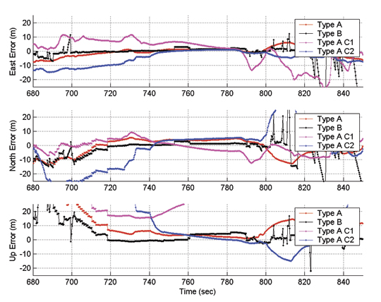
The RTK service was established during the spring of 2010 and was run in test mode May 12–July 31 to test system accuracy, signal coverage area, and signal availability.
Accuracy. An error budget of the RTK service is provided including all known error sources and latencies in the system, and a description of how these errors are handled. The accuracy obtainable by end users is better than 1.0 centimeters in the horizontal and better than 1.8 centimeters in the vertical. Values are provided as one sigma, and are valid during normal ionospheric activity. Applying an RTK rover and RTK corrections received from the FBPS RTK service, users inside the coverage area can determine the coordinates of a marked survey point repeatedly with these accuracies.
System inspection is carried out monthly. Part of monthly inspection is the visit of marked control points with an RTK rover. ISO 17123-8:2007 (ANSI, 2007) standard procedures are applied to determine control point coordinates.
Coverage Area. The RTK service coverage area shown in Figure 5 is defined as the geographic area where the described accuracy can be obtained for end users at any time. Test measurements of UHF radio signal strengths from the four primary GNSS stations have been carried out onshore Lolland and Fehmarn, as well as offshore across the Fehmarnbelt (see photo). Modelled UHF radio signal broadcasting areas are closely verified during these tests.
Availability. The positioning system and the RTK service are designed using necessary technology, redundancy, and back-up to ensure that the system is operational and available in the entire coverage area for more than 99 percent of the time. Availability is defined as the time where all elements of the positioning system are available for end users and where the described accuracy can be obtained for all users within the coverage area. Availability is evaluated in percent of time per day: the system must be available for at least 23 hours and 45 minutes per day. During the first year of operation it is accepted that RTK correction data from the system are available to end users for 97 percent of the time or more per day.
A control segment has been established to constantly monitor RTK service accuracy and the availability of the system. The control segment is installed in such a way that all relevant output and data streams from the GNSS stations are available through the system’s website.
Evaluation of availability is carried out automatically by the control segment, and an overall evaluation of availability is performed every month. Results from evaluation of availability during the test operation are listed in Table 2. During test operation, the required availability of 97 percent per day during the first year of operation was reached on all days. Availability only fell below 99 percent, as is the required availability during following years, for 5 out of 81 days (5.6 percent) of the test period.
Conclusions and Outlook
System tests results regarding accuracy, coverage area, and availability show that the positioning system and the RTK service fulfil all specifiecation requirements.The first RTK user was registered in July 2010, and the complete system is now being used for environmental, geotechnical, and geophysical investigations.
User benefits of the FBPS include:
ensured consistent and uniform geodetic reference throughout the planning, construction and operation phases of the Fehmarnbelt Fixed Link, available to all stakeholders at any time;
seamless, real-time data flow from the point measurement at the construction site into computer-aided design (CAD) or geographic information systems (GIS);
simplified geodata transfer across interfaces between project stakeholders and project phases;
cost efficiency, reducing costs in both surveying and data management, particularly in precise operation of large, expensive offshore equipment, including during critical procedures in the construction phase.
The positioning system for the Fehmarnbelt Fixed Link is an example of a homogeneous, consistent, coherent, and highly accurate GNSS-based positioning system. Comparable systems and services can be established and used for any major construction site or infrastructure project.
Acknowledgments
This work is funded by Femern A/S. The authors acknowledge contributions from the National Survey and Cadastre, Denmark, Danish National Space Institute, Land Survey Office of Schleswig-Holstein in Germany, German Federal Agency for Cartography and Geodesy, Richter Deformationsmesstechnik GmbH, Günther Steimann, and Ohms Nachtigall Engineering GbR. Also Mr. and Ms. Thomsen, Stadt Fehmarn, Mr. Henriksen, and Mr. Boserup for permitting establishment of FBPS GNSS stations on their property.
Establishment, operation and maintenance of the GNSS stations and RTK service was entrusted by Femern A/S to AXIO-NET GmbH, with ALLSAT as subcontractor for implementation of the four GNSS stations (both companies in Hannover, Germany). Ramboll Arup JV was entrusted by Femern A/S with project coordination and geodetic consultancy, using AJ Geomatics as subcontractor. More information about the fixed link is available, and more on the RTK service.
Manufacturers
The RTK service is based on GNSMART software (GEO++ GmbH). The permanent GNSS stations are equipped with Leica Geosystems AR25 antennas and GRX1200+ receivers.
Anna Jensen is owner and CEO of AJ Geomatics in Denmark. She holds a Ph.D. in geodesy and has worked with research and development within GNSS and geodesy for more than 15 years.
Dirk Hermsmeyer holds a Ph.D. from the University of Hannover, and is a project management professional. He previously worked at ALLSAT and is now with the Chamber of Commerce in Lübeck, Germany.
Bastian Huck is head of operations and quality management with AXIO-NET. He is a university-level geodesist and certificated project management practitioner with 10 years of experience in RTK projects.
Jürgen Rüffer is co-owner and CEO of ALLSAT and AXIO-NET. He is a university-level geodesist, a publicly certified expert for GNSS positioning at the chamber of engineers in Germany, working with GPS and GNSS since 1977.
Peter Skjellerup is chief advisor on geotechnology with Ramboll Denmark. He has worked with ground engineering for many years, and holds a M.Sc. in physics-geophysics from the University of Copenhagen.
Note from author Anna Jensen (2/27/13):
“Since publication of the article, the opening year for the Fehmarnbelt tunnel has been changed to 2021.”
By Dinesh Manandhar and Hideyuki Torimoto, GNSS Technologies, Inc. Japan
An indoor messaging system (IMES) has been developed to meet the challenges of indoor and deep indoor positioning, as a system that can be implemented in any device that has a GPS/GNSS receiver without hardware modification. IMES can provide reliable 3D position data with a single transmitter device without performing range calculation.
The cost of embedding location data in portable electronic devices is so low that universal penetration can be foreseen in the next five years. Roughly 70 percent of the world’s population now uses approximately five billion cell phones. This number has doubled in the last four years. Future growth is expected at the same or even a higher growth rate.
Due to the emergence of smart phones and location-based services (LBS), mobile phones are used not only for communications but also for many applications related to LBS, entertainment, and games. GPS/GNSS devices are included in mobile phones due to compulsory requirement of E911 and safety-and-rescue services by law in many countries for security and safety.
Access to map data and value-added services using these map data is getting cheaper and eventually will be freely available. Major service providers like Google, Nokia, and Apple already provide access free of cost, and they increasingly focus on location as a core business construct.
GPS/GNSS devices were designed to work outdoors, and most GNSS applications are limited to outdoor environments. However, GNSS reliability, availability, and accuracy have led to development of many new and innovative applications that are designed for use in both outdoors and indoors in a seamless fashion. Today, GNSS receivers are integrated in many other devices like mobile phones, navigation systems, personal navigation devices, game devices, security devices, and many LBS-related devices. These devices are increasingly used in indoor environments. Indeed, people generally spend much more time indoors than outdoors. Hence, it is extremely important to have a reliable system that can provide fairly accurate position data even in indoor and deep indoor locations.
Current GNSS systems do not provide solutions for indoor and deep indoor environment with reliable accuracy of 10–20 meters. New modernized signals such as L5 do provide better position accuracy and better signal reception in indoor areas, but achievable positioning will still vary, and will continue to require more than four visible satellites with some assist data — and still be limited to soft indoors environments such as rooms with glass windows or walls. Limitations remain for hard and deep indoor environments.
To surmount these obstacles and provide indoor navigation, various technologies such as pseudolites, assisted GPS, wireless networks (Wi-Fi), Bluetooth, RF tagging, and so on have been developed. However, these technologies have their own limitations and are not the most suitable tools for seamless positioning and navigation. Except for pseudolite and A-GPS, they are designed for communication, not for positioning or navigation purposes, but are used for navigation purposes since no other suitable technology exist.
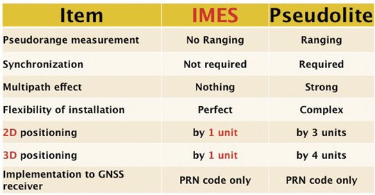
Pseudolite systems are currently in use for indoor positioning. While technically sound, a system needs at least four signal transmitting units. To cover a large area, it needs many transmitters suitably located and time-synchronized to one other, or their clock errors must be known. Pseudolite systems provide position data based on range calculation from the receiver to a number of transmitters, and this calculation is heavily affected by signal multipath. Table 1 compares IMES and pseudolites.
Table 1. Comparison between IMES and pseudolite.
A-GPS is widely used in mobile phones to compute position data. A-GPS technology includes high-sensitivity signal processing to acquire weak signals and external assistance of data like time, approximate position, and satellite-orbit related parameters. Provision of assistance data requires a communication link between the receiver and the data source, for example, the mobile phone network itself. Thus, A-GPS will not be possible if there is no communication link.
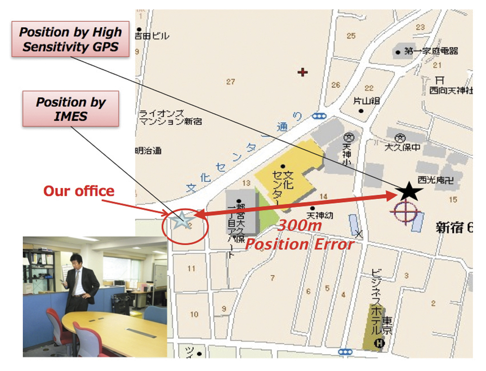
Normally, A-GPS provides 2D position data. The height data (if 3D output is available) will be highly erroneous. The accuracy of such position data varies from few tens of meters to few hundreds of meters. Also, the position data is heavily affected by signal multipath. Figure 2 compares IMES position and mobile phone position inside an office building. The A-GPS position error is about 300 meters in this case.
FIGURE 2. Indoor position from high-sensitivity GPS and IMES.
Wi-Fi is used for indoor positioning in many mobile phone devices. The phone provides position data from a built-in GPS receiver, a Wi-Fi device, cell ID, or a combination of any of these. Recently, position data from Wi-Fi has become popular for indoor as well as outdoor position, since Wi-Fi signals are so freely available. However, using these Wi-Fi signals requires registering the signal power and availability at reference locations. To do this, a huge number of Wi-Fi devices are registered driving around the city. Since these devices are basically installed for communication purposes, they can be relocated, removed, or new devices may be installed without any information to the users or service providers. Thus, continuous maintenance and updating of all these devices are necessary at certain time intervals. The coverage of Wi-Fi devices is not uniform and may vary widely from area to area, affecting position accuracy.
Telecom service providers are considering the possibilities of seamless positioning technologies. They would like to have one single device that can provide 3D position data both indoors and outdoors, without additional power or cost, and with satisfactory 3D position information. If such a seamless positioning technology is available, it will undoubtedly generate a huge global commercial market. The availability of such technology will also aid development of new applications in location-based services, advertising, marketing, entertainment, and gaming.
We have conducted research in indoor positioning for the past few years, beginning with pseudolite systems. We have developed IMES to meet the shortcomings of the technologies described earlier for indoor and deep indoor positioning. IMES for a seamless positioning environment can be implemented in any device that has a GPS/GNSS receiver, without hardware modification. IMES can provide satisfactory and reliable 3D position data with a single transmitter device without performing range calculation.
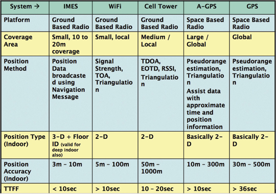
Table 2 compares IMES with other indoor-position capable devices. IMES can provide the same accuracy even in deep indoor locations, whereas cell tower, A-GPS, and GPS cannot work in such areas. All other systems except IMES provide only 2D position data indoors. The height data from A-GPS is very unreliable and hence cannot be used.
Table 2. Comparison of IMES with other indoor positioning systems.
IMES Concept
The main concept of IMES is to transmit position and floor ID of the transmitter with the same RF signal as GPS. IMES transmits latitude, longitude, height, and floor ID by replacing the ephemeris and clock data in the navigation mes
sage of GPS. A single unit of IMES is enough to get the position data, since the position itself is directly transmitted.
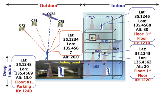
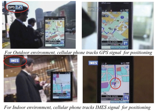
Figure 3 shows the concept of seamless position data using IMES, where the same receiver can be used both indoors and outdoors without interruption. GNSS satellites provide positioning and navigations outdoors, while IMES provides indoor navigation. Since the signal structures of GPS satellites and IMES is the same except for the navigation message contents, the same receiver can be used for both cases. Current GPS receivers will be capable of receiving IMES signals with modification of firmware only to decode the navigation message. Figure 3shows the concept of seamless 3D route guidance.
Figure 3. Seamless 3D route guidance using IMES.
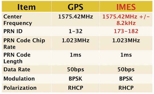
Signal Properties. The IMES signal is designed much like the GPS signal. It uses the same center frequency as GPS with an offset of +/– 8.2 kHz to minimize the possible interference from IMES to GPS signal. Ten PRN codes from 173 to 182 are assigned for IMES. These codes are provided by the U.S. government. Other signal-related parameters are the same as the GPS L1 C/A code signal. Table 3 shows IMES signal properties with respect to the GPS signal.
Table 3. IMES signal properties with respect to GPS.
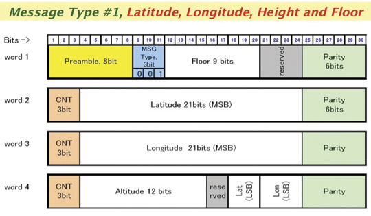
IMES has four different types of navigation message. The most significant is Type 1 as shown in Figure 4. It transmits latitude, longitude, height, and floor ID. The transmission of floor ID is a key factor for perfect 3D position data. Other message types are Type 0 (2-D position data with floor ID), Type 3 (short ID), and Type 4 (medium ID).
Figure 4. IMES Message type 1, 3D position, and floor
Interference Issue
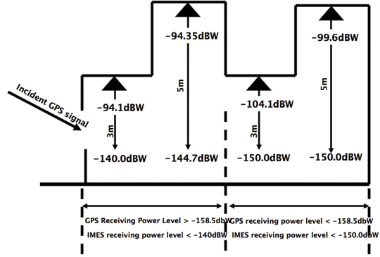
Since IMES shares the same frequency as GPS L1 band (1575.42 MHz), there is an interference level that IMES may have on GPS signals. This interference has been studied in detail by conducting experiments and simulations. Based on these studies and analysis, various methods have been considered to avoid harmful interference to GPS signal. To avoid such interference, IMES center frequency is shifted by +/– 8.2 Khz from GPS L1 band. This will have the least impact on the GPS L1 band signal. For example, if the IMES signal is –110 dBm (very strong) and the GPS signal is –142 dBm (very weak), the loss of GPS signal (C/N0) due to IMES is less than 2 dB. If the IMES signal is –120 dBm and the GPS signal is –142 dBm, there is no loss of GPS signal (C/N0). Based on this analysis, the IMES transmitter power must be controlled such that the maximum power to the receiver does not exceed –110 dBm at a distance of 3 meters from the transmitter. Figure 5 shows the guideline specified in the QZSS IS document for setting the transmitter effective isotropic radiated power (EIRP)based on location.
Figure 5. IMES transmitter power setup guideline in QZSS IS document.
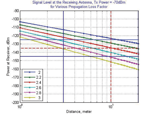
Figure 6 shows the signal propagation loss for transmitter power of –70 dBm for various propagation loss-factor values of n. Figure 7 shows path loss for various transmitter power for the same loss factor, n = 2.5. These graphs shows the maximum power that shall be used to cover an area without exceeding the maximum power level. If a single unit of IMES cannot cover the complete area, then multiple IMES units will be deployed to cover the entire area with suitable power level. These graphs serve as a guideline for setting transmitter power.
Figure 6. Signal path loss for –70 dBm signal for different path loss coefficient, n.Figure 7. Signal path loss for path loss coefficient, n = 2.5, for different transmitter power levels.
The signal propagation loss is calculated using the following equation; the gain of transmitter and receiver antennas is considered as unit gain (0 dB).
Hence, the equation depends on distance from the transmitter, d, and the propagation loss factor, n. The value of n is 2 for free space and increases for areas with objects that obstruct the signal. An office with soft partitions may use n = 2.5. The graphs can be used as a guideline to estimate the transmitter power to cover an area within the allowed power levels.
Application Areas
IMES can be used wherever indoor position data is required. It depends upon the application for that particular location as well. For example, an infrastructure-related safety application should have IMES installed at all elevators, escalators, staircases, emergency exits and routes, fire-fighting unit locations, and so on. Here are some of places where IMES might be used:
Every room of a building, to provide exact room location.
At entrances, exits, elevators, escalators, staircases, public facilities, and corridors for indoor navigation.
At every emergency exit for guidance.
Along hallways and lobbies at set intervals to guide the user.
In front of shops for advertising and information.
In sign posts to provide user’s location and guidance.
Complement other positioning systems like Wi-Fi, RF Tag, UWB, and so on.
As an indoor ground control point for surveying of large and multi-storey buildings.
With security cameras to provide accurate position data.
In factory production lines for automated control of moving objects.
Business Perspective
IMES technology was developed with the guiding concepts of low-cost global implementation and ease of installation and use. Low cost on the transmitter side is achieved by developing large-scale integratin (LSI) chips and IMES installation, setup, and database management tools. At the receiver side it is achieved by design of IMES signal so that existing GPS receivers in mobile phones, PDAs, or any other devices can use IMES by modifying only the firmware. The signal is designed so that it can adapt to other GNSS signals available in the future, for example, Galileo, QZSS, or Compass signals, requiring only firmware modification. Global implementation is made possible by signal design compatibility with existing GPS or GNSS signals. Ease of use is achieved again by signal design: one IMES transmitter can provide 3D position data, including floor information, with reliability and accuracy of a few meters even in deep indoor locations.
The development of IMES LSI chips (IMES transmitter) will also lead to development of value-added products for many consumer household appliances. For example, the green energy concept produced low-power LED lightbulbs. IMES chips can be installed in LED bulbs at very low additional cost. Similarly, it can be built in many other products like power socket devices, security devices, timing devices, and sensors where position data is also critical. This will provide an opportunity for the manufacturers to provide value-added products to users with indoor positioning devices. Not only electrical products but some construction materials or interior decoration materials like gypsum (dry
wall) boards can be made with built-in IMES chips. Installation of one piece of wallboard with an IMES built-in chip can provide position data in the room, reducing installation cost while not affecting the interior design of the room.
Implementation of IMES will also lead to new applications in the field of location-based services and applications where position data are necessary. It can also lead to new applications using IMES as an indoor electronic ground control point (GCP) in large buildings and indoor areas.
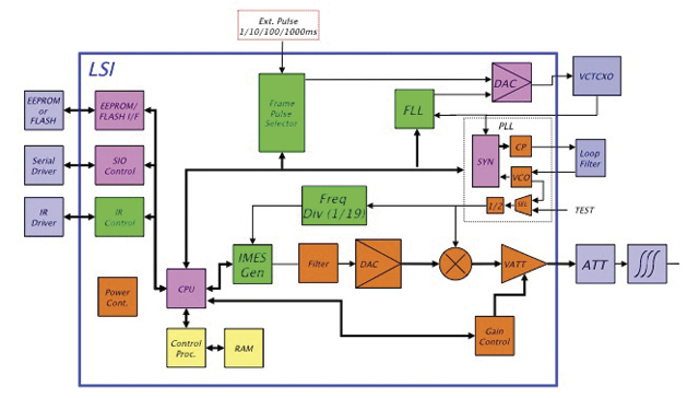
Chip Development. To reduce IMES transmitter cost, the IMES LSI chip has been developed and will be available by the end of the third quarter of 2011. This will reduce overall cost and size, and create platforms to develop value-added products integrating with other devices and systems. The chip is designed for global communications systems like personal handy-phone system (PHS, a mobile phone communication system developed in Japan), CDMA, and GSM. Figure 8 shows a block diagram of the chip transmitter.
The basic specifications of the LSI chip are: size, 12 x 12 millimeters; power, to be determined; maximum transmit power, –30 dBm or –60 dBm (user selectable); frequency, L1 band, 1575.4282 MHz or 1575.4118 MHz (user selectable); PRN codes, 173–182 (user selectable); signal type, GPS L1C/A, with upgrade capability to other GNSS signals.
Installation and Management
An IMES installation, setting, and management system has been developed to facilitate deployment. The main purpose of the system is to provide IMES transmitter position data (latitude, longitude, height) without conducting precision surveys, thus reducing installation, setting, and management costs. The system helps locate optimum locations for IMES transmitter siting, control transmitter EIRP power, set PRN IDs, and assign position data. The system can also use various types of map data sources to generate necessary floor data or indoor maps in 3D. The inputs can be either 3D vector data or 2D raster images, or even paper maps.
The overall system consists of four sub-systems:
IMES Setup Tool (ISET). This tool is used to set up the IMES transmitter. It provides two basic functions: to set up signal-related data (setting PRN code, transmitter power, navigation message rate, and so on) and to set up message-related data (position data, floor data, message types and their contents, message sequence, and so on). The R&D version of IMES also allows transmitting some special data for research and development purpose. It is possible to change the preamble value different from GPS, load a different PRN code table than IMES, change the navigation message data rate, generate a BOC(1,1) signal to test L1C-like signals, and change the RF frequency. The setup tool also has user-access management so that only authorized users can change certain sensitive data like PRN code, position data, and transmitter power.
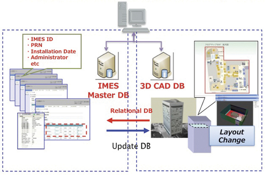
IMES Database Management Tool (IDBM). This tool simplifies installation and management by providing a necessary database including a building-related database, a service-provider database, a device-related database, other integrated sensors database (if any), and a signal-related database. Since IMES is controlled and managed, guaranteed and authorized services can be provided for dedicated applications. This enhances the reliability of an IMES-based positioning system for infrastructure, security, and safety-related applications.
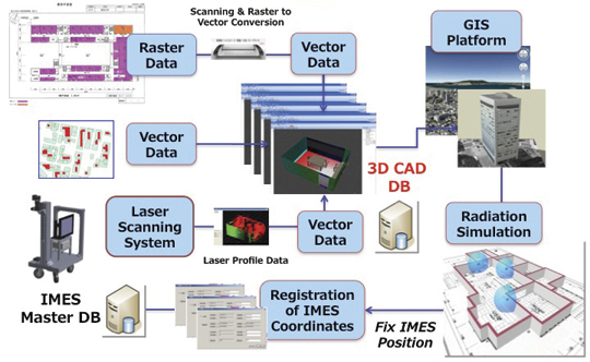
3D Mapping Tool (IMAP). This tool, shown in Figure 9, provides a 3D map database for IMES either for implementation or end-user applications. The mapping tool can use 3D vector data (for example, existing DXF files), raster image data, or direct user input. A laser scanning system with CCD camera is used to generate 3D data if existing data is not available. The tool creates walls, windows, doors, ceilings and other smaller objects from the laser data. If data are available in paper drawings, they are scanned to create raster images before digitizing them into vector format.
Figure 9. 3D Map Database Development System.Figure 10. Concept of IMES database for implementation, setting and management.
The system will ultimately create a 3D database of a building at floor level that can be linked with external databases. Figure 10 shows the overall concept of the IMES database system that includes both IMES database and 3D map database. The two database systems are linked by a relational database system. Any update in the map database can be reflected into the IMES database.
Signal Propagation Loss Tool (IPMODEL). This tool simulates the signal level where IMES will be set up. It is necessary to have optimum deployment of the transmitter to cover the area as large as possible within the allowed power level. Although the allowed maximum EIRP power level is –64 dBm for Japan, the approach is always to use the least power possible to cover the area, to avoid any possible harmful interference to other systems as well as to limit the availability of the signal to only the desired area.
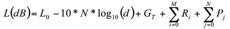
The following equation is used to calculate the signal path loss which is based on Frii’s free-space path-loss model.
GT is the transmitter antenna gain. The receiver antenna gain is assumed to have unit gain (0 dB) and hence not included in the model.
L0 is the power loss at 1 m distance and is given by 20 x log10(signal wavelength) — 20 x log10(4*pi).
N is the path-loss factor, which is 2 for free space, 2.5 for office room with soft partition, and 3.0 for rooms with hard partition.
Ri is loss due to i number of reflections by objects.
Pj is loss due to j number of penetrations through objects.
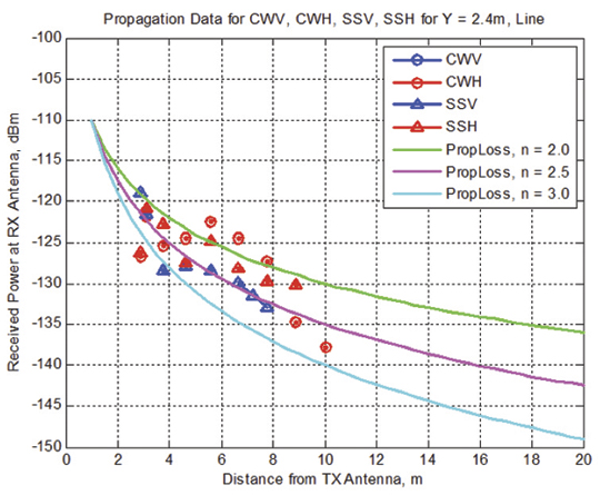
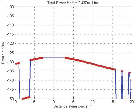
Figure 11 shows the propagation-loss tool flowchart. It uses 3D map database provided by the 3D mapping tool and database from the database management tool. It also uses antenna gain pattern and material electrical properties to compute the power loss due to reflection and penetration. Figure 12 shows the signal propagation output from the model for a building lobby. Figure 13 and Figure 14 show the output from the propagation loss results from the actual measurement and model output, respectively. The results match within a difference of few dBs.
Figure 11. Path Loss Tool flowchart.Figure 12. 3D view of signal power in a building lobby.Figure 13. Actual signal power measured at different locations in the lobby shown in Figure 12Figure 14. Signal power output from the propagation loss tool at the same location shown in Figure 13
Experiments and Demonstrations
Experiments and demonstrations have been conducted to validate the IMES concept, uses, and applications. Early experiments validated the
concept, message design, and interference analysis. Later experiments focused on actual implementation for infrastructure, and social-network and location-based applications. Pilot projects have been conducted in collaboration with the Japanese government to test IMES capabilities for seamless positioning and navigation and for social infrastructure platform.
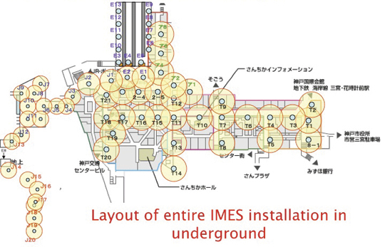
The Free Mobility Project in Kobe is the biggest social experiment using IMES for seamless navigation under the sponsorship by the Ministry of Land, Infrastructure, Transport, and Tourism. The project was conducted in an underground shopping mall of Kobe railway station. Shopping mall visitors were asked to participate in the navigation using IMES-capable mobile phones. Most visitors could follow the route they had chosen or find the destination point using the IMES set-up.
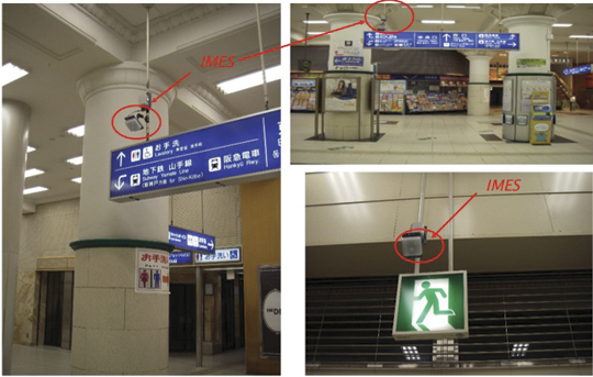
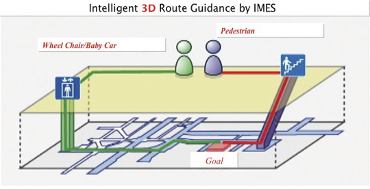
A total of 70 IMES transmitter units were installed at locations including ticket counters, elevator entrances, emergency exits, fire-extinguisher locations, staircases, station entrances, and alleys of the shopping mall. Figure 15 shows a part of the IMES transmitter location map. It covers one of the sections of the shopping mall. Figure 16 shows various locations where IMES transmitter devices were installed. As shown in Figure 17, intelligent 3D route guidance can be performed based on user preference. For example, a user in a wheelchair must be guided by a route that has no staircases, shown by green route in the figure, to reach the destination. A pedestrian can be guided by red route, which is the most direct route to the destination.
Figure 15. IMES transmitter location map to cover the underground shopping mall in Kobe Station.Figure 16. Installation of IMES near the station entrance and emergency exit.Figure 17. Intelligent 3D route guidance using IMES.Figure 18. Seamless navigation by mobile phone using GPS and IMES.
The distribution of each IMES transmitter is done in such a way that it covers a radial distance of 10 to 20 meters. The deployment density of IMES depends on the location environment. If an IMES device is located near the entrance, the coverage distance will be around 10 meters to minimize transmitted power. IMES devices in deep indoor locations can cover a radial distance of about 15 to 20 meters.
Commercially available mobile phones with a firmware update for IMES were used to receive the IMES position data. The phones also included the shopping mall and station map including related databases for various applications.
Conclusions
IMES can provide reliable and guaranteed 3D position accuracy, including floor information. IMES signal design is done in such a way that it can use existing as well future GPS/GNSS receivers without any hardware modifications. Necessary implementation, setup, and management tools are also developed to facilitate IMES installation and to minimize the cost so that large-scale global implementation is possible. IMES LSI chips are being developed for large-scale implementation. IMES will also help in developing many other location-based applications and services. IMES evaluation kits will soon be available for joint R&D projects.
IMES technology-related patents have been filed in Japan and many other countries. The basic patents have already been approved in Japan. GNSS Technologies invites academic institutions to participate in joint R&D projects.
Dinesh Manandhar is a visiting researcher at the University of Tokyo, where he received his Ph. D, and a senior researcher at GNSS Technologies Inc. He is one of the designers of IMES message structure and involved in developing indoor navigation system based on IMES for seamless navigation environment. He can be reached at [email protected].
Hideyuki Torimoto is the president of GNSS Technologies Inc. Japan. He established Trimble Navigation Japan and Weathernews Inc. in 1986. He also established the Research Forum on Social Infrastructure for Advanced Positioning (NPO) in 2003 and the Satellite Technology Laboratory in Tokyo University of Marine Science in 2004. He served as Satellite Division Member of ION for 2003-04. He can be reached at torimoto @ gnss.co.jp.
The European Satellite Navigation Competition (ESNC) — also known as the Galileo Masters — is looking for applications based on satellite navigation that use the technology in a new and innovative way. The deadline for entering is June 30.
No matter whether you are an individual or a team from a company, research institute, university, or start-up, what counts is your idea, say organizers.
The competition began in 2004 with three partner regions. Since then, the ESNC has grown into a global network of innovation and expertise, say organizers. In 2010, 23 regions competed against one another, 548 participants registered, and the 357 ideas turned in were evaluated by 186 experts. Many of the ideas submitted in previous years have been implemented and successfully launched into the market, according to the Galileo Masters team: "The key to our success is close collaboration with regional, institutional, and industrial partners with whom we share one common goal: promoting innovation and entrepreneurial spirit on Europe’s GNSS markets."
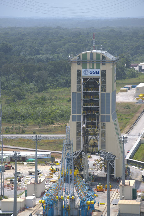
The ESA announced the Soyuz site at Europe’s Spaceport in French Guiana is now ready for its first launch. ESA yesterday handed over the complex to Arianespace, marking a major step towards this year’s inaugural flight.
According to the announcement, construction of the Soyuz site began in February 2007, although initial excavation and ground infrastructure work began in 2005 and 2006, respectively. Russian staff arrived in French Guiana in mid-2008 to assemble the launch table, mobile gantry, fuelling systems and test benches. The first two Soyuz launchers arrived from Russia by sea in November 2009 to be assembled in the new preparation and integration building.
Soyuz mobile gantry.
The French space agency, CNES, as prime contractor for the building work, along with its European and Russian partners, has spent recent months qualifying the site – known as Ensemble de Lancement Soyuz, or ELS for short. The tests covered all the mechanical, fluid and electrical elements, such as the pad’s umbilical arms and fuelling vehicles, and all the buildings, including the launch control centre that will house the combined European and Russianteams.The ‘acceptance review’ this week declared that the site is ready for its first rocket. At the same time CNES handed over the facilities to ESA.
The last step this week was ESA’s hand-over to Arianespace.
According to the announcement, the launch site is almost identical to the other Soyuz sites in Kazakhstan and Russia, although adapted to conform to European safety regulations. The most visible difference is the 45 m-tall mobile gantry, which provides a protected environment as payloads are installed on the vertical launcher. Its internal movable work platforms provide access to the Soyuz at various levels.
The ESA reports that from now on Arianespace is responsible for the Soyuz launch site and will begin the campaign this month to qualify its launch operations. A launch rehearsal will ensure that the Soyuz and the new facilities work together perfectly, while allowing the teams to train under realistic launch conditions. This simulated launch campaign will include the vehicle’s transfer to the launch zone, its erection into the vertical position, its installation on the pad, and the testing of ground and launcher interfaces. These final tests will give the green light for the first Soyuz flight from French Guiana in the third quarter of 2011.
By Oscar Pozzobon, Chris Wullems, and Marco Detratti
Modern GNSS will provide access control to the signal through spreading-code encryption and/or authentication at the navigation data level. This will require support within the receiver for secure cryptographic keys and the implementation of security functions. This article reviews vulnerabilities of these security functions, and reviews design considerations to mitigate attacks.
The threat of spoofing attack on GNSS has led to the design of signals and receiver technologies addressing this problem at signal, data, and receiver levels. Transportation, governmental, financial, and access-control applications demand trusted position velocity and time. Security functions in the receiver require implementation of cryptographic functions and key storage in the receiver. We can distinguish three uses of cryptographic keys and functions:
signal access control;
navigation data authentication and access control; and
position, velocity, time, and signal authentication state privacy and integrity.
The need to protect the cryptographic functions and keys, software, hardware, and data communication of next-generation secure GNSS receivers against attacks is imperative, to prevent signal spoofing and signal and position access to an hostile party. Here we provide guidelines that can support the design of tamper-resistant GNSS receivers.
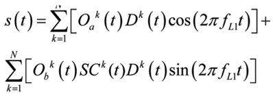
Signal access control is achieved through spreading-code encryption. The spreading sequence is encrypted with a stream cipher, and the receiver needs the key in order to locally reproduce the signal and perform operations of acquisition and tracking. If the stream cipher frequency is considerably lower than the original code chipping rate frequency, such as the GPS W-code with respect to the P-code, other codeless and semi-codeless techniques can be used for signal tracking. However, these techniques lie outside the objective of this study that will focus on the need for keys to decode the signal, and the requirements to protect them.
Direct sequence spread-spectrum (DSSS) access-control schemes can be implemented with a binary-stream cipher that acts as pseudorandom spreading sequence, or the spreading sequence can be modulo 2 summed to a stream cipher at the same or different frequency. The encryption module in the transmitter needs the key and initialization vector (IV) to perform the encryption operation. It is assumed that the transmitted signal (neglecting signal amplitute) will be:
(1)
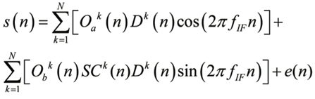
where Oak and Obk are the publicly known spreading codes such as the C/A and P-code of GPS for every K satellite, SCk is the is the stream cipher (W code for GPS) and Dk is the transmitted data. After the AD conversion the signal will be:
(2)
where e(n) is the thermal noise introduced in the sampling process.
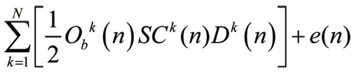
After the carrier removal by multiplication with sin (2π fIFn) to obtain the quadrature arm containing the encrypted signal, and after the application of a low-pass filter to cut the 2π (2 fIF) frequency, the remaining signal for every satellite is:
(3)
The encryption module in the receiver needs the key and IV to recreate the local signal and perform code acquisition and tracking. Cryptographic keys in GNSS are assumed to be secured in the ground and space segment, and the ground control center performs operations of key loading to the satellites. However, key loading to the GNSS receiver is a sensitive operation. An adversary might obtain the keys and use them to access the encrypted signal in other receivers.
A malicious key recovery could be used to generate false encrypted signals, leading to a risk of signal spoofing. Key loading to the receiver can be achieved with a public key encryption and public key infrastructure, where the stream cipher key and IV are encrypted with the receiver public key, and only the receiver private key can decrypt the cipher key and IV.
The receiver private key and stream cipher key must be protected by a tamper-resistant module to prevent attacks. Figure 1 shows a high-level block diagram of a GNSS receiver with functions to access encrypted codes. There are two areas to be protected, depending on the security objectives:
Limit access of the signal to a restricted group: prevent signal spoofing. The red blocks shows the critical components to protect these objectives, including the storage of the secret keys, the stream cipher generation, and the final local secret code (LSC) replica (4) which is a noise-less signal from which the stream cipher can be easily obtained by modulo 2 sum of the local not-secret Obk code (5).
(4)
(5)
The red blocks should be protected in order to avoid key recovery or cipher stream analysis by an attacker.
Figure 1. Signal access control sensitive blocks.
Control access to Position, Velocity and Time (PVT). The yellow blocks show the critical components that should also be further protected in order to limit the PVT access. The tracking functions provide information such timing and pseudorange measurement that can be used for positioning, and the communication line should be protected. The navigation processing block performs the position and time solution, and the access to the data shall be protected.
Data Authentication, Access Control. A system might provide access control and authentication to the navigation data only. In such a design, the spreading sequence is publicly known, while the data is encrypted or contains authentication messages. The security objectives can be distinguished as:
◾ Access control to data of the acquisition and tracking functions. If fundamental parameters for the position solutions are encrypted (such as transmission time and satellite position) and therefore unavailable, a GNSS receiver could attempt the PVT solution with standard approaches. Therefore the Navigation Message Encryption (NME) restricts the access of PVT only to the user group that has the cryptographic keys for the navigation message decryption.
◾ Navigation Data Integrity. Navigation data can be authenticated (with cryptographic authentication schemes such as Message Authentication Schemes [MAC] or digital signatures). The objective of Navigation Message Authentication (NMA) is to provide an enhancement to the integrity of the messages towards intentional attacks. Such design can be an option in order to reduce the signal spoofing risk, as an attacker needs to rely on the messages (with a receiver-spoofer architecture for example).
Figure 2 provides an high-level architecture of a GNSS receiver block diagram that supports NMA and/or NME. The red blocks shows the sensitive parts that must be protected. In case of NMA the key that verifies the integrity (for example, a public key certificate) must be stored securely to avoid an attacker substituting the key and spoofing the navigation data with alternative keys (for example, the root CA could be stored in ROM). A trusted clock component is included in the diagram, as it can be an interesting option to consider in order to avoid NMA spoofing attacks.
Figure 2. Schematic of assistance solution.
PVT and Signal Authentication State Integrity and Privacy. Many applications require a PVT integrity to be cryptographically verifiable. Applications that require secure tracking systems (anti-theft, hazmat tracking, road toll, navigation statistics for insurance companies) and information security applications based on GNSS (location-based access control and geo-encryption) require PVT integrity. It is trivial to tamper with the data communication between a GNSS receiver and a final application (for example, interfering with the serial output of the chipset) and generate false PVT, in a data-spoofing attack. In Figure 2 the cryptographic keys used to add integrity to the PVT messages are typically different from the keys used for NMA or NME, and are application-specific. Such an architecture could be also the choice for differential corrections authentication, where the navigation processing block could verify the integrity of the correction data before aiding the position solution algorithm.
Attacks on Security Functions
This section identifies attacks that can compromise the functions of the previous section. Attacks to the signal are not pertinent to this work. We distinguish the attacks in two main categories: physical attacks and side-channel attacks. Among physical attacks, we distinguish:
Microprobing. This refers to techniques that attempt to access the physical components of GNSS receiver such as the baseband processor and RAM/ROM memory chip surface to observe and manipulate sensitive data. A microprobing attack can be targeted to recover the cryptographic keys.
Focused Ion Beam. FIB is a technique for deposition and ablation of materials in semiconductors, where chip material can be removed with micrometer resolution. It consists of a vacuum chamber with a particle gun. FIBs are used by attackers for manually probing the signal of interest. A micrometer hole is created to reach the signal of interest and filled with platinum, terminating with a pad. The signal can then be connected to an external probe.
Software Attacks. These happen through vulnerabilities of the communication interface or security protocols, or through malicious firmware upgrades in the baseband processor.
Eavesdropping Techniques. These monitor sensitive communication lines (such as baseband to HW correlator where the spreading code could be observed).
The most common side-channel attacks are timing, power, and fault analysis, in which an attacker seeks to exploit side-channel information in order to recover a cryptographic key. The most effective mitigation strategy against such attacks is to design and implement the cryptosystems with the assumption that information (time and power) will leak. Different types of side-channel attacks and their respective countermeasures are:
Fault-Generation Techniques. These are used to investigate ciphers and extract keys by generating faults in the system, either by intentionally causing faults or by natural faults that occur. Faults can be most often caused by changing the voltage, tampering with the clock, changing temperatures, and applying radiation of various types.
Timing Analysis. This class of attack allows cryptanalysts to extract keys by analyzing the time taken to execute cryptographic algorithms. Every logical operation in a computer takes time to execute, and the time can differ based on the input; with precise measurements of the time for each operation, an attacker can work backwards to the input.
Simple and Differential Power Analysis. SPA or DPA is a class of attack that allows cryptanalysts to extract secret keys and compromise the security of smart cards and other cryptographic devices by analyzing their power consumption. Differential power analysis attacks use statistical analysis and error-correction statistical methods to obtain information about the keys.
Electromagnetic Radiation Analysis. This is concerned with the monitoring/recording of radiation for the purpose of obtaining information about the operation of associated hardware, which could be used ultimately to determine cryptographic keys. Fluctuations in current generate radio waves, making whatever is producing the currents, in principle, subject to a van Eck (TEMPEST) attack. If the currents concerned are patterned in distinguishable ways, which is typically the case, the radiation can be recorded and analyzed in order to infer information on the operation of such hardware.
Acoustic Analysis is concerned with the observation of the acoustic emissions from a chip in order to obtain information about the code being executed. Information about the operation of cryptosystems and algorithms can be obtained in this way. Flowing currents heat the materials through which they flow. Those materials also continually lose heat to the environment due to other equally fundamental facts of thermodynamic existence, so there is a continually changing thermally induced mechanical stress as a result of these heating and cooling effects. That stress appears to be the most significant contributor to low-level acoustic (that is, noise) emissions from operating CPUs. If the surface of the CPU chip, or in some cases the CPU package, can be observed, infrared images can also provide information about the code being executed on the CPU, known as a thermal imaging attack.
Mitigation Strategies
We derived several design considerations to mitigate attacks from our experience during the development of the Trusted Innovative GNSS rEceiveR (TIGER) project. The TIGER is a tamper-resistant GNSS receiver which provides PVT integrity, signal spoofing and jamming detection, and signal state attestation with an open GNSS signal.
Cryptographic subsystem. This is designed for resistance against timing-based attacks. Timing-based attacks targeted to the cryptographic module can be prevented by careful implementation of the cryptographic functions. A non-exhaustive list of countermeasures that can be considered for mitigation of timing-based attacks includes:
Ensure that the time a cryptographic operation takes is independent of the input data or key bits. These operations should take the same number of clock cycles.
Ensure that the software implementation of critical code does not contain conditional branches (i.e., IF statements). Functions should use operations such as AND, OR, or XOR instead .
Ensure time taken for multiplication and exponentiation is the same, such that an attacker cannot learn how many multiplications and how many exponentiations have been performed. A simple method is to always perform both multiplication and exponentiation.
Addition of delays such that all operations take the same amount of time, although this can have a detrimental effect on performance. The addition of random delays can increase attack difficulty.
Protection from Electronic Level Interception/Monitoring. One approach for mitigation of microprobing attacks is the use of a tamper-detection mesh. A tamper mesh acts as a continuously powered sensor in which all the paths are continuously monitored for interruptions and short-circuit. For single-chip solutions the mesh is integrated as a top-level metallization layer. For multichip solutions the mesh can be developed in order to cover all the sensitive components. In both cases the tamper-detection mesh is connected to a supervisory circuit that performs an action if tamper is detected such as zeroization of the cryptographic keys and the memory content.
The designer of the mesh must be careful in the pattern design in order to avoid entry points or escape routes that can easily provide access for an attacker. Such vulnerability was found for example in the ST16SF48A tamper mesh. One approach considered in the TIGER security mesh design is the combination of a tamper mesh glued with epoxy to a metal shield (Figure 3). The mesh is wired internally to a security supervisor and linked via connectors. Any attempts to lift the metal shields or tamper the mesh will trigger the security supervisor (SUP) that immediately erases the keys and memory. Furthermore the metal shield limits the electromagnetic emissions, reducing the risk of TEMPEST attacks.
Figure 3. TIGER tamper mesh concept.
Designing the PCB in order to run sensitive signals (such as data communication lines) in the inner layers is another security enhancement that has been integrated in TIGER. TIGER has been designed also to support the GORE Secure Encapsulated Module, which is an envelope that completely covers the module and is connected to the internal security supervisor. This tamper mesh is targeted at FIPS 140-2, Level 4, DoD, NSA Type 1 security and CESG Enhanced Grade security.
Security Supervisor Circuit. A security supervisor can be an option to monitor the tamper mesh status and other physical attacks. The concept of a security supervisor is to store the cryptographic keys in a secure memory, and erase them if a security event is triggered. Security supervisors support the security level requirements of FIPS 140-2 and Common criteria with functions as real-time clock, tamper comparator, tamper logic inputs (for case switch, for example), temperature sensor (required for FIPS 140-2 level 4), and nonimprinting key memory.
A security supervisor has been integrated in TIGER (Figure 4) to support these security functions and facilitate the certification process. The cryptographic keys are loaded to the security supervisor in a non-inprinting key memory via a security processing microcontroller, which performs encryption functions and GNSS security processing such as secure timing synchronization, spoofing, and jamming detection. The non-inprinting key memory addresses the security risk created by the tendency of the memory cells to exhibit charge accumulation or depletion in the oxide layers of the devices composing the memory cells.
Figure 4. TIGER hardware security components.
Standard Memory cells suffer from charge accumulation or depletion in the oxide layers when the data is stored over a long period of time, leaving an imprint of the data that was stored. This data can be recovered also after a memory clear operation.
The non-inprinting key memory addresses this security risk as the technology has been designed and developed to eliminate the problem of oxide stress with a continuous complementing of the device’s SRAM powered by the back-up battery. In case of tamper event the entire memory is cleared leaving no traces in specific sectors.
Tamper-resistant coatings (TRC). This is referred as the use of a protective layer of resin or thermal spray ceramic that limits the direct access to PCB traces and components. Although it can make the attacker’s job harder, with the possibility to break the outer layer traces or components at the first attempt, it does not stop subsequent microprobing attacks once the hardware design has been discovered.
Conclusion
Future secure GNSS receivers should be designed with the considerations presented here in order to protect sensitive signals and the position and time data integrity.
Acknowledgment
The TIGER project received funding from the Galileo Supervisory Authority, via the European Community’s framework programme ([FP7/2007-2013][FP7/2007-2011]) under grant agreement n° 228443.
The material in this article was first presented at the ESA/IEEE NAVITEC 2010 conference, in Noordwijk, the Netherlands, as “Security Considerations in the design of tamper resistant GNSS receivers.”
Oscar Pozzobon is the technical director and co-founder of Qascom S.r.l. Italy. He received a diploma in computer science engineering and a degree in information technology engineering from the University of Padova, Italy, and a master’s degree in telecommunication engineering from the University of Queensland, Australia.
Chris Wullems is a co-founder of Qascom S.r.l. Italy. He has been engaged in projects that range from secure tracking for hazardous and safety-critical applications to development of GNSS receiver security technologies.. He received his Ph.D. from Queensland University of Technology in Australia.
Marco Detratti received a M. Sc. in electronic engineering from the University of Perugia, Italy, and a diploma of advanced studies from the University of Cantabria, Spain. At present he is with the European GNSS Agency (GSA) acting as market innovation officer. His research interests include evolution of GNSSs, implementation and prototyping issues of GNSS receivers, and emerging applications of GNSS technologies.
By Thomas A. Stansell, Kenneth W. Hudnut, and Richard G. Keegan
The new GPS L1C signal will be broadcast by the Block III satellites, with first launches as early as 2014. L1C innovations significantly enhance PNT performance as well as interoperability with other GNSS signals. The authors describe the benefits of its new features and how best to make use of each one.
A highly evolved racehorse of a signal with outstanding technical performance, L1C was designed to significantly improve autonomous navigation, and to be interoperable with L1 signals from other GNSS providers. Its structure evolved from the earliest GPS signals: it shares with the C/A signal the L1 center frequency of 1575.42 MHz, coherence between the carrier frequency, the code clock rates, and the data rate, and the provision of a navigation data message.
L1C inherited significant improvements from subsequent developments, specifically WAAS, L5, and L2C. WAAS was the first GPS-related signal to use forward error correction (FEC) for its data. L5 was the first open signal design to use longer spreading codes (10,230 chips), to have separate data and data-less (pilot carrier) signal components, to employ an improved navigation message structure (CNAV), and to employ overlay codes to achieve a longer equivalent code length, improve correlation performance, and eliminate the need for bit synchronization. The L2C signal adopted most of these improvements but, instead of an overlay, substituted a much longer pilot carrier spreading code, not only to optimize correlation performance but also to decrease the number of time ambiguities after tracking the spreading codes.
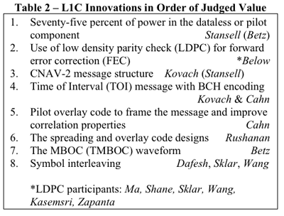
The L1C signal design is amazing, not only because of its highly evolved and outstanding technical performance but also because a committee designed this racehorse of a signal rather than it becoming a camel. Table 1 lists key members of the L1C technical committee in alphabetical order. The list has two groups, technical contributors and government chairpersons. When each new signal aspect is introduced, the key contributor or contributors from this list will be identified.
Table 1. Key L1C contributors.
L1C is intended to be interoperable with L1 signals from other GNSS providers. To identify its signal type, we note that Galileo officials have identified three types of services, “open”, “commercial”, and “publicly regulated”. An open service is freely available to all users. A commercial service is limited to users who pay a fee to access the signal, which otherwise is denied by encryption. A publicly regulated service (PRS) also is encrypted but intended only for public safety applications. GPS is adopting the open service definition but will continue to distinguish encrypted signals as “military” because there are no encrypted commercial GPS services. L1C will be a new GPS open service signal, joining L1 C/A, L2C, and L5.
Although the term “civil signal” often is used, there can be confusion about its meaning. Within the U.S. government it is common to use the word “civil” to mean civil government agencies, e.g., the Department of Transportation (DOT). However, it’s clear the GPS C/A, L2C, L5, and L1C signals are “open” and intended for use by anyone. Therefore, we will use the term “civilian” or “open” in order not to imply that any of these signals is restricted in its use.
L1C Signal Development
The L1C signal structure has evolved from the earliest GPS signals first launched in 1978. It shares with the C/A signal the L1 center frequency of 1575.42 MHz, coherence between the carrier frequency, the code clock rates, and the data rate, and the provision of a navigation data message. Significant improvements have been inherited from subsequent developments, specifically WAAS, L5, and L2C. For GPS or GPS-related signals, WAAS was the first to use forward error correction (FEC) for its data. L5 was the first open signal design to use longer spreading codes (10,230 chips), to have separate data and data-less (pilot carrier) signal components, to employ an improved navigation message structure (CNAV), and to employ overlay codes to achieve a longer equivalent code length, improve correlation performance, and eliminate the need for bit synchronization. The L2C signal adopted most of these improvements but, instead of an overlay, substituted a much longer pilot carrier spreading code, not only to optimize correlation performance but also to decrease the number of time ambiguities after tracking the spreading codes, i.e., extend the duration of GPS time ambiguity from 1 ms after tracking the C/A code and 20 ms after tracking the L5Q code to 1.5 sec for L2C.
Before giving details of the L1C signal in which we identify the primary contributor(s) for each innovation, it’s appropriate to recognize the special contributions of two members of the L1C technical team.
The first is Dr. Charles R. (Charlie) Cahn. Cahn has been a major contributor to GPS since before GPS was conceived. In particular, he was a key contributor to the Air Force 621B program which anticipated GPS. (He, Dr. James J. (Jim) Spilker, Dr. Robert Gold, and Mr. Burt Glazer deserve most of the credit for developing the original GPS C/A and P code signal structures, other than the NAV message.) Cahn discussed the merits of having a separate data-less or pilot channel in a 621B report [1], with Stansell he again recommended this for GPS in a 1975 Spartan Study Report, and finally the idea was adopted by the RTCA for L5 in accordance with recommendations from Cahn, Stansell, and Keegan. Also, Cahn was the first to recommend an overlay code on the L5 data signal to eliminate the need for the always problematic bit synchronization process. In a step toward L1C, Cahn was a primary contributor to the L2C design. In particular, he designed the code generators, including the 1.5 sec pilot code, and the chip by chip multiplexing technique which permitted two signal components in one bi-phase signal. In addition to consulting for The Aerospace Corporation and several commercial GPS companies, Cahn recently invented a more effective method to combine multiple signals on one carrier, called Phase-Optimized Constant-Envelope Transmission (POCET) modulation [2]. It is expected to be used on later versions of GPS III satellites to improve transmitter efficiency.
The second special recognition is for Dr. John Betz. Betz has played a very significant role for more than a decade in helping define the military M-code, in working with international partners to define and negotiate compatibility and interoperability signal parameters, in helping negotiate a significant part of the 2004 EU/US agreement, and in evaluating and supporting a wide variety of GPS programs and initiatives. Betz was a vital contributor to the overall L1C design through interaction with other team members, development of ways to compare alternatives, suggesting use of new signal processing concepts, and bringing experts from MITRE who performed significant analyses and developed key signal components.
Table 2 lists, in order of the authors’ judgment of value to user communities, the most important new characteristics of the L1C signal. The list also shows the primary contributor(s) for each characteristic.
Table 2. L1C Innovations in order of judged value.
Improvements made to the previously modernized civilian GPS signals, L5 and L2C, were a starting point for the L1C design. These included: having a pilot carrier; longer spreading codes (10,230 chips minimum); overlay or long pilot codes to eliminate the need for bit synchronization, to improve correlation properties, and to decrease the number of time ambiguities aft
er locking to the spreading codes; use of FEC to improve data demodulation performance and provide bit synchronization; and the flexible and higher precision CNAV message. The following paragraphs describe the additional improvements incorporated in L1C.
A key issue was whether additional signals could be added to the L1 carrier without negatively impacting legacy signals. Several combining methods were considered, and it was determined that, with the right combining technique, L1C could be added without detriment. Use of POCET, subsequently invented by Cahn, will further enhance this capability.
An “industry standard” rate ½ constraint length 7 convolutional coding method had been adopted for forward error correction (FEC) on WAAS, L2C, and L5 signals. However, the team agreed it was appropriate to consider other possibilities. Betz arranged for Ma to address the team on at least two occasions, providing a good tutorial on other advanced FEC methods which would allow message demodulation at even lower signal-to-noise ratios.
While the FEC options were being considered, another breakthrough occurred. Since at least 1999 Stansell had encouraged development of a way to take better advantage of GPS message redundancy. Rising to this challenge, Kovach proposed a modification of the CNAV message structure that he and Art Dorsey (Lockheed-Martin) had developed for L5 and L2C. The modified message, called CNAV-2, is equally flexible, equally precise, but more efficient, allows faster time to first fix (TTFF), and permits message demodulation at signals as weak as the carrier can be tracked. This final attribute requires FEC encoding of entire message blocks (sub-frames) rather than having the continuous process used for L2C and L5. As a result, when signal levels are very weak, bit symbols from two or more messages can be combined to improve the energy available per symbol, i.e., the L1C data demodulation threshold can be improved by combining symbols from two or more messages.
As a result of the message format improvements and performance evaluations by Shane, the team settled on the Low Density Parity Check (LDPC) FEC block encoding technique. This technique is as effective as turbo codes but without intellectual property constraints. Software developed by Shane was used by Sklar and Wang to define the specific L1C implementation, with performance simulation help from Kasemsri and Zapanta.
The most important new attribute of L1C resulted from a proposal by Betz to take advantage of the improved FEC and message redundancy attributes of L1C by having two separate data messages. Half the total signal power would be in the pilot carrier and the other half would be split evenly between two messages, one with full precision and the second with less precision but which could be acquired more quickly for faster TTFF. Stansell appreciated the opportunity for less power in the message but recommended that instead of having a second message the saved power should be added to the pilot carrier, for a 75/25 split between pilot and data power. The reasoning was that code and carrier measurements on the pilot are vital to navigation whereas messages are redundant, slowly changing, and are becoming available from other sources, such as the Internet and from cell phone networks. The issue was settled by an international survey of manufacturers, universities, and government organizations. The final L1C signal design, with the 75/25 power split, was selected by these experts from a group of five signal options.
Another L1C message innovation came about through a collaboration between Kovach and Cahn. The idea was to have a separate message sub-frame with very powerful encoding to identify GPS time of week to within a two hour interval. The sub-frame is called Time of Interval (TOI), and Cahn recommended a 52 symbol (26 bit) BCH code to provide the 9 bits of TOI information. Although orbit parameters may be available from a number of sources, precise and unambiguous time is vital for navigation, and TOI serves this and other purposes. With this level of encoding, TOI can be obtained from just one message at very low signal levels. Furthermore, the identical TOI is broadcast from every GPS satellite at the beginning of every 18 second L1C message. Therefore, it is possible to combine symbols from two or more GPS signals to demodulate TOI even under very adverse signal conditions. After locking to the pilot code and its overlay, one TOI establishes time of week within ±1 hour for all GPS signals.
TOI is particularly effective because of a recommendation by Cahn to overlay the pilot spreading code with another code which frames the entire data message. The L1C overlay code is 18 seconds long (the message length) and is unique to each GPS satellite. Because of this, the TOI defines which of the 400 possible 18 second intervals within a 2 hour time span begins at the next message frame, which also is the beginning of the next overlay code. If receiver time is known or can be determined to within an hour, TOI and the GPS spreading codes establish time for all GPS satellites.
Although it would have been adequate to adopt spreading codes from the L5 signal design, Betz introduced Rushanan to the L1C technical team and recommended that he study alternate code structures with improved characteristics. After an extensive study, Rushanan recommended a set of length-10223 Weil-codes extended with a fixed 7-bit pad to provide the primary L1C spreading codes. These codes have improved performance characteristics, as detailed in [3], [4], and [5]. In addition, the team asked Rushanan to define the 1800 chip pilot overlay codes, also described in [3], [4], and [5]. Stansell specifically requested that Rushanan optimize the ability to synchronize to the overlay code with as little observation time as possible. As a result, within one or two seconds after a signal is acquired, its 18-second time frame is established. After the first satellite is acquired, the maximum time difference for signals from other satellites is less than ±10 ms for receivers near the earth, so only two possible states of the overlay code must be examined to resolve the 18 second message phase for any other satellite. If the GPS almanac, an estimated position, and even a rough time estimate are available, as usually is the case, message time phase can be resolved even faster for subsequent signal acquisitions.
The L1C waveform originally was to have been a pure BOC(1,1) (a 1.023 MHz square wave modulated by a 1.023 MHz spreading code). Negotiations between the U.S. and the European Union (EU) at that time resulted in an agreement [6] that both GPS and Galileo would use a baseline BOC(1,1) signal. However, the EU reserved the right to further optimize their signal within certain bounds. Some of the optimization proposals were known as CBCS and CBCS. However, in further EU/US discussions it was decided that L1C and the Galileo E1 open service signal should have identically the same spectrum. This was a significant challenge because of different baseline signal structures and existing designs. The breakthrough came when Betz proposed what is called MBOC. The MBOC waveform has 10/11th of its power in BOC(1,1) and 1/11th in BOC(6,1). However, L1C and E1 OS achieve this result in very different ways. The Galileo technique is called CBOC, as described in a number of papers. [8], [9], and [10]. The GPS technique is called TMBOC and is defined by IS-GPS-800A [11] as well as by [3], [4], [5], and [8]. Whereas Galileo has a 50/50 power split between pilot and data and includes the BOC(6,1) component in each, GPS includes the BOC(6,1) waveform only in the pilot component by modulating four of every 33 spreading code chips with a 6 MHz square wave and 31 chips with a 1 MHz square wave. With 75% of the power in the pilot, the result is 3/4 x 4/33 or 1/11, as required. It is likely the BOC(6,1) signal component will be ignored by consumer grade GNSS receivers where a narrow RF bandwidth is preferred. Fortunately that is a loss of only 12% (0.56 dB) of the L1C pilot power. However, for commercial and professional grade receivers, the extra waveform transitions (wider Gabor bandwidth) can be used to improve code tracking signal-to-noise ratio, and with certain advanced techniques it should be possible to improve multipath mitigation. This final point depends on careful control or calibration of the transmitted code timing and symmetry.
Finally, Dafesh recommended that the team consider data symbol interleaving. The team accepted this suggestion, and Sklar and Wang designed the interleaver. Because of the powerful FEC, by scattering data symbols throughout sub-frames 2 and 3, it is possible to recover an entire message even if portions are blocked by, for example, walking or driving past trees or other obstructions.
All team members deserve credit for sharing, challenging, and improving concepts. Particular examples are the strong aviation navigation background provided by Hegarty and the in depth design experience for a wide range of receiver types and civilian applications provided by Keegan. In addition, Yi had the primary responsibility for documenting L1C in IS-GPS-800.
It also is important to recognize the contributions of the many professionals who responded to the worldwide survey of manufacturers, universities, and government experts. Stansell conducted each of the survey presentations, some in person and others over the Internet. One or more of the Government Chairpersons also participated, usually Hudnut or Lenahan. There were responses from organizations in 10 countries: Japan (34), the USA (26), Russia (7), the United Kingdom (5), Canada (4), Australia (1), Finland (1), Germany (1), Switzerland (1), and Taiwan (1). This is not a complete picture because a number of the responses were from individual experts while others were a consensus response from a larger group. Five signal design options were presented, and the preferred design received 62 percent of the 81 responses. As a result, the L1C signal has a 75/25 split between pilot and data power and the data rate is 50 bits per second.
L1C Signal Description
The official L1C signal description is given by IS-GPS-800; the most recent version A was released on June 8, 2010. Figures 1 and 2 show the L1C power spectral density with, respectively, a logarithmic (dBW/Hz) scale and a linear (Watts per Hz) scale. Figure 3 is the same as Figure 1 but also includes the C/A and M Code signals; it assumes both signals are transmitted with the same total power.
Figure 1.Figure 2.Figure 3.
These plots illustrate three important aspects of the L1C spectrum. First, L1C is designed to have only a small impact on reception of the legacy C/A signal. This is important for the compatibility of signals with respect to each other. A good way to evaluate the impact of one signal on another is called the Spectral Separation Coefficient (SSC), which quantifies the amount of interfering power from one signal to another, under the assumption that each signal is transmitted with the same power but with different spreading codes.
The SSC between a C/A signal and the L1C signal is –68.3 dB/Hz. The spectral separation illustrated in Figures 1, 2, and 3 assures that L1C signals will have very little impact on acquiring and tracking the legacy C/A signals. Therefore, L1C is judged to be compatible with the C/A signal.
Figure 3 also illustrates that L1C and the M Code signals have very little impact on each other. The SSC between L1C and M Code is –82.8 dB/Hz. This is important because M-Code power may be substantially higher than the civilian signals, so a larger negative SSC is important to maintaining compatibility.
The third aspect of the L1C spectrum is the additional signal power at ±6.138 MHz. This component of signal power differentiates a binary offset carrier BOC(1,1) waveform from the L1C multiplexed BOC or MBOC waveform. Exactly 1/11th of the L1C signal power is a BOC(6,1) component, whereas 9/11th of the power is a BOC(1,1) component.
75 Percent in the Pilot Carrier. Figure 4, which shows the required post-correlator C/N0 required to phase track either the L1C or C/A signals as a function of tracking loop bandwidth, illustrates the main advantages of having 75 percent of the L1C signal power in the pilot component. The carrier-tracking threshold for equivalent signal power using a Costas loop is 6 dB worse than tracking with a phase-locked loop (PLL). A Costas loop is needed for the C/A signal because it is modulated by data, whereas a PLL can be used for the dataless L1C pilot signal. This 6 dB advantage more than compensates for having only 75 percent (-1.25 dB) of the L1C power in the pilot. The vertical displacement between the two curves illustrates the 4.75 dB L1C tracking threshold advantage.
Figure 4. Required post Correlator C/N0 versus tracking loop bandwidth.
The horizontal displacement of the curves shows another L1C advantage. For a given C/N0 threshold, the L1C loop bandwidth can be increased by a factor of three. In turn, this allows tracking with G forces 32, or nine times higher. For third-order loops capable of tracking acceleration, this allows tracking with 27 times higher jerk. Such differences are likely to be more important than tracking threshold for high-dynamic applications such as machine control.
Although Figure 4 assumes the L1C and L1 C/A signals have the same total power, the minimum received L1C signal power specified in IS-GPS-800A is –157 dBW, and the equivalent for C/A in IS-GPS-200E is –158.5 dBW. In other words, the intent is for L1C to be transmitted with 1.5 dB more power than C/A. Therefore, the figure is conservative by 1.5 dB in evaluating the L1C advantages over C/A. Thus, the actual threshold advantage is 4.75 + 1.5 = 6.25 dB.
For narrowband or other receivers not punctual correlating the BOC(6,1) signal component, the pilot carrier is 29/33 or 0.56 dB weaker, so the net advantage is 4.75 – 0.56 + 1.5 = 5.69 dB.
LDPC Block Encoding
Low-density parity check (LDPC) encoding provides three key advantages. First, to demodulate the critical part of the L1C message with a bit error rate (BER) of 10-5 requires an Eb/N0 (ratio of energy per bit to the noise power in a 1-Hz bandwidth) of 2.2 dB versus 96 dB for the C/A signal. When taking into account that only 25 percent of L1C signal power is in the data component, the required total power of the L1C signal can be 1.4 dB less than the C/A signal for an equivalent BER. As a result, this performance allows the pilot component of L1C to have 75 percent of the total L1C power.
Second, LDPC gives near-optimum performance with no intellectual property constraints. Third is the ability to block-encode Subframes 2 and 3 of the L1C message, described next.
CNAV-2 Message. Figure 5 compares the L5 and L2C CNAV message structure to the L1C CNAV-2 structure. CNAV was a major step forward compared to the original NAV message in terms of flexibility, precision, time to first fix (TTFF), and integrity. Instead of the fixed 30-second structure of the NAV message, CNAV consists of multiple six-second messages that are differentiated by a message-type number. The sequence of broadcast message types is defined by the GPS control segment, which greatly improves flexibility. The round-off error in the NAV message can affect pseudorange calculations
by up to 40 centimeters, whereas the equivalent CNAV error contributes about 3 centimeters. Orbit and clock precision is substantially improved. Because a minimum of three message types are needed for the necessary orbit and clock parameters, as little as 18 seconds is needed to gather the necessary information after locking to a signal. On the other hand, if four message types are being sent sequentially, and the receiver locks just after the beginning of a message, it can take 30 seconds to gather the necessary data. TTFF typically is improved. Importantly, each CNAV message includes a 24-bit cyclic redundancy check (CRC) word that makes it practically impossible to have bit errors in a message that passes the CRC check.
Figure 5. CNAV and CNAV-2 message structures.
CNAV-2 improvements to the CNAV structure all but guarantee an 18-second TTFF after signal acquisition. Message efficiency is improved by eliminating the need to identify each six-second message, to have complete time-of-week (TOW) information in each six-second message, and to have three rather than two 24-bit CRC words every 18 seconds. Even more important, GPS time is defined modulo 18 seconds upon acquisition of only one signal, and it is defined modulo two hours by decoding only one 26-bit, 0.52-second time-of-interval (TOI) word at the beginning of each message. In addition, TOI is so well encoded (52 symbols for nine data bits) that it can be demodulated in very weak signal conditions, which can be further enhanced by combining the identical TOI symbols transmitted by every satellite at the beginning of every 18-second message.
Figure 6 illustrates the ability to combine message symbols from several sequential Subframe 2 data blocks so vital clock and ephemeris data can be demodulated at the weakest signal level the receiver can track. This feature is made possible because the symbols in subframe 2 will not change for at least 15 minutes (50 repeats) and typically no more often than one to two hours (200 to 400 repeats). This provides up to 8.4 dB of message demodulation improvement. The figure also shows other L1C improvements: 4.8 dB of carrier track threshold extension, and a TTFF of 18 seconds after successfully demodulating subframe 2 from the minimum number satellites for a position fix.
Subframe 3 of the L1C message contains less time-critical information such as almanac, ionospheric correction terms, and so on. This subframe also is LDPC block-encoded so it is quite robust, although it does not offer the ability to combine symbols from sequential messages.
Figure 6. L1C and C/A performance comparison.
Pilot Overlay Code
Figure 5 shows that the pilot overlay code consists of 1,800 chips that frame the 18-second message. In comparison with the L5 20-millisecond (ms) pilot overlay code, it not only is 900 times longer but also is unique to each satellite. This improves cross-correlation performance in general and particularly when two satellites have the same pseudorange.
The long L1C overlay code can be acquired reliably after only one or two seconds of signal lock. Its length does not cause a relevant delay in TTFF, but it provides many advantages. First, synchronizing to the overlay code on one satellite defines GPS time for all satellites modulo 18 seconds (in comparison to 1 ms with the C/A code). Even with infrequent use, the receiver’s RTC, which typically is better than 5 parts per million (ppm), should have sufficient accuracy — better than ± 9 seconds — to completely resolve GPS time with one signal acquisition. In 24 hours with a clock frequency error of 5 ppm the time drift would be less than ½ second.
Even if the RTC is in error by several times 18 seconds, resolving accurate time can be done quickly by computing position fixes with multiple time hypotheses spaced 18 seconds apart. Pseudorange changes at rates up to ±1,440 kilometers per 18 seconds. Because some satellites are approaching, others are moving away, and all of them are changing range at different speeds (different Doppler frequencies), determining which position fix is correct out of several 18-second GPS time hypotheses will be straightforward since only one will be reasonable. (Care must be taken to avoid any extremely rare instances where two results may seem reasonable.)
The worst clock error with aided GPS (A-GPS) is ±2 seconds, which is adequate to completely resolve GPS time after acquiring only one L1C signal. This capability can aid acquisition of and navigation with other signals, such as C/A or signals from other GNSS providers. The 18-second overlay code will provide benefits as soon as even a few L1C signals are available.
The L1C overlay code, in conjunction with the repeating symbols of message subframe 2, also enables data demodulation to begin at any point within an 18-second message. It is not necessary to wait for the message frame to begin. The receiver can begin collecting data symbols at any time, and 18 seconds later it will have assembled all the subframe 2 clock and ephemeris information and can begin to navigate. An exception occurs when the satellite message is updated, between once every 15 minutes to once every two hours. This capability significantly improves TTFF whenever satellite messages are needed for navigation, for example, when they aren’t still valid from a previous collection or aren’t provided by an A-GPS service.
Spreading and Overlay Code Designs
The L1C MBOC waveform (time-multiplexed BOC, or TMBOC), shown in Figure 7, enabled GPS and Galileo to have open-service L1 signals with an identical spectrum, although implemented quite differently. L1C places all the BOC(6,1) chips in the pilot carrier. This is because the BOC(6,1) component is intended to improve code-tracking performance by increasing code loop signal-to-noise ratio (SNR) and by allowing advanced multipath-mitigation techniques to have the advantage of more code transitions. Because these measurements are made almost exclusively on the three times (4.8 dB) more powerful pilot signal, there is no reason to lose the code tracking benefit by having BOC(6,1) chips in the data signal component. In addition, narrowband receivers such as those predominantly used for consumer applications cannot process BOC(6,1) chips, so it would be undesirable to deny full message signal power to such receivers.
Figure 7. The GPS MBOC (TMBOC) modulation.
For receivers tracking only the BOC(1,1) component of L1C MBOC, there are on average 43.5 code transitions per 33 chips. For those tracking both components, there are on average 89.5 code transitions per 33 chips. This provides up to 3.1 dB of improvement in code loop SNR for wideband receivers code tracking with both types of chips. (The amount of improvement depends on receiver RF bandwidth.)
Classic multipath-mitigation techniques such as the double-delta don’t work well with the BOC(6,1) waveform, but recent advances promise improvement by using the extra transitions in the MBOC signal. Some developers worry that the full benefit may not be achieved unless code symmetry and time alignment of the two components is better than the signal specification permits. If the satellites cannot provide the needed signal symmetry and alignment, such problems likely can be overcome by ground calibration of these characteristics, either directly by each receiver or indirectly by an observing network.
Symbol Interleaving. Symbol interleaving means that before a message is transmitted, the satellite scatters the 10-ms message data symbols from subframes 2 and 3 throughout these subframes in
a fixed and known pattern. After a receiver has demodulated (or otherwise measured) the symbols belonging in a subframe, they are reassembled into the proper order before the LDPC block decoding is performed. In other words, the scattering done in the satellite is undone by the receiver. The objective is to provide a measure of protection against certain types of signal fading. For example, if a sequence of symbols from the satellite is lost because the receiver passes behind an object such as a tree, only half the symbols in this part of the message would be affected if the adjacent symbols in the original message are received either before or after the signal blockage. Thus, with reasonable signal levels and the benefit of powerful LDPC block encoding, the entire message could be reconstructed.
Performance Metrics and Comparison
A main objective for the L1C signal structure was to significantly improve the autonomous navigation capability for GPS users. Key weaknesses in the current C/A signal include the thresholds for bit synchronization, message synchronization, and data-bit demodulation. To achieve navigation at very low signal levels, users of the L1 C/A signal had to employ external sources for time synchronization, data acquisition, and, to extend the tracking loop threshold, external data-bit aiding to enable phase-locked tracking rather than Costas tracking of the C/A signal. The new signal structure addresses all of these shortcomings and provides a robust autonomous navigation system that requires no external aiding for most commercial applications.
Message Frame Synchronization and Time of Transmission. For autonomous navigation, frame synchronization has two important roles. The first is to set GPS time, modulo frame duration, which is required to establish the unambiguous time of transmission. Frame synchronization, or knowledge of frame start, also enables assembly of the received bits into the appropriate data words. In both L1 C/A and L5, frame synchronization is accomplished by recognizing a synch word within a data subframe, which requires accurate demodulation of data bits. For L1C, frame synchronization is inherent in the signal structure and does not require demodulation of data bits. This is very important for two reasons. The first is to establish GPS time of transmission very quickly, especially when the satellite message is not needed, for example, if it was acquired previously or obtained by other means. The second is when satellite ephemeris data is necessary, but the signals are very weak. The L1C message structure facilitates this capability.
Overlay Code on Pilot Carrier. One frame of data consists of 1,800 symbols modulated onto the data carrier which, at 100 symbols per second, is 18 seconds long. However, synchronized to this 18-second data frame is a pseudorandom code modulated on the dataless pilot carrier. This 100 chips per second overlay code is a linear-shift-register code that is truncated to be 1,800 chips long. The overlay codes were chosen to have very low minor auto-correlation and cross-correlation peaks so a very short segment of the code can be used to establish its underlying code phase.
If a 100-chip segment of the received code is correlated over a replica of the entire code, the proper correlation peak would be easily distinguished, thus establishing the GPS time epoch at the start of the code. Since this code epoch and the start of the data frame are synchronized, the start of the entire data frame is established, modulo 18 seconds. The start of the data frame by definition establishes the GPS time of transmission, also modulo 18 seconds. This is accomplished without decoding a single data bit by using the power advantage of the pilot carrier.
However, using the message to resolve the 18-second time ambiguity often is not needed. For example, the receiver’s real time clock (RTC) is likely to be accurate to within ±9 seconds. Alternately, almost any source of external aiding can provide time to within ±2 seconds. In either case, if the receiver already has a valid satellite ephemeris, navigation can begin after receiving a little over 1 second of the stronger pilot carrier signal. Ephemeris data can be available in a number of ways, including prior reception from the satellite, from a separate communications channel, or from one of several predicted ephemeris sources.
Message Frame – Data Format. A message frame consists of 1,800 symbols that comprise two distinct data types. The first data type, in subframe 1, is the Time of the Frame (TOI or Time of Interval) modulo two hours. The second data type is further separated into two blocks, subframe 2 containing data that is fixed for a period of time and subframe 3 containing data that can change from frame to frame.
Time of Interval Subframe. The TOI is a count of the number of 18-second message intervals in each 2 hour time period. Two hours is the maximum duration of any ephemeris message before being replaced by the satellite. (Fifteen minutes is the minimum.) There are 400 18-second intervals in 2 hours, so it requires 9 bits to represent the 400 intervals. These nine bits are block-encoded into 52 symbols using a BCH(51,8) code, where the 8 data bits are the least significant bits of the TOI. The most significant bit (MSB) of the TOI is then mod-2 added to the BCH codeword and also appended to the resulting codeword as its MSB, resulting in a 52-symbol codeword. This coding provides a BER of 10-5 for an Eb/N0 of –1.9 dB per coded symbol or a C/N0 of +18.2 dB-Hz at the correlator output for the data channel. Since the data channel contains only 25 percent of the total L1C power, the C/N0 of the composite signal would be +24.2 dB Hz. Symbol demodulation is performed using the pilot carrier tracked by a PLL as the phase reference. Since the pilot carrier contains 75 percent of the total power, its C/N0 would be +23 dB-Hz. With a (single-sided) loop-noise bandwidth of 10 Hz, the loop SNR for the carrier channel PLL would be +10 dB.
Note that a 10-5 BER is not required for successful demodulation of TOI. Therefore, weaker signals can be used successfully if the PLL loop bandwidth can be smaller in such weak signal conditions.
The most straightforward method to decode the TOI is brute force maximum likelihood estimation. All possible code words for the 400 possible data words can be pre-computed. Each then can be compared (correlated) with the received code word. The data word that corresponds to the code word with the highest correlation would be the result of the decoding process.
Finally, since all satellites simultaneously transmit the same TOI, the received code word from several satellites can be combined to increase the effective Eb/N0. The target BER of 10-5 thus can be achieved at an even a lower C/N0 than the single satellite value. In this case, the decoding process described above can be performed on a composite code word derived from two or more satellite signals, weighted appropriately for the signal strength from each one.
As an example, consider a receiver with access to an external source of the ephemerides. By combining the TOI code word from five satellites, the average C/N0 required per satellite would only be 17.2 dB-Hz, so time could be established to ±1 hour in slightly over 1 second.
Because of the 18-second overlay code, decoding TOI is not required for receivers with an internal clock good to ±9 seconds or with external time aiding, the worst of which today is within ±2 seconds.
Data Subframes. The remaining data bits are separated into two additional subframes. (TOI is in the first subframe.) The second subframe contains data that does not change for at least 15 minutes, and typically for an hour or two. This subframe provides the satellite ephemeris and the interval time-of-week (ITOW) count, which identifies the start time of the two-hour interval since the beginning of the GPS week, which, in turn, frames the TOI count of 18-second intervals within each two-hour frame. The third subframe contains data that normally changes from frame to frame, such as the satellite constellation almanac.
The block of data containing the satellite ephemeris (subframe-2) consists of 576 clock and ephemeris bits along with a 24-bit CRC, for a total of 600 bits. These are encoded with a rate-½ LDPC Block code into 1,200 symbols. The block of data containing variable data (subframe-3) consists of 250 data bits along with a 24-bit CRC, for a total of 274 bits. These are also encoded with a rate-½ LDPC Block code into 548 symbols. The 1,748 symbols of the two data subframes are combined and interleaved using a simple 38 x 46 row-column block interleaver. These interleaved symbols plus the 53 TOI symbols make up the entire 1,800-symbol (900-bit) message frame.
Since both the LDPC codes and the interleaver operate on independent blocks of data, the resulting symbols for subframe-2 are identical and in the same location in each message frame for between 15 minutes and two hours. Since the data decoding uses the pilot carrier as the phase reference, the subframe-2 symbols can be coherently combined over many 18-second message frames before decoding to improve BER performance.
One reasonable subframe-2 strategy would be to check the CRC after LDPC-decoding the first received message to determine if there are any remaining bit errors. If errors are detected, do the same with the second message. If errors exist in the second message, coherently combine the symbols from the two messages, properly weighted, LDPC-decode the combination, and check the resulting CRC for errors. If necessary, this process can be used on as many messages as needed to obtain a perfect result.
Framing the data messages with the pilot overlay code and the repeating characteristic of subframe 2 permits data collection over any arbitrary 18-second interval. It doesn’t matter where data collection begins. The overlay code tells the receiver which symbol is which, and the repeating subframe-2 message can be compiled from any place in the previous message to the same place in the following message. The powerful CRC assures that a good message is perfect. When the ephemeris is needed from a satellite, rather than from an alternate source, these characteristics allow TTFF to be slightly over 18 seconds, with assurance the information is correct.
Since LDPC FEC has been adopted by the current state-of-the-art wireless standards such as 802.11n and 802.16e, employing it in the latest GPS signal structure should be simple for the receiver designer. In fact, synthesizable cores are available for WiMax LDPC decoders from several sources, and LDPC decoders are as commonplace in wireless signal basebands as Viterbi decoders for the convolutional codes of L2C, L5, and SBAS have become in GPS basebands.
For subframe-2 data, the Eb/N0 required to achieve a BER of 10-5 is approximately 2.2 dB. For subframe-3 data, the Eb/N0 required for this same performance is approximately 2.7dB.
Signal Structure
The L1C signal is a composite of two signals that are phase/frequency coherent with synchronized spreading codes and symbol timing. The pilot signal has 75 percent of the total power, is a carrier-only signal, and is spread by a 10-ms long code plus an 18-second overlay code. The data signal has 25 percent of the total power, is spread by a 10-ms long code, and is data modulated with 10-ms symbols.
Spreading Codes. The spreading code for both L1C signals are 10,230 chip codes with a chip rate of 1.023 MHz, producing a 10-ms long code. This corresponds to one symbol for the data carrier and one chip of the overlay code for the pilot carrier. These codes are not linear shift register sequences like all other codes employed by GPS, but are pseudo-random sequences derived from Weil sequences of length 10223. This sequence is extended by a 7-bit sequence 0110100, which is the same for all satellites, to the required length of 10230. The location within the particular Weil sequence where the extension sequence is inserted is called the insertion index. A pair of Weil indices and a corresponding pair of insertions points then determines the pair of codes for each satellite.
Synchronization to one of these Weil-based codes can be accomplished with a standard time-domain correlator, but the number of potential hypotheses has increased by a factor of ten compared to the C/A signal. However, this is no different than time-domain correlation for an L5 code, which also are 10,230 chips long. Synchronization also can be accomplished using FFT-based frequency-domain correlation, however it does require an FFT of length 65,536 (for a standard radix-2 implementation) since the FFT must span 2 full code periods at a minimum of 2 samples per code chip (40,920).
To compare L1C frequency domain correlation with L1 C/A, a frequency search window and integration time must be hypothesized. A simple example would be a 10-ms coherent integration time and ±250 Hz frequency uncertainty. Table 3 compares the number of complex operations required for L1 C/A vs. L1C.
Table 3. Comparison of FFT-based correlation for L1C versus L1 C/A. (Click to enlarge.)
For cases where large search window uncertainties exist, and frequency domain correlation provides a computational benefit, an alternate approach to L1C synchronization would be to first obtain L1 C/A synchronization using an FFT-based search, providing frequency and 10 timing hypotheses (perhaps more with potential cross-correlations for L1 C/A). These L1C hypotheses could be tested by simple time-domain correlation that would benefit from the much better cross-correlation properties of the L1C codes.
For cases where time uncertainty is not large, a time domain search of the L1C code would be no more difficult than the equivalent for L1 C/A. For cases where the time uncertainty is small but the frequency uncertainty is large, time-domain partial-period correlations could be combined in an FFT structure that would span a large frequency uncertainty with a single time hypothesis. For example, the 10,230 chips could be separated into 62 segments, each 165 chips long. The 62 segments could then be combined using a zero filled 64-pt FFT to produce 64 full correlations spanning ±3 kHz.
MBOC Waveform. The L1C spreading code is further modulated with a code clock synchronized 1.023 MHz square wave creating the BOC(1,1) signal that forms the majority of the L1C code symbols. This produces a code that appears as a 1 MHz square wave, synchronized to the Weil-based code edge, whose polarity indicates the state of the Weil-based code chip. This BOC(1,1) sequence modulates all of the data channel chips and 29 of every 33 pilot channel chips. The other 4 out of 33 Pilot channel chips are modulated by a BOC(6,1) code symbol in which a 6 MHz square wave is used instead of the 1 MHz square wave for the BOC(1,1) chips. (Recall that ‘1’ signifies 1.023 MHz and ‘6’ signifies 6.138 MHz.) For receiver designers who choose not to punctual correlate the BOC(6,1) component of the pilot carrier, the pilot carrier power will be reduced by ~0.6 dB.
The BOC(6,1) signal component provides an opportunity for better performance of advanced multipath mitigation techniques. The presence of multipath interference not only impacts the code-tracking process of a GPS receiver but also distorts the waveform seen by the phase-tracking process of the receiver. The distortion of the phase of the received signal is most problematic when the reflector creating the multipath signal is very close to the receiving antenna, because the path length of such a multipath signal changes very slowly. Since the path length changes very slowly, it appears as an almost constant bias error in the phase measurements. The only way to observe this distortion, and hence measure its impact on the phase measurements, is to observe the phase of the carrier very close to the code transitions. The estimate of this distortion obviously is better the more frequently it can be observed. This is particularly important because the distortion is not constant but slowly changes. The MBOC signal combination provides
just over twice the number of transitions at which to observe the phase distortion than the BOC(1,1) signal alone, which is important for higher fidelity measurements during short intervals when the slowly changing distortion is highly correlated .
L1C Status
Companies already are designing L1C into their new chipsets, even though the first satellite to carry the signal is not expected before 2014. When will L1C be available from enough satellites to be meaningful? Figure 8 is a guesstimate of how modernized GPS signals will become available over the next decade. The projections assume either two or three successful satellite launches per year, and many observers think two per year may be realistic. Because GPS only launches on need to sustain the constellation, the actual launch rate depends on the lifetime of the satellites now in orbit. The first launch of a GPS III may be delayed until all IIF satellites have been launched, or the first GPS III, if available, may be launched before the last IIF to test the new design in space as soon as possible.
Some L1C signal and message characteristics will significantly benefit users of C/A and other GNSS signals by, for example, quickly resolving time for all GNSS signals. Therefore, L1C will provide meaningful benefit as soon as even one signal can be tracked from any location on earth. That might be possible with as few as six GPS III satellites in orbit, depending on where in the constellation they are deployed.
Figure 8. Guesstimate of modernized GPS signal availability.
Tom Stansell heads Stansell Consulting, after eight years with the Johns Hopkins Applied Physics Laboratory, 25 years with Magnavox (staff VP), and five years with Leica Geosystems (VP), pioneering Transit and GPS navigation and survey products. He led technical development of the GPS L2C signal and coordinated the GPS L1C project (2004–2006). He is a member of the Editorial Advisory Board of GPS World.
Ken Hudnut applies new technologies such as GPS to earthquake research as a geophysicist for the U. S. Geological Survey in Pasadena, California. He served as project manager for the GPS L1C signal design project from 2003. He received his Ph.D. from Columbia University.
Rich Keegan has 36 years of experience in radio navigation including Transit, Timation, Omega, Loran C, as well as GPS for the past 28 years. He has been the principal of a consultancy in digital communications and navigation since 2000. He was a member of the L2C and L1C modernization committees.
Early morning on February 2, 2011, I went to work in my job as a road surveyor in the Bungoma District of Kenya. Here, land disputes are common, though the government is trying to reduce the conflicts by issuing land titles and certificates.
I carried with me a small handheld GPS, the Magellan Explorist 100. While I was using it, a stout man in early fifties approached me and introduced himself as a surveyor, too. He was very interested in the way I was walking around with the “gadget,” trying to locate a control point. He asked me how the gadget worked. I explained it to him, showing him how its easy to use in general boundary surveys. He was satisfied, and we exchanged contacts and parted.
A month later, he called me for help. When I asked him what was wrong, he told me there were a group of land owners, or members, who were about to kill each other in a dispute over a 128-acre farm they had bought. These members had each contributed money to buy a single parcel with the intention of subdividing it fairly. They were engaged in a disagreement about the boundaries and the subdivision of the farm. The gentleman asked me if I could take a survey of the farm sometime in the next few days. Concerned about the conflict, I answered, “Yes, in hours not days.” Still, it wasn’t until two days later that he could assemble the members of the disputed farm and called me to mark the boundaries for them.
I arrived at the farm with my Magellan GPS and my laptop. To my dismay, I found that some of the members were armed with crude weapons, ready to fight each other. I asked them to be peaceful and wait for just a few hours while I surveyed the site.
I started picking the boundary corners of the farm all around the permiter. I was through with that task in less than 35 minutes. This parcel of land was to be divided into 18 pieces. I uploaded the data manually to my laptop, then I did the subdivision using AutoCAD Land Development 2000.
After two hours and fifteen minutes, I called the members and told them to ready themselves to be shown the boundaries of their property.
I walked around the property with them, guided by my handheld GPS, to each boundary beacon. After one and a half hours, the warring members were shaking hands and laughing, saying “So, it was that easy!”
The dispute had ended, and was solved peacefully. My small Magellan Explorist 100 acted as a peace mediator.
Noah Kertich is a surveyor with H Young Construction EA Ltd., which is under contract with the World Bank in conjunction with the government of Kenya. Kertich graduated from the Kenya Institute of Surveying and Mapping in 2004 and received a diploma in photogrammetry and GIS from Icaros Geosystems, Israel, in 2008.
Yesterday I conducted a webinar titled “A Closer Look at L5: The Future of High-Precision GNSS.” Preparing for it was quite interesting, so I thought I’d share some of the slides I produced (and had produced) for the webinar. I think you’ll find them interesting.
The webinar was focused on discussing the value of the new L5 civilan frequency for GPS/GNSS receivers. An interesting challenge in preparing for the webinar was my attempt at estimating what a satellite constellation of satellites (GPS and others) broadcasting at least L1 and L5 would look like four or five years from now. The point of it was to illustrate that a useful constellation of satellites broadcasting L1 and L5 (as well as L2C) is potentially only four to five years away.
In that timeframe, there are potentially 30 satellites that would be healthy and broadcasting navigation signals on the L1 and L5 frequencies that we can use. How is that possible?
Both GPS and Europe’s Galileo support the new L5 civil frequency (as well as L1). The U.S. has already launched one of the new GPS model IIF satellites. The IIF is currently healthy and broadcasting three civil frequencies; L1 C/A, L2C and L5. There are 11 more of the IIF satellites being built. It’s estimated that all 11 will have been launched into their orbits by ~2015. On the other hand, the first 18 Galileo satellites have been contracted to be built, and it’s estimated that the 18 will be launched into their orbits by ~2015. The Galileo satellites are designed to support L1 and L5 (as well as others). That’s a total of 30 satellites broadcasting L1 and L5.
In an ideal world and in the best interest of the civilian user community, the Americans and Europeans would coordinate orbits planes/slots of the 30 satellites so they would be in an optimal configuration (steady # of visible satellites, reasonable PDOP) for the user community. But, I seriously doubt that’s going to happen.
So, the next best thing is to attempt to estimate what an “uncoordinated” constellation of 30 GPS/Galileo satellites would look like in 2015 (assuming the launch schedules hold). Fortunately, our friends at the Galileo Supervisory Authority (GSA) have already mapped out the orbit plane/slot data for the 18 satellites. Without that data, none of these projections would have been possible.
GPS was a little tougher to estimate. The U.S. Air Force doesn’t have (or at least they don’t share) a long-range plan for where the next 11 IIF satellites are going to be inserted in the GPS constellation. They look out one satellite at a time. That’s understandable because the health of the GPS constellation changes over time. However, the U.S. Air Force does present a “watch list” of the weaker satellites in the constellation so we have some idea of where the new ones are going to be placed.
Once we compiled the information from the Galileo folks and our projections on where the next 11 IIF GPS satellites will be inserted, we were able to come up with some interesting plots I’d like to share with you.
All of the following satellite visibility plots are based on my location in Portland, Oregon, USA, and with a 15º elevation mask. Using a 15º elevation mask is pretty conservative so the plots are pretty conservative if you’re working in an open-sky environment like in agriculture.
The first plot is of the 12 GPS IIF satellites only. You can see there’s an average of about three IIF satellites in view between 6 a.m. and 8 p.m. Thanks to Analytical Graphics, Inc. for help generate the following plots.
The next plot is of the 18 Galileo satellites. You can see there’s an average of 4-5 Galileo satellites in view between 6 a.m. and 8 p.m.
The next plot is of both the 12 GPS IIF satellites and the 18 Galileo satellites. You can see there’s an average of 8 GPS IIF and Galileo satellites in view between 6 a.m. and 8 p.m.
Finally, the last plot is of the 12 GPS IIF satellites, 18 Galileo satellites, and the 19 remaining legacy GPS satellites (broadcasting L1 and L2). You can see there’s an average of 12 GPS IIF, Galileo, and legacy GPS satellites in view between 6 a.m. and 8 p.m.
For a different perspective, here are 3D orbit plots of the 18 Galileo satellites and the 12 GPS IIF satellites.
3D orbit plot of 18 Galileo satellites
3D orbit plot of 12 GPS IIF satellites
There are several more plots similar to these in my webinar for different locations around the world including London, Rio de Janeiro, New Dehli, Perth, and Bangkok. In the webinar presentation, I also provide more details about the benefits of L5. You can view a recording of the webinar by registering here. After registering, you’ll receive an e-mail with instructions on how to view the webinar.
Trimble today announced that it has entered into a definitive agreement to acquire certain assets related to the OmniSTAR GNSS signal corrections business from Fugro N.V. The acquisition is expected to significantly expand Trimble’s worldwide ability to provide corrections services for land based agriculture, construction, mapping, and geographic information system (GIS) and survey applications.
Trimble and Fugro also entered into a multi-year service agreement which includes Fugro’s ongoing operation of its correction network and satellite service broadcast systems that power the OmniSTAR service. Fugro’s offshore marine business is unaffected. Closing of the transaction, anticipated in the first quarter, is subject to certain closing conditions. Financial terms were not disclosed.
OmniSTAR provides space-based GNSS correction services that can improve the accuracy of a GNSS receiver for precise positioning applications. These are the four levels of OmniSTAR service:
VBS offers sub-meter positioning.
XP service delivers better than 20-centimeter accuracy.
HP service delivers greater than 10-centimeter accuracy.
The new OmniSTAR G2 service combines GPS-plus-GLONASS-based corrections to provide decimeter level positioning.
Trimble pioneered RTK technology in the early 1990s, which enabled high-accuracy corrections for field applications. RTK is now recognized as the industry leading technology for centimeter-level positioning. To further improve accuracy, Trimble subsequently introduced VRS technology in 2000 and shortly after that Trimble VRS Now Service.
“With the addition of the OmniSTAR services and our strong relationship with Fugro, we will offer a full range of high-precision positioning capabilities which now includes satellite-delivered corrections,” said Patricia Boothe, general manager of Trimble’s newly-formed Positioning Services Division. “Today, our agriculture customers use OmniSTAR services to perform planting, harvesting, variable rate application and many other operations. Our expanded portfolio will provide not only farmers, but also surveying, construction, and GIS professionals with more options to satisfy their particular accuracy, delivery, and financial needs.”
“Trimble and OmniSTAR have enjoyed a long standing relationship,” said John Waits, president of OmniSTAR. “The transfer of land-based GNSS signal corrections assets marks the next phase of our efforts to bring a broader range of positioning services to our combined customer base, on land and offshore. The OmniSTAR and Fugro teams remain committed to providing industry leading corrections services for customers who own a variety of GNSS receivers.”
The OmniSTAR business will be reported as part of Trimble’s Engineering and Construction segment.
Spectracom, a global provider of time and frequency test and measurement solutions, will make available its new 16-channel GPS constellation simulator, the Pendulum GSG-55, in March. The GSG-55 is the latest in the Pendulum line of GPS receiver test instruments and part of its solution set for receiving, distributing, and validating GNSS systems.
With the enhanced signal generating capability of the GSG-55, it is possible to simulate Satellite-Based Augmentation Systems (SBAS), the company said. Navigation systems that use SBAS can improve the accuracy and reliability provided by the GPS satellite signals alone, enabling critical applications such as aircraft navigation, and surveying and mapping. SBAS simulation (support for Europe’s EGNOS and North America’s WAAS) is a new feature in the GSG-55. It is also able to generate white noise, making it possible to test receiver sensitivity under different signal-to-noise ratios.
“Many high-end GPS applications utilize 12-channel GPS receivers. Our new GSG-55 GPS constellation simulator can fully test those receivers with additional signals for more comprehensive testing in both development and production environments,” says Staffan Johansson, product manager at Spectracom.
The GSG-55 builds on the popular Pendulum GSG-54 eight-channel simulator including accurate testing of GPS timing receivers and portability through its compact and lightweight bench-top chassis. The GSG-55 also continues the Pendulum brand hallmark of ease-of-use. As such, the entire GSG family of GPS simulators has been improved based on customer feedbac, the company said.
The presence of different types of devices, spanning multiple GNSS receiver types, configurations, hardware, software, and consequent widely varying capabilites, among a user mix of vehicles, cyclists, and pedestrians, poses several engineering challenges for a V2X scheme in which all road users share data with each other and with the road infrastructure.
The use of location awareness for transportation safety, efficiency, and security — a major area of research and development for academics, automotive manufacturers, and organizations such as the U.S. Department of Transportation — has focused attention on enabling communication between vehicles and other road user entities in a concept know as V2X, a term encompassing both vehicle-to-vehicle (V2V) and vehicle-to-infrastructure (V2I) systems, so that they can share location and other status information. As a result, any road user entity may see all others around it. This capability is almost always built on GNSS technology.
Future V2X systems will be able to include all road user entities, ranging from vehicles to cyclists to pedestrians, in this information-sharing system. While it sounds natural for everyone to talk to each other and share data for collective benefit, the presence of different types of devices among this user mix poses several engineering challenges. As an example, a V2X device in a vehicle may have a built-in GNSS receiver with a roof-mounted antenna and another vehicle may have a retrofitted V2X device with a passive antenna and relatively limited accuracy capabilities. As the GNSS technology further develops, some vehicles may have multiple-frequency GNSS capability compared to legacy single-frequency devices. In essence, all compatible V2X devices will have to be carefully designed to ensure their interoperability with the rest of the system.
This article investigates positioning challenges arising from multiple GNSS receiver types, configurations, hardware, and software in a V2X operational environment. This produces a clear need to have minimum performance standards for V2X-capable GNSS receivers. The article further investigates the implications of land-based visibility obstructions on relative positioning, and implications on standalone position accuracy both as a result of limited GNSS satellite visibility and WAAS satellite visibility.
V2X Background
V2X systems rely on two critical enabling technologies: communications and positioning. Organizations and industry collaborations have developed and demonstrated various V2X systems over the last few years. These efforts have produced interoperable prototype V2V and V2I systems and over-the-air (OTA) messaging standards.
Figure 1 illustrates the general concept of combined V2V and V2I, or V2X. In a fully operational system, all vehicles and other road users carry short-range communication and positioning technology. At present, these technologies are expected to be based on dedicated short-range communication (DSRC) and GNSS, respectively. This enables each user to be location-aware and capable of sharing their location with others. Vehicles may use built-in systems, retrofitted devices, or those based on the occupant’s personal mobile device. Infrastructure elements and other road users such as pedestrians also form part of the V2X user community.
V2X Relative Positioning. Relative positioning of all communicating entities with respect to a given user is a required functional capability of a V2X system. To enable this functionality, positioning information from all communicating entities must be exchanged. For automotive V2X applications, Society of Automotive Engineers (SAE) J2735 DSRC Message Set Dictionary serves as the primary standard for message definitions. Current version of the messages consists of a basic safety message (BSM) , an optional variable rate message (VRM), and an option for including proprietary messages.
With BSM and VRM, vehicle position, speed, heading, and GNSS measurements can be communicated to others. GNSS relative positioning techniques such as real-time kinematic (RTK), code-based differential, or individual position differing (that is, distance between the positions reported by individual vehicles) can be used for relative positioning. The latter method, also known as DPOS, is a particular focus of this article.
Given the above, a system developer may develop a V2X relative positioning system that can operate based on techniques that can be broadly classified as position-based techniques, which include DPOS, and measurement-based differential techniques, including RTK and others.
The Simpler Approach. The SAE J2735 BSM accommodates the simpler approach of using the DPOS method, as it enables the sharing of critical state parameters. This approach is very attractive as it requires minimal OTA data volume compared to sending GNSS measurements. Secondly, DPOS relative position estimation process requires only a fraction of the processing resources required compared to measurement-based differential processing. Thirdly, any GNSS receiver in the market today is capable of outputting a position solution and most of the critical GNSS state parameters required for the V2X BSM. In contrast, most low-cost devices do not output measurements required for other methods.
However, there are quite a few challenges associated with DPOS. A vehicle or any other road-user entity, such as a location-enabled handheld device, will share its location information via BSM only. A relative positioning engine in each entity will use this information to provide lane-level and road-level data (relative distance, speed, and orientation) for its V2X applications. The challenges associated with DPOS method arise from multiple stages in this process.
The presence of many road-user types brings in the possibility of thousands of GNSS receiver types, models, hardware, and software in the user group. Thus the system must be interoperable with devices with a wide range of performance characteristics.
Secondly, each entity will transmit BSM only. This OTA information offers no information about the constellation the GNSS device sees or how the solution was derived in terms of filtering or applied constraints.
Thirdly, the position accuracy reported by each entity is a GNSS device-dependent variable, an estimate of the actual error as derived by a user device.
Finally and most importantly, V2X applications expect relative positioning information for each communicating entity classified in one of three possible accuracy categories: Which Road, Which Lane, or Where-in-Lane (see “Is GNSS up to the V2X Challenge?” GPS World, October 2010). The V2X system must be able to reliably identify this accuracy classification for each communicating entity with the limited information provided via the BSM.
Study Goals. To illustrate the impact of these challenges, several GNSS receiver types, configurations, and operational scenarios were investigated.
Between multiple receiver types: In a V2X environment, vehicles and other road user entities may have different GNSS receiver types and makes: dual-frequency, single-frequency, and so on.
Same receivers using different parts of visible constellation: In an urban canyon, it is possible for two adjacent vehicles to see two different parts of the GNSS constellation, due to obstructions.
WAAS-enabled and non-WAAS receivers.
Data Collection
This data is a combination of field-data collections and a series of RF record playbacks. The field vehicle-mounted test setup included two GPS receivers, a GNSS L1 RF data recording device, and a high quality GPS/INS reference system (Figure 2). Type A receiver is a hi
gh-sensitivity enabled, automotive-grade GPS L1 receiver using a patch antenna, WAAS-capable although WAAS usage was disabled in the real-time data collection. Type B receiver is a high-quality L1/L2 receiver using a geodetic-grade antenna, used with WAAS enabled. The GPS/INS system was connected to the geodetic-grade antenna. The RF recording system was also connected to the automotive-grade GPS L1 antenna.
Figure 2. Vehicle test set-up.
The data was collected on a test route in Detroit, Michigan, that included durations of urban and deep urban canyon (40 miles per hour (mph) or less), freeway (55–70 mph), and suburban/local (30 mph) driving.
The RF data were subsequently replayed to GNSS receivers that were not a part of the field set-up. RF data was also replayed to receivers with forced sky-visibility obstructions and various WAAS settings. For limited sky-visibility tests, certain satellites were removed from each receiver’s view by receiver-specific configuration software. The satellite selection and restriction was done to mimic typical sky-view obstructions encountered in normal driving.
Type A receiver was chosen to illustrate the impact of visibility differences. A total of 13 satellites were visible in the entire data set (Figure 3). To create obstructed sky-view scenarios, two Type A receivers were configured to not use certain satellites in their position solutions. These configurations were:
Configuration 1 (C1): PRNs 7, 10, and 13 blocked
Configuration 2 (C2): PRNs 6, 16, 21, and 31 blocked
C1 mimics a vehicle/receiver with no visibility in the Northwestern part of the sky, whereas C2 mimics a receiver without visibility in the East/Northeastern part of the sky. Sky visibility restrictions do not vary with the heading changes of the vehicle. For example, for C1 receiver, Northwestern sky is always obstructed regardless of the vehicle orientation.
Figure 3. Sky view during the test.
Figure 4 shows an example RF data replay setup. The record and replay system was controlled through a PC and the recorded data was also stored in the controller PC. The output RF signal was split into multiple outputs such that multiple receivers can be tested at the same time. For each replay of the RF data, a benchmark receiver was also used to verify that there is no run-to-run difference as a result of the RF replay.
Outputs from each GPS receiver from field and replay runs were logged to PCs using receiver specific binary formats. The recorded output from each receiver included its position, position error estimate, velocity, satellite-specific measurements and indicators such as pseudorange, carrier phase, and signals-to-noise ratio.
Figure 4. RF data replay set-up.
Data Processing and Analysis
The data was first decoded from the receiver-specific formats to a common format, then corrected for antenna offsets. To simplify the process, the reference system position solution was translated to the position of the test antenna using the known between-antenna distance and orientation of the vehicle as measured by the reference system. As a result, all the receivers and the reference system are reporting the location of the test antenna. Then, data fields such as position and velocity for each receiver were time-matched with the reference solutions, and the actual error was calculated.
For a limited dataset, additional measurement-level differential processing was done to show the difference between a DPOS and an RTK or a code-based differential relative position solution.
Figure 5 shows a plot of the 2D position error observed from each receiver during the test as a function of driving environment. Overall, Type B receiver shows better accuracy as expected from a dual frequency high quality receiver. However, it shows spikes of large error increases at times, mostly observed in the freeway scenario with large error excursions. With Type A receivers, relatively larger errors are observed with the limited-constellation receivers.
Figure 5. Position error (2D) of each receiver as a function of driving environment.
Figure 6 shows the number of satellites used by each receiver in the same environments as in Figure 5. Overall, Type A receiver tracks and uses on average 2–3 satellites more compared to the Type B receiver, likely due to its high-sensitivity capability. Type A C1 and C2 receivers also track and use 2–3 satellites fewer compared to the all-in-view Type A receiver.
Figure 6. GPS satellites used by receivers.
Freeway Data. The vehicle heading in this segment was predominantly north or northwest. The sky view can be considered a combination of urban and open sky conditions. As highlighted in Figure 6, all-in-view Type A receiver was able to use up to 11 GPS satellites with an average of around 9 satellites. Type A C1 and C2 receivers used, on average, about 3 satellites fewer than the all-in-view receiver. All three receivers show satellite count drops down to 4 at certain times in this segment.
The satellite count of the Type B receiver shows the limitations of not using the high-sensitive tracking capability. The satellite count shows frequent drops below 4 satellites and on occasion down to no satellites used.
Although the satellite count difference between all-in-view Type A and C1/C2 receivers was forced by means of receiver configuration, short-term sky visibility restrictions that resemble these conditions are in fact possible. Examples include a passenger car driving next to a semi truck or the side wall of the freeway in below-ground road sections.
Figure 7 shows the position outputs of all four receivers on a satellite image of a short segment of the freeway. The true location (reference) is shown in green. Type A, Type B, Type A C1, and Type A C2 are shown in red, black, purple, and blue, respectively. These colors identify the four receiver types in all figures for the rest of this paper. While biases can be seen in the outputs of all four receivers with respect to the reference, the Type A C1 shows the largest offset with the magnitude of more than a lane width.
Figure 7. Freeway positioning accuracy.
Figure 8 illustrates a time series of the positioning error components of all four receivers. It clearly shows error ramp-ups from the Type B receiver at frequent intervals. These coincide with the satellite count drops of Type B shown in Figure 6. No such error ramp-ups are observed for any of the Type A receivers, although relatively large biases of the order of few meters can be seen. As anticipated, larger errors are observed in the height direction.
Figure 8. Freeway positioning accuracy time series.
Local Road, Eastbound. This segment includes data gathered on an eastbound multi-lane local road with 40 mph posted speeds. As shown in Figure 6, a relatively larger number of satellites were continuously tracked in this segment as compared to the freeway. Therefore, this segment is considered to be an open-sky scenario with very limited number of obstructions. As shown in Figure 6, Type B receiver has used about 6 satellites on average, whereas the Type A has used around 3 more satellites most of the time. Type A C1 and C2 have also used around 3 satellites less compared to the all-in-view Type A receiver.
Figure 9 shows the vehicle position as reported by all three receivers and the reference system output for a short road segment in this drive. It clearly illustrates the lateral offsets of both C1 and C2 solutions. The C2 receiver (Blue) generated about a lane width offset towards north whereas the C1 receiver output is biased by around two lane widths to the south. Figure 10 presents a time series look of the positioning biases evident in Figure 9. It clearly shows large (more than 5 meter) biases in North and East position error components for C1 and C2 receivers.
Figure 9. Local (east) positioning accuracy.Figure 10. Local (east) positioning accuracy time series.
Local Road, Northbound. In roadway characteristics, this resembles Local Eastbound. Figure 6 shows the sky view remained almost unchanged for Type A receivers. For Type A C1, the count remained at 6 throughout. C1 and C2 receivers tracked 2–3 satellites fewer compared to all-in-view Type A. Interestingly, Type B experienced two dropouts of 4 or fewer satellites during the run. Figure 11 shows the position output of all receivers on a short road segment. As in the case of Local (East), significant biases can be readily observed in the output of C1 and C2.
Figure 11. Local (North) accuracy.
Figure 11. Local (North) accuracy.
Figure 12 shows the time series view of the positioning error in this segment, confirming that the biases observed in Figure 11 are not short-term biases, but are in fact vehicle heading-dependent biases. The short-term biases seen in the Type B receiver output coincide with the change in the number of satellites used (shown in Figure 6). This illustrates the implications of different estimation methods used in the two receiver types. For instance, Type B receiver allows stepwise changes in its position estimate whereas Type A output tends to gradually converge to different states.
Figure 12. Local (North) positioning accuracy time series.
Urban Canyon. Results of the urban canyon segment of the drive are shown in Figures 13 and 14. A statistical analysis is not presented for this segment, as receiver type and configuration dependent biases and errors are difficult to isolate from the errors that are the result of multipath and measurement noise. In Figure 14, much larger biases in the order of 10 meters or more can be seen for all three Type A receivers. In comparison, Type B receiver tends to output a relatively accurate position solution whenever it has sufficient satellites visible. In the case of less than optimal satellites availability, Type B receivers tend to show rapidly degrading positioning accuracy, which may be reliably detected using its quality indicators.
Figure 13. Urban canyon accuracy.
Figure 14. Urban canyon positioning accuracy time series.
Position Error Distributions
Position error probability distribution functions were generated for the first three road segments using the time series data above. Figures 15-17 show these functions for Freeway, Local (East), and Local (North) segments, respectively. They lead to these general conclusions:
Based on the mean and the spread of the distributions, Type B receiver has consistently provided the most unbiased and accurate positioning performance out of all the receivers considered. Overall, the output appears to be unbiased, as should be the case for a high quality dual frequency receiver with WAAS capability.
Type A all-in-view receiver shows the next best overall accuracy statistics with some biases in certain cases. These biases can be time-of-day-dependent and may differ for different times of the day or if observed over a longer time.
Type A C1 and C2 receivers show very significant vehicle-heading-dependent biases/errors. This is with very limited sky view obstructions (that is, C1 only restricts less than 1/8 of the entire sky view whereas C2 covers around 1/4) and with the same type of the receiver.
Although enabling WAAS should theoretically help minimize the biases observed in these tests, the availability (open line-of-sight) of WAAS satellites for automotive applications in these environments must be taken into consideration for WAAS accuracy benefits to be applicable. For these datasets, WAAS signals availabilities for a Type B receiver were 58 percent of total driving time in urban canyon, 60 percent in the freeway scenario, 95 percent and 99 percent in the local road scenarios.
Figure 15. Freeway position error distribution.Figure 16. Local road (east) position error distribution.Figure 17. Local road (north) position error distribution.
Velocity Domain Performance. For each test segment, velocity estimates from each receiver were logged at the default data rate of 4 Hz. For analysis purposes, North and East velocity readings from each receiver were converted to 2D speed estimates. These were used with reference system speed estimates to generate 2D speed error statistics (Table 1).
Based on Table 1, no significant biases or errors were observed from any particular receiver or configuration. The only exception was the increased errors in the Urban Canyon segment, particular for C1 and C2. This is expected .to be a result of limited satellite availability in a challenging environment with additional forced satellite eliminations.
Virtual Two-Vehicle Analysis. Assume that Type A and Type A C1 receivers were located in two vehicles. Ideally, both receivers should report the same location, as they were both connected to the same antenna on a single vehicle, creating a zero-baseline scenario. However, as shown in the previous section, a meter-level separation was observed between the two solutions.
In this virtual two-vehicle scenario, relative position of one receiver (Type A) with respect to the other (Type A C2) was estimated by three methods, using GNSS data processing software in post-mission. The methods were:
Differenced Positions (DPOS). Latitude and longitude reported by each vehicle were time-matched; distance between the two points was calculated.
Code and Carrier. Single frequency (L1) GPS RTK positioning with float ambiguity estimation.
Code Only. GPS code measurements generated a relative position solution.
The 2D receiver separation results of this processing are shown in Figure 19 as three subplots for freeway (top), local/east (middle), and local/north (bottom) scenarios. The 2D separation results for local scenarios show clear performance benefits for the GNSS measurements-based methods. In both east and north local scenarios, around a 5-meter bias is observed in the DPOS solution whereas this is reduced to around a meter in both code-only and code and carrier methods. The freeway scenario shows relatively smaller difference potentially due to measurement noise, multipath, and frequent interruption of sky view. Table 2 shows mean values of these results.
Figure 18. Position separation for processing methods.Table 2. Mean Accuracy (meters) using processing methods.
Discussion
OTA transfer of certain GNSS measurement data elements appears to be a critical requirement for reliable lane-level positioning capability. However, the method must be capable of supporting a certain level of performance even in challenging environments for GNSS. The solution for such challenging environments is likely to be GNSS integration methods with vehicle-based sensors (that is, GNSS/INS) for the foreseeable future.
Given these facts, a reliable and accurate V2X relative position method will require the OTA transfer of a combination of critical vehicle states which include the vehicle location, a confidence measure, and certain GNSS measurement data elements. With its ability to support all of these needs, the SAE J2735 provides a basic framework for further refinement of relative positioning technologies for automotive applications.
A reliable position confidence measure broadcast over-the-air is also a critical need, particularly if GNSS measurement data is not broadcasted on a regular basis. This also holds true for conditions under which a vehicle may be operating in a GNSS and vehicle sensor integrated mode or with less than optimal number of satellites in view. However, estimating such a parameter that can be trusted with high degree of confidence can be challenging given the presence of various biases that can depend on the environment, vehicle, GNSS receiver, and sensors and methods used. Potential examples are time-of-day, vehicle heading, vehicle speed, GNSS receiver/sensor type, model, and configuration. However, developing a parameter similar to the RTCA Horizontal Uncertainty Level (HUL) for automotive applications is an important consideration.
While there are many other candidate receivers to be considered for a study of this nature, only two receiver types were used in this analysis. Analysis of more receiver types can be beneficial to identify the desired characteristics for a certain applications. A consideration could be achieving a desirable balance between accuracy and the sensitivity of the GNSS receivers, as increased sensitivity often produces higher solution availability at the cost of degrading accuracy.
Another area to investigate in related work is the benefits of using WAAS under the test conditions given in this paper. The general expectation is to see less bias in the position solution with WAAS as the ranging errors are likely to be smaller as a result of WAAS corrections. However, for automotive applications in particular, availability of WAAS signals to land vehicles need to be investigated.
CHAMINDA BASNYAKE is a senior research engineer at General Motors Global Research and Development and GNSS technology expert for GM OnStar. He leads GNSS-based vehicle navigation technology R&D efforts at GM and holds a Ph.D. in geomatics engineering from the University of Calgary.