Author: GPS World Staff

Integrity for Non-Aviation Users: Moving Away from Specific Risk

Non-aviation users of satellite- and ground-based augmentation systems do not require the conservative level of integrity built into these systems for aviation users. Removing it can produce substantial benefits in terms of smaller error bounds and improved availability.

By Sam Pullen, Todd Walter, and Per Enge

Both space-based and ground-based augmentation systems (SBAS and GBAS, respectively) are designed to enhance standalone GNSS navigation to meet the requirements of civil aviation. SBAS and GBAS corrections and integrity information are also available to the non-aviation user population, such as automobiles, buses, and trains on land as well as ships near shore. This much larger user base can benefit as much from the integrity components of SBAS and GBAS as from the increased accuracy obtained from applying SBAS and GBAS pseudorange corrections. However, there are significant differences between the aviation interpretation of navigation integrity and the interpretation that would be natural to most users.

SBAS and GBAS provide integrity in a multi-step procedure that is laid out in the RTCA Minimum Operational Performance Standards (MOPS) for the FAA versions of both systems: DO-229D for the Wide Area Augmentation System (WAAS) and DO-253C for the Local Area Augmentation System (LAAS). These systems indicate which ranging measurements should be excluded as unsafe to use and provide bounding error standard deviations, or sigmas, for the remaining usable measurements. Each aircraft uses this information to compute vertical and horizontal protection levels that define position-domain error bounds at desired probabilities. This process is straightforward, logical, and is not limited to aviation users. However, the requirements and assumptions underlying it make it very conservative.

SBAS and GBAS are designed to meet integrity requirements defined in terms of what is known as specific risk. Briefly, this means that all safety requirements must be met for the worst combination of knowable or potentially foreseeable circumstances under which an operation may be conducted. Some variable factors important to safety, such as the user’s satellite geometry, are known by definition. Others, such as receiver thermal noise, are random and unpredictable. But several factors that are critical to GNSS performance, such as multipath and ionospheric errors, are neither completely random nor deterministic. Specific risk typically treats all error sources that are not completely random in a worst-case manner. SBAS and GBAS are designed to mitigate specific risk to support civil aviation, and the resulting conservatism makes SBAS and GBAS less attractive to non-aviation users who expect tighter protection levels relative to nominal system accuracy.

Fortunately, non-aviation users need not apply all MOPS procedures required of aviation users if their own safety requirements differ. Most users define integrity in average or ensemble terms, meaning that everything not known in practice is treated as random and is probabilistically mixed (or convolved) together. The protection levels valid for these users would be much lower than for aviation users, even though the stated bounding probability is the same. This contrast is illustrated in Figure 1, which shows example bounds on 2-D vertical errors at a probability of 0.95 (the 95th percentile, or 95 percent) for accuracy and a probability of 1–10^-7 for integrity. The term VPE stands for vertical position error, while VPL stands for vertical protection level. Analogous terms (HPE and HPL) and a similar picture exist in two dimensions for horizontal errors.

Only one 95 percent error bound is shown in Figure 1 because this probability can be observed, estimated, and modeled with theory and reasonable amounts of data (hundreds or thousands of independent samples). This is not at all the case at the very small probability of 10^-7 that applies to aviation precision approach: it is roughly equivalent to one event in 47.5 years per 150-second precision-approach interval. Both theory and data fall far short of being able to predict such rare-event errors. Extrapolating from available data to 1–10^-7using Gaussian distributions is perilous because the Gaussian distribution almost never applies at such small probabilities. Mixed-Gaussian models, other so-called fat-tailed distributions, and inflation of Gaussian parameters help address this, but the uncertainty regarding the true error distribution results in significantly different error bounds depending on the assumptions that are made. The same is true regarding the effects of faults and anomalies that are more probable than 10^-7 but are still rare and poorly understood.

In the end, different means of assessing these uncertainties and various degrees of user risk aversion result in different 1–10^-7 protection levels, as shown in Figure 1. It is this difference that we wish to quantify and exploit in this article.

Average versus Specific Risk

The concept of average or ensemble risk is intuitive to those with a background in probability and is one of the key principles of probabilistic risk assessment (PRA). Thus, it helps to examine it first.

Average risk is the probability of unsafe conditions based upon the convolved (averaged) estimated probabilities of all unknown events. More specifically, probability distributions are derived (based on the best available knowledge) for all unknown parameters relevant to user safety, and these are combined (by probabilistic convolution) to create an overall distribution that represents safety risk as a function of the known parameters. This straightforward, natural interpretation of probability and uncertainty has a major advantage in that it cleanly separates the probabilistic calculation of safety risk from users’ aversion to risk. By keeping risk probability and risk aversion (or severity) separate, a final risk consequence measure can be derived that supports apples-to-apples comparisons of alternatives. One useful result of this is known as the value of information (VOI). By comparing the risk outcomes of two scenarios in which the latter case has additional information (for example, from an additional sensor or integrity monitor), the risk-reduction benefit of the added information can be traded off against the cost and complexity that it introduces to the system. Similar comparisons can be made for any definition of risk, but the definition and use of VOI in an average-risk framework makes the most sense in both theory and practice.

Turning to specific risk, no single definition exists within the aviation safety community, to our knowledge. This is partially because of the uniqueness and complexity of the concept and partially because multiple inconsistent interpretations appear to exist. Therefore, we provide our own definition: Specific risk is the probability of unsafe conditions subject to the assumption that all credible unknown events that could be known occur with a probability of one (on a risk-by-risk basis).

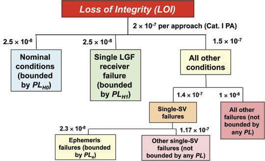
To understand how specific risk differs from average risk, it helps to start with a fault-tree representation of risk in which loss of integrity (LOI) can result from any of the nodes of the tree. Figure 2 shows a simplified example of a fault tree for CAT I GBAS. It shows the allocation of the CAT I total integrity risk requirement of 2 × 10^-7 per approach to the various possible causes of integrity loss. In specific-risk analysis, each type of failure shown in the tree, if deemed to be a credible failure (meaning, in practice, that its assumed prior probability is larger than compared to its allocation in the fault tree), is assessed that the failure is guaranteed to occur in a worst-case fashion. This means that the variables that describe this particular failure scenario take the values that maximize the hazard to users. In an average-risk analysis, these variables would take many values according to their own probability distributions, and these distributions would be convolved together to provide an overall representation of risk under that scenario. Instead, one scenario drives the specific risk assessment for a particular user class, and it is the worst one possible from that user’s standpoint. (Another user class would be evaluated under a different set of parameters corresponding to the separate worst case for that user.) The improbability of the worst-case combination of parameters is not considered as long as the probability of the failure scenario as a whole is deemed high enough to be of concern.

Figure 2. Fault tree for CAT I GBAS integrity.

Since GNSS augmentation systems contain multiple levels of health monitoring, the worst-case scenario is usually the one that maximizes the probability of an undetected hazardous error for a particular user class. Hazardous error is typically defined as any error that exceeds a pre-defined safety zone known as an alert limit (AL) or any error that exceeds the computed protection level (PL), which allows integrity to be defined separately from the intended application. Both definitions are conservative in that all errors exceeding AL or PL are treated as equally hazardous. In other words, an error just above AL is treated as just as dangerous as an error of 10 × AL. They are also misleading when used in specific-risk analyses because the resulting worst-case conditions are those that give errors just above AL or PL, as these are the generally hardest for monitoring algorithms to detect.

The use of specific risk in aviation is an evolution of deterministic guidelines for tolerable risk that date back to an earlier era when flying was more dangerous. It remains dominant in aviation safety assessment because it is partly responsible for the development of safer and more reliable air transportation. However, it has several important weaknesses compared to average risk. The first is that the degree of risk aversion preferred for aviation is buried within the hazard probabilities generated by specific risk — it cannot be separated out. This means that specific-risk results do not translate well to other classes of users, as very few users would happen to have the same risk preferences that have evolved within aviation over several decades. In addition, specific risk makes a distinction between unknown events that could be known and those that are both rare and completely unknowable. A very risk-averse value of information is much different than the risk-neutral one built into PRA, as it severely penalizes systems that do not include all potentially-informative sensors. Since each sensor added to a system provides less benefit than the last, almost all cost-effective systems choose to include less than the maximum possible number of sensors.

The conservatism implicit in specific-risk assessment severely penalizes users. Although PRA would show that the combination of factors (shown in an example induced by extreme ionospheric spatial decorrelation) needed to produce a 40-meter error in a CAT I GBAS system is exceedingly improbable (almost certainly below 10^-10 per approach), specific risk forces a significant part of the GBAS risk-mitigation effort to be targeted at this scenario. In this case, since monitoring is not guaranteed to detect the anomaly in time, the only recourse is geometry screening, a cumbersome technique in which the ground system continually evaluates the worst-case error and, if it exceeds a 28-meter tolerable limit at the CAT I decision height, determines which broadcast parameters to inflate such that all satellite geometries causing worst-case errors exceeding 28 meters are made unavailable (because the inflated VPL is larger than the 10-meter CAT I VAL). The result of this procedure is much lower user availability than would be achieved without inflation. SBAS pays a similar penalty, as we will see later. The broadcast grid ionospheric vertical error values that bound worst-case ionospheric errors (and thus the resulting protection levels) are much higher than they would be if the unusual combination of factors needed to create the worst-case error scenario were not the dominant concern.

To the extent that loss of availability represents a safety issue at the airspace level, the worst-case focus that results from specific risk is not optimal even from a safety standpoint. But this is not the only concern. Specific risk requires a great deal of development and testing to identify and mitigate a handful of very peculiar, non-representative conditions. When schedule and resources are limited, other potential threats that are easier to foresee but seem extremely improbable are often neglected. One example is the treatment of multiple hardware failures. If individual failures are assumed to be statistically independent, the probability of multiple simultaneous failures is very small. However, while statistical independence is a common assumption in probability classes because it makes calculations easier, it rarely applies in the real world. Because satellites and ground receivers are similar, if not identical, the presence of a failure in one unit may suggest a common cause or at least a common vulnerability, meaning that the probability of additional failures is much higher than independence would suggest. Thus, assuming independence by default could lead to neglecting entire categories of risk that are more threatening than the worst-case events that dominate specific risk.

Maximum WAAS Errors, Protection

To investigate the conservatism built into SBAS and GBAS specific risk assessment, maximum WAAS horizontal and vertical position errors over time (as measured by the Performance Analysis Network (PAN) maintained by the William J. Hughes FAA Technical Center) have been examined and compared to the protection levels computed when the maximum errors occurred. This study begins with PAN Report #8 (covering January to March 2004 — shortly after WAAS commissioning in mid-2003) and extends through PAN Report #34 (covering July to September 2010). Each PAN report covers three months of observed WAAS performance.

Figure 3 shows the 38 WAAS reference stations (WRSs) used by the PAN to collect position error and protection level information (some of these stations were not active in 2004 and thus were not used in earlier PAN reports). While measurements from these stations are used to generate WAAS corrections and error bounds, they are also used by the PAN as static pseudo-users that compute WAAS-corrected positions and protection levels according to the aircraft user algorithms specified in the WAAS MOPS. The resulting positions are compared to the known, pre-surveyed positions of each station to derive estimates of vertical and horizontal position errors (VPE and HPE) once per second.

Figure 3. WAAS PAN reference station network.

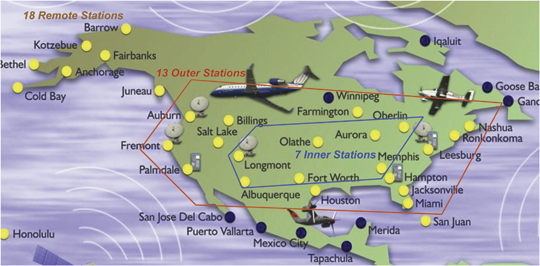
Figure 3 groups these stations into three sets of stations based on their presumed quality of WAAS coverage. These sets are unofficial and were created for the purposes of this study. The seven stations in the inner set are expected to have good WAAS coverage at all times because they are surrounded by other stations. The 13 stations in the outer set are expected to only have acceptable coverage because s
ome of them are at the edges of CONUS. The remote stations provide coverage to the inner and outer regions as well as the best possible coverage of their own regions. Because the remote stations extend beyond the primary coverage region of WAAS in CONUS, errors at these stations are not considered here.

Figure 4 is a 2-D plot of position error versus protection level in the vertical axis (that is, VPE versus VPL) for all epochs and stations during the three months covered by the recent WAAS PAN Report #34 (July 1–September 30, 2010). These results are typical of the entire period since WAAS commissioning in 2003, particularly the last several years. The vertical lines on the plot indicate the 95th-percentile, 99th percentile, and maximum VPEs in this period (1.2, 1.8, and 7 meters, respectively). The maximum VPE occurred at Barrow, AK, which is one of the most remote stations in the WAAS network (see Figure 3). In comparison, the lowest VPLs (intended to be 1–10^-7 bounds on VPE) are in the range of 10–15 meters, and values as high as 40 meters are not uncommon. The most demanding approach operation that WAAS supports, LPV-200, allows approaches to a 200-foot minimum decision height and requires that VPL be below a vertical alert limit (VAL) of 35 meters. HPL must also be below a horizontal alert limit (HAL) of 45 meters. When this is not the case, the approach operation is not available; thus these higher VPLs extract a significant cost.

Figure 4. WAAS vertical protection level versus vertical position error (June–September 2010).

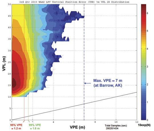
Figure 5 and Figure 6 (for vertical and horizontal errors, respectively) span the entire period of WAAS PAN Reports used in this study. VPL represents the VPL at the station and time of the maximum VPE; it is not the largest VPL recorded at a particular station. The horizontal errors shown in Figure 6 are defined analogously. Note that the station that observes the largest horizontal error in a given PAN report may differ from the one that observes the largest vertical error.

Figures 5 and 6 demonstrate that, while both 95 percent and maximum errors are quite low and are within the expected range of each other, the protection levels associated with the maximum errors greatly exceed them. This pattern is clearer in Figure 5 for vertical errors because maximum VPL tends to be more consistent across PAN reports, but it is true for horizontal errors as well.

Figure 5. WAAS vertical errors and protection levels from 2004–2010.

Figure 6. WAAS horizontal errors and protection levels from 2004–2010.

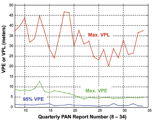
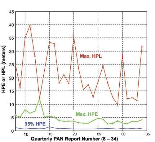
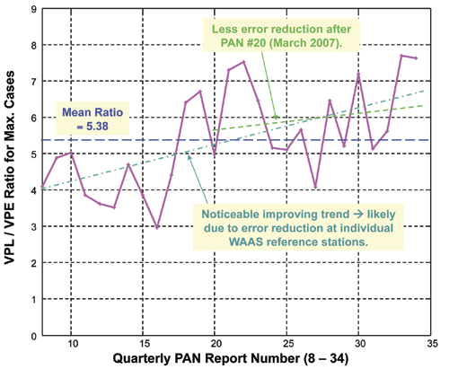
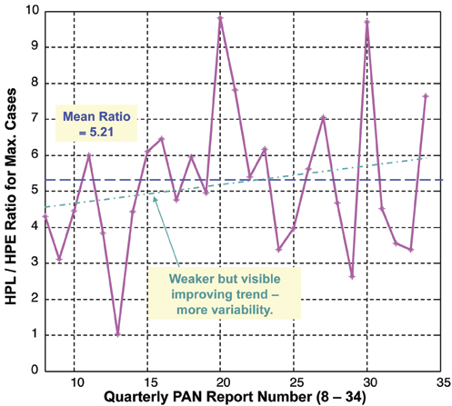
Figures 7 and 8 clarify this relationship by plotting the ratio of VPL to VPE and HPL to HPE for the station and time of the maximum error. The mean of this ratio is very high and is about the same in both cases: 5.38 for vertical and 5.21 for horizontal. Figure 7 shows a steady upward trend in the ratio that is mostly due to WRS improvements that resulted in maximum VPE being reduced over time. This trend is clearly visible in Figure 5 and appears to exceed the weaker trend of lowering VPL due to WAAS algorithm enhancements. The same trend is visible in the horizontal Figures 6 and 8 but is weaker due to the greater variability of maximum HPL over time.

To evaluate the significance of the large PL-to-max-PE ratios in the WAAS PAN database, we need to approximate the number of independent samples from which the maximum errors were derived. As noted before, WAAS protection levels represent error bounds at the 1–10^-7 probability level based on specific risk. With one measurement being collected at each operational station every second, a total of about 4.25 billion samples were collected in the PAN reports from January 2004 to September 2010. Note that measurements from remote stations are included in this count, but they are also represented in the conclusions because their PL-to-max-PE ratios are very similar to the ones shown in Figures 7 and 8. Translating this number into the number of statistically independent samples depends on the interval between independent measurements. Because both nominal and rare-event errors affect this interval, it is hard to estimate. Our best guess is a range between roughly 30 and 150 seconds, suggesting that the PAN database contains between 2.8 × 10⁷ and 1.4 × 10⁸ independent samples. Both of these numbers suggest that WAAS protection levels are very conservative from the perspective of average risk.

Figure 7. Ratio of VPL to VPE from 2004–2010.

Figure 8. Ratio of HPL to HPE from 2004–2010.

Adjusting for Average-Risk Users

Using the above results, a preliminary estimate of the reduced WAAS protection levels that would apply to average-risk users can be made. Figure 9 shows a comparison between the actual 95 percent WAAS VPL and HPL and the adjusted VPL and HPL potentially achievable with WAAS (for the same 1–10^-7 bounding probability) for average-risk users. The actual WAAS VPLs are taken from the more recent WAAS PAN Reports starting from #24 (covering January to March 2008) as the period from 2008 to 2010 includes most of the WAAS algorithm improvements introduced since commissioning in 2003. The actual 95 percent VPLs and HPLs represent the largest reported 95th-percentile values among the stations within CONUS for each quarterly period. The lower adjusted VPLs and HPLs are derived by dividing each VPL by a factor of 4.0 and each HPL by a factor of 2.5. These two reduction factors are derived from Figures 7 and 8, respectively, as conservative estimates of the ratio between protection levels and maximum position errors. Note that the factor of 2.5 for horizontal errors does not include the 12-meter error in Cleveland from PAN Report #13, as this is thought to be spurious (that is, not representative of actual WAAS behavior).

Figure 9. Projected WAAS protection level reductions for average-risk users.

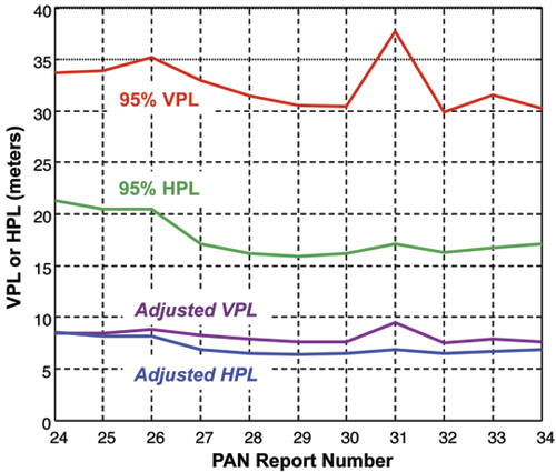
While projections based on these reduction factors are imprecise, they demonstrate the much lower error bounds that non-aviation users with an average-risk safety perspective could achieve. Most non-aviation users operate on land or sea and will be primarily concerned with horizontal error bounds. Figure 9 suggests that the typical 95th percentile WAAS HPLs of 15–20 meters (for the worst location in CONUS) can be reduced to 6–8 meters and still provide a confident 1–10^-7 error bound.

It is important to emphasize that these preliminary projections for average-risk users are just that. In order to formally establish new integrity requirements and protection levels for existing systems, the hazardously misleading information (HMI) analyses previously done for these systems need to be redone using the principles of PRA and average risk. While the original development of the WAAS and LAAS HMI analyses was lengthy and resource-intensive, almost all of the detailed work is already complete. As long as the original analyses are available, it is a much smaller task to take these results and create PRAs out of them by extracting the original specific-risk assumptions and applying average-risk principles instead.

LAAS Users. Since the first GBAS ground station design (the Honeywell SLS-4000 LAAS Ground Facility) was certified for CAT I use in 2009 and has not yet been approved for operations at a specific airport, much less data is available to do a preliminary analysis for GBAS similar to the one done for WAAS above. However, the degree of sigma inflation in the parameters broadcast by CAT I LAAS is approximately known, meaning that it can be more-precisely removed from the current LAAS protection levels to estimate what they would be for average-risk users.

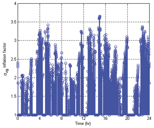
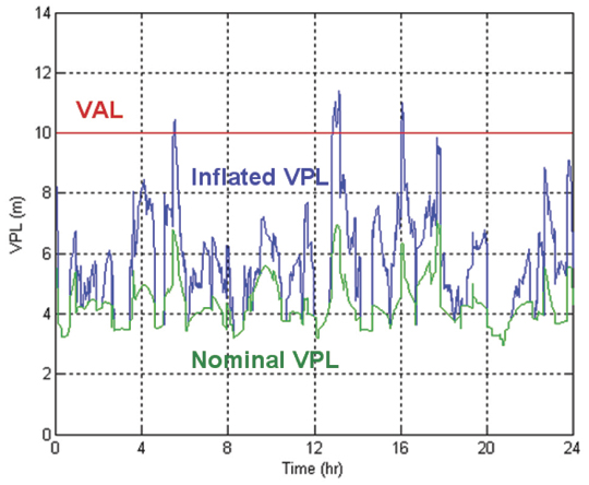
Figure 10 shows the degree of inflation applied to the broadcast σ_{vertical_iono_gradient} (or σ_vig) parameter in order to protect against the worst-case ionospheric anomaly described previously. This result is for the SPS-standard 24-satellite constellation over a 24-hour period at the LAAS installation at Newark Airport, New Jersey (the method used by the Honeywell SLS-4000 is somewhat different). While not all epochs require inflation, a majority cause the nominal σ_vig value to be increased by a factor of 2 or more, which significantly decreases CAT I availability and currently makes it impossible to take advantage of the Differentially Corrected Positioning Service (DCPS) for non-CAT-I operations.

Figure 10. Typical σvig inflation factors for CAT I LAAS.

Because of the extreme rarity of the worst-case event that dictates this inflation, it would likely not be needed for average-risk users. Figure 11 shows how much the σ_vig inflation in Figure 10 increases the LAAS VPL at Newark for the standard 24-satellite constellation. The VPL reduction from removing the inflation is not as dramatic as the potential reductions shown for WAAS in Figure 9, but they are significant relative to the 10-meter VAL for LAAS CAT I approaches. Furthermore, the pre-inflated nominal value of σ_vig for LAAS is 6.4 millimeters/kilometer, which is much higher than the actual one-sigma nominal gradient value of 1–2 mm/km because, under specific risk, the very worst nominal data must be bounded (also, worst-case tropospheric gradients must also be bounded by σ_vig). Other broadcast parameters that affect VPL, such as σ_{pr_gnd} and the ephemeris P-value that bounds worst-case ephemeris failures, would also be reduced significantly by switching to average risk. Overall, it is likely that LAAS protection levels based on average risk would be reduced from the current specific-risk PLs by about the same range of factors (2–5) observed from WAAS data.

Figure 11. Impact of σvig inflation on LAAS VPL.

User Performance Improvements

This discussion assumes that most non-aviation users who are not encumbered by the history of aviation standards development will prefer to quantify risk using PRA and the average-risk approach. As noted earlier, average risk better matches most users’ intuitive understanding of uncertainty and has the enormous advantage of separating risk quantification from risk aversion. Regardless of how risk-averse or conservative a given operator is, his or her model of risk aversion can be applied most efficiently to a risk-neutral calculation of risk that fairly represents all aspects of uncertainty. Inserting risk aversion into the calculation of risk, as done in the specific-risk approach, is both inefficient and non-optimal from a safety perspective because extensive focus on a few extreme worst-case events drives attention away from other events.

The HPL reductions for average-risk users illustrated here would be significant for many classes of ground and marine transportation users. They would allow operations with tighter physical safety margins to be supported. Users who gain no particular benefit from tighter protection levels would still obtain much higher availability of integrity, as a 25-meter HPL could be supported by much poorer satellite geometries than would otherwise be the case. In other words, users that can tolerate 25-meter horizontal error bounds would be able to operate safely a much higher percentage of the time, because the degree of GNSS constellation deterioration needed to exceed this limit would occur much less often. These benefits do not only apply at the 1–10^-7 probability level, as they would scale to the higher probabilities (1–10^-4 to 1–10^-6) that many non-aviation applications would be most concerned with.

While very few non-aviation users of GNSS today have real-time safety requirements similar to those of civil aviation, the number of such users will likely increase as the coverage of augmented GNSS (and the availability of integrity from standalone receiver-autonomous integrity monitoring, or RAIM) expands. The evolution of standalone civil GPS usage provides a precedent: as basic GPS accuracy improved from tens of meters to several meters, and the cost of user equipment dropped, more and more uses were discovered. A similar, although smaller-scale, trend is likely to occur as the advantages of augmented GNSS become more available and better understood. The primary beneficiaries are likely to be intelligent road-transport systems, train services, and marine transportation in restricted waters.

One application where tight real-time integrity bounds would be useful is in harbor and marina entry and exit; see Figure 12, taken from a Google map of a marina in San Diego, California. Based on the earlier analysis, two typical 1−10^-7 horizontal protection levels are shown: 18 meters using the unchanged WAAS MOPS approach, and 7 meters based upon modifying the broadcast bounding parameters to represent average risk (these HPLs are bounds on error in either direction, positive or negative; thus the 2-D error bounding circle has a diameter of twice the HPL).

Figure 12. Example of reduced protection levels for harbor/marina access.

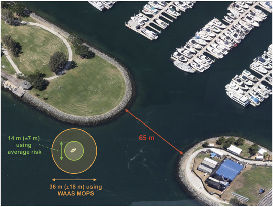
When the resulting error bounds are compared, the relative advantage of the smaller bound for this application is immediately apparent. In general, when HPL is significant compared to potential obstacles, its significance varies with the square of HPL rather than HPL itself, as the area being protected matters more than either linear direction. In this example, the ratio of HPLs being compared is 18/7, or 2.57, but the ratio of HPL-squared is much larger: 182/72 = 6.61.

When real-time integrity is not needed, augmented GNSS provides an easy means to guarantee or certify vehicle locations after the fact with great precision and reliability, without the need for post-processing. Vehicle and cargo tracking based on standalone GPS is common today, a certification of the correctness of the tracking data to probabilities suitable for legal or commercial guarantees is lacking. For this, error bounds at 1–10^-4 to 1– 10^-6 probabilities are likely sufficient, and would allow HPLs of below 5 meters from WAAS and below 3 meters from LAAS. In some scenarios, the difference between a 5-meter and a 15-meter guarantee would be minor, but in others, it could make a substantial difference.

As noted earlier, even for uses where the required HPL (as represented by the safe error limit, or HAL, for a particular application) is satisfied by the existing WAAS and LAAS protection levels, the use of modified average-risk protection levels increases the availability of integrity, which is most often expressed as the probability or percentage of time (over all satellite geometries and othe
r variable system states) that the integrity requirement is met throughout an operation (in simple terms, that HPL ≤ HAL). For user locations within good WAAS or LAAS coverage, the most variable element over time is satellite geometry. Decreasing HPL by a factor of 2.5 or more substantially increases the margin between HPL and HAL and makes it far less likely that the satellite geometry will degrade to the point where HPL exceeds HAL. For example, if the unmodified WAAS HPL equals HAL at an (un-weighted) HDOP of about 1.5, the resulting satellite availability (an upper bound on overall availability) for the SPS-standard 24-satellite GPS constellation would be roughly 98.5 percent. This means that the satellites in view (in this case, all satellites above 5 degrees elevation at a location in CONUS) would provide HDOP ≤ 1.5 about 98.5 percent of the time. However, the modified average-risk HPL (using the factor-of-2.5 reduction) would roughly translate into a limiting HDOP of about 3.75. This allows the required integrity bound to be satisfied by much poorer GPS geometries and gives a satellite availability of greater than 99.9 percent. Thus, when integrity is needed, this much greater availability of integrity is a major advantage.

Summary

SBAS and GBAS broadcasts are freely available to all GNSS users, most of whom will have different definitions of acceptable risk. These users are not optimally served at present and may hesitate to take advantage of SBAS and GBAS as a result.

Using years of collected data for the FAA WAAS system and analysis of the inflation factors built into the CAT I version of the FAA LAAS system, it appears that average-risk users of WAAS and LAAS would be adequately supported by protection levels that are 2 to 5 times lower than those currently derived by aviation users. The fact that two different approaches used to examine WAAS and LAAS suggest similar levels of over-conservatism lends credence to these estimates. While further validation by full-scale probabilistic risk assessments is necessary, we conclude that non-aviation users willing to accept average risk would obtain much better performance and availability from simple modifications to the existing SBAS and GBAS protection level calculations specified for aviation users.

Acknowledgments

We thank the FAA Satellite Navigation Program Office for its support of our research on WAAS and LAAS. However, the opinions expressed here are solely our own. We thank Jim Kelly and Tim Murphy for their explanations of the evolution of today’s SBAS and GBAS integrity requirements. We also thank the FAA Technical Center for its efforts in collecting and publishing WAAS error data over the last decade using its Performance Analysis Network (PAN).

Sam Pullen is a senior research engineer at Stanford University, where he is the director of the Local Area Augmentation System (LAAS) research effort. He has supported the FAA and others in developing GNSS system concepts, requirements, integrity algorithms, and performance models since obtaining his Ph.D. from Stanford in Aeronautics and Astronautics.

Todd Walter is a senior research engineer in the Department of Aeronautics and Astronautics at Stanford University. He received his Ph.D. from Stanford and is currently working on the Wide Area Augmentation System (WAAS), deﬁning future architectures to provide aircraft guidance, and on assuring integrity on GPS III.

Per Enge is a professor of aeronautics and astronautics at Stanford University, where he is the Kleiner Perkins, Mayﬁeld, Sequoia Capital Professor in the School of Engineering. He directs the GPS Research Laboratory and received his Ph.D. from the University of Illinois.

July 1, 2011
Lone Sentinel: Single-Receiver Sensitivity to RF Interference
By Jenna R. Tong, Robert J. Watson, and Cathryn N. Mitchell, University of Bath

Using signal-to-noise measurements from a single commercial-grade L1 GPS receiver, it is possible to detect interference or jamming that is above the thermal noise floor and below a power that causes loss of position.

Interference, intentional or unintentional, is an acknowledged vulnerability of GPS systems. Many of the potential sources of interference are unintentional: interference can caused by harmonics of out-of-band signals, electronic noise, or malfunctioning equipment. The effect, however, is the same independent of intent.

The presence of high-power interference which causes continual denial of service is fairly easy to detect, but lower power interference may still degrade performance, for example by causing loss of lock on some satellites, thus increasing position dilution of precision, although the receiver continues to output a position. Short periods of denial of service caused by intermittent high-power interference may not be immediately detected depending on the timing and ability of the system in use to deal with temporary loss of signal.

Therefore, to fully characterize an antenna environment requires a 24/7 system, whether the purpose is to determine whether a location is suitable prior to installation, to identify whether problems at an existing site are due to interference, or to provide warnings of the presence of interference on a continuous basis. In particular, information on timing — for example finding a time of day or day of the week when interference is regularly seen — may assist in determining the source of the interference.

This research forms part of the GNSS Availability Accuracy Reliability anD Integrity Assessment for timing and Navigation (GAARDIAN) project, which provides a mesh of sensors to monitor the integrity, reliability, continuity, and accuracy of the locally received GPS (or other GNSS) and eLoran signals continuously and to detect anomalous conditions such as local interference, differentiating between possible sources of errors such as interference, multipath, satellite errors, or space weather.

Here we look at using the signal-to-noise ratio (SNR) values from a single-frequency GPS receiver to detect interference. There are two stages to the algorithm: determining the local environment of the antenna in terms of multipath and interference, and identifying and recording potential interference events.

Since this method uses values output from a GPS receiver, characterizing the response to interference of the receiver used in the probe is necessary, to indicate what level interference can be detected with the system, as well as ensuring that false positives are not produced, and the effects of interference can be separated from those of multipath and scintillation, which can also cause decreases in SNR.

We used a commercial, single-frequency receiver, recording this data from NMEA messags for analysis:
- SNR, in dB, reported as an integer
- elevation, in degrees, reported as an integer
- azimuth, in degrees, reported as an integer
- carrier lock time, in seconds.
Algorithm. To determine the presence of interference, the normal state of the receiver must first be calculated. Initially it is assumed the receiver is fixed with an unchanging multipath environment. SNR and elevation values from all satellites are accumulated for several hours. To reduce influence of the unknown multipath environment, values from satellites below 10 degrees elevation and from those where the carrier lock time is less than four minutes are removed from the data set.

A polynomial fit between elevation and SNR is then calculated from the remaining data. A second- or third-degree polynomial generally fits the high-elevation data with deviations from the profile at low elevations being primarily due to multipath where interference is not present.

The standard deviation of SNR at each elevation is then calculated. The combination of the polynomial and these values of standard deviation characterize the normal environment of the receiver, for the case where interference is not present in the data gathered (Figure 1).

Figure 1. Raw SNR data against elevation, for all satellites in view over a period of 12 hours (blue), and a polynomial fitting to the same data (green).

To confirm that the threshold values returned by the first stage of the algorithm are valid, a value is calculated for the elevation where the SNR value drops below the polynomial curve by the greatest amount.

If interference is not present, this is normally found at the point where multipath begins to influence the incoming signal and can be considered as a rough multipath cutoff, used to remove signals that may be influenced by multipath from later stages of the analysis.

Assuming a well-sited antenna, a value greater than 25 degrees for this value indicates the possible presence of interference in the data used to calculate the polynomial. In cases where this value is high, the data in question would be rejected, and optionally a user may be warned that there may be pre-existing interference. If the antenna-receiver combination has been previously calibrated in a known good environment, it would be also possible to identify interference based on the difference in polynomial and standard deviation values between that environment and the location being tested.

Figure 2 shows the value of this multipath cutoff (in degrees) for a set of data where interference was known to be present initially, against the start time for the data used to calculate the polynomial and multipath cutoff values, by number of hours from the start of the file.

Once the mask is developed, a threshold value can be set to be n standard deviations below the polynomial, and events are detected by the combination of:
- At least four satellites with elevations above the multipath cutoff which are below the threshold value or which were above the multipath cutoff previous to losing lock.
- This status is continuous for more than a set time t.
Requiring multiple satellites limits the effects of other influences on SNR such as multipath; requiring an extended time period removes very short-term fluctuations.

The number of false positives and the power of interference required to cause an alarm then depends primarily on the value of the threshold factor n, and on the time period t, which here we kept at a constant of 30 seconds.

Testing

To avoid radiating interference, we constructed an RF network to facilitate injection of jamming signals into the GPS signal path. The GPS signal from a roof-mounted choke-ring antenna was passed through an amplifier and attenuator chain to provide 0 dB forward gain, but around 40 dB reverse isolation. An additional stepped attenuator (0–40 dB in 1 dB steps) was also included. The buffered signal from the antenna was then combined with the output of a vector signal generator used to provide the jamming signal.

The combined signal was then fed into the GPS receiver via a DC-block to remove the antenna bias voltage. The signal generator is capable of producing a wide variety of jamming including matched spectrum wideband noise, CW, and pulsed signals. The adjustment of both the signal generator output power and the signal attenuator a
llow the replication of a variety of signal-to-noise and jammer-to-noise scenarios.

With the receiver locked onto a stable position, CW signals at L1 frequency were introduced into the receiver at levels from –125 dBm to –90 dBm in steps of 5 dBm, with at least 15 minutes of buffer time for the receiver to recover between each step (Table 1). Data was logged at 1 Hz throughout. We collected 20 hours of data, to calculate threshold values from data with no known interference.

Table 1.

Results

Twelve hours of data from a period where no known interference was present was used to form the SNR mask, and events longer than 30 seconds were looked for using various values of n for the threshold across all 20 hours of data. A false alarm was considered to be any event where interference was detected while the signal generator was off. Table 2 summarizes the response for different threshold levels.

Table 2.

In this test, CW interference of –100 dBm was required before the number of satellites with carrier lock dropped below four even for a single epoch, and –90 dBm was required to cause a sustained loss of lock, but jamming of –105 dBm was still detectable by this system with no false positives returned.

Decreasing the threshold began to produce false positives without detecting the smaller interference signals. This is not surprising as the thermal noise floor, assuming 2 MHz bandwidth, is about –110 dBm.

In the raw data from the detected events, a sharp dip in SNR is often seen at the beginning of an event, followed by recovery as the receiver compensates. In this particular case, where the aim is to detect the interference, this could lead to interference going undetected if the initial sharp dip was underneath the time threshold (30 seconds) and the recovery took the SNR of some of the satellites above the SNR threshold (Figure 3).

Figure 3. Value of polynomial mask (blue) and actual SNR (red) as recorded for four satellites during the period around the injection of the -100 dBm CW signal, showing initial dip and partial recovery.

Conclusion

Using only SNR values from a low-cost L1 GPS receiver, it is possible to detect CW interference which is above the thermal noise floor and below a power that causes loss of position. Different types of interference are expected to produce a different response, and unintentional interference is likely to be broadband or not directly centered on L1. The antenna used may also have a strong effect. These factors have not been examined here, although in practice the algorithm has run in multiple locations with different antennas, both direct and via splitters.

Regardless of the precise type of interference, the system would be expected to detect any interfering signal which impacts the SNR of the receiver, and to do so even if the signal strength was below a level which caused denial of service in that area.

The results are specific to the receiver used and its response to interference, although the algorithm would be capable of using data from any receiver that provided SNR values. Ideally the system used for measurement would have little or no built-in interference rejection.

Although this data was collected and then examined after the fact for signs of interference, the system works in precisely the same way in real time. Further trials will test the algorithm’s performance in real time and with different jamming scenarios, and compare results from multiple receivers in a single location and the performance of the algorithm with different antennas.

Acknowledgments

This work was funded by the Engineering and Physical Sciences Research Council and the Technology Strategy Board.

Manufacturers

Single-channel receiver, Chronos Technology CTL430; vector signal generator, Rohde & Schwarz SMIQ03.

Jenna R. Tong is a postdoctoral researcher in electronic and electrical engineering at the University of Bath. Her Ph.D. in electron tomography is from the University of Cambridge.

Robert J. Watson received a Ph.D. degree in electronic engineering from the University of Essex, and is senior lecturer in electronic and electrical engineering at the University of Bath.

Cathryn N. Mitchell is a professor of engineering at the University of Bath and the Director of Invert Centre for Imaging Science. She received a Ph.D. from the University of Wales Aberystwyth.
July 1, 2011
Letters to the Editor: LightSquared Satellite Case Skimpy

LightSquared Satellite Case Skimpy

Thank you for the story “LightSquared, FCC Rebuttals Distort Record.” One thing worth clarifying: you state, “It appears that the purpose of Lightsquared’s satellite service is, now, to provide ancillary service in remote areas not covered by the ubiquitous primary terrestrial network, or in the event that the terrestrial network is destroyed — exactly the opposite of what the FCC authorized and the GPS industry had understood and agreed to.”

But even this can’t work unless they are going to limit the number of subscribers in remote areas. A 4G user will expect decent wireless data throughput, but the subscriber’s connection is shared with other users within a spotbeam covering a large area. All connections must fit within the bandwidth of the single beam.

Cell networks get around this problem by frequency re-use, possible since each cell covers a small geographic region. The key characteristic of a cellular network is the ability to re-use frequencies to increase both coverage and capacity.

Admittedly, the LightSquared satellite, SkyTerra-1, is a very sophisticated space vehicle with a record 500 spotbeams. However, it provides a maximum user data rate of 300–400 Kbps, quite a bit short of what you would expect from a 4G-LTE connection. And at 400 Kbps, a 20-MHz spotbeam could still support only 50 to 100 connections.

Another problem with using the satellite link is that although they have managed to solve the problem of requiring a special user handset, the user will still have to be outdoors and in the open to communicate with the satellite. And it is a geostationary satellite, which means high latency — at least 1/4 second. Using this for voice would create user annoyance.

LightSquared should stop using the word “ancillary” and stop pretending that their network has a significant satellite component. It is going to have to be all ground-based if they are to provide 4G connectivity. It’s really starting to sound like the satellite is just a way for LightSquared to meet their FCC requirement.

— Mike Whitehead
VP Technology, Hemisphere GPS
[Ed: citations and some discussion ommitted for space; available on request.]

On Eric Gakstatter’s Survey columns:

Keep up the good work. I find your e-newsletter columns the best way to stay informed [on the LightSquared issue].

— editor, survey magazine

Sounding Off

When someone comes onto the basketball court with a hockey stick, the referees should not negotiate rule changes. Anything that allows LSQ to proceed either on the high or low ends of their allocated spectrum will in the long run be a blow to PNT users and suppliers worldwide. While this may very well end up as a compromise to the detriment of us all, now is not the time to concede any ground. He who flinches, loses, and this is not the time for engineers to give ground. It will set a precedent that lawyers will use again to decimate the spectrum in the future.

—Informed particpant

July 1, 2011
Expert Advice: Critical Offshore Applications of SBAS GNSS

James D. Litton, President/CEO, Litton Consulting Group

Precise positioning of many different kinds of vessels and other equipment depend upon satellite-based augmentation systems (SBAS) of GNSS, principally GPS and GLONASS at this time. The applications range from exploration to production and delivery of hydrocarbons to shore-based installations and navigation of very large crude carriers, or oil tankers. Decisions and recommendations are strongly needed to keep these services free from interference.

It is fallacious to think that because LightSquared or similar use of out-of-band high-power terrestrial radiation would be confined to a continental region (physically impossible, in any case), that no harm would accrue to offshore navigation assets. The three principal suppliers of these offshore precise positioning services are Fugro’s Starfix services, C&C Technology’s C-Nav which utilizes John Deere/NavCom’s StarFire systems, and Subsea 7’s Veripos system.

All of these systems depend upon GNSS reference receivers placed around the world in networks which depend upon corrections that are derived from regionally sited reference stations. The 10-centimeter level of precision now required for many of the most dangerous and valuable applications requires, in turn, centimeter-level accuracy in base stations in the United States and elsewhere in the world.

Inmarsat frequencies allocated to these applications for delivery of the differential corrections generated by these reference stations have been in use for both the huge number of land applications (agriculture, infrastructure development, river and harbor navigation, seismic exploration, pipeline surveys, etc) and offshore applications. Changing these frequencies is feasible only at great cost to both Inmarsat and the many on- and offshore uses. Inmarsat may be compensated by LightSquared for its costs, but not so the many millions of dollars of expense to offshore and onshore operators in down time, redesign and reprogramming of receivers, and suspension of critical operations.

The offshore applications outlined here are just a few of the more familiar. No attempt has been made to capture all of these applications in this short memorandum, but operators in this industry, represented by the National Ocean Industries Association (NOIA), have made their position clear in the attached letter to the FCC.

Major Offshore Applications

Exploration. Modern seismic exploration depends upon seismic streamers many kilometers long. Several such streamers (containing thousands of hydrophones for capturing reflections from deep beneath the ocean floor and determining the structure and composition of the strata which may contain hydrocarbons) are towed by each ship. The seismic profiles which result are depicted in three dimensions with great precision. Discovery and assessment of such strata depend sensitively upon the positioning accuracy of these streamers, which, in turn, depend sensitively on the position of the vessel with respect to the center of the earth, because the vessel’s trajectory is the reference for the relative positioning of the streamers by magnetic and inertial means, sometimes augmented by GNSS receivers integrated into the seismic streamers.

Drilling. Increasingly, drill rigs and drill ships are placed and maintained in position by dynamic positioning systems that depend upon augmented GNSS systems for stabilizing the massive structures over the well head. In deep water (more than 5,000 feet), only dynamic positioning through the use of massive thrusters (such as those employed by the Deepwater Horizon vessel of Transocean in the Macondo well disaster, commonly referred to as the BP disaster) is feasible. With as much as 10,000 feet of riser attached to these drill ships between the well head and the ship, safe operation is critically dependent upon very precise positioning of the vessel. Further, down-hole positioning depends upon inertial and wireline systems, which are calibrated by the use of augmented GNSS systems.

Production. Production platforms range from single sites over a single well to massive platforms with undersea pipelines and risers connecting them to manifolds on the sea floor, which in turn are connected to multiple well heads in an area. This infrastructure is placed, maintained, and monitored with the use of SBAS systems integrated with acoustic systems. Use of remotely operated vehicles and autonomous underwater vessels or vehicles, submarines equipped with sensors that can image and manipulate underwater structures, for these purposes is prevalent.

Station Keeping. Supply vessels, crew vessels, special-purpose vessels, and helicopters are positioned relative to the drill rig, seismic vessel, production platform, and pipeline-laying vessel by SBAS systems fused with other sensors such as lasers and microwave distance-measuring equipment. A huge drill ship, for instance, moving about in response to ocean dynamics but centered on the well head, cannot be docked to a supply vessel solely with ropes and cables. Each vessel must be free to move but to move synchronously with each other. Because of the huge masses involved, the velocity of each relative to the other must be kept as near zero as possible. Centimeter-level precision is required for this purpose. In all of the applications listed above, at various stages, vessels require station keeping with other vessels to very precise relative distances and velocities.

Containment and Recovery. When there is a requirement for a flotilla of vessels such as attended the Macondo blow-out event, there are as many as a hundred large and small vessels in a relatively small area, with the need for central control (by the U.S. Coast Gaurd in this case) and collision-avoidance systems. These systems also depend upon having precise GNSS, mostly using SBAS systems.

Further application details and additional critical applications can be provided upon request.

Jim Litton is the President of the Litton Consulting Group, Inc. (LCG). His GPS-related experience includes being the Chief Engineer at Magnavox during the GPS phase I development, contributing to analysis of ionospheric effects and senior vice-president and general manager of the Magnavox Commercial GPS Division before forming the Litton Consulting Group in 1992. He co-founded NavCom Technology in 1994. He holds the Hays award from the ION for 1996 and is co-inventor on a codeless GPS receiver patent.

July 1, 2011
Expert Advice: Energy Production Concerns about LightSquared

Randall Luthi, President, National Ocean Industries Association

By Randall Luthi, President, National Ocean Industries Association

To: Mr. Julius Genachowski,
Chairman, Federal Communications Commission
Ref: LightSquared, Inc.,
L-Band allocations impacting GPS FCC File No. SAT-MOD-20101 1 IS-00239

Dear Chairman Genachowski:

The National Ocean Industries Association (NOIA), which represents approximately 270 member companies involved in outer continental shelf (OCS) energy production throughout the United States, is gravely concerned over the pending allocation of Mobile Satellite Services (MSS) spectrum to LightSquared, Inc. for terrestrial high-powered transmissions. LightSquared’s proposed transmission structure will adversely impact GPS and Inmarsat signals along our coastlines, both of which are critical to marine operations. Specifically, NOIA is concerned that:

1. Coastal and near shore GPS operations will be impacted even at (promised) reduced LightSquared power levels. While NOIA understands that LightSquared will be required to reduce its tower transmission power along the coastline, their reduced power transmissions will still be many orders of magnitude greater than GPS signals, virtually guaranteeing interference for users in coastal and near-shore areas.

2. GPS receiver types used by NOIA members will be impacted substantially. NOIA members primarily use high-precision GPS receivers for their high-accuracy coastal and near shore work. High-accuracy GPS receivers require a wide-band front end, which will be seriously impacted by LightSquared transmissions.

3. Inmarsat-linked DGPS corrections will have interference. Virtually all of the high-accuracy GPS work requires the use of differential GPS corrections transmitted by Inmarsat in “L” band. These corrections will be jammed by the LightSquared signal. Implications are, for example, dredging or excavation work in areas near buried high-pressure natural gas pipelines. This work will become much more dangerous due to inaccurate, intermittent, or unreliable GPS readings.

4. Offshore oil and gas operations will be impacted because of interference on land. LightSquared interference from their 40,000 proposed transmission sites across the nation will interfere with dozens of high-accuracy DGPS reference stations used to generate differential corrections for offshore use and high-accuracy operations on shore. Because of this land-based interference with high-accuracy GPS reference stations, hundreds and possibly thousands of coastal users will be impacted. High-accuracy differential GPS corrections are used by a wide cross-section of marine users including dynamically positioned drilling rigs, pipeline construction vessels, rig supply vessels and others. Loss of GPS corrections or erroneous differential GPS corrections due to shore-based interference can cause a floating drilling rig to deviate from station resulting in catastrophic blowouts, environmental damage, and fatalities.

5. LightSquared will cause interference with Inmarsat. NOIA understands that LightSquared has paid Inmarsat, and will continue to pay Inmarsat a fee, to “endure the pain” caused by the interference. However, Inmarsat’s customers, including virtually all NOIA members, will still be required to endure the pain. Isotropic Inmarsat antennas will be impacted the most. NOIA understands that Inmarsat plans to move user frequencies at their cost. However, NOIA cannot be assured that this solution is viable given the financial drivers LightSquared is offering Inmarsat; it is not reasonable to assume that Inmarsat can compensate thousands of users for the costs of making the changes, even if the equivalent frequencies and powers are available.

6. NOIA is concerned that the FCC was premature in its decision to issue a waiver to LightSquared. Unlike the FCC’s historic test-then-approve, NOIA is concerned that the FCC has fast-tracked the effort and has improperly and unnecessarily implemented an approve-then-test procedure for this applicant. NOIA is concerned that the FCC may have directed findings of the professional staff in its decision making.

7. NOIA believes that millions of land and airborne GPS and DGPS user groups will be severely impacted by LightSquared transmissions. In conclusion, NOIA and its 270 member companies are extremely concerned that high-end GPS, DGPS, and the associated GPS reference stations will be interfered by LightSquared transmissions in the band previously protected for the very low power signals typical of satellite communications. The real-time GPS positioning needs of NOIA member companies are critical to the safety and success of their operations, and although these operations are at-sea they are totally dependent on shore-based GPS reference receivers, therefore LightSquared’s land-based operations will affect the offshore regions as well. With the marine industry’s giant assets including very specialized 2 vessels of all types completely dependent on GPS, the safety and environmental implications of GPS interference is astronomical. NOIA is concerned that other specialized Inmarsat installation members will also be disrupted.

Finally, NOIA believes that the FCC is moving too quickly and needs to step back and make its decisions based on sound science, understanding that national wireless coverage is being pursued with all deliberate speed by several knowledgeable industrial groups that have paid for the value received from their frequency allocations. It does not need this asymmetric and competition-reducing spectrum grab by a group without the years of experience and trust of those who are building the infrastructure to accomplish the very laudable outcome that is ostensibly LightSquared’s motivation.

July 1, 2011
On-Site Geo-Referencing of 3D Static Terrestrial Laser Scans

By Jens-André Paffenholz

This blog presents an efficient procedure for directly geo-referencing static 3D laser scans. This is a worthwhile way to obtain the required transformation parameters from the local sensor-defined coordinate system to a global system. Therefore, a multi-sensor systems (MSS) is designed with a phase-measuring laser scanner and 3D positional sensors (see Figure 1). By means of at least one eccentrically mounted GNSS antenna on top of the rotating laser scanner one gets a 3D trajectory of the antenna reference point (ARP). The analysis of the resulting trajectory within a recursive state-space filtering approach (e.g., Kalman filter) yields the transformation parameters (position and orientation) and their full variance-covariance matrix. Apart from the geo-referencing of single laser scans the propagation of the transformation parameter variances to the point clouds is possible. Moreover, an improvement of the obtained direct geo-referencing results by means of matching algorithms (like, e.g., Iterative Closest Point (ICP) algorithm) with consideration of the stochastic point cloud information of each single 3D point is feasible.

Figure 1. Sketch of the MSS (at the Geodetic Institute of the Leibniz Universität Hannover) composed of a phase-measuring laser scanner, GNSS equipment and two single-axis inclinometers.

Overview about the enlisted sensors, their specifications and the algorithm for the transformation parameter estimation

The main characteristic of the terrestrial laser scanning (TLS) technique for engineering geodesy is the immediate data acquisition in 3D space. This is realised with a high spatial resolution (a few millimetres for mean distances of approx. 25 m), as well as with a very high frequency (up to 50 profiles per second) in a relative or local sensor-defined coordinate system. The TLS technique can be used in a static or a kinematic mode. Static scanning is characterised by one single fixed translation and orientation of the laser scanner in relation to an absolute or global coordinate system. For kinematic scanning, where the data acquisition is commonly reduced to 2D profiles, the translations and orientations are time-dependent. Hence, the transformation parameters for each profile are different in relation to each other as well as to an absolute or global coordinate system. When a combination of several static scans from different stations into one coordinate system (registration) is required, the transformation parameters for each scan have to be determined. For an additional link to an absolute or global coordinate system (geo-referencing), typically control points in a known geodetic datum are necessary. By the direct observation of the required transformation parameters by means of GNSS equipment and arbitrary navigation sensors, one can solve the registration and geo-referencing in one single step without the need of additional control points.

At the present developmental stage of the MSS (at the Geodetic Institute of the Leibniz Universität Hannover), it is composed of a phase-measuring laser scanner, one eccentrically mounted GNSS antenna and two inclinometers on top of the rotating laser scanner (cf. Figure 1). Hereby, the horizontal rotation of the laser scanner of at least 360 degrees is suitable to derive the position as well as the azimuthal orientation of the laser scanner.

Currently, the GNSS data processing is done in post processing. In general, real-time processing is possible within the purposed geo-referencing procedure. The practicability within the direct geo-referencing procedure due to expected higher variances for the trajectory points of the ARP has to be investigated in the future. However, the short high frequent trajectory of the ARP makes the GNSS analysis a challenging problem which has to be overcome. The overall duration is about 15 min with up to 20 hz data rate. In this approach the alternating antenna orientation with respect to an earth-centred earth-fixed coordinate system will contribute to the error budget due to the right-hand circular polarisation of the satellite signals and the azimuthally varying phase centre corrections (PCC). In addition, near-field effects caused by the antenna adaption (made from aluminium) on the laser scanner, or possibly multipath from the vicinity surrounding the scanner may contribute to the error budget. Investigations of these GNSS related errors yield to no significant impact of the used antenna adaption within a double difference analysis in the observation domain. As expected, the rotated PCC against the original PCC has an effect of up to 5 mm in the observation domain which corresponds to the horizontal offset components of the used GNSS antenna. The analysis in the coordinate domain also indicates an effect of up to 5 mm. The analysis shows that the PCC effect is dominated by the phase centre offset components. One can conclude that within the currently applied epoch-wise GNSS analysis the effect of rotated PCC has no significant impact on the transformation parameters in the geo-referencing procedure. For further details about these investigations please refer to Paffenholz et al. (2011).

The analysis of the 3D ARP trajectory (cf. Figure 2) is performed within an adaptive extended Kalman filter (aEKF). This yields the transformation parameters (position and orientation) alongside their full variance-covariance matrix. The benefits of using a closed form algorithm on the basis of a Kalman filter (KF) are the following: Firstly, the KF allows real-time data processing, and secondly, the parameter estimation will be less sensitive to outliers. To deal with non-linearities in the system and measurement equations, an extended KF (EKF) is used to estimate the transformation parameters of the MSS. Another promising approach for a non-linear state estimation is the combination of Sequential Monte Carlo filtering (also known as particle filter) and an EKF, which was proposed by Alkhatib et al. (2011). The main benefit of the proposed approach is the better performance in case of high-nonlinear state-space equations. An improvement of the dynamic model of the EKF can be achieved by augmenting the EKF with adaptive parameters. These parameters are time invariant and system-specific with well-known initial values. For further details please refer to Paffenholz et al. (2010).

Figure 2. Sample ARP trajectory of a 360 degree rotation of the laser scanner around its vertical axis. Red indicates the original10 hz measurements with a Javad GNSS receiver Delta with Javad GrAnt-G3T antenna. Blue and green indicate the predicted and filtered trajectory within the aEKF approach, respectively.

Performing the direct geo-referencing by applying the transformation parameters and calculation of the uncertainty measures of the 3D point cloud

The final step of the purposed direct geo-referencing procedure is to apply the transformation parameters (translation vector as well as at least the azimuthal orientation) to the 3D point cloud. The three spatial rotation parameters can be reduced to the azimuthal orientation in case of a sufficient sensor orientation to the direction of gravity. The left part of Figure 3 shows the transformation result from the local sensor-defined to an absolute coordinate system in the case of two 3D point clouds, each from a different static scanner station (red and blue). The radial distance between the scanner and the object is 15 m and 20 m, respectively. It is obvious, that the two geo-referenced point clouds have a slight misalignment of a few centimetres. Due to the known absolute coordinates of the pillar on the roof of the building (middle part of the figure), one can conclude that the geo-referencing of the blue point cloud is inaccurate. Moreover, the variances for the transformation parameters from the blue station are higher than the variances for the red station. This leads to the conclusion that the estimated transformation parameters for the blue station are not reliable. Nevertheless, this direct geo-referencing can be used as adequate pre-registration for matching algorithms.

To overcome this misalignment the application of matching algorithms, like the ICP algorithm, is worthwhile. As input for the ICP algorithm the pre-registered 3D point clouds are used. The a-priori alignment (within a few centimetres) of the two point clouds is sufficient for the application of the ICP algorithm to find an adequate amount of corresponding points for a reliable estimation of the transformation parameters. The ICP result is shown in the right part of Figure 3. One can clearly see that the matching of the two point clouds was successful. The recent topic of the ongoing research is the consideration of the uncertainties of each point cloud within the ICP algorithm for a further improvement of the matching results.

Figure 3. Left: Applied transformation parameters to two scans from different stations (red and blue). Right: Result after running the ICP algorithm on the pre-registered 3D point clouds (shown in the left part of this figure).

In the current research work uncertainties for each single point cloud are calculated by variance propagation: Combining the uncertainties of the scanner measurements (e.g., manufacturer values for the angle and range measurement accuracy), and the uncertainties of the direct geo-referencing procedure (variance-covariance matrix of the transformation parameters obtained within the aEKF). As mentioned before, these uncertainties should be considered in the ICP algorithm in the ongoing work for a further improvement of the matching results. Bae et al. (2009) already stated that the consideration of positional uncertainties in the point cloud matching will be a worthwhile approach to improve the matching, as well as the interpretation of 3D point clouds. An example for the result of the variance propagation of the scanner and direct geo-referencing uncertainties is illustrated in Figure 4. The figure depicts a stochastic point cloud of the red station (similar 3D point cloud as shown in Figure 3). As measure for the uncertainty the mean of the coordinate uncertainty in a range of 5 mm up to 30 mm is shown.

Figure 4. Stochastic point cloud of red station resulting from variance propagation for the uncertainties of the scanner measurements and the direct geo-referencing procedure. Depicted is the mean of the coordinate uncertainty.

Conclusions and Future Work

This article describes an on-site direct geo-referencing of 3D static laser scans by means of tracking the circular motion of the laser scanner around its vertical axis with 3D positioning sensors. The required transformation parameters from the local to an absolute coordinate system are estimated within a Kalman filter approach. The results show a misalignment for two different static laser scanner stations in a range of a few centimetres. Nevertheless, this is an adequate pre-registration for matching algorithms. Besides the geo-referencing, the uncertainties of the 3D point clouds are calculated by variance propagation. The future work is focused on the consideration of the stochastic point cloud information within matching algorithms (like, e.g., ICP) for an optimal fusion of different (pre-) registered point clouds into one optimal solution.

References

Alkhatib, Hamza; Paffenholz, Jens-André; Kutterer, Hansjörg (2011): Sequential Monte Carlo Filtering for nonlinear GNSS trajectories. In: Sneeuw; Novák; Crespi and Sansò (Eds.): Proceedings of the VII Hotine-Marussi Symposium on Mathematical Geodesy, Rome, 6-10 June 2009. International Association of Geodesy (IAG). 1st Edition. Berlin, Heidelberg: Springer, (in press).

Bae, Kwang-Ho; Belton, David; Lichti, Derek D. (2009): A Closed-Form Expression of the Positional Uncertainty for 3D Point Clouds. In IEEE Trans. Pattern Analysis and Machine Intelligence 31 (4), pp. 577–590.

Paffenholz, Jens-André; Kersten, Tobias; Schön, Steffen; Kutterer, Hansjörg (2011): Analysis of the Impact of Rotating GNSS Antennae in Kinematic Terrestrial Applications. In: Proceedings of the FIG Working Week 2011. FIG. Marrakech, published on CD only / also available via www.fig.net.

Paffenholz, Jens-André; Alkhatib, Hamza; Kutterer, Hansjörg (2010): Direct geo-referencing of a static terrestrial laser scanner. In JAG 4 (3), 115–126.

Jens-André Paffenholz received his Dipl.-Ing. in Geodesy and Geoinformatics at the Leibniz Universität Hannover. Since 2006 he has been research assistant and since 2008 also PhD candidate at the Geodetic Institute at the Leibniz Universität Hannover, respectively. His current interests are: terrestrial laser scanning, industrial measurement systems, and process automation of measurement systems. The present research focus is: precise direct geo-referencing in terrestrial laser scanning applications.

June 29, 2011
LightSquared Goes Global; GLONASS, Galileo May Be at Risk, Too

Recent events, some of them summarized here, may appear to have dealt setbacks to LightSquared, the boundless opportunist of wireless broadband that just happens to interfere with GPS. But the company has not run out of moves yet. Would you, if you had $20 billion at stake? The latest gambit, led by lawyers and cloaked in jargon, appears to be an end-run around the U.S. government to appeal to the International Telecommunications Union, which has ultimate and international authority over spectrum. Watch out, GLONASS and Galileo — and U.S. troops operating in foreign theaters.

GPS World has received copies of three “fact sheets” authored by two lawyers and a strategic consultant. The documents are addressed to ITU-R WP 4C, the International Telecommunications Union Working Party that handles mobile satellite services (MSS) and radio determination satellite service (RDSS spectrum) and orbits. One document is titled “ Compatibility between Complimentary Ground Componenet in the 1525–1559 Mhz and 1626.5–1660.5 Mhz Bands and Other Service.” All three documents appear to be cover sheets for longer treatises, and their language and citations are not entirely clear to me, as my legal and regulatory background leaves something to be desired.

However, they announce their purpose as “to modify and refine the example methodology to calculate aeronautical mobile satellite (route) service spectrum requirements,” and “to address ongoing Integrated Mobile Satellite Service Complimentary Ground Component compatibility matters,” and finally “to update the Integrated Mobile Satellite Service Complimentary Ground Component technical characteristics based upon the most recent information regarding CGC deployment plans in this frequency band.”

One source familiar with the documents, who did not wish to be named, commented that “One should interpret what LightSquared is doing with ITU as a bellwether indication of intent to use the whole band at the full authorized power, no matter how they spin ‘protect GPS’ in their press releases.   

“At first blush, the filings look innocuous; let me assure you, they are not. This is the first salvo. Watch what they do, much more than what they say.

  “These are fact sheets intended to inform the U.S. government that LightSquared intends to develop papers with the intent to get the U.S. government to approve the papers to be sent to the ITU WP-4C, the Working Party that handles MSS and RDSS spectrum & orbits. The ultimate goal is to work internationally to allow LightSquared to allow ancillary terrestrial component (ATC) broadcast globally.”

The three so-called fact sheets are appended here.

In other developments, going now in reverse chronological order, from most recent to early June:

Congressional Activity

On June 23, the U.S. House of RepresentativesAppropriations Committee approved the fiscal year 2012 Financial Services and General Government Appropriations bill. One amendment to the bill prohibits funding for the Federal Communications Commission (FCC) to remove conditions on or permit certain commercial broadband operations until the FCC has resolved concerns of harmful interference by these operations on GPS devices. The amendment was adopted on a voice vote. More details here.

Previously, on May 27, the U.S. House of Representatives passed a bill stating that the FCC shall not provide final authorization for LightSquared operations until Defense Department concerns about GPS interference have been resolved. The bill then went to the U.S. Senate for its action.

The House actions and a letter to the FCC signed by 32 U.S. senators may presage a showdown over the issue between Congress and the president, who has promised increased broadband access. A 4G wireless network providing this access could be facilitated by LightSquared sales of service via its tower transmitters to wireless carriers. LightSquared has already signed a $20 billion, 15-year deal with Sprint.

Money Talks

A report on “The Economic Benefits of Commercial GPS Use in the United States and the Costs of Potential Disruption” was presented by during a June 21 webinar sponsored by the Coalition to Save Our GPS. The report estimates that “the direct economic benefits of GPS technology on commercial GPS users are . . . over $67.6 billion per year in the United States,” but also that ““the direct economic costs of full GPS disruption to commercial GPS users and GPS manufacturers are estimated to be $96 billion per year in the United States.”

Final Report Withheld

At the last minute of a June 15 deadline for the final Working Group report on interference, LightSquared asked for a two-week extension. Federal regulators granted the request, and the final report is now due on July 1.

A spokesperson for the Coalition to Save Our GPS revealed that “The Working Group results show devastating interference to GPS and no proven method of mitigation. Delay will not change these results. These results are the same results the FCC had had before it granted the waiver.”

Some Solution. Three days after requesting the delay, LightSquared announced it had solved the problem, by proposing to broadcast only from the lower end of its permitted spectrum band. GPS experts countered that this would still disable the functioning of high-precision receivers.

“This comes out of the blue, without the knowledge, agreement or consensus of the industry group studying the problem,” riposted the Coalition to Save Our GPS. “That may well be because virtually nothing has actually changed in this “new” proposal relative to what LIghtSquared pledged at the outset of testing. The power levels don’t change. Nor do the frequencies. In fact, the only thing that has changed is the order in which the channels within the band adjacent to GPS would be deployed.

“LightSquared’s announced “solution” has two components:

“1. LightSquared acknowledges that “[e]arly test results indicated that one of LightSquared’s 10MHz blocks of frequencies poses interference to many GPS receivers.” LightSquared states that for “the next several years” it would not operate in this band – which is directly adjacent to GPS spectrum and is referred to as the “upper MSS band.” During this period, LightSquared would commence operations in a second 10 MHz block of the MSS band , referred to as the “lower MSS band,” slightly further away from GPS.

“2. According to the proposal ‘LightSquared will modify its FCC license to reduce the maximum authorized power of its base-station transmitters by over 50 percent. This action will limit LightSquared to the power it was authorized to use in 2005.’

“This so-called solution is not a solution in any shape, form or fashion,” continues the Coalition. “This is not a move to an alternative frequency band. Nor is it a reduction in power relative to what has been tested from the beginning. The “solution” would cause massive disruption to many critical U.S. economic sectors, initially including public sector users of high precision GPS, later followed – af
ter “the next several years” — by other GPS users. The only real solution to the LightSquared interference problem is to move out of the MSS band altogether."

Click here for the full document, “New ‘Solution’ Is a Non-Starter.”

Air Transport Opposes Waiver

The Air Transport Association and the Aircraft Owners & Pilots Association told Congress that the only acceptable mitigation is for LightSquared’s operations to be moved outside of the L-band and away from GPS. “With so much of the early evidence showing that LightSquared’s proposed network would potentially endanger nearly every flight operating in U.S. airspace, it seems evident that no further development of this system can be allowed.”

Military Report Calls for FCC Retreat

The National PNT Engineering Forum concluded after testing classified and GPS receivers under LightSquared terrestrial transmission conditions: “Significant concerns remain that operation of an ATC integrated service as originally envisioned by the FCC cannot successfully coexist with GPS.”

The NPEF report calls for rescinding the FCC waiver for LightSquared terrestrial transmissions, conducting more thorough studies on impacts, and revisiting the 2003–2010 authorizations. The group tested a variety of military receivers under classified categorization, also known as “government receivers.”

Rebuttals Distort Record

Claims by LightSquared’s Carlisle and FCC chair Julius Genachowski, that the GPS industry knew long ago about LightSquared’s plan for powerful terrestrial transmitters, contradict the truth. Examination of FCC filings show that the GPS industry knew about and agreed to a plan by a previous ownership of the company, for a different purpose, with a different business concept, and employing a completely different technological approach, one that would not have harmed GPS transmissions and disabled GPS users the way the current LightSquared plan does.

The terrestrial broadband operations first unveiled in November 2010 cannot be described as ancillary to the purpose for which Lightsquared predecessors Motient, MSV, and SkyTerra received their spectrum and licenses — that is, to provide a service that was primarily a mobile satellite service. The November letter to the FCC described a new business model that turns the original concept on its head. LightSquared for the first time revealed plans to build a “nationwide network of 40,000 terrestrial base stations,” and stated that “the capacity of its fully deployed terrestrial network across all base stations will be tens of thousands of times the capacity of either of [its] satellites.”

The deviations from established policy required to accommodate LightSquared’s new business model are not technicalities. They represent a fundamental change to a complex and interrelated set of rules that were carefully designed to protect GPS users from interference.

The predecessor companies had to protect their own primary satellite operations from interference. The protection that their own satellite operations required was also sufficient — at that time — to protect GPS receivers. The terrestrial network and powerful signal LightSquared now proposes bear no resemblance to the operations the FCC authorized in 2003.

For further commentary in this vein, see LightSquared, FCC Rebuttals Distort Record.

PNT Advisory Board: Move ATC

At its June 9–10 meeting, the National Space-Based Positioning, Navigation and Timing (PNT) Advisory Board found that GPS services cannot be assured if the LightSquared plan is approved, and that the only viable option for continued availability of GPS as well as new wireless broadband is to find another spectrum for LightSquared not adjacent to the GPS frequency.

The formal recommendation reads: “The provision of GPS services cannot be assured if the LightSquared proposal for satellite and terrestrial broadband provision using the MSS L-Band receives final approval.

“The only reasonable and viable option to continue ubiquitous availability of GPS and the provision of a new 4G wireless broadband capability would be for the FCC to assign an alternate frequency spectrum to LightSquared that has little or no probability of affecting the delivery or utilization of GPS/GNSS services.”

During its meeting, the Advisory Board heard directly from one representative of LightSquared, the company’s executive vice president, regulatory affairs and public policy, Jeff Carlisle, and from Jim Kirkland, vice president and general counsel, Trimble Navigation, speaking on behalf of the Save Our GPS Coalition.  "Without knowing otherwise," commented one observer, "one might have thought they were talking about two different sets of FCC actions. Their interpretations of FCC actions were completely orthogonal to each other."

During the discussion, one Advisory Board member, a former governor of the state of Wyoming, told presenter Jeff Carlisle of LightSquared, “Your definition of mitigation seems more tied to a legal argument than a common-sense argument.”

 Other speakers on the LightSquared/GPS panel included Dean Bunce, co-chair of the National PNT Engineering Forum (NPEF), which has had responsibility for testing various classified GPS receivers under LightSquared conditions; and Robert Frazier of the Federal Aviation Administration (FAA) Spectrum Planning and International Office.  

Most of the presentations from the meeting are now posted online.

Another observer at the Advisory Board meeting opined of the LightSquared presentation and subsequent replies to questions from board members, “I’ve seen weasels before, but not like this. Misinformation, mis-statements, reversals and take-backs, outright lies.”

Tests Slam Hi-Precision Receivers

Data from Las Vegas field tests show that wide-bandwidth, high-precision GPS receivers started feeling the effects of the LightSquared transmission about 1,800 meters from the tower. Medium-bandwidth high-precision GPS receivers started feeling the effects of the LightSquared transmission at about 1,200 meters from the tower. In each case, there was about a 200-meter buffer from when the GPS receivers started to feel the effects of the LightSquared transmission to the GPS receiver being jammed, at 1,600 meters and 1,000 meters respectively. For further details, see this article.

GPS World has received further details of the tests but not an authorization to publish them yet.

Deere & Company, a major provider of precision agriculture equipment and services, notified the FCC on May 26 of substantial interference with its GPS receivers by the LightSquared signal. Deere receivers registered impact of and interference by the LightSquared signal as far away as 22 miles from a transmitter. Further, the company has found no practicable technical solution to the problem.

June 28, 2011
European Commission Awards Final Contracts Making Galileo a Reality
The European Commission (EC) announced that the final two contracts, out of six, for Galileo, Europe’s global navigation satellite programme will be signed at 16.00 by the European Space Agency on behalf of the EC at the prestigious Le Bourget Aerospace Fair in Paris. The combined valued of the two contracts is €355 million. The contract signed with Thales Alenia Space (FR), for a value of €281 million, ensures the formatting of navigation information for broadcast by the satellites. The contract signed with Astrium (UK), for a value of €73.5 million concerns the "housekeeping" of the satellites including the maintenance and correct positioning of the satellites in orbit. Signature of these contracts is essential for the deployment and provision of three initial services by Galileo in 2014:
1. The free Open Service basic signal, which everybody can use.
2. The Public Regulated Service comprising two encrypted signals with controlled access for specific users like governmental bodies.
3. Search-and-Rescue Service for humanitarian search and rescue activities.
For Vice President Antonio Tajani, European Commissioner for enterprise and industrial policy, “The award of the contracts to French and UK companies once again underlines the true cross-border European collaboration which is Galileo. Signature of the contracts marks the end of a rigorous procurement process, and the beginning of a new chapter for Galileo. Rigorous – because I personally insist on reducing costs wherever possible throughout the Galileo programme. A new chapter for Galileo – because we are now well and truly on the road to putting in place the infrastructure leading to the provision of vital services to citizens in 2014. We are all looking forward to the launch of the first two operational Galileo satellites on 20th October from French Guiana Space port”.

According to the announcement, the procurement of services essential for Galileo’s full operational capability is divided into six contracts. In January 2010, three contracts were awarded to ensure system engineering support, satellites and launchers (see IP/10/7) A fourth contract was signed in Brussels in October 2010 with SpaceOpal for operating the space and ground infrastructure (IP/10/1382). Galileo will underpin many sectors of the European economy through its services: electricity grids, fleet management companies, financial transactions, shipping industry, rescue operations, peace-keeping missions will all benefit from the free Open Service, the Public Regulated Service and the Search-and-Rescue service.

The EC reports that in addition, Galileo will make Europe independent in a technology that is becoming critical, including for such areas as electricity distribution and telecommunication networks. Galileo is expected to deliver €60 billion to the European economy over a period of 20 years in terms of additional revenues for industry and in terms of public and social benefits, not counting the benefit of independence.

Galileo will provide three early services in 2014/2015 based on an initial constellation of 18 satellites, says the EC: an initial Open Service, an initial Public Regulated Service and an initial Search-and-Rescue Service. Further services to follow later will cover a Commercial Service combining two encrypted signals for higher data throughput rate and higher accuracy authenticated data.
June 23, 2011
Galileo’s Soyuz Launchers Arrive at French Guiana

The European Space Agency (ESA) announced that two Soyuz launchers which will fly the first four satellites of Europe’s Galileo navigation system into orbit have arrived at Kourou harbour in French Guiana, completing a journey that took them halfway round the world.

The first two Galileo In Orbit Validation satellites are set to be launched from Europe’s Spaceport on 20 October, with two more following them into orbit by mid-2012. The October launch will be the first flight of a Soyuz rocket from French Guiana.

The two Soyuz ST-B launchers and their Fregat-MT upper stages were carried across the Atlantic aboard Arianespace vessel MN Colibri, arriving on June 18. The rocket hardware left by train from the Soyuz manufacturing plant in Samara, Russia and the Fregat factory in Moscow to St. Petersburg harbour, where it was loaded for shipment, leaving on June 3 for French Guiana.

Soyuz ST-B launchers at Kourou harbor.

According to the ESA, the next step will be the Launcher Flight Readiness Review, due to take place on 21 July. Authorisation will then be given to begin assembling the rocket hardware and deployingthe initial Soyuz ST-B launcher for the first Galileo campaign.

The first two Galileo satellites — known as PFM and FM2, for Protoflight Model and Flight Model 2 – are currently undergoing their final qualification and acceptance tests at Thales Alenia Space in Rome, Italy. Once Satellite Flight Readiness Review has given the green light, both satellites and their ground equipment and launch teams will arrive at the beginning of September for the launch campaign.

Soyuz ST-B is the most powerful version of the famous Soyuz launcher, while the Fregat-MT is an upgraded version of the Fregat upper stage.

Other Soyuz hardware is already in storage at Kourou but only the combination of Soyuz ST-B and Fregat-MT was up to the demanding task of conveying the Galileo satellites into their circular 23,222 km orbits. A European dispenser will hold the satellites in place as they share their ride to orbit, and then release them into their final orbits.

Baseline versions of the reignitable Fregat were previously employed to deliver ESA’s GIOVE-A and -B experimental satellites in 2006 and 2008, which secured the rights to Galileo’s radio frequencies. Fregat-MT carries an additional 900 kg of propellants for its double-satellite load.

The ESA says that October’s launch will be a historic occasion, the first time that a Soyuz launcher lifts off from a spaceport other than Baikonur in Kazakhstan or Plesetsk in Russia.

Because French Guiana is so close to the equator each launch will benefit from Earth’s spin, increasing the maximum payload to geostationary transfer orbit from 1.7 tonnes to three tonnes, says the ESA. As a medium-class launcher, Soyuz will complement Ariane and Vega to enhance the flexibility and competitiveness of Europe’s launcher family. Each three-stage rocket will be assembled horizontally in the traditional Russian manner, transferred to the launch site and moved to the vertical so that its payload can be mated onto it from above. A new mobile launch gantry enables this process, while protecting the satellites and the launcher from the humid tropical environment.

These first four Galileo satellites will form the operational nucleus of the full Galileo satnav constellation, according to the announcement. They are fully representative of the others that will follow them into orbit, combining the best atomic clock ever flown for navigation — accurate to one second in three million years.

June 22, 2011
How GPS and GLONASS got together — and other recent events

The recent broadcast of the first CDMA signal from the new GLONASS-K satellite culminates a long series of events that began in 1989. A key participant gives a first-hand account of the history of many meetings, formal and informal, that created true interoperability between the two major satellite systems, giving users a modern GNSS in action.

October 18, 1989, the Queen Elizabeth Auditorium in London, around 8:30 am. Unknown to me, two 60-minute periods were about to imprint themselves indelibly on my memory.

I walked up the stairs to the exhibition booth of my company, Ashtech, at The Royal Institute of Navigation conference. My good friend, the late Ann Beatty, met me and asked, “Any news from home?”

I thought it was just a casual customary question, and replied: “Thanks, all OK.” She had a strange look on her face. She continued: “Are all your family really OK?” I replied again: “Thanks, all good.” She then realized that I had no clue about the cataclysmic event that had hit the San Francisco Bay area. She abruptly said, “Don’t you know? The big one came! The big earthquake hit San Francisco!”

Californians know the rumors that when The Big One comes, Nevada will have ocean frontage. Now she was telling me that The Big One came! I rushed to the phone, and the recorded AT&T message said, “All lines to your area are out of service.” It took me another hour to find out that this was not yet The Big One, and that my family was safe. I will never forget these 60 minutes of my life. Never!

Nor will I ever forget the events of the next 60 minutes.

After the stress had settled a bit, a delegation from the Russian Space Agency visited our booth. First they expressed their sympathy regarding the earthquake. Then we discussed GPS technology and its similarities with GLONASS. Both systems were fairly new then, although GPS had started first, with a Block I launch in 1978, followed by GLONASS with a launch in 1982. At the time we met in London, GPS was flying 12 satellites, and GLONASS also had 12 in orbit.

The Russian delegation visited all GPS manufacturers’ booths in the exhibition hall and then gathered in the coffee area for their private discussions. A few hours before the conference closed, they returned to our booth and said, “We want to combine GPS and GLONASS, and you are our first choice.” Simply put, I was fascinated and excited.

After working out visa and travel details, four months later I arrived in Moscow in the cold days of February 1990. It was still the Soviet Union.

I had grown up in Iran where the U.S.S.R. was our neighbor to the north. Remembering the global political landscape of my childhood days, I felt both fascination and fear as my airplane landed at Moscow airport.

Upon meeting the people who greeted me at the airport, my fears disappeared, and my fascination grew stronger.

Our first formal meeting took place in the Institute of Space Device Engineering (ISDE), a division of the Russian Space Agency that was responsible for the GLONASS program. The opening photo shows me with the late Dr. Nikolay Yemelianovich Ivanov, director of the GLONASS program, at that first meeting.

I want to focus a bit on the GLONASS team and applaud them for their efforts. What makes the GLONASS team special is that they worked under much harder political and financial conditions than the GPS or Galileo teams. But still they were able to make the project successful. The Soviet Union and later Russia went through huge political, economic, social, and geographical revolutions, but the GLONASS team managed to keep the satellite navigation program alive and successful.

Galileo’s management, while enjoying much more stability and financial luxury, can certainly appreciate and understand the significance of what the GLONASS team accomplished. Galileo also benefitted from the European integration of 27 countries, while the Soviet Union disintegrated into 15 separate nations.

Despite all their heroic work, individuals on the GLONASS team have received almost no international recognition. At home they went unnoticed, due to their political situations. For example, the highest international recognition that Dr. Ivanov received was that he became a member of the GPS World Advisory Board, which I facilitated. In this article, I want to salute some members that I know and at least keep their names and photos recorded in the GPS World archives.

In the first meeting, everyone recognized and emphasized the great potential of combining GPS and GLONASS for a variety of applications. I became more assured of the deep desires of my hosts to make this happen. They had prepared detailed charts and plans, especially for high-precision applications. They also gave me the GLONASS Interface Control Document (ICD) for the first time.

We signed a cooperation protocol and agreed to explore technical details in our next meeting, which occurred a few months later. There I began to know Dr. Stanislav “Stas” Ulianovich Sila-Navitsky, at that time the chief scientist of Dr. Ivanov’s team. Later he became my vice president in three companies that I founded. He also became my best friend of 19 years, before he passed away on May 7, 2010.

We had several meetings in Moscow and one in Paris in the headquarters of our partner SAGEM.

I have wonderful memories of all the meetings. One meeting in Paris included General Leonid Ivanovich Gusev, the head of ISDE. One evening Stas called my hotel room and asked me to cancel our dinner at a famous French restaurant and instead join them for a “real dinner.” Apparently General Gusev was tired of French food! The real dinner took place in the General’s hotel room, and the menu consisted of dark Russian bread, Russian kielbasa sausage, Russian seledka herring, and an abundance of Russian vodka.

Our first announcement of combining GPS and GLONASS was published in GPS World magazine, in only its second issue, March/April 1990. That year we had a poster banner in our Institute of Navigation exhibition, showing the American flag and the Soviet flag (hammer and sickle) next to each other. My very good friend, Colonel Gaylord Green, the second director of the GPS Joint Program Office, refused to have his picture taken with me in front of that banner. Instead, we stood over to another side of the booth for his photo.

A few months after the Paris meeting, the political process known as perestroika began and caused the Soviet Union to end. Life became extremely difficult for Russians.

I called Stas to discuss the situation. We concluded that we had no choice but to continue the plan on our own if we wanted to combine GPS and GLONASS. I went back to Moscow several times, and in February 1992 officially opened the Moscow office of Ashtech. This office is still operational in Moscow with about 10 percent of the original team. It is now in the process of being purchased by Trimble Navigation. What a turn of events!

In 1996 we introduced the first combined GPS and GLONASS receiver; the product announcement appeared in GPS World, July 1996

Back home in the United States, the situation was different. Supporting GLONASS was an unpatriotic act. The most prominent figures of GPS teased me for wasting my time with GLONASS. The news favored their arguments: the Russian economy was going downhill. In September 1998, the Russian ruble collapsed more than 300 percent within a week. Banks closed. Even Coca Cola was not able to pay its employees in Russia because of bank closures. Many western companies left Russia. During that period, I intentionally stayed longer times in Moscow and managed to pay our employees without a day of delay. Furthermore, a more than three-fold rate change in favor of the dollar made our employees relatively rich, because their salaries were based on the U.S. dollar.

I remained confident that GLONASS would succeed because I had seen the enthusiasm and dedication of GLONASS management and engineers.

My Ashtech partners wanted to take the company public to recoup their investments. They thought Wall Street would negatively view GLONASS and the Russian connection. So my aspiration did not match theirs, and I started Javad Positioning System (JPS) in 1996. About 90 percent of the staff engineers followed me to JPS.

One of John Scully’s vice presidents did to Ashtech what Scully did to Apple. Meanwhile JPS became very successful, as Apple did when Steve Jobs returned.

Subsequent to another event and termination of some obligations and commitments, I started JAVAD GNSS in June 2007. Almost all of the key people followed me again. Our current team has a history of working together for close to 20 years.

In JAVAD GNSS we raised the bar of GPS/GLONASS integration to a higher level and focused in two new directions. The first was to eliminate the problem of GLONASS inter-channel biases, which is inherent to the GLONASS frequency-division multiple access (FDMA) signal structure. The second was to support the opinion of GLONASS engineers who were pushing for a new code-division multiple access (CDMA) signal for GLONASS, similar to the GPS signal.

We resolved the GLONASS inter-channel biases issue around 2009 and announced, “Our GLONASS is as good as GPS.”

On the second front, we worked with the top managements of ISDE and the Information Analysis Center (IAC) of the Russian Space Center to demonstrate the advantages of CDMA for high-precision applications.

Some years ago, Stas had confided in me that the issue of CDMA was nothing new, and had been extensively deliberated at all levels of various GLONASS organizations during the early design phase of the system. The result of all these discussions was that engineers and technical people favored CDMA, but the higher management, mostly influenced by the military organizations, held out for FDMA. The reason for favoring FDMA is still a secret, though some believe that they just wanted to be different from GPS and did not see much advantage in CDMA. Some also believed FDMA gave better jamming protection.

Of course in those very early days, no one imagined using GPS or GLONASS for high-precision applications, and as such truly there was not much difference between CDMA and FDMA. Much later, the notion of using carrier phase of GPS and GLONASS signals for high-precision applications was discovered, and then the advantages of CDMA became relevant, as Dr. Ivanov also hinted in our first meeting.

After we combined GPS and GLONASS, and as a lot of our worldwide users began comparing the two systems, the issue of CDMA versus FDMA again came up for discussion among the GLONASS authorities.

More recently, since 2007, we had several meetings in the offices of ISDE in Moscow, in IAC in Korolev (the Russian Space City), and several in our JAVAD GNSS office in Moscow. Most importantly, we had several meetings in my Moscow apartment, enhanced by Russian vodka and the best Armenian cognac, courtesy of Sergey Revnivykh, head of IAC. All meetings were open and candid, discussing and demonstrating the advantages of CDMA, in support of the ISDE engineers who were reluctant to express their opinion above certain levels.

I also met with the head of the Russian Space Agency, Dr. Anatoly Nikolayevich Perminov, who personally supported and sponsored me in obtaining an extended Russian residency visa. Let me also express my appreciation for receiving the Medal of Honor from the Russian Cosmonauts Federation, along with the official astronaut watch. I don’t understand the reason for receiving a Kalashnikov AK-47 semi-automatic rifle from ISDE for my birthday. I wonder how I can transport it home!

General Anatoly Shilov (deputy director of the Russian Space Center), Dr. Vicheslav Dvorkin (GLONASS deputy general designer), Sergey Revnivykh, Viktor Kosenko (first deputy of chief GLONASS designer) and Sergey Karutin (GLONASS senior scientist) are the new generation of GLONASS leaders who deserve credit for supporting CDMA on GLONASS. Recently, a new GLONASS-K sat-ellite was launched, transmitting an experimental CDMA signal in addition to the legacy signals. Almost immediately, we announced tracking of the new GLONASS-K satellite and its new L3 signal details, hours after it started transmitting. See GPS World archives and our website for details of this signal which seems, in all aspects, as good as GPS.

Another new issue of significant international concern was a new frequency for GLONASS. This issue was more political than technical, and is discussed under the umbrella of interoperability.

In the early days of my frequent travels to Russia, the KGB probably suspected that I was a CIA agent — and the CIA probably suspected that I was a KGB agent! I would not be surprised if both the CIA and KGB monitored every bit of my travels and activities. After some years, the San Francisco airport authorities stopped interrogating me for my activities in Russia any time I came back home. Perhaps because of their deep investigations, I earned the trust and friendship of both sides, and their confidence that I had nothing in mind other than helping to integrate GPS and GLONASS. I was an unofficial member and friend of both U.S. and Russian delegations during the so-called interoperability discussions since 2007, which sometimes touched on the CDMA issue as well.

Some of the most fruitful and friendly discussions between the U.S. and Russian delegations occurred in my apartment in Moscow, after their official meetings. Ken Hodgkins of U.S. State Department; Mike Shaw, director of the National Space-Based Positioning, Navigation, and Timing Coordination Office; David Turner, director of the Center for Space Policy & Strategy; Scott Feairheller of the U.S. Air Force; and Tom Stansell, consultant to the GPS Wing were some of my honored guests.

The new GLONASS frequency discussions are still in progress, and I am proud to host and support both sides the best that I can. Sometimes it is fun to observe that discussions resemble poker games where hands are known to all sides, but players still try to bluff each other! Let’s leave it at that for now.

In May of this year, I had a conversation with General Anatoly Shilov, now second-in-command of the Russian Space Agency, reporting to the first deputy of the minister of defense, General Vladimir Popovkin, who recently replaced Dr. Perminov as head of the Russian Space Center. This is an indication of increased attention and support from the Russian government to its GLONASS program. In our conversation, General Shilov was enthusiastic and optimistic that the GLONASS program will move forward faster.

GLONASS has proven to be a real and reliable complement to GPS. If it were not for the failure of the launch of three GLONASS satellites in December 2010, its constellation would be complete and fully, globally operational today. It will happen soon. Sergey Revnivykh estimates that currently the system has 99.8 percent global coverage.

Today, a truly reliable and fast RTK is not possible without combining GPS and GLONASS satellites.

The most recent testimony to the success of GLONASS comes from the long-time GLONASS opponents who once criticized me for supporting the system. Recently they had to pay a lot of money to acquire the first company that I founded in Moscow, which they believed would never survive.

This year at JAVAD GNSS, I and most of my original employees and GLONASS designers are celebrating our 20th year in Russia, and we are working harder to make the integration of GPS and GLONASS even better.

On May 7, 2010, Stas lost to leukemia. He was not present to witness the successful introduction of our TRIUMPH-VS receivers. My refrigerators in Moscow are full of medicines that he brought for me any time I had a little cold. I miss him a lot, and our team is dedicated to following the path that Stas loved so much.

I want to briefly summarize the current status and the future of GPS and GLONASS from the users’ point of view.

GLONASS now has 24 satellites transmitting FDMA signals in two frequency bands. The failure in the last launch to deploy three more satellites delayed completion of the constellation to the end of 2011. The good thing about GLONASS is that both of its L1 and L2 signals are not encrypted and give better data than GPS P1 and P2 that are encrypted.

GLONASS is considering a plan to add CDMA signals to all satellites and not suffer from inter-channel biases. But it will take about 10 years for this plan to become complete for public use, even if the plan is approved and followed. At JAVAD GNSS, we have already mitigated the effect of GLONASS inter-channel biases to the accuracy of better than 0.2 millimeters. We made GLONASS FDMA the same as GPS CDMA by adding some innovations (patent pending) and enhanced algorithms.

The GPS plan is to add a third frequency signal (called L5) and add an unencrypted signal in L2. But it will take several years to have enough new satellites transmitting these new signals to make them usable for daily work.

In the near term, we have two complete systems, consisting of about 30 GPS and 27 GLONASS satellites. The current non-encrypted GLONASS signals give it an edge over the current GPS encrypted signals, given the fact that we have mitigated the GLONASS FDMA inter-channel biases.

GLONASS is also enhancing its control segment to better monitor GLONASS satellites and improve the system’s clock and orbit parameters. Most of these errors are cancelled in differential and high-precision applications anyway.

Existence of two complete and free systems, GPS and GLONASS, will place some doubt on the future of Galileo, as it will be extremely difficult for Galileo to hope to collect money from users to fund itself. The addition of Galileo, as a third system, will not really add much benefit for users anyway. The only push for deploying Galileo must come from some European military organizations to support their specific interest.

I have been extremely fortunate also to have had the opportunity to work on GPS from its early days, co-pioneering high-precision applications at Trimble Navigation. I owe a lot to Charlie Trimble, who helped me to lift myself up when I sought refuge in the United States in 1981. He taught me GPS as well as dedication in business. I also benefitted from Sunday meetings with Dr. Bradford Parkinson, the first program director of GPS, who was and still is a board member of Trimble Navigation. I am curious to find out how Brad, as a board member, voted in the recent matter of the purchase of Ashtech. Since leaving Trimble, my innovative products at Ashtech, JPS, and JAVAD GNSS have been well documented through the years in GPS World.

My emphasis on GLONASS in this memoir is only to record some histories and recognize GLONASS and some of its pioneers who were often overlooked. GPS is already a well-known, well-established system and is the backbone of GNSS.

As a final note, let me add that our current JAVAD GNSS products have the option of tracking all current and future signals of GPS, GLONASS, QZSS, and Galileo. Yes, Galileo too!

June 1, 2011
Mitigation for Missiles: Fuzzy Logic and Intelligent Tracking Loops Cope with Interference

By Ahmed M. Kamel, Daniele Borio, John Nielsen, and Gérard Lachapelle, University of Calgary

A fuzzy tracking system performs as a narrow bandwidth tracking system in terms of noise reduction, and a wide bandwidth tracking system in terms of dynamic response, overcoming the contradiction between receiver bandwidth requirements using classical tracking techniques for either noise reduction or dynamic tracking.

Autonomous navigation systems onboard precision guided missiles or fighter planes depend on GNSS and its very weak signals for positioning and navigation. Performance of a GPS receiver usually depends on the phase-lock loops (PLLs) used to down-convert these weak signals and track their carrier phase and frequency. A PLL can properly work only if its bandwidth is wide enough to track the signal dynamics, which can be significantly high, given the extremely rapid movements, accelerations, and direction changes of a missile or plane. On the other hand, wide-loop bandwidths allow larger portions of noise and interference to enter the tracking loops and disturb the signal tracking process. Excessive noise and interference can lead to loss of lock.

Aiding from a frequency lock loop (FLL) allows reducing the PLL bandwidth. This cannot prevent, however, frequent loss of lock and can be strongly affected by interference. The tradeoff between bandwidth requirements motivates design of alternative tracking systems replacing conventional FLL-assisted-PLLs.

We used fuzzy systems to design and test an innovative FLL-assisted-PLL. The output of a fuzzy controller that replaced standard loop filters drives the numerically controlled oscillator (NCO). The proposed fuzzy frequency phase lock loop (FFPLL) uses both frequency and phase discriminator outputs to generate the required frequency changes to tune the NCO, which in turn generates the local carrier for signal down-conversion.

The main core of any fuzzy system is its fuzzy sets or membership functions (MFs) that map input/output parameters into defined linguistic variables describing the input/output states. Loop discriminator outputs mainly depend on the incoming signal carrier-to-noise power density ratio (C/N₀) and have a probability density function (PDF) that, under lock conditions, can be accurately approximated by a Gaussian distribution. Although the mean of this Gaussian distribution is zero under normal tracking conditions, it can be affected by sudden changes in the presence of dynamics that can cause cycle slips and other phase errors. The standard deviation of this distribution is also dependent on the signal quality and hence on the interference level. For these reasons, the discriminator output values have been clustered into several overlapped Gaussian MFs that can linguistically describe their state. The variance of the Gaussian MFs assigned to the phase and frequency discriminator outputs are adaptively tuned according to the incoming signal quality. So any change in the interference power level leads to variations in the Gaussian MF variance to ensure accurate linguistic description of the discriminator output signal. The fuzzy rules are selected to tune the NCO and ensure accurate and robust signal tracking.

We assess performance of the fuzzy tracking system in the presence of different power levels of interference. To generate GPS signals corrupted by radio frequency (RF) interference, we used a hardware GPS signal simulator combined with two external signal generators, and applied different interference levels combined with missile harsh dynamics to test the proposed system. Results show that the fuzzy tracking system significantly improves system robustness and accuracy such that it is able to track very high dynamics with reduced tracking jitter. The system shows resilience against strong interference up to a certain extent where increasing jamming levels are compensated by the online adaptation of the MF distribution on the basis of a small amount of data or C/N₀ information.

The system performs favorably against standard tracking loops that cannot sustain the same level of dynamics and interference. The adaptive FFPLL can sustain interference power levels up to J/S = 40 dB. Even when the algorithm loses lock, a fast, reliable reacquisition is obtained when the interference power is reduced.

Theoretical Basis

Most physical processes are nonlinear in nature. Linear approximations and models are employed because linear systems are simple, understandable, and can provide acceptable approx-imations of the actual processes. Unfortunately, most tracking problems are too complex, and their linear approximation does not provide sufficient insight on the system in all environmental conditions.

Standard tracking loop filters are obtained by solving an optimization problem where the noise characteristics and the order of the signal dynamics are known. Different loop orders are obtained for different orders of dynamics. Moreover, the optimization problem is usually solved by considering a linear approximation of the loop. These assumptions are strong, but the standard solution can fail to provide satisfactory performance when the loop is no longer working in its linearity region, or the noise characteristics are not completely known. In such conditions, an approach based on a linguistic description of the system variables may be preferable. In that sense, fuzzy control systems provide sufficient tools for designing a robust alternative to standard loop filter.

In previous cases where researchers tried to use fuzzy techniques for PLL design, they used fuzzy logic controllers (FLCs) in parallel with a classic PLL architecture. We take a different approach, designing a new fuzzy rule-based tracking system to replace the standard FLL-assisted-PLL. The new system uses the noisy phase and frequency discriminator outputs and directly produces a control signal that represents the frequency change required by the NCO to maintain phase lock.

New Signal-Tracking Approach

GPS L1 signals consist of carrier, spreading code, and navigation data. To successfully demodulate the navigation data from the received signal, an exact carrier wave replica must be generated, generally using PLLs and FLLs. Figure 1 shows the basic block diagram of a standard PLL. The two first multiplication stages are required to wipe off the input signal carrier and pseudorandom noise (PRN) code required for any CDMA communication system. A local replica of the PRN code is provided by the delay lock loop (DLL) and is used to remove the PRN sequence from the incoming signal. The carrier loop discriminator is used to estimate the phase error between local and incoming carrier. The discriminator output, which represents the phase error, is then filtered and used to tune the NCO, which adjusts the frequency of the local carrier wave. Thus, the local carrier wave tends to be a precise replica of the input signal carrier.

FIGURE 1. Basic PLL block diagram (courtesy of Kai Borre).

PLL design is a challenging task, particularly if the receiver is affected by high dynamics, or if the input signal power is low due to signal interference or degraded environments. It is therefore desirable to provide robust algorithms for the PLL design.

FLLs are more resilient against signal dynamics and produce accurate velocity measurements. PLLs however also provide signal-phase information, leading to a simplified data demod-ulation process as compared to FLLs. Several attempts to combine the benefits of both loops have been done in the past, leading to various FLL-assisted-PLL schemes where the joint use of the two loops becomes an effective way to accomodate high signal dynamics. The ability of a tracking loop to track signal dynamics is also determined by the loop order. For high dynamic
scenarios, a 3rd order PLL is usually used as it is only sensitive to acceleration jerks. Higher-order PLLs can produce system instability and greater noise level. Figure 2 shows the loop filter of a typical 2nd order FLL-assisted 3rd order PLL, where T is the update period of the loop. All the gains shown in the figure are design parameters and function of loop bandwidths, B_np and B_nf , as reported in Table 1.

Figure 2. Schematic of a loop filter of a 2nd order FLL-assisted 3rd order PLL (courtesy of Elliot Kaplan).

Table 1. FLL-assisted-PLL loop filter gains.

The response of a GPS receiver to different signal-to-noise levels depends mainly on the code and carrier (phase/ frequency) tracking loop bandwidths. However, there is a trade-off between noise resistance and response to dynamics. Narrow bandwidth track-ing loops are more resistant to noise, which makes them suitable for moderate jamming environments. Wide bandwidth tracking loops are more responsive to dynamics. Thus, tracking loop bandwidth requirements for GPS receivers are conflicting. One solution is to adapt the tracking loop bandwidth to the receiver measured carrier-power-to-noise density ratio (C/N₀) and receiver dynamics. However, this approach can hardly solve for both concerns at the same time; trade-off must be found.

Automatic control methods based on artificial intelligence approaches (for example, fuzzy systems, neural networks, and genetic algorithms) have emerged as an alternative model to analytic control theory. One of the greatest advantages of fuzzy controllers is the simple and intuitive design. On the other hand, this simplicity is perhaps the primary cause of their initial slow acceptance among the control community.

Figure 3 shows the structure of the system design, where the standard loop filter is replaced by the proposed FFPLL controller. The fuzzy controller is composed of three consecutive layers named as fuzzification, fuzzy associative memories (FAMs, or fuzzy rules or fuzzy associations), and defuzzification layers.

Figure 3. Schematic diagram of a fuzzy tracking loop design.

The fuzzification layer is composed of a number of fuzzy sets characterized by MFs determined by the designer. These MFs are responsible for converting the crisp input values into linguistic values. The defuzzification layer is related to the fuzzification layer through the FAM rules that compose the second layer. FAM rules operate in parallel and to different degrees. Each is a set-level implication and represents ambiguous expert knowledge or learned input-output transformations. The system nonlinearly transforms exact or fuzzy state inputs to a fuzzy set output. This output is defuzzified with a centroid operation to generate an exact numerical output.

System Design

The fuzzy frequency/phase tracking system is designed to rapidly recover the signal frequency in the presence of large frequency errors, that is, after acquisition/reacquisition, and to behave as a PLL, with precise phase recovery, in the case of small frequency errors. The fuzziness of the system inputs is mainly due to the low power of GPS signals with respect to thermal noise, the main source of phase/frequency jitter. Noise distribution then plays a major role in the system design. This is why an a priori knowledge of expected signal parameters such as C/N₀ is essential. This knowledge can be achieved during signal acquisition or in the first stages of signal tracking. For example; a signal with a C/N₀ equals to 39 dB-Hz, in static condition and in an interference-free environment, is characterized by a phase discriminator output with a distribution approximately Gaussian as shown in Figure 4. The standard deviation of this signal, when using a standard PLL, can be theoretically calculated as follows:

where (rad) is the standard deviation the dot-product discriminator, which also suits well the arctangent discriminator used in this research, T (s) is the predetection integration time and c / n₀ carrier to noise power expressed as a ratio (Hz).

Figure 4 shows the time-domain representation for the phase-discriminator output during tracking the incoming signal received from PRN 5 using a 4 Hz 3rd-order PLL in 1-millisecond coherent integration time and its histogram with the Gaussian function approximation. The corresponding Gaussian probability density function (PDF) in this case covers the signal expected values in standard tracking conditions at certain C/N₀ levels, and it can be linguistically described as zero-state if compared to the ideal phase discriminator output. The mean and standard deviation, which are the two main parameters that govern the Gaussian distribution function, are directly related to the signal dynamics and signal quality respectively.

FIGURE 4(a). Time domain representation of a PLL phase discriminator output, (b) Histogram and Gaussian approximation, (c) An example of mapping between PDF and MF.

Receiver dynamics can cause phase tracking errors, and hence the distribution mean will be shifted from zero. On the other hand, the changes in signal quality will produce changes in the standard deviation as illustrated in Equation (1). An appropriate mapping between the signal PDF and fuzzy MFs can be made, and in this case, the probability of occurrence described by the PDF will be replaced by a degree of occurrence sensed by a number of overlapped Gaussian MFs as shown in Figure 4(c).

Using this approach, both phase and frequency-error inputs in addition to the NCO tuning-frequency output domains are clustered into several overlapping Gaussian fuzzy sets, each of them describing a certain linguistic definition of input or output value (big, medium, small, zero, and so on). The number of MFs adopted for the fuzzy controller is reported in Table 2.

Table 2. Distribution of fuzzy membership functions.

The number of fuzzy sets associated with each fuzzy variable is a design parameter selected according to the required tracking accuracy. How much these contiguous sets should overlap is also a design issue depending on the problem at hand; too much overlap blurs the distinction between the fuzzy set values, whereas too little overlap can produce excessive overshoot and undershoot.

The fuzzy rules that relate all the linguistic variables can be expressed as:

R_i : if x₁ is Aⁱ₁ and x₂ is Aⁱ₂,

then y is Bⁱ. i = 1, 2 . . . 81

where x₁, x₂, and y are linguistic variables, and Aⁱ₁, Aⁱ₂ and Bⁱ are linguistic labels (or fuzzy sets) characterized by an MF. A defuzzification process is used to determine a crisp value according to the fuzzy output from the inference mechanism. The fuzzy centroid method, which calculates the center of the area of the infer
ence mechanism output possibility distribution, is used as defuzzification strategy in the FFPLL. The output y is obtained as

(2)

where n is the number of fuzzy output sets, y_i is the numerical value of the ith output membership function, and u(y_i) represents its membership value at the ith quantization level. Table 3 shows the fuzzy rule table providing the human knowledge base of the controller.

Table 3. Fuzzy rules. The terms are B: big, MB: medium big, M: medium, S: small, and Ze: zero.

Gaussian MFs ended by trapezoidal rules were chosen as shown in Figure 5, Figure 6, and Figure 7, respectively. The variance of each Gaussian function can be changed according to signal noise level as described earlier, and online adaptation can be performed as described in a later paragraph. The FAMs are designed to act like an FLL for fast frequency tracking recovery in case of large frequency error indicated by the frequency discriminator. That can be seen in Table 3 in all the rules except when the frequency error is in the zero region. In this case it starts to look for the phase error, which is indicated by the phase discriminator for accurate phase tracking, and to extract the required data message.

Figure 5. Phase membership functions.

Figure 6. Frequency membership functions.

Figure 7. NCO tuning frequency membership functions.

Interference Effects

As shown in Equation (1), higher C/N₀ values ensure a small noise standard deviation, hence accurate and stable tracking. Increasing signal interference level will decrease the C/N₀ level.

Interference signal power usually changes according to the receiver maneuver by approaching or moving away from a jammer, jammer motion, or to the jammer power changes. These changes affect the effective C/N₀ on the receiver side. The analogy between Gaussian noise distribution and fuzzy MFs as shown in Figure 4 still holds, but a continuous change of the MF parameters — particularly the standard deviation — is required to cope with the C/N₀ variations.

For online adaptation of the MFs, the noise standard deviation associated with the phase and frequency discriminator outputs must be continuously estimated. This can be done using past samples from the phase and frequency discriminators. Small analysis windows, used for collecting past phase and frequency discriminator samples, should be used to properly follow rapid changes due to the interfering signal. A tradeoff between sensitivity and accuracy must be taken into consideration. For this research, we found a small analysis window with a width of 1 second to be enough for good sensitivity at high dynamics. Figure 8 shows the modified FFPLL system with the standard deviation estimation. This information is used for the online adaptation of the Gaussian fuzzy MFs.

Figure 8. Modified FFPLL with estimation of phase and frequency discriminator output standard deviation for MF online adaptation.

Test and Simulation

The primary equipment used for testing the proposed algorithm is a hardware simulator. The hardware configuration is capable of producing GPS signals in the L1, L2 and L5 frequencies in addition to adjustable additive interference through two separate signal generators. Several custom scenarios representing typical missile motion in space have been designed and tested. The radio frequency (RF) signals are collected through a front end after passing through an external low noise amplifier (LNA) using sampling frequency of 10 MHz, and saved for post-processing.

To assess performance of the tracking algorithm under interference and dynamic effects, we designed two categories of simulation scenarios. The first category is designed to test interference effects where a static receiver with gradually increasing interference level has been used. Both the interference and high dynamic effects are examined in the second category, in which scenarios of a missile that maneuvers near an interference source are designed. Four different tracking schemes are used for GPS signal tracking. They include the usage of a standard PLL with narrow and wide bandwidths (4 Hz and 14 Hz, respectively), FLL-assisted-PLL using narrow bandwidths (3/4 Hz), and finally the new FFPLL. The performance of each algorithm is evaluated by assessing the continuity of tracking during high dynamics, that is, the ability of the receiver to maintain lock, and the noise standard deviation of the estimated Doppler.

Interference Effect on Accuracy

The first test category involves studying the interference effect on GPS signal tracking capability and accuracy, using a custom scenario of a static GPS receiver with gradually increasing interference level. A continuous wave (CW) interference signal centered at the L1 frequency is combined with the generated GPS L1 signal and collected by the front end for post processing. Figure 9 shows the increasing interference effect on the signal quality particularly the signal C/N₀. In this scenario, the jamming to signal (J/S) interference power is gradually increased every 10 seconds in steps of 10 dB each starting from 0 dB higher than the GPS L1 power.

Figure 9. PRN 23 C/N0 level changes due to increasing interference power.

After reaching an interference power of about 40 dB higher than the GPS power, none of the tracking algorithms was able to track the signal and hence 40 dB is considered the maximum jamming tracking threshold. Figure 10 shows the estimated Doppler standard deviation for PRN 23 using the four tracking schemes described earlier at different interference levels. It is clear that the FFPLL scheme is superior to the other three conventional tracking schemes in terms of Doppler tracking jitter and hence tracking accuracy. The changes in C/N₀ level due to the increasing interference level affect the discriminators output noise level as described in equation (1). These effects can be noticed clearly in Figure 10. On the contrary, these changes are almost absorbed by the adaptive FFPLL, and hence the C/N₀ changes have a minimum effect on the Doppler tracking accuracy.

Figure 10. Doppler standard deviation calculated for PRN 23 using four tracking configurations.

Interference and High Dynamics

The second test category assesses the system performance under CW interference and high dynamics. The scenario considered here comprises the effect of missile maneuver near an interference source. Due to this maneuver, the GPS signal C/N₀ is changed with the distance from the interference source. The missile velocity in this scenario is increased to reach 300 meters/second performing hard maneuvers with acceleration up to 8 g and jerks up to 50 g/second. The same scenario is repeated five times with different CW interference powers. Due to missile high dynamics narrow bandwidth PLL or FLL/PLL was not able to p
rovide continuous signal tracking and losing lock occurred, that is why only a 14 Hz bandwidth PLL and FFPLL are considered. Interference powers generated are 20, 30, 40, 45, 50 dB respectively above normal GPS signal power. Figure 11 shows the 3D plot of missile trajectory and its maneuver near the jammer, while Figure 12 shows the effect of this maneuver on the signal C/N₀ for PRN 3 when a 40 dB interference signal is applied. C/N₀ increases and decreases according to the separation from the interference source.

Figure 11. 3D plot of the missile maneuver near an interference source.

Figure 12. C/N0 evaluated as a function of time for PRN 3 during maneuver around an interference source.

Tracking results show the ability of continuous tracking under interference level up to 40 dB higher than the GPS signal for both PLL 14 Hz and FFPLL. Higher levels of interference lead to tracking loss. FFPLL is able to recover tracking mode and retrieve the signal phase when interference source is disabled due to missile maneuver away from the jamming source whereas the wideband PLL is not able to retrieve back the signal phase in these high dynamics conditions.

Figure 13 shows the effect of adding a 40-dB interference signal on PRN 3 estimated Doppler and Doppler standard deviation respectively, using PLL 14 Hz and FFPLL. Tracking continuity is achieved using both algorithms; the interference signal greatly affects PLL tracking accuracy whereas FFPLL tracking accuracy is much better in both interference and interference free conditions.

Figure 13. Estimated Doppler calculated for PRN 3 using PLL 14 Hz and FFPLL at J/S = 40 dB.

Conclusions

The fuzzy tracking system solves the contradiction between receiver bandwidth requirements using classical tracking techniques for either noise reduction or dynamics tracking. It shows better performance in both cases since it performs as a narrow bandwidth tracking system in terms of noise reduction, and a wide bandwidth tracking system in terms of dynamic response.

The fuzzy tracking algorithm FFPLL provided tracking robustness in very high dynamics and signal interference up to 40 dB higher than GPS L1 power. The noise level calculated from the estimated Doppler is small, equivalent to results obtained with a very narrow PLL bandwidth under normal conditions. During high dynamics, tracking continuity is achieved using FFPLL with dynamic performance comparable to a wideband PLL or FLL/PLL. Signal tracking recovery is achieved if the interference power causing signal tracking denial is reduced or turned off.

Manufacturers

Spirent GSS7700 simulator, National Instruments PXI 5661 front-end.

Ahmed M. Kamel is a Ph.D. candidate in the Position, Location and Navigation (PLAN) Group at the University of Calgary. He holds an M.Sc. in electrical engineering from Military Technical College (MTC), Cairo, Egypt.

Daniele Borio received a Ph.D. in electrical engineering from Politecnico di Torino, Italy, was a senior research associate in PLAN Group, and is a post-doctoral fellow at the Joint Research Centre of the European Commission.

John Nielsen is an associate professor at the University of Calgary.

Gérard Lachapelle is professor of geomatics engineering at U. of Calgary, Canada Research Chair in wireless location, and head of the PLAN Group.

June 1, 2011
Out in Front: Business Hand at the Helm

I met Chris Litton (right) at my first European Navigation Conference in Sevilla, Spain, May 2001. I recall a long conversation over a dinner of Moorish and Andalusian dishes, attended by the staffs of NavCom Technology and GPS World, in the Mesón Don Raimundo.

Over the years we met again and again at conferences hither and yon. “Great cities of the world!” became our greeting. As sales manager for NavCom, then for the NavCom division of John Deere & Co., from 1995 to 2007, Chris saw many more of those cities than I did. A GPS road warrior.

I’m very happy to announce that we now play on the same team — to your ultimate benefit. Meet J. Christopher Litton, international account executive and ad manager for GPS World magazine, website, e-newsletters, webinars, and the whole enterprise.

Add to his decade-plus at Navcom the subsequent years, up to present date, doing similar things for Septentrio Satellite Navigation, earlier experience as co-founder of Litton Consulting Group, where he helped establish NavCom, and deep background as U.S. Navy gunner’s mate missile system specialist.

As a result, your business partner here knows more about GNSS markets and technology than the editor. That not only distinguishes us from the crowd — it’s got to be worth something. To you.

For the 6.7 percent of our subscribers who are actual or potential advertising decision-makers, this is worth a great deal. Give him a ring or shoot him an e-mail query about reaching your business development goals. He’ll have something concrete, knowledgeable, and effective to suggest. He can implement your message, simultaneously and synergistically, across many platforms: print, electronic, social media, exhibits, and more. He’ll visit you for an in-depth skull session. A GNSS road warrior, traveling to all cities of the world, great and small.

The balance of 93.3 percent — or really, all our readers — will benefit from Chris’ knowledge and marketplace vision, helping me shape and steer this vast starship across the far reaches of positioning, navigation, and timing.

June 1, 2011