A Sanborn fire insurance map of the Chicago Union Stockyards from 1890 (Image: Library of Congress)
Founded in 1866 to produce fire insurance maps, the current Sanborn Map Company offers high-tech mapping services that include mobile and aerial light detection and ranging (lidar), aerial oblique imagery and orthoimagery, 3D visualization, autonomous robotic indoor mapping, FAA-approved unmanned aircraft system (UAS) services and more.
Sanborn made key contributions to America’s World War II effort, secretly housing classified Allied invasion maps critical to the D-Day invasion of Normandy in its historic Pelham, New York, building. That building is 110 years old this year, and Westchester County has declared April 20 as “Sanborn Map Building Day” to honor both the building and company anniversaries.
Sanborn’s legendary fire insurance maps are distinctive because of their sophisticated set of symbols that precisely and clearly convey complex information. The Library of Congress Sanborn map collection includes 50,000 editions of the maps comprising an estimated 700,000 individual sheets dating back to 1867. The maps depict commercial, industrial and residential sections of 12,000 cities and towns across the U.S., Canada and Mexico.
A sample of Sanborn’s oblique imagery. (Photo: Sanborn)
Today, Sanborn has embraced modern geospatial technology, pioneering the collection and delivery of digital orthoimagery and collecting and processing high resolution oblique aerial imagery and designing derivative products.
The firm has a vast oblique imagery collection. In 2015, Sanborn added 2.8 million new images to its Oblique Imagery Solutions database and provides proprietary tools, such as Sanborn Oblique Analyst software, so its customers can extract the maximum value from the imagery.
Sanborn also offers 6-inch resolution orthoimagery covering the entire continental U.S. in both natural color and infrared products, and has one of the industry’s widest range of 3D, off-the-shelf mapping products. These include 3D Buildings, a suite of modeling products designed for 3D visualization and geographic information system (GIS) applications; 3D Cities for virtual city implementation; and CitySets, which comprise digital datasets covering the core downtown areas of most major U.S metropolitan areas.
Telit Communications PLC, a global enabler of the internet of things (IoT), has agreed to acquire several cellular module product lines, related intellectual property (IP) and related assets from Novatel Wireless, Inc., for an initial cash purchase price of $11 million and conditional earn-out consideration, which Telit expects to be non-material.
Novatel Wireless is not associated with GNSS receiver maker NovAtel.
The Telit portfolio includes integrated products and services for end-to-end IoT deployments — including GNSS, cellular communication modules, short-to-long range wireless modules, IoT connectivity plans and IoT platform services.
As part of the acquisition, Telit acquired specific IP and was granted an exclusive license to other Novatel IP related to the acquired cellular module lines, including subsequent versions in development.
The acquisition is not expected to have a material impact on the Group’s financial performance.
“The acquisition of these products and associated IP strengthens Telit’s position in the security market segment, a segment that is expected to be an early adopter of LTE Cat1. The acquisition is part of our strategy to enhance our product offering by both acquisition and our own R&D,” said Oozi Cats, Telit’s chief executive.
The Defense Advanced Research Projects Agency (DARPA) has awarded HRL Laboratories $4.3 million to develop vibration- and shock-tolerant inertial sensor technology that enables future system accuracy needs without utilizing GPS.
While GPS provides sub-meter accuracy in optimal conditions, the signal is often lost or degraded due to natural interference or malicious jamming.
HRL Laboratories, based in Malibu, California, is a corporate research-and-development laboratory owned by The Boeing Company and General Motors specializing in research into sensors and materials, information and systems sciences, applied electromagnetics and microelectronics.
“The ATLAS project will deliver a comprehensive approach to breaking performance and cost, size, weight and power barriers in inertial sensor technology that prevent robust, GPS-independent, military positioning, navigation, and guidance,” said Logan Sorenson, principal investigator and research staff member in HRL’s Sensors and Materials Laboratory.
ATLAS will combine intimate locking of a micro-electro-mechanical systems (MEMS) Coriolis Vibratory Gyroscope (CVG) sensor with an atomically-stable frequency reference in order to exploit the intrinsic accuracy of the atomic hyperfine transition frequency.
“The engineering challenge lies in developing a system architecture to transfer the stability from the atomic reference to the CVG sensor without introducing unintended noise,” Sorenson said. “We are very excited to explore this novel approach to addressing long-standing precision navigation need faced by the U.S. military.”
It never fails. Invite 11,000-plus of your closest acquaintances for a week in the Rocky Mountains in April, and you have one — make that several — weather related events.
I have attended 30 of the 32 Space Symposiums and it always rains buckets, snows a blizzard, hails in biblical amounts or is a combination of all three interspersed with incredible mountain vistas and bright sunshine.
To those of us who live here it is part of the charm of the Rocky Mountains, but to visitors… fortunately it seems not to matter at all, as 11,000 or more people show every year. And thank goodness they do, as this is indeed the premier space event of the year, every year, bar none.
This year the Space Foundations’ 32nd Space Symposium kicks off on Monday, April 11, and runs through Thursday evening at the Lockheed Martin Exhibition Center at the Five Star Broadmoor Resort. There are several post-symposium-events scheduled for Friday and through the weekend as well, not to mention all the ski trips starting on Friday in Breckenridge, Vail, Keystone (which has night skiing) and Aspen. The party and business ventures continue on the slopes.
Space Symposium and Cyber 1.6
Commander AFSPC – Gen. John Hyten (Courtesy of the USAF)
In conjunction with the Space Symposium is Cyber 1.6, or the 7th annual Cyber symposium, which is happening today at a highly classified level. This super-secret meeting brings together the “who’s who” of the cyber world. Due to classification levels, that’s about all I can say about that.
I have attended five of the seven cyber symposiums, and I can tell you it is a tremendously productive meeting that just gets better and — more importantly — more relevant every year. If cyber is your thing, and of course it affects us all, make plans now (if you have a SECRET clearance that is) to attend Cyber 1.7 next year.
International Event
The Space Symposium is truly an international event, featuring ambassadors, governors, congressmen, generals, agency directors (including the NASA administrator) and many more —too many to name, of course — from around the world.
Jeff Bezos, founder and CEO of Amazon, will be a keynote speaker, as will Gen. John Hyten, who will speak at both the Cyber and Space Events as the commander of U.S. Air Force Space Command.
Jeff Bezos, founder and CEO of Amazon and Blue Origin.
Back to Jeff Bezos for a moment. In addition to being Amazon’s Founder and CEO, Jeff has a real interest in space. He is also the founder of aerospace company Blue Origin, which is working to lower the cost and increase the safety of spaceflight so that humans can better continue exploring the solar system.
Jeff says his interest in space began long before he graduated summa cum laude, Phi Beta Kappa, in electrical engineering and computer science from Princeton University in 1986, and was named Time magazine’s Person of the Year in 1999. I can’t wait to hear what plans Jeff has for Blue Origin and space in general. Amazon already ships to m0re than 190 countries. Can space be far behind?
The Blue Origin logo.
Trivia Alert: I wonder if any astronauts have ever ordered from Amazon while on orbit on the International Space Station; they do have Internet, after all. Why not? Maybe we will find out. And yes, I realize it is one thing to order from Amazon while on the International Space Station and quite another for Amazon to deliver there, but from what I hear, Jeff is working on that problem as well. Will that make the Space Symposium an Intergalactic event?
Exhibitors
This year there are more than 160 exhibitors in the Lockheed Martin Exhibit Center and the Exhibit Center Pavilion. It’s more than you can visit in just four days, but I try every year to at least spend a minute or two at every exhibit. If you do nothing else but visit the exhibits, it is an experience.
Activities
Tonight, the 32nd Space Symposium kicks off with a welcome address from Colorado Governor John Hickenlooper, several key industry awards and the opening of the exhibit hall with food and drink. About five hours later, the evening’s festivities end with a huge fireworks display over the lake of the Broadmoor. The symposium offers something for everyone, and we will keep you up to speed right here on GPSWorld.com.
Note: Trimble kindly sent me its latest GPS/PNT-enabled 10.1-inch Windows 10 based rugged tablet named the Kenai to help commemorate the event. I will be utilizing this incredible tool all during the Space Symposium to take pictures, record events, type my short articles and transmit them all on the fly to GPS World. I’ll let you know how it fares. Hint: Thank goodness it is a rugged tablet — someone has already knocked it out of my hands and onto a hard floor, with no ill effects.
Stay tuned. We are expecting significant announcements concerning OCX, GPS III, GPS Next, MGUE and all sorts of international input from GLONASS, Galileo, Beidou and QZSS, just to name a few.
TerraGo has released TerraGo Edge 3.9.3, which features full support for OGC GeoPackage, a universal format for sharing maps and geographic data across mobile devices and all platforms.
TerraGo Edge enables users to import and export OGC GeoPackage as a SQLite database optimized for performance on iOS and Android devices.
“Because we listened to our customers, we designed TerraGo Edge from the ground up to be an open solution for exchanging field engineering, GIS, GPS and asset management data across vendor platforms and devices,” said John Timar, vice president, Worldwide Sales at TerraGo. “GeoPackage is an important win for customers because it’s a dramatic shift away from proprietary formats and technology. GeoPackage breaks through user dependence based on vendor data lock-in, enables platform-independent data exchange and refocuses customer value on software features and performance.”
The latest TerraGo Edge 3.9.3 release closes the loop for a complete GeoPackage collaboration workflow by allowing Edge app users to import GeoPackage data from a mobile device, collect location-tagged field data and roundtrip the information back to the GIS or other enterprise systems of record.
BYOD GPS Gets Real: Lessons Learned with the New Rules of GPS Data Collection
Thursday, April 14, 1 p.m. ET / 10 a.m. PT
In this GPS World webinar, join us as we examine how five organizations from five industries (oil & gas, engineering, water utility, transportation and natural resources) made the switch from GPS handhelds to smartphones and tablets for their field data collection needs. Speakers are Michael Gundling and David Basil, TerraGo.
Version 3.9.3 features these enhancements:
Advanced GIS Integration
Deliver GeoPackage data to any TerraGo Edge mobile app user
Create offline map when GeoPackage is embedded in a GeoPDF
Simultaneously import GeoPDF and GeoPackage data back to Edge server
Improved Mapping Experience with EdgeMap Optimizer
Automatic detection of best resolution (DPI) for offline maps upon import by mobile user
Manually select the optimal resolution upon import
Data collection enhancements with the New Form Template Selection, including a new search function in form fields to improve user productivity and data integrity.
On April 7, the U.S. Department of State issued a notice about the recent jamming experienced in South Korea.
Korean Peninsula GPS Jamming Notice
A continuing series of incidents have been reported in the general location of Incheon, Republic of Korea and the surrounding Gyeonggi and Gangwon provinces out to approximately 100 nautical miles beginning on or about 0000Z31March16.
The nature of the events appear to be Global Positioning System (GPS) jamming emanating from the Democratic People’s Republic of Korea causing signal disruptions to airplanes, ships, and buoys in the area.
Exercise caution when transiting this area. If appropriate, further information may be forthcoming. Vessels experiencing disruptions in the area are urged to report them to the point of contact (POC) below.
Clare Jones of what3words describes the latest developments in the new global addressing system. She was interviewed by GeoIntelligence Insider columnist Art Kalinski for geospatial-solutions.com at the Esri Federal GIS Conference, held Feb. 24-25 in Washington, D.C.
Keynotes at February’s Inertial Sensors conference summarize initiatives to provide continuous, high-frequency and high-accuracy position spanning GPS outages or obstructions.
GPS-Free. Robert Lutwak, program manager at the U.S. Defense Advanced Research Projects Agency (DARPA), spoke on “Precise Robust Inertial Guidance for Munitions: Navigating in a GPS-free World.”
Over the past decade, the DARPA Micro-Technology for Position, Navigation, and Timing (micro-PNT) program developed low-CSWaP inertial sensors as a backup or “flywheel” PNT solution for GNSS augmentation, validation and holdover in obfuscated environments. New programs, such as the Precise Robust Inertial Guidance for Munitions (PRIGM) program, seek to ruggedize and deploy devices developed under micro-PNT and to extend the performance to support longer and more dynamic mission scenarios. In addition to maturing micro-electro-mechanical systems (MEMS) and atomic technologies developed under micro-PNT, PRIGM is exploring new sensing modalities and architectures, including those enabled by integrated photonics and by the tight integration of photonic and MEMS technologies.
Accuracy One-Thousandfold. Lutwak also gave an overview of DARPA’s new Atomic Clocks with Enhanced Stability (ACES) program. A technology challenge budgeted for up to $50 million, ACES’ goal is to design and build a new generation of palm-sized, battery-powered atomic clocks that perform up to 1,000 times better than the current generation — DARPA’s Chip-Scale Atomic Clock.
The new clocks must fit into a package about the size of a billfold and run on a mere quarter-watt of power. Success will require advances that counter accuracy-eroding processes in current atomic clocks, among them variations in atomic frequencies that result from temperature fluctuations and subtle frequency differences that can occur if the power shuts down and then starts up again.
“It will take a collaboration of teams with skill sets from diverse fields, including atomic physics, optics, photonics, microfabrication and vacuum technology, to achieve the unprecedented clock stability that we seek,” Lutwak said.
MEMS Transition. Stephen Breit, director of engineering for Coventor, gave his predictions for the “Future of the Commodity MEMS Inertial Sensor Design and Manufacturing.”
Emerging trends that could lead to disruptive changes include commoditization of MEMS process technology, consolidation of advanced semiconductor technology, More-than-Moore integration, and the Internet of Things (IoT). These trends motivate industry efforts toward a transition similar to the one that occurred in the CMOS industry: from integrated device manufacturers to a fabless/foundry business model.
This will require a design automation flow that provides a platform for process design kits (PDKs) that foundries can supply to their fabless customers.
Exploiting fingerprints, other smartphone features
Tiny irregularities in an Android or iPhone’s accelerometer can be turned into a unique signature to track users, Stanford researchers found in 2013. These flaws essentially fingerprint an individual smartphone and allow it to be traced. Highly focused activity since then, some of it summarized here, has advanced the frontiers of non-GPS tracking. Developments could prove interesting to privacy advocates, online marketers and law enforcement.
Security researcher Hristo Bojinov demonstrated how, in a matter of seconds, he induced his smartphone to give up its “fingerprints.” Code running on a website in the device’s mobile browser measured the tiniest defects in the device’s accelerometer, producing a unique set of numbers — exploitable to identify and track most smartphones. Marketers could use the ID the same way they use cookies to identify a particular user, monitor their online actions and target ads.
The research team was also able to identify phones using their microphones and speakers. They found they could produce a unique frequency response curve, based on how devices play and record a common set of frequencies.
Amplifiers and Oscillators. A team at the Technical University of Dresden developed a tracking method that exploits variations in the radio signal of cell phones. The collection of components such as power amplifiers, oscillators and signal mixers can all introduce radio-signal inaccuracies.
Bojinov and colleagues presented further work at the RSA Conference 2015, in “Sensor ID: Mobile Device Identification via Sensor Fingerprinting.” Among findings:
We have found ways to construct a device ID by sensor fingerprinting.
All the sensors’ fingerprints may sum up to enough bits to identify all devices.
It is hardware dependent.
It can be used by web application.
A related presentation stated that “this is only the beginning. Many more unexpected information leakages will be found in the coming years. Treat every app you install as having ‘root’ on the phone. And think twice before installing that ‘harmless’ game.”
Engineers at Robert Bosch GmbH in Germany focused on MEMS-based gyroscopes and showed via wafer-level measurements and simulations that it is feasible to use the physical and electrical properties of these sensors for cryptographic key generation, a key requirement for full rollout of the Internet of Things.
Teams from Virginia Tech and the University of Essex have published papers detailing similar approaches, basically turning this vulnerability into a tool. “We prove that device identification can be generated by using the accelerometer found in many pervasive devices,” wrote the Essex researchers. “Our experiments are based on a set of health sensors equipped with a MEMS accelerometer. Periodic readings are obtained from the sensor and analyzed mathematically and statistically to generate a stable ICMetric number.”
Alissa Fitzgerald aided in assembling this overview report.
A new version 2.12 of the BKG NTRIP Client (BNC) will be available on April 18.
Originally developed in cooperation of the Federal Agency for Cartography and Geodesy (BKG) and the Czech Technical University (CTU) with a focus on multi-stream real-time access to GNSS observations, the software has been substantially extended.
The BKG Ntrip Client is an open source multi-stream client program designed for a variety of real-time GNSS applications. It was primarily designed for receiving data streams from any NTRIP supporting broadcaster. The program handles the HTTP communication and transfers received GNSS data to a serial or IP port feeding networking software or a DGPS/RTK application. In previous years, BNC has been enriched with RINEX quality and editing functions.
BNC on a Mac system for static real-time precise point positioning with Google Maps, such as for early warning of natural hazards.
Its primary objective is the promotion of open standards as recommended by the Radio Technical Commission for Maritime Services (RTCM). Implemented RTCM messages comprise satellite orbit and clock corrections, code and phase observation biases, and the Vertical Total Electron Content (VTEC) of the ionosphere.
Beside its graphical user interface, the real-time software for Windows, Linux and Mac platforms now comes with complete command line interface and considerable post-processing functionality. RINEX Version 3 file editing and quality check with full support of Galileo, BeiDou and SBAS — besides GPS and GLONASS — are among the new features.
Comparison of satellite orbit/clock files in SP3 format is another new feature of BNC.
BNC version 2.12 now allows a simultaneous multi-station Precise Point Positioning (PPP) for real-time displacement-monitoring of entire reference station networks.
BNC version 2.12 generates RINEX version 3.03 observation and navigation files to support near real-time GNSS post processing applications. Whenever BNC starts to generate RINEX observation files, it first tries to retrieve information needed for RINEX headers from so-called public RINEX skeleton files (skl files), which are derived from site logs. Therefore, BKG provides the current system observation types (sot files) per station. From April 18 onward, the sot files with BDS frequency bands consistent to the definition in RINEX version 3.03 will be provided.
Old configuration files cannot be used without problems. Nevertheless, BNC 2.12 download is coming out with a large set of examples for all the different applications, which can be easily adapted introducing a valid user account.
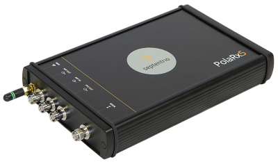
A new PolaRx5 Continuously Operating Reference Station (CORS) platform, offered by Septentrio Americas, is optimized for state departments of transportation (DOTs) and other real-time-kinematic (RTK) network operators.
The Septentrio PolaRx5 GNSS receiver.
The PolaRx5 CORS receivers can be purchased at special pricing by UNAVCO member organizations and affiliates. Septentrio has been selected by UNAVCO as the preferred vendor of CORS receivers under a multi-year agreement.
The PolaRx5 is powered by Septentrio’s AsteRx4 next-generation multi-frequency engine. It offers 544 hardware channels and supports all major satellite signals including GPS, GLONASS, Galileo and BeiDou, as well as regional satellite systems such as QZSS and IRNSS.
Septentrio’s Advanced Interference Mitigation (AIM+) technology enables the PolaRx5 to filter out both intentional and unintentional sources of radio interference, from narrowband signals over high-powered pulsed signals to chirp jammers and Iridium transmitters.
In addition, Septentrio’s patented APME+ multipath mitigation technology guarantees superior measurement quality by eliminating short-delay multipath errors without introduction of bias, the company said.
The PolaRx5 leverages Septentrio’s web interface and built-in Wi-Fi and Bluetooth interfaces to give users complete control and visibility of the receiver. The user interface integrates into existing network management systems. The web browser provides secure access to all receiver settings and status, data storage and firmware upgrades, as well as a built-in spectrum analyzer for system monitoring.
“The multi-constellation PolaRx5, with its powerful interference and multipath mitigation and new Web interface, is the ideal solution for DOTs to modernize their aging CORS installations to the newest GNSS technology,” said Neil Vancans, vice president of Septentrio Americas.
KVH Industries is developing a fiber optic gyro (FOG)-based, low-cost inertial sensor for self-driving cars.
The company also released a Developer’s Kit to assist design engineers with integrating FOG technology into driverless car control systems.
KVH’s high-precision FOG is key to a driverless car’s performance. In this photo, the red illumination represents light moving through the FOG’s optical circuit of coiled fiber; this circuit is the FOG’s sensing unit — it is mounted with power and processing electronics within a driverless car to provide precise data for the car’s navigation systems.
FOGs and FOG-based inertial measurement units (IMUs) are key parts of the sensor mechanisms that are essential for highly accurate autonomous car performance, KVH said. For example, FOGs provide precise azimuth measurements that an autonomous car’s logic processing unit and control systems need to determine motion through a curve.
An IMU — which includes FOGs and accelerometers in one compact package — also provides highly accurate 6-degrees-of-freedom angular rate and acceleration data to precisely track the position and orientation of the car even when GPS is unavailable, helping the car stay on course.
As a manufacturer of high-performance sensors and integrated inertial systems for defense and commercial guidance and stabilization applications, KVH Industries has experience in autonomous vehicle prototype programs and unmanned applications.
“Extremely precise heading based on fiber-optic gyro technology is absolutely essential for autonomous vehicle performance,” said Martin Kits van Heyningen, KVH’s chief executive officer. “This is something we learned from having been involved with more than a dozen driverless car development programs over the years.”
“What we are seeing now is that each driverless vehicle concept in development around the world is being designed in a unique way,” said Kits van Heyningen. “With so many different possibilities, developers can accelerate their progress by working with a proven technology such as KVH’s FOGs and FOG-based IMUs and leveraging our experience to ensure their success.”
Developer’s Kit. The new Developer’s Kit includes the user interface software and all components needed to connect a KVH FOG or FOG-based IMU to a computer to configure, analyze and test a unit. “The kit is designed to help engineers get up and running in minutes, making it easier to run diagnostics and accelerate their system development,” said Roger Ward, KVH’s director of FOG product development.
Driverless cars represent one of the fastest areas of autonomous-systems development. Transportation experts, automotive manufacturers and engineers alike predict that driverless cars will be commonplace soon.
An updated policy concerning automated vehicles will soon be published by the National Highway Traffic Safety Administration (NHTSA), which is part of the U.S. Department of Transportation. “The rapid development of emerging automation technologies means that partially and fully automated vehicles are nearing the point at which widespread deployment is feasible,” NHTSA said.
“We have successfully produced more than 90,000 fiber-optic gyros for an extensive range of unmanned applications, in part because of our ability to tailor size, performance, and cost to meet different design needs,” said Jeff Brunner, KVH’s vice president for FOG operations. “Controlling the entire FOG design and manufacturing process gives us that advantage, and makes it possible to produce a low-cost sensor when driverless cars enter full-scale production.”
KVH’s FOGs and FOG-based IMUs are in use in prototype programs not only for autonomous cars, but also for production programs for underwater unmanned vehicle navigation and rail/track geometry measurement systems, to name just a few.
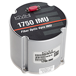
The KVH 1750 IMU.
In addition, KVH’s inertial products have been widely adopted for commercial applications such as land-based street mapping platforms, unmanned aerial systems, camera stabilization systems and remotely operated subsea systems.
As more and more programs and platforms use KVH’s inertial products, they are becoming the reference standards of the unmanned world. For example, KVH’s 1750 IMU was an integral part of 11 of the 23 humanoid robot finalists in last year’s DARPA Robotics finals, a competition designed to showcase robots capable of intervening for and even replacing humans in high-risk situations such as fires, earthquakes, and other natural disasters.
“Our IMUs and inertial sensors have already been used in a wide range of products and applications, and we know that it’s just the beginning,” said Kits van Heyningen. “We are thrilled to play a role in these exciting developments and emerging applications that are literally changing everyday life.”
Basic procedures and tools for ensuring GNSS-derived orthometric heights meet the project’s desired accuracy
To date, this series of columns has addressed the following topics: basic concepts of GNSS-derived heights, National Geodetic Survey’s (NGS) guidelines for establishing GNSS-derived ellipsoid heights (NGS 58), differences between hybrid and scientific geoid models, procedures and tools for detecting GNSS-derived ellipsoid height data outliers, and basic procedures for estimating GNSS-derived orthometric heights (NGS 59). These columns are meant to provide the reader with basic concepts, routines, and procedures for analyzing, evaluating, and estimating GNSS-derived heights.
As mentioned in the last column “Determining valid North American Vertical Datum of 1988 (NAVD 88) published heights is the most important process when using GNSS data and geoid models to estimate GNSS-derived orthometric heights.” In Part 5 (February 2016) of this series, we discussed NGS 59 guidelines and methods for evaluating the results of the GNSS project. It provided methods for evaluating the results of the project and identifying stations with valid NAVD 88 published heights. In this column, we will continue to analyze the changes in adjusted heights due to different height constraints and compare the results to the published NAVD 88 orthometric heights.
First, we need to discuss what should be considered an outlier when identifying valid NAVD 88 published heights to be used as constraints. According to NGS guidelines for performing GNSS adjustments, the rule of thumb for outliers are shifts greater than 2 cm horizontally and 4 cm vertically (see highlighted section in the box below). The guidelines also stated that “It is important to realize that this threshold is merely a ‘rule of thumb.’ For individual projects, unconstraining a station may be necessary if shifts are less than the ‘rule of thumb’ threshold, and in some cases it can remain constrained even if shifts slightly exceed the threshold.”
It is important to understand this concept because constraining the height of a station influences the heights of stations nearby that constraint. Also, not constraining a published height of a station will result in establishing a new height for that station which means it could be inconsistent with other published stations nearby that station. If the station had moved since the last time it was leveled to then not constraining the height is the appropriate action to take. However, if the shift is due to some other reason (such as a previous adjustment distribution correction, or ellipsoid and/or geoid issue), then constraining the height may be the appropriate action to take. Selecting constraints is not an exact science; as a matter of fact, at times, it appears to be more like an art or like solving an enigmatic puzzle.
Excerpt of NGS Adjustment Document, adjustment_guidelines.pdf, under section 5 titled Constrained Horizonal Adjustment.
As a general rule, if the adjusted values of the constrained coordinates of a station shift by more than 2 cm horizontally and/or 4 cm in height, its horizontal coordinates and/or ellipsoid height, respectively, should be unconstrained. Doing so means that the published values for the unconstrained passive control station will be updated by the adjusted values determined in the submitted survey (CORS coordinates will not be updated). This 2 cm horizontal and 4 cm vertical threshold is consistent with that used by NGS for updating published CORS coordinates, although for CORS this is done by NGS independent of individual campaign-style GPS projects. It is important to realize that this threshold is merely a “rule of thumb.” For individual projects, unconstraining a station may be necessary if shifts are less than the “rule of thumb” threshold, and in some cases it can remain constrained even if shifts slightly exceed the threshold. The decision to constrain or not constrain also depends on other factors, such as the statistics of the adjustment, residuals, shifts at other stations, and station accuracies. It requires judgment and should not simply be an automatic response to constrained station shifts.
The NGS guideline mentioned above is for horizontal coordinates and ellipsoid heights. The NGS guidelines under section 6 implies that the user should apply the same guidelines for shifts between GNSS-derived orthometric heights and published NAVD 88 orthometric heights (see highlighted section in the box below). The guidelines also recommend that the user analyze the shifts of stations near each other to determine if stations nearby each other are shifting consistently or if one of the station’s value appears to be an outlier (see underlined section in box below).
Excerpt of NGS Adjustment Document, adjustment_guidelines.pdf, under section 6 titled Vertical Adjustment (Free and Constrained).
SECTION 6, VERTICAL ADJUSTMENTS (FREE AND CONSTRAINED)
6-1. Create the vertical free Afile (Afilevf). Fix one position and one published orthometric height. They can be from the same station or different stations (e.g., good horizontal position in one CC record for a CORS, good OH in separate CC record for a bench mark). Leaving column 77 of the CC record blank indicates the record contains an orthometric height value. Standard deviations of the constrained coordinates and heights should NOT be entered (i.e., columns 15-32 of the CC record should be blank).
Include the VS record from the horizontal constrained Afile.
70-76 Height, units of millimeters (integer)
77-77 Height Code blank — orthometric height
6-2. Run Adjust with minimum constraints. Input: Bfileght, Afilevf, Gfile, Output: adjvf.out, Bfilevf
Assuming the adjustment ran to completion, the statistics of this run will be identical to those of the horizontal free adjustment. Check adjvf.out for big shifts between published and free-adjusted heights.
It would be helpful to compute the shifts between the results of the vertical free adjusted and the published heights. Additionally, plot these shifts on a project sketch to determine if several heights near each other are shifting consistently or a height appears to be an outlier and therefore should not be used as control. For inconsistent shifts use resources available such as recovery notes, photographs, and rubbings of the mark. Possible causes could include movement, an unintended mark was observed such as the underground mark instead of the surface mark, or occupying a reference mark rather than the parent station. Look for inconsistent shifts as opposed to areas where the shifts, even high shifts, are consistent. Likewise, look at the geoid heights to ensure they are consistent. If no cause for the shift can be found, the orthometric height may need to be readjusted.
6-3. Create the vertical constrained Afile (Afilevc). Constrain all previously adjusted orthometric heights as indicated above and one NAD 83 adjusted position. The same comments about CC records apply. All GPS-derived Ht Mod heights should be constrained along with bench marks. For ht mod stations the datasheet will read:
HT_MOD – This is a Height Modernization Survey Station.
Include the VS record with its appropriate values.
6- 4. Run Adjust with vertical constraints. Input: Bfilevf, Afilevc, Gfile, Output: adjvc.out, Bfilevc
Run PrePlt2 to list and sort the residuals. Investigate observations with large shifts or residuals to see if any heights should be readjusted. Apply the same rule as in the horizontal constrained adjustment: no rejections due to constraints. Free any heights in question and rerun as a test. Note the differences between the published and readjusted heights obtained from the vertical constrained adjustment. Consider the requirements of the project before deciding whether to readjust additional points. Save the output Bfile from the final constrained vertical adjustment.
In Part 5, I highlighted a potential issue at station Phaniel. I’ve included the diagrams and tables from Part 5 that depicts the differences between GNSS-derived orthometric heights from a minimum-constraint adjusyment (using GEOID12B and xGeoid15b) and the published NAVD 88 height values (see figures 1-4, and tables 1-2). Looking at figures 1 and 2, there are several large differences between closely spaced constraints when using the hybrid geoid model – Phaniel, Buffalos 2, V 49, and Row 9. As stated in Part 2, the user should compute the results using both the hybrid and the scientific geoid models. Figures 3 and 4 depict the differences using the scientific geoid model xGeoid15b. Notice that the large differences between Phaniel and Buffalo 2 decreased from 4.9 cm using GEOID12B to 0.7 cm using xGeoid15b. However, the larger relative difference between Phaniel and V 49 (3.8 cm) and ROW 9 (5.2 cm) still exists. Also, the difference between Buffalo 2 and V 49 is large (3.1 cm), and Buffalo 2 to Row 9 is large (4.5 cm), but the difference between V 49 and Row 9 is less than 2 cm. The neighbor stations of Row 9 all seem to agree within a couple of centimeters indicating that Buffalo 2 may be a station that needs further investigation.
Figure 1. [Figure 3 from Part 5] Diagram depicting differences between GNSS-derived orthometric heights from a Minimum-Constraint Adjustment (using GEOID12B) and published NAVD 88 height values (units=cm).Figure 2. [Figure 4 from Part 5] Diagram depicting differences between GNSS-derived orthometric heights from a Minimum-Constraint Adjustment (using GEOID12B) and published NAVD 88 height values (units=cm).
Figure 3. [Figure 5 from Part 5] Diagram depicting differences between GNSS-derived orthometric heights from a Minimum-Constraint Adjustment (using xGeoid15b) and published NAVD 88 height values (units=cm).Figure 4. [Figure 6 from Part 5] Diagram depicting differences between GNSS-derived orthometric heights from a Minimum-Constraint Adjustment (using xGeoid15b) and published NAVD 88 height values (units=cm).
Next we need to look at the adjusted ellipsoid heights from a minimum-constraint solution compared to the published ellipsoid heights. This procedure was decribed and demonstrated in Part 4. Figure 5 is plot of adjusted ellipsoid height minus published NAD 83 (2011) ellipsoid heights for stations near Phaniel. Figure 5 indicates that the adjusted ellipsoid heights at Buffalo 2, Phaniel, and V 49 all agree within 2 cm. As a matter of fact, Buffalo 2 and Phaniel agree to better than 1 cm from the NAD 83 (2011) published heights. This is an indication that the orthometric height of station Phaniel may be an outlier and should not be constrained. The leveling network in the area requires investigation to validate this conclusion. This will be addressed in a future column. Looking at Tables 1 and 2, two other stations, stations Plaza and Row 3, have large differences between the GNSS-derived orthometric heights from a minimum-constraint adjustment and the published NAVD 88 heights, and they should be investigated.
Figure 5. Plot of adjusted ellipsoid height minus published NAD 83 (2011) Ellipsoid Heights for Stations near Phaniel (the number is the difference for that particular station; units = cm).Table 1. Differences between GNSS-derived orthometric heights from a minimum-constraint adjustment (using GEOID12B) and published NAVD 88 heights (GEOID12B results sorted and highlighted).Table 2. Differences between GNSS-derived orthometric heights from a minimum-constraint adjustment (using xGeoid15b) and published NAVD 88 heights (xGeoid15b results sorted and highlighted).
Figure 6 is a diagram depicting differences between GNSS-derived orthometric heights from a minimum-constraint adjustment using GEOID12B and published NAVD 88 heights surrounding station Plaza. The user should notice that the relative difference in height changes between Plaza and 37 DRD is -3.8 cm (-2.5 – 1.3) and between Plaza and Fifth it is -3.2 cm (-2.5 – 0.7). This is an indication that there is a potential issue with station Plaza. Next, we need to compute the results using xGeoid15b. Figure 7 is a plot of the differences surrounding station Plaza using xGeoid15b. Figure 7 shows that station Plaza outliers relative to station 37 DRD and Fifth are exactly the same, i.e., -3.8 cm (-3.2 – 0.6) and -3.2 cm (-3.2 – 0.0) respectively. Something interesting to note is that station J 181 difference decreased from 2.1 cm using GEOID12B (see figure 6) to 1.1 cm using xGeoid15b (see figure 7). Once again, this is a reason why users should use both the hybrid geoid model and the scientific geoid model when analyzing GNSS-derived orthometric heights.
Figure 6. (More Detail at Station Plaza) Diagram depicting differences between GNSS-derived orthometric heights from a Minimum-Constraint Adjustment (using GEOID12B) and published NAVD 88 height values (units=cm).
Figure 7. (More Detail at Station Plaza) Diagram depicting differences between GNSS-derived orthometric heights from a Minimum-Constraint Adjustment (using xGeoid15b) and published NAVD 88 height values (units=cm).
The other station to investigate based on the large difference in table 2 is station Row 3. Figure 8 is a diagram depicting the differences near station Row 3 using GEOID12B. Notice that the difference at Row 3 is considerably less than the 4 cm; however, the relative difference between Row 3 (-2.7 cm) and station 384 JAS (0.2 cm) is -2.9 cm. This doesn’t seem too large but computing the results using xGeoid15b indicates something different. Figure 9 is a plot of the differences using the scientific geoid model xGeoid15b. Notice that the difference at station Row 3 increased to -3.8 cm and the relative difference between Row 3 and 384 JAS is -3.9 cm. Note, this again emphases the importance of using both the hybrid and scientific geoid models when analyzing GNSS-derived orthometric heights. This large relative difference is an indication that the height of station Row 3 may not have a valid NAVD 88 published height and should be further investigated before constraining the height in the final adjustment.
Figure 8. (More Detail at Station Row 3) Diagram depicting differences between GNSS-derived orthometric heights from a Minimum-Constraint Adjustment (using GEOID12B) and published NAVD 88 height values (units=cm).Figure 9. (More Detail at Station Row 3) Diagram depicting differences between GNSS-derived orthometric heights from a Minimum-Constraint Adjustment (using xGeoid15b) and published NAVD 88 height values (units=cm).
After analyzing the differences between GNSS-derived orthometric heights from a minimum-constraint adjustment and published NAVD 88 heights to help identify potential outliers, the user can perform a constrained adjustment holding the published height values as constraints. The user should ensure that a constraint does not significantly affect the adjusted heights of neighboring stations. To understand the effects of the constraints on the heights of stations that are not constrained, the user can plot the changes in adjusted heights between the constrained adjustment and the minimum-constraint adjusted heights (with a bias removed). As mentioned in Part 5, any constraint can be used to obtain a minimum-constraint solution so removing a bias based on the differences between the published height values and the adjusted height values obtained from a solution constraining one published height is appropriate. Figure 10 is a plot that depicts the differences between the adjusted heights from an adjustment with all published NAVD 88 height values constrained and the adjusted heights values from the minimum-constraint adjustment. Figure 10 highlights the large relative changes of closely spaced stations such as between Phaniel (-2.8 cm) and Open (-0.6 cm). This means that the constraint at station Phaniel has changed the relative height difference between station Phaniel and station Open by 2.2 cm. This is a large change when you trying to obtain 2 cm heights. Another method to see the effect of the constraints is by plotting the changes in “dU” residuals between the constrained adjustment and the minimum-constraint adjustment. Figure 11 is a plot of the differences in vector “dU” residuals between the constrained adjustment (with all published heights constrained) and the minimum-constraint adjustment.
Figure 10. Diagram depicting differences between GNSS-derived orthometric heights from a Constrained Adjustment (All Published Heights Constrained) minus Minimum-Constraint Adjustment (using GEOID12B) – units=cm.
Looking at figure 11, the user can quickly see that constraining station Phaniel has changed the three vectors associated with Phaniel by 1.9 cm, 2.1 cm, and 2.3 cm. This means that the observed vectors were changed by 2 cm to be consistent with the constraint at Phaniel. This could have an impact on a surveyor performing leveling between these two stations. The analyst should now perform an adjustment not constraining the stations identified as potential outliers. At this moment, in this study, stations Phaniel, Plaza, and Row 3 are considered questionable and their heights will not be constrained.
Figure 11. Diagram depicting differences between dU Residuals of Vectors from a Constrained Adjustment (All Published Heights Constrained) minus Minimum-Constraint Adjustment (using GEOID12B) – units=cm.
Figure 12 is a diagram depicting the differences between the GNSS-derived orthometric heights from a constrained adjustment were the height values of stations Phaniel, Plaza, and Row 3 were not constrained. Figure 13 is a diagram depicting the differences between the dU residuals of baselines from the constrained adjustment with heights of stations Phaniel, Plaza, and Row 3 not constrained and the dU residuals from the minimum-constraint adjustment. Figures 14 and 15 provide more detail of the changes in residuals near station Phaniel. Figure 14 depicts the differences when all NAVD 88 heights are constrained and figure 15 depicts the differences when the suspected stations (Phaniel, Plaza, and Row 3) are not constrained. Comparing figures 14 and 15 clearly show that by constraining station Phaniel, the relative differences between station Phaniel and its neighbors are adversely effected by the constraint. For example, the difference in dU residuals between Phaniel and Brown Az Mk decreased from 2.3 cm to -0.2 cm resulting in a 2.5 cm relative height change.
Figure 12. Diagram depicting differences between GNSS-derived orthometric heights from a Constrained Adjustment (Three Stations Unconstrained) minus Minimum-Constraint Adjustment (using GEOID12B) – units=cm.Figure 13. Diagram depicting differences between dU Residuals of Vectors from a Constrained Adjustment (Three Stations Unconstrained) minus Minimum-Constraint Adjustment (using GEOID12B) – units=cm.Figure 14. (More Detail at Station Phaniel) Diagram depicting differences between dU Residuals of Vectors from a Constrained Adjustment (All Stations Constrained) minus Minimum-Constraint Adjustment (using GEOID12B) – units=cm.Figure 15. (More Detail at Station Phaniel) Diagram depicting differences between dU Residuals of Vectors from a Constrained Adjustment (Three Stations Unconstrained) minus Minimum-Constraint Adjustment (using GEOID12B) – units=cm.
As previously mentioned, station Plaza is another station with a large difference between the adjusted height from the minimum-constraint adjustment and its published height (see tables 1 and 2). Constraining station Plaza results in very large dU residuals between station Plaza and station 37 DRD, i.e, 3.7 cm over a distance of 1.1 km (see figure 16). By not constraining the height of station Plaza the dU residuals on the vector between station Plaza and station 37 DRD changed from 3.7 cm to 0.4 cm (see figure 17). Also, the dU residuals on the vector between station College and station Hudson changed from -1.8 cm to -0.1 cm, and dU residuals on the vector between station Dorsett and station Hudson changed from -1.7 cm to 0.2 cm. The distance between Dorsett and Hudson is 1.2 km. The allowable section closure for second-order, class 2 leveling in 1.2 km is 0.88 cm. If a user wanted to check their leveling work using these two stations they may not check within the allowable because of the large distribution correction applied to the adjusted heights due to constraining the height of station Plaza.
Figure 16. (More Detail at Station Plaza) Diagram depicting differences between dU Residuals of Vectors from a Constrained Adjustment (All Stations Constrained) minus Minimum-Constraint Adjustment (using GEOID12B) – units=cm.Figure 17. (More Detail at Station Plaza) Diagram depicting differences between dU Residuals of Vectors from a Constrained Adjustment (Three Stations Unconstrained) minus Minimum-Constraint Adjustment (using GEOID12B) – units=cm.
Next, the user should look at the differences in ellipsoid heights between minimum-constraint adjustment and published NAD 83 (2011) ellipsoid heights in the area of station Plaza (see figure 18). Station Plaza did not have a published NAD 83 (2011) ellipsoid height but the closest two stations (Dorsett and Salisbury CORS ARP) both agree within 0.6 cm of the published NAD 83 (2011) ellipsoid heights. This is a good sign tht the ellipsoid heights meet the desired accuracy but doesn’t help to explain the large difference at station Plaza.
Figure 18. (More Detail at Station Plaza) Diagram depicting differences between Adjusted GNSS-Derived Ellipsoid Heights (with average bias removed) minus Published NAD 83 (2011) Ellipsoid Heights (units=cm).
The third station with a large relative difference highlighted in table 2 is station Row 3. Figures 19 and 20 provide more detail of the changes in residuals near station Row 3. Notice that the dU residual of the vector between station Railroad and Magna changed from 1.5 cm to 0.1 cm when the height of Row 3 is not constrained. The distance between the two stations is 4 km so the effect of constraining this station is not really significant. It should be noted that one of the reasons it’s being investigated is because of the large relative difference between Row 3 and station 384 JAS using xGeoid15b (-3.9 cm, see figure 9). Figure 21 is a plot of the differences in ellipsoid heights obtained from the minimum-constraint adjustment and their published NAD 83 (2011) ellipsoid heights in the vicinity of station Row 3. Station Row 3 does not have a published NAD 83 (2011) ellipsoid height but all of the stations surrounding the station are less than 2 cm. There does not appear to be any large outliers compared with the published ellipsoid heights in the area. Once again, this means that the next step in the process is to investigate the leveling network in the area.
Figure 19. (More Detail at Station Row 3) Diagram depicting differences between dU Residuals of Vectors from a Constrained Adjustment (All Stations Constrained) minus Minimum-Constraint Adjustment (using GEOID12B) – units=cm.Figure 20. More Detail at Station Row 3) Diagram depicting differences between dU Residuals of Vectors from a Constrained Adjustment (Three Stations Unconstrained) minus Minimum-Constraint Adjustment (using GEOID12B) – units=cm.Figure 21. (More Detail at Station Row 3) Diagram depicting differences between Adjusted GNSS-Derived Ellipsoid Heights (with average bias removed) minus Published NAD 83 (2011) Ellipsoid Heights (units=cm).
Up to this point we have analyzed changes in adjusted heights due to different constraints and compared the results to the published NAVD 88 GNSS-derived orthometric heights to identity stations that should be constrained in the final adjustment. As one can see, performing GNSS-derived orthometric height adjustments is more like an art than an exact science. There are a lot of variables and unknowns. Every constraint has an influence on the final set of adjusted heights. Determining this effect and the consequences of selecting an invalid constraint has been described in this column.
When incorporating new geodetic data into the National Spatial Reference System, it is important to maintain consistency between neighboring stations. If the published height of a station is not constrained, it will be superseded by the newly adjusted height. If the station has moved since the last time its height was established then superseding the height is the appropriate action to take. If the difference is due to some other reason such as the results of a previous adjustment distribution correction then superseding the height may not be the appropriate action to take.
In my next column, Part 7, we will look at the design of the NAVD 88 leveling network and published heights in the area to help determine the final set of stations to constrain.


![Figure 1. [Figure 3 from Part 5] - Diagram depicting differences between GNSS-derived orthometric heights from a Minimum-Constraint Adjustment (using GEOID12B) and published NAVD 88 height values (units=cm).](https://stage.globalpositioningnews.com/wp-content/uploads/2016/04/Rowan-County_Newsletter_5_3.jpg)
![Figure 2. [Figure 4 from Part 5] - Diagram depicting differences between GNSS-derived orthometric heights from a Minimum-Constraint Adjustment (using GEOID12B) and published NAVD 88 height values (units=cm).](https://stage.globalpositioningnews.com/wp-content/uploads/2016/04/Rowan-County_Newsletter_5_4.jpg)
![Figure 3. [Figure 5 from Part 5] - Diagram depicting differences between GNSS-derived orthometric heights from a Minimum-Constraint Adjustment (using xGeoid15b) and published NAVD 88 height values (units=cm).](https://stage.globalpositioningnews.com/wp-content/uploads/2016/04/Rowan-County_Newsletter_5_5.jpg)
![Figure 4. [Figure 6 from Part 5] - Diagram depicting differences between GNSS-derived orthometric heights from a Minimum-Constraint Adjustment (using xGeoid15b) and published NAVD 88 height values (units=cm).](https://stage.globalpositioningnews.com/wp-content/uploads/2016/04/Rowan-County_Newsletter_5_6.jpg)


