Category: Research & Development

  • Innovation: Navigation from LEO

    Innovation: Navigation from LEO

    Current Capability and Future Promise

    GPS signals are so weak, they cannot be used reliably where they are obstructed such as indoors or in concrete canyons. But if the satellites were much closer, their signals would be much stronger. The low Earth orbit Iridium constellation is already orbiting and providing a PNT service. This month we learn about its current capability and future promise.

    By David Lawrence, H. Stewart Cobb, Greg Gutt, Michael O’Connor, Tyler G.R. Reid, Todd Walter and David Whelan

    (A shortened version of “Innovation Insights” appeared in the magazine.)

    INNOVATION INSIGHTS with Richard Langley

    WHOA CANADA! July 1st marks Canada’s sesquicentennial. In 1867, four Canadian provinces, Ontario and Quebec (up to then known as the single Province of Canada), Nova Scotia and New Brunswick, joined together to form The Dominion of Canada — the name suggested by New Brunswick’s Sir Leonard Tilley. Other provinces came on board later with the last, Newfoundland and Labrador, joining in 1949.

    Apart from my interest in educating all and sundry about the origins of the “true north, strong and free,” what has this got to do with GNSS or allied technologies? Well, it turns out that Canada has played and continues to play an important role in the development of communications and navigation technologies.

    It started on Christmas Eve, 1906, when Canadian inventor Reginald Fessenden carried out the first amplitude modulation radio broadcast of voice and music. And in 1925, Edward “Ted” Rogers, a Canadian pioneer in the radio industry, invented a radio tube using alternating current that became a worldwide standard in radio circuits.

    Many other developments in terrestrial communications took place in Canada over the years including microwave repeater technology and shortwave radio broadcasting from the famed transmitter plant (now defunct, unfortunately) established near Sackville, New Brunswick, during World War II.

    There have also been significant Canadian advances in satellite technology. The first Canadian satellite, Alouette (French for “skylark”), was launched in September 1962 to study the ionosphere. Launched by the United States, it was the first satellite to be constructed by a country other than the U.S. or the Soviet Union. Several other Canadian ionospheric research satellites have been orbited since including CAScade, Smallsat and IOnospheric Polar Explorer or CASSIOPE, launched in September 2013. CASSIOPE carries eight instruments for studying the ionosphere including the University of New Brunswick’s GPS Attitude, Positioning, and Profiling instrument.

    Canada has also been a leader in satellite communications technology. The first Anik geostationary satellite was launched in November 1972. (Anik means “little brother” in Inuktitut.) Eight more Anik satellites were launched subsequently including Anik F1R, which is also used to broadcast Wide Area Augmentation System information to GPS receivers. And the first satellite to explore the 14/12-GHz band for direct broadcasting to homes and businesses was Canada’s Communications Technology Satellite, dubbed Hermes, launched in January 1976.

    And, of course, we don’t need to mention the Remote Manipulator System on the International Space Station, commonly known as Canadarm, nor the work of celebrity Canadian astronaut Col. Chris Hadfield.

    In the area of satellite navigation, Canada is known for its development of techniques to use the U.S. Navy Navigation Satellite System or Transit for one-meter positioning accuracy permitting establishment of geodetic control points such as in Canada’s far north. Canada was also an early adopter of GPS and with software and hardware developments by industry, government and academia has made its mark in the world of precision positioning, navigation and timing.

    Another Canadian initiative is the Aerion satellite-based air traffic surveillance system that will use the enhanced low Earth orbit Iridium constellation.

    And we shouldn’t forget that Canada is slated to provide the search and rescue package for the GPS III satellites.

    Speaking of GPS, we all know what a great technology it is, providing the “gold standard” in global satellite navigation. But it does have one dominant problem: the weakness of the signals. The signals are so weak that they cannot be used reliably where they are obstructed such as indoors or in concrete canyons. The problem stems from the fact that these medium Earth orbit satellites are far away and their energy is significantly spread out during their passage to Earth. If the satellites were much closer to the Earth, their signals would be much stronger. Mind you, you would need more satellites to provide global coverage. Fantasy? No. There is already a constellation of satellites in orbit providing such a PNT service. It is Iridium–the same constellation that will provide the Canadian-initiated aircraft tracking system–and in this month’s column we will learn about is current capability and future promise. Pretty neat, eh?


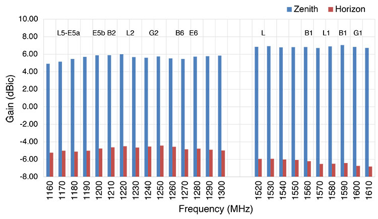
    With the advent of smartphones, there are now more than four billion devices that make use of GNSS. These satellite navigation systems provide not just the blue dot representing location on our phones, but also support the critical infrastructure we rely upon.

    The U.S. Department of Homeland Security recognizes that all 16 sectors of U.S. critical infrastructure depend on GPS — 13 of which have critical dependence. A recent report by London Economics estimates the cost of a GNSS outage to the U.K. alone would be over £1B per day.With autonomous systems on the rise, our reliance on GNSS will only be increasing.

    As we become more dependent on this technology, we become vulnerable to its limitations. One major shortcoming is signal strength. Designed to work in an open-sky environment, GNSS is severely limited in deep attenuation environments, with little or no service in dense cities or indoors. Furthermore, we are susceptible to jamming where a 20-watt GNSS jammer can deny service over a city block.

    The proximity of low Earth orbit (LEO) has the potential to provide much stronger signals than the distant GNSS core-constellations like GPS in medium Earth orbit (MEO). Today, the only LEO system with global coverage is the Iridium constellation used primarily for communications.

    FIGURE 1 shows the 31-satellite GPS constellation in contrast with the 66-satellite Iridium network. The scale of the difference in distance (several Earth radii) is extraordinary. The result is that Iridium signals are 300 to 2,400 times stronger than GNSS signals on the ground, making them attractive for use in position, navigation and timing (PNT) applications where GNSS signals are obstructed.

    FIGURE 1. The 66-satellite Iridium constellation in low Earth orbit and 31-satellite GPS constellation in medium Earth orbit.

    LEO-based PNT is now mainstream, in the form of real-time signals that have been delivered over the Iridium satellite network since May 2016. This service is made possible by Satelles in partnership with Iridium Communications Inc. in a service called Satellite Time and Location (STL), a non-GNSS solution for assured time and location that is highly resilient and physically secure. Consumers, businesses and governments are already using these LEO-based signals in environments with high GNSS interference or occlusion.

    The security features of these signals are also used to reliably validate GNSS PNT solutions in real time to help mitigate potential spoofing. Furthermore, the fast LEO orbits of Iridium generate Doppler-frequency-shift signatures significantly stronger than GPS, increasing the utility of the STL signal for positioning applications.

    STL field tests demonstrate a positioning accuracy of 20 meters and timekeeping to within 1 microsecond, all in deep attenuation environments indoors. This adds substantial robustness in augmenting the GNSS core constellations like GPS and also allows for a standalone backup in many applications.

    LEO Constellations: Past, Present, Future

    In 1964, Transit (or the U.S. Navy Navigation Satellite System) became the first operational satellite navigation system. This constellation typically consisted of five to 10 satellites placed in polar orbits with an altitude of about 1,100 kilometers. Unlike many terrestrial radio navigation systems, a position fix was not instantaneous. It required 10 to 16 minutes of observation as a satellite passed overhead to achieve the needed geometric diversity. There was also latency; users had to wait for a satellite to come into view, which could take from 30 to 100 minutes.

    The trade-off was accuracy; early performance was a few hundred meters and was later improved to 20 meters (and even down to about 1 meter for multiple-pass fixed-site surveys), the best performance of its day. In 1967, Transit became open for civilian use and remained operational until 1996 when GPS was at full operational capability.

    The Soviet Union developed a system similar to Transit known as Parus/Tsikada, with first satellites on orbit in 1967. Parus/Tsikada operated on the same passive Doppler observation principle as Transit, on similar frequencies and in similar polar orbits.

    Today, the largest satellite constellation with constant global coverage is Iridium. With 66 LEO satellites delivering worldwide satellite connectivity, including the poles, this system has tenfold more satellites than Transit had. Along with its strong signals compared to the GNSS core-constellations in MEO, Iridium’s global coverage makes it ideal for use in PNT applications where GNSS is obstructed.

    Figure 1 shows the scale of the difference in altitude with Iridium at 780 kilometers and GPS at 20,200 kilometers. This has substantial implications not only for signal strength, but also for coverage.

    Though Iridium has twice as many satellites as GPS, at the Equator users can often only see one satellite at a time, whereas they can see 10 from GPS. This was one of the fundamental trades considered in the design of the GPS constellation. The higher the altitude, the more each launch cost; the lower, the more satellites had to be built to provide coverage. To put this in perspective, global coverage for one satellite in view at all times requires fewer than 10 satellites in MEO, but requires closer to 100 in LEO.

    Future LEO Constellations

    The hundreds of LEO satellites needed to match the coverage of GPS may be coming. In late 2014 and early 2015, the International Telecommunication Union reported a half-dozen filings for spectrum allocation for large constellations of LEO satellites.

    In January 2015, OneWeb announced a partnership with Virgin and Qualcomm to produce a constellation of 648 LEO satellites to deliver broadband Internet globally. This represents the next order of magnitude, with tenfold more satellites than Iridium.

    Within days of this announcement, SpaceX, with support from Google, announced a similar ambition for a constellation of more than 4,000 LEO satellites.

    In August 2015, Samsung expressed interest with a proposal for a LEO constellation of 4,600. Boeing joined the race in June 2016, announcing plans for a LEO constellation of nearly 3,000 satellites.

    These LEO constellations are being proposed to keep up with the rising demand for broadband, not to replace ground infrastructure, and will provide Internet access to the 54% of the global population that lack that access.

    TABLE 1 compares the GNSS core constellations in MEO to the big (Iridium), broadband (OneWeb, SpaceX, Boeing) and early navigation (Transit, Parus/Tsikada) LEO constellations.

    TABLE 1. Constellation comparison.

    LEO versus MEO

    Low and medium Earth orbit each have their individual strengths and weaknesses in the context of navigation as summarized by TABLE 2.

    TABLE 2. Comparison of LEO and MEO systems for navigation.

    Closer to Earth, LEO offers less spreading loss and improved signal strength on the ground. FIGURE 2 shows that the signal spreading (or space) loss for Iridium is between –140 and –130 dB compared to GPS at –160 dB.

    This stems from Iridium being 25 times closer to Earth than GPS, resulting in a gain in the neighborhood of 252, which is approximately 30 dB (1,000 fold). This is confirmed by field tests where the carrier-to-noise-density ratio (C/N0) is typically 45 dB-Hz for GPS but closer to 80 dB-Hz for Iridium.

    FIGURE 2. Slant range and spreading loss as a function of orbital altitude and user elevation angle (GSO = geostationary orbit).

    Now, we face the drawback of LEO proximity: coverage. Being closer to Earth means that satellites have much smaller footprints as shown in FIGURE 3.

    FIGURE 3. Comparison of medium and low Earth orbit satellite distance and footprints (drawn to scale).

    FIGURE 4 shows the satellite-footprint radius as a function of orbital altitude and user elevation mask angle. This plot shows the GPS footprint to be threefold larger than Iridium’s, corresponding to nine times more area covered. Hence, to achieve the same coverage as GPS with Iridium’s altitude, a LEO constellation requires an order of magnitude more satellites.

    FIGURE 4. Satellite footprint radius as a function of orbital altitude and elevation angle (GSO = geostationary orbit).

    Another major difference between LEO and MEO is speed. A GPS satellite completes one Earth revolution every 12 hours, while Iridium does so in only 100 minutes. The shorter the orbital period, the faster the angular rate (also called mean motion) and the more quickly satellites pass overhead. The Earth-centered angular rate of Iridium is seven times faster than GPS.

    As a result, users on Earth’s surface see LEO Iridium satellites traverse the local sky in just over 10 minutes compared to hours with satellites in MEO. This characteristic gives rapid changes in geometry and several benefits for navigation.

    The swift motion whitens multipath (making it more random, like white noise) as reflections are no longer effectively static over short averaging times. Geometric diversity also leads to effective Doppler positioning as was once leveraged by Transit and now by STL using Iridium. Geometric diversity is also desirable for carrier-phase differential GNSS, allowing for much more rapid resolution of integer cycle ambiguities.

    Iridium-Satelles STL Service

    As previously mentioned, the STL service has been in operation since May 2016. Many from industry and government are already using this service to achieve a more robust PNT solution. This service will only continue to improve with the Iridium NEXT satellites under deployment — the first 10 were successfully launched in January.

    STL is a non-GNSS solution for assured time and location that is highly resilient and physically secure. STL utilizes the Iridium constellation to transmit specially structured time and location broadcasts. Due to their high RF power and signal-coding gain, the STL broadcasts are able to penetrate into difficult attenuation environments, including deep indoors. Like GNSS signals, these broadcasts are specifically designed to allow an STL receiver to obtain precise time and frequency measurements to derive its PNT solutions.

    STL is able to augment or serve as a back-up to existing GNSS PNT solutions by providing secure measurements in the presence of high attenuation (deep indoors), active jamming and malicious spoofing. Unlike the MEO GNSS satellites, Iridium uses 48 spot beams to focus its transmissions on a relatively small geographic area. The complex overlapping spot beams of Iridium combined with randomized broadcasts give a unique mechanism to provide location-based authentication that is extremely difficult to spoof.

    Two main technical innovations are applied to the existing Iridium quadrature phase-shift keying (QPSK) transmission scheme to facilitate precision measurements. First, the QPSK data at the beginning of an STL burst is manipulated to form a continuous wave (cw) marker, which can be used for burst detection and coarse measurement. Second, the remaining QPSK data in the burst is organized into pseudorandom sequences, reducing the effective information data rate while providing a mechanism for precise measurement via correlation with locally generated sequences.

    The processing gain of the sequence correlation operation also enhances the capability of the STL signal to penetrate buildings and other occlusions. STL is designed such that a receiver can reliably decode the bursts and perform precise Doppler and range measurements at attenuations of up to 39 dB relative to unobstructed reception. This is sufficient to penetrate buildings and other occlusions, providing coverage in most deep indoor and urban canyon environments.

    In environments where both GNSS and STL time and location fixes are available, the GNSS fixes will generally be more accurate. The key advantage of STL is its ability to provide time and position fixes where GNSS is not available because of occlusions, spoofing or other reasons. In this respect, GNSS and STL can be seen as complementary technologies, and it is apparent that receivers supporting both are highly desirable when practical. An example of a combined GNSS + STL receiver board is shown in FIGURE 5 and is available from Satelles.

    FIGURE 5. Custom STL receiver board capable of GNSS + Iridium operation.

    Signals in Challenging Environments

    To test the signal penetration of STL, trials of the system were undertaken at multiple locations inside an urban high-rise building. For these tests, locations with little or no GPS reception were chosen to measure the impact of such an environment on STL signal reception.

    Two GPS receivers were used, a smartphone with assisted GPS and a standalone consumer receiver using Bluetooth communications without assistance data. Similarly, STL was used with and without assistance. For these tests, STL assistance included real-time, out-of-band delivery of satellite clock and orbit data and message payload contents. These test locations ranged from the top (13th) to the bottom (2nd) floor as shown in FIGURE 6.

    FIGURE 6. Iridium-based STL test locations. These are indoor and deep attenuation environments where GPS is unavailable.

    The results show that only upper floors near windows were able to track at most one to two GPS satellites while lower floors could see none. STL, on the other hand, always experienced strong signals. Even on the lowest floor, with many layers of steel and concrete between the antenna and the sky, the C/N0 from Iridium was between 35 and 55 dB-Hz. GPS, by comparison, is typically between 35 and 50 dB-Hz in an open sky environment.

    Indoor Time-Transfer Capability

    To evaluate the timing performance of STL in a static, indoor environment, a custom STL receiver board was configured to generate a pulse-per-second (PPS) output. The difference in timing between the STL PPS was then compared to the timing output of a GNSS “truth” reference — in this case, a timing receiver that has nominal timing performance at least an order of magnitude better than the STL-based timing we were attempting to measure.

    FIGURE 7 shows the timing difference between the PPS signals generated by the STL receiver and the GNSS receiver, showing the STL ability to provide sub-microsecond timekeeping even in a deep attenuation environment.

    FIGURE 7. Iridium-based STL timekeeping results based on data from a 30-day indoor trial. This compares indoor STL timing with a GPS feed from outdoors. This shows STL’s timekeeping to be within 1 microsecond in a deep attenuation environment.

    While sub-microsecond timing is sufficient for many applications, higher timing accuracy is desired by some. It has been further demonstrated that STL is capable of achieving sub-100-nanosecond timekeeping in a stand-alone configuration with a rubidium-based STL receiver with an unknown static location indoors.

    Indoor Positioning Performance

    Unlike the time-transfer capability of STL, positioning requires satellite motion over time to achieve a reasonable 4D time-and-location fix. Therefore, understanding the convergence properties of STL positioning accuracy over time is important to understanding the applicability of STL for various potential uses.

    To study these convergence properties, STL data was collected over a 24-hour period in a one-story office environment. The data was then post-processed in a series of trials that each represented a different starting time in the data set — each trial offset to begin 5 seconds ahead of the previous trial’s start time. In this way, the 24-hour data set could be used to generate a statistically significant set of trial runs in which positioning convergence characteristics could be evaluated.

    We found out from the results of the post-processed trials that after 10 minutes of convergence, the STL solution had converged to an accuracy of better than 35 meters for 67% of the trials. After sufficient time, typically an accuracy of 20 meters can be achieved in deep attenuation environments such as indoors. The vertical accuracy of STL, in the absence of other measurements or vertical constraints, is comparable to the horizontal accuracy.

    Looking Forward

    We see the benefit of LEO in navigation with the operational STL using Iridium, where stronger signals allow for operation deep indoors and in other GNSS-challenged environments. Though extremely valuable as a complement to GPS, Iridium lacks the numbers to fully replace GPS as a standalone navigation system in all capacities as only one satellite at a time is typically in view.

    However, these numbers may be coming in LEO with the unprecedented scale of the recently announced Broadband constellations of OneWeb, SpaceX, Boeing and others summarized in Table 1. OneWeb’s constellation is nearly as large as the total number of operational satellites in LEO today and is an order of magnitude larger than Iridium. SpaceX’s and Boeing’s proposed constellations each have more than twice the total number of operational satellites in orbit in 2017.

    The unparalleled number of satellites in these proposed broadband LEO constellations gives rise to better geometry than any of the GNSS core-constellations in MEO by at least threefold, as shown by FIGURE 8.

    FIGURE 8. Comparison of geometric dilution of precision (98th percentile) as a function of constellation size and altitude (MEO = medium Earth orbit; GSO = geostationary orbit).

    This plot represents the 98th percentile geometric dilution of precision a user would experience on Earth as a function of constellation size and altitude, assuming a 5-degree elevation mask angle. This stronger geometry allows for relaxation of the signal-in-space user range error, while still matching the user position accuracy of GPS. This enables the use of lower than traditional cost satellite clocks and more amenable orbit determination levels.

    When combined with the more benign LEO radiation environment compared to MEO, satellite navigation payloads could be built using commercial off-the-shelf components in place of specialized space-hardened ones, greatly reducing cost. By partnering with these LEO constellation providers, much like Satelles has done with Iridium, a PNT service comparable to GPS could be achieved though with the added benefits of LEO including stronger signals and rapid changes in geometry.

    Conclusion

    Robust PNT services from LEO are here today, providing augmentation to GPS where GPS isn’t available. The addition of navigation signals from LEO provides a number of benefits. The faster LEO motion provides geometric diversity, giving rise to multipath whitening, faster initialization times for carrier-phase differential GNSS, and Doppler-based positioning.

    Perhaps most importantly, LEO constellations have the advantage of being closer to the Earth than the GNSS core constellations in MEO, experiencing less path loss and delivering signals 1,000 times (30-dB) stronger. This makes them more resilient to jamming and more capable in deep attenuation environments such as in urban canyons and indoors.

    This extra power allows the LEO-based Satelles STL using Iridium to achieve timekeeping within 1 microsecond and a positioning accuracy of 20 meters, all while deep indoors where GNSS is unavailable. This adds indispensable resilience and security to GNSS that we are increasingly reliant upon, creating a comprehensive satellite navigation system that truly works everywhere.

    This PNT service using Iridium is perhaps a sign of things to come. We’ve seen a progression in LEO use since the dawn of the Space Age, namely, an order of magnitude increase in constellation size every 30 years. Transit first offered an occasional position update based on a constellation of six satellites in the 1960s.

    Built in the 1990s, Iridium, with an order of magnitude more satellites at 66, now offers global coverage. On the horizon are constellations like OneWeb, which promise the next order of magnitude with 648+ satellites, slated for the 2020s. This most recent scale gives rise to better satellite geometry than GPS today with the added benefits of LEO.

    The STL signal using Iridium sets a precedent that could lead to unparalleled navigation services that are robust due to the improved signal strength and precise due to the huge number of LEO satellites coming, each moving quickly and giving the geometric diversity needed to enable fast carrier-phase differential GNSS.

    The need for such a service is already clear. It would enable a diversity of future technologies and applications, such as safety-critical autonomous vehicles under development that must operate in challenging urban environments.

    Acknowledgments

    This article is based on a book chapter to be released in a new generation of GPS “Blue Books” entitled 21st Century Navigation Technologies: Integrated GNSS, Sensor Systems, and Applications to be published by Wiley-IEEE.

    The article was also based on the following Institute of Navigation conference publications by the authors:

    • “Differential and Rubidium Disciplined Test Results from an Iridium-Based Secure Timing Solution” by S. Cobb, D. Lawrence, G. Gutt and M. O’Connor in Proceedings of the 2017 International Technical Meeting of The Institute of Navigation, Monterey, California, 2017.
    • “Test Results from a LEO-Satellite-Based Assured Time and Location Solution” by D. Lawrence, H.S. Cobb, G. Gutt, F. Tremblay, P. Laplante and M. O’Connor in Proceedings of the 2016 International Technical Meeting of The Institute of Navigation, Monterey, California, 2016.
    • “Orbital Diversity for Satellite Navigation” by D. Lawrence, H.S. Cobb, G. Gutt, F. Tremblay, P. Laplante and M. O’Connor in Proceedings of ION GNSS 2012, the 25th International Technical Meeting of the Satellite Division of The Institute of Navigation, Nashville, Tennessee, 2012.
    • “Leveraging Broadband LEO Constellations for Navigation” by T.G.R. Reid, A.M. Neish, T.F. Walter and P.K. Enge in Proceedings of ION GNSS+ 2016, the 29th International Technical Meeting of the Satellite Division of The Institute of Navigation, Portland, Oregon, 2016.

    Manufacturers

    The unassisted Bluetooth receiver used was a Dual Electronics XGPS150A Universal Bluetooth GPS Receiver; the assisted-GPS smartphone used was a Samsung Galaxy S4. Timing output was evaluated with a Trimble Thunderbolt GNSS timing receiver.


    DAVID LAWRENCE is the principal navigation architect for Satelles. In addition to authoring over 20 papers and over 30 patents, Lawrence has developed high-performance navigation software that has been deployed in aircraft landing, precision agriculture, mining, transportation, and machine automation.

    H. STEWART COBB is the principal hardware architect for Satelles. Dr. Cobb has made a diverse range of contributions to the PNT community, including inventing and delivering the first commercial implementation of pseudolites as a principal hardware engineer at Novariant.

    GREG GUTT is the president and chief technology officer of Satelles. As a graduate student, Gutt Developed ultra-low-noise superconducting sensors for NASA’s Gravity Probe B program. He later went on to become a Boeing technical fellow and is the original principal inventor of the Satelles time and location technology.

    MICHAEL O’CONNOR is the chief executive officer of Satelles. As a graduate student, O’Connor developed the world’s first GPS-based precision steering system for farm vehicles. He went on to bring this technology to market with Novariant and helped launch the precision agriculture industry.

    TYLER G.R. REID just completed his Ph.D. in the GPS Research Laboratory in the Department of Aeronautics and Astronautics at Stanford University. He is an alumnus of the International Space University and will soon be starting as a research scientist at Ford Motor Company on their autonomous driving team.

    TODD WALTER is a senior research engineer in the Department of Aeronautics and Astronautics at Stanford University where he received his Ph.D. in applied physics. His research focuses on implementing high-integrity air navigation systems.

    DAVID WHELAN was the vice president and chief technologist for Boeing Defense, Space & Security. Whelan earned his Ph.D. and MS in physics from the University of California Los Angeles and his B.A. from the University of California San Diego.


    FURTHER READING 

    • Authors’ Conference Publications

    “Differential and Rubidium Disciplined Test Results from an Iridium-Based Secure Timing Solution” by S. Cobb, D. Lawrence, G. Gutt and M. O’Connor in Proceedings of the 2017 International Technical Meeting of The Institute of Navigation, Monterey, California, Jan. 30 – Feb. 1, 2017, pp. 1111–1116.

    “Leveraging Commercial Broadband LEO Constellations for Navigation” by T.G.R. Reid, A.M. Neish, T.F. Walter and P.K. Enge in Proceedings of ION GNSS+ 2016, the 29th International Technical Meeting of the Satellite Division of The Institute of Navigation, Portland, Oregon, Sept. 12–16, 2016, pp. 2300–2314 (best presentation award).

    “Test Results from a LEO-Satellite-Based Assured Time and Location Solution” by D. Lawrence, H.S. Cobb, G. Gutt, F. Tremblay, P. Laplante and M. O’Connor in Proceedings of the 2016 International Technical Meeting of The Institute of Navigation, Monterey, California, Jan. 25–28, 2016, pp. 125–129.

    “Orbital Diversity for Satellite Navigation” by P. Enge, B. Ferrell, J. Bennet, D. Whelan, G. Gutt and D. Lawrence in Proceedings of ION GNSS 2012, the 25th International Technical Meeting of the Satellite Division of The Institute of Navigation, Nashville, Tennessee, 17–21 Sept., 2012, pp. 3834–3846 (best presentation award).

    • Global Navigation from Low Earth Orbiting Satellites

    Orbital Diversity for Global Navigation Satellite Systems by T.G.R. Reid, Ph.D. dissertation, Dept. of Aeronautics and Astronautics, Stanford University, Stanford, California, June 2017.

    “Analysis of Iridium-Augmented GPS for Floating Carrier Phase Positioning” by M. Joerger, L. Gratton, B. Pervan and C. E. Cohen in Navigation, Vol. 57, No. 2, Summer 2010, pp. 137–160, doi: 10.1002/j.2161-4296.2010.tb01773.x.

    A Differential Carrier-phase Navigation System Combining GPS with Low Earth Orbit Satellites for Rapid Resolution of Integer Cycle Ambiguities by M. Rabinowitz, Ph.D. dissertation, Dept. of Electrical Engineering, Stanford University, Stanford, California, Dec. 2000.

    • Iridium-Satelles Satellite Time and Location Service

    Alternative PNT: Indoor Synchronization via LEO Satellite Service” in PNT Roundup, GPS World, Vol. 28 No. 5, May 2017, p. 14.

    Non-GNSS Satnav: Iridium Launch New Time, Location Service” in PNT Roundup, GPS World, Vol. 27, No. 7, July 2016, pp. 12, 14.

    • Iridium Satellite Network

    “Overview of IRIDIUM Satellite Network” by K. Maine, C. Devieux and P. Swan in Proceedings of IEEE WESCON’95, the Microelectronics Communications Technology Producing Quality Products Mobile and Portable Power Emerging Technologies Conference (formerly Western Electronics Show and Convention), San Francisco, California, Nov. 7–9, 1995, pp. 483–490, doi: 10.1109/WESCON.1995.485428.

    • Transit, the U.S. Navy Navigation Satellite System

    The Legacy of Transit, a special edition of the Johns Hopkins APL Technical Digest edited by V.L. Pisacane, Vol. 19, No. 1, Jan.–March 1998.

    “A History of Satellite Navigation” by B.W. Parkinson, T. Stansell, R. Beard and K. Gromov in Navigation, Vol. 42, No. 1, Spring 1995, pp. 109–164, 10.1002/j.2161-4296.1995.tb02333.x.

    “The Navy Navigation Satellite System: Description and Status” by T.A. Stansell, Jr. in Navigation, Vol. 15, No. 3, Fall 1968, pp. 229–243, 10.1002/j.2161-4296.1968.tb01612.x.

    • GPS and other Global Navigation Satellite Systems

    Springer Handbook of Global Navigation Satellite Systems, edited by P.J.G. Teunissen and O. Montenbruck, published by Springer International Publishing AG, Cham, Switzerland, 2017.

  • Innovation: Checking the accuracy of an inertial-based pedestrian navigation system with a drone

    Innovation: Checking the accuracy of an inertial-based pedestrian navigation system with a drone

    I’m Walking Here!

    INNOVATION INSIGHTS with Richard Langley

    OVER THE YEARS, many philosophers tried to describe the phenomenon of inertia but it was Newton, in his Philosophiæ Naturalis Principia Mathematica, who unified the states of rest and movement in his First Law of Motion. One rendering of this law states: Every body continues in its state of rest, or of uniform motion in a straight line, unless it is compelled to change that state by forces impressed upon it. Newton didn’t actually use the word inertia in describing the phenomenon, but that is how we now refer to it.

    In his other two laws of motion, Newton describes how a force (including that of gravity) can accelerate a body. And as we all know, acceleration is the rate of change of velocity, and velocity is the rate of change of position. So, if the acceleration vector of a body can be precisely measured, then a double integration of it can provide an estimate of the body’s position. That sounds quite straightforward, but the devil is in the details. Not only do we have to worry about the constants of integration (or the initial conditions of velocity and position), but also the direction of the acceleration vector and its orthogonal components. Nevertheless, the first attempts at mechanizing the equations of motion to produce what we call an inertial measurement unit or IMU were made before and during World War II to guide rockets.

    Nowadays, IMUs typically consist of three orthogonal accelerometers and three orthogonal rate-gyroscopes to provide the position and orientation of the body to which it is attached. And ever since the first units were developed, scientists and engineers have worked to miniaturize them. We now have micro-electro-mechanical systems (or MEMS) versions of them so small that they can be housed in small packages with dimensions of a few centimeters or embedded in other devices.

    One problem with IMUs, and with the less-costly MEMS IMUs in particular, is that they have biases that grow with time. One way to limit these biases is to periodically use another technique, such as GNSS, to ameliorate their effects. But what if GNSS is unavailable? Well, in this month’s column we take a look at an ingenious technique that makes use of how the human body works to develop an accurate pedestrian navigation system — one whose accuracy has been checked using drone imagery. As they might say in New York, “Hey, I’m walking (with accuracy) here!”


    Satellite navigation systems have achieved great success in personal positioning applications.

    Nowadays, GNSS is an essential tool for outdoor navigation, but locating a user’s position in degraded and denied indoor environments is still a challenging task. During the past decade, methodologies have been proposed based on inertial sensors for determining a person’s location to solve this problem.

    One such solution is a personal pedestrian dead-reckoning (PDR) system, which helps in obtaining a seamless indoor/outdoor position. Built-in sensors measure the acceleration to determine pace count and estimate the pace length to predict position with heading information coming from angular sensors such as magnetometers or gyroscopes. PDR positioning solutions find many applications in security monitoring, personal services, navigation in shopping centers and hospitals and for guiding blind pedestrians.

    Several dead-reckoning navigation algorithms for use with inertial measurement units (IMUs) have been proposed. However, these solutions are very sensitive to the alignment of the sensor units, the inherent instrumental errors, and disturbances from the ambient environment — problems that cause accuracy to decrease over time. In such situations, additional sensors are often used together with an IMU, such as ZigBee radio beacons with position estimated from received signal strength.

    In this article, we present a PDR indoor positioning system we designed, tested and analyzed. It is based on the pace detection of a foot-mounted IMU, with the use of extended Kalman filter (EKF) algorithms to estimate the errors accumulated by the sensors.

    PDR DESIGN AND POSITIONING METHOD

    Our plan in designing a pedestrian positioning system was to use a high-rate IMU device strapped onto the pedestrian’s shoe together with an EKF-based framework. The main idea of this project was to use filtering algorithms to estimate the errors (biases) accumulated by the IMU sensors. The EKF is updated with velocity and angular rate measurements by zero-velocity updates (ZUPTs) and zero-angular-rate updates (ZARUs) separately detected when the pedestrian’s foot is on the ground. Then, the sensor biases are compensated with the estimated errors.

    Therefore, the frequent use of ZUPT and ZARU measurements consistently bounds many of the errors and, as a result, even relatively low-cost sensors can provide useful navigation performance. The PDR framework, developed in a Matlab environment, consists of five algorithms:

    • Initial alignment that calculates the initial attitude with the static data of accelerometers and magnetometers during the first few minutes.
    • IMU mechanization algorithm to compute the navigation parameters (position, velocity and attitude).
    • Pace detection algorithm to determine when the foot is on the ground; that is, when the velocity and angular rates of the IMU are zero.
    • ZUPT and ZARU, which feed the EKF with the measured errors when pacing is detected.
    • EFK estimation of the errors, providing feedback to the IMU mechanization algorithm.

    INITIAL ALIGNMENT OF IMU SENSOR

    The initial alignment of an IMU sensor is accomplished in two steps: leveling and gyroscope compassing. Leveling refers to getting the roll and pitch using the acceleration, and gyroscope compassing refers to obtaining heading using the angular rate.

    However, the bias and noise of gyroscopes are larger than the value of the Earth’s rotation rate for the micro-electro-mechanical system (MEMS) IMU, so the heading has a significant error. In our work, the initial alignment of the MEMS IMU is completed using the static data of accelerometers and magnetometers during the first few minutes, and a method for heading was developed using the magnetometers.

    PACE-DETECTION PROCESS

    When a person walks, the movement of a foot-mounted IMU can be divided into two phases. The first one is the swing phase, which means the IMU is on the move. The second one is the stance phase, which means the IMU is on the ground. The angular and linear velocity of the foot-mounted IMU must be very close to zero in the stance phase. Therefore, the angular and linear velocity of the IMU can be nulled and provided to the EKF. This is the main idea of the ZUPT and ZARU method.

    There are a few algorithms in the literature for step detection based on acceleration and angular rate. In our work, we use a multi-condition algorithm to complete the pace detection by using the outputs of accelerometers and gyroscopes.

    As the acceleration of gravity, the magnitude of the acceleration ( |αk|  ) for epoch k must be between two thresholds. If

    Source: GPS World

    (1)

    then, condition 1 is

      (2)

    with units of meters per second squared. The acceleration variance must also be above a given threshold. With

      (3)

    where   is a mean acceleration value at time k, and s is the size of the averaging window (typically, s = 15 epochs), the variance is computed by:

    .  (4)

    The second condition, based on the standard deviation of the acceleration, is computed by:

    .  (5)

    The magnitude of the angular rate ( ) given by:

      (6)

    must be below a given threshold:

      .  (7)

    The three logical conditions must be satisfied at the same time, which means logical ANDs are used to combine the conditions:

    C = C1 & C2 & C3.  (8)

    The final logical result is obtained using a median filter with a neighboring window of 11 samples. A logical 1 denotes the stance phase, which means the instrumented-foot is on the ground.

    EXPERIMENTAL RESULTS

    The presented method for PDR navigation was tested in both indoor and outdoor environments. For the outdoor experiment (the indoor test is not reported here), three separate tests of normal, fast and slow walking speeds with the IMU attached to a person’s foot (see FIGURE 1) were conducted on the roof of the Institute of Space Science and Technology building at Nanchang University (see FIGURE 2). The IMU was configured to output data at a sampling rate of 100 Hz for each test.

    FIGURE 1. IMU sensor and setup. (Image: Authors)
    FIGURE 1. IMU sensor and setup. (Image: Authors)
    FIGURE 2. Experimental environment. (Image: Authors)
    FIGURE 2. Experimental environment. (Image: Authors)

    For experimental purposes, the user interface was prepared in a Matlab environment. After collection, the data was processed according to our developed indoor pedestrian dead-reckoning system. The processing steps were as follows: Setting the sampling rate to 100 Hz; setting initial alignment time to 120 seconds; downloading the IMU data and importing the collected data at the same time; selecting the error compensation mode (ZARU + ZUPT as the measured value of the EKF); downloading the actual path with a real measured trajectory with which to compare the results (in the indoor-environment case).

    For comparison of the IMU results in an outdoor environment, a professional drone was used (see FIGURE 3) to take a vertical image of the test area (see FIGURE 4). Precise raster rectification of the image was carried out using Softline’s C-GEO v.8 geodetic software. This operation is usually done by loading a raster-image file and entering a minimum of two control points (for a Helmert transformation) or a minimum of three control points (for an affine transformation) on the raster image for which object space coordinates are known. These points are entered into a table. After specifying a point number, appropriate coordinates are fetched from the working set. Next, the points in the raster image corresponding to the entered control points are indicated with a mouse.

    FIGURE 3. Professional drone. (Photo: DJI)
    FIGURE 3. Professional drone. (Photo: DJI)

    For our test, we measured four ground points using a GNSS receiver (marked in black in Figure 4), to be easily recognized on the raster image (when zoomed in). A pre-existing base station on the roof was also used. To compute precise static GPS/GLONASS/BeiDou positions of the four ground points, we used post-processing software. During the GNSS measurements, 16 satellites were visible. After post-processing of the GNSS data, the estimated horizontal standard deviation for all points did not exceed 0.01 meters. The results were transformed to the UTM (zone 50) grid system. For raster rectification, we used the four measured terrain points as control points. After the Helmert transformation process, the final coordinate fitting error was close to 0.02 meters.

    FIGURE 4. IMU PDR (ZUPT + ZARU) results on rectified raster image. (Image: Authors)
    FIGURE 4. IMU PDR (ZUPT + ZARU) results on rectified raster image. (Image: Authors)

    For comparing the results of the three different walking-speed experiments, IMU stepping points (floor lamps) were chosen as predetermined route points with known UTM coordinates, which were obtained after raster image rectification in the geodetic software (marked in red in Figure 4).

    After synchronization of the IMU (with ZUPT and ZARU) and precise image rectification, positions were determined and are plotted in Figure 4. The trajectory reference distance was 15.1 meters.

    PDR positioning results of the slow-walking test with ZARU and ZUPT corrections were compared to the rectified raster-image coordinates. The coordinate differences are presented in FIGURE 5 and TABLE 1.

    FIGURE 5. Differences in the coordinates between the IMU slow-walking positioning results and the rectified raster-image results. (Chart: Authors)
    FIGURE 5. Differences in the coordinates between the IMU slow-walking positioning results and the rectified raster-image results. (Chart: Authors)


    Table 1. Summary of coordinate differences between the IMU slow-walking positioning results and the rectified raster-image results. (Data: Authors)
    Table 1. Summary of coordinate differences between the IMU slow-walking positioning results and the rectified raster-image results. (Data: Authors)

    The last two parts of the experiment were carried out to test normal and fast walking speeds. The comparisons of the IMU positioning results to the “true” positions extracted from the calibrated raster image are presented in FIGURES 6 and 7 and TABLES 2 and 3.

    FIGURE 6. Differences in the coordinates between the IMU normal-walking positioning results and the rectified raster-image results. (Chart: Authors)
    FIGURE 6. Differences in the coordinates between the IMU normal-walking positioning results and the rectified raster-image results. (Chart: Authors)
    FIGURE 7. Differences in the coordinates between the IMU fast-walking positioning results and the rectified raster-image results. (Chart: Authors)
    FIGURE 7. Differences in the coordinates between the IMU fast-walking positioning results and the rectified raster-image results. (Chart: Authors)
    Table 2. Summary of coordinate differences between the IMU normal-walking positioning results and the rectified raster-image results. (Data: Authors)
    Table 2. Summary of coordinate differences between the IMU normal-walking positioning results and the rectified raster-image results. (Data: Authors)
    Table 3. Summary of coordinate differences between the IMU fast-walking positioning results and the rectified raster-image results. (Data: Authors)
    Table 3. Summary of coordinate differences between the IMU fast-walking positioning results and the rectified raster-image results. (Data: Authors)

    From the presented results, we can observe that the processed data of the 100-Hz IMU device provides a decimeter-level of accuracy for all cases. The best results were achieved with a normal walking speed, where the positioning error did not exceed 0.16 meters (standard deviation). It appears that the sampling rate of 100 Hz makes the system more responsive to the authenticity of the gait.

    However, we are aware that the test trajectory was short, and that, due to the inherent drift errors of accelerometers and gyroscopes, the velocity and positions obtained by these sensors may be reliable only for a short period of time. To solve this problem, we are considering additional IMU position updating methods, especially for indoor environments.

    CONCLUSIONS

    We have presented results of our inertial-based pedestrian navigation system (or PDR) using an IMU sensor strapped onto a person’s foot. An EKF was applied and updated with velocity and angular rate measurements from ZUPT and ZARU solutions.

    After comparing the ZUPT and ZARU combined final results to the coordinates obtained after raster-image rectification using a four-control-point Helmert transformation, the PDR positioning results showed that the accuracy error of normal walking did not exceed 0.16 meters (at the one-standard-deviation level). In the case of fast and slow walking, the errors did not exceed 0.20 meters and 0.32 meters (both at the one-standard-deviation level), respectively (see Table 4 for combined results).

    Table 4. Summary of coordinate differences between the IMU slow-, normal- and fast-walking positioning results and the rectified raster-image results. (Data: Authors)
    Table 4. Summary of coordinate differences between the IMU slow-, normal- and fast-walking positioning results and the rectified raster-image results. (Data: Authors)

    The three sets of experimental results showed that the proposed ZUPT and ZARU combination is suitable for pace detection; this approach helps to calculate precise position and distance traveled, and estimate accumulated sensor error.

    It is evident that the inherent drift errors of accelerometers and gyroscopes, and the velocity and position obtained by these sensors, may only be reliable for a short period of time. To solve this problem, we are considering additional IMU position-updating methods, especially in indoor environments. Our work is now focused on obtaining absolute positioning updates with other methods, such as ZigBee, radio-frequency identification, Wi-Fi and image-based systems.

    ACKNOWLEDGMENTS

    The work reported in this article was supported by the National Key Technologies R&D Program and the National Natural Science Foundation of China. Thanks to NovAtel for providing the latest test version of its post-processing software for the purposes of this experiment. Special thanks also to students from the Navigation Group of the Institute of Space Science and Technology at Nanchang University and to Yuhao Wang for his support of drone surveying.

    MANUFACTURERS

    The high-rate IMU used in our work was an Xsense MTi miniature MEMS-based Attitude Heading Reference System. We also used NovAtel’s Waypoint GrafNav v. 8.60 post-processing software and a DJI Phantom 3 drone.


    MARCIN URADZIŃSKI received his Ph.D. from the Faculty of Geodesy, Geospatial and Civil Engineering of the University of Warmia and Mazury (UWM), Olsztyn, Poland, with emphasis on satellite positioning and navigation. He is an assistant professor at UWM and presently is a visiting professor at Nanchang University, China. His interests include satellite positioning, multi-sensor integrated navigation and indoor radio navigation systems.

    HANG GUO received his Ph.D. in geomatics and geodesy from Wuhan University, China, with emphasis on navigation. He is a professor of the Academy of Space Technology at Nanchang University. His interests include indoor positioning, multi-sensor integrated navigation systems and GNSS meteorology. As the corresponding author for this article, he may be reached at [email protected].

    CLIFFORD MUGNIER received his B.A. in geography and mathematics from Northwestern State University, Natchitoches, Louisiana, in 1967. He is a fellow of the American Society for Photogrammetry and Remote Sensing and is past national director of the Photogrammetric Applications Division. He is the chief of geodesy in the Department of Civil and Environmental Engineering at Louisiana State University, Baton Rouge. His research is primarily on the geodesy of subsidence in Louisiana and the grids and datums of the world.

    FURTHER READING

    • Authors’ Work on Indoor Pedestrian Navigation

    “Indoor Positioning Based on Foot-mounted IMU” by H. Guo, M. Uradziński, H. Yin and M. Yu in Bulletin of the Polish Academy of Sciences: Technical Sciences, Vol. 63, No. 3, Sept. 2015, pp. 629–634, doi: 10.1515/bpasts-2015-0074.

    “Usefulness of Nonlinear Interpolation and Particle Filter in Zigbee Indoor Positioning” by X. Zhang, H. Guo, H. Wu and M. Uradziński in Geodesy and Cartography, Vol. 63, No. 2, 2014, pp. 219–233, doi: 10.2478/geocart-2014-0016.

    • IMU Pedestrian Navigation

    “Pedestrian Tracking Using Inertial Sensors” by R. Feliz Alonso, E. Zalama Casanova and J.G. Gómez Garcia-Bermejo in Journal of Physical Agents, Vol. 3, No. 1, Jan. 2009, pp. 35–43, doi: 10.14198/JoPha.2009.3.1.05.

    “Pedestrian Tracking with Shoe-Mounted Inertial Sensors” by E. Foxlin in IEEE Computer Graphics and Applications, Vol. 25, No. 6, Nov./Dec. 2005, pp. 38–46, doi: 10.1109/MCG.2005.140.

    • Pedestrian Navigation with IMUs and Other Sensors

    “Foot Pose Estimation Using an Inertial Sensor Unit and Two Distance Sensors” by P.D. Duong, and Y.S. Suh in Sensors, Vol. 15, No. 7, 2015, pp. 15888–15902, doi: 10.3390/s150715888.

    Getting Closer to Everywhere: Accurately Tracking Smartphones Indoors” by R. Faragher and R. Harle in GPS World, Vol. 24, No. 10, Oct. 2013, pp. 43–49.

    “Enhancing Indoor Inertial Pedestrian Navigation Using a Shoe-Worn Marker” by M. Placer and S. Kovačič in Sensors, Vol. 13, No. 8, 2013, pp. 9836–9859, doi: 10.3390/s130809836.

    “Use of High Sensitivity GNSS Receiver Doppler Measurements for Indoor Pedestrian Dead Reckoning” by Z. He, V. Renaudin, M.G. Petovello and G. Lachapelle in Sensors, Vol. 13, No. 4, 2013, pp. 4303–4326, doi: 10.3390/s130404303.

    “Accurate Pedestrian Indoor Navigation by Tightly Coupling Foot-Mounted IMU and RFID Measurements” by A. Ramón Jiménez Ruiz, F. Seco Granja, J. Carlos Prieto Honorato and J. I. Guevara Rosas in IEEE Transactions on Instrumentation and Measurement, Vol. 61, No. 1, Jan. 2012, pp. 178–189, doi: 10.1109/TIM.2011.2159317.

    • Pedestrian Navigation with Kalman Filter Framework

    “Indoor Pedestrian Navigation Using an INS/EKF Framework for Yaw Drift Reduction and a Foot-mounted IMU” by A.R. Jiménez, F. Seco, J.C. Prieto and J. Guevara in Proceedings of WPNC’10, the 7th Workshop on Positioning, Navigation and Communication held in Dresden, Germany, March 11–12, 2010, doi: 10.1109/WPNC.2010.5649300.

    • Navigation with Particle Filtering

    Street Smart: 3D City Mapping and Modeling for Positioning with Multi-GNSS” by L.-T. Hsu, S. Miura and S. Kamijo in GPS World, Vol. 26, No. 7, July 2015, pp. 36–43.

    • Zero Velocity Detection

    “A Robust Method to Detect Zero Velocity for Improved 3D Personal Navigation Using Inertial Sensors” by Z. Xu, J. Wei, B. Zhang and W. Yang in Sensors Vol. 15, No. 4, 2015, pp. 7708–7727, doi: 10.3390/s150407708.

  • Innovation: Laser ranging to GNSS satellites

    Innovation: Laser ranging to GNSS satellites

    Kindred Spirits

    In this article, author Urs Hugentobler looks at the history of laser ranging to navigation satellites, how that ranging has improved the accuracy of the orbits of those satellites and what the future portends for this important contribution to space geodesy.

    <b>INNOVATION INSIGHTS</b> with Richard Langley
    INNOVATION INSIGHTS with Richard Langley

    THE LASER. It might not be in the top 10 of the most important inventions of all time, but Time magazine rated it among the most important developments of the 20th century, listing it fifth after the automobile, the radio, the television and the transistor. Lasers are now ubiquitous: they scan our purchases at the supermarket checkout; they let us read and write data on compact discs; they have replaced the scalpel in many operating theaters; and they play major roles on the battlefield with laser-guided munitions. However, one of the first practical uses of the laser was in precisely determining the orbits of satellites.

    Initial experiments in ranging to satellites carrying corner-cube retroreflectors began in 1964 just a few years after the laser was invented in 1960. Satellite laser ranging (SLR) stations were built in several countries, and a number of multi-instrument satellites with retroreflectors were launched by the U.S. and other nations along with dedicated spherical satellites with no electronic instrumentation — just the retroreflectors covering the satellite’s surface. The first of these was the Laser Geodynamics Satellite, or LAGEOS. It was designed by NASA and launched in 1976. LAGEOS and the other satellites carrying retroreflectors played a significant part in NASA’s Crustal Dynamics Project (CDP). Initiated in 1979, the CDP promoted the use of SLR and very long baseline interferometry to improve our understanding of plate tectonics, the rotational dynamics of the Earth, and the structure of the Earth’s gravity field.

    As a post-doctoral fellow at the Massachusetts Institute of Technology and later at the University of New Brunswick, I participated in the CDP with analyses of lunar laser ranging (LLR) data. Ranging to reflectors placed on the moon’s surface by Apollo astronauts as well as those on the Russian Lunokhod rovers was a bit more difficult than ranging to satellites given the larger distances to the reflectors and the much weaker return pulses. Among other advances, LLR was the first technique to confirm the existence of variations in the spin of the Earth with a periodicity of around 50 days.

    But let’s get back to SLR. Today, thanks in large measure to the International Laser Ranging Service, ranging data is routinely collected on more than 70 satellites and lunar reflectors. Included is a growing list of GNSS satellites equipped with corner-cube retroreflectors. Laser ranging to GNSS satellites is instrumental is better modeling the orbits of these satellites. Among other benefits, better GNSS satellite orbits result in better receiver position accuracies — accuracies needed to improve monitoring of crustal strain, for example, including that associated with earthquakes.

    In this month’s column, we take a look at the past, present and future of laser ranging to GNSS satellites and how laser ranging and microwave ranging are mutually beneficial. They are truly kindred spirits.


    Nighttime ranging at NASA’s Next Generation SLR system at Goddard Space Flight Center, Maryland. (Credit: Felipe Hall/HTSI)

    Satellite laser ranging or SLR has been an indispensable independent tool for validating the precise orbits determined for GNSS satellites using microwave pseudorange and carrier-phase observations for several decades. SLR has allowed researchers to identify several orbit-modeling issues. Adding albedo radiation pressure and antenna thrust, among other effects, into the GPS orbit model allowed them to eliminate the observed bias between microwave- and SLR-derived orbits. For the first Galileo satellites launched, SLR residuals indicated severe orbit modeling issues caused by the different shape of Galileo satellite bodies compared to those of GPS. In the future, all GNSS satellites will be equipped with laser retroreflectors, a big challenge for researchers concerning tracking scenarios and observation planning to make economic use of the ground equipment.

    In this article, we will take a brief look at the history of laser ranging to navigation satellites, how that ranging has improved the accuracy of the orbits of those satellites, and what the future portends for this important contribution to space geodesy.

    VALIDATION OF GNSS ORBITS

    FIGURE 1. Operating principle of satellite laser ranging.

    In 1964, only four years after Theodore Maiman built the first laser, the first laser echoes were obtained from NASA’s Explorer 22 satellite. SLR rapidly developed into an indispensable tool for precise orbit determination, gravity field determination, and Earth system research.

    FIGURE 1 shows the principles of SLR operation. Essentially, an SLR station fires a series of laser pulses at passing satellites equipped with corner-cube retroreflectors, and the relatively few photons returned are collected by a telescope. The station electronics measures the round-trip travel times of the laser pulses. From these measurements, the coordinates of the SLR station or the satellite’s orbit can be determined.

    Observations by a global network of SLR stations are coordinated by the International Laser Ranging Service (ILRS), which, like the International GNSS Service, is one of the space geodetic services of the International Association of Geodesy (IAG).

    FIGURE 2. Retroreflector array on GPS Block IIA satellites SVNs 35 and 36.

    Since the early 1990s, the ILRS has tracked GNSS satellites supporting the independent validation of the microwave-derived precise orbits. Two Block IIA GPS satellites, SVN35 and SVN36, were equipped with retroreflectors (see FIGURE 2) and they were routinely tracked from their launches in 1993 and 1994, respectively, until their decommissioning in 2013 and 2014 (actually, SVN36 was subsequently briefly reactivated in 2015 so data is available for that satellite until that year). Also in the 1990s, the ILRS started to track GLONASS satellites in support of the International GLONASS Experiment (IGEX-98). There is a retroreflector array on all GLONASS satellites (see FIGURE 3).

    FIGURE 3. Circular retroreflector array on GLONASS-K satellites, surrounding inner antenna elements.

    Range residuals of GPS and GLONASS satellites were studied in the early years by a number of different research groups. Most of their analyses showed a bias of about –5.5 centimeters for GPS satellite orbits derived from microwave tracking data by the IGS while the accuracy of the latter was estimated to about 5 centimeters. For GLONASS orbits, a negative bias of about –4 centimeters was identified, too. The accuracy of the orbits was, however, at the 10–15 centimeter level. These validation results supported several model improvements for GPS satellite orbits including, in particular, the handling of solar and Earth albedo radiation pressure and antenna thrust, reducing the observed SLR bias with respect to the IGS orbits to 1.3 centimeters with a standard deviation of about 2 centimeters.

    “What are radiation pressure and antenna thrust?” you might ask. The photons making up the light coming directly from the sun or reflected from the Earth’s surface (albedo) impinge on a satellite and transfer some of their energy to it. Solar radiation pressure – the force due to the impact of the photons – is tiny, but its continuing presence has a strong perturbing effect on satellite orbits. Antenna thrust is also a small force. The transmission of GPS navigation signals results in a continuously acting reactive force in the radial direction acting on the satellite.

    FIGURE 4. Retroreflector array on Galileo satellites (at bottom of satellite, below antenna array).

    SLR also plays an essential role for calibrating improved radiation pressure models for the new satellite systems. All Galileo satellites have retroreflectors (see FIGURE 4), and the orbits of the first satellites to be launched, generated using the classical extended radiation pressure model of the Center for Orbit Determination in Europe (operating in the framework of the IGS Multi-GNSS Pilot Project or MGEX), had SLR residuals as large as 20 centimeters for passes with a small beta angle. (The beta angle is the angle between the sun and a satellite’s orbital plane.) The origin of this behavior is the elongated shape of the Galileo satellites compared to the more-or-less cubic shape of GPS satellites, causing much larger variations of the satellite cross-section exposed to the sun while orbiting the Earth. The observed SLR residuals triggered the development of improved radiation pressure models for Galileo satellites.

    All BeiDou satellites are also believed to be equipped with retroreflectors (see FIGURE 5). As the estimated longitude of geostationary GNSS satellites such as those in the BeiDou constellation is highly susceptible to biases due to the small motion of the satellites with respect to the tracking stations, SLR may play an important role for precise orbit determination of this category of satellite.

    FIGURE 5. Retroreflector array on BeiDou satellites.
    FIGURE 5. Retroreflector array on BeiDou satellites.

    The satellites of the Indian Regional Navigation Satellite System (IRNSS), also known as the Navigation with Indian Constellation system or NavIC, also carry retroreflectors (see FIGURE 6) and have been tracked by SLR stations. However, little publicly available microwave tracking data yet exists. Therefore, up to now, precise orbit determination heavily relies on SLR observations.

    FIGURE 6. Retroreflector array on NavIC satellites.
    FIGURE 6. Retroreflector array on NavIC satellites.

    MORE APPLICATIONS OF SLR FOR GNSS

    Because GNSS is a one-way measurement technique, only pseudoranges and carrier phases can be measured, and clock synchronization is indispensable for positioning and orbit determination. Radial orbit errors can therefore be absorbed to a large degree by satellite clock corrections. For the very stable clocks on board Galileo satellites, the SLR residuals show the same behavior as the microwave-derived clock corrections indicating that the clock corrections are, in fact, caused by radial orbit errors. SLR therefore provides a way to break this correlation and to separate radial orbit errors and satellite clock corrections. This makes it possible to study and to characterize the physical behavior of onboard clocks including temperature-induced clock variations.

    Separation of orbit errors and satellite clock variations is crucial when using the first two Full Operational Capability Galileo satellites, which were released into wrong orbits, for relativistic experiments. In a dual launch on Aug. 22, 2014, the two satellites were put into orbits with an initial eccentricity of 0.233 and orbit height of 19,800 kilometers due to a malfunction of the launcher third stage. With a sequence of maneuvers, the satellite orbit heights could be increased to 22,600 kilometers (compared to the planned height of 23,200 kilometers) and the eccentricity was decreased to 0.156. The satellites are, nevertheless, fully functional, and the very stable hydrogen masers on board should allow scientists to improve the uncertainty of the relativistic redshift parameter α beyond the current value determined in 1976 using the Gravity Probe A satellite. Regular SLR tracking of the two satellites plays an essential role in this experiment to separate clock variations due to orbit errors from those caused by the gravitational redshift.

    Eventually, SLR may also be used as a tool for high-precision time synchronization of stable GNSS clocks combining one-way laser transmissions with two-way active laser operation, similar to the concept of the European Laser Timing experiment foreseen using the Atomic Clock Ensemble in Space (ACES) on the International Space Station and already tested for BeiDou satellites.

    SLR TRACKING OF THE GNSS CONSTELLATIONS

    In the near future, more than 100 GNSS satellites carrying retroreflectors will be operational. This includes GPS Block III satellites, which will carry retroreflectors starting with SV-9. Tracking the full GNSS constellation will pose a big challenge for the ILRS concerning economic use of its ground equipment. Optimized tracking scenarios and session planning strategies will be indispensable.

    Already today, the ILRS regularly tracks a large number of GNSS satellites. TABLE 1 shows the number of SLR normal points from ranging to the various GNSS constellations available at the ILRS data centers since 2010. Normal points are compressed full-rate data obtained by averaging individual range measurements typically over five-minute intervals. As part of the Laser Ranging to GNSS Spacecraft Experiment or LARGE project of the ILRS, the tracking of GLONASS satellites was extended to the entire satellite constellation as shown in FIGURE 7.

    FIGURE 7. Number of SLR normal points per month for GLONASS satellites.
    FIGURE 7. Number of SLR normal points per month for GLONASS satellites.

    To assess the capability of SLR for GNSS precise orbit determination based on the number of tracking stations and the distribution of observations, we performed a simple simulation. The covariance analysis included observations of a single SLR station compared to networks of 6 and 17 globally distributed stations. For each station, three normal points were simulated per satellite pass for a full 24-satellite Galileo constellation: two observed at 30° rising and setting elevation angles and one at maximum elevation angle. No unfavorable weather conditions were considered and observations of different stations were assumed to be uncoordinated.

    Formal errors of the determined orbits are shown in FIGURE 8 for the radial, along-track, and cross-track components. As expected, orbits determined with observations from one day’s observations by a single station reach formal errors in the few 10s of kilometers range (plot on the left in the first row). If observations from three days are used for orbit determination, the errors on the middle day reduce to about 100 meters (right, first row). The situation significantly improves if a global network of six stations is considered. Even for a single day of observations, an orbit precision of a few decimeters is reached (left, second row) while the orbit uncertainty further decreases to a few centimeters if observations from three days are used (right, second row). If, however, in an effort to reduce the number of observations per pass, only measurements at satellite culmination are acquired, the orbit precision is in the kilometer range for a six-station network and observations from one day (left, third row). If observations from three days are used, the orbit precision is at the meter level (right, third row). Using three normal points per pass for a 17-station network, the orbit precision reaches a few centimeters even within one day (left, last row) and about 1 centimeter for observations from three days (right, last row). It should be noted that the covariance analysis does not consider any systematic observation or orbit modeling error.

    FIGURE 8. Formal errors of Galileo orbits in radial (red), along-track (green) and cross-track (blue) directions. First row: one SLR station, 1-day arc (left), middle of 3-day arc (right); second row: six stations, 1-day arc (left), 3-day arc (right); third row: six stations with tracking only at culmination, 1-day arc (left), 3-day arc (right); fourth row: 17 stations, 1-day arc (left), 3-day arc (right). Note the different scaling for the various plots.
    FIGURE 8. Formal errors of Galileo orbits in radial (red), along-track (green) and cross-track (blue) directions. First row: one SLR station, 1-day arc (left), middle of 3-day arc (right); second row: six stations, 1-day arc (left), 3-day arc (right); third row: six stations with tracking only at culmination, 1-day arc (left), 3-day arc (right); fourth row: 17 stations, 1-day arc (left), 3-day arc (right). Note the different scaling for the various plots.

    This simulation is very simple and not very realistic, but nevertheless indicates the capability of precise orbit determination for GNSS satellites using a limited number of observations per station. The simulations demonstrate two facts. Firstly, even with just two or three normal points per satellite of a GNSS constellation, a significant fraction of the observation time of a station is required. Typically, a mid-latitude station can acquire about 60 normal points per day for a 24-satellite constellation, amounting to several hours of observation time per day. Secondly, the improvement in formal orbit accuracy only increases with the square root of the number of stations. More important than the number of normal points is their distribution along the orbit requiring SLR observations from several stations distributed over the globe.

    These two findings make it obvious that coordination among SLR stations is indispensable for making economic use of the observing time of SLR stations while providing good coverage of normal points along all satellite orbits. To cope with weather conditions, this coordinated scheduling of GNSS SLR tracking may have to be optimized in real time.

    CONCLUSIONS

    SLR has played an important role in validating GNSS-derived satellite orbits for the past several decades. For new GNSS constellations and new orbit types, SLR proves to be essential for calibrating radiation pressure models and allows us to separate orbit- and temperature-induced variations of onboard clocks. Eventually, the role of SLR will become even more important by contributing to the precise orbit determination of GNSS satellites. Given the large number of GNSS satellites from several constellations equipped with retroreflectors, coordination of observation scheduling among SLR stations will be crucial for optimizing the benefit-to-cost ratio.

    Concerning the distribution of SLR observations over the constellations, the following conclusions may be drawn:

    • For the validation and calibration of radiation pressure models, it is sufficient to acquire well-distributed observations along the orbit of one satellite for each constellation block type for a range of solar beta angles, that is, of one satellite block type per orbital plane.
    • For contributing to precise orbit products, optimally combined with microwave GNSS observations, the tracking of all satellites of a constellation is needed. This requires a coordinated scheduling of observations among SLR stations.
    • For determination of the gravitational redshift parameter using the two Galileo satellites in eccentric orbits, good coverage of the orbits of both satellites is required (as long as the satellites run on one of the onboard hydrogen maser clocks).
    • For BeiDou and NavIC geostationary satellites, SLR coverage is needed for all satellites to resolve biases in the microwave tracking technique.

    In the long term, SLR observations could contribute, together with microwave observations, in providing operational high-precision orbit products for all GNSS constellations jointly by the ILRS and the IGS in the framework of the IAG’s Global Geodetic Observing System.

    ACKNOWLEDGMENTS

    This article is based on the invited paper “Ranging the GNSS Constellation” presented at the 20th International Workshop on Laser Ranging held in Potsdam, Germany, Oct. 10–14, 2016. Figure 1 was adapted from an image in “Expert Advice: Laser Reflectors to Ride on Board GPS III” published by GPS World. GPS, Galileo, BeiDou and NavIC retroreflector images obtained from the ILRS. The GLONASS retroreflector image was obtained from ISS Reshetnev. Opening photo: Nighttime ranging at NASA’s Next Generation SLR system at Goddard Space Flight Center, Maryland (Credit: Felipe Hall/HTSI).


    URS HUGENTOBLER is a professor of satellite geodesy at the Technische Universität München, Germany, and head of the Satellite Geodesy Research Facility in the Institute for Astronomical and Physical Geodesy. He is also a former chair of the IGS Governing Body. His research activities include precise positioning using GNSS, precise orbit determination and modeling, reference-frame realization, clock modeling and time transfer, using both the legacy and new satellite systems. Hugentobler obtained his Ph.D. from the University of Bern, Switzerland, in 1997.


    FURTHER READING

    • Author’s Conference Paper

    Ranging the GNSS Constellation” by U. Hugentobler, presented at the 20th International Workshop on Laser Ranging held in Potsdam, Germany, Oct. 10–14, 2016.

    • Early Work on Satellite Laser Ranging

    “Satellite Laser Ranging: Current Status and Future Prospects” by J.J. Degnan in IEEE Transactions on Geoscience and Remote Sensing, Vol. GE-23, No. 4, July 1985, pp. 398–413, doi: 10.1109/TGRS.1985.289430.

    “Reflection of Ruby Laser Radiation from Explorer XXII” by H.H. Plotkin, T.S. Johnson, P. Spandin and J. Moye in Proceedings of the IEEE, Vol. 53, No. 3, March 1965, pp. 301–302, doi: 10.1109/PROC.1965.3694.

    • Early Work on GPS Orbit Modeling

    “Extended Orbit Modeling Techniques at the CODE Processing Center of the International GPS Service for Geodynamics (IGS): Theory and Initial Results” by G. Beutler, E. Brockmann, W. Gurtner, U. Hugentobler, L. Mervart, M. Rothacher and A. Verdun in Manuscripta Geodaetica, Vol. 19, 1994, pp. 367–386.

    • The International Laser Ranging Service

    “The International Laser Ranging Service” by M.R. Pearlman, J.J. Degnan and J.M. Bosworth in Advances in Space Research, Vol. 30, No. 2, July 2002, pp. 135–143, doi: 10.1016/S0273-1177(02)00277-6.

    • SLR Tracking of GNSS Constellations

    “Satellite Laser Ranging to GPS and GLONASS” by K. Sósnica, D. Thaller, R. Dach, P. Steigenberger, G. Beutler and D. Arnold in Journal of Geodesy, Vol. 89, No. 7, July 2015, pp. 725–743, doi: 10.1007/s00190-015-0810-8.

    “IRNSS Orbit Determination and Broadcast Ephemeris Assessment” by O. Montenbruck, P. Steigenberger and S. Riley in Proceedings of ION ITM 2015, the 2015 International Technical Meeting of The Institute of Navigation, Dana Point, California, Jan. 26–28, 2015, pp. 185–193.

    Expert Advice: Laser Reflectors to Ride on Board GPS III” by J. Miller, J. LaBrecque and A.J. Oria in GPS World, Vol. 24, No. 9, Sept. 2013, pp. 12–17.

    “Initial Results of Precise Orbit and Clock Determination for COMPASS Navigation Satellite System” by Q. Zhao, J. Guo, M. Li, L. Qu, Z. Hu, C. Shi and J. Liu in Journal of Geodesy, Vol. 87, No. 5. May 2013, pp. 475–486, doi: 10.1007/s00190-013-0622-7.

    “Contribution of SLR Tracking Data to GNSS Orbit Determination” by C. Urschl, G. Beutler, W. Gurtner, U. Hugentobler and S. Schaer in Advances in Space Research, Vol. 39, No. 10, 2007, pp. 1515–1523, doi: 10.1016/j.asr.2007.01.038.

    Laser Ranging to GPS Satellites with Centimeter Accuracy” by J.J. Degnan and E.C. Pavlis in GPS World, Vol. 5, No. 9, Sept. 1994, pp. 62–70.

    • Multi-GNSS Experiment

    IGS-MGEX: Preparing the Ground for Multi-Constellation GNSS Science” by O. Montenbruck, P. Steigenberger, R. Khachikyan, G. Weber, R.B. Langley, L. Mervart and U. Hugentobler in Inside GNSS, Vol. 9, No. 1, Jan./Feb. 2014, pp. 42–49.

    • Effect of Radiation Pressure on GNSS Satellite Orbits

    “CODE’s New Solar Radiation Pressure Model for GNSS Orbit Determination” by D. Arnold, M. Meindl, G. Beutler, R. Dach, S. Schaer, S. Lutz, L. Prange, K. Sósnica, L. Mervart and A. Jäggi in Journal of Geodesy, Vol. 89, No. 8, Aug. 2015, pp. 775–791, doi: 10.1007/s00190-015-0814-4.

    “Enhanced Solar Radiation Pressure Modeling for Galileo Satellites” by O. Montenbruck, P. Steigenberger and U. Hugentobler in Journal of Geodesy, Vol. 89, No. 3, March 2015, pp. 283–297, doi: 10.1007/s00190-014-0774-0.

    “Impact of Earth Radiation Pressure on GPS Position Estimates” by C.J. Rodriguez-Solano, U. Hugentobler, P. Steigenberger and S. Lutz in Journal of Geodesy, Vol. 86, No. 5, May 2012, pp. 309–317, doi: 10.1007/s00190-011-0517-4.

    Modeling Photon Pressure: The Key to High-precision GPS Satellite Orbits” by M. Ziebart, P. Cross and S. Adhya in GPS World, Vol. 13, No. 1, Jan. 2002, pp. 43–50.

    • Testing Relativity Theory

    “Test of the Gravitational Redshift with Stable Clocks in Eccentric Orbits: Application to Galileo Satellites 5 and 6” by P. Delva, A. Hees, S. Bertone, E. Richard and P. Wolf in Classical and Quantum Gravity, Vol. 32, No. 23, 2015, doi: 10.1088/0264-9381/32/23/232003.

  • Innovation: Orbit determination of LEO satellites with real-time corrections

    Innovation: Orbit determination of LEO satellites with real-time corrections

    Precision on Board

    INNOVATION INSIGHTS with Richard Langley
    INNOVATION INSIGHTS with Richard Langley

    SATELLITES. I have been fascinated by them ever since I was a child. My interest in satellites and space in general led me on my career path, which began with an undergraduate degree in physics at the University of Waterloo. Although it was an applied physics program and I did work terms at Atomic Energy of Canada, I was more interested in astronomy than nuclear physics and took all the astronomy courses I could. That, in turn, led me to pursue a Ph.D. in experimental space science doing research in the application of very long baseline (radio) interferometry (VLBI) to geodesy. As a postdoctoral fellow at MIT, I worked on ranging data from the U.S. and Soviet laser reflectors placed on the surface of Earth’s natural satellite — the moon.

    I continued my interest in VLBI and lunar laser ranging for a while after I arrived at the University of New Brunswick in 1981 but I quickly got involved with satellite Doppler positioning and that was when I heard my first satellite signals through the speaker of a Canadian Marconi CMA-722B Doppler receiver. At that time, Doppler positioning was being quickly supplanted by GPS and so my interest naturally migrated to the new system. GPS and the other global navigation satellite systems have been a consuming interest ever since.

    That interest includes helping to develop techniques for precision positioning and navigation — ones that minimize as much as possible the effect of various sources of error that plague GPS measurements. One such technique is precise point positioning or PPP, which uses primarily precise carrier-phase measurements along with an accurate model of those measurements to obtain position accuracies down to the centimeter level.

    Although often carried out with recorded data, PPP with real-time GPS orbit and clock correction streams has become an established technique for land, air and sea applications. However, the use of real-time corrections for precise positioning of satellites has not been attempted yet although a number of low-Earth-orbit (LEO) satellite missions could benefit from such a capability. Future satellites with altimeter and radio-occultation payloads may require real-time precise-orbit determination to enable onboard processing of science data for forecasting or now-casting of meteorology data, open-loop instrument operation of radar payloads, or quick-look onboard science data generation. Precise real-time orbit information could also be used for maintaining the formations of closely-spaced satellite constellations.

    In this month’s column, our authors discuss the results of realistic simulations they have carried out to precisely position a LEO satellite using a source of real-time GPS corrections actually transmitted by a network of geostationary satellites. Even accounting for data outages, 3D positioning accuracies better than a decimeter have been obtained. Precision on board? Not right now but likely coming real soon.


    Precise point positioning (PPP) with real-time orbit and clock correction streams has become an established technique over the past decade. Several free as well as commercial sources of precise correction streams are available through the internet or via a satellite link to geostationary satellites.

    Many applications exist for land, air and sea applications, but use of real-time corrections for precise positioning has not extended into orbit yet, although a number of low Earth orbit (LEO) satellite missions have a demand for precise orbit determination (POD). Mission requirements often allow for a relatively high latency for the availability of the precise orbit products, thus ground-based, near-real-time processing is sufficient. However, future satellites with altimeter and radio-occultation payloads may require real-time POD to enable onboard processing of science data for short-term forecasting or now-casting of meteorology data, open-loop instrument operations of radar payloads, or quick-look onboard science data generation. Also, precise real-time orbit information may be used for constellation maintenance of satellite formations. Despite early technology readiness demonstrations by the Jet Propulsion Laboratory carried out one decade ago to transmit real-time corrections via geostationary relay satellites to LEO spacecraft, this technique has so far not been implemented and used in a space mission.

    POD accuracy of a few decimeters or less with real-time corrections has been demonstrated repeatedly by various groups. For these studies, it was assumed that the required real-time precise orbit and clock products are continuously available on board the LEO satellite. Even though a network of several distributed geostationary Earth orbit (GEO) relay satellites may achieve seamless coverage in the equatorial region, gaps at high latitude close to the North and South Poles may occur. The extent of these gaps depends on the gain pattern of the transmitting antenna of the GEO relay satellite. Likewise, the availability of corrections depends on the LEO orbit characteristics, the gain pattern and mounting of the receiving antenna and the attitude profile of the LEO satellite. Most Earth observation and altimeter missions are launched into polar orbits to achieve global coverage. Up-to-date real-time corrections may therefore not be available for POD processing over the polar regions, which are typically also affected by reduced GNSS satellite visibility. As a result, the positioning performance will be degraded during this part of the orbit.

    To study the effects of interrupted availability of precise correction data, we simulated real-time POD using real flight data of the Swarm-C satellite, a representative LEO satellite orbiting Earth at an altitude of about 440 kilometers in a polar orbit with approximately 87° inclination. The satellite was launched into orbit in Nov. 2013 and is part of a three-satellite constellation of identical spacecraft with the mission objective to study Earth’s magnetic field and the electric field in the atmosphere (see FIGURE 1). The orbital period is 93 minutes. The satellite is equipped with a dual-frequency GPS receiver and two zenith-pointing POD antennas. The receiver provides dual-frequency GPS observations of up to eight satellites simultaneously. For the analysis, we selected a test data period of Feb. 1–15, 2016.

    FIGURE 1. Close-up view of the Swarm-C satellite with Swarm-A and -B in the background (artist’s impression). The satellites’ booms point in the anti-flight direction. Two GPS antennas are located on the top side of each satellite’s structure (Credit: ESA-AOES-Medialab).
    FIGURE 1. Close-up view of the Swarm-C satellite with Swarm-A and -B in the background (artist’s impression). The satellites’ booms point in the anti-flight direction. Two GPS antennas are located on the top side of each satellite’s structure (Credit: ESA-AOES-Medialab).

    We processed the GPS observations using a high-performance navigation filter together with precise real-time orbit and clock corrections provided by Fugro, a Dutch multi-national company that provides a multi-GNSS real-time PPP service tailored for maritime applications. The complete processing emulates real-time onboard POD and only uses information available up to the current epoch being processed. This information includes GNSS observations and ephemerides as well as satellite attitude information and predicted Earth orientation parameters.

    We assessed POD accuracy by comparing the results of the real-time POD filter to a reference orbit, which was generated with a least-squares reduced-dynamics POD and precise post-processed GPS orbit and clock products. Correction data gaps over the polar regions were realistically simulated. During such gaps, an onboard POD filter cannot use the most recent corrections and may have to use outdated orbit and clock correction information for several minutes. We investigated the impact of outages of different durations on the positioning accuracy.

    REAL-TIME ORBIT AND CLOCK PRODUCT

    Fugro’s G4 reference station network consists of 45 geodetic receivers distributed worldwide, which deliver real-time multi-constellation GNSS observations and ephemerides to the processing centers located in Norway and Germany. Precise orbit and clocks are then computed in real time for all constellations and broadcast to the users via seven L-band geostationary satellites. GNSS orbits are computed using a batch process with hourly updates, and clocks are estimated at a 1-Hz rate in real time. G4 supports GPS, GLONASS and BeiDou. Galileo corrections will be made available to customers as soon as Galileo enters initial operational capability. The broadcast coverage ensures that the majority of users can receive corrections simultaneously through two independent satellite beams, thus ensuring redundancy and increased availability for critical operations at sea (see FIGURE 2).

    FIGURE 2. Fugro’s G4 global GNSS station network for real-time orbit and clock generation. Colored dots at the equator show the positions of the geostationary relay satellites. Colored circles indicate the GEO access areas.
    FIGURE 2. Fugro’s G4 global GNSS station network for real-time orbit and clock generation. Colored dots at the equator show the positions of the geostationary relay satellites. Colored circles indicate the GEO access areas.

    Additionally, uncalibrated phase delays (UPDs) for GPS are also estimated and broadcast in real time, which allows integer carrier-phase ambiguity resolution for PPP users requiring higher levels of accuracy. Typical real-time GPS orbit accuracy is 3–4 centimeters root-mean-square (rms) when compared with International GNSS Service final products. GPS clock accuracy is generally better than 0.1 nanoseconds (standard deviation). The accuracy of these products guarantees that end-user position accuracy is a few centimeters in real time. One of the objectives of our study is to determine whether the same level of accuracy can be achieved for real-time LEO POD.

    ONBOARD NAVIGATION FOR LEO POD

    The precise real-time orbit- and clock-products are used in a Kalman-filter-based real-time navigation algorithm, which has been developed for use in onboard navigation systems for LEO satellites. The algorithm is capable of processing single- or dual-frequency measurements and can be used with pseudoranges only or with both pseudorange and carrier-phase measurements. In the configuration used for this study, the filter processes dual-frequency pseudorange and carrier-phase GPS observations. The state vector comprises 12 + n states: satellite position and velocity vectors, receiver time offset, scaling coefficients for atmospheric drag and solar radiation pressure, empirical accelerations in radial-, along- and cross-track directions, and n carrier-phase ambiguities, one for each satellite tracked. The prediction model of the satellite’s trajectory considers accelerations due to Earth’s gravity field, luni-solar perturbations, drag, solar-radiation pressure, thrust and empirical accelerations.

    Although the data is processed post facto in this study, the algorithm emulates a true real-time process by only using past and current observations in the data cleaning and quality control. Furthermore, the limited resources of a satellite onboard processor are taken into account by using only a reduced gravity field model of 70 × 70 terms and fixed Earth-orientation parameters. When processing dual-frequency pseudorange and carrier-phase measurements, typical 3D rms positioning errors are about 50 centimeters with GPS broadcast ephemerides and approximately 10 centimeters with precise orbit and clock products. The algorithm has flight heritage through the use in the Phoenix eXtended Navigation System (XNS) on board the PROBA2 PRoject for OnBoard Autonomy satellite.

    The results of the real-time navigation algorithm were compared against reference orbit solutions generated with a precise reduced-dynamics POD, which is based on a least-squares fit using the final orbit products of the Center for Orbit Determination in Europe (CODE). Independent validation through satellite-laser-ranging measurements suggests an accuracy of the reference solution of a few centimeters.

    POD WITH CORRECTIONS

    For the precise real-time POD analysis, the navigation filter uses orbit and clock corrections together with GPS broadcast data. To assess the best possible real-time POD performance, the GPS observations from Swarm-C are processed with continuously available corrections. To take into account the latency in the clock correction generation process, the corrections are processed in the filter with an assumed delay of 10 seconds. The results for the 3D orbit errors are shown in FIGURE 3.

    FIGURE 3. 3D orbit errors of the real-time navigation filter with continuous precise orbit and clock corrections based on Fugro’s products. The errors are plotted over argument of latitude u, where the northern-most point on the orbit corresponds to u = +90° and the southern-most point is u = −90°. 3D rms orbit errors are 6.8 centimeters.
    FIGURE 3. 3D orbit errors of the real-time navigation filter with continuous precise orbit and clock corrections based on Fugro’s products. The errors are plotted over argument of latitude u, where the northern-most point on the orbit corresponds to u = +90° and the southern-most point is u = −90°. 3D rms orbit errors are 6.8 centimeters.

    The position errors of the two weeks of data are plotted vs. argument of latitude u, which is the sum of a satellite’s true anomaly and argument of perigee. As a result, the equator crossings of the satellite correspond to u = 0° and u = 180°. As the satellite proceeds along its orbit, it moves from left to right through the plot. The northern-most point on the orbit is reached at u = +90°, the southern-most point is u = −90°. The results show that a 3D rms LEO orbit accuracy of 6.8 centimeters can be achieved with the Fugro real-time orbits and clocks.

    In addition, orbit and clock corrections are also generated based on the precise final orbits and clocks from CODE, which are used for the generation of the reference orbit solution. These corrections are also processed in the real-time navigation filter with the same settings as Fugro’s product. Comparison to the reference solution yields 3D rms orbit errors of 6.0 centimeters. This result demonstrates that the use of the real-time orbits and clocks only leads to a small degradation in the orbit accuracy compared to the use of post-processed GPS products.

    EFFECTS OF CORRECTION DATA GAPS

    The analysis in the previous section has shown that the use of real-time corrections enables high orbit accuracy when the corrections are continuously available. However, in an on-orbit scenario, the demodulator, which keeps track of GEO satellites and delivers corrections to the navigation filter, may not be able to track them continuously for various reasons. Even though dedicated GEO satellite networks for space-borne applications, like NASA’s Tracking and Data Relay Satellite System (TDRSS) or the European Data Relay Satellite (EDRS) system, potentially offer a seamless service volume for LEO users anywhere on the globe, this may not be feasible with a GEO network originally intended for ground-based users. These satellites typically have a more focused beam, which potentially hinders reliable data transmission in polar regions. This situation is depicted in FIGURE 4, which shows the approximate access areas of the GEO satellite network used to transmit Fugro’s corrections. It also depicts the ground track of two orbital revolutions of the Swarm-C satellite, which leaves the access areas at latitudes beyond approximately 80° N/S.

    FIGURE 4. Coverage area of the GEO satellite network for orbit- and clock-correction dissemination (colored circles) and Swarm-C satellite ground track (black). Dotted lines indicate the assumed coverage area limits at 66° N/S and 75° N/S.
    FIGURE 4. Coverage area of the GEO satellite network for orbit- and clock-correction dissemination (colored circles) and Swarm-C satellite ground track (black). Dotted lines indicate the assumed coverage area limits at 66° N/S and 75° N/S.

    Even if the beamwidth of a GEO satellite’s antenna allows for a continuous link at high latitudes, the receiving satellite demodulator on board the LEO spacecraft will have to switch signal reception to another GEO satellite when the tracked satellite drops out of the field of view. These switches typically happen in polar regions. The acquisition of the new GEO signal is not a trivial task, as it is done under unfavorable conditions at the edge of the service area and requires, for example, correct prediction of the expected Doppler shift due to relative motion the GEO and LEO satellites. Thus, interruptions in the correction data streams are likely to occur and the extent of these interruptions depends on how the switching mechanism is implemented in the demodulator and how fast the acquisition of the new GEO satellite’s signal takes place.

    It is worth mentioning in this context that GEO signal reception depends not only on the transmitting antenna gain pattern, but also on the gain pattern of the receiving antenna on the LEO satellite, the antenna placement on the satellite structure as well as its attitude profile. Experience has shown that satellite design constraints may prevent the antenna from being placed in the most favorable position. Operational constraints can force the satellite not to be oriented in the preferred way for GNSS and GEO signal reception. Instead, priority must often be given to the optimal orientation of body-fixed solar panels for maximum power generation or the pointing of payload sensors, such as optical instruments, to certain target directions.

    To study the impact of correction data outage on the LEO POD, we defined reduced-coverage areas. The first scenario limits the reception of correction data beyond latitudes of 66° N/S. In the case of Swarm-C at approximately 440-kilometers altitude, the outage intervals over the North and South Poles extend to 13 minutes at maximum. In the second case, the corrections are received up to 75° N/S, which corresponds to a maximum outage of 8 minutes, twice per orbit. The smaller coverage area serves as a worst-case scenario, whereas the larger service area is more representative of the expected on-orbit performance.

    Prediction of Orbit- and Clock-Corrections. When up-to-date corrections are no longer available due to an outage in the GEO satellite link, the last received set of corrections must be extrapolated. Up to a certain prediction interval, this method still provides more precise orbit and clock information than the broadcast ephemerides and thus yields better positioning results. The prediction of orbit and clock information is therefore crucial to bridge correction outages and still maintain a precise positioning solution. The following analysis assesses the errors introduced by only extrapolating the orbit and clock corrections. In addition to these errors, the modeling of the observations is also affected by the absolute errors in the real-time orbit and clock product.

    The satellite clock offsets are estimated based on predicted orbits. Therefore, the radial, along-track and cross-track components of the orbit corrections can be computed so that prediction errors over a predefined time interval are minimized. Taking advantage of this, the prediction errors are typically less than 1 centimeter even for extrapolation times of 12 minutes and therefore have negligible effect on the POD.

    In the case of the satellite clock offset, corrections are only available up to the present epoch. Thus, the extrapolation is done based on a fit through the past hour of data.

    The results for the rms clock extrapolation errors over interpolation intervals of 0–15 minutes are displayed in FIGURE 5.

    FIGURE 5. Clock extrapolation errors (rms) for different GPS block types for a linear clock extrapolation polynomial fitted through one hour of data. The results reflect the GPS constellation on Feb. 1, 2016. The largest errors are obtained for the two Block-IIF satellites SVN 38 (PRN 08) and SVN 65 (PRN 24) operated on cesium clocks (light-blue diamonds) and the rubidium clock of Block IIR-A satellite SVN 45 (PRN 21) (red diamonds).
    FIGURE 5. Clock extrapolation errors (rms) for different GPS block types for a linear clock extrapolation polynomial fitted through one hour of data. The results reflect the GPS constellation on Feb. 1, 2016. The largest errors are obtained for the two Block-IIF satellites SVN 38 (PRN 08) and SVN 65 (PRN 24) operated on cesium clocks (light-blue diamonds) and the rubidium clock of Block IIR-A satellite SVN 45 (PRN 21) (red diamonds).

    The errors have been computed for clock data of Feb. 1, 2016, for each GPS satellite independently and are color-coded depending on the satellite type. It becomes obvious that the newest generation of Block IIF satellites with their rubidium atomic clocks yield the smallest extrapolation errors. After 15 minutes, the most stable clock has an rms error of approximately 0.10 nanoseconds and the least stable Block IIF rubidium clock does not exceed extrapolation errors of 0.15 nanoseconds. It is interesting to note that two Block IIF satellites are operated on cesium atomic clocks, which are significantly less stable than the rubidium ones. Their maximum rms clock extrapolation error (plotted in light blue) amounts to approximately 0.45 nanoseconds and 0.60 nanoseconds at the longest time interval of 15 minutes. The satellites of the GPS Block IIR (both the earlier IIR-As and the later IIR-Bs, which have a different transmitting antenna panel) and the IIR-M generations are equipped with less stable atomic clocks, which exhibit extrapolation errors of 0.15–0.25 nanoseconds. The Block IIR-A satellite SVN 45 plotted in red exhibits a clearly reduced stability, possibly an indication of degraded performance of its operational rubidium clock. The clock extrapolation error amounts to 0.40 nanoseconds at 15 minutes.

    POD with Real-Time Correction Data Gaps. For the simulation of GEO-link outages in the real-time POD, the navigation filter starts extrapolating the orbit and clock corrections when the LEO satellite exceeds the latitude threshold. The 3D rms orbit errors are shown in FIGURE 6.

    FIGURE 6. 3D orbit errors of real-time navigation filter results plotted over argument of latitude u, where the northern-most and southern-most point on the orbit correspond to u = +90° and u = −90°, respectively. Corrections are available between 66° S and 66° N (Figure 6a) and 75° S and 75° N (Figure 6b). The orange color indicates outage periods of the GEO-link when extrapolated corrections are used. 3D rms errors are 8.5 centimeters (Figure 6a) and 7.5 centimeters (Figure 6b).
    FIGURE 6. 3D orbit errors of real-time navigation filter results plotted over argument of latitude u, where the northern-most and southern-most point on the orbit correspond to u = +90° and u = −90°, respectively. Corrections are available between 66° S and 66° N (Figure 6a) and 75° S and 75° N (Figure 6b). The orange color indicates outage periods of the GEO-link when extrapolated corrections are used. 3D rms errors are 8.5 centimeters (Figure 6a) and 7.5 centimeters (Figure 6b).
    FIGURE 6. 3D orbit errors of real-time navigation filter results plotted over argument of latitude u, where the northern-most and southern-most point on the orbit correspond to u = +90° and u = −90°, respectively. Corrections are available between 66° S and 66° N (Figure 6a) and 75° S and 75° N (Figure 6b). The orange color indicates outage periods of the GEO-link when extrapolated corrections are used. 3D rms errors are 8.5 centimeters (Figure 6a) and 7.5 centimeters (Figure 6b).
    FIGURE 6. 3D orbit errors of real-time navigation filter results plotted over argument of latitude u, where the northern-most and southern-most point on the orbit correspond to u = +90° and u = −90°, respectively. Corrections are available between 66° S and 66° N (Figure 6a) and 75° S and 75° N (Figure 6b). The orange color indicates outage periods of the GEO-link when extrapolated corrections are used. 3D rms errors are 8.5 centimeters (Figure 6a) and 7.5 centimeters (Figure 6b).

    The top plot depicts the conservative threshold of 66° N/S and the bottom plot refers to the threshold of 75° N/S. The orange color marks the time periods during which the corrections are extrapolated. It becomes obvious that the position solution degrades for increasing extrapolation intervals. In the case of the conservative latitude threshold, the maximum 3D position error is 38 centimeters and the rms error is 8.5 centimeters. For the latitude threshold of 75° N/S, the maximum error reduces to 33 centimeters and the rms to 7.5 centimeters. The plot also shows that the largest orbit errors typically do not appear at the end of the extrapolation interval, but shortly afterwards. The reason for this effect is that the systematic extrapolation errors in the clock corrections cause the filter state to diverge. When up-to-date corrections become available again, the filter requires a certain time to recover and converge back.

    The degradation of the orbit accuracy is not only affected by the errors due to the clock extrapolation alone; the reduced GPS satellite visibility and unfavorable geometry over the North and South Poles also has an impact on the orbit determination performance. The resulting higher dilution of precision or DOP further amplifies the errors in the modeling of the GPS clock offset. Also, with only eight tracking channels available, the onboard receiver cannot track all visible satellites, leading to reduced measurement redundancy. Additional degradation of orbit accuracy is also caused when observations of GPS satellites are rejected in the data screening process due to the errors introduced by the extrapolation of corrections. Nevertheless, even for the conservative latitude thresholds for orbit and clock corrections, a 3D rms POD accuracy of less than 10 centimeters can be achieved with sufficient margin. This is an important result, since sub-decimeter POD accuracy is a key mission requirement for many space missions, such as radio occultation satellites.

    To assess the effects of the absolute orbit and clock errors in the real-time orbit and clock product on the POD, we repeated the same processing procedure with corrections generated based on the CODE final products. In this case, the POD with the conservative latitude threshold of 66° N/S yields 7.2 centimeter 3D rms orbit errors, and the threshold of 75° N/S leads to 3D rms errors of 6.5 centimeters. These results confirm that the use of the real-time product leads to only a small degradation of the POD performance. The results for the orbit determination with continuous and limited availability of corrections are summarized in TABLE 1. In addition, a real-time POD with uncorrected broadcast ephemerides (BCEs) yields an accuracy of 36.4 centimeters.

    Table 1. Overview of 3D rms orbit errors (in centimeters) for real-time POD based on different orbit and clock products and different latitude limits for the availability of precise corrections. The age of data (AoD) indicates the extrapolation interval of the corrections.
    Table 1. Overview of 3D rms orbit errors (in centimeters) for real-time POD based on different orbit and clock products and different latitude limits for the availability of precise corrections. The age of data (AoD) indicates the extrapolation interval of the corrections.

    SUMMARY AND CONCLUSIONS

    Onboard orbit determination simulations for the Swarm-C satellite with real-world flight data and precise real-time orbit and clock products from Fugro have achieved sub-decimeter 3D rms orbit errors. When the GPS orbit and clock corrections are continuously available, 6.8 centimeters 3D rms can be achieved. With conservative assumptions for correction data gaps at latitudes beyond 66° N/S, the 3D rms errors are still just 8.5 centimeters. This result fulfills the accuracy requirements of, for example, radio occultation missions with sufficient margin. This is an important result, as it allows us to shift the POD process from the ground into the spacecraft for future missions and thus provide a precise orbit solution without delay, with possible implications for onboard processing of science data, now-casting of meteorology data, or open-loop instrument operation of radar payloads.

    Even though a small degradation of the POD accuracy is noticeable in the case of correction data gaps, the dissemination of precise orbit and clock corrections for LEO users is a competitive approach to a global centimeter-level augmentation service using high-rate data channels in the navigation signal itself. This service is presently only offered by the Quasi-Zenith Satellite System (QZSS) on the Michibiki L-band Experiment (LEX) signal and is limited to regional users.

    The extrapolation error of the GPS satellite clock corrections has been identified as the main contributor to the error budget. The introduction of additional precise atomic clocks into the GPS constellation in the course of the GPS Block III deployment or the use of the Galileo satellites with their ultra-stable passive hydrogen masers in a multi-GNSS POD promise further improvements. Also, the use of Fugro’s uncalibrated phase delays to fix integer ambiguities in the POD would also lead to improved orbit results.

    Having demonstrated the overall fitness of the concept, the development of an onboard real-time POD demonstrator will be the next step. This hardware unit requires a space-enabled dual-frequency GNSS receiver with a geodetic choke-ring antenna, an onboard processing unit for the navigation filter, and a demodulator unit with a suitable antenna, to receive and demodulate the corrections and provide them for the use in the POD.

    ACKNOWLEDGMENTS

    This article is based on the paper “Precise Onboard Orbit Determination for LEO Satellites with Real-Time Orbit and Clock Corrections” presented at ION GNSS+ 2016, the 29th International Technical Meeting of the Satellite Division of The Institute of Navigation, held Sept. 12–16, 2016, in Portland, Oregon.

    The European Space Agency is acknowledged for the provision of Swarm-C GPS measurements. The Center for Orbit Determination in Europe is acknowledged for providing their precise GPS orbit and 5-second high-rate clock products for the POD reference solution.


    ANDRÉ HAUSCHILD is a member of the scientific staff of the GNSS Technology and Navigation Group at DLR’s German Space Operations Center (GSOC), Oberpfaffenhofen, near Munich.

    JAVIER TEGEDOR works as a GNSS scientist for Fugro Satellite Positioning AS in Oslo, Norway, focusing on the enhancement of Fugro’s high-accuracy positioning services and solutions.

    OLIVER MONTENBRUCK is head of the GNSS Technology and Navigation Group at DLR/GSOC.

    HANS VISSER works for Fugro-Intersite BV in the Netherlands monitoring the Fugro network.

    MARKUS MARKGRAF is a senior research engineer in the GNSS Technology and Navigation Group at DLR/GSOC.


    FURTHER READING

    • Authors’ Conference Paper

    “Precise Onboard Orbit Determination for LEO Satellites with Real-Time Orbit and Clock Corrections” by A. Hauschild, J. Tegedor, O. Montenbruck, H. Visser and M. Markgraf in Proceedings of ION GNSS+ 2016, the 29th International Technical Meeting of the Satellite Division of The Institute of Navigation, Portland, Oregon, Sept. 12–16, 2016, pp. 3715–3723.

    • Satellite Orbit Determination

    A New Chapter in Precise Orbit Determination” by T.P. Yunck in GPS World, Vol. 3, No. 9, October 1992, pp. 56–61.

    • Earlier Work in On-Orbit High-Accuracy Positioning

    “Real-time Clock Estimation for Precise Orbit Determination of LEO-Satellites” by A. Hauschild and O. Montenbruck in Proceedings of ION GNSS 2008, the 21st International Technical Meeting of the Satellite Division of The Institute of Navigation, Savannah, Georgia, Sept. 16–19, 2008, pp. 581–589.

    “Autonomous and Precise Navigation of the PROBA-2 Spacecraft” by O. Montenbruck, M. Markgraf, J. Naudet, S. Santandrea, K. Gantois and P. Vuilleumier in Proceedings of AIAA/AAS Astrodynamics Specialist Conference and Exhibit, Honolulu, Hawaii, Aug. 18–21, 2008, paper AIAA 2008-7086, doi: 10.2514/6.2008-7086.

    “Extremely Accurate On-Orbit Position Accuracy Using NASA’s Tracking and Data Relay Satellite System (TDRSS)” by M. Toral, F. Stocklin, Y. Bar-Server, L. Young, and J. Rush in Proceedings of the 24th AIAA International Communications Satellite Systems Conference, San Diego, California, June 11–14, 2006, doi: 10.2514/6.2006-5312.

    “Toward Decimeter-Level Real-Time Orbit Determination: A Demonstration Using the SAC-C and CHAMP Spacecraft” by A. Reichert, T. Meehan and T. Munson in Proceedings of ION GPS 2002, the 15th International Technical Meeting of the Satellite Division of The Institute of Navigation, Portland, Oregon, Sept. 24–27, 2002, pp. 1996–2003.

    • Real-Time Precise Orbit Determination

    “Integer Ambiguity Resolution on Undifferenced GPS Phase Measurements and Its Application to PPP and Satellite Precise Orbit Determination” by D. Laurichesse, F. Mercier, J.-P. Berthias, P. Broca and L. Cerri in Navigation, Journal of The Institute of Navigation, Vol. 56, No.2, Summer 2009, pp. 135–149.

    • Swarm Constellation GPS Receiver

    “Precise Science Orbits for the Swarm Satellite Constellation” by J. van den IJssel, J. Encarnação, E. Doornbos and P. Visser in Advances in Space Research, Vol. 56, No. 6, September 2015, pp. 1042–1055, doi: 10.1016/j.asr.2015.06.002.

    • High-Performance Navigation Filter

    “Precision Real-time Navigation of LEO Satellites Using Global Positioning System Measurements” by O. Montenbruck and P. Ramos-Bosch in GPS Solutions, Vol. 12, No. 3, 2008, pp. 187–198, doi: 10.1007/s10291-007-0080-x.

    • Kalman-Filter-Based Real-Time Navigation Algorithm

    “(Near-)real-time Orbit Determination for GNSS Radio Occultation Processing” by O. Montenbruck, A. Hauschild, Y. Andres, A. von Engeln and C. Marquardt in GPS Solutions, Vol. 17, No. 2, April 2013, pp. 199–209, doi: 10.1007/s10291-012-0271-y.

    • Fugro Precise Real-Time Orbit and Clock Corrections

    “The New G4 Service: Multi-Constellation Precise Point Positioning Including GPS, GLONASS, Galileo and BeiDou” by J. Tegedor, D. Lapucha, O. Ørpen, E. Vigen, T. Melgård and R. Strandli in Proceedings of ION GNSS+ 2015, the 28th International Technical Meeting of the Satellite Division of The Institute of Navigation, Tampa, Florida, Sept. 14–18, 2015, pp. 1089–1095.

  • Innovation: Position estimation using non-line-of-sight GPS signals

    Innovation: Position estimation using non-line-of-sight GPS signals

    Reflected Blessings

    A technique developed by researchers at the University of Illinois at Urbana-Champaign distinguishes a reflected non-line-of-sight (NLOS) signal of a particular satellite from the LOS signal and characterizes the NLOS signal as coming from a virtual mirror-image satellite in the direction of the signal reflection point. By using information on the position and orientation of the reflector, the NLOS signal can be treated as an additional LOS signal.

    By Yuting Ng and Grace Xingxin Gao

    INNOVATION INSIGHTS with Richard Langley
    INNOVATION INSIGHTS with Richard Langley

    THIS ARTICLE IS ABOUT VIRTUAL SATELLITES. No, we don’t mean physical objects that are almost satellites. That’s the common everyday meaning of the word virtual. We mean it in the sense used in computing to describe something that is not physically present but made to appear so by software (and perhaps aided by hardware). The word was first used in this sense by computer scientists in the 1950s in the term virtual memory to describe a memory management technique. It is now widely used in computing, most commonly as virtual reality. But what is a virtual satellite then?

    As we all know, GPS satellite signals are quite weak. The antenna of a standard GPS receiver needs to have a clear line-of-sight (LOS) view to the satellites for successful signal tracking and position determination. Buildings and other structures will block signals coming from certain directions. In built-up areas, this can result in fewer LOS signals than the minimum of four needed for unaided positioning. Even with four or more LOS signals, the receiver-satellite geometry may be poor resulting in a large dilution of precision and poor positioning accuracy as a result. It is true that augmentations such as wheel sensors and inertial measurement units coupled with dead reckoning may permit an acceptable level of positioning accuracy for some kinematic applications, but the accuracy will degrade over time if satellite blockage continues unabated. And yes, multi-GNSS can help in these situations with receivers availing themselves of additional LOS signals from the GLONASS, Galileo, and BeiDou systems and in Japan, QZSS. But Galileo, BeiDou and QZSS are still in development with a variable number of satellites available at a given location during the day. Is there anything else that can be done to improve the availability of GPS signals?

    In fact, there are often more GPS signals arriving at a receiver’s antenna than just the LOS signals. These are non-line-of-sight (NLOS) signals that bounce off nearby structures before arriving at the antenna. We call the phenomenon multipath and, as we have discussed before in this column, multipath typically reduces positioning performance when the NLOS signals from a particular satellite combine with the LOS signal to distort a receiver’s standard correlator outputs thereby biasing pseudorange and carrier-phase measurements. Various techniques have been developed to reject multipath signals at the antenna or in the receiver while others have been developed to lessen the effect of these signals and so minimize their impact on position solutions. On the other hand, non-positioning GPS applications have been developed to use reflections from the Earth’s surface to measure snow depth, ground moisture content, and ocean-surface roughness. But could we somehow use multipath signals to improve positioning applications rather than degrade them?

    In this month’s column, we look at a technique developed by researchers at the University of Illinois at Urbana-Champaign that distinguishes a reflected NLOS signal of a particular satellite from the LOS signal and characterizes the NLOS signal as coming from a virtual mirror-image satellite in the direction of the signal reflection point. By using information on the position and orientation of the reflector, the NLOS signal can be treated as an additional LOS signal, albeit from a ghost satellite. The authors have demonstrated that the technique works well in practice and in one difficult positioning environment, obtained an improvement in horizontal position accuracy of 40 meters — a reflected blessing indeed.


    Building obstructions and reflections present serious challenges to GPS receivers operating in urban environments. In such environments, buildings may obstruct GPS signals, leading to reduced GPS signal availability. In addition, buildings may reflect GPS signals, resulting in reception of non-line-of-sight (NLOS) signals. NLOS GPS signals are delayed versions of the line-of-sight (LOS) signals. As such, they lead to pseudorange errors, resulting in positioning errors. Conventional approaches treat NLOS GPS signals as unwanted interference to be rejected or mitigated.

    Conventional approaches reject NLOS GPS signals at multiple stages of GPS signal processing. Antenna-based approaches include the use of right-hand-circularly-polarized (RHCP) antennas and controlled reception pattern antennas (CRPA). Correlator-based approaches include the use of the narrow correlator, the double-delta correlator, the multipath estimating delay lock loop (MEDLL) and the vision correlator by various receiver manufacturers. In addition, receiver autonomous integrity monitoring (RAIM) approaches reject pseudoranges with inconsistent positioning residuals.

    Besides rejecting NLOS GPS signals, conventional approaches also make use of robust filtering and joint signal tracking techniques to mitigate the effects of these signals. Robust filtering techniques include the use of Bayesian filters such as Kalman filters and particle filters. Joint signal tracking techniques include vector tracking and direct position estimation (DPE). A list of existing approaches addressing NLOS GPS signals is provided in TABLE 1.

    TABLE 1. Approaches for rejecting and mitigating NLOS GPS signals.
    TABLE 1. Approaches for rejecting and mitigating NLOS GPS signals.

    In contrast to conventional approaches that reject or mitigate the effects of NLOS GPS signals, we propose transforming NLOS GPS signals from being unwanted interference to becoming additional useful navigation signals. In addition, we provide a navigation solution under reduced GPS signal availability.

    RELATED WORK

    In our approach to using NLOS GPS signals, we make use of DPE and 3D map-aided positioning. The following sections provide an overview of these techniques.

    Direct Position Estimation. DPE is an unconventional joint signal tracking and navigation technique that directly estimates the GPS receiver’s navigation parameters from the GPS raw signal. It does so by directly comparing the expected signal reception of multiple potential navigation candidates against the actual received signal. The navigation solution is then estimated as the navigation candidate with the highest overall correlation between the expected and the actual received signal. This overall correlation is an accumulation of signal correlations across all available satellites, with replica signal parameters aligned to the candidate navigation parameters. In this manner, DPE jointly uses signal correlations from all available satellites to produce a robust navigation solution.

    3D Map-Aided Positioning Techniques. State-of-the-art approaches use available 3D maps to predict NLOS signal reception. Apart from rejecting and/or mitigating the effects of NLOS pseudoranges, state-of-the-art approaches leverage the benefits of NLOS pseudoranges, constructively using the affected pseudorange measurements through special treatment of NLOS paths during trilateration. Using 3D building models, they model NLOS paths as LOS paths from satellites to virtual receivers located at receiver mirror-image positions. However, these approaches are limited by the issue of reduced signal availability due to multipath fading in addition to building obstruction. Under reduced signal availability, the navigation solution obtained via trilateration is degraded. With further reduction in signal availability — the number of available pseudorange measurements reduced to fewer than four — conventional calculation of the GPS navigation solution via trilateration with four unknowns is not possible.

    In contrast to state-of-the-art approaches addressing NLOS signal reception at the GPS pseudorange measurement level, we directly address and constructively use NLOS signals at the GPS signal level via DPE using NLOS signals.

    OUR APPROACH: DPE USING NLOS SIGNALS

    We first model NLOS signals as LOS signals to virtual satellites at satellite mirror-image positions, as shown in FIGURE 1. This approach is similar to using virtual transmitters for multipath-assisted wireless indoor positioning. We calculate these satellite mirror-image positions and velocities using knowledge of building reflection surfaces estimated from available 3D maps.

    FIGURE 1. NLOS signal transformed from being (a) an unwanted interference to becoming (b) an additional LOS signal to a virtual satellite at the satellite mirror-image position.
    FIGURE 1. NLOS signal transformed from being (top) an unwanted interference to becoming (bottom) an additional LOS signal to a virtual satellite at the satellite mirror-image position.

    We then integrate these NLOS signals into GPS positioning via DPE. We modify the expected signal reception used in DPE to include NLOS signal information, as shown in FIGURE 2. Our approach deeply integrates this information and accurately describes the actual received signal.

    FIGURE 2. Overall correlation in DPE, with the NLOS signal treated as an additional LOS signal to a virtual satellite at the satellite mirror-image position.
    FIGURE 2. Overall correlation in DPE, with the NLOS signal treated as an additional LOS signal to a virtual satellite at the satellite mirror-image position.

    In addition, our approach provides a navigation solution under reduced signal availability. FIGURE 3 shows a block diagram of our approach.

    FIGURE 3. Block diagram of DPE using NLOS signals and involving calculation of satellite position, velocity and time (PVT) and batch correlation using a fast Fourier transform (FFT).
    FIGURE 3. Block diagram of DPE using NLOS signals and involving calculation of satellite position, velocity and time (PVT) and batch correlation using a fast Fourier transform (FFT).

    IMPLEMENTATION AND EXPERIMENT RESULTS

    We implemented DPE using NLOS signals with commercial front-end components and our software platform, PyGNSS. We conducted an experiment in front of the 53 meters by 40 meters wind tunnel located at NASA’s Ames Research Center, Mountain View, California (see FIGURE 4).

    FIGURE 4. Experiment setup in front of the 53 meters by 40 meters wind tunnel located at NASA’s Ames Research Center, Mountain View, California. (a) data collection equipment; (b) wide-angle photograph of the wind tunnel’s air-intake port.
    FIGURE 4. Experiment setup in front of the 53 meters by 40 meters wind tunnel located at NASA’s Ames Research Center, Mountain View, California. (a) data collection equipment; (b) wide-angle photograph of the wind tunnel’s air-intake port.

    The material of the vertical surface of the wind tunnel’s air-intake port is a metal wire mesh with a grid spacing of 1.8 centimeters by 1.8 centimeters, as shown in FIGURE 5. This grid spacing is approximately one tenth of the carrier wavelength of the GPS L1 signal; the mesh wire radius is much less than the grid spacing. Thus, the vertical surface of the air-intake port acts as a reflector of GPS L1 signals.

    FIGURE 5. Metal wire mesh on the vertical surface of the wind tunnel’s air-intake port. (Left) close-up photograph showing the grid spacing of 1.8 centimeters by 1.8 centimeters; (right) photograph from another perspective showing wire mesh covering the entire vertical surface of the air-intake port.
    FIGURE 5. Metal wire mesh on the vertical surface of the wind tunnel’s air-intake port. (Left) close-up photograph showing the grid spacing of 1.8 centimeters by 1.8 centimeters; (right) photograph from another perspective showing wire mesh covering the entire vertical surface of the air-intake port.

    We estimated the normal vector and a point on the wind tunnel’s reflection surface using a geo-referenced 3D point cloud available on line through the National Oceanic and Atmospheric Administration’s (NOAA’s) Data Access Viewer tool. We refined the estimate using iterative closest point map-matching with a lidar scan (FIGURE 6).

    FIGURE 6. Building reflection surface estimated from NOAA Data Access Viewer (DAV) point cloud, refined using map-matching with a lidar scan.
    FIGURE 6. Building reflection surface estimated from NOAA Data Access Viewer (DAV) point cloud, refined using map-matching with a lidar scan.

    We then determined possible LOS and NLOS paths from satellite elevation-azimuth plots. Plotted in FIGURE 7 are the satellite positions, the satellite mirror-image positions and the building reflection surface. An NLOS path to a satellite exists if the corresponding LOS path to the satellite mirror-image intersects the building reflection surface. In our experiment, LOS paths exist to satellite PRNs 5, 7, 27 and 28 and an NLOS path exists to satellite PRN 5. Thus, both LOS and NLOS signals from satellite PRN 5 are present. This is verified by examining the amplitude of the in-phase prompt correlations over time. Only the in-phase prompt correlations of satellite PRN 5 exhibit a sinusoidal behavior characteristic of having both LOS and NLOS signals, as shown in FIGURE 8.

    FIGURE 7. Elevation-azimuth plot with satellites highlighted using green boxes and satellite mirror-images highlighted using red boxes. The 3D point cloud of the wind tunnel’s air-intake port is plotted using grey dots. The path to the mirror-image of satellite PRN 5 passes through the surface of the wind tunnel. Thus, an NLOS path to satellite PRN 5 exists. In addition, LOS paths exist to satellite PRNs 5, 7, 27 and 28.
    FIGURE 7. Elevation-azimuth plot with satellites highlighted using green boxes and satellite mirror-images highlighted using red boxes. The 3D point cloud of the wind tunnel’s air-intake port is plotted using grey dots. The path to the mirror-image of satellite PRN 5 passes through the surface of the wind tunnel. Thus, an NLOS path to satellite PRN 5 exists. In addition, LOS paths exist to satellite PRNs 5, 7, 27 and 28.
    FIGURE 8. Only the in-phase prompt correlation of satellite PRN 5 exhibits a sinusoidal behavior characteristic of having both LOS and NLOS signal components.
    FIGURE 8. Only the in-phase prompt correlation of satellite PRN 5 exhibits a sinusoidal behavior characteristic of having both LOS and NLOS signal components.

    We then performed DPE, including the signal correlation contribution from the NLOS path to satellite PRN 5, where the NLOS path is represented as a LOS path to the satellite mirror-image. The overall correlation result, including the signal correlation from the NLOS path to satellite PRN 5, is shown in FIGURE 9. The color of the position markers, plotted using Google Maps, represents the overall correlation amplitude. Red indicates a high overall correlation amplitude and blue indicates a low overall correlation amplitude. The navigation solution is directly estimated as a correlation-weighted mean of the navigation candidates.

    FIGURE 9. Normalized overall correlation with contributions from all satellites, including the satellite mirror-image of PRN 5.
    FIGURE 9. Normalized overall correlation with contributions from all satellites, including the satellite mirror-image of PRN 5.

    The result, as compared to that estimated using pseudoranges from scalar tracking followed by trilateration, is shown in FIGURE 10. DPE using NLOS GPS signals demonstrated improved horizontal positioning accuracy by 40 meters.

    FIGURE 10. DPE using NLOS GPS signals demonstrates improved horizontal positioning accuracy by 40 meters. This is in comparison to the navigation result obtained using pseudoranges estimated from conventional scalar tracking followed by trilateration.
    FIGURE 10. DPE using NLOS GPS signals demonstrates improved horizontal positioning accuracy by 40 meters. This is in comparison to the navigation result obtained using pseudoranges estimated from conventional scalar tracking followed by trilateration.

    CONCLUSION

    In summary, we proposed DPE using NLOS signals to mitigate the issues of NLOS GPS signal reception and reduced GPS signal availability in urban navigation. We modeled NLOS signals as LOS signals to virtual satellites at satellite mirror-image positions. In this manner, NLOS signals are transformed from being unwanted interference to becoming additional useful navigation signals. We then created expected signal receptions to include NLOS GPS signal information at multiple potential navigation candidates and use DPE for positioning. Finally, we experimentally demonstrated a reduction in horizontal positioning error by 40 meters. This is in comparison to the navigation result obtained using pseudoranges estimated from conventional scalar tracking followed by trilateration.

    ACKNOWLEDGMENTS

    The authors thank the Safe Autonomous Flight Environment (SAFE50) and the Unmanned Aircraft System Traffic Management teams at NASA’s Ames Research Center, where the lead author was hosted for the summer of 2016, for their equipment support. The authors also thank Akshay Shetty for collecting and map-matching the lidar scan to the geo-referenced 3D point cloud.

    This article is based on the paper “Direct Position Estimation Utilizing Non-Line-of-Sight (NLOS) GPS Signals” presented at ION GNSS+ 2016, the 29th International Technical Meeting of the Satellite Division of The Institute of Navigation, held Sept. 12–16, 2016, in Portland, Oregon.


    YUTING NG received her B.S. degree in electrical engineering and her M.S. degree in aerospace engineering from the University of Illinois at Urbana-Champaign (UIUC) in 2014 and 2016, respectively. Her research interests are advanced signal processing, satellite navigation systems and radar.

    GRACE XINGXIN GAO is an assistant professor in the Aerospace Engineering Department at UIUC. She obtained her Ph.D. degree in electrical engineering from the GPS Laboratory at Stanford University in 2008. Before joining UIUC in 2012, she was a research associate at Stanford University.

    FURTHER READING

    • Authors’ Conference Paper

    “Direct Position Estimation Utilizing Non-Line-of-Sight (NLOS) GPS Signals” by Y. Ng and G.X. Gao in Proceedings of ION GNSS+ 2016, the 29th International Technical Meeting of the Satellite Division of The Institute of Navigation, Portland, Oregon, Sept. 12–16, 2016, pp. 1279–1284.

    • Non-Line-of-Sight Signals

    GNSS Solutions: Multipath vs. NLOS Signals: How Does Non-Line-of-Sight Reception Differ from Multipath Interference” by M. Petovello with P. Groves in Inside GNSS, Vol. 8, No. 6, Nov./Dec. 2013, pp. 40–42.

    • Direct Position Estimation

    “Mitigating Jamming and Meaconing Attacks Using Direct GPS Positioning” by Y. Ng and G.X. Gao in Proceedings of IEEE/ION PLANS 2016, the Position, Location, and Navigation Symposium, Savannah, Georgia, April 11–14, 2016, pp. 1021–1026, doi: 10.1109/PLANS.2016.7479804.

    “Evaluation of GNSS Direct Position Estimation in Realistic Multipath Channels” by P. Closas, C. Fernández-Prades, J. Fernández-Rubio, M. Wis, G. Vecchione, F. Zanier, J.A. Garcia-Molina and M. Crisci in Proceedings of ION GNSS+ 2015, the 28th International Technical Meeting of the Satellite Division of The Institute of Navigation, Tampa, Florida, Sept. 14–18, 2015, pp. 3693–3701.

    Collective Detection: Enhancing GNSS Receiver Sensitivity by Combining Signals from Multiple Satellites” by P. Axelrad, J. Donna, M. Mitchell and S. Mohiuddin in GPS World, Vol. 21, No. 1, Jan. 2010, pp. 58–64.

    “On the Maximum Likelihood Estimation of Position” by P. Closas, C. Fernández-Prades and J. Fernández-Rubio in Proceedings of ION GNSS 2006, the 19th International Technical Meeting of the Satellite Division of The Institute of Navigation, Fort Worth, Texas, Sept. 26–29, 2006, pp. 1800–1810.

    • PyGNSS

    Python GNSS Receiver: An Object-Oriented Software Platform Suitable for Multiple Receivers” by E. Wycoff, Y. Ng and G.X. Gao in GPS World, Vol. 26, No. 2, Feb. 2015, pp. 52–57.

    • 3D Maps for Multipath Detection

    “NLOS Correction/Exclusion for GNSS Measurement Using RAIM and City Building Models” by L.-T. Hsu, Y. Gu and S. Kamijo in Sensors, Vol. 15, No. 7, 2015, pp. 17329–17349, doi: 10.3390/s150717329.

    “GPS Multipath Detection and Rectification Using 3D Maps” by S. Miura, S. Hisaka and S. Kamijo in Proceedings of ITSC 2013, the 16th International IEEE Conference on Intelligent Transportation Systems, The Hague, The Netherlands, Oct. 6–9, 2013, pp. 1528–1534, doi: 10.1109/ITSC.2013.6728447.

    “Urban Multipath Detection and Mitigation with Dynamic 3D Maps for Reliable Land Vehicle Localization” by M. Obst, S. Bauer and G. Wanielik in Proceedings of IEEE/ION PLANS 2012, the Position, Location, and Navigation Symposium, Myrtle Beach, South Carolina, April 23–26, 2012, pp. 685–691, doi: 10.1109/PLANS.2012.6236944.

    • Virtual Transmitters

    “Simultaneous Localization and Mapping in Multipath Environments” by C. Gentner, B. Ma, M. Ulmschneider, T. Jost and A. Dammann in Proceedings of IEEE/ION PLANS 2016, the Position, Location, and Navigation Symposium, Savannah, Georgia, April 11–14, 2016, pp. 807–815, doi: 10.1109/PLANS.2016.7479776.

  • Innovation: Mitigating interference with a dual-polarized antenna array in a real environment

    Innovation: Mitigating interference with a dual-polarized antenna array in a real environment

    Double Take

    A diversely polarized antenna array combines signal processing in the spatial and polarization domains for significant improvement in receiver robustness against interference.  The C/N0 of line-of-sight components is improved since the receiver can use the power present in the left-hand circularly polarized channels, and also interference mitigation improves.

    By Matteo Sgammini, Stefano Caizzone, Achim Hornbostel and Michael Meurer

    INNOVATION INSIGHTS with Richard Langley
    INNOVATION INSIGHTS with Richard Langley

    POLARIZATION. We use the word in everyday speech to mean a division into two groups with sharply contrasting opinions or beliefs.

    But the word has another use in physics and electrical engineering to describe a characteristic of electromagnetic waves. Electromagnetic waves, whether they be light waves or radio waves, have electric and magnetic fields vibrating perpendicularly to each other and to the direction of propagation. If the electric field (and, correspondingly, the magnetic field) vibrates in a specific non-changing plane, we say that the wave is linearly polarized.

    In terrestrial radio communications, signals are typically transmitted as linearly polarized waves with the electrical field oscillating in the vertical plane or the horizontal plane. Receiving antennas are designed and oriented to preferentially respond to the particular polarization of the signals. Before the widespread use of cable and satellite distribution platforms, VHF and UHF TV signals were received using rooftop antennas consisting of multiple parallel metal rods (similar antennas are used now for terrestrial digital TV).

    In North America, the rods were in the horizontal plane since the transmitted signals were horizontally polarized. In Europe, on the other hand, the rods were sometimes in the vertical direction since there, some TV signals were transmitted with vertical polarization.

    If the plane of vibration of the electric and magnetic fields rotates uniformly as the signal propagates, we have the case of circular polarization. Since the sense of rotation can be clockwise or anti-clockwise, we have right-hand circularly polarized (RHCP) and left-hand circularly polarized (LHCP) signals following the direction of curl of the fingers of the right and left hands. Circular polarization is typically used for signals from satellites in low and medium Earth orbit, such as GNSS satellites, where the relative orientation of the transmitting and receiving antennas is not fixed. For maximum signal reception, the polarization of the receiving antenna should match the polarization of the signal. All GNSS satellites transmit RHCP signals and therefore most GNSS receiving antennas are designed for such signals.

    However, a funny thing can happen to a satellite signal on the way to a receiving antenna. If the signal bounces off a nearby structure or the ground or the sea surface, its polarization is modified and it will become LHCP or a combination of the two polarizations. While this multipath phenomenon can be a pest, as discussed in last month’s column, it can be used to advantage in measuring sea-surface roughness, for example, by monitoring reflected GNSS signals from a low Earth orbiting satellite or an aircraft using a LHCP antenna.

    But GNSS receiving antennas are not perfect—especially for direct line-of-sight low-elevation-angle signals. A primarily LHCP antenna can capture a significant portion of the energy in such a RHCP signal and could provide a strong response to a reflected signal when the line-of-sight signal is missing or very weak. So, there could be a benefit in having a dual-polarized antenna to improve positioning capability in marginal situations. Furthermore, jamming signals can be of arbitrary polarization and a dual-polarized antenna array with beamforming capability could better separate and mitigate such interference. In this month’s column, we examine the principles of operation of such an antenna array and how one performed in real-world jamming and non-jamming scenarios.


    The rapid growth of the wireless telecommunication sector and, consequently, the high demand of spectrum assigned to the new services make the frequency spectrum very crowded and quite saturated. With the weak received signal power of GNSS signals, spurious harmonics from other systems can cause unintentional interference and, therefore, a serious problem to the reliable estimation of user position, velocity and time (PVT). Besides unintentional interference, more virulent intentionally radiated signals, called jammers, may knock out the GNSS receiver; this is especially the case when a jammer with high time-frequency dynamics (such as a chirp-like jammer) affects the GNSS signal spectrum.

    Whether unintentional or intentional, interference represents a serious threat to GNSS in applications ranging from safety-of-life to critical sectors like law enforcement, transportation, communication and finance. In such critical applications, it is important that the GNSS receiver provides a minimum level of reliability and robustness, even at the cost of increased price and complexity.

    To meet this need, some manufacturers and research institutions have been developing GNSS receivers equipped with anti-jamming capabilities.

    In this article, we propose a novel approach to interference mitigation. We equipped a GNSS receiver with a diversely polarized antenna array to combine signal processing in the spatial and polarization domains in a novel way. By doing this, we demonstrated achievable improvement in interference mitigation. For this purpose, we extended an existing two-step blind adaptive beamforming algorithm to a new algorithm that includes the polarization domain. We evaluated the new algorithm through measurement data gathered during a campaign carried out at the Automotive Testing Center in Aldenhoven, near Jülich, Germany. We used different interference sources, including low-cost jammers, euphemistically called personal privacy devices (PPDs), in real-life situations such as in a moving car approaching a GNSS receiver.

    The receiving antenna used in our work is a four-element rectangular dual-polarized (DP) array in a two-by-two configuration. Each element has two feeds available, one ideally receiving the right-hand circularly polarized (RHCP) field and the other the left-hand circularly polarized (LHCP) field of the polarized incoming signals. Due to antenna imperfections and coupling effects, part of the LHCP field impinging on the antenna will be received by the RHCP port and vice versa. Generally, the antenna axial ratio is fine-tuned at boresight so that the energy of a RHCP satellite signal impinging on the array at high-elevation angles will be mostly captured by the RHCP port, while the energy flowing through the LHCP channel can be ignored. This statement does not hold for satellite signals coming from lower elevation angles or in general for signals with polarization other than RHCP, this being generally the case for multipath and interference. In particular, the response of a planar antenna array for angles-of-arrival (AoAs) close to the horizon is almost linearly polarized. It follows that a significant portion of the RHCP energy in a signal is likely to be captured by the LHCP channels and can be used either to strengthen the line-of-sight (LOS) component, or to better separate and mitigate both multipath and interfering (jamming) signals.

    Adding the polarization domain makes it possible to better discriminate spatially and temporally correlated signals. In some environments, such as urban canyons, the LOS signal might not be available or might be strongly attenuated. In this case, the reflected non-LOS signals can be used to perform positioning and would benefit from a DP antenna approach. As a matter of fact, the reflected signals will be no longer RHCP, thus the LHCP channel can be used to strengthen the echoes and improve positioning. Diversely polarized antenna arrays also have the advantage of increasing the total number of available degrees of freedom. The number of degrees of freedom of an antenna array corresponds to the number of nulls that can be placed in the direction of arrival of interfering signals. For a single-polarization (SP) array with M elements, M-1 nulls can be placed in the spatial domain. In the case of a DP array, 2M-2 nulls can be placed in the space and/or polarization domains. This is a key factor in counteracting high-power and highly-dynamic jammers, such as PPDs. Furthermore, the use of a diversely polarized array improves signal detection, as well as direction of arrival and polarization-estimation performance. This is particularly true for closely spaced signals with sufficiently separated polarizations. On the other hand, the introduction of the second polarization increases the computational complexity of signal processing, since the number of elements is doubled.

    The results of our measurement campaign show a significant improvement in receiver robustness against interference when the DP approach is used compared to the general SP case.

    SIGNAL MODEL

    In this section, we will briefly describe the theory of signal and antenna polarization with a minimal number of equations. A more complete discussion is included in the paper on which this article is based (see Further Reading).

    Polarization of a Plane Wave. A received electromagnetic signal is assumed to be narrow band, and the source of radiation is assumed to be located in the far field. The plane wave propagating in free-space has the property that the direction of propagation inn-z is orthogonal to the electric and magnetic field vectors. This allows the electric field e of a polarized wave to be completely described in terms of the two unit vectors, Inn-Exand Inn-Ey, orthogonal to the direction of propagation

    Inn-Eq1 (1)

    wherex andy are the real-valued, non-negative, amplitudes of the components of the electric field, Φx and Φy are the phase components of the field, ω is the angular frequency of the carrier and k is the wave number.

    Only the real part of Equation (1) is physically relevant, with the complex exponential containing information about the phase of the oscillating field.

    Switching from the linear to the circular basis vector set:

    Inn-Eq2 (2)

    where Inn-ER and Inn-EL   are the unit vectors of the RHCP and LHCP components, respectively and omitting the explicit time and spatial dependence, we can write the normalized electric field as

    Inn-Eq3 (3)

    The polarization state of an electromagnetic signal is fully described by R and L.

    More generally, the electric field of any plane wave impinging at the antenna can be expressed in the form

    Inn-Eq4 (4)

    Dual-Polarized Antenna Array. A circular DP antenna features two orthogonal circular polarization output ports, meaning each element ideally receives the voltage induced by the RHCP and LHCP field components separately on the two different antenna ports. Due to antenna imperfections and the coupling effect, part of the received RHCP field is received by the LHCP port and vice versa. These undesired voltages are responsible for the emergence of the cross-polar components.

    In view of this, we characterize the antenna in terms of its response to circularly polarized plane waves and express the electric field using the Jones vector notation in the circular basis as

    Inn-Eq5  (5)

    where Inn-Earis the complex total electric field received by the RHCP port, Inn-arc is the complex electric field induced at the RHCP port by a purely RHCP electromagnetic wave, indicated as a co-polar component, Inn-arx is the complex cross-polar component of the electric field obtained by exciting the antenna with a purely LHCP electromagnetic wave, φ is the azimuth angle and θ is the elevation angle of the impinging signal assuming the antenna to be at the origin of the spherical coordinate system. Similar statements apply for the total electric field Inn-eLareceived by the LHCP port, and for the co-polar ( Inn-aLc ) and cross-polar (Inn-aLx) components.

    If vR and vL are the complex voltages induced at the RHCP and LHCP antenna outputs by the signal in Equation (4), respectively, the antenna outputs are given by

    Inn-Eq6 (6)

    where ψ = [θ,  φ] is the vector parameter carrying the information about the direction of arrival (DoA) of the incident signal and τ is the time delay of the incident signal.

    With an M-element array of DP sensors, we can vR and vL to represent the complex array responses of the DP antenna array:

    Inn-Eq7  (7)

    where Inn-b1 and  Inn-bR define the steering vector of the DP antenna array given a signal incident at angle ψ and polarization defined by the Jones vector INN-ERELT.

    Problem Formulation. The analog signals collected by the antenna array are then passed through the receiver front end where they are amplified, filtered and shifted to baseband. The resulting complex baseband signal with bandwidth B that is received by an antenna array with M DP sensor elements at polarization port P is

    Inn-Eq8  (8)

    where sp(t) defines the superimposed satellite signal replicas with l = 1 identifying the LOS signal and l = 2, …, L the non-LOS (multipath) signals and zp(t) denotes the superimposed radio frequency interference (RFI) signals with i ranging from 1 to I.

    Additionally, we assume temporally and spatially uncorrelated complex white Gaussian noise np(t)INN-SPLT can be expressed in terms of the steering vectors given the lth signal’s incident angle, the polarization vector and a complex scalar term involving the signal complex amplitude, Doppler frequency, carrier-phase offset and the particular pseudorandom noise sequence and associated

    The baseband signals are then digitized at sampling frequency 1/T≥ 2B. The observations are collected at K periods of the pseudorandom sequence at N time instances and the polarizations of the satellite signals and interferers as well as their DoAs are assumed to be constant over each single observation. We finally combine the two outputs of the DP antenna to benefit from both polarizations with a resulting unified signal output X. This increases the number of available degrees of freedom; furthermore, it allows us to carry out filtering in the polarization domain. On the other hand, the overall system complexity is increased; in particular, the computational complexity of the matrix inversion needed for pre-whitening (to be discussed next) is increased by a factor of about 23.

    PRE-WHITENING AND EIGEN-BEAMFORMING

    Interference mitigation and beamforming uses a two-step blind beamforming approach based on orthogonal projection. It is similar to an approach we developed for the single-polarization case, with the only difference here being the introduction of the orthogonal LHCP channel, which doubles the number of sensors. Doubling the number of sensors does not necessarily mean that the number of degrees of freedom is also doubled. It has been shown that when using diversely polarized antennas, to discriminate signals unambiguously it is required that the maximum number of signals D = L + I satisfies the relationship ≥ 2M–2.

    This means that one additional degree of freedom is required to discriminate in the polarization domain in comparison to the case of an antenna array of uniformly polarized sensors, where it is required that M–1.

    Pre-Whitening. We establish a sample spatial-polarimetric covariance matrix, where we assume that the satellite signals, the interfering signals and the noise are uncorrelated among each other. Furthermore, we ignore the influence of the signal replicas, because their power is usually much smaller than the power of the noise and interference. We then obtain the approximate pre-whitening matrix to be applied to X. The pre-whitening matrix is applied before signal despreading.

    Eigen-Beamforming. In the next stage, the complex pre-whitened signal passes through the tracking loops for despreading and code and carrier wipe-off. We collect the post-correlation signal at K integration intervals to obtain the data matrix and the post-correlation spatial-polarimetric sample covariance matrix. The post-correlation eigen-beamformer is obtained following the same optimization problem that we solved for the single-polarization case. We apply the optimum weight vector, maximizing the ratio between the power of the desired signal and the power of the undesired signals plus noise, using the eigenvector with respect to the dominant non-zero eigenvalues of the post-correlation covariance matrix.

    MEASUREMENT CAMPAIGN

    The receiving antenna used in our work is a planar four-element rectangular DP array in a two-by-two configuration, similar to one we have used previously, apart from the additional hybrid couplers needed to provide the LHCP channel outputs. Each element has a double feed, one ideally receiving the RHCP field and the other the LHCP field of the polarized incoming signals, resulting in a total of eight output channels. The single antenna elements are designed for the reception of the GPS L1 and L5 and Galileo E1 and E5 bands, but in this work we focus only on the reception of GPS L1 signals.

    The eight signals are passed through a front end, where they are amplified, filtered and down-converted to the intermediate frequency of 2.5 MHz. The analog signals are then digitized with a sampling rate of 8 megasamples per second. The resulting 8-bit digital data are collected and stored on a solid-state drive for data analysis in post-processing. Data analysis is then performed by using a GNSS software-based receiver.

    Description of Test Scenarios. The DP system has been tested using measurement data to assess its dual capability of improving the quality of LOS signal reception and robustness against both unintentional RFI and jamming. As mentioned previously, the measurement campaign was conducted at the Aldenhoven Automotive Testing Center. The location provides seven tracks of different lengths, inclinations and shapes. The test track used for this measurement campaign was the so-called autobahn, providing two lanes in each direction of travel and a total length of 1,000 meters (see FIGURE 1).

    FIGURE 1. Test track layout.
    FIGURE 1. Test track layout.

    In this article, we report and analyze the results of three different test scenarios. In the first test, we collected GPS L1 data over 60 seconds in an interference-free environment. The aim of this baseline scenario was to verify if the additional LHCP channels improved signal reception in terms of carrier-to-noise-density ratio (C/N0) and PVT errors.

    The second test scenario involved a horn antenna mounted on a mast, transmitting a continuous wave (CW) interference signal in the GPS L1 band and steered in the direction of the receiving antenna, as shown in FIGURE 2. Both the horn antenna and the receiving antenna were kept static during the measurement interval.

    FIGURE 2. CW interference scenario.
    FIGURE 2. CW interference scenario.

    The objective of the third test scenario was to replicate a real-life situation involving jamming, similar to the so-called “Newark scenario,” where a GPS jammer in a truck driving past Newark Liberty International Airport caused ground-based and satellite-based augmentation systems receivers to malfunction. To carry out this test, we installed a type K-320 PPD jammer transmitting in the GPS L1 band (see FIGURE 3) in the 12-volt auxiliary power outlet (cigarette lighter receptacle) of a moving car approaching the receiver and driving by.

    FIGURE 3. The K-320 in-car PPD jammer.
    FIGURE 3. The K-320 in-car PPD jammer.

    The car started its run at a distance of about 260 meters from the receiver. During the first 20 seconds, the car holds its position. After this time, it was driven in the direction of the receiver with a constant speed of 30 kilometers per hour, finishing its route on the other side of the autobahn track, as depicted in Figure 1.

    Baseline Scenario. The benefits that come to light using a DP array are of a dual nature. First, the C/N0 of LOS signals is improved since the receiver can make use of the power present on the LHCP channels due to polarization mismatch, in particular for satellites with low AoA, resulting in better receiver-computed PVT solutions. This effect appears evident if we analyze the behavior of C/N0 values over time collected during the non-interference experimental test in the GPS L1 band.

    With reference to the sky plot in FIGURE 4 indicating the positions of the satellites at the time of observation, we analyzed the subgroup composed of those satellites having an elevation AoA lower than 30°. There was a sensible improvement of C/Nusing both polarizations from the DP antenna compared to just using the RHCP output (see FIGURE 5(a)). On the contrary, satellites with an elevation AoA higher than 60° do not benefit from the DP antenna and experienced almost the same C/N0 whether the LHCP channel was used or not, as can be seen in FIGURE 5(b).

    FIGURE 4. Receiver sky plot for GPS L1 on October 22, 2015, at 13:10:00 UTC.
    FIGURE 4. Receiver sky plot for GPS L1 on October 22, 2015, at 13:10:00 UTC.
    FIGURE 5. C/N0 improvement using the dual-polarized antenna: (a) low-elevation-angle satellites (elevation angle 60°).
    FIGURE 5. C/N0 improvement using the dual-polarized antenna: (a) low-elevation-angle satellites (elevation angle <30°), (b) high-elevation-angle satellites (elevation angle >60°).

    While the advantage of using the DP array is evident when observing the C/N0 behavior, this achievement does not translate with the same clear evidence when assessing the 2-D horizontal position error. Nevertheless, an improvement of about 6 centimeters in terms of the standard deviation of the 2-D position solution error in the horizontal plane has been obtained using the DP antenna (see TABLE 1). It is reasonable to expect that in a scenario where the availability of satellites is not as high as in our test case, the use of low-elevation angle satellites becomes more important for the accuracy of the PVT solution. In this case, the use of a DP antenna could play a key role in improving positioning accuracy.

    Table 1. Interference-free RMS positioning error, in meters, in the horizontal plane over 60 seconds. Note that the data for the single-element result was obtained using just one sensor element of the 2 × 2 array in the same test run from which the array DP and array SP results were obtained.
    Table 1. Interference-free RMS positioning error, in meters, in the horizontal plane over 60 seconds. Note that the data for the single-element result was obtained using just one sensor element of the 2 × 2 array in the same test run from which the array DP and array SP results were obtained.

    CW Interference Scenario. The use of a DP array provides the ability to filter signals in the polarization domain, and at the same time we benefit from the additional degrees of freedom available. Thus, interference mitigation becomes more effective than using a SP array, increasing the receiver robustness and enabling tracking and successful PVT solutions in a severe interference scenario. This outcome appears evident analyzing the results of our test, where the linearly polarized CW interference described in TABLE 2 impinged on the array.

    Table 2. Direction and calculated interference-to-signal ratio (ISR) for 25 dBm transmit power CW interference signal.
    Table 2. Direction and calculated interference-to-signal ratio (ISR) for 25 dBm transmit power CW interference signal.

    We show the 2-D horizontal position errors from this test in FIGURE 6. The figure highlights the improvement in position accuracy when both RHCP and LHCP channels are jointly used, limiting the root mean square (RMS) error to 2.65 meters, while it increases to 3.88 meters when only the RHCP channels have been used.

    FIGURE 6. Horizontal position errors over 60 seconds in the presence of CW interference.
    FIGURE 6. Horizontal position errors over 60 seconds in the presence of CW interference.

    The advantages of using the DP array as assessed above are well summarized in FIGURE 7. The figure shows the history of the C/Nsplit into two clusters. The upper cluster is from measurements during the interference-free period while the lower cluster is from measurements during the period the receiver is affected by the interference. In the figure, the improvement in terms of C/N0 is notable when using the DP array, in particular for low-elevation angle satellites, and for those satellites having a DoA close to the DoA of the interference. The latter case, when satellite signals and the interfering signal almost overlap in space, has been fully analyzed in a technical note (see Further Reading).

    FIGURE 7. C/N0 history for all tracked GPS L1 satellites placed in order of their elevation AoA collected over 120 seconds: (a) using the single-polarized antenna, (b) using the dual-polarized antenna.
    FIGURE 7. C/N0 history for all tracked GPS L1 satellites placed in order of their elevation AoA collected over 120 seconds: (a) using the single-polarized antenna, (b) using the dual-polarized antenna.

    PPD Jammer Scenario. The goal of this test was to compare the overall performance of the DP array to the SP array, as well as to the case when only a single-element antenna was used and with no pre-whitening applied. The K-320 PPD employed in this test scenario poses a serious threat to any commercial receiver in obtaining a valid PVT solution. The spectrogram of the K-320 is shown in FIGURE 8(a), which illustrates that the chirp signal sweeps very rapidly (with a sweep interval of about 40 microseconds) across a frequency range of 15 MHz centered at the L1 carrier frequency, as can be seen in the plot of power spectral density in FIGURE 8(b). The frequency range is much larger than the receiver bandwidth of about 8 MHz (dual-sided). This means that the RFI is seen as pulsed RFI by the receiver.

    FIGURE 8. Chirp-like signal generated by the K-320 PPD jammer: (a) spectrogram, (b) spectral density.
    FIGURE 8. Chirp-like signal generated by the K-320 PPD jammer: (a) spectrogram, (b) spectral density.

    An estimate of the jamming behavior during the test in terms of interference-to-signal ratio (ISR) is shown in FIGURE 9. The estimated ISR counts only for the portion of jamming power falling within the receiver bandwidth in baseband after down conversion; it is not an estimate of the ISR at the antenna array. The closer the jammer in the passing car is to the receiver, the higher the PPD power affecting it. The minimum distance between the jammer and the receiver is about 14 meters and is reached at 13:13:45 UTC as indicated in the figure.

    FIGURE 9. Estimated interference-to-signal ratio (ISR) of the K-320 PPD jammer.
    FIGURE 9. Estimated interference-to-signal ratio (ISR) of the K-320 PPD jammer.

    In FIGURE 10, we can observe the impact of the RFI when the car drives past the receiver by means of the number of tracked satellites, or rather by the number of valid pseudoranges available for PVT computation. When the jammer is close to the receiver, the DP antenna is always better than the SP one. When the RFI is at the minimum distance (about 14 meters) from the receiver, the SP antenna is no longer able to deliver a valid position, while the DP antenna still can.

    FIGURE 10. Number of available pseudoranges.
    FIGURE 10. Number of available pseudoranges.

    The higher number of valid pseudoranges when using the DP antenna is translated into a better position accuracy. This result can be seen in TABLE 3, which lists the RMS horizontal position error computed during the time the estimated ISR is greater than 25 dB. In the computations, only valid PVT solutions and 2-D positioning errors below 20 meters have been considered.

    Table 3. RMS positioning error, in meters, in the horizontal plane computed when ISR > 25 dB.
    Table 3. RMS positioning error, in meters, in the horizontal plane computed when ISR > 25 dB.

    CONCLUSION

    The results of the measurement campaign have shown a significant improvement in positioning accuracy and robustness against interference when the dual-polarization approach is used compared to the general single-polarization case. Position accuracy takes advantage of the better C/N0 for those satellites with an AoA below 30°, which experienced up to 2 dB C/N0 improvement. Although the benefit in PVT accuracy was not remarkable in our testing, this should become more notable in scenarios where a lower number of satellites are visible or when the LOS signals are obstructed, such as in urban environments. Receiver robustness takes advantage of the possibility of filtering in the polarization domain and the additional number of available degrees of freedom, enabling tracking and PVT solution availability in severe interference scenarios. In particular, a valid PVT solution was still available for an ISR of 53 dB using the dual-polarization array, while the single-polarization array was unable to deliver a valid position. While these improvements are noteworthy, they do come with added cost and complexity of the receiving system, since the number of channels to be processed is doubled.

    ACKNOWLEDGMENTS

    This article is based on the paper “Interference Mitigation Using a Dual-Polarized Antenna in a Real Environment,” presented at ION GNSS+ 2016, the 29th International Technical Meeting of the Satellite Division of The Institute of Navigation, held Sept. 12–16, 2016, in Portland, Oregon.


    MATTEO SGAMMINI received an M.Eng. degree in electrical engineering in 2005 from the University of Perugia, Italy. He joined the Institute of Communications and Navigation of the German Aerospace Center (DLR), Wessling, Germany, in 2008. He is pursuing a Ph.D. in electrical engineering with research interests in interference mitigation techniques for GNSS.

    STEFANO CAIZZONE received an M.Sc. degree in telecommunications engineering and a Ph.D. degree in geoinformation from the University of Rome “Tor Vergata,” Italy, in 2009 and 2015, respectively. Since 2010, he has been with the antenna group of DLR’s Institute of Communications and Navigation, where he is responsible for the development of innovative miniaturized antennas.

    ACHIM HORNBOSTEL holds a diploma degree in electrical engineering and a Ph.D. degree from the University of Hannover, Germany. He joined DLR in 1989 and heads a working group on algorithms and user terminals at the Institute of Communications and Navigation.

    MICHAEL MEURER received a diploma in electrical engineering and a Ph.D. degree from the University of Kaiserslautern, Germany. Since 2006, he has been with DLR’s Institute of Communications and Navigation, where he is the director of the Department of Navigation and of the Center of Excellence for Satellite Navigation. Since 2013, he has also been a professor of electrical engineering and director of the Institute of Navigation at Rheinisch-Westfälischen Technischen Hochschule (RWTH) Aachen.


    FURTHER READING

    • Authors’ Conference Paper
    “Interference Mitigation using a Dual-Polarized Antenna in a Real Environment” by M. Sgammini, S. Caizzone, A. Iliopoulos, A. Hornbostel and M. Meurer in Proceedings of ION GNSS+ 2016, the 29th International Technical Meeting of the Satellite Division of The Institute of Navigation, Portland, Oregon, Sept. 12–16, 2016, pp. 275–285.

    • Technical Report on Overlapping Signals
    Interference Mitigation using a Dual-Polarized Antenna:A Deep analysis in Space Domain and Polarimetric Domain by M. Sgammini. Internal Technical Report, Deutsches Zentrum für Luft- und Raumfahrt e. V. (DLR; German Aerospace Center), Dec. 2016.

    • Authors’ Earlier Work
    Experimental Results of Interferer Suppression with a Compact Antenna Array” by A. Hornbostel, N. Basta, M. Sgammini, L. Kurz, S.I. Butt and A. Dreher in Proceedings of ENC-GNSS 2014, the European Navigation Conference, Rotterdam, The Netherlands, April 14–17, 2014.

    “Detection and Suppression of PPD-Jammers and Spoofers with a GNSS Multi-Antenna Receiver: Experimental Analysis” by A. Hornbostel, M. Cuntz, A. Konovaltsev, G.C. Kappen, C. Hättich, C.A. Mendes da Costa and M. Meurer in Proceedings of ENC 2013, the European Navigation Conference, Vienna, Austria, April 23–25, 2013.

    “Blind Adaptive Beamformer Based on Orthogonal Projections for GNSS” by M. Sgammini, F. Antreich, L. Kurz, M. Meurer and T.G. Nollin in Proceedings of ION GNSS 2012, the 25th International Technical Meeting of the Satellite Division of The Institute of Navigation, Nashville, Tennessee, Sept. 17–21, 2012, pp. 926–935.

    “Field Test: Jamming the DLR Adaptive Antenna Receiver” by M. Cuntz, A. Konovaltsev, M. Sgammini, C. Hattich, G. Kappen, M. Meurer, A. Hornbostel and A. Dreher in Proceedings of ION GNSS 2011, the 24th International Technical Meeting of the Satellite Division of The Institute of Navigation, Portland, Oregon, Sept. 19–23, 2011, pp. 384–392.

    “Suppression of Multipath and Jamming Signals by Digital Beamforming for GPS/Galileo Applications” by Z. Fu, A. Hornbostel, J. Hammesfahr and A. Konovaltsev in GPS Solutions, Vol. 6, No. 4, March 2003, pp. 257–264, doi: 10.1007/s10291-002-0042-2.

    • Other Works on Antenna Beamforming
    GNSS Pest Control: Correlator Beamforming for Low-Cost Multipath Mitigation” by S. Gunawardena, J. Raquet and M. Carroll in GPS World, Vol. 28, No. 1, Jan. 2017, pp. 54–63.

    Null-Steering Antennas: Assessing the Performance of Multi-Antenna Interference-Rejection Techniques” by J.T. Curran, M. Bavaro and J. Fortuny-Guasch in GPS World, Vol. 27, No. 2, Feb. 2016, pp. 62–68.

    • Diversely Polarized Antenna Arrays
    “Subspace Fitting with Diversely Polarized Antenna Arrays” by A.L. Swindlehurst and M. Viberg in IEEE Transactions on Antennas and Propagation, Vol. 41, No.12, Dec. 1993, pp.1687–1694, doi: 10.1109/8.273313.

    “Direction Finding with an Array of Antennas Having Diverse Polarizations” in IEEE Transactions on Antennas and Propagation, Vol. 31, No.2, March 1983, pp. 231–236, doi: 10.1109/TAP.1983.1143038.

    • Antenna Array Signal Processing
    “Two Decades of Array Signal Processing Research: The Parametric Approach” by H. Krim and M. Viberg in IEEE Signal Processing Magazine, Vol. 13, No. 4, July 1996, pp. 67–94, doi: 10.1109/79.526899.

    “Multilinear Array Manifold Interpolation” by R.O. Schmidt in IEEE Transactions on Signal Processing, Vol.40, No.4, April 1992, pp. 857–866, doi: 10.1109/78.127958.

    • Basic Antenna Concepts
    GNSS Antennas: An Introduction to Bandwidth, Gain Pattern, Polarization, and All That” by G.J.K. Moernaut and D. Orban in GPS World, Vol. 20, No. 2, Feb. 2009, pp. 42–48.

    • GNSS Jamming
    Personal Privacy Jammers: Locating Jersey PPDs Jamming GBAS Safety-of-Life Signals” by J.C. Grabowski in GPS World, Vol. 23 No. 4, April 2012, pp. 28–37.

    GNSS Jamming in the Name of Privacy: Potential Threat to GPS Aviation” by S. Pullen and G.X. Gao in Inside GNSS, Vol. 7, No. 2, March/April, 2012, pp. 34–43.

    Know Your Enemy: Signal Characteristics of Civil GPS Jammers” by R.H. Mitch, R.C. Dougherty, M.L. Psiaki, S.P. Powell, B.W. O’Hanlon, J.A. Bhatti, and T.E. Humphreys in GPS World, Vol. 23, No. 1, Jan. 2012, pp. 64–72.

  • Innovation: Correlator beamforming for low-cost multipath mitigation

    Innovation: Correlator beamforming for low-cost multipath mitigation

    GNSS Pest Control

    A new solution for GNSS multipath employs a multi-element antenna with RF signal switching and a single front end to reduce complexity, power consumption and cost. Correlator beamforming, initially used in the 2.4 GHz frequency band where it has proven effective at mitigating multipath in heavy industrial environments, has been successfully adapted for GNSS use.

    INNOVATION INSIGHTS with Richard Langley
    INNOVATION INSIGHTS with Richard Langley 

    WHICH IS MORE IMPORTANT for GNSS equipment: the antenna or the receiver? Of course, answering this question is a mug’s game as both are vitally important and one is useless without the other. It is true that the development of sensitive receivers has permitted the use of inexpensive linearly polarized wire or chip antennas in consumer electronics such as mobile phones. But demanding applications such as geodetic surveying, timing and machine control require a “proper” right-hand-circularly-polarized antenna.

    However, regardless of the application — whether low accuracy or high — the antenna must be omnidirectional. So GNSS antennas typically have a broad gain pattern allowing reception of signals arriving at any azimuth and elevation angle. Many simple antennas, such as a microstrip patch on a small ground plane, may even have significant sensitivity to signals arriving from below, that is, ground-bounce multipath. The multipath signals, whether coming from the ground or nearby structures, once passed to the receiver, interfere with the direct line-of-sight signals and can be a real pest, degrading the pseudorange and carrier-phase measurements and limiting the resulting position, velocity and timing accuracy of the equipment.

    Advanced correlator techniques and clever broad-pattern antenna designs can mitigate some forms of multipath. The multipath-estimating delay-lock loop is an example of the former, while the choke-ring antenna and the novel antenna design discussed in this column a few months ago are examples of the latter. Ideally, a GNSS antenna should only receive line-of-sight signals from the satellites (except for some scientific applications like snow-depth monitoring or water-level measurement or when some line-of-sight signals are blocked such as in concrete canyons and a reflected signal is better than nothing). That could be arranged by using a narrow beam antenna such as a small parabolic dish. In fact, such an antenna was used by the Jet Propulsion Laboratory for one of the first codeless GPS receivers. Called SERIES, for Satellite Emission Range Inferred Earth Surveying, it used a 1.5-meter-diameter dish antenna mounted on a trailer. It would cycle through the visible satellites, repointing the dish and spending several minutes on each satellite to determine the antenna’s position. Additionally, by using a pair of terminals and taking data over an hour or so, the baseline between the terminals could be determined to a few centimeters.

    SERIES was an outgrowth of JPL’s work in very long baseline interferometry. In interferometry, a very narrow antenna beam is synthesized by combining the measurements made by the two (or more) antennas and receivers. The beam width is proportional to the wavelength of the received signals and inversely proportional to the baseline length. While VLBI observations of quasars and other esoteric celestial objects have provided some of our best knowledge of plate tectonics and the Earth’s rotation and establish the link between the terrestrial and celestial reference frames, interferometry using slewing dishes was not a practical approach for GPS positioning, and JPL moved to more conventional antennas for its SERIES receivers. JPL’s use of interferometry for GPS positioning (also pioneered by the Massachusetts Institute of Technology with its Macrometer receiver) led to the common carrier-phase double-differencing technique widely used today for high accuracy GNSS positioning.

    But the concept of a narrow antenna beam for GNSS signal reception would be practical if the beam could be rapidly directed in sequence towards each of the visible satellites. This could be done with a pair of adjacent antenna elements by adjusting (under software control) the relative phase of the signals provided by each element. A more efficient approach would be to use multiple elements. Such beamforming antennas have actually been constructed and are commercially available. Not only do these antennas provide enhanced multipath rejection, they can be configured to produce a null in the combined gain pattern in the direction of an interference source — an important antenna characteristic for military applications.

    As you might expect, these beamforming antennas and their associated electronics are large and heavy and consume a fair bit of power and so are not well-suited for general purpose positioning. However, a novel approach to beamforming without these shortcomings, and which was commercially developed for use in the 2.4-GHz band, has been adapted for GNSS use. In this month’s column, a team of researchers at the U.S Air Force Institute of Technology discuss how they implemented the approach, termed correlator beamforming, and tested it with live GPS signals with excellent results.


    Multipath is the single largest naturally occurring un-modeled error source that affects high-accuracy and differential GNSS applications. Even though decades of research and development on advanced multipath mitigating antennas and correlator-gating techniques have contributed significantly to reducing the effects of this error source, short delay, higher elevation-angle and carrier multipath continue to be a problem. It is well known that antenna array-based beamforming is particularly effective against these types of multipath. However, traditional antenna array and related beamforming processing technology is large, heavy, power-hungry and costly in many applications.

    A new alternative solution called correlator beamforming employs simple radio-frequency (RF) signal switching and a single front end to reduce complexity, power consumption and cost. This technology is privately patented and is already commercially available in devices that run in the 2.4 GHz industrial, scientific and medical (ISM) frequency band. These systems have been leveraged into heavy industrial environments where precision position, navigation and time (PNT) is critically important to drive operations, especially for a large number of vehicle and fleet automation systems under development. These new unmanned aerial vehicle (UAV), machine automation and fleet management systems must have a level of continuous reliability, which cannot be guaranteed by satellite-based systems in difficult, high-multipath environments such as mines, ports, warehouses and urban canyons. Correlator beamforming has been shown to be effective at mitigating multipath for these non-GNSS terrestrial and challenging indoor applications.

    Intrigued by the technology’s demonstrated accuracy in multipath-plagued environments, the Air Force Institute of Technology’s (AFIT’s) Autonomy and Navigation Technology (ANT) Center initiated a collaborative research and development agreement (CRADA) with Locata Corporation to investigate the feasibility of applying the correlator beamforming techniques to standard GNSS. The AFIT results show that a GPS receiver employing correlator beamforming technology is nearly as effective as a traditional beamforming receiver at rejecting multipath.

    BACKGROUND

    Often considered the bane of precision navigation for indoor or urban applications using RF signals, multipath continues to be one of the major error sources of GNSS. The presence of reflected signals in these environments often degrades the accuracy and reliability of such PNT systems, a problem that GPS engineers have struggled with since GPS signals were first broadcast. Fortunately, the industry has been able to implement multipath mitigation approaches, albeit with varying levels of success and technical tradeoffs. Nevertheless, there is a clear understanding today that future autonomous, mobile and personal applications require a level of accuracy and reliability that demand better multipath mitigation solutions.

    There are two prevalent techniques, apart from modern GNSS signal structures that have anti-multipath features by design, that are used to mitigate multipath: antenna gain pattern shaping and receiver correlator gating. The first technique limits the effect of ground multipath by reducing antenna gain at low elevation angles. This comes at the expense of reducing the number of satellites available for a position solution, which results in increased dilution of precision. Antenna gain shaping provides no defense against multipath from higher elevation angles, such as that experienced in urban environments.

    The second common approach uses correlator gating, which exploits the generally valid assumption that the direct signal always precedes a reflected one. Hence, correlators used for code tracking are gated such that timing information is extracted from as close to the underlying direct signal’s phase transitions as possible. This technique comes at the expense of reduced code-tracking sensitivity and robustness. The need for wide front-end bandwidth to differentiate the direct signal from multipath generally increases the overall power consumption of the receiver. Hence, the use of advanced gated correlator techniques becomes less attractive for portable and consumer-level applications. Moreover, the achievable short-delay code multipath performance of correlator gating is limited by theoretical lower bounds.

    Other techniques used to mitigate multipath involve directive antennas and spatial diversity. Highly directive antennas such as parabolic dishes have limited utility except in high-fidelity per-satellite signal monitoring applications. And spatial diversity techniques based on antenna motion such as the use of rotating antennas are practical only for stationary or low-user-dynamics applications.

    One powerful multipath mitigation technology commonly used today is called the controlled reception pattern antenna (CRPA), which employs a large multi-element antenna array. Although developed primarily as an anti-jam system for critical military GNSS applications, these complex antennas, and the associated electronics packages required to produce beamforming, provide both code and carrier multipath rejection when individual beams are formed towards satellites. This lessens the impact of multipath signals coming from other directions. FIGURE 1 illustrates a typical architecture for a traditional beamforming CRPA system.

    FIGURE 1. Traditional beamforming receiver architecture. (Image: Authors)
    FIGURE 1. Traditional beamforming receiver architecture. (Image: Authors)

    For each satellite tracking channel, the digitized sample streams from individual antenna elements are time shifted and summed such that the desired signal powers received by each element coherently add. Ideally, this results in an N2 increase in signal power for N elements. Consequently, the uncorrelated noise powers from each sample stream also add to yield an N-fold increase in noise power.

    The net result is an N-fold increase in signal-to-noise-density ratio (S/N0). In the spatial domain, this time shifting and summation process to maximize received signal power corresponds to forming a beam in the direction of arrival of a particular signal. Any time-correlated signals incident on the CRPA from other directions will generally combine incoherently as they pass through this beamforming process. These other signals may include other GNSS signals, interference (both narrow and wideband) and multipath. The digital delays — and the amplitudes of the streams — can be adjusted such that these unwanted signals can be made to cancel according to a given optimization criterion. This describes the essence of forming one or more nulls in particular directions.

    Adopting traditional beamforming technology for high- or medium-volume applications remains elusive primarily due to the costs and complexities associated with needing an individual RF front end for each antenna element. The greatly increased power consumption associated with having to process multiple streams of data, along with the size and weight of the complex electronics required to process the antenna’s received signals, are significant issues for portable or consumer-level applications.

    Unlike conventional or traditional beamforming technology, the new correlator beamforming approach combines RF signals received by any number of individual antenna elements into a single switched-RF signal. This time-multiplexed signal is then downconverted and digitized by a single RF front-end. The correlator beamforming design should offer manufacturing cost savings because the resulting data stream is processed using a single correlator channel per beam. This reduces the complexity when compared to the traditional beamforming methodology. The architectural differences between a standard single-antenna setup, a traditional beamforming CRPA system, and correlator beamforming are shown in figure 1 and FIGURE 2.

    FIGURE 2. Correlator beamforming receiver architecture. (Image: Authors)
    FIGURE 2. Correlator beamforming receiver architecture. (Image: Authors)

    CORRELATOR BEAMFORMING

    The correlator beamforming technique performs antenna array signal processing to form beams as part of a receiver’s correlation process. The complete explanation of this technology can quickly get complex, even for the seasoned RF engineer. To describe this process more simply, we will assume noiseless signals and no multipath (except as noted), as well as equal noise figures for all front-end processing chains. To further simplify our explanation, modulation on the carrier and switching losses will be ignored.

    FIGURE 3 illustrates traditional beamforming processing as applied to a four-element CRPA. The four sinusoids shown depict the baseband sampled signal carriers received by each element from a satellite at a particular azimuth and elevation angle with respect to the center element. Note that the phases of the signals for Elements 1 through 3 prior to the phase shifters are different from the reference Element 0. The reasons for these phase differences are twofold: (1) slightly different signal propagation distances from the satellite to each element’s phase center as a function of array geometry and orientation, and (2) differences in the electrical path lengths from each element’s phase center to the front-end analog-to-digital converter (ADC). The latter effects are a combination of angle-of-arrival (AoA) dependent and independent inter-channel biases and comprise what is normally referred to as the antenna manifold.

    FIGURE 3. Simplified illustration of traditional beamforming for four sample streams. (Image: Authors)
    FIGURE 3. Simplified illustration of traditional beamforming for four sample streams. (Image: Authors)

    Note the unequal amplitudes of the received signals. This is intended to represent differences in the gain patterns of each individual antenna element as well as minor gain differences in the signal processing chains (amplifiers, filters, mixers, transmission lines and ADCs). In general, for beamforming applications (as opposed to null-forming) it is not necessary to compensate for these. Amplitude compensation at the sample level significantly increases the signal processing burden. Furthermore, in the context of this article, one or two bits of sample amplitude quantization is adequate for multipath rejection as long as no significant interference is expected.

    As shown in Figure 3, phase shifts are applied such that all signals are phase aligned to the reference element. The coherent sample streams can then be summed to maximize received signal power. In the spatial domain, this corresponds to steering a beam in the direction of the desired signal. This visual interpretation arises from the fact that the specific set of phase shifts that aligns the signals coherently only applies to signals arriving from this desired signal’s direction.

    Under the conditions described above, if a multipath signal arrives from a different direction than that which is intended, the phase of the multipath signals in the four elements will not be coherent, so the multipath signal will not experience the same N2 power gain as the direct signal. This is the fundamental reason that such a system rejects multipath signals — by steering the beam, the effective gain of the direct signal is higher than the effective gain of the multipath signals.

    Even though not shown in Figure 3, it should be clear that the coherently combined sample stream undergoes typical GNSS receiver baseband processing (that is, correlation with a locally-generated replica, carrier/code tracking and the computation of range measurements). The pre-detection integration interval applicable to the tracking channel is illustrated in the figure. By parallelizing this beamforming process, multiple beams can be formed simultaneously for each tracking channel, as shown in Figure 1.

    Next, consider 1/N duty cycling applied to the tracking channel described above, where N is the number of antenna elements. This can be implemented as sample gating, as illustrated in FIGURE 4. It should be clear that this duty cycling negates the N-fold S/N0 advantage of traditional beamforming. In other words, in the absence of multipath, the carrier-to-noise-density ratio (C/N0) measured by the duty-cycled tracking channel that has formed a beam towards the received signal will equal the mean C/N0 values measured by N single-element tracking channels, each connected to the individual sample streams. However, it should be clear that the spatial gain pattern of the CRPA (specific to the set of phase shifts applied to the elements) is unaffected by the duty cycling process. This means that such a system would have the same multipath rejection properties of the non-duty cycled case, because the multipath is still attenuated relative to the direct signal.

    FIGURE 4. Illustration of traditional beamforming with 25 percent duty-cycling.(Image: Authors)
    FIGURE 4. Illustration of traditional beamforming with 25 percent duty-cycling.(Image: Authors)

    Consider now the case where each phase-aligned sample stream is sequentially selected for 1/N of the integration interval, as illustrated in FIGURE 5. This is essentially identical to an N-to-1 switch connected to the input of the tracking channel. Clearly, since no coherent combination of sample streams is taking place, C/N0 measured by this tracking channel will equal the mean C/N0 values of the individual sample streams — the same as that for 1/N duty cycling as depicted in Figure 4.

    FIGURE 5. Illustration of 1/<i>N</i> duty-cycling replaced by <i>N</i>-to-1switching. (Image: Authors)
    FIGURE 5. Illustration of 1/N duty-cycling replaced by N-to-1switching. (Image: Authors)

    Consider only a GNSS signal’s carrier signal buried within the (uncorrelated) thermal noise. For the relatively short duration of an integration interval, the carrier signals within the phase-aligned sample streams can be assumed to be time invariant (that is, each given cycle is the same as the ones before and after it). Therefore, whether all N sample streams are summed over a 1/N integration interval (duty cycling) or integrating 1/N of each sample stream over the entire integration interval, the processing gain remains the same. Under the assumption of time invariance, the beam gain also remains unchanged. Therefore, it can be said that these two processes are equal. It is stressed that this equality holds true only for time-invariant signals. For example, the multipath rejection ability discussed previously is retained for N-to-1 switching. However, there is no rejection capability for non-time-invariant signals such as broadband noise.

    Rather than performing phase alignment prior to N-to-1 switching, it could be built into the switching process itself. This is conceptually illustrated in FIGURE 6. It is clear that phase shifting can be applied to either the incoming sample stream or the local replica to yield the same result. Hence, the phase rotations illustrated in Figure 6 can also be implemented by adding appropriate phase offsets to the phase accumulation register of the tracking channel’s carrier numerically controlled oscillator (NCO). This is also known as phase bumping the carrier NCO (illustrated in FIGURE 2). The two compelling advantages of NCO phase bumping over phase rotating the switched sample stream are: 1) the resolution of a phase offset that can be applied to the carrier NCO is 1/2K cycles, where K represents the number of bits comprising the NCO phase register. Typically, K can range between 20 and 64 bits resulting in extremely fine phase bumping granularity; 2) the switched sample stream becomes the common input to many correlator channels, each capable of forming beams independently as part of its correlation processing, as shown in Figure 2.

    FIGURE 6. Illustration of <i>N</i>-to-1 switching with phase shifts applied at switch-state transitions. (Image: Authors)
    FIGURE 6. Illustration of N-to-1 switching with phase shifts applied at switch-state transitions. (Image: Authors)

    Finally, the N-to-1 switching thus far described in the context of switching baseband sampled streams can be moved upstream to switch RF signals from the antenna elements instead. The switched-RF signal can then be downconverted and sampled using only a single RF front end. This results in an elegant and cost-effective beamforming architecture — albeit minus the N-fold S/N0 advantage of traditional beamforming and the ability to reject broadband noise.

    EXPERIMENT SETUP

    To evaluate the performance of correlator beamforming as fairly as possible compared to traditional beamforming and single-element processing, AFIT set up its data collection such that all three approaches could be implemented in a software receiver. Additionally, a seven-element Naval Air Systems Command GPS Antenna System 1 (GAS-1) antenna was used for this experiment. The antenna was mounted on a 51-inch (130-centimeter) diameter rolled-edge ground plane provided to the ANT Center by the MITRE Corporation. FIGURE 7 shows the antenna installation.

    FIGURE 7. GAS-1 CRPA with 51-inch-diameter rolled-edge ground plane installed on the roof of the ANT Center. (Image: Authors)
    FIGURE 7. GAS-1 CRPA with 51-inch-diameter rolled-edge ground plane installed on the roof of the ANT Center. (Image: Authors)

    The GAS-1 CRPA is comprised of passive elements. Therefore, to ensure a low system noise figure, low-noise amplifiers (LNAs) were introduced before the attenuation of the long low-loss cables that send the received signals to the ANT Center lab. A two-pole dielectric filter centered at L1 with an approximate 3-dB bandwidth of 20 MHz was used in front of each LNA. This was done to prevent any strong out-of-band signals from potentially saturating the LNAs. Consequently, the noise figure of each feed was directly affected by the insertion loss of the filter. However, the overall system noise figure was estimated to be less than 2.5 dB. FIGURE 8 shows the installation of filters and LNAs underneath the CRPA.

    FIGURE 8. Underside of passive-element GAS-1 CRPA showing filters and LNAs used to ensure low system noise figure while driving long low-loss cables to the ANT Center. (Photo: Authors)
    FIGURE 8. Underside of passive-element GAS-1 CRPA showing filters and LNAs used to ensure low system noise figure while driving long low-loss cables to the ANT Center. (Photo: Authors)

    Each individual feed from the CRPA was connected to an Ohio University Transform-Domain Instrumentation GNSS Receiver (TRIGR) front-end module. These modules contain an RF monitor output port — essentially an active splitter output after the first stage of amplification within the module. Each monitor output was connected to the input ports of an 8-to-1 RF switch (Port 8 is terminated). This digitally controlled switch is an evaluation board for the Analog Devices HMC321 device with RF shielding material applied. The RF switch output was connected to an eighth TRIGR front-end module. All eight TRIGR modules were fed the same (1575.42 minus 70.0) MHz local oscillator (LO) signal that was used for downconversion to a 70-MHz intermediate frequency (IF). The IF outputs were connected to an eight-channel ADC. The LO and 56.32-MHz sampling clock phase-locked oscillators were referenced to a 10-MHz low phase-noise rubidium oscillator. FIGURE 9 shows the front-end hardware.

    FIGURE 9. TRIGR front-end configuration. Eight front-end modules are used to downconvert and sample signals from the seven individual antenna elements and the switched-RF signal. (Image: Authors)
    FIGURE 9. TRIGR front-end configuration. Eight front-end modules are used to downconvert and sample signals from the seven individual antenna elements and the switched-RF signal. (Image: Authors)

    The low-voltage differential signaling output interface of the ADC was connected to a field-programmable gate array (FPGA). The design within the FPGA de-serializes the 12-bit samples from the ADC, reduces bit depth, and packs them into a 32-bit aligned datastream. For this experiment, a bit depth of 2 bits/sample was selected. This reduced the formatted stream data rate to approximately 113 megabytes per second. This data stream was continuously written to an array of hard disks. For this experiment, a 72-hour-long continuous data set was collected (approximately 29 terabytes).

    The eight ADC sample streams packed into the formatted data stream described above was arranged in chunks, where the length of each chunk was 1 millisecond. The digital logic that generated these 1-millisecond intervals also generated the control signals for the RF switch. A delay compensation scheme was also implemented such that the switched samples from each of the seven elements were aligned to better than 1 sample (~18 nanoseconds) within a chunk.

    The formatted data stream written to file contained eight sampled data streams. Streams 1 through 7 corresponded to the continuous signals from the individual CRPA elements. Stream 8 contained the time-multiplexed signals from Streams 1 through 7. With this data, software receiver processing can be performed to evaluate all three receiver architectures as fairly as possible.

    However, it is important to note that for a final implementation of such a system, only the switched signal is required, which greatly reduces the hardware requirements from those used for this experiment.

    Software receiver processing was performed for many tens of data hours to obtain the results presented in this article. To ensure reasonable runtimes, an efficient multi-threaded software correlation engine was used. This engine employs many of the same signal processing optimizations used in commercial GNSS receivers (such as fixed-point arithmetic). Furthermore, only algorithms realizable in real time were used. Therefore, it should be emphasized that the algorithms and results presented in this article are fully realizable in a real-time GNSS receiver.

    ANTENNA ARRAY MANIFOLD MEASUREMENT

    To form a beam to a specific AoA, the challenging task of estimating the array manifold must be performed first. Since the research reported here is focused on assessing multipath rejection performance and not general-purpose beamforming per se, a much simpler approach was used to estimate the required relative phase offsets.

    Assuming no multipath, if a particular satellite signal is phase tracked on the reference element, then by definition the tracking channel’s phase-locked loop (PLL) is phase aligning its replica carrier to that of the received signal’s underlying carrier. Now, if the code and carrier replicas from this reference channel are used to correlate incoming signals from the other elements, then those channels are code and frequency locked (but not phase locked due to the net effect of geometry and the array manifold). Phase angles derived from these correlator outputs correspond to the rotation angles needed to phase align the other sample streams to the reference stream (as shown in Figure 3). This procedure is illustrated in FIGURE 10 for the switched-RF case.

    FIGURE 10. Illustration of procedure used to obtain phases relative to the reference element as a function of satellite PRN and time. (Image: Authors)
    FIGURE 10. Illustration of procedure used to obtain phases relative to the reference element as a function of satellite PRN and time. (Image: Authors)

    As shown, the 50-Hz databit sign is estimated in the reference channel and used to perform data wipe-off for all channels such that the coherent integration interval can be extended to 1 second. Extending integration time reduces thermal noise and fast-fading multipath. However, effects of multipath are still present in these 1-Hz phase estimates. Much of this is removed by fitting a third-order polynomial to the data. FIGURE 11 shows a representative plot of the 1-Hz phase measurements and the fitted polynomials. From these polynomials, phase offsets are computed and applied at a 1-Hz rate for beamforming.

    FIGURE 11. Estimated phase offsets for Streams 2 through 7 with respect to center reference element with third-order curve fits. (Image: Authors)
    FIGURE 11. Estimated phase offsets for Streams 2 through 7 with respect to center reference element with third-order curve fits. (Image: Authors)

    RESULTS

    Several hours of sampled data were processed for all satellites in view. Standard receiver outputs such as pseudorange, carrier phase and C/N0 from all three software receivers (single element, traditional beamforming and correlator beamforming) were recorded, from which multipath mitigation performance results could be derived.

    All three software receiver implementations used the same signal tracking parameters at the final measurement-producing state. These steady-state parameters are as follows:

    • Carrier loop pre-detection integration time: 20 milliseconds
    • PLL order: 3
    • PLL noise bandwidth: 18 Hz
    • Correlator spacing: 0.1 C/A-code chip
    • Code discriminator type: Normalized coherent early-minus-late
    • DLL update rate: 10 Hz (performs data wipe-off, as shown in Figure 1)
    • DLL noise bandwidth: 1 Hz
    • DLL order: 1
    • Carrier aiding of code: Enabled
    • C/Nalgorithm: narrowband power over wideband power ratio (NBP/WBP)

    FIGURE 12 shows representative C/Nmeasurements for satellite PRN06.

    FIGURE 12. C/N<sub>0</sub> measurements over time for PRN06. (Image: Authors)
    FIGURE 12. C/N0 measurements over time for PRN06. (Image: Authors)

    TABLE 1 lists the C/N0 standard deviations for all satellites after de-trending using a second-order curve fit.

    TABLE 1. De-trended C/N<sub>0</sub> standard deviations in dB-Hz. (Table data: Authors)
    TABLE 1. De-trended C/N0 standard deviations in dB-Hz. (Table data: Authors)

    For all results obtained, C/Nvaries significantly for the single-element receiver. This variation is consistent with multipath fading. As expected, multipath fading is nearly absent for the traditional beamforming receiver. This clearly shows how beamforming rejects multipath from off-beam directions. As expected, the 10log10(7) ≈ 8.45 dB gain advantage of traditional beamforming over correlator beamforming is clearly apparent. Furthermore, C/N0 of correlator beamforming remains close to that of the center element. However, the most striking result is the multipath rejection performance of correlator beamforming, as evidenced by the C/N0 standard deviations.

    FIGURE 13 shows representative results for satellite PRN06 for the other characteristic indicator of multipath: code-minus-carrier (CmC) divergence.

    FIGURE 13. De-trended code-minus-carrier for PRN06. (Image: Authors)
    FIGURE 13. De-trended code-minus-carrier for PRN06. (Image: Authors)

    The de-trended CmC standard deviations for all satellites are summarized in TABLE 2. Note that de-trending is used to remove the code-carrier divergence due to the ionosphere.

    TABLE 2. De-trended CmC standard deviations in meters. (Image: Authors)
    TABLE 2. De-trended CmC standard deviations in meters. (Image: Authors)

    As shown in Table 2, in terms of CmC divergence, on average, multipath error is reduced by a factor of five for traditional beamforming and almost a factor of four for correlator beamforming.

    Finally, the effect of multipath rejection in the position domain was evaluated. FIGURE 14 shows a horizontal error scatter plot for the three receiver implementations while FIGURE 15 shows the time series of the individual position components.

    FIGURE 14. Horizontal position error scatter plot for the three receiver implementations. (Image: Autohors)
    FIGURE 14. Horizontal position error scatter plot for the three receiver implementations. (Image: Autohors)
    FIGURE 15. 3-D position error as a function of time (same color key as Figure 14). (Image: Authors)
    FIGURE 15. 3-D position error as a function of time (same color key as Figure 14). (Image: Authors)

    TABLE 3 lists the root-mean-square (RMS) position errors and percent error reduction compared to the single-element case. On average, traditional beamforming reduces RMS position error by 80 percent compared to a single-element antenna. For correlator beamforming, the average reduction is nearly as good, an impressive 70 percent, but achieved without any of the complexities associated with needing an individual RF front-end for each antenna element. Moreover, the simplified architecture of a correlator beamforming GNSS receiver translates directly into decreased power consumption and reduced size, weight and cost of the resulting antenna electronics unit. Each attribute is highly desirable, especially for portable and personal mobile applications.

    TABLE 3. 3D RMS position error and percent error reduction with respect to single-element antenna. (Image: Authors)
    TABLE 3. 3D RMS position error and percent error reduction with respect to single-element antenna. (Image: Authors)

    CONCLUSIONS

    The CRADA effort between AFIT and Locata Corporation took Locata’s commercially successful, 2.4-GHz systems and proceeded to investigate the feasibility of applying this new correlator beamforming technology to GNSS receivers. The CRADA focused on demonstrating an easily modified GNSS receiver to potentially deliver a low-cost solution for mitigating multipath — specifically targeting short delay and carrier multipath. The results presented here show that the multipath rejection performance nearly equals that of a traditional beamforming GNSS receiver. Considering the simpler architecture of a correlator beamforming GNSS receiver, applications that can significantly benefit from this technology include stationary GNSS monitoring installations such as those used in satellite-based and ground-based augmentation systems and GNSS receivers for autonomous vehicles and UAVs in high multipath areas such as urban canyons.

    The application of more rigorous calibration techniques will likely improve correlator beamforming performance in a GNSS receiver even further. Moreover, combining this technique with more advanced gated-correlator approaches such as the double-delta correlator could improve multipath mitigation performance further still. The credible advantages that correlator beamforming affords GNSS receivers in terms of size, weight, power and cost and full beamforming-level multipath mitigation performance is worthy of additional investigation and technology development, especially for emerging applications such as autonomous vehicles and UAVs that have a requirement to operate frequently in severe multipath environments such as cities.

    DISCLAIMERS

    The views expressed in this article are those of the authors and do not reflect the official policy or position of the United States Air Force, Department of Defense, or the United States Government.

    ACKNOWLEDGMENTS

    This article is based, in part, on the paper “Correlator Beamforming for Multipath Mitigation at Relatively Low Cost: Initial Performance Results” presented at ION GNSS+ 2016, the 29th International Technical Meeting of the Satellite Division of The Institute of Navigation, held Sept. 12–16, 2016, in Portland, Oregon.

    The authors thank all those who helped and supported the work presented in this article. Specifically, we thank Lt. Col. Phillip Corbell Ph.D. (AFIT professor) for his review and valuable feedback of the correlator beamforming section of this article. We also thank Rick Patton (ANT Center coordinator) for supporting equipment installation and data-collection efforts. The authors would also like to acknowledge and thank Locata Corporation for the excellent support and assistance provided throughout all CRADA activities.

    Correlator Beamforming is a trademark of Locata Corporation.


    SANJEEV GUNAWARDENA is a research assistant professor of electrical engineering with the Autonomy and Navigation Technology (ANT) Center at the Air Force Institute of Technology (AFIT), Wright-Patterson AFB, Ohio. His research interests include RF design, digital systems design, high-performance computing, software-defined radio (SDR) and all aspects of GNSS receivers and associated signal processing.

    JOHN RAQUET is a professor of electrical engineering and the director of the ANT Center at AFIT. He has been involved in navigation-related research for more than 25 years.

    MARK CARROLL is a research engineer with AFIT’s ANT Center. He received his B.S. and M.S. in computer engineering from Miami University, Oxford, Ohio, in 2012 and 2014, respectively. His current research includes multi-GNSS algorithms, SDRs and other GNSS-related research and development in support of the Air Force Research Laboratory.

    FURTHER READING

    • Authors’ Conference Paper

    “Correlator Beamforming for Multipath Mitigation at Relatively Low Cost: Initial Performance Results” by S. Gunawardena, J. Raquet and M. Carroll in Proceedings of ION GNSS+ 2016, the 29th International Technical Meeting of the Satellite Division of The Institute of Navigation, Portland, Oregon, Sept. 12–16, 2016, pp. 353–363.

    • Preliminary Research on GPS Correlator Beamforming

    GPS Multipath Reduction with Correlator Beamforming by J.M. Barhorst, M.S. thesis, Air Force Institute of Technology, Wright-Patterson Air Force Base, Ohio, March 2014.

    • 2.4 GHz Locata Beamforming Technology

    “Locata Correlator-Based Beam Forming Antenna Technology for Precise Indoor Positioning and Attitude” by J. LaMance and D. Small in Proceedings of ION GNSS 2011, the 24th International Technical Meeting of the Satellite Division of The Institute of Navigation, Portland, Oregon, Sept. 19–23, 2011, pp. 2436–2445. Explanatory video available online: https://vimeo.com/73668645

    • Multipath Mitigation

    “Under Cover: Synthetic-Aperture GNSS Signal Processing” by T. Pany, N. Falk, B. Riedl, C. Stöber, J.O. Winkel and F.-J. Schimpl in GPS World, Vol. 24, No. 9, Sept. 2013, pp. 42–50.

    “Multipath Mitigation: How Good Can It Get with the New Signals?” by L.R. Weill in GPS World, Vol. 14, No. 6, June 2003, pp. 106–113. Available on line:

    • Beamforming Antennas

    “Null-Steering Antennas: Assessing the Performance of Multi-Antenna Interference-Rejection Techniques” by J.T. Curran, M. Bavaro and J. Fortuny-Guasch in GPS World, Vol. 27, No. 2, Feb. 2016, pp. 62–68.

    “Anti-Jam Protection by Antenna: Conception, Realization, Evaluation of a Seven-Element GNSS CRPA” by F. Leveau, S. Boucher, E. Goron and H. Lattard in GPS World, Vol. 24, No. 2, Feb. 2013, pp. 30–33.

    “Getting Control: Off-the-Shelf Antennas for Controlled-Reception-Pattern Antenna Arrays” by Y.-H. Chen, S. Lo, D.M. Akos, D.S. De Lorenzo and P. Enge in GPS World, Vol. 24, No. 2, Feb. 2013, pp. 68–73.

    “Jamming Protection of GPS Receivers, Part II: Antenna Enhancements” by S. Rounds in GPS World, Vol. 15, No. 2, Feb. 2004, pp 38–45.

    • Antenna Principles

    “Selecting the Right GNSS Antenna” in GPS World, Vol. 27, No. 2, Feb. 2016, pp. 52–53. Available online (in PDF file of “2016 Antenna Survey”).

    GPS/GNSS Antennas by B. Rama Rao, W. Kunysz, R. Fante and K. McDonald, published by
    Artech House, Boston, Massachusetts, 2013.

    “GNSS Antennas: An Introduction to Bandwidth, Gain Pattern, Polarization, and All That” by G.J.K. Moernaut and D. Orban in GPS World, Vol. 20, No. 2, Feb. 2009, pp. 42–48.

    “A Primer on GPS Antennas” by R.B. Langley in GPS World, Vol. 9, No. 7, July 1998, pp. 50–54.

    • GNSS Software Receivers

    “A Universal Software Receiver Toolbox for Education and Research” by S. Gunawardena in Inside GNSS, Vol. 9, No. 4, July/Aug. 2014, pp. 58–67.

    “Wideband Transform-Domain GPS Instrumentation Receiver for Signal Quality and Anomalous Event Monitoring” by S. Gunawardena, A. Soloviev and F. van Graas in Navigation, the Journal of The Institute of Navigation, Vol. 54, No. 4, Winter 2007–2008, pp. 317–331, doi: 10.1002/j.2161-4296.2007.tb00412.x

  • Innovation: Precise positioning using raw GPS measurements from Android smartphones

    Innovation: Precise positioning using raw GPS measurements from Android smartphones

    Precision GNSS for everyone

    In this month’s column, we take a look at some initial efforts to independently process smartphone measurements. How good are the results? Read on.

    INNOVATION INSIGHTS with Richard Langley
    INNOVATION INSIGHTS with Richard Langley

    IT WAS 1999. That was the year when the first mobile or cell phones equipped with GPS became available. Garmin introduced the NavTalk Pilot aimed at aviators and Benefon, a former Finnish cellphone manufacturer, offered the Benefon Esc! These devices benefited from the continuing reduction in the size (and power needs) of GPS receivers, which had been shrunk to just a few integrated circuits or chips.

    I documented that progress in GPS technology in an article for this column in April 2000 titled “Smaller and Smaller: The Evolution of the GPS Receiver.” In that article, I also mentioned that receiver modules had been made small enough to be put in a wristwatch. This was something that I and other researchers at the University of New Brunswick had predicted in a paper presented at a meeting in 1983. Talk about prescient.

    In our paper, we said “With the miniaturization and cost reduction being experienced continually, it is surely safe to postulate the limit of this evolution: a cheap ‘wrist locator’ giving instantaneous positions to an accuracy of 1 [millimeter].” Elsewhere in the paper, we suggested a price for this technological wonder of $10, and that it would be available sometime in the twenty-first century.

    Costing about $400 and giving GPS Standard Positioning Service accuracies, the first “wrist locator” also came on the market in 1999 — before the 21st century began. While we may have been a bit overly optimistic in the capabilities and cost of the “wrist locator,” the basic prediction came true earlier than expected. And I said in that April 2000 column that there’s room for further development. No kidding. It wasn’t many years after that GPS World article appeared that we had announcements of single-chip receivers that could be more easily integrated into cell phones and other devices.

    And today we have “system on chip” integrated circuits that combine many of the major functions of a cell phone into a single chip including a multi-core microprocessor, modems for two-way radio communications and most of the functioning of a GNSS receiver. And I say GNSS receiver as the latest chips support not just GPS but GLONASS, BeiDou, Galileo and the Quasi-Zenith Satellite System as well as satellite-based augmentation systems.

    The widespread addition of GPS receivers to cell phones was initially stimulated by E-911 requirements in North America and similar initiatives elsewhere. In the United States, the Federal Communications Commission requires cell-phone carriers to report phone location to within 50 meters for 67 percent of emergency calls, and within 150 meters for 90 percent of calls. Such accuracies are readily achieved in most outdoor locations even with some multipath signal degradation. In fact, positioning accuracies for cell phones in benign environments are often better than 10 meters, even approaching the meter level at times. This allows us to use applications on our GNSS-equipped smartphones for navigation, for example. As a result, some smartphone users are abandoning their vehicle “satnavs” in a move not unlike the abandonment of landline telephones.

    While positioning accuracy at the meter or few-meter level may be adequate for pedestrian and vehicle navigation, sub-meter-level accuracy might be desirable for certain tracking applications and other uses–including some we haven’t even dreamed of yet. So, are such cell-phone positioning accuracies achievable with current technology? How close are we to having personal navigation devices with the one-millimeter accuracy of our futuristic “wrist locator?” Thanks to Google’s recent release of code to permit access to the raw GNSS measurements from smartphones and tablets running a version of the Android operating system, researchers and developers are able to answer that question.

    In this month’s column, we take a look at some initial efforts to independently process smartphone measurements. How good are the results? Read on.


    By Simon Banville and Frank van Diggelen

    The development of low-cost GNSS chips spurred a revolution in positioning, navigation and timing (PNT) devices. Once reserved for military operations and high-end geodetic applications, GNSS positioning eventually found its way into the lives of millions (if not billions) of users with the development of GNSS-enabled car navigation devices and smartphones.

    The meter-level accuracies provided by GNSS receivers in smartphones enabled a wide range of location-based services including social networking, vehicle tracking, weather services and so on. At the other end of the spectrum, more expensive GNSS equipment can provide centimeter- and even millimeter-level accuracies by tracking signals on multiple frequencies and by using high-quality antenna and receiver components. Such GNSS receivers are utilized in a variety of applications such as tectonic motion monitoring, land surveying, precision farming, oil and gas exploration, and machine control.

    During its “I/O 2016” conference held in May 2016, Google announced that raw GNSS measurements from smartphones and tablets running the Android N (“Nougat” = version 7) operating system would be made available to developers. The implications of this initiative are significant for the community since it allows us to move away from the black-box concept of the GNSS receiver providing meter-level accuracies and opens up the possibilities of using pseudorange, Doppler and carrier-phase measurements to derive more accurate positions. Even if the low-cost GNSS antennas and chips contained in smartphones will never outperform high-end geodetic instruments, it is an interesting research avenue to investigate how far these devices can take us. This opportunity could in turn spark the emergence of new applications that would not have been envisioned before.

    Even though the opportunities for high-precision positioning with smartphones were limited prior to this announcement, scientists and engineers have already tried to tackle this issue. For instance, researchers at the University of Texas at Austin used a smartphone antenna to feed GNSS signals into a software-defined receiver built at their facility.

    While carrier phases were affected by significant time-correlated errors such as multipath, centimeter-level differential positioning could still be achieved. Direct access to GNSS measurements from modified smartphone firmware was also reported. In one such experiment, a survey-grade antenna was used to feed GNSS signals to a modified Samsung Galaxy S5 smartphone running a Broadcom GNSS chip. The analysis revealed a nonzero and drifting bias in the carrier-phase measurements that prevented both floating-point-valued-ambiguity and integer-ambiguity-fixed solutions to be computed.

    Microsoft Mobile also produced custom firmware for the Nokia Lumia 1520 “phablet” smartphone, allowing access to raw GNSS measurements from the phone’s internal Qualcomm integrated receiver. This data, analyzed by members of the Finnish Geospatial Research Institute, identified pseudorange measurement noise on the order of tens of meters and carrier-phase observations contaminated by several outliers. As a result, only meter-level positioning could be achieved.

    In the following sections, we first explain how raw GNSS measurements can be accessed from the Android N operating system (os). After performing a preliminary assessment of the data quality, we use state-of-the-art positioning software developed at Natural Resources Canada to assess whether precise positioning can currently be achieved using raw GPS observations collected by a smartphone.

    ACCESSING RAW GNSS MEASUREMENTS

    The Android operating system defines application programming interfaces (APIs), which are a collection of protocols allowing users to access the system’s functionalities. The GNSS raw measurements are contained in the GnssClock and GnssMeasurement software classes, which are described in the android.location APIs. Google has released the GnssLogger application or app along with its source code (see FIGURE 1). You can find the app here (download the file GnssLogger.apk).

    FIGURE 1. GnssLogger screenshot, showing raw measurements from a GPS satellite and a GLONASS satellite.
    FIGURE 1. GnssLogger screenshot, showing raw measurements from a GPS satellite and a GLONASS satellite.

    You can use the app as-is to log the GNSS measurements to a text file, or you can use the source code to build the GNSS measurements into your own app. At the same GitHub repository, you will also find the measurement data used in this article, and Matlab files for reading, processing and plotting the data.

    The GnssLogger app logs the measurement data in comma-separated-value (csv) text format, and sends the file by Internet to your e-mail, Google Drive or some other file-sharing facility. The data fields are described in the GnssClock and GnssMeasurement classes in the online android.location API documentation.

    The app logs the decoded ephemeris data in decimal representations of the bytes defined by the respective constellation interface control documents (ICDs). The android.location format is more aligned with typical mobile devices than existing formats, and includes concepts such as hardware clock discontinuity (to support power-save duty cycling), and received satellite time modulo 1, 2, 4, 10 or 20 milliseconds; 0.6, 1, 2 or 6 seconds; 1 day; or 1 week; depending on the satellite system, and the highest sync state achieved per satellite (such as code lock, bit sync, subframe sync and so on).

    This was done because smartphone fixes are often achieved before bit sync, frame sync or time of day/week have been decoded. Thus one can derive Radio Technical Commission for Maritime Services (RTCM) or Receiver-Independent Exchange (RINEX) formats from the Android raw measurements, but not vice-versa without losing information. Developers are encouraged to create RTCM and RINEX logging apps and publish them on the Google Play Store.

    The first available Android products with GNSS raw measurements are the following devices running the Android N OS: Nexus 9 tablet, Nexus 5x phone, Nexus 6p phone, Pixel phone and the Pixel XL phone. The raw measurements from Nexus 9 include accumulated delta range (that is, carrier-phase measurements) for GPS and GLONASS. The Nexus 5x, Nexus 6p and Pixel phones track GPS and GLONASS, but the raw measurements from these phones are from GPS only, and do not include carrier phase.

    Future Android phones with the Android N (or newer) OS, when paired with GPS chips manufactured in 2016 or later, will support the GNSS raw measurements API.

    The Nexus 9 tablet has duty cycling disabled in the forthcoming Android N 7.1 release, so it is suitable for collecting continuous carrier-phase measurements over periods of many minutes. A more detailed explanation of duty cycling is given in a subsequent section of this article.

    RAW GNSS MEASUREMENTS

    To get a first glance into the quality of the GNSS data provided by a smartphone, a 3-minute data set was collected on August 22, 2016, at the Googleplex, located in Mountain View, California. An engineering build of the Android N OS was used with the Samsung Galaxy S7 smartphone running the Broadcom 4774 GNSS chip. This device enabled logging of carrier-phase, Doppler and pseudorange measurements on the L1 signal for GPS, GLONASS, BeiDou, Galileo and QZSS. However, in the data processing described below, only GPS observations were used.

    The GNSS antenna contained within the smartphone uses linear polarization, making it especially susceptible to multipath effects resulting from GNSS signals bouncing off the ground or nearby surfaces before reaching the antenna. In the process of computing the observations, the GNSS receiver must discriminate between the direct signal and the reflected ones, resulting in noisier and possibly biased measurements.

    FIGURE 2 shows the carrier-to-noise-density ratio (C/N0) for the signal at the antenna input. Differences in the elevation angle of satellites above the horizon typically explains the differences of C/N0 values among satellites. The sudden sharp variations on all satellites simultaneously can be attributed to the operator touching the phone. The C/N0 values measured in this example are approximately 10 dB-Hz lower than typical values obtained from a geodetic-quality antenna and receiver, which, as we expect, impacts the quality of the smartphone measurements.

    For instance, consider GPS satellite G29 that had, on average, the highest C/N0 values in our data set. FIGURE 3 displays, in red, the error in the time variation of the pseudorange with respect to the carrier-phase measurements, computed by differencing both observables between adjacent 1-second epochs. It is clear that, even for the satellite with the strongest signal, the noise level is at the meter level and is about one order of magnitude larger than geodetic-quality measurements. The noise in the Doppler measurements can also be evaluated in a similar fashion, by comparing the mean Doppler value of two epochs with respect to the epoch-difference of carrier phases. Doppler measurements, useful in deriving the velocity of the user (speed and direction), show a much better performance with a precision at the level of a few centimeters per second.

    To obtain a better insight into how noisy measurements propagate into position estimates, we show the position errors in the north (latitude), east (longitude) and up (vertical) components in FIGURE 4. To mitigate satellite-related errors, we used precise satellite orbit and clock corrections computed at Natural Resources Canada (NRCan) instead of the broadcast values transmitted in the navigation message of the GPS satellites. Atmospheric delays affecting the propagation of the signals were also accounted for.

    The tropospheric delay was computed based on temperature and pressure values provided by the Global Pressure and Temperature (GPT) model, while the ionospheric delay was mitigated by using a global ionospheric map, also computed at NRCan. Additional error sources affecting GNSS observations were also accounted for, such as relativistic effects caused by the Earth’s rotation during signal propagation (a dekameter-level effect often referred to as the Sagnac effect) and the satellite orbit eccentricity (a meter-level effect). Earth tides resulting from the gravitational pull of the sun and the moon (a decimeter-level effect) were also considered, although this error source is not quite perceptible at this point. Measurement weighting was performed using the C/N0  values provided by the smartphone.

    Since the exact location of the smartphone is unknown, Figure 4 displays the position estimates with respect to the mean values for each component. With position dilution of precision (PDOP) values between 1.3 and 1.5, an indication of good satellite geometry, the meter-level precisions obtained reflect the quality of the pseudorange measurements. While a meter-level accuracy is sufficient for most applications such as car navigation or finding your friends, the purpose of our study is to determine if it is possible to improve on such results.

    As we have seen from Figure 3, Doppler measurements can provide a better estimate of the smartphone velocity. They can be incorporated into a positioning solution by adding velocity states (in the north, east and up directions) and by defining a maximum acceleration for the phone (in this case, it was set to a conservative value of 4.9 ms-2).

    FIGURE 5 shows the resulting solution, where the position has a much smoother variation due to the velocity information provided by the Doppler measurements. During the first few epochs, larger residuals for some satellites (at the meter level) were observed for the Doppler observations, which resulted in a poor velocity determination. The original csv format generated by the GnssLogger app also contained the precision of the Doppler observables, which could have allowed for the identification of these outliers, although this information was lost when translating this file to the RINEX format used by the positioning software.

    To turn the smartphone into a high-precision positioning tool, it is imperative to make use of carrier-phase measurements, which are at least 100 times more precise than pseudorange measurements. Since a GNSS receiver can only track the change in carrier phases, these measurements contain an unknown offset with respect to a true range measurement, referred to as a carrier-phase ambiguity. This offset is a constant value as long as the receiver continuously tracks the satellite.

    When obstructions such as trees, buildings, overpasses, and so on are present between the satellite and the GNSS receiver’s antenna, signal tracking interruptions are likely to occur. In this case, the initial offset value is changed and the carrier-phase ambiguity needs to be reset in the position filter. During poor signal tracking conditions, such as in urban canyons or under a tree canopy, carrier-phase measurements often suffer from many discontinuities and provide little to no benefit to the solution. However, with continuous signal tracking, a much more precise solution can be obtained.

    FIGURE 6 shows that the number of ambiguity resets in the data set collected were typically low, except for a few epochs where three or four satellites experienced simultaneous discontinuities. In such instances, it is likely that the solution will not be quite as stable as during continuous tracking on all satellites.

    To exploit the full potential of carrier-phase measurements, a careful modeling of all error sources must be achieved. In addition to the error sources discussed earlier, the so-called carrier-phase wind-up effect caused by the rotation of the satellite antennas as the satellites revolve around Earth was accounted for. High-precision GNSS processing strategies also typically include modeling of the user antenna phase-center variations, although this information is not yet available for smartphone antennas.

    As illustrated in FIGURE 7, including carrier-phase measurements in the positioning filter dramatically improved the precision of the position estimates. Notice that the scale of the y-axis has been reduced from ±15 meters in Figure 5 to ± 1 meter in Figure 7. At this point, it should be stressed that the solution is becoming precise, but is by no means accurate. With noisy pseudorange measurements and only three minutes of data, we are still expecting an accuracy of only a few meters. Nevertheless, the displacement measured by the GPS data is now closer to its expected value.

    Now, it is still not clear if some of the position fluctuations observed in Figure 7 are caused by the poor quality of carrier-phase measurements or by residual ionospheric effects. To answer this question, we extracted precise slant ionospheric delays from a nearby permanent GPS station operated by UNAVCO (formerly known as the University Navstar Consortium).

    This station, labeled SLAC, is located approximately 10 kilometers to the west of the Googleplex. The slightly more stable position estimates obtained, and shown in FIGURE 8, confirm that residual ionospheric errors contaminated the solution shown in Figure 7.

    These results demonstrate that, by using carrier-phase measurements and by carefully modeling the error sources affecting GPS observations, it is possible to derive a centimeter-level displacement of the smartphone. Noisier position estimates in Figure 8 correlate well with fluctuations in C/N0  presented in Figure 2 or the ambiguity resets identified in Figure 6, and highlights that careful handling of the phone is required for obtaining such results.

    One of the major challenges for smartphone manufacturers is to increase battery life. Since continuous use of the smartphone’s GNSS receiver would quickly drain the battery, the receiver employs a process known as duty cycling; for example, tracking GNSS signals for 200 milliseconds before shutting down for 800 milliseconds, then repeating.

    As you can imagine, it is not possible for the GNSS receiver to provide continuous carrier-phase measurements with duty cycling enabled. There is, however, an exception to this process: the receiver remains continually active while decoding the navigation message. From a cold start, it takes several minutes to decode the necessary parts of the message for the satellites in view, providing us with a few minutes of continuous carrier-phase tracking. This workaround was exploited to obtain the data set analyzed in this study, but is definitely not a viable option for real-life applications.

    The results presented so far demonstrate that, at this point, precise displacements can be estimated using raw GPS measurements from a smartphone. While this feature can be useful in some applications, it could also be desirable to obtain centimeter-level accuracies with a smartphone.

    So, what are the current limitations to performing real-time kinematic (RTK) positioning with smartphones? To answer this question, we need to invoke the concept of ambiguity resolution, the well-known technique in differential positioning allowing precise identification of the integer carrier-phase ambiguities. Ambiguity resolution is the key to centimeter-level accurate positioning since it effectively transforms carrier-phase measurements into very precise range measurements.

    However, single-epoch ambiguity resolution requires a very good (decimeter-level or better) initial position. It should be obvious when examining Figure 4 that this condition cannot be satisfied with the current quality of pseudorange measurements. The smartphone antenna is definitely the main culprit for this issue, and the use of an external antenna could be a viable, although cumbersome and expensive, solution. Another option for obtaining centimeter-level accuracies would be to average measurement noise for several minutes while benefiting from the continuity of carrier phases.

    In this case, duty cycling is certainly a barrier that needs to be addressed. Smartphone or tablet manufacturers could solve this issue by adding an option to disable duty cycling of the GNSS receiver, such as has been done on the Nexus 9 tablet.

    CONCLUSIONS

    The Android N operating system now allows us to access raw GNSS measurements from smartphones or tablets through various APIs. Making this data available opens up a world of possibilities to developers for the creation of new applications.

    In the study reported in this article, we examined the quality of the data with the purpose of deriving precise positioning information from a smartphone. Our preliminary results confirmed that noisy pseudorange observations can, at the moment, only provide meter-level accuracies. Nevertheless, the current quality of carrier-phase measurements can potentially allow for a precise (centimeter-level) displacement of a smartphone to be computed.

    There are still some obstacles preventing smartphones from competing with low-cost RTK units, namely the quality of the antenna and the duty cycling of the GNSS receiver. We hope that, by exposing these shortcomings, the scientific community will find solutions and improve on the results presented herein.

    Precise positioning with smartphones will also reveal a plethora of new issues associated with using these devices as high-precision instruments. For example, centimeter-level accuracies can only really be achieved after antenna phase centers have been characterized. Centering of the devices over the point of interest also needs further investigation. The handling of the phone to avoid signal blockages or measurement degradation certainly requires special attention. These areas offer lots of room for improvements and could very well mark the beginning of a new research era in high-precision GNSS positioning.

    ACKNOWLEDGMENTS

    We would like to thank Mohammed Khider and Daniel Estrada Alva of Google for creating and publishing the GnssLogger app. We also thank them and Lifu Tang, Marc Stogaitis, Steve Malkos and Wyatt Riley of Google for creating the GNSS raw measurement API. This article is published under the auspices of the NRCan Earth Sciences Sector as contribution number 20160169.


    SIMON BANVILLE has been working for the Canadian Geodetic Survey of Natural Resources Canada (NRCan) in Ottawa since 2010 as a senior geodetic engineer where he is involved in precise point positioning using global navigation satellite systems. He received his Ph.D. in 2014 from the Department of Geodesy and Geomatics Engineering at the University of New Brunswick, Canada, under the guidance of Richard B. Langley.

    FRANK VAN DIGGELEN leads the Android Location Team at Google in Mountain View, California. He is also a consulting professor at Stanford University, Stanford, California, where he created an online GPS course, offered free through Stanford University and Coursera. Van Diggelen is the inventor of coarse-time GNSS navigation, and co-inventor of the extended ephemeris concept for assisted-GNSS (A-GNSS). He holds over 80 issued U.S. patents on A-GNSS. He is the author of  A-GPS, the first textbook on A-GNSS. He received his Ph.D. in electrical engineering from Cambridge University, England.


    FURTHER READING

    • Google Announcement

    User Location Takes Center Stage in New Android OS: Google to Provide Raw GNSS Measurements” by S. Malkos in GPS World, Vol. 27, No. 7, July 2016, p. 36.

    Google Opens Up GNSS Pseudoranges” by A. Cameron. Online GPS World article.

    • Earlier Work on Smartphone Precise Positioning

    “Precise Positioning for the Mass Market” by T. Humphreys, K. Pesyna, D. Shepard, M. Murrian, C. Gonzalez and T. Novlan, keynote presentation at the International GNSS Service Workshop, GNSS Futures, Sydney, Australia, February 8–12, 2016. Available on line:  (video), (slides)

    “Low-Cost Precise Positioning Using a National GNSS Network” by M. Kirkko-Jaakkola, S. Söderholm, S. Honkala, H. Koivula, S. Nyberg and H. Kuusniemi in the Proceedings of ION GNSS+ 2015, the 28th International Technical Meeting of the Satellite Division of The Institute of Navigation, Tampa, Florida, Sept. 14–18, 2015, pp. 2570–2577.

    Accuracy in the Palm of Your Hand: Centimeter Positioning with a Smartphone-Quality GNSS Antenna” by K.M. Pesyna, R.W. Heath and T.E. Humphreys in GPS World, Vol. 26, No. 2, February 2015, pp. 16–18 and 27–31.

    • Precise Point Positioning

    Improved Convergence for GNSS Precise Point Positioning by S. Banville, Ph.D. dissertation, Department of Geodesy and Geomatics Engineering, Technical Report No. 294, University of New Brunswick, Fredericton, New Brunswick, Canada, July 2014. Recipient of The Institute of Navigation Bradford W. Parkinson Award for 2014.

    Precise Point Positioning: A Powerful Technique with a Promising Future” by S.B. Bisnath and Y. Gao in GPS World, Vol. 20, No. 4, April 2009, pp. 43–50.

    • Instant GPS Positioning

    “Coarse-Time Navigation: Instant GPS,” Chapter 4 in A-GPS: Assisted GPS, GNSS, and SBAS by F. van Diggelen, published by Artech House, Boston, Massachusetts, 2009.

  • Innovation: Better GNSS navigation and spoofing detection with chip-scale atomic clocks

    Innovation: Better GNSS navigation and spoofing detection with chip-scale atomic clocks

    Getting there more safely

    INNOVATION INSIGHTS with Richard Langley
    INNOVATION INSIGHTS with Richard Langley

    It’s all physics. How things work, that is. You’ve heard me say that before in this column, but I suppose I’m a little biased (or realistic) as my first degree is in physics — applied physics, to be more precise. Mind you, some chemists might disagree that it’s all down to physics. But as Sheldon Cooper in the popular American TV sitcom The Big Bang Theory stated in a radio interview with real science journalist Ira Flatow following his apparent discovery of the first stable super-heavy element, “Yes, yes, I’d be a physicist with a Nobel in chemistry. Everyone laugh at the circus freak. You know, I don’t need to sit here and take this, Flatow. It is because of bullies like you, every day more and more Americans are making the switch to television.”

    But in all seriousness, it really was physicists who first explained the physical phenomena associated with a range of technologies that had to be understood before global navigation satellite systems could become a reality. From orbital mechanics, to relativity theory, to semiconductors, to transatmospheric propagation of radio signals, to atomic clocks, the fundamental understanding of how these worked was provided by physicists.

    This was particularly true for atomic clocks. An atomic clock, like any clock, consists of two basic components: a resonator or oscillator and a counter. The oscillator generates a stable frequency, whose cycles are counted, converted to units of seconds, minutes, hours and perhaps days, and continuously displayed. This is the case whether we are describing a wristwatch with a quartz crystal oscillator or an atomic clock whose oscillator is made up of atoms undergoing quantum energy transitions. A crystal oscillator is stimulated to vibrate at its design frequency and thereby generate a fluctuating electrical current with that frequency. The atomic oscillator works thanks to the principles of quantum physics. Atoms have energies, but the energies are quantized, meaning that only specific energy levels are possible. An atom may exist at a particular energy level and spontaneously transition to a lower energy level and in so doing emit electromagnetic radiation (such as radio waves or light) of a specific frequency equal to the change in energy divided by a fundamental physical constant called Planck’s constant, named after Max Planck, who introduced it in 1900. The atom can be stimulated to return to the higher energy level by exposing it to radiation of that same exact frequency. A practical atomic oscillator can be constructed by confining a collection of atoms in an enclosure and bathing them in electromagnetic radiation from a tunable generator. By automatically tuning the frequency of the generator to maximize the number of stimulated atoms through a feedback loop, a very pure and constant frequency will result.

    The first clocks based on an energy transition of the cesium atom were developed in the mid-1950s. Later on, clocks based on energy transitions of the rubidium and hydrogen atoms were developed. By the 1960s, commercial rack-mountable cesium and rubidium clocks became available. But a need existed for miniaturized atomic clocks that could be easily embedded in equipment requiring a very stable frequency source. Funded in part by the Defense Advanced Research Projects Agency, the first chip-scale atomic clock was demonstrated by physicists in 2004, and by 2011, a chip-scale atomic clock based on a cesium atom transition became commercially available.

    In this month’s column, we look at how chip-scale atomic clocks can help us navigate more safely by allowing a GNSS receiver to position itself more accurately even with only three satellites in view, and to protect itself by being able to detect a sophisticated spoofing attempt. Physics — isn’t it wonderful!


    GNSS positioning and navigation are based on one-way range measurements. Synchronization of the receiver and satellite timescales is carried out with respect to a third time scale of higher stability, such as GNSS system time, by introducing so-called clock errors. To account for the time and frequency offsets of the satellites, the user can obtain appropriate corrections from the broadcast navigation message in real time. In post-processing, more accurate corrections are provided by various products of the International GNSS Service (IGS).

    Due to the generally poor accuracy and limited long-term frequency stability of a quartz oscillator built into a GNSS receiver, the receiver clock error has to be estimated epoch-by-epoch. This is the typical case for single-point positioning (SPP) based on code (pseudorange) observations only. This comes with certain drawbacks:

    • The up-coordinate is determined two to three times less precisely than the horizontal coordinates,
    • Higher dilution of precision values are obtained than in the hypothetical case of trilateration,
    • High correlations of up to 99 percent between the receiver’s up-coordinate and clock error persist, and
    • At least four satellites are necessary for positioning.

    Especially in the case of kinematic positioning, this situation can be significantly improved by using a more stable (atomic) clock for the receiver and introducing the information about its frequency stability into the estimation process. This approach is called receiver clock modeling (RCM), and basically requires that the integrated clock noise is smaller than the receiver noise during the modeling interval. Besides SPP, this method can also be applied in a common-clock setup in relative positioning using single-differenced observations (which, by their nature, contain more information) instead of typically used double-differenced observations, or precise point positioning.

    The recent development of chip-scale atomic clocks (CSACs) offers the required frequency stability and accuracy, and opens up the possibility of using atomic clocks in real kinematic GNSS applications without any severe restrictions regarding power supply or environmental influences on the clocks. When connecting one of these clocks to a GNSS receiver, replacing or steering the internal oscillator accordingly, and modeling its behavior in a physically meaningful way instead of epoch-wise estimation, the navigation performance can be improved distinctly.

    The receiver clock parameter absorbs signal delays common to all simultaneous line-of-sight signals whether these delays represent the physical clock or any other common delay. Thus, it is especially vulnerable to delays caused by jammers or spoofers. If the clock behavior is predictable, information about jamming or spoofing can be retrieved, and thus the integrity of the positioning solution can be improved.

    Chip-Scale Atomic Clocks

    For our test purposes, we used two different commercially available CSACs, dubbed CSAC A and CSAC B. To gain knowledge about their frequency stabilities, we compared them against an active hydrogen maser at the Physikalisch-Technische Bundesanstalt (PTB), Germany’s official metrology institute. We analyzed the raw fractional phase measurements and computed individual Allan variances for our devices. The resulting frequency stabilities are shown in FIGURE 1.

    Clock Model

    Basically, a clock is an oscillator generating a sinusoidal signal with a given nominal frequency coupled with a frequency counter. The deviation of the signal’s nominal frequency with respect to a reference time scale can be described by a frequency offset and drift plus random frequency fluctuations. In the time domain, the resulting clock error δt, that is, the difference between nominal time t and the time read simultaneously on the clock, can be approximated by the following equation:

    (1)
    atomic-clock-equation-1


    with systematic time offset b0, frequency offset b1, frequency drift b2, and random noise x(t,t0). Thus, the main (deterministic) part of a clock model can be described by a quadratic polynomial.

    The more interesting characteristics of a clock are contained in the underlying noise processes. The time-dependent Allan deviation (ADEV) enables the determination of a modeling or predicting interval τp over which receiver clock modeling is physically meaningful; that is, the integrated clock noise x(t,t0) is smaller than GNSS receiver noise:

    (2)
    atomic-clock-equation-2


    The noise σrx of a typical commercial GNSS receiver can be assessed to approximately one percent of the chip or wavelength of the signal in use, such as 3 meters, 0.3 meter, or 2 millimeters for C/A-code, P-code, or L1 carrier-phase observations, respectively.

    To apply the knowledge gained about the devices’ frequency stabilities, appropriate models for GNSS data analysis should be established. One prerequisite is that the clock noise has to be well below the GNSS receiver noise; that is, the integrated random frequency fluctuations of CSACs cannot be resolved by the GNSS observations in use. We assume typical values for code and ionosphere-free carrier-phase observations from modern geodetic GNSS receivers of 1 meter and 5 millimeters, respectively. Since these observations are phase-based measures, we can model the dominating underlying noise process as white-noise phase modulation (WPM) over time. The corresponding graphs are depicted in FIGURE 1 as dashed lines. The intersection points between these lines and the ADEV curves define maximal time intervals Δt for physically meaningful receiver clock modeling in our case study. Depending on the CSAC in use, RCM is applicable over time intervals of at least ten minutes and up to one hour in C/A-code-based applications, such as SPP.

    GNSS Applications

    We have tested and validated our receiver clock modeling approaches for GNSS navigation.

    Kinematic Experiment

    We carried out a real kinematic experiment on a cart track in farm fields with an approximately 500 × 800 square meter area with only a few natural obstructions in the form of a tree-lined lane (see FIGURE 2). The basic measurement configuration consisted of four GNSS receivers running the same firmware version connected to a GNSS antenna via an active signal splitter. Three of these receivers were fed by the 10-MHz signals of our CSACs. For comparison purposes, the fourth receiver was driven by its internal quartz oscillator.

    Each test drive with our motor vehicle lasted approximately 8 to 10 minutes. We recorded GPS and GLONASS data with a sampling interval of one second. (Only GPS-based results are described herein.) That was also the case for our temporary local reference station, which consisted of a GNSS antenna mounted on a tripod and connected to another GNSS receiver. Hence, we were able to generate reference solutions for the vehicle trajectories in relative positioning mode with baselines of up to only some hundred meters, yielding 3D coordinate accuracies below 20 centimeters.

    The RCM algorithms presented here were implemented in the Institut für Erdmessung GNSS Matlab Toolbox. To compute a typical real-time SPP navigation solution based on GPS C/A-code observations only, broadcast ephemerides were used. Tropospheric and ionospheric signal delays were corrected by the Saastamoinen and Klobuchar models, respectively.

    [Click on an image to enlarge it.]

    Precision and Accuracy

    Two of the most important GNSS performance parameters are the precision and accuracy of the coordinate solution. FIGURE 3 shows topocentric coordinate differences with respect to the reference trajectory and clock-error time series of the receiver driven by its internal quartz oscillator, estimated without RCM. This is typical for almost all end users. The (linearly detrended) receiver clock error exhibits values between roughly −100 and +200 nanoseconds, which is typical for a quartz oscillator.

    The noise of the coordinates is in the range of 20–25 centimeters in the horizontal components and about 50 centimeters in the up-component, respectively. Furthermore, certain coordinate offsets are visible due to remaining systematic effects such as ionospheric delay and orbit errors. We could attribute these effects thanks to repeated analysis runs with different correction models such as precise IGS final orbits or by forming the ionosphere-free linear combination. Hence, the assessment of the accuracy of the results is difficult since it chiefly depends on the applied correction models, and it is less influenced by receiver clock modeling.

    Without use of RCM, the three receivers connected to the CSACs show similar behavior in the coordinate domain. However, the clock residuals become very small compared to those of the internal oscillator and amount to only a couple of nanoseconds at most. As an example, FIGURE 4 depicts the results for CSAC A. Even over a relatively short period of time of approximately eight minutes, this oscillator shows a significant frequency drift, which we have to account for in RCM. Note that this is also true for the device’s oven-controlled crystal oscillator (OCXO) post-filtered signal.

    When applying RCM, as expected, no changes in the time series of the north and east coordinates occur, but a strong decrease of the up-coordinate residuals is clearly visible. The noise level is up to 20–30 centimeters. Due to the applied polynomial clock model, the clock residuals are also reduced. Thanks to the increasing number of epochs/observations contributing to the estimation of the clock parameters, the course of these residuals gets smoother over time. Furthermore, spikes in the up-coordinate time series at around minutes five to seven caused by sudden signal obstructions are almost eliminated thanks to RCM. Also, when applying RCM, there are no improvements in the horizontal components, but the scatter of the up-coordinates is decreased in the range of 48 percent (CSAC B) to 58 percent (CSAC A).

    Our second RCM approach based on an existing extended Kalman filter clock model shows comparable results. The most obvious difference to a sequential least-squares approach is that the spikes in the up-coordinate and clock residual time series at around minutes five to seven are not smoothed as strongly.

    Reliability and Integrity

    Reliability and integrity are very important GNSS performance parameters, especially for real-time and safety-of-life critical applications. In general, we distinguish between internal and external reliability, which are both measures for the robustness of the parameter estimation against blunders in the observation data. Thereby, good reliability makes it easier to identify and remove gross errors and outliers in GNSS data analysis.

    Internal reliability is calculated in terms of so-called minimal detectable biases (MDBs) of the GNSS observations. These values determine lower bounds for gross observation errors so that these can still be detectable. External reliability describes the influence of these MDBs on the parameter estimates. In our experiments, we found reductions in the size of the MDBs of up to 16 percent.

    As a consequence, the vertical protection level — a measure of integrity — is also improved.

    Positioning with 3 Satellites

    Generally, GNSS positioning requires at least four satellites in view to solve the equation system for the four unknowns. This can become a severe restriction in difficult environments such as urban canyons. Taking benefits of an oscillator of high accuracy, with known and predictable frequency stability, enables positioning using only three satellites. This approach enhances GNSS continuity and availability, and is called clock coasting.

    Thanks to the stability of CSACs, the GNSS observations are corrected by an additional receiver clock term, which is computed from the latest clock-coefficient estimates. To show the effects of this method, we generated two artificial partial satellite outages so that only observations on only three satellites remain. The latter were chosen in such a way that typical situations in an urban canyon were simulated; that is, only satellites with high elevation angles were visible to the receiver.

    The resulting coordinate and clock time series are depicted in FIGURE 5. When coasting through periods with only three satellites available, the horizontal coordinates become approximately two to three times noisier (1–2 meters). Due to the poor observation geometry, an additional offset of about 1 meter is induced in the north component during the first partial outage. However, the noise of the up-coordinate is only slightly increased in both of the outage periods, although a significant drift is visible during the first one. Most likely, this is because the coefficients used for clock coasting are only based on 60 epochs up until that time. During the second partial outage this drifting behavior vanishes independently of the satellite geometry. Due to the fact that the clock time series are linearly detrended and a linear clock polynomial is applied, the corresponding residuals shown in FIGURE 5 equal zero during the coasting periods.

    The presented approaches for RCM and clock coasting are applicable in multi-GNSS positioning and timing data analysis, too, where we also have to consider inter-system biases. Thanks to the high temporal stability of these biases, they can be modeled by a polynomial in the same sense as the receiver clock error.

    [Click on an image to enlarge it.]

    FIGURE 3. Topocentric coordinate deviations with respect to the reference trajectory and clock errors. The receiver is driven by its internal oscillator. No receiver clock modeling was applied in a sequential least-squares adjustment. Note the different y-axis scales.
    FIGURE 3. Topocentric coordinate deviations with respect to the reference trajectory and clock errors. The receiver is driven by its internal oscillator. No receiver clock modeling was applied in a sequential least-squares adjustment. Note the different y-axis scales.

    FIGURE 4. Topocentric coordinate deviations with respect to the reference trajectory and clock errors for a receiver connected to the CSAC A signal. The results without receiver clock modeling are depicted in black and blue. The results applying a quadratic polynomial for clock modeling in a sequential least-squares adjustment are shown in red.
    FIGURE 4. Topocentric coordinate deviations with respect to the reference trajectory and clock errors for a receiver connected to the CSAC A signal. The results without receiver clock modeling are depicted in black and blue. The results applying a quadratic polynomial for clock modeling in a sequential least-squares adjustment are shown in red.

    FIGURE 5. Topocentric coordinate deviations with respect to the reference trajectory and clock errors. The receiver is connected to CSAC B. The solution is obtained from a sequential least-squares adjustment with clock coasting from minutes one to two and five to seven.
    FIGURE 5. Topocentric coordinate deviations with respect to the reference trajectory and clock errors. The receiver is connected to CSAC B. The solution is obtained from a sequential least-squares adjustment with clock coasting from minutes one to two and five to seven.

    Spoofing Detection

    Jamming and spoofing of GNSS signals have become major threats to GNSS positioning and timing. Although these authentication issues have been well known since the beginnings of GPS, they have become more severe in recent years due to the greatly increased number of applications that rely on (highly) accurate GNSS positioning and timing.

    Experiment

    A spoofing attack’s goal is for the signal tracking loops of a target receiver to acquire the spoofing signal, and then pull its navigation solution away from the authentic position. So as not be detected by the target receiver, the common delay of the spoofing signals — which will be absorbed by the receiver’s clock-error estimate — must not deviate significantly from the receiver’s authentic clock error. This means that the injected delay has to be as small as possible so that it cannot be separated from the typical random frequency (and thus time) fluctuations of the oscillator driving the receiver.

    To simulate a spoofing attack, we set up an experiment consisting of two GNSS receivers, one driven by its internal quartz oscillator, and one connected to CSAC B, both recording the same GNSS signals via a signal splitter. The input signal of the latter comes from an active coaxial switch, which allows us to switch between two different antennas in less than 1 second. Both antennas in our measurement configuration were mounted on tripods. However, one antenna was connected to a commercial GNSS repeater, which generates an additional delay, and its output signals were transmitted via cable to the coaxial switch (see FIGURE 6). When switched to the antenna without the repeater, the receivers recorded authentic signals. When switched to the repeater, they recorded spoofed signals. The location of the repeater antenna ranges from 2 to 25 meters away from the authentic antenna, thereby introducing different delays — in addition to the repeater delay — into the signal processing of the two receivers. We assume that a short delay of about 2 meters (7 nanoseconds) is more difficult for receivers to detect than a delay of about 25 meters (83 nanoseconds).

    Whenever the signal path is switched from the authentic antenna to the repeater antenna, this should result in a jump in the clock-error time series. Combined with the known frequency stability of the receivers’ oscillators, we can establish a hypothesis test for the significance of such a clock-error jump.

    For each new location of the repeater antenna, the measurement procedure was the same. We recorded authentic and spoofed data four times alternating for two minutes with a data rate of 1 Hz.

    FIGURE 6. Measurement configuration of a spoofing detection experiment.
    FIGURE 6. Measurement configuration of a spoofing detection experiment.

    Results

    FIGURES 7 and 8 show the original clock-time offsets for two different locations of the repeater antenna as recorded by the receivers, and the corresponding predicted clock states from the Kalman filter. The jumps in each clock-error time series are more or less clearly visible, especially in the case of the 2-meter distance. For the latter, the hypothesis test of the temperature-controlled crystal oscillator (TCXO) always accepts the alternative in favor of the null hypothesis; that is, from a statistical standpoint, no spoofing attack is detectable. This is because of the small signal delay attributable to the measurement geometry, which cannot be properly separated from random time deviations caused by the TCXO’s low frequency stability. On the contrary, even for this short distance between the spoofing and authentic antennas, every start and end of the four spoofing attacks were detected.

    As an example, FIGURE 8 shows the results for a larger distance (around 14 meters). In this case, all spoofing attacks can be properly detected by both the TCXO- and the CSAC-controlled receivers. The seven-times-increased distance ensures that even the low-cost TCXO inside the receiver combined with a sophisticated receiver internal clock estimation is capable of spoofing detection by monitoring its clock states.

    Conclusions

    In this article, we have proposed a deterministic approach for receiver clock modeling in a sequential least-squares adjustment by applying a linear or quadratic clock polynomial whose coefficients are updated each consecutive epoch. As a prerequisite, an individual characterization of the frequency stabilities of three miniaturized atomic clocks was carried out with respect to the phase of an active hydrogen maser showing an overall good agreement with manufacturers’ data.

    A real kinematic experiment was carried out with two chip-scale atomic clocks, and typical code-based GPS navigation solutions were computed. We showed that the precision of the up-coordinate time series are improved by up to 58 percent, depending on the clock in use. Furthermore, internal and external reliability were significantly enhanced. Additionally, it was shown that our algorithm is capable of coasting through periods of partial satellite outages with only three satellites in view. This increases availability and continuity of GNSS positioning with poor satellite coverage caused by high shadowing effects or multipath, for example.

    Finally, we investigated the benefits of an atomic clock in spoofing detection and showed first results. Our approach, based on a Kalman filter and a hypothesis test, enhances the detectability of a spoofer when using a CSAC instead of the receiver’s internal oscillator, especially in the case of small signal delays injected by the spoofing device, which helps to identify a sophisticated spoofer very quickly.

    Manufacturers

    We used two different CSACs: a Jackson Labs (jackson-labs.com) LN (CSAC A) and a Microsemi Quantum SA.45s (CSAC B). For the kinematic experiment, we used four JAVAD GNSS Delta TRE-G3T receivers connected to a NovAtel 703 GGG antenna via an active signal splitter. The local reference station consisted of a Leica (leica-geosystems.us) AX1202GG antenna connected to a Leica GRX1200+ GNSS receiver. A JAVAD Delta TRE-G3T was used in the spoofing experiment.

    Disclaimer

    The authors do not recommend any of the instruments tested. It is also to be noted that the performance of the equipment presented in this article depends on the particular environment and the individual instruments in use.

    Acknowledgments

    This article is based, in part, on the paper “Benefits of Chip Scale Atomic Clocks in GNSS Applications” presented at ION GNSS+ 2015, the 28th International Technical Meeting of the Satellite Division of The Institute of Navigation, held Sept. 14–18, 2015, in Tampa, Florida.

    The authors would like to thank Andreas Bauch and Thomas Polewka, who are both with PTB, for their support during execution and analysis of the clock comparisons, and Achim Hornbostel from the German Aerospace Center (Deutsches Zentrum für Luft- und Raumfahrt) for discussions on spoofing experiments.

    We also thank IGS and its participating agencies for their GNSS products, which were a valuable contribution to our case study.

    Our work was funded by the Federal Ministry of Economics and Technology of Germany.


    Further Reading

    • Authors’ Conference Paper

    “Benefits of Chip Scale Atomic Clocks in GNSS Applications” by T. Krawinkel and S. Schön in Proceedings of ION GNSS+ 2015, the 28th International Technical Meeting of the Satellite Division of The Institute of Navigation, Tampa, Florida, Sept. 14–18, 2015, pp. 2867–2874.

    • Chip-Scale Atomic Clocks and GNSS Applications

    Reducing the Jitters: How a Chip-Scale Atomic Clock Can Help Mitigate Broadband Interference” by F.-C. Chan, M. Joerger, S. Khanafseh, B. Pervan and O. Jakubov in GPS World, Vol. 25, No. 5, May 2014, pp. 44–50.

    Time for a Better Receiver: Chip-Scale Atomic Frequency References” by J. Kitching in GPS World, Vol. 18, No. 11, Nov. 2007, pp. 52–57.

    • Time, Frequency and Clocks

    “A Historical Perspective on the Development of the Allan Variances and Their Strengths and Weaknesses” by D.W. Allan and J. Levine in IEEE Transactions on Ultrasonics, Ferroelectrics, and Frequency Control, Vol. 63, No. 4, April 2016, pp. 513–519, doi: 10.1109/TUFFC.2016.2524687.

    Time – From Earth Rotation to Atomic Physics by D.D. McCarthy and P.K. Seidelmann, published by Wiley-VCH Verlag GmbH & Co. KGaA, Weinheim, Germany, 2009.

    “Special Issue: Fifty Years of Atomic Time-Keeping: 1955 to 2005,” Metrologia, Vol. 42, No. 3, June 2005.

    The Measurement of Time: Time, Frequency and the Atomic Clock by C. Audoin and B. Guinot, published by Cambridge University Press, Cambridge, U.K., 2001.

    The Science of Timekeeping by D.W. Allan, N. Ashby and C.C. Hodge, Hewlett Packard (now Agilent Technologies) Application Note 1289, 1997.

    The Role of the Clock in a GPS Receiver” by P. Misra in GPS World, Vol. 7, No. 4, April 1996, pp. 60–66.

    Time, Clocks, and GPS” by R.B. Langley in GPS World, Vol. 2, No. 10, Nov./Dec. 1991, pp. 38–42.

    • Clock Modeling

    Feasibility and Impact of Receiver Clock Modeling in Precise GPS Data Analysis by U. Weinbach, Ph.D. dissertation, Gottfried Wilhelm Leibniz Universität Hannover, Hannover, Germany, Wissenschaftliche Arbeiten der Fachrichtung Geodäsie und Geoinformatik der Leibniz Universität Hannover, Nr. 303, and Deutsche Geodätische Kommission bei der Bayerischen Akademie der Wissenschaften, Reihe C, Dissertationen Heft Nr. 692, 2013.

    “Time and Frequency (Time-Domain) Characterization, Estimation, and Prediction of Precision Clocks and Oscillators“ by D.W. Allan in IEEE Transactions on Ultrasonics, Ferroelectrics, and Frequency Control, Vol. UFFC-34, No. 6, Nov. 1987, pp. 647–654, doi: 10.1109/T-UFFC.1987.26997.

    Relationship Between Allan Variances and Kalman Filter Parameters” by A.J. van Dierendonck, J. McGraw and R.G. Brown in Proceedings of the Sixteenth Annual Precise Time and Time Interval (PTTI) Applications and Planning Meeting, Greenbelt, Maryland, Nov. 27–29, 1984, pp. 273–292.

    Spoofing

    GNSS Spoofing Detection: Correlating Carrier Phase with Rapid Antenna Motion” by M.L. Psiaki with S.P. Powell and B.W. O’Hanlon in GPS World, Vol. 24, No. 6, June 2013, pp. 53–58.

    Assessing the Spoofing Threat” by T.E. Humphreys, P.M. Kintner, Jr., M.L. Psiaki, B.M. Ledvina and B.W. O’Hanlon in GPS World, Vol. 20, No. 1, January 2009, pp. 28–38.

  • Innovation: Galileo cycle-slip detection

    Innovation: Galileo cycle-slip detection

    How four frequencies help when the ionosphere is disturbed

    The authors explore how cycle slips in Galileo carrier-phase measurements can be more effectively detected using four frequencies.

    INNOVATION INSIGHTS with Richard Langley
    INNOVATION INSIGHTS with Richard Langley

    MORE SATELLITES OR MORE SIGNALS? That was the question put to the delegates at GNSS Election ’08, the stimulating and amusing entertainment provided at the GPS World Leadership Dinner held in conjunction with The Institute of Navigation’s meeting in Savannah in September 2008.

    During the debate ahead of the election, the Satellite Party advocated that the GNSS user community would be better served by more satellites than more signals. They argued that more satellites (more than those in the operational GPS constellation) would enable more continuous and reliable positioning in cities, mountainous areas and other difficult environments and that the legacy GPS signals were sufficient. Greg Turetsky, one of their candidates, stated, “I would maintain from an economic standpoint that it’s far more cost-effective for our constituents to have more of the same satellites to give them more of the same services that they enjoy today, in more areas, rather than creating new things for which they have no use.”

    The Signal Party, on the other hand, advocated for more signals with receivers capable of using them to provide high accuracies for a wide spectrum of GNSS uses. Signal Party candidate Javad Ashjaee opined, “We are the party of building roads, generating accurate maps, growing your food by automating agriculture, synchronizing your power stations. We are even working on automatically landing aircraft to use the air space more efficiently.”

    Although contested, the election was won by the Satellite Party, 62 votes to 46. But clearly, both sides offered beneficial advances to the GNSS user community, so why not work together, have the parties enter into an alliance, and provide both more satellites and more signals? 

    Fast forward to 2016. The alliance has come to pass and we have the best of both worlds. We have two complete GNSS constellations, GPS and GLONASS, with two more, Galileo and BeiDou, on track for completion within the next few years. We also have regional systems either supplying an independent local positioning service or augmenting GPS with NavIC (also known as the Indian Regional Navigation Satellite System) and QZSS, respectively. Not to mention a growing number of satellite-based augmentation system satellites. When I compiled The Almanac for the August issue, there were over 100 GNSS satellites transmitting signals to users. And not only more signals from more satellites, but more technologically advanced signals on more frequencies.

    The plethora of signals now being transmitted by GNSS satellites is already leading to further advances in positioning, navigation and timing—even before full constellations transmitting those signals are in place. A good case in point is Galileo’s Open Service, which is transmitted in the E1 and E5 bands. A modified version of binary-offset-carrier (BOC) modulation, called Alternative BOC or AltBOC, is used to generate the wideband E5 signal. Its structure is such that a receiver can track and make measurements on just the lower frequency part of the signal centered on 1176.450 MHz (E5a), just the upper frequency part centered on 1207.140 MHz (E5b), the whole AltBOC signal centered on 1191.795 MHz (E5a+b), or any combination of these including all three. Using all three together with the E1 signal provides us with a four-frequency positioning capability. What’s the benefit of using four frequencies? There are several, but in this month’s column, a recently graduated award-winning Belgian student and her supervisor tell us how cycle slips in Galileo carrier-phase measurements can be more effectively and efficiently detected using four frequencies.


    The availability of data offered in the Galileo GNSS Open Service on four carrier frequencies opens the way to new multi-frequency solutions for civil users. In the research reported in this article, we focused on one of the consequences of signal tracking loss, the appearance of cycle slips, and how the use of the four frequencies can help in their detection.

    Cycle-slip detection is a key issue for high-precision positioning applications. Any users in need of determining a precise and reliable position must be aware of the potential presence of cycle slips in their data, since they compromise data quality.

    Traditionally, two carrier frequencies were used for positioning; for instance, the GPS L1 and L2 frequencies. More recently, three-carrier positioning has allowed enhanced precision and accuracy. Though using a third carrier frequency has allowed us to partially solve the cycle-slip detection issue, existing procedures are still lacking in some aspects. One of today’s main challenges is cycle-slip detection under high ionospheric activity, which is why we focused on this specific case study. And since the use of three frequencies helps to improve reliable cycle-slip detection, might not the use of an additional fourth frequency further improve detection capability? Since Galileo supplies four frequencies in its Open Service, we thought we might be able to improve cycle-slip detection algorithm performance once more.

    Framework. In this article, a new quad-frequency cycle-slip detection algorithm is introduced — seemingly, an unexplored track in the literature until now. The algorithm uses undifferenced carrier-phase observations from a single-station static receiver. First developed for post-processing, the algorithm also has been adapted to real-time applications. This algorithm aims to improve cycle-slip detection under high ionospheric activity.

    CYCLE SLIPS

    Though code (pseudorange) measurements are commonly used for standard positioning, any precise positioning application needs to use carrier-phase measurements, due to their better quality. Unfortunately, the latter are potentially subject to cycle slips, generating a constant bias in data and, if undetected and uncorrected, impacting the inferred positioning.

    Carrier-phase measurements are made by observing the beat phase, that is, the difference between the received carrier from the satellite and a receiver-generated replica. At the first observation epoch, only the fractional part of this beat phase can be measured, but the integer offset between the satellite signal and the receiver’s replica is unknown. This integer number of cycles is called the initial phase ambiguity and remains constant during the observation period.

    The carrier-phase observable (between a satellite i and a receiver p), in meters, is given by the following equation:

    eq-1(1)

    where the subscript fk indicates the term dependency on the frequency and Φ on the carrier-phase observable. G is the geometric term (that is, a function of the geometric range between the receiver and the tracked satellite, the tropospheric delay, and satellite and receiver clock bias), I is the ionospheric delay, M is the multipath error, HW stands for satellite and receiver hardware delays, c is the vacuum speed of light, N is the initial phase ambiguity, and ε is the random error (also called phase noise).

    At the first observation epoch, an integer counter is initialized, and as the tracking goes on, it is incremented by one cycle whenever the beat phase changes from 2π to 0. If the receiver — even briefly — loses track on the signal, the counting is suspended and an integer number of cycles is lost. This loss can result from various causes (signal obstruction, rapid change in the carrier-phase observable, and so on).

    In the observation equation, the cycle slip will appear as a change in the value of the initial phase ambiguity. Thus, a one-cycle slip will involve a phase measurement shift of about 20 centimeters (equal to the carrier wavelength), depending on the affected carrier frequency. The cycle-slip size can be any value from one to thousands of cycles.

    Ionospheric delay is the only term that could possibly be confused with a small cycle slip. Indeed, during an ionospheric perturbation event, this delay variation between two observation epochs (spaced at 30-second intervals, say) often reaches 20 centimeters (the size of a one-cycle slip in the phase measurement) or more. The ionosphere activity has two main consequences. Firstly, as mentioned before, slips can be hidden in observation noise (including ionospheric variability) and not detected. Secondly, received signal variability can cause loss of lock and thus cycle slips.

    A lot of different configurations can arise when the signal is lost. Signal tracking can be interrupted on one single carrier resulting in an isolated cycle slip (ICS) or simultaneously on multiple carriers. In the second case, the slip magnitude on the different carriers can be the same (simultaneous cycle slips of the same magnitude, or SCS-SM) or different (simultaneous cycle slips of different magnitudes, or SCS-DM).

    Detection History. The first cycle slip detection algorithm using undifferenced observations, Turbo Edit, was developed in 1990 by Geoff Blewitt. Code and phase measurements from two carrier frequencies are used. It has been implemented in many data preprocessing programs, such as GIPSY-OASIS II, PANDA and Bernese. The Turbo Edit algorithm has been enhanced numerous times. In its latest version, it was adapted to detect cycle slips under high ionospheric activity, but it is still a dual-frequency technique.

    Availability of a third, simultaneous signal frequency permits the development of new combinations of observables. A low-noise phase-only combination eliminating geometric as well as first-order ionospheric terms was developed by Andrew Simsky and applied to cycle-slip detection. Studies have also been made to determine the best combinations to be used in triple-frequency positioning, and subsequently in cycle-slip detection and correction algorithms. These algorithms use both code and phase measurements, as well as a triple-frequency method developed by Maria Clara de Lacy and colleagues.

    Concern about cycle slips and the relationship with the ionospheric signature in data is trending. In 2011, Zhizhao Liu published a paper on using the rate of change of total electronic content to detect cycle slips. On the other hand, after studying ionospheric cycle slips, Simon Banville and Richard Langley concluded in a paper published in 2013 that the “increased measurement noise associated with an active ionosphere makes correcting cycle slips an ongoing challenge, which requires further investigation,” while Xiaohong Zhang and colleagues, in a paper published in 2014, came to the same conclusion while trying to repair cycle slips during scintillation events. See Further Reading for a list of the highlighted papers in the history of cycle-slip detection and correction.

    QUAD-FREQUENCY ALGORITHM

    Cycle-slip detection techniques use testing quantities (where the cycle slip is represented by a jump or significant change in the quantity). These are associated with a discontinuity detection algorithm, which aims to locate the jump.

    Testing Quantities. Testing quantities are linear combinations of observations. They differ in several aspects: the observables used (in our case, only phase measurements), the number of carrier frequencies used and inner properties of the combination (geometry-free, ionosphere-free and the noise level on the combination).

    In our study, we assumed values for the noise on Galileo carrier-phase measurements as given in TABLE 1.

    Table 1. Frequencies available in the Galileo Open Service.
    Table 1. Frequencies available in the Galileo Open Service.

    Triple-Frequency Simsky Combination. Our algorithm is mainly based on exploiting the triple-frequency Simsky combination. It is a geometry-free and ionosphere-free carrier-phase combination, in meters, as shown in Equation 2.

    eq-2   (2)

    When four frequencies are available, four triple-frequency combinations can be computed. Two of them are sufficient to detect slips on any of the four frequencies.

    The combination choice must first depend on its precision (given by σS in TABLE 2), obtained by applying the variance-covariance propagation law to raw measurement noise (see Table 1). Precision is not the only factor to be taken into account in the choice of suitable combinations. In each combination, carrier frequencies have different impacts due to their different wavelengths: the impact of a one-cycle-amplitude slip on the E1 frequency will indeed not be the same as the one on E5a, E5b or E5a+b (see Table 2). The smallest impact on a given combination is always the most difficult one to detect.

    Table 2. Simsky combinations.
    Table 2. Simsky combinations.

    Therefore, the efficiency of a given combination will depend on both the effect of the smallest cycle slip and the combination precision (given by the standard deviation): the higher the ratio between them, the more efficient the combination.

    Among the four combination possibilities, the two highest ratios are those formed by the E5a-E5b-E5a+b and E1-E5a-E5b combinations. These will thus be the ones used in our algorithm.

    The Simsky combination allows us to detect ICS as well as SCS-DM cycle slips. Nevertheless, this combination is insensitive to SCS-SM slips on all four frequencies (which is a rare phenomenon). We will therefore have to add another testing quantity to our algorithm.

    Dual-Frequency, Geometry-Free Combination. The dual-frequency, geometry-free (GF) combination, in meters, allows us to detect SCS-SM slips. It can be computed as follows:

    eq-3   (3)

    Unfortunately, the raw dual-frequency, geometry-free combination is affected by ionospheric delay. To mitigate the ionospheric smooth trend, a fourth-order time difference is computed. Still, the result suffers from rapid variations of ionospheric delay.

    When four frequencies are available, six dual-frequency combinations can be computed. One is sufficient to detect the presence of simultaneous cycle slips of the same magnitude. The choice will again depend on the ratio between combination precision and the smallest effect of simultaneous one-cycle slips.

    On the one hand, differencing the combination results affects precision. On the other hand, the cycle slip, thus the smallest effect to detect, will be amplified by high-order differencing. The best ratio is obtained with a fourth-order difference (see TABLE 3), even if a smooth variation due to the ionosphere is already removed in the second-degree differencing (see Figure 1).

    TABLE 3. Geometry-free combinations.
    TABLE 3. Geometry-free combinations.
    FIGURE 1. Time-differenced geometry-free combination: (a) raw combination, (b) first-order difference, (c) second-order difference and (d) fourth-order difference.
    FIGURE 1. Time-differenced geometry-free combination: (a) raw combination, (b) first-order difference, (c) second-order difference and (d) fourth-order difference.

    Even if one combination is sufficient, our approach will use two of them to double check their outputs: E1-E5a and E1-E5a+b, since they offer the best ratios.

    Detection Method. To detect a discontinuity due to a cycle slip in the testing quantity, it is necessary to establish detection thresholds. Thresholds are one of the key parameters in cycle-slip detection, since they lead to the decision on the presence of a cycle slip or not. If the threshold is too restrictive, some real slips can be missed (a false negative). On the other hand, if it is not restrictive enough, discontinuities that do not match with a cycle slip could be abusively detected (a false positive).

    It is important to notice, as our study highlights, that there is no perfect threshold that suits all the needs and constraints. The choice must be made considering the positioning application at hand. Threshold values given in this article are representative and were empirically determined to be optimal with respect to our goal of cycle-slip detection under high ionospheric activity. Results and further discussions about different thresholds can be found in the first author’s thesis (see Further Reading).

    Cycle slips will affect the raw Simsky combination by a shift in the mean combination value, whereas the time-differenced one will be affected by a spike.

    Detection Using Simsky Combination. Cycle-slip detection on the triple-frequency Simsky combination is performed in two cascading steps (see FIGURE 2).

    FIGURE 2. Detection method for the Simsky combination.
    FIGURE 2. Detection method for the Simsky combination.

    The first one uses a time-differenced combination to detect potential cycle slips using a 20-observation-sized forward and backward moving average window, in which the mean and standard deviation statistical parameters are computed. The current epoch is compared to the previous ones to detect a spike, which could correspond to a cycle slip. Two types of thresholds are used: statistical (or relative) and absolute.

    As shown in FIGURE 3, using a statistical threshold allows us to adapt detection to the inertia of statistical parameters. Assuming the noise on the observations (here, the Simsky combination results) follows a normal distribution, a confidence interval of 3-sigma around the mean includes 95 percent of the observations. Given the ratio of the two Simsky combinations used (computed earlier), the success rate reaches 100 percent for both combinations, which means any ICS and SCS-DM slips on data will be detected for sure (no false negatives). Nevertheless, false positives may occur because 5 percent of the data is statistically outside the 3-sigma bounds.

    FIGURE 3. Statistical and absolute thresholds.
    FIGURE 3. Statistical and absolute thresholds.

    To reduce this rate, an absolute threshold is also applied, equal to 0.4 times the smallest impact of a cycle slip on the combination (see Table 2). If we can take Figure 3 as a suitable example of an extreme ionospheric disturbance leading to unusually high variability in combination results, the absolute threshold will most of the time be far higher than the statistical one and will help to reduce the rate of wrong detections.

    As an output of this first step, a flag value is assigned to epochs with larger values than both thresholds, and which are therefore potentially affected by cycle slips.

    Once the locations of potential slips are achieved, the second step consists in comparing the mean before and after potential cycle slips for the flagged epochs. A second absolute threshold is applied, equal to 0.8 times the smallest effect. If another potential cycle slip is present in the detection window, the size of the detection window will be reduced to avoid calculation of statistical parameters on partially shifted data.

    The goal of the first step is to detect potential slips. Therefore, the priority is to avoid missing a real slip with low threshold values, sometimes leading to false positive detection. On the other hand, the second step aims to separate the potential remaining false positives — outlier spikes in the raw combination — from the real cycle-slip shifts on average. The theoretical performance of this two-step approach is 100 percent: neither false positives nor false negatives should be encountered.

    Detection Using Geometry-Free Combination. Since the fourth-order differenced geometry-free combination is affected by a residual ionospheric delay, the previous procedure cannot be applied. Like any time-differenced testing quantity, the slip will appear as a spike in the combination. Therefore, there is no way to distinguish cycle slips from outliers by a mean level comparison (second step).

    Consequently, the detection method only consists of a forward-and-backward moving average window, in which a 4-sigma confidence interval is compared to the current epoch combination value. Indeed, in this case, we cannot afford to encounter false positives on 5 percent of epochs (induced by the use of a 3-sigma threshold) since no further step can be set up to eliminate remaining false positives.

    The theoretical performances of the geometry-free detection method are also expected to reach 100 percent. Again, neither false positives nor false negatives should be encountered. Note that this calculation only takes ratios into account, neglecting the fact that the geometry-free combination is also sensitive to the variability of the ionosphere.

    VALIDATION

    We have tested the quad-frequency algorithm on 30-second quad-frequency Galileo observations from stations GMSD (in Nakatane, Japan) and NKLG (in Libreville, Gabon). The GMSD observations were used to test algorithm robustness towards simulated particular cases, whereas the NKLG data were used to assess algorithm behavior for cases met in the equatorial area.

    Methodology. Cycle slips were artificially inserted into the GMSD data, simulating the following cycle-slip scenarios: ICS, SCS-DM and SCS-SM. The benefit of such a simulation approach is that the algorithm output can easily be compared to the already-known solution. Moreover, these data had been used to determine whether the use of more carrier frequencies could increase cycle-slip detection performance.

    We analyzed a 50-day NKLG dataset, covering observations from Jan. 6 to Feb. 1 and from June 24 to July 19, 2014. This sample is made up of various ionospheric states: calm and extreme days, as well as typical equatorial activity. Since the solar cycle peak happened in 2014, data from that year perfectly fits a study of the effects of high ionospheric activity.

    We used NKLG raw data to achieve a dual goal. Firstly, we wanted to determine the proportion of epochs for which small cycle slips (one, two or five cycles) couldn’t be distinguished. This was performed by comparing the impact (in meters) of such scenarios to the instantaneous threshold associated with each epoch. In the case of a high cycle-slip detection threshold, potentially present slips of one, two or five cycles couldn’t be detected. The fraction of epochs in a day for which such small cycle slips would not be detected, for each combination used in the algorithm, seemed to be a suitable indicator of algorithm effectiveness in the equatorial area.

    Secondly, we analyzed results by visually assessing algorithm output using combination graphics, and tried to answer the following questions: Do flagged epochs seem to be affected by cycle slips? Are there actual cycle slips that remain undetected?

    Results. We looked closely at the results of both our simulations and the analysis of raw data.

    Simulation of Particular Cases. Compared to equivalent dual- and triple-frequency methods, our new quad-frequency algorithm gave better results: all inserted cycle slips were successfully detected and no false positive were noticed.

    NKLG Raw Dataset Analysis. The validation process using NKLG raw data highlights several trends in algorithm results. First of all, it is interesting to notice that the detection of isolated slips as well as slips of different magnitude (using the Simsky combinations) was guaranteed for every observation epoch of every analyzed day. Indeed, Simsky instantaneous thresholds never exceeded the effect of a slip of one-cycle amplitude.

    In addition, in 25 percent of the analyzed days, detection of cycle slips of the same magnitude could also be guaranteed. For the remaining days, detection of simultaneous cycle slips whose amplitudes are less than five cycles could not be guaranteed for a few observation epochs, which can reasonably be neglected because of the very small probability of experiencing such exceptional cases. This is due to the impact of ionospheric variability on the geometry-free combination, inducing high instantaneous threshold values.

    However, both the Simsky and geometry-free combinations suffer from false positive detection under extreme ionospheric events: if a cycle slip is detected, it sometimes corresponds to an outlier. This side effect is due to the threshold choices we made to match our initial purpose of detecting all cycle slips for sure, rather than risking missing one of them, even if false positives are part of the results list.

    FURTHER IMPROVEMENTS

    In addition to post-processing applications, we have also considered a real-time adaptation of the algorithm. The real-time constraint impacts both the Simsky and geometry-free detection methods. In this configuration, the statistical window can indeed only move forward, which neglects cycle-slip detection on the first 20 epochs. Further on, the mean level comparison (see the Simsky detection method described earlier) can no longer be considered because the mean following a potential cycle slip cannot be computed in real-time processing. Even if our quad-frequency detection algorithm suffers from the real-time constraint, it still proves efficient if the latter is taken into account for suitable thresholds choices.

    Cycle-slip detection is indeed only a first step, and cycle-slip correction should complete the procedure to avoid discontinuities. It should be pointed out, however, that simply being aware of the presence of a cycle slip in a dataset is precious information for a user, and at the corresponding epoch, the parameters in the solution may be reinitialized.

    Enhanced with a suitable cycle slip correction method and a real-time feature, our algorithm could be directly integrated into a software receiver, enabling the supply of continuous and corrected data to the user.

    CONCLUSION

    In this article, we have introduced the first quad-frequency cycle-slip detection algorithm, with an efficiency that is clearly a step forward.

    This innovative detection method opens new doors to numerous research and commercial applications. Every Galileo user, whether civil or military, will be able to benefit from better-quality positioning, especially under harsh ionospheric conditions: not only where the ionosphere is particularly restless such as in the equatorial and polar regions, but also at any latitude during an ionospheric disturbance.

    With regard to precise positioning, this is yet another step that reinforces Galileo’s competitiveness against other dual- or triple-frequency systems.

    ACKNOWLEDGMENTS

    This article is based on the paper “Cycle Slips Detection in Quad-Frequency Mode: Galileo’s Contribution to an Efficient Approach Under High Ionospheric Activity,” the winning submission to the 2014–2015 Students’ Contest of the Comité de Liaison des Géomètres Européens in the Galileo, EGNOS, Copernicus category, which was sponsored by the GSA, the European Global Navigation Satellite Systems Agency.


    LAURA VAN DE VYVERE received an M.Sc. in geomatics and geometrology from the Université de Liège, Belgium, in 2015. Her master’s thesis was dedicated to Galileo cycle-slip detection under extreme ionospheric activity. In 2015, she joined M3 Systems Belgium in Wavre as a radionavigation project engineer and is currently involved in GNSS reflectometry and GNSS hybridization projects.

    RENÉ WARNANT received an M.Sc. in physics in 1988 and a Ph.D. in physics with a specialty in GNSS in 1996, both from the Université catholique de Louvain, Louvain-la-Neuve, Belgium. He started his career as a geodesist at the Royal Observatory of Belgium in 1988. Since June 2011, he is a full-time professor and head of the Geodesy and GNSS Laboratory at the University of Liège where he is responsible for education in the field of space geodesy and GNSS.


    FURTHER READING

    • First Author’s Thesis and Award-Winning Paper

    Détection des sauts de cycles en mode multi-fréquence pour le système Galileo by L. Van de Vyvere, mémoire (thesis) for the Master en sciences géographiques orientation géomatique et géométrologie, Université de Liège, Belgium, June 2015.

    Cycle Slips Detection in Quad-Frequency Mode: Galileo’s Contribution to an Efficient Approach Under High Ionospheric Activity” by L. Van de Vyvere, the winning submission to the 2014–2015 Students’ Contest of the Comité de Liaison des Géomètres Européens in the Galileo, EGNOS, Copernicus category, which was sponsored by the GSA, the European Global Navigation Satellite Systems Agency.

    • Some Earlier Work on Cycle-Slip Detection and Repair

    An Efficient Dual and Triple Frequency Preprocessing Method for Galileo and GPS Signals” by M. Lonchay, B. Bidaine and R. Warnant, in Proceedings of the 3rd International Colloquium on Scientific and Fundamental Aspects of the Galileo Programme, Copenhagen, Denmark, Aug. 31 – Sept. 2, 2011.

    “A New Automated Cycle Slip Detection and Repair Method for a Single Dual-Frequency GPS Receiver” by Z. Liu in Journal of Geodesy, Vol. 85, No. 3, March 2011, pp. 171–183, doi: 0.1007/s00190-010-0426-y.

    Three’s the Charm: Triple-Frequency Combinations in Future GNSS” by A. Simsky in Inside GNSS, Vol. 1, No. 5, July/Aug. 2006, pp. 38–41.

    Instantaneous Real-Time Cycle-Slip Correction of Dual-Frequency GPS Data” by D. Kim and R. Langley in Proceedings of KIS 2001, the International Symposium on Kinematic Systems in Geodesy, Geomatics and Navigation, Banff, Alberta, June 5–8, 2001, pp. 255–264.

    Carrier-Phase Cycle Slips: A New Approach to an Old Problem” by S.B. Bisnath, D. Kim, and R.B. Langley in GPS World, Vol. 12, No. 5, May 2001, pp. 46–51.

    “An Automated Editing Algorithm for GPS Data” by G. Blewitt in Geophysical Research Letters, Vol. 17, No. 3, March 1990, pp. 199–202, doi: 10.1029/GL017i003p00199.

    • Cycle Slips and the Ionosphere

    “Improved Precise Point Positioning in the Presence of Ionospheric Scintillation” by X. Zhang, F. Guo and P. Zhou in GPS Solutions, Vol. 18, No. 1, Jan. 2014, pp. 51–60, doi: 10.1007/s10291-012-0309-1.

    “Cycle Slip Detection and Repair for Undifferenced GPS Observations Under High Ionospheric Activity” by C. Cai, Z. Liu, P. Xia and W. Dai in GPS Solutions, Vol. 17, No. 2, April 2013, pp. 247–260, doi: 10.1007/s10291-012-0275-7.

    “Mitigating the Impact of Ionospheric Cycle Slips in GNSS Observations” by S. Banville and R.B. Langley in Journal of Geodesy, Vol. 87, No. 2, Feb. 2013, pp. 179–193, doi: 10.1007/s00190-012-0604-1.

    • Real-Time Cycle-Slip Detection and Repair

    “Real-Time Detection and Repair of Cycle Slips in Triple-Frequency GNSS Measurements” by Q. Zhao, B. Sun, Z. Dai, Z. Hu, C. Shi and J. Liu in GPS Solutions, Vol. 19, No. 3, July 2015, pp. 381–391, doi: 10.1007/s10291-014-0396-2.

    “Real-Time Cycle Slip Detection in Triple-Frequency GNSS” by M.C. de Lacy, M. Reguzzoni and F. Sansò in GPS Solutions, Vol. 16, No. 3, July 2012, pp. 353–362, doi: 10.1007/s10291-011-0237-5.

  • Innovation: Evolutionary and revolutionary

    Innovation: Evolutionary and revolutionary

    The development and performance of the VeraPhase GNSS antenna

    By Julien Hautcoeur, Ronald H. Johnston and Gyles Panther

    INNOVATION INSIGHTS with Richard Langley
    INNOVATION INSIGHTS with Richard Langley

    ANTENNAS MATTER. Often overlooked by the casual user of a GNSS receiver, its antenna is a critical component of the system. In the case of consumer equipment such as handheld receivers, satellite navigation units and embedded devices inside smartphones, cameras and fitness monitors, the antenna might not even be visible. Nevertheless, a GNSS antenna must be carefully designed and constructed to maximize the transfer of the electromagnetic energy of the weak GNSS signals into an electrical current that can be fed to the receiver. Typically, this means that the antenna has to be designed for reception of the right-hand circularly polarized signals transmitted by the satellites on their particular frequency or frequencies. Some mass-produced embedded devices might use less efficient linearly polarized antennas coupled with a high-sensitivity receiver simply to shave a few cents off the cost of the units or to fit them into a limited volume. But the pros and cons of such antennas is a discussion for another time.

    A GNSS antenna must also be omnidirectional, being able to receive signals arriving from any azimuth and elevation angle with acceptable gain in the hemisphere above the antenna while rejecting those signals arriving from below the antenna that, in most cases, are undesirable reflections off the ground and which have a large left-hand circularly polarized component. Reflected signals from the ground or other surfaces combine with the line-of-sight signals from the satellites resulting in multipath interference, which contaminates pseudorange and carrier-phase measurements. The first line of defense against multipath is a multipath-resistant antenna. Signals from non-GNSS transmitters on nearby frequencies should also be rejected so as not to cause interference to the receiver or overload its front end.

    An important characteristic for precision GNSS applications is stable electrical phase centers—the locations in three-dimensional space to which GNSS measurements are referenced. Ideally, they would be perfectly fixed with respect to the antenna housing but, in reality, they will vary with the direction of the arriving GNSS signals. The variation, however, should be small, repeatable and calibrated with the calibration values available for data-processing software.

    It was about 40 years ago when the first GPS receiving antennas were developed and there have been many significant advances in antenna design and fabrication since then. You might be tempted to think that there is nothing new in the research and development of GNSS antennas. You would be wrong.

    In this month’s column, we take a look at a revolutionary design of a multi-frequency multi-GNSS antenna. Our authors discuss how the antenna evolved from a research project in academia to a commercial product about to enter the market. And, like a number of GNSS advances, it’s Canadian, eh?


    The use of GNSS technology has permeated many aspects of life today. With each advancement in the technology, new applications become possible as a result of lowered costs, smaller size, greater capabilities, and higher precision and accuracy. In particular, advances in antenna technology can provide greater capabilities to GNSS receiving equipment.

    In this article, we report on the research and commercial development of a high-performance GNSS antenna that can cover all of the GNSS frequency bands, that has high purity circularly polarized radiation, high phase-center stability and high radiation efficiency. Early numerical simulations showed that the turnstile/cup antenna was a good starting point for this research. For GNSS applications, this antenna type required much further research to extend the impedance bandwidth, to reduce cross-polarization and to reduce backward radiation. Many thousands of electromagnetic (EM) computer simulations and optimizations of various circular waveguide (or cup) structures led to a high-performance circularly polarized antenna.

    This antenna has excellent axial ratios in all theta and phi directions, low backward radiation, excellent phase-center stability and a compact design. Intermediate and final antenna designs were extensively tested in the anechoic chamber of the Schulich School of Engineering at the University of Calgary. Our company subsequently signed a license agreement with the University of Calgary’s University Technologies International Inc. and undertook further development of the antenna for commercial production. In this article, we present measured results for the resulting commercial antenna known as the Tallysman VeraPhase VP6000 antenna.

    Early Circularly Polarized Antennas. One of the first circularly polarized antenna designs (1948) can be attributed to Sichak and Milazzo (see Further Reading), who introduced the turnstile or crossed-dipole circular polarization (CP) antenna. The crossed dipoles must have current flows that are 90 degrees out of phase with each other. This phase difference can be achieved feeding the two dipoles 90 degrees out of phase by a phase-shifting signal splitter or by changing the impedance of each of the dipoles. The turnstile antenna produces highly pure CP only in the two directions normal to the two dipoles. If the dipoles are normal to each other and lie in the horizontal plane, they can radiate right-hand circular polarization (RHCP) upwards while left-hand circular polarization (LHCP) is radiated downwards. At the horizon, they will radiate only a linear horizontally polarized wave. For GNSS applications, this is a serious limitation. By 1973, it was known that a horizontal dipole placed near the open face of a “cup” or shorted waveguide would radiate a linear horizontally polarized wave sideways and a vertically polarized wave in its direction of alignment. These properties were utilized by Epis (see Further Reading) to build a broadband CP antenna.

    RESEARCH OBJECTIVE

    The university research project began with the objective of developing a high-precision GNSS antenna that would cover all of the frequency bands being considered by the various national GNSS satellite systems, whether launched or under development. It was decided at the onset of the research that computer simulation and optimization methods would be an important part of the research endeavor. Many antenna structures were evaluated using EM simulation tools. Various structures were constructed in software and then simulated. Early simulations indicated that the crossed dipole placed in a cup offered the best possibility for producing a high-performance GNSS antenna. To obtain the best RHCP with minimal LHCP, it became necessary to place the dipoles somewhat within the cup. Nevertheless, the impedance bandwidth of this configuration is insufficient to handle the upper and lower GNSS frequency bands at the same time.

    Extending the Antenna Bandwidth. The first structure that was used to handle both the L1 and L2 GNSS bands was a second set of dipoles connected in parallel to the first set. This arrangement provided an adequate match to frequencies close to the L1 band (1575 MHz) and the L2 band (1227 MHz) but it gave a rapidly changing reflection coefficient close to and below the L1 band. The two dipole sets were fed by an appropriate surface-mount 90-degree hybrid coupler designed for the required broad frequency band. The dipoles are fed by microstrip via “grounded legs” that are built on printed circuit board (PCB) technology. Good performance was achieved with this structure, but further improvements in the performance were actively sought. The two dipoles connected directly together cause a deep notch in the radiated signal at a frequency close to and below the L1 band. This was considered to be undesirable. It was decided to use a coupled resonant radiating structure tuned to L1 while the main dipoles would be tuned to L2 (see FIGURE 1).

    FIGURE 1. An extended bandwidth GNSS antenna. The lower and connected dipoles are tuned to L2 and the upper coupled shorted dipoles are tuned to L1. Current flow in the circular waveguide of the GNSS antenna is shown. Strong circumferential currents flow at the top of the waveguide. Red indicates large currents and the arrows show the directions of the current flow.
    FIGURE 1. An extended bandwidth GNSS antenna. The lower and connected dipoles are tuned to L2 and the upper coupled shorted dipoles are tuned to L1. Current flow in the circular waveguide of the GNSS antenna is shown. Strong circumferential currents flow at the top of the waveguide. Red indicates large currents and the arrows show the directions of the current flow. (Image: Julien Hautcoeur, Ronald H. Johnston and Gyles Panther)

    It is well known that resonant circuits can be broadbanded by choosing the correct coupling between them. This was tried in software and found to give an excellent wideband response.

    Circumferential Current Reduction. Through many EM simulations of the antenna structure, it was found that the LHCP could be suppressed substantially by making the aperture of the cup serrated. The EM wave simulation package allows the user to look at the currents in the structure. The results are shown in FIGURE 2.

    FIGURE 2. An antenna with a tapered base and a sawtooth aperture, which reduces circumferential current flow.
    FIGURE 2. An antenna with a tapered base and a sawtooth aperture, which reduces circumferential current flow. (Image: Julien Hautcoeur, Ronald H. Johnston and Gyles Panther)

    The strong circumferential currents (horizontal linear currents) produce radiation with linear horizontal polarization. It is important to reduce the size of these currents to minimize the linearly polarized radiation. The horizontal currents flowing in the top of the waveguide wall are effective in setting up horizontal polarization (HP) radiation in the direction of the horizon. For high-quality CP radiation, the horizontal radiation must be matched by vertical radiation (with a 90-degree phase shift), but the waveguide wall does not permit the required vertical current to flow to produce the vertical polarization (VP) radiation component. Clearly, a serrated waveguide aperture reduces the circumferential current flow. It was also found, through many simulations, that the unwanted polarization components can be reduced by tapering the cup towards the bottom end (see Figure 2).

    The sawtooth aperture antenna was chosen for further development. The fed dipoles are constructed using PCB technology and are given shapes that vary from the wire dipole case. The radiating resonator is also constructed using PCB material and is given a different shape from the pure straight-wire case. The software antenna was constructed and tested and found to have good performance with regard to low cross polarization in all directions, low backward radiation and high radiation efficiency.

    Further Waveguide Development. It was decided that another way of achieving vertical currents and horizontal currents that would be balanced in magnitude and have a 90-degree phase difference might be obtained by constructing the waveguide walls from a combination of thin conductors connected in a grid. The grid consists of a combination of vertical and horizontal conductors. Simulations with EM software showed the antenna is exceptionally efficient when it uses wires. The wire grid waveguide model of the GNSS antenna was simulated with many, many topological variations. Each variation was optimized for low back (nadir) radiation and high-purity RHCP in all directions. The results were unexpected. The best results were obtained when only one circumferential wire conductor is used and, furthermore, the vertical wire conductors are not connected to the circumferential conductor nor to the base of the antenna. This structure was simulated and optimized many times to derive the best possible topological configuration and component dimensions for a GNSS antenna. A PCB model of the GNSS antenna was then numerically constructed, simulated and optimized as a more practical construction technology for the antenna (see FIGURE 3).

    FIGURE 3. The conducting plate waveguide model of the GNSS antenna. The blue plates are conducting sheets and the yellow plates are the dielectric of the PCB.
    FIGURE 3. The conducting plate waveguide model of the GNSS antenna. The blue plates are conducting sheets and the yellow plates are the dielectric of the PCB. (Image: Julien Hautcoeur, Ronald H. Johnston and Gyles Panther)

    Note that the vertical strip conductors do not contact the conducting antenna base. Also note the serrated antenna base, as seen on the inside of the antenna. This design feature reduces excessive circumferential current flow in the base of the antenna. The antenna was tested in the University of Calgary anechoic chamber and in the high-quality Simon Fraser University anechoic chamber (a Satimo SG64), and it was found to have well-suppressed LHCP radiation, very low back radiation and very stable phase centers.

    The unique topology of this last antenna provides suppression of the expected downward LHCP radiation that most CP antennas exhibit. Radiation tends to “spill over” from the aperture and travel downwards. Downward radiation also emerges from the gap between the antenna base and the vertical conductors. These two sources of downward radiation are largely out of phase and tend to cancel each other out. This reduced downward LHCP radiation largely removes the need for a choke ring to block the reflections from the ground. This in turn means that the antenna can be compact and light.

    ANTENNA DEVELOPMENT

    Tallysman's VeraPhase 6000 high-precision GNSS antenna.
    FIGURE 4.  Tallysman’s VeraPhase 6000 high-precision GNSS antenna. (Photo: Tallysman)

    We undertook the project of converting the research prototype antenna described above into a commercially viable product. The research prototype antenna was modified to achieve optimized gain at lower GNSS frequencies, high mechanical robustness, adaptation for efficient manufacturability and for use of different materials. This antenna is known as the VeraPhase VP6000 antenna and is shown in FIGURE 4.

    The topology of the antenna follows that of the research prototype with dimensional adjustments so as to function correctly with the new materials and circuitry being used. It is light and compact with a diameter of 157 millimeters, a height of 137 millimeters and a weight of less than 670 grams.

    VeraPhase Measurements. Anechoic chamber tests were conducted at the Satimo facility in Kennesaw, Georgia, to determine the gain pattern, axial ratio, phase-center offset and variation in multipath-free conditions. Data were collected from 1160 MHz to 1610 MHz to cover all the GNSS frequencies.

    Antenna Gain, Efficiency and Roll-off. The chamber measurements show that the VP6000 exhibits a gain at zenith from 4.9 dBic at 1164 MHz to 7.05 dBic at 1610 MHz (see FIGURE 5). This high gain in combination with a wideband pre-filtered low-noise amplifier (LNA) with a noise figure of 2 dB provides for high carrier-to-noise density (C/N0) ratios for all GNSS frequencies. Furthermore, the VP6000 exhibits gain at the horizon from –4.4 dBic at 1164 MHz to –6.8 dBic at 1610 MHz (see Figure 5).

    FIGURE 5. RHCP gain of the VP6000 at zenith and the horizon at all GNSS frequencies.
    FIGURE 5. RHCP gain of the VP6000 at zenith and the horizon at all GNSS frequencies. (Image: Julien Hautcoeur, Ronald H. Johnston and Gyles Panther)

    Thus, the gain roll-off from zenith to horizon is between 10.1 dB and 13.6 dB, providing for good tracking at low elevation angles. The radiation efficiency of the VP6000 is 70 percent to 80 percent, corresponding to an inherent (“hidden”) loss of just 1 dB to 1.5 dB, which includes all feedline, matching circuit and 90-degree hybrid coupler losses. In contrast, spiral antennas usually exhibit an inherent efficiency loss of close to 4 dB in the lower GNSS frequencies. Thus, with a high performance LNA, high values of gain translate into higher C/N0 ratios.

    FIGURE 6. Normalized radiation patterns of the VP6000 on 60 phi cuts of the GPS frequency bands.
    FIGURE 6. Normalized radiation patterns of the VP6000 on 60 phi cuts of the GPS frequency bands. (Image: Julien Hautcoeur, Ronald H. Johnston and Gyles Panther)

    Radiation Patterns. The radiation pattern of an idealized antenna would have pure CP and constant high gain from zenith down to the horizon and then roll off rapidly for elevation angles below the horizon. In a realizable antenna, the gain should be close to constant over all azimuths for each elevation angle, with strong cross-polarization rejection over that frequency range. The phase-center offset should be stable with minimal phase-center variation. In the upper hemisphere, the greater the difference between the RHCP and LHCP antenna gain, the greater the resistance of the antenna to cross-polarized signals, usually associated with odd order reflections, and hence improved multipath signal rejection. The measured radiation patterns at GPS frequencies are shown in FIGURE 6.

    The radiation patterns are normalized to enable direct comparison of the patterns and show the RHCP and LHCP gains on 60 azimuth cuts three degrees apart. The radiation patterns show excellent suppression of the LHCP signals in the upper hemisphere. Similar results were found for all the other GNSS frequencies. The difference between the RHCP gain and the LHCP gain at zenith ensures an excellent discrimination ranging from 31 dB to 53 dB. Also, for the other elevation angles the LHCP signals usually stay 25 dB below the maximum RHCP gain and even 30 dB from 1200 MHz to 1580 MHz. The antenna shows a constant amplitude response to signals coming at a constant elevation angle regardless of the azimuth or bearing angle. This illustrates the excellent multipath mitigation characteristics of the VP6000 at every elevation angle and every GNSS frequency.

    Down-Up Ratio. When a direct satellite signal is reflected from the ground, the reflected signal polarization tends to convert, at least partially, from RHCP to LHCP for most soil types. If the terrain underneath the antenna is homogeneous, then the ground surface acts as a mirror, thus providing a reflected signal coming from below the horizon at the negative of the angle of the direct signal above the horizon. Depending on the angle, in part, the field of the inverted and reflected wave adds to the direct wave, which is undesirable. This is the reason, when characterizing the multipath reflection capabilities of an antenna, it is common to use a down-up ratio between antenna gain for LHCP signals for a given angle below the horizon as that for the RHCP signals at the same angle above the horizon. The down-up ratios at L2 and L1 are –25 dB at zenith and they stay under –20 dB for the upper hemisphere, which is usually not the case for standard GNSS antennas. Similar results have been measured over the whole range of GNSS frequencies and confirm the excellent multipath rejection capabilities of the VP6000.

    Axial Ratio. The axial ratio (AR) is a measure of an antenna’s ability to reject the cross-polarized portion of a composite signal with both RHCP and LHCP components. Physically, this is an elliptical wave, typically being the combination of the direct and reflected signals from the satellite. The lower the ratio of the major axis to the minor axis of the polarization ellipse, the better the multipath rejection capability of the antenna. To meet operational standards for a multi-band antenna, the axial ratio should meet these requirements at the following elevation angles:

    • 45–90 degrees: not to exceed 3 dB
    • 15–45 degrees: not to exceed 6 dB
    • 5–15 degrees: not to exceed 8 dB.

    The worst AR ratio values of the VP6000 at different elevation angles have been plotted in FIGURE 7. The graph shows an AR of less than 0.5 dB at zenith for all GNSS frequencies, and the ARs stay low at all elevation angles down to the horizon. A maximum value of 1.5 dB has been measured for elevation angles above 30 degrees, increasing to just 2 dB at the horizon (0 degree elevation angle) for the worst case azimuth. This performance contributes to the excellent multipath rejection capability of the VP6000.

    FIGURE 7. Worst case of axial ratios of the VP6000 at different elevation angles: 90 degrees (zenith), 30 degrees, 10 degrees and 0 degrees (horizon).
    FIGURE 7. Worst case of axial ratios of the VP6000 at different elevation angles: 90 degrees (zenith), 30 degrees, 10 degrees and 0 degrees (horizon). (Image: Julien Hautcoeur, Ronald H. Johnston and Gyles Panther)

    Phase-Center Offset / Phase-Center Variation and Absolute Calibration. For use as a measurement instrument, the antenna must have a precise origin, equivalent to a tape measure zero mark. Thus, it is important that the phase of the waves received by the antenna “appear” to arrive at a single point that is independent of the elevation angle and azimuth of the incoming wave. This point is known as the phase center of the antenna, which should remain fixed for all operational frequencies and for all azimuth and elevation angles of incoming waves, otherwise dimensional measurement is compromised.

    In an ideal GNSS antenna, the phase center would correspond exactly with the physical center of the antenna housing. In practice, it varies with the changing azimuth and elevation angle of the satellite signal. The difference between the electrical phase center and an accessible location amenable to measurement on the antenna is described by the phase-center offset (PCO) and phase-center variation (PCV) parameters and their values are determined through antenna calibration.

    These corrections are only effective if the predicted phase-center movement is repeatable for all antennas of the same model. The PCO is calculated for each measured elevation angle by considering the signal phase output for all phi (azimuth) values at a specific theta (elevation) angle, and mathematical removal of the normal phase-windup effect in this type of antenna.

    A Fourier analysis is then conducted on this resulting data. The fundamental output gives the variation of the horizontal position of the antenna as it is rotated about the z axis. The apparent position normally varies somewhat as the antenna is viewed from various theta angles. The PCV measurement of the VP6000 showed the variation of the phase center in the horizontal plane for elevation angles of 18 to 90 degrees in 3-degree steps at different frequencies. The variations for the different GNSS signals are typically less than 1 millimeter from the x and y axes. Repeatability of the PCO and PCV over several VP6000 antennas has been measured and is also less than 0.5 millimeters.

    Five copies of the antenna were sent for absolute calibration by Geo++ in Germany where the VP6000 has been calibrated at GPS L1/L2 and GLONASS G1/G2 signal frequencies. The PCV for the upper hemisphere of the VP6000 at L1 and L2 are plotted in FIGURES 8 and 9. These results confirm a ±1-millimeter PCV at L1 and a ±1-millimeter PCV at L2. Also the standard deviation of the PCV over the five measured antennas stayed under 0.2 millimeters, which represents excellent repeatability. The same results have been observed at G1 and G2.

    FIGURE 8. Phase-center variation at L1. The same results have been observed at G1.
    FIGURE 8. Phase-center variation at L1. The same results have been observed at G1. (Image: Julien Hautcoeur, Ronald H. Johnston and Gyles Panther)
    FIGURE 9. Phase-center variation at L2. The same results have been observed at G2.
    FIGURE 9. Phase-center variation at L2. The same results have been observed at G2. (Image: Julien Hautcoeur, Ronald H. Johnston and Gyles Panther)

    LNA and Optional Circuitry. The best achievable C/N0 for signals with marginal power flux density is limited by the efficiency of each antenna element, the gain and the overall receiver noise figure. This can be quantified by a ratio parameter, usually referred to as G/T, where G is the antenna gain (in a specific direction) and T is the effective noise temperature of the receiver — usually dominated by the noise figure of the input LNA.

    In the VP6000 LNA, the received signal is split into the lower GNSS frequencies (from 1160 MHz to 1300 MHz) and the higher GNSS frequencies (from 1525 MHz to 1610 MHz) in a diplexer connected directly to the antenna terminals and then pre-filtered in each band. This is where the high gain and high efficiency of the basic VP6000 antenna element provides a starting advantage, since the losses introduced by the diplexer and filters are offset by the higher antenna gain, thereby preserving the all-important G/T ratio.

    That being said, GNSS receivers must accommodate a crowded RF spectrum, and there are a number of high-level, potentially interfering signals that can saturate and desensitize GNSS receivers. These include, for example, the Industrial, Scientific and Medical (ISM) band signals and mobile phone signals, particularly Long-Term Evolution (LTE) signals in the newer 700-MHz band, which are a hazard because of the potential for harmonic generation in the GNSS LNA. Other potentially interfering signals include Globalstar (1610 MHz to 1618.25 MHz) and Iridium (1616 MHz to 1626 MHz) because they are high-power uplink signals and particularly close in frequency to GLONASS signals. The VP6000 LNA is a compromise between ultimate sensitivity and ultimate interference rejection.

    A first defensive measure in the VP6000 LNA is the addition of multi-element bandpass filters at the antenna element terminals (ahead of the LNA). These have a typical insertion loss of 1 dB because of their tight passband and steep rejection characteristics. Sadly, there is no free lunch, and the LNA noise figure is increased approximately by the additional filter-insertion loss.

    The second defensive measure in the VP6000 LNA is the use of an LNA with high linearity, which is achieved without any significant increase in LNA power consumption, by use of LNA chips that employ negative feedback to provide well-controlled impedance and gain over a very wide bandwidth with considerably improved linearity.

    Bear in mind that while an installation might initially be determined to have an uncluttered environment, subsequent introduction of new services may change this, so interference defenses are prudent even in a clean environment. A potentially undesirable side effect of tight pre-filters is the possible dispersion that can result from variable group delay across the filter passband. Thus it is important to include these criteria in selection of suitable pre-filters. The filters in the VP6000 LNA give rise to a maximum variation of 2 nanoseconds in group delay over the lower GNSS frequencies (from 1160 MHz to 1300 MHz) and 2.5 nanoseconds over the higher GNSS frequencies (from 1525 MHz to 1610 MHz). Also, the difference in group delay between the lower GNSS frequencies and the higher GNSS frequencies stays less than 5 nanoseconds.

    The VP6000 series antennas are available with either a 35-dB gain LNA or with a 50-dB gain LNA for installations with long coaxial cable runs. The VP6000 is internally regulated to allow a supply voltage from 2.7 volts to 26 volts.

    An interesting feature of the VP6000 is that the physical housing includes a secondary shielded PCB that is available for integration of custom circuits or systems within the antenna. This allows the addition of L1/L2 receivers for real-time kinematic operation, for example. A pre-filtered, 15-dB pre-amp version of the LNA is also available to provide RF input for OEM systems embedded within the antenna housing.

    The VP6000 is available with a variety of connectors and with a conical radome to shed ice and snow and to deter birds for reference antenna installations. A precise and robust monument mount is also available.

    CONCLUSION

    In this article, we have described a research program that developed a series of CP antennas, which have increasingly improved performances directed towards GNSS applications. The resulting research CP prototype antenna has a very low cross-polarization, very low back radiation, very high phase-center stability and a compact structure. We have converted the research prototype into a commercially viable GNSS antenna with the superior electrical properties of the research prototype while building into the antenna the required physical ruggedness and manufacturability required of the commercial antenna.

    With emerging satellite systems on the horizon, a new high-performance antenna is needed to encompass all GNSS signals. Our new antenna has sufficient bandwidth to receive all existing and currently planned GNSS signals, while providing high performance standards. Testing of the antenna has shown that the new innovative design (crossed driven dipoles associated with a coupled radiating element combined with a high performance LNA) has good performance, especially with respect to axial ratios, cross-polarization discrimination and phase-center variation.

    These improvements make the antenna an ideal candidate for low-elevation-angle tracking. The reception of the proposed new signals along with additional low-elevation-angle satellites will bring new levels of positional accuracy to reference networks, and benefits to the end users of the data. With its compact size and light weight, the antenna has been designed and built for durability and will stand the test of time, even in the harshest of environments.

    ACKNOWLEDGMENT

    This article is based, in part, on the paper “The Evolutionary Development and Performance of the VeraPhase GNSS Antenna” presented at the 2016 International Technical Meeting of The Institute of Navigation held in Monterey, California, Jan. 25–28, 2016.


    JULIEN HAUTCOEUR graduated in electronics systems engineering and industrial informatics from the Ecole Polytechnique de l’Université de Nantes, Nantes, France, and received a master’s degree in radio communications systems and electronics in 2007 and a Ph.D. degree in signal processing and telecommunications from the Institute of Electronics and Telecommunications of Université de Rennes 1, Rennes, France, in 2011. From 2011 to 2013, he obtained postdoctoral training with the Université du Québec en Outaouais, Gatineau, Canada. In 2014, he joined Tallysman Wireless Inc. in Ottawa, Canada, as an antenna and RF engineer.

    RONALD H. JOHNSTON received a B.Sc. from the University of Alberta, Edmonton, Canada, in 1961 and the Ph.D. and D.I.C. from the University of London and Imperial College (both in London, U.K.) respectively, in 1967. In 1970, he joined the University of Calgary, Canada, and has held assistant to full professor positions and was the head of the Department of Electrical and Computer Engineering from 1997 to 2002. He became professor emeritus in the Schulich School of Engineering in 2006.

    GYLES PANTHER is a technology industry veteran with more than 40 years of engineering, corporate management and entrepreneurial experience. He spent the first 20 years of his career in the semiconductor industry, first with Plessey in the U.K., then in Canada with Microsystems International. Panther co-founded and acted as engineering vice president and chief technology officer (CTO) for Siltronics, followed by SilCom and SiGem. In 2002, he founded startup Wi-Sys Communications, acting as president and CTO. He is now president and CTO of Tallysman Wireless, his fourth successful start-up, which was founded in 2009. Panther holds an honours degree in applied physics from City University, London, U.K.


    FURTHER READING

    • Authors’ Conference Paper

    “The Evolutionary Development and Performance of the VeraPhase GNSS Antenna” by J. Hautcoeur, R.H. Johnston and G. Panther in Proceedings of ITM 2016, the 2016 International Technical Meeting of The Institute of Navigation, Monterey, California, Jan. 25–28, 2016, pp. 771–783.

    • Early Circularly Polarized Antenna Designs

    Broadband Cup-Dipole and Cup-Turnstile Antennas” by J.J. Epis, United States Patent No. 3,740,754, June 19, 1973.

    “Antennas for Circular Polarizations” by W. Sichak and S. Milazzo in Proceedings of the Institute of Radio Engineers, Vol. 36, No. 8, Aug. 1948, pp. 997–1001, doi: 10.1109/JRPROC.1948.231947.

    • Antenna Modeling

    Electromagnetic Modeling of Composite Metallic and Dielectric Structures by B.M. Kolundzija and A.R. Djordjevi, published by Artech House, Norwood, Massachusetts, 2002.

    WIPL-D: Electromagnetic Modeling of Composite Metallic and Dielectric Structures – Software and User’s Manual by B.M. Kolundzija, J.S. Ognjanovic and T.K. Sarkar, published by Artech House, Norwood, Massachusetts, 2000.

    • Measurement of Phase Center and Other Antenna Characteristics

    “Determining the Three-Dimensional Phase Center of an Antenna” by Y. Chen and R.G.Vaughan in Proceedings of the XXXIth General Assembly and Scientific Symposium of the International Union of Radio Science (URSI), Beijing, Aug. 16–23, 2014, doi: 10.1109/URSIGASS.2014.6929023.

    Calibrating Antenna Phase Centers: A Tale of Two Methods” by B. Akrour, R. Santerre and A. Geiger in GPS World, Vol. 16, No. 2, Feb. 2005, pp. 49–53.

    Characterizing the Behavior of Geodetic GPS Antennas” by B.R. Schupler and T.A. Clark in GPS World, Vol. 12, No. 2, Feb. 2001, pp. 48–55.

    • The Basics of GNSS Antennas

    GNSS Antennas: An Introduction to Bandwidth, Gain Pattern, Polarization, and All That” by G.J.K. Moernaut and D. Orban in GPS World, Vol. 20, No. 2, Feb. 2009, pp. 42–48.

    A Primer on GPS Antennas” by R.B. Langley in GPS World, Vol. 9, No. 7, July 1998, pp. 73–77.

  • Innovation: There’s an app for that

    Innovation: There’s an app for that

    Using a smartphone for GNSS ionospheric data collection

    By Andrew Kennedy, Ryan Kingsbury, Anthea Coster, Victor Pankratius, Philip. J. Erickson, Paulo Roberto Fagundes, Eurico R. de Paula, Kerri Cahoy and Juha Vierinen


    INNOVATION INSIGHTS with Richard Langley
    INNOVATION INSIGHTS with Richard Langley

    DO YOU REMEMBER YOUR FIRST PERSONAL COMPUTER? I do.

    It was a Timex Sinclair 1000. Released in 1982, it used a Zilog Z80A processor running at 3.25 MHz and sported a whopping two kilobytes of memory and a wonky membrane keyboard. You had to hook it up to a tape recorder to record and load programs (in BASIC) and it used a TV tuned to channel 3 or 4 as a display device. We’ve certainly come a long way in the past almost 35 years. Now, I have a computer I can hold in my hand with more than one thousand times the computing power and more than one million times the memory and a built-in interactive display. It’s an Apple iPhone 5S smartphone. I am one of the billions of owners of a smartphone. In 2015 alone, almost 1.5 billion smartphones were sold worldwide.

    We use our smartphones for a wide range of tasks. Besides voice phone calls, we use them to text, to wake us up, to listen to our tunes, to watch movies, to take photographs and videos, to surf the Web, to navigate. The list goes on and on. In 2015, there were about 1.5 million applications or apps available for both Apple and Android smartphones.  Those with the ability can even program their smartphones to perform tasks specific to their lifestyles, hobbies, or professions.

    In this month’s column, we take a look at the use of a smartphone app to collect GNSS ionospheric data. Why would you want to do that?

    In the experience of the developers of the app, GNSS receivers are often characterized by a complex, proprietary data interface that differs for each manufacturer. In practice, this leads to significant investments in understanding interfaces and software tools. Human operators must familiarize themselves with the commands used to configure each receiver as well as with proprietary graphical user interfaces and tools specific to each receiver. The authors’ app-centric approach provides a software framework and output format that remain the same for different receivers. Receiver-specific commands are configurable within the app, so users can easily attach new receivers while reusing the existing infrastructures for data collection and processing. And smartphones have more than enough power and connectivity to do the job and can be easily moved from site to site.

    The smartphone as a handheld device to help scientists study the ionosphere? Probably not even Clive Sinclair foresaw that.


    Continuous and high-resolution dual-frequency GNSS observations are required to capture the ionospheric response to external forcing from events such as the 2011 Tohoku-Oki earthquake and tsunami or the 2003 Halloween geomagnetic storms that severely impacted the U.S. Federal Aviation Administration’s Wide Area Augmentation System. These events, as well as other natural and man-made disasters, have been shown to produce structure of various scales in the ionospheric total electron content (TEC). TEC estimates can be directly derived from dual-frequency GNSS observations and so these observations are a valuable source of information about the ionosphere.

    However, with the exception of a few areas such as Japan, where the GNSS Earth Observation Network (GEONET) has an average spacing of 5 kilometers, the density of ground-based GNSS sensors needed to capture displacements of the ionosphere is lacking. This is primarily due to data acquisition costs. Networks on the order of 50-kilometer spacing would provide the density of coverage needed to capture the propagation of medium-scale traveling ionospheric disturbances (TIDs), which have horizontal wavelengths of up to hundreds of kilometers and speeds of hundreds of meters per second. Irregularity structures in the polar regions may require even denser networks to capture the fine-grained auroral structures.

    The Mahali project, supported by the U.S. National Science Foundation, aims to improve the ability of the GNSS community to perform large-scale science by facilitating increases in the density of required sensors. The “last mile data transport” problem remains critical, and Mahali explores new ways to efficiently and effectively move data from the many types of GNSS receivers deployed across the world to the cloud, at affordable cost. “Kila Mahali” means “everywhere” in the Swahili language, a term that epitomizes the project’s ambitions for data collection.

    A short-term objective of Mahali is to demonstrate the utility of mobile phones as low-cost preprocessors and relays that transport TEC observation data to cloud-computing environments for more advanced processing and storage. We eventually envision an “ecosystem” of open-source software, which includes various smartphone tools that aid researchers in interfacing with GNSS sensors.

    In this article, we present one such smartphone software application (hereafter denoted “app”) from the Mahali software ecosystem that researchers can install on their Android smartphones. They can then link the smartphone directly to a dual-frequency GNSS receiver over a USB port. Thus, data can be immediately collected, pre-processed on the smartphone, and sent to cloud storage environments like Dropbox whenever an Internet connection is available. This approach tests out a building block for large-scale data-collection networks, which can grow incrementally by adding more GNSS receivers and smartphones.

    Smartphones for science

    Modern mobile processors offer ever-increasing computing capabilities. For example, Nvidia offers mobile multicore processors with four central-processing-unit cores and more than 60 graphics-processing-unit cores on a single chip.

    While most mobile applications are leveraging this power for multimedia, photography or gaming, these hardware capabilities are now available for scientific data processing. Everyday smartphones like the Samsung Galaxy S5 smartphone have a quad-core processor running at 2.5 GHz, 2 GB of random-access memory, and a variety of sensor and network connectivity options.

    The smartphone also features reliable backhaul via Wi-Fi and the world’s ever-growing cellular data network, qualities highly relevant for scientific applications. Even in Africa, there was an average of 60 mobile-cellular subscriptions per 100 inhabitants in 2012 according to the International Telecommunication Union. Smartphones therefore have a significant advantage over other platforms for large-scale, distributed applications.

    Today’s smartphones are typically only equipped with single-frequency GNSS receivers, and thus it is not yet possible to entirely replace dual-frequency GNSS receivers by smartphones running a data-collection app. To make the necessary scientific measurements to recover TEC, receivers require dual-frequency tracking capability. In the current work, we focus primarily on using smartphones as data-collection and relay devices. We anticipate, however, that future consumer demands, such as precision navigation, will eventually push dual-frequency capabilities into next-generation mobile devices. In that case, our app would not need to be connected to external receivers, but instead would use the smartphone’s internal receiver.

    Mahali GNSS Logger App

    This section describes the Mahali GNSS Logger App we developed at the Massachusetts Institute of Technology (MIT) to collect data from a GNSS receiver and relay scientific data to the cloud.

    Setup. The app interfaces with a GNSS receiver over a USB-to-serial connector, as shown in FIGURES 1 and 2. It collects observation data output from the receiver, and stores it to files on local storage on the smartphone. The app allows the uplink of data files to a cloud-based storage medium available through the Internet, where further data processing and analysis can be performed. For our evaluation, we demonstrate this uplink by interfacing with Dropbox, a widely used cloud data storage service.

    Figure 1. Smartphone and a USB-to-serial adapter.
    Figure 1. Smartphone and a USB-to-serial adapter.
    Figure 2. Android smartphone connected to a GNSS receiver over a USB-to-serial adapter.
    Figure 2. Android smartphone connected to a GNSS receiver over a USB-to-serial adapter.

    The GNSS data logger app facilitates the process of collecting GNSS data from a variety of commercially available receivers. The app was developed in the Java/Android programming language for deployment on mobile devices running Google’s Android operating system (OS).

    Usage scenarios. Figure 3 illustrates the concept of operations for a scenario involving multiple smartphones and GNSS receivers. Data is initially generated by each GNSS receiver (step 1). A smartphone connected to each receiver runs the app (step 2) and gathers the data on local storage. After establishing a connection to a cloud-based server, the app acts as a relay and transmits the local data to the cloud (step 3).

    Figure 3. Concept of operations for the Mahali GNSS Logger App involving data collection from multiple receiver types.
    Figure 3. Concept of operations for the Mahali GNSS Logger App involving data collection from multiple receiver types.

    The app is intended for usage scenarios in which a particular smartphone connects to a single GNSS receiver. The app collects the data from the serial output of the receiver and forwards that data to a cloud-based storage location for subsequent analysis. We focused primarily on Dropbox for this purpose, used through Android’s “share” interface. In addition, the app can also configure the GNSS receiver by issuing specific commands on the serial port.

    User interface. The app was structured to provide a convenient user interface for the quick commencement of data-collection sessions and upload of data files to the cloud. FIGURE 4 illustrates the typical user interface that a scientist would see when starting the app, and FIGURE 5 shows how scientists can configure commands that the smartphone issues to initialize a GNSS device.

    Figure 4. Main screen of the Mahali GNSS Logger App.
    Figure 4. Main screen of the Mahali GNSS Logger App.
    Figure 5. Command configuration screen for the GNSS receiver initialization.
    Figure 5. Command configuration screen for the GNSS receiver initialization.

    The “Edit GPS Config” button (item 1 in Figure 4) allows access to a basic text editor screen (shown in Figure 5), which lists a series of ASCII character commands that are sent to the GNSS receiver upon commencement of a data-collection session. This approach lets a user configure the app to work with different types of GNSS receivers.

    The “Session control” toggle button (item 2 in Figure 4) allows the user to start and stop a data-collection session. When a session is created, it is assigned a file name using a UTC time tag from the smartphone’s clock and a file extension corresponding to the GNSS receiver type. The file is stored in a dedicated directory in the smartphone’s external bulk memory (such as an SD card). This directory location is defined within the app at a set location.

    The real-time status display (item 3 in Figure 4) shows the name of the current session file and the number of bytes that have been collected from the receiver interface and saved to the file.

    The scrollable “Previous Sessions” display (item 4 in Figure 4) lists all previous session files found in the external storage directory. The user can tap on any session within the list to upload the file to the cloud. The user can delete session files from a submenu accessible through the three dots at the top of the screen.

    File formats. The app currently logs data in a binary format that is dependent on the particular GNSS receiver. An example is the “nvd” format shown in Figure 4. Once the data is in the cloud, a variety of software tools are available to convert these files to other formats, such as the widely used RINEX format.

    Currently, our post-processing of “nvd” files stored in the cloud is done in a custom Python script that converts them to the RINEX format in batch mode. To validate the generated RINEX format, we use the “TEQC” tool provided by UNAVCO.

    Software architecture. The Android OS implements “threads” as a way to let users run multiple tasks at the same time, to manage multiple user interface updates, or to perform various background actions. “Activity” threads handle a user’s interaction with the main screen and GNSS configuration screens. Other app-specific threads are spawned by the main activity thread in response to user prompts. The spawned threads perform specific actions asynchronously in the background, so the user can continue to interact with the app while uploads are in progress.

    In particular, the main activity thread handles the user’s interaction with the main screen. The activity calls the appropriate software functions that respond to button taps. The main thread also updates the user interface with the latest status information and manages the creation of new threads for serial input/output (I/O) as well as uploads to Dropbox.

    The GNSS receiver config activity thread presents the user with a light-weight text editor, which captures all necessary GNSS receiver configuration commands. In the current version of the app, these commands are permanently stored in the smartphone internal bulk memory using the Android SharedPreferences module. This can be easily extended in the future, such as to store and download command configuration files to and from the cloud.

    When a user toggles the “Session Control” button (in other words, a “Start Session” event), the serial I/O manager thread starts storing all the bytes received from a GNSS receiver to a GNSS session file. The bytes are read from the smartphone’s USB serial data interface and written to a file in binary format. The file and its properties are represented internally by a “GNSS Session” object. The file itself is a raw byte file; it is formatted in exactly the same way that the GNSS receiver outputs data. When interfacing with one modern multi-GNSS receiver specifically designed for scintillation studies and TEC monitoring, every hour of data collected took about 18 MB of storage. We have not yet tested the app’s performance at extremely high data output rates from a GNSS receiver, but we expect that it should be able to support all standard serial data rates.

    When a user stops the data collection, the main activity updates the “Previous Sessions” list with a new session. The code ensures that at most one serial I/O manager thread is created, that is, a GNSS receiver data stream can only be logged to one session file at a time.

    A DB (Dropbox) upload task is created upon user prompt. The task sends the selected session file to a directory within a Dropbox account specified by the user. The first time a user attempts file upload, the app obtains the necessary account authorization from the user.

    Testing in the field

    To test the app and the Mahali system concept, field trials were conducted from January to February 2015 in Brazil at the sites shown in TABLE 1. Data were collected from one multi-GNSS scintillation receiver, and two older GPS scintillation receivers, using two types of Android smartphones.

    Table 1. Summary of app field test sites.
    Table 1. Summary of app field test sites.

    We chose Brazil for our test because it is in a region of significant interest for space weather studies. Manaus, one of the sites visited, is located at the magnetic dip latitude 5.1° N. São José dos Campos, the other site visited, is located south of the geomagnetic equator at a dip latitude of 18.9° S and is within the equatorial, or Appleton, anomaly region. This anomaly region, consisting of enhanced TEC, forms 10 to 20 degrees north and south of the geomagnetic equator due to the well-known “ionization fountain” effect. During geomagnetic storms, electric fields of magnetospheric origin can penetrate into the equatorial region and directly influence ionospheric density, neutral composition and temperature at low latitudes.

    Geomagnetic storms generate large-scale gravity waves that propagate from high to low latitudes. Because of Brazil’s location in the tropics, gravity waves associated with tropospheric convection patterns can also propagate upwards producing a myriad of small- to medium-scale TIDs. Finally, it is suspected that the South Atlantic Anomaly, a region of weakened geomagnetic field that falls over Brazil, exerts considerable influence on the development of space weather phenomena in both hemispheres. Large day-to-night and day-to-day variations in TEC are frequently observed in this region. For all of these reasons, having a dense pattern of GNSS observations from this region is of significant scientific interest.

    Our test campaign was primarily motivated by a desire to test the utility of the smartphone-based solution and to demonstrate the feasibility of easily setting up remote field sites for the purpose of filling in gaps in data coverage. During this campaign, we collected data at the three sites listed in Table 1 using three different receivers. About 220 MB of data were collected in total at all of the sites.

    Table 1 summarizes the relevant information about the field test sites. The first field site visited was the Universidade Luterana do Brasil (ULBRA) campus in Manaus on Jan. 30, 2015. This site is in close proximity to the geomagnetic equator. Because the receiver at the ULBRA campus is involved in ongoing scientific observations, we were only able to collect data for a short period of time, approximately an hour in total. Nevertheless, we were able to attach the smartphone, configure the GNSS receiver to produce the appropriate data products and start data collection all within about 10 minutes. In total, only 20 minutes of GPS data were collected at this location, but the experience demonstrated how quickly the app-based solution can be installed.

    The second and third field sites visited were near São José dos Campos on the campuses of the Instituto Nacional de Pesquisas Espaciais (INPE) and Universidade do Vale do Paraíba (UNIVAP). São José dos Campos is well to the south of the geomagnetic equator and in the Appleton anomaly region. We successfully collected observations from both sites, but were only able to conduct long-duration testing at the UNIVAP site (approximately 9.5 hours in total). This data is shown in FIGURE 6, in total electron content units (TECu = 1016 electrons per square meter) in the bottom plot (with the four-letter site name SAUN).

    Figure 6. Total electron content in TECu across South America on Feb. 5, 2015, between 19:00 UTC and 19:15 UTC.
    Figure 6. Total electron content in TECu across South America on Feb. 5, 2015, between 19:00 UTC and 19:15 UTC.

    The other data in Figure 6 (site names MCL1, RJCG, ONRJ) were processed from GPS receivers operated by Instituto Brasileiro de Geografia e Estatística (IBGE). These observations show a progression of TEC values as a function of latitude and were collected on Feb. 5, 2015, a day of minor geomagnetic activity (the highest value reached of the Kp index, an indication of global geomagnetic activity, was 3.3) and of moderate solar flux (10.7-centimeter solar flux, an indicator of solar activity, was 142). The data collected at UNIVAP covers the period from 10:00 until 20:00 UTC. Note that for the earlier, more geophysically active period shown in Figure 6 between 0:00 and 5:00 UTC, the smartphone did not collect data due to resource limitations on available battery power.

    Figure 7. Total electron content in TECu across South America on Feb. 5, 2015, between 19:00 UTC and 19:15 UTC.
    Figure 7. Total electron content in TECu across South America on Feb. 5, 2015, between 19:00 UTC and 19:15 UTC.

    FIGURE 7 illustrates the overall geophysical picture. It shows the locations of the data-collection sites overlaid onto vertical TEC estimates obtained separately from the aforementioned Brazilian GNSS receiver network and receivers owned and operated by the Red Argentina de Monitoreo Satelital Continuo (RAMSAC) continuously operating reference station network of the Instituto Geográfico Nacional de la República Argentina and the Low Latitude Ionospheric Sensor Network. This data was averaged over 15 minutes and binned in 1° by 1° bins. The southern Appleton anomaly region clearly appears as a red band that extends diagonally north of São José dos Campos parallel to the geomagnetic equator that dips in this region. Because this day is geomagnetically quiet, São José dos Campos lies in a region of smaller TEC south of the anomaly region. During more geomagnetically active conditions, it can lie directly under the anomaly.

    Figure 8. Differential vertical total electron content in TECu reflecting traveling ionospheric disturbances on Feb. 5, 2015, at 19:15 UTC.
    Figure 8. Differential vertical total electron content in TECu reflecting traveling ionospheric disturbances on Feb. 5, 2015, at 19:15 UTC.

    By contrast, FIGURE 8 shows data that is neither binned nor averaged over time. This alternate processing method using the same underlying data set reveals TIDs moving across the region. The low concentration of electrons in the region 40°–55° W longitude and 5°–10° S latitude and the high concentration of electrons in the region 40°–55° W longitude and 15°–20° S latitude suggest the shape of a TID. Relevant to the potentials of distributed Mahali sensor systems, better interpretations could be made in this scientific context with more data points.

    Both Figures 7 and 8 clearly show the need for more receiver sites to fill in the gaps in data coverage. This is where the Mahali concept can make a real contribution, as it enables receiver deployment in areas with less developed infrastructure such as the Amazon area.

    We have also recently undertaken a campaign in Alaska and have reported on that experience elsewhere (see Further Reading).

    Conclusion

    This article presents one app in the Mahali software ecosystem, designed to directly connect smartphones to GNSS receivers for scientific data collection. The initial Brazil field tests described here have provided a proof of concept that smartphones can be used as versatile relays of data to cloud storage environments. The results have demonstrated that the Mahali concept can make a new and fundamental contribution to observational science by enabling receiver deployment in areas with less developed infrastructure. Observations from these regions contain crucial geophysical information and are at the forefront of geospace scientific research.

    We released the source code of our app on GitHub.com under the MIT license. Released files of the Mahali project are available at https://github.com/mahali-dev/mahali.

    Acknowledgments

    The Mahali project is funded by a National Science Foundation Integrated NSF Support Promoting Interdisciplinary Research (INSPIRE) grant. We would also like to acknowledge our collaborators at Boston College, Virginia Tech, Johns Hopkins University, the University of New Brunswick and Colorado State University, as well as the support of UNAVCO for loans of dual-frequency GNSS receivers for use in this project. We also thank Intel for loans of mobile smartphones.

    Travel to Brazil was kindly supported by the MIT International Science and Technology Initiatives program. This article is based on the paper “A Smartphone App for GNSS Ionospheric Data Collection: Initial Field Test Results” presented at ION GNSS+ 2015, the 28th International Technical Meeting of the Satellite Division of The Institute of Navigation held in Tampa, Florida, Sept. 14–18, 2015.

    Manufacturers

    The GNSS receivers used for our tests in Brazil included a NovAtel GPStation-6 GNSS Ionospheric Scintillation and TEC Monitor (GISTM) receiver and earlier generation NovAtel GSV4004B GISTM receivers. We employed Samsung Galaxy S3 and Motorola Moto G smartphones.


    ANDREW KENNEDY is a doctoral candidate in the Space, Telecommunications, Astronomy and Radiation Laboratory at the Massachusetts Institute of Technology (MIT) in Cambridge, Mass.

    RYAN KINGSBURY is a recent doctoral graduate from the Space, Telecommunications, Astronomy and Radiation Laboratory at MIT.

    ANTHEA COSTER is an assistant director and principal research scientist at MIT Haystack Observatory, Westford, Mass., and a co-principal investigator (co-PI) of the Mahali project.

    VICTOR PANKRATIUS is a research scientist at MIT Haystack Observatory where he leads the Astro- & Geo-Informatics Group. He also serves as the principal investigator of the Mahali project.

    PHILIP ERIKSON is an assistant director and principal research scientist at MIT Haystack Observatory and a co-PI of the Mahali project.

    PAULO ROBERTO FAGUNDES is professor at Universidade do Vale do Paraíba, São José dos Campos, Brazil.

    EURICO R. de PAULA is a senior researcher in the Aeronomy Division of the Instituto Nacional de Pesquisas Espaciais, São José dos Campos, Brazil.

    KERRI CAHOY is the Boeing Assistant Professor of Aeronautics and Astronautics at MIT.

    JUHA VIERINEN is a research scientist at MIT Haystack Observatory.


    FURTHER READING

    • Authors’ Conference Papers

    “The Mahali Project: Deployment Experiences from a Field Campaign in Alaska” by A. Coster, V. Pankratius, T. Morin, W. Rogers, F. Lind, P. Erickson, D. Mascharka, D. Hampton and J. Semeter in Proceedings of ITM 2016, the 2016 International Technical Meeting of The Institute of Navigation, Monterey, Calif., Jan. 25–28, 2016, pp. 885–892.

    “A Smartphone App for GNSS Ionospheric Data Collection: Initial Field Test Results” by A. Kennedy, R. Kingsbury, A. Coster, V. Pankratius, P.J. Erickson, P. Fagundes, E.R. de Paula, K. Cahoy and J. Vierinen in Proceedings of ION GNSS+ 2015, the 28th International Technical Meeting of the Satellite Division of The Institute of Navigation, Tampa, Fla., Sept. 14–18, 2015, pp. 3745–3754.

    “The Mahali Space Weather Project: Advancing GNSS Ionospheric Science” by A. Coster, V. Pankratius, F. Lind, P. Erickson and J. Semeter in Proceedings of ION GNSS+ 2014, the 27th International Technical Meeting of the Satellite Division of The Institute of Navigation, Tampa, Fla., Sept. 8–12, 2014, pp. 1213–1221.

    • Crowd Sourcing and the Internet of Things

    Measuring the Information Society Report, International Telecommunication Union, Geneva, Switzerland, 2015.

    “Mobile Crowd Sensing in Space Weather Monitoring: The Mahali Project” by V. Pankratius, F. Lind, A. Coster, P. Erickson and J. Semeter in IEEE Communications Magazine, Vo. 52, No. 8, Aug. 2014, pp. 22–28, doi: 10.1109/MCOM.2014.6871665.

    • GNSS and Space Weather

    GNSS and the Ionosphere: What’s in Store for the Next Solar Maximum?” by A.B.O. Jensen and C. Mitchell in GPS World, Vol. 22, No. 2, Feb. 2011, pp. 40–48.

    A Beginner’s Guide to Space Weather and GPS” by P.M. Kintner, Jr., October 31, 2006.

    “Automated GPS Processing for Global Total Electron Content Data” by W. Rideout and A. Coster in GPS Solutions, Vol. 10, No. 3, July 2006, pp. 219–228, doi: 10.1007/s10291-006-0029-5.

    Space Weather: Monitoring the Ionosphere with GPS” by A. Coster, J. Foster, and P. Erickson in GPS World, Vol. 14, No. 5, May 2003, pp. 42–49.

    • Traveling Ionospheric Disturbances

    “Medium-scale Traveling Ionospheric Disturbances Observed by GPS Receiver Network in Japan: A Short Review” by T. Tsugawa, N. Kotake, Y. Otsuka and A. Saito in GPS Solutions, Vol. 11, No. 2, March 2007, pp. 139–144, doi: 10.1007/s10291-006- 0045-5.

    “Traveling Ionospheric Disturbances as a Diagnostic Tool for Thermospheric Dynamics” by K.C. Yeh in Journal of Geophysics, Vol. 77, No. 4, Feb. 1972, pp. 709–719, doi: 10.1029/JA077i004p00709.

    • Ionospheric Scintillations

    Scintillating Statistics: A Look at High-Latitude and Equatorial Ionospheric Disturbances of GPS Signals” by Y. Jiao, Y. (J.) Morton, S. Taylor and W. Pelgrum in GPS World, Vol. 25, No. 10, Oct. 2014, pp. 56–62.

    Ionospheric Scintillations: How Irregularities in Electron Density Perturb Satellite Navigation Systems” by the Satellite-Based Augmentation Systems Ionospheric Working Group in GPS World, Vol. 23, No. 4, April 2012, pp. 44–50.

    • Ionospheric Perturbations Due to Natural Hazards

    Recent Developments in Understanding Natural-Hazards-Generated TEC Perturbations: Measurements and Modeling Results” by A. Komjathy, Y.-M. Yang, X. Meng, O. Verkhoglyadova, A. Mannucci and R. Langley in Proceedings of IES2015, the 14th Ionospheric Effects Symposium, Alexandria, Va., May 12–14, 2015.

    “Detecting Ionospheric TEC Perturbations Caused by Natural Hazards Using a Global Network of GPS Receivers: The Tohoku Case Study by A. Komjathy, D.A. Galvan, P. Stephens, M.D. Butala, V. Akopian, B. Wilson, O. Verkhoglyadova, A.J. Mannucci and M. Hickey in Earth, Planets and Space, Vol. 64, No. 12, Dec. 2012, pp. 1287–1294.