Category: Research & Development

Innovation: Multi-frequency precise point positioning using GPS and Galileo
Two are better than one

Multi-GNSS will open up PPP to a much wider range of applications.

By Francesco Basile, Terry Moore, Chris Hill, Gary McGraw and Andrew Johnson

INNOVATION INSIGHTS by Richard Langley

ARE WE THERE? In a multi-GNSS world, that is. We’ve asked that question from time to time in this column over the years. So, are we there yet? That depends. One definition of “multi” is more than one. In this sense, we were in a multi-GNSS world as long ago as 1996. In that year, we had two fully populated constellations of satellites: GPS and GLONASS. Unfortunately, the full GLONASS constellation was short-lived. Russia’s economic difficulties following the dissolution of the Soviet Union hurt GLONASS, and by 2002 the constellation had dropped to as few as seven satellites. But GLONASS was reborn, and by Dec. 8, 2011, a full 24-satellite constellation was again operational.

But another meaning of “multi” is many, implying more than two. In the late 1990s, the first satellites to host transponders for satellite-based augmentation systems were launched. So, by the mid-2000s, even though GLONASS was still undergoing its rejuvenation, we were already in a three-constellation world. And receivers then on the market provided the necessary raw measurement data to yield positioning solutions from this system of systems with potentially more continuity and greater accuracy than those obtained using GPS alone.

And so in July 2008, we featured the article “The Future is Now: GPS + GLONASS + SBAS = GNSS.” And then in June 2010, we had “GPS, GLONASS, and More: Multiple Constellation Processing in the International GNSS Service.” In the introduction to that article, we asked that same question: Are we there yet? We concluded that, for early adopters of GPS plus GLONASS data and products, we were. With Galileo test satellites in orbit and an early version of the BeiDou system operational, it was already clear that by the end of the current decade, it wouldn’t just be the early adopters who would be benefiting from multi-GNSS but virtually all users of satellite-based positioning and navigation.

Although we aren’t quite there with fully operational Galileo and BeiDou constellations, we are getting pretty close. And so researchers are looking hard at how to make the best use of multiple-constellation observations in a variety of positioning and navigation scenarios. In this month’s column, a team of such researchers examines the potential benefit of combining GPS and Galileo observations for improving precise point positioning in urban environments, following the advice we read in the Book of Ecclesiastes: “Two are better than one.”

Over the years, precise point positioning (PPP) has been applied to many real-time applications that require sub-decimeter-level accuracy over a wide area or on a global scale. It is currently a standard in scenarios characterized by open-sky conditions, where a receiver is likely to have continuous track of GNSS satellites. On the other hand, PPP’s typically long convergence time means the technique has not been widely used in constrained and transient signal environments associated with urban areas. Analysis with both simulated and real data has shown that, once Galileo reaches final operational status, the PPP convergence time will be cut by more than half when using both GPS and Galileo observations. Accordingly, multi-GNSS will open up PPP to a much wider range of applications.

To begin, we assessed the positioning performance of GPS and Galileo signals, alone or used together, in open-sky conditions. A Simulink-based software simulator was used to simulate 24-hour-long observation sessions from 10 static (fixed location) receivers spread worldwide, which were then processed with the POINT software (developed by the University of Nottingham and three other British universities) in static (receiver assumed fixed) PPP mode with an elevation cutoff angle of 10° and with carrier-phase ambiguities estimated as real or floating-point values. For each station, the simulator was run 55 times to provide a sufficient number of data points to characterize the general behavior of the processing algorithms; therefore, a total of 550 points were considered.

For better GPS-Galileo interoperability, PPP results based on the ionosphere-free (IF) combination between GPS L1 and L5 and Galileo E1 and E5a observables were considered.

The metrics used to define the positioning performance are the errors in the north, east and down components of the position once all of a daily file has been processed and the time these errors take to converge below 10 centimeters.

The open-sky condition always guarantees excellent geometry and signal continuity even considering only one constellation.

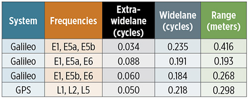
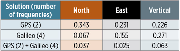
PPP Results. TABLE 1 shows the root mean square (RMS) of the errors and convergence times of the three components of position for the different configurations for the 550 points considered. Both single- and dual-constellation systems are able to provide a sub-decimeter-level accuracy after a few tens of minutes. On average, positioning with Galileo E1-E5a IF performs better that GPS L1-L5 IF: the Galileo solution is more accurate and converges faster than the GPS solution.

TABLE 1. Comparison between GPS-only, Galileo-only and GPS plus Galileo PPP results. RMS of the positioning errors and convergence times for the stations considered.

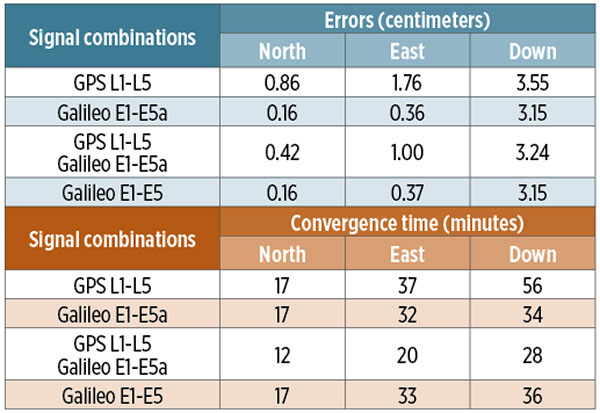
The reason for this behavior is the assumed lower noise on Galileo pseudoranges. It is well known that the quality of the pseudoranges affects the convergence time of the PPP solution.

For this reason, one would expect some improvements by employing the Galileo Alternative BOC (AltBOC) modulated E5 signal. Thanks to its very large signal bandwidth of at least 51 MHz, Galileo E5 is characterized by excellent rejection properties of both long-range and short-range multipath. However, as shown in Table 1, when comparing the PPP solutions obtained using the Galileo E1-E5 IF and E1-E5a IF combinations, they have nearly the same performance. The reason for this apparent contradiction can be found in the use of the IF combination with E1. Given that E1 represents the dominant source of error in the IF combinations, its noise is amplified by a factor of 2.34 in the IF combination with E5 and by a factor of 2.26 when combined with E5a. Also, the smaller errors (with respect to E1) in E5a are amplified by 1.26, while the one in E5 is amplified by 1.34. Therefore, depending on the noise level in the Galileo pseudoranges, there might be instances where the noise in the E1-E5 IF combination is close to the one in the E1-E5a IF combination.

The number and the geometry of the observed satellites also affect the convergence time. For this reason, when using the two systems together, the time the vertical errors take to go below 10 centimeters was reduced by 50 percent with respect to the GPS-only case and by 18 percent with respect to the Galileo-only case.

URBAN ENVIRONMENTS

The poor signal visibility and continuity associated with urban environments, together with the slow (re)convergence time of PPP, usually make the technique unsuitable for land navigation in cities. However, as demonstrated in the previous section, using a dual-constellation not only improves the visibility conditions, but also reduces the PPP convergence time. Therefore, it might be possible to extend the applicability of PPP to land navigation in certain urban areas.

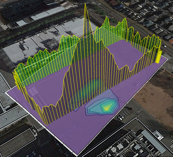
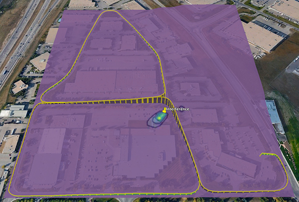
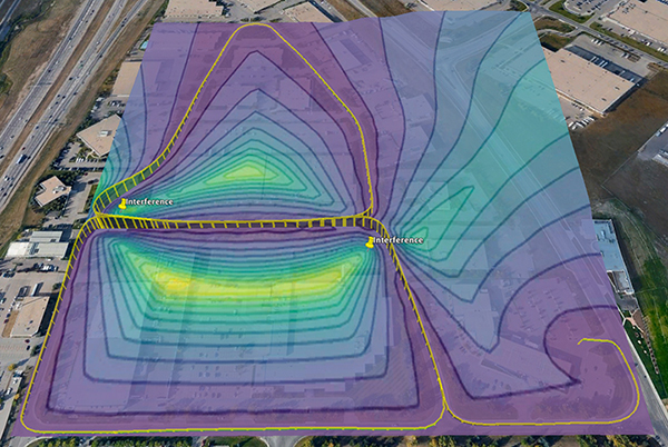
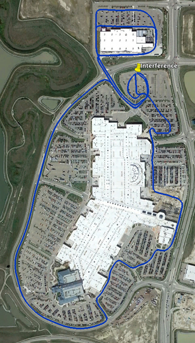
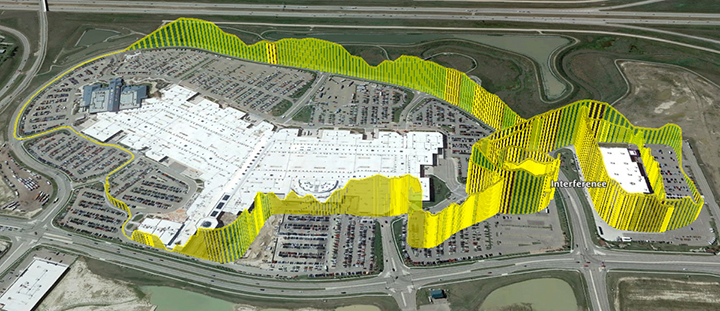
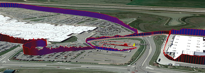
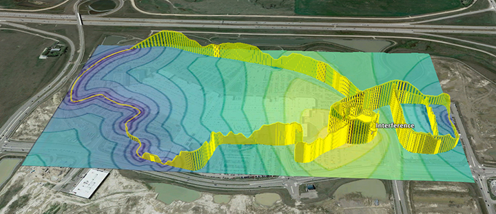
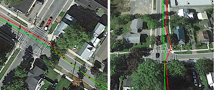
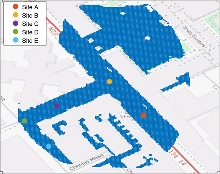
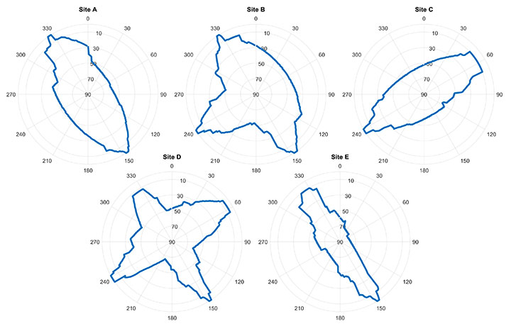
To assess the positioning performance of two-constellation GNSS in these constrained environments, we analyzed the signal availability and geometry of five different simulated sites in the neighborhood of the University College London (UCL) campus. We adopted building boundaries, which determine the minimum elevation angles above which GNSS signals can be received due to building obstruction. FIGURES 1 and 2 illustrate the location and the building boundaries for each site. FIGURE 3 shows the junction (site B) between Gower Street (site A) and University Street (site C).

FIGURE 1. Locations of the urban sites that are considered in the analysis.

FIGURE 2. Building obstruction masks controlling satellite visibility for each site.

FIGURE 3. Google Map image showing the junction (site B) between Gower Street (site A) and University Street (site C) in the midst of the University College London main campus.

When processing data from multi-constellation GNSS, the differences between the system time of the different constellations need to be considered. For this reason, when GPS and Galileo are used simultaneously for precise positioning, the Kalman filter state vector (in general) includes the three position components, the receiver clock offset, and the GPS-Galileo Time Offset (GGTO) — whether or not a predicted value might be available in a navigation message from one of the constellations. On the other hand, in PPP processing, the multi-constellation precise products used are based on the same system time, and therefore, in theory, it is not necessary to estimate the GGTO. However, existing intersystem biases may affect the PPP performance, and so it is advisable to estimate them in the Kalman filter.

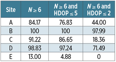
Traditionally in PPP, the state vector also includes the residual zenith wet tropospheric delay and the carrier-phase ambiguities. Therefore, the minimum number of satellites required for GPS plus Galileo PPP is six. The geometry conditions are also an important factor for assessing the GNSS positioning performance. For land navigation, the horizontal dilution of precision (HDOP), which provides information about the achievable horizontal precision (and, assuming a bias-free solution, accuracy), is particularly relevant. For many land applications, such as precision agriculture and urban positioning, horizontal accuracy is more critical than vertical accuracy. Assuming that the ranging error in the carrier phase is 20 centimeters, to have decimeter-level horizontal accuracy HDOP needs to be no larger than 5. In most cases, HDOP values as small as 2 are desired.

TABLE 2 gives an overview of the visibility and geometry conditions at the selected sites. A dual-constellation (GPS and Galileo) receiver placed at one of the two road junctions will always, or almost always, see at least six satellites with an HDOP better than 5. At sites A and C, these minimum requirements for signal availability and geometry are met for more than 75 percent of the day. Obstructions due to high buildings, such as at site E, allows us to have at least six satellites for only 13 percent of the time.

TABLE 2. Percentage of epochs in 24 hours for which dual-constellation GNSS meets the minimum visibility (number of satellites, N) and geometry requirements (horizontal dilution of precision, HDOP).

From our preliminary study, it seems clear that high-accuracy positioning in urban environments is possible, but only in some areas where buildings are relatively short, providing good signal availability and geometry. Things can slightly improve by considering additional systems, such as GLONASS and BeiDou, and by exploiting the non-line-of-sight (reflected) signals. However, it is well known that an additional obstacle for PPP in urban environments is signal discontinuity. Indeed, when a GNSS receiver loses lock on the carrier, the positioning filter needs to be reinitialized, meaning that further tens of minutes are required before reconvergence.

To test the reconvergence time of PPP in transient signal environments, a pedestrian carrying a multi-GNSS receiver was simulated to be walking along the path in FIGURE 4. The receiver was simulated to be located for the first half hour of the simulation in the front yard of UCL’s Wilkins Building (where the simulation begins and ends), before starting to move. This is to allow the initial convergence of the PPP filter.

FIGURE 4. The measured trajectory of the simulated pedestrian kinematic test.

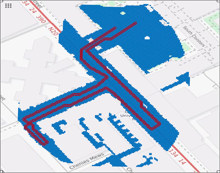
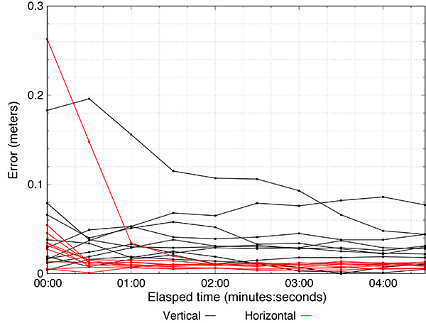
FIGURE 5 shows the visibility for a given GNSS satellite. Only the epochs when the receiver is moving are considered. Therefore, the first 30 minutes, when the receiver is static, are not included in the plot. Data gaps due to building obstructions are visible, with the largest being about 12 minutes and the average less than 2 minutes. As a consequence, the carrier-phase ambiguities need to be estimated all over again; and, as previously mentioned, this process usually requires tens of minutes before reconvergence.

FIGURE 5. Satellite availability during the kinematic test.

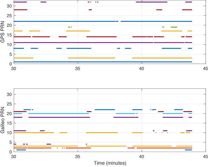
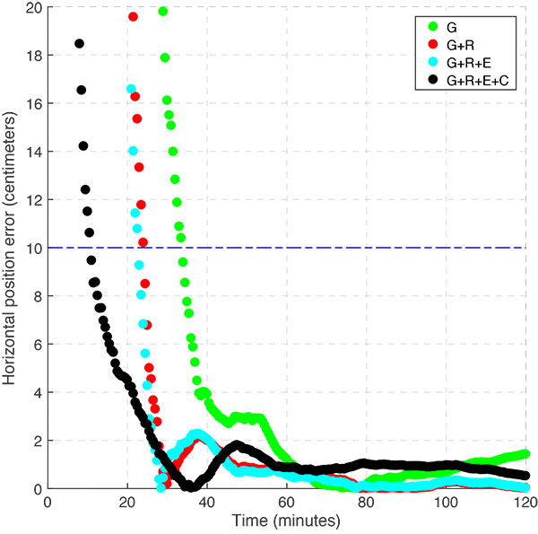
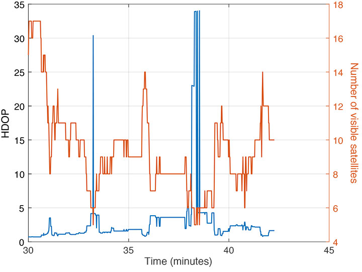
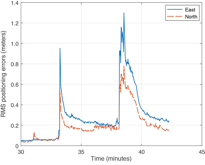
FIGURE 6 shows the HDOP and the number of visible satellites for the kinematic test, while FIGURE 7 shows the RMS, over 50 simulations, of the horizontal components of the positioning error when GPS L1 and L2 and Galileo E1 and E5, linearly combined into the IF combination, are processed in kinematic PPP mode with the POINT software. At the beginning of the kinematic test, when the HDOP is well below 5, the horizontal error is at the centimeter level, while, after 33 minutes from the beginning of the simulation, building obstructions don’t permit a converged solution below the 20-centimeter accuracy level.

FIGURE 6. Horizontal dilution of precision and number of visible satellites for the kinematic test.

FIGURE 7. RMS of the position errors for the kinematic test.

This short example clearly demonstrates that two-constellation PPP has, in theory, the potential to precisely navigate ground vehicles in some urban environments; however, it is too sensitive to signal discontinuity. Slow solution reconvergence to the few decimeter/centimeter level still represents the main limitation to the use of PPP for high-accuracy applications in cities. Nonetheless, GPS plus Galileo PPP easily enables sub-meter-level horizontal accuracy for most of the simulations we have carried out. After signal loss, it only took a few tens of seconds to have a horizontal accuracy of better than a meter.

SMOOTHED CORRECTIONS

As an alternative to ambiguity-fixing methods aimed to improve the (re)convergence time, we propose a method that mitigates the effect of the ionosphere and which thereby reduces the reconvergence time of the PPP solution after initial convergence has been achieved. In this new approach, while the two-frequency carrier phases are linearly combined in the traditional IF combination, the uncombined pseudoranges are corrected by a pre-smoothed ionospheric delay (via a Hatch filter), computed using the geometry-free combination of two-frequency pseudoranges.

Once the Hatch filter has converged, ideally we have IF pseudoranges with lower noise than the traditional ones. Therefore, in case the PPP filter needs to restart, we can obtain a quicker reconvergence thanks to the lower noise on the ionosphere-corrected pseudoranges. Indeed, provided that the signal gap is not very large, the ionosphere smoothing filter doesn’t need to be restarted from the raw values.

It is possible to predict the ionospheric delay computed from two-frequency carrier-phase measurements using a linear fitting model from previous measurements within a sliding time window. As an example, high-rate data recorded on July 25, 2017, from station DAEJ in Daejeon, Republic of Korea, were used to analyze the ionosphere prediction error.

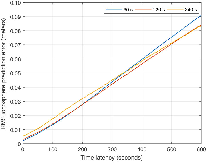
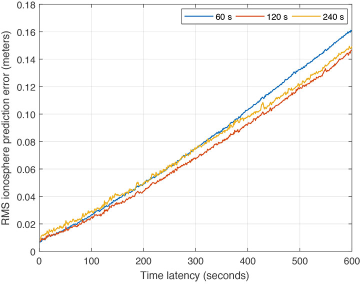
In FIGURES 8 and 9, the RMS of the prediction errors for different time windows have been plotted against the data gap length. The prediction error depends on both the time latency of the observation and the elevation angle of the satellite. It increases with the data gap length, but larger time windows can damp the divergence of the error. A time window of 120 seconds was used both for satellites above and below 30° elevation angle. In this case, the error for a 5-minute prediction is about 4 centimeters for a satellite above 30° and 7 centimeters for satellites with a low elevation angle. These values are much smaller than the noise in the pseudorange measurements and can, therefore, be neglected.

FIGURE 8. RMS of the prediction errors vs. data gap length for satellite elevation angles greater than 30°.

FIGURE 9. RMS of the prediction errors vs. data gap length for satellite elevation angles less than than 30°.

Multi-Frequency Combinations. The method introduced in the previous section allows users to be free from the constraint of IF observables and, therefore, to look for multi-frequency combinations aimed to minimize the noise on the pseudoranges. The next-generation GNSS satellites will broadcast open signals over three frequencies. The triple-frequency, geometry-preserving combination aimed to reduce the noise, instead of mitigating the ionosphere, can be used for positioning purposes.

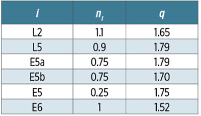
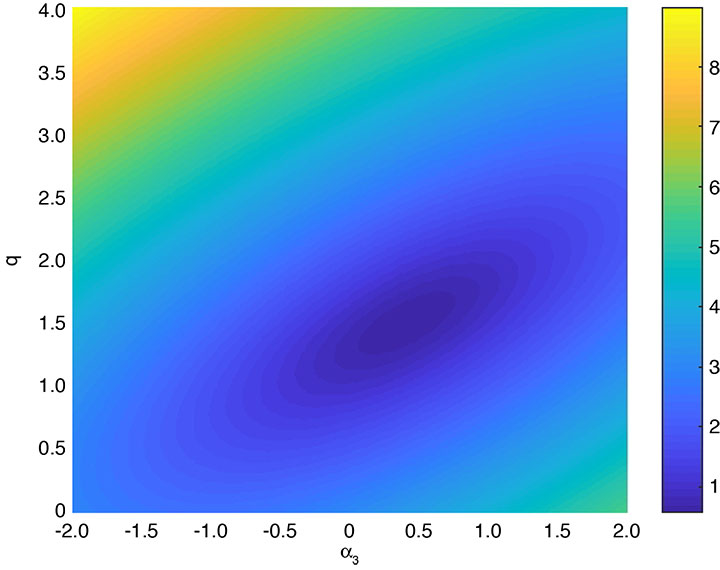
TABLE 3 summarizes the assumed values for the ratios n_i between the noise on different GPS and Galileo pseudoranges and the ones on L1/ E1. FIGURE 10 shows a color map of the noise amplification factor associated with different linear combinations between GPS L1, L2 and L5. The x-axis is α₃, the coefficient multiplying the pseudorange on L5 in the combination, while the y-axis is the ionosphere amplification factor of the triple-frequency combination with respect to L1, q. The noise for this combination can be as little as 0.57 times the noise on L1, while the corresponding ionosphere amplification factor is 1.49. Once the smoothed ionosphere correction has converged, we can potentially have an IF pseudorange 81 percent less noisy than the L1-L2 IF, and, therefore, a much faster reconvergence.

TABLE 3. Assumed noise, n_i, on GPS and Galileo pseudoranges, i, and their ionospheric delay, q, with respect to L1/ E1.

FIGURE 10. Geometry-preserving surface in the space q-α₃-n (ionosphere amplification factor – L5 pseudorange multiplier – noise amplification factor) for GPS L1-L2-L5 combinations.

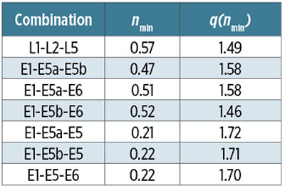
Similar conclusions can be drawn by considering Galileo signals. Using triple-frequency combinations with E1, E5a and E5b, we can obtain 81 percent less noise than E1-E5a IF, while a reduction of the noise in the IF pseudorange up to 90 percent was observed using E5 alone. Triple-frequency combinations involving E5 don’t bring such large improvements with respect to using E5 alone. Indeed, a maximum of 16 percent less noise can be registered when combining E1, E5a and E5 with respect to the E5 uncombined case. TABLE 4 illustrates the minimum noise amplification factor for each triple-frequency combination and its ionosphere amplification factor.

TABLE 4. Minimum noise achievable through GPS and Galileo triple-frequency pseudorange combinations and their ionospheric delay with respect to L1/ E1.

The noise associated with the ionosphere-corrected multi-frequency pseudorange combination is as large as meter level before converging to centimeter level. For this reason, a proper weighting method, which considers the varying noise on the ionosphere correction, needs to be employed.

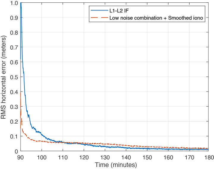
To test the benefit of the new approach for the reconvergence time, three hours of simulated GPS and Galileo data from a static site in La Misere, Seychelles, were processed with the POINT software in kinematic mode. After 90 minutes, the PPP filter was forced to restart to simulate reconvergence. The multipath time constant was set to 5 seconds, which is a typical value for kinematic multipath. The performance of the traditional L1- L2 IF combination was compared with the triple-frequency pseudorange combination, corrected by the smoothed ionosphere delay coming from the Hatch filter.

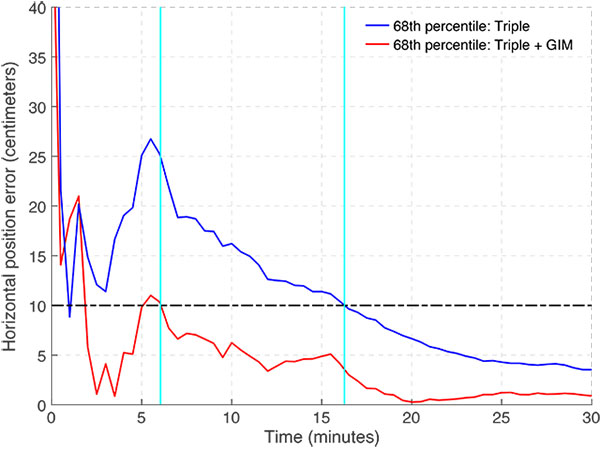
FIGURE 11 shows the precision (RMS error over 50 simulations) of the horizontal components after filter restart. The new approach has much faster reconvergence than the traditional PPP method based on the IF combination. Indeed, while the traditional method takes about 11 minutes to have a horizontal error below 10 centimeters, using the low-noise combination, this accuracy is achieved after 171 seconds. Even better performance can be achieved considering the Galileo E5 signal (see FIGURE 12).

FIGURE 11. RMS error of the horizontal position components of static site using GPS data after filter restart.

FIGURE 12. RMS error of the horizontal position components of static site using Galileo data after filter restart.

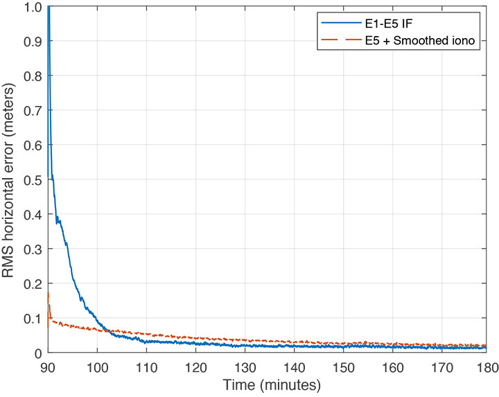
The E1-E5 IF combination requires 10 minutes for the horizontal convergence, while using E5 with the Hatch filter we have the horizontal solution converged in about 30 seconds. It is worth noticing that in the presence of static multipath, the proposed weighting method may lead to an overly optimistic weighting of the pseudorange measurements in the PPP filter and to a slower reconvergence of the positioning solution. Indeed, the long correlation time in the static multipath, of the order of a few minutes, makes it hard to filter out by the Hatch filter, hence the corrected measurements have larger errors than expected.

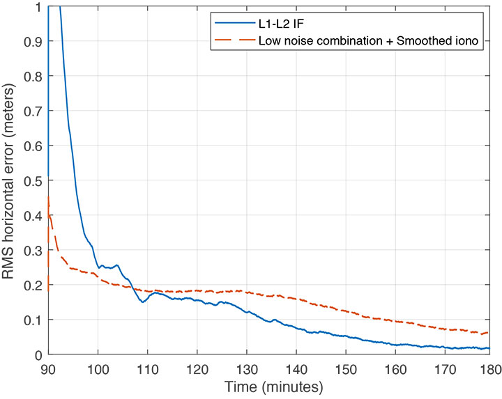
The effect of static multipath in the new configuration is visible in FIGURE 13, where the reconvergence of the horizontal component for the L1-L2 IF combination is compared with the new approach. In this case, the time constant of the simulated multipath was set to 1 minute. In this scenario, the triple-frequency low-noise combination corrected by the smoothed ionosphere combination quickly converges below 20 centimeters; however, it takes significantly longer than the L1-L2 IF combination to reach the 10-centimeter accuracy level.

FIGURE 13. RMS error of horizontal position component of static site using GPS data after filter restart with 1-minute multipath time constant.

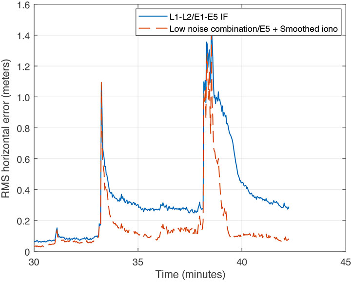
Also, the new method was tested with the kinematic simulation as in the previous section. Here, the GPS triple-frequency combined pseudorange and Galileo E5 pseudorange (both corrected with the smoothed ionosphere) are processed in kinematic PPP mode with the POINT software. FIGURE 14 compares the RMS of the horizontal errors with the IF configuration. Less than a minute after the receiver lost lock on the satellites, the solution reconverged below the 20-centimeter level, while it took less than 30 seconds to go below 50 centimeters.

FIGURE 14. RMS error of the horizontal position components of kinematic trajectory using GPS and Galileo data and the smoothed ionosphere approach after filter restart.

CONCLUSIONS

In this article, we described a comparison that we carried out between GPS-only, Galileo-only and GPS plus Galileo PPP. Results based on simulated open-sky conditions demonstrated that Galileo performs better than GPS thanks to an assumed lower E1-E5a IF noise with respect to L1-L5. Two-constellation PPP enables faster (re)convergence compared to the single constellation case.

An analysis of GNSS signal availability, continuity and satellite geometry was also performed to study the feasibility of PPP in urban environments. Preliminary results, based on simulations, showed that dual-constellation (GPS plus Galileo) PPP is possible in urban areas with relatively short buildings in which a satellite minimum availability requirement is met most of the time. However, signal discontinuity still represents the major problem for traditional PPP in urban environments, due to long reconvergence times.

Finally, we proposed a new PPP configuration based on triple-frequency combinations, intended to minimize the noise on the pseudorange and corrected by a smoothed ionospheric delay. This configuration seems to provide faster reconvergence than the traditional PPP with the IF combination if applied to kinematic scenarios. In static applications, the very slow varying multipath error makes the proposed weighting method, based on the error in the smoothed ionosphere correction, overly optimistic. In such cases, the IF combination reconverges more quickly to high-accuracy levels better than 20 centimeters.

ACKNOWLEDGMENTS

The research described in this article was sponsored through a studentship agreement between the University of Nottingham and Rockwell Collins UK Limited. The article is based on the paper “Multi-Frequency Precise Point Positioning Using GPS and Galileo Data with Smoothed Ionospheric Corrections” presented at the 2018 IEEE/ION Position, Location and Navigation Symposium, held in Monterey, California, April 23–26, 2018. All figures attributed to the authors unless otherwise specified.

MANUFACTURERS

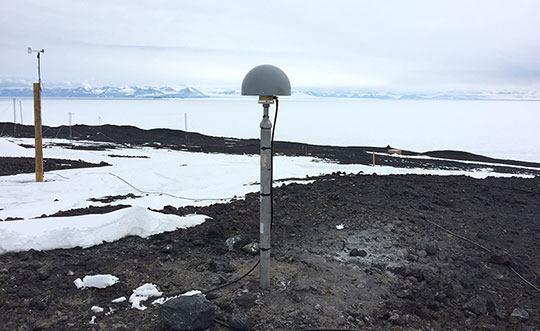
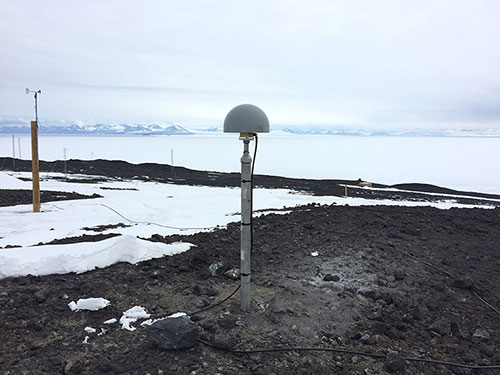
The receiver at station DAEJ is a Trimble NetR9.

FRANCESCO BASILE is a postgraduate research student at the Nottingham Geospatial Institute of the University of Nottingham in the United Kingdom. He received his M.Sc. in space and astronautic engineering from the University of Rome – La Sapienza and his B.Sc. in aerospace engineering from the University of Naples – Federico II, both in Italy.

TERRY MOORE is the director of the Nottingham Geospatial Institute where he is the Professor of Satellite Navigation. He is a fellow and the president of the Royal Institute of Navigation (RIN) and also a fellow and a member of council of the Institute of Navigation (ION).

CHRIS HILL is an associate professor in the Faculty of Engineering at the University of Nottingham and a member of the Nottingham Geospatial Institute research group. He holds a Ph.D. in satellite laser ranging and he is a fellow of the RIN.

GARY MCGRAW is a technical fellow with the Rockwell Collins Advanced Technology Center in Cedar Rapids, Iowa. McGraw is a fellow of the ION and is a senior member of the IEEE.

ANDREW JOHNSON is a chief engineer at Rockwell Collions UK in Winnersh, Berkshire, United Kingdom. Johnson has a B.Sc. in electronic and electrical engineering from the University of Surrey in Guildford, United Kingdom.

FURTHER READING
- Authors’ Conference Paper
“Multi-Frequency Precise Point Positioning Using GPS and Galileo Data with Smoothed Ionospheric Corrections” by F. Basile, T. Moore, C. Hill, G. McGraw and A. Johnson in Proceedings of PLANS 2018, the Institute of Electrical and Electronics Engineers / Institute of Navigation Position, Location and Navigation Symposium, Monterey, California, April 23–26, 2018, pp. 1388–1398, doi: 10.1109/PLANS.2018.8373531.
- Multi-Constellation Use in Built-up Areas
“Making It Better: Low-Cost Single-Frequency Positioning in Urban Environments” by I. Smolyakov and R.B. Langley in GPS World, Vol. 29, No. 5, May 2018, pp. 42–48.

“Quo Vademus: Future Automotive GNSS Positioning in Urban Scenarios” by M. Escher, M. Stanisak and U. Bestmann in GPS World, Vol. 27, No. 5, May 2016, pp. 46–52.

“Multi-Constellation GNSS Performance Evaluation for Urban Canyons Using Large Virtual Reality City Models” by L. Wang, P.D. Groves and M.K. Ziebart in Journal of Navigation, Vol. 65, No. 3, July 2012, pp. 459–476, doi: 10.1017/S0373463312000082.

“Potential Benefits of GPS/GLONASS/GALILEO Integration in an Urban Canyon – Hong Kong” by S. Ji, W. Chen, X. Ding, Y. Chen, C. Zhao and C. Hu in Journal of Navigation, Vol. 63, No. 4, October 2010, pp. 681–693, doi: 10.1017/S0373463310000081.
- Multi-Constellation Use in Aviation Applications
“Assessment of Alternative Positioning Solution Architectures for Dual Frequency Multi-Constellation GNSS/SBAS” by G. McGraw, B.A. Schnaufer, P.Y. Hwang and M.J. Armatys in Proceedings of ION GNSS+ 2013, the 26th International Technical Meeting of the Satellite Division of The Institute of Navigation, Nashville, Tennessee, Sept. 16–20, 2013, pp. 223–232.
- Advances in Precise Point Positioning
“More Is Better: Instantaneous Centimeter-Level Multi-Frequency Precise Point Positioning” by D. Laurichesse and S. Banville in GPS World, Vol. 29, No. 7, July 2018, pp. 42–47.

“Where Are We Now, and Where Are We Going?: Examining Precise Point Positioning Now and in the Future” by S. Bisnath, J. Aggrey, G. Seepersad and M. Gill in GPS World, Vol. 29, No. 3, March 2018, pp. 41–48.

“Undifferenced GPS Ambiguity Resolution Using the Decoupled Clock Model and Ambiguity Datum Fixing” by P. Collins, S. Bisnath, F. Lahaye, and P. Héroux in Navigation, Vol. 57, No. 2, Summer 2010, pp. 123–135, doi: 10.1002/j.2161-4296.2010.tb01772.x.

“Integer Ambiguity Resolution on Undifferenced GPS Phase Measurements and Its Application to PPP and Satellite Precise Orbit Determination” by D. Laurichesse, F. Mercier, J.-P. Berthias, P. Broca and L. Cerri in Navigation, Vol. 56, No. 2, Summer 2009, pp. 135–149, doi: 10.1002/j.2161-4296.2009.tb01750.x.
- Hatch Filter
“Combinations of Observations” by A. Hauschild, Chapter 20 in Springer Handbook of Global Navigation Satellite Systems, edited by P.J.G. Teunissen and O. Montenbruck, published by Springer International Publishing AG, Cham, Switzerland, 2017.

“The Synergism of GPS Code and Carrier Measurements” by R. Hatch in Proceedings of the Third International Geodetic Symposium on Satellite Doppler Positioning, Las Cruces, New Mexico, Feb. 8–12, 1982, Vol. II, pp. 1213–1232.
- Dilution of Precision
“Dilution of Precision” by R.B. Langley in GPS World, Vol. 10, No. 5, May 1999, pp. 52–59.
- Kalman Filtering
“Least-Squares Estimation and Kalman Filtering” by S. Verhagen and P.J.G. Teunissen, Chapter 22 in Springer Handbook of Global Navigation Satellite Systems, edited by P.J.G. Teunissen and O. Montenbruck, published by Springer International Publishing AG, Cham, Switzerland, 2017.

“The Kalman Filter: Navigation’s Integration Workhorse” by L.J. Levy in GPS World, Vol., No., September 1997, pp. 65–71.
October 9, 2018
Innovation: The International GNSS Service
25 years on the path to multi-GNSS

As Galileo, BeiDou, the Quasi-Zenith Satellite System, the Indian Regional Navigation Satellite System, and a variety of satellite-based augmentation systems join GPS and GLONASS, we help celebrate the coming 25th anniversary of the IGS as a truly multi-GNSS service.

Editor’s note: Tables 1 and 3 in the print version of this article contain some incorrect values and missing designators. These errors have been corrected in the tables below.

INNOVATION INSIGHTS by Richard Langley

A QUARTER OF A CENTURY. That is how old the International GNSS Service (IGS) will be on Jan. 1, 2019. Conceived in the early 1990s as the International GPS Service for Geodynamics, the IGS continues to be the global standard bearer in providing receiver data, satellite orbit and clock products and other resources with the highest possible precision and accuracy. I remember the discussions that took place at international conferences about the need for such a service to provide the necessary data to advance our understanding of plate tectonics and other Earth-related phenomena. And this was well before GPS was officially declared fully operational in 1995. Remember, surveyors and geodesists were early adopters of GPS, making use of the technology even when only a partial GPS constellation was in place.

The initial ideas for the IGS were laid out in an article published in GPS World in February 1993 entitled “Geodynamics: Tracking Satellites to Monitor Global Change.” But the services provided by the IGS extended well beyond the needs of the geodynamics research community, and so its name was shortened to just the International GPS Service. When GLONASS data and products became available, the name was further changed to its current moniker.

One of the IGS’s notable achievements has been in advancing GNSS standards such as the Receiver-Independent Exchange format for receiver data and other information. The need for such a standard was clear even before the formation of the IGS, and it was documented in this column in the July 1994 issue of GPS World (“RINEX: The Receiver-Independent Exchange Format”). We continued to cover the evolution of the IGS over the years with, for example, the article “The International GNSS Service: Any Questions?” in the January 2007 issue of the magazine.

And now, as Galileo, BeiDou, the Quasi-Zenith Satellite System, the Indian Regional Navigation Satellite System, and a variety of satellite-based augmentation systems join GPS and GLONASS, we help celebrate the coming 25th anniversary of the IGS as a truly multi-GNSS service.

For going on 25 years, the International GNSS Service (IGS) has carried out its mission to advocate for, and provide, freely and openly available high-precision GNSS data, as well as derived operational data products, including satellite ephemerides, Earth rotation parameters, station coordinates and clock information. The IGS is a self-governed, voluntary federation of more than 300 contributing organizations from more than 100 countries around the world that collectively operate a global infrastructure of tracking stations, data centers and analysis centers to provide high-quality GNSS data products. The IGS products are provided openly for the benefit of all scientific, educational and commercial users.

The IGS was first approved by its parent organization, the International Association of Geodesy (IAG), at a scientific meeting in Beijing, China, in August 1993. A quarter of a century later, the IGS community gathers for a workshop in Wuhan, China, this November to blaze a path to multi-GNSS through global collaboration.

As a key component of the IAG’s global geodetic infrastructure, the IGS contributes to, extends and densifies the International Terrestrial Reference Frame (ITRF) of the International Earth Rotation and Reference Systems Service (IERS). The ITRF provides an accurate and consistent spatial frame for referencing positions at different times and in different locations around the world.

In addition, IGS products enable the use of GNSS technologies for scientific applications such as the monitoring of solid Earth deformations, monitoring of Earth rotation and variations in the liquid Earth, and for scientific satellite orbit determinations, precise timing, ionosphere monitoring and water vapor measurements.

IGS products are also considered critical by surveying, geomatics and geo-information users around the world, who rely on them on a daily basis to improve efficiency. Many applications that require reliable, accurate GNSS positioning in construction, agriculture, mining, exploration and transportation also benefit from the IGS.

Community Collaboration

At the heart of the IGS is a strong culture of sharing expertise, infrastructure and other resources for the purpose of encouraging global best practices for developing and delivering GNSS data and products all over the world. The collaborative nature of the IGS community leverages this diversity to integrate and make full use of all available GNSS technologies while promoting further innovation.

More than 15,000 geodetic community members, some of whom comprise the backbone of the worldwide geodetic community, ensure that new technologies and systems are integrated into operational IGS products. Responsive to this innovation, the IGS develops and publicly releases standards, guidelines and conventions for the collection and use of GNSS data and the aforementioned products.

The IGS strives to maintain an international federation with committed contributions from its members. Participation of individuals and organizations is often driven by user needs, a key characteristic of the inclusive culture within the IGS.

Structure of the IGS

The IGS consists of a central bureau, a global network of GNSS stations, data and analysis centers and a number of working groups all coordinated and overseen by a governing board.

Central Bureau. The IGS Central Bureau (CB) functions as the secretariat of the IGS, providing continuous management and technology to sustain the multifaceted efforts of the IGS in perpetuity. The CB responds to the directives and decisions of the IGS governing board. It coordinates the IGS tracking network and operates the CB information system, the principal information portal where the IGS web, FTP and mail services are hosted (www.igs.org). The CB also represents the outward face of IGS to a diverse global user community, as well as the general public. The CB office is hosted at the California Institute of Technology/Jet Propulsion Laboratory in Pasadena, California. It is funded principally by the U.S. National Aeronautics and Space Administration (NASA), which generously contributes significant resources to advance the IGS.

The IGS Network. The foundation of the IGS is a global network of more than 500 permanent and continuously operating stations of geodetic quality. These stations track signals from GPS, and increasingly also track signals from GLONASS, Galileo, BeiDou, the Quasi-Zenith Satellite System (QZSS), the Indian Regional Navigation Satellite System (IRNSS; also known as NavIC: Navigation with Indian Constellation), as well as space-based augmentation systems (SBAS).

FIGURE 1 shows the recent state of the IGS network, indicating which stations are GPS only, GPS+GLONASS and multi-GNSS. FIGURE 2 is a photo of the IGS station ARHT at McMurdo Station, Antarctica.

FIGURE 1 . The extent of the IGS network in 2017, showing the locations of stations monitoring just GPS, GPS and GLONASS, and GPS and GLONASS plus at least one other constellation. (Map: IGS)

FIGURE 2. The consistency of the final GPS satellite orbit solutions from individual IGS analysis centers over the past 25 years. Each line depicts the solution of one analysis center, as compared to the weighted mean. COD: Center for Orbit Determination in Europe, EMR: Natural Resources Canada (formerly Energy, Mines and Resources Canada), ESA: European Space Agency, GFZ: GeoForschungsZentrum (German Research Centre for Geosciences); GRG: Centre National d’Etudes Spatiales (Groupe de Recherche de Géodésie Spatiale); JPL: Jet Propulsion Laboratory; MIT: Massachusetts Institute of Technology; NGS: National Geodetic Survey; SIO: Scripps Institution of Oceanography; IGR: IGS rapid product. (Graph courtesy of T. Herring, MIT and M. Moore, Geoscience Australia)

The IGS is a critical component of the IAG’s Global Geodetic Observing System (GGOS), where it encourages and advocates for geometrical linkages of GNSS with other precise geodetic observing techniques, including satellite and lunar laser ranging, very long baseline interferometry and Doppler Orbitography and Radio Positioning Integrated by Satellite (DORIS). These linkages are fundamental to generating and accessing the ITRF.

Data and Analysis Centers. Lots of hard work and dedication from IGS contributing organizations goes into the fabrication of IGS products, which start at the tracking network, then are collected by data centers and sent to analysis centers. At these centers, the data are compared and combined by the analysis center coordinator, and finally made available as IGS products.

The IGS ensures high reliability by building redundancy into all of its components. In 1994, the IGS started with a network of about 40 stations; today, more than 500 receivers are included in the network. Critical to this activity are three categories of data center — operational, regional and global. At the ground level are operational data centers, which are in direct contact with IGS tracking sites and are responsible for such efforts as station monitoring and local archiving of GNSS tracking data. Operational data centers also validate, format, exchange and compress data. Regional data centers then collect tracking data from multiple operational data centers or stations, maintaining a local archive and providing online access to their data.

The six global data centers receive, retrieve, archive and provide online access to tracking data from operational and regional data centers. These global data centers are also responsible for archiving and backing up IGS data and products, and maintaining a balance of data holdings across the IGS network.

Analysis centers then receive and process tracking data from one or more data centers to generate IGS position, orbit and clock products. These products are produced in ultra-rapid, rapid, final and reprocessed versions for each analysis center.

FIGURE 3 shows the huge improvement in the precision and accuracy of the final orbit submissions from the analysis centers over the past 25 years.

Associate analysis centers produce specialized products, such as ionospheric information, tropospheric parameters or station coordinates and velocities for global and regional sub-networks. Regional and global network associate analysis centers complement this work as new capabilities and products emerge within the IGS.

FIGURE 3. The antenna of IGS station ARHT at McMurdo Station, Antarctica. (Photo: IGS)

Products from each analysis center are then combined into a single set of orbit and clock products by the analysis center coordinator, who monitors and assists the activities of analysis centers to ensure IGS standards for quality control, performance evaluation and analysis are successfully executed. The different analysis solutions ultimately verify the accuracy of IGS products, provide important redundancy in the case of errors in a particular solution, and average out modeling deficiencies of a particular software package.

TABLE 1 shows the quality of service characteristics of the various IGS GPS and GLONASS orbit and clock products. Similarly, TABLES 2, 3 and 4 show the characteristics of the tracking station coordinates, Earth rotation parameters and atmospheric parameters. See www.igs.org/products for further details.

TABLE 1. Quality of service characteristics for IGS orbit and clock products relating to GPS and GLONASS satellite orbits and satellite (sat.) and station (stn.) clocks as of 2017. (Data: IGS)

TABLE 2. Quality of service characteristics for tracking station positions and velocities. (Data: IGS)

TABLE 3. Quality of service characteristics for Earth rotation parameters: polar motion coordinates and rates of change and length-of-day (µas = microarcsecond). (Data: IGS)

TABLE 4. Quality of service characteristics for atmospheric parameters: tropospheric zenith path delay and gradients and global grids of total electron content. (Data: IGS)

Working Groups and Projects

The IGS technical working groups (WGs) focus on topics of particular interest to the IGS, and consider various aspects of product generation and monitoring. The current working groups of the IGS span topics from antennas to tide gauges.

Antenna Working Group. To increase the accuracy and consistency of IGS products the Antenna WG coordinates research on GNSS receiver and satellite antenna phase-center determination. The group manages official IGS receiver and satellite antenna files and their formats.

Bias and Calibration Working Group. Different GNSS observables are subject to different satellite biases, which can degrade the IGS products. The Bias and Calibration WG coordinates research in the field of GNSS bias retrieval and monitoring.

Clock Products Working Group. This group is responsible for aligning the combined IGS products to a highly precise timescale traceable to the world standard: Coordinated Universal Time (UTC). The IGS clock product coordinator forms the IGS timescales based on the clock solutions of IGS analysis centers, and IGS rapid and final products are aligned to these timescales.

Data Center Working Group. The Data Center WG works to improve the provision of data and products from the operational, regional and global data centers, and recommends new data centers to the IGS governing board.

Joint GNSS Monitoring and Assessment Working Group. This working group, in conjunction with a joint trial project with International Committee on GNSS’s (ICG) International GNSS Monitoring and Assessment (IGMA) Task Force, seeks to install, operate and further develop a GNSS Monitoring and Assessment Trial Project.

GNSS Performance Monitoring ICG-IGS Joint Trial Project. The quality of navigation signals enables numerous applications, including worldwide time and frequency transfer and GPS meteorology. This project of the IGMA task force, coordinated in partnership with the IGS, focuses on monitoring GNSS constellation status.

Ionosphere Working Group. This group produces global ionosphere maps of ionosphere vertical total electron content (TEC). A major task of the Ionosphere WG is to make available global ionosphere maps from the TEC maps produced independently by ionosphere associate analysis centers within the IGS.

FIGURE 4 shows an example TEC map recomputed from data collected on March 17, 2015. The large values of TEC in the ionosphere’s equatorial anomaly are plainly visible.

FIGURE 4. An example total electron content map recomputed from data collected on March 17, 2015. TECU: total electron content units. (Image: IGS)

Multi-GNSS Working Group. This group supports the Multi-GNSS Experiment (MGEX) Project by facilitating estimation of intersystem biases and comparing the performance of multi-GNSS equipment and processing software. The MGEX Project was established to track, collate and analyze all available GNSS signals including those from BeiDou, Galileo and QZSS in addition to GPS and GLONASS.

Reference Frame Working Group. This working group combines solutions from the IGS analysis centers to form the IGS station positions and velocity products, and Earth rotation parameters for inclusion in the IGS realization of ITRF. A new reference frame, called IGS14, was adopted on Jan. 29, 2017 (GPS Week 1934). At the same time, an updated set of satellite and ground antenna calibrations, igs14.atx, was implemented.

Real-Time Working Group. The Real-Time WG supports the development and integration of real-time technologies, standards and infrastructure to produce high-accuracy IGS products in real time. The group operates the IGS Real-Time Service (RTS) to support precise point positioning (PPP) at global scales, in real time.

RINEX Working Group. The RINEX-WG jointly manages the Receiver-Independent Exchange (RINEX) format with the Radio Technical Commission for Maritime Services Special Committee 104 (RTCM-SC104). RINEX has been widely adopted as an industry standard for archiving and exchanging GNSS observations, and newer versions support multiple GNSS constellations. Recently, the IGS governing board agreed to adopt the official RINEX V3.04 format, handling the ability for nine-character station ID and fixing the definition of GNSS reference time scales.

Space Vehicle Orbit Dynamics Working Group. This group brings together IGS groups working on orbit dynamics and attitude modeling of spacecraft. This work includes the development of force and attitude models for new GNSS constellations to fully exploit all new signals with the highest possible accuracy.

Troposphere Working Group. The Troposphere WG supports development of IGS troposphere products by combining troposphere solutions from individual analysis centers to improve the accuracy of PPP solutions. The goal of the Troposphere WG is to improve the accuracy and usability of GNSS-derived troposphere estimates.

Tide Gauge (TIGA) Working Group. When studying sea level changes, where the GPS height of the benchmark is used for defining an absolute sea-level datum, problems occur when correcting the time series for height changes of the benchmark. TIGA is a pilot study for establishing a service to analyze GPS data from stations at or near tide gauges in the IGS network to support accurate measurement of sea-level change across the globe.

A Multi-GNSS IGS Network

The development of a multi-GNSS sub-network within the greater IGS network, led by the MGEX Project, develops the IGS’s capability to operate with multiple GNSS constellations. It has 223 multi-GNSS-capable (GPS + GLONASS + at least one other constellation) stations. Also, the number of IGS stations capable of real-time data streaming in support of the IGS Real-Time Project has increased to 195.

MGEX was founded in 2012 to build a network of GNSS tracking stations, characterize the space segment and user equipment, develop theory and data-processing tools, and generate data products for emerging satellite systems. The stations within its network contain a diverse assortment of receiver and antenna equipment, which are recognized and characterized by the IGS in equipment description files. Other than GPS and GLONASS, no combination process has yet been implemented within IGS for precise orbit and clock products of the other, newer, constellations. Despite this, cross-comparison among analysis centers, as well as with satellite laser ranging, has been used to assess the precision or accuracy for various products.

The growing role of multi-GNSS within the IGS network was benchmarked by the transition of MGEX to official IGS project status in 2016. For the sake of consistency, and as a nod to its heritage, use of the acronym “MGEX” has been retained.

Making Strides in Real Time

Through the Real-Time Service (RTS), the IGS extends its capability to support applications requiring real-time access to IGS products. The RTS is a GNSS orbit and clock correction service that enables PPP and related applications, such as time synchronization and disaster monitoring, at worldwide scales. The RTS is based on the IGS global infrastructure of network stations, data centers and analysis centers that provide world-standard high-precision GNSS data products.

The RTS is currently offered as a GPS-only operational service, but GLONASS is initially being offered as an experimental product for the development and testing of applications. GLONASS will be included within the service when the IGS is confident that a sufficient number of analysis centers can ensure solution reliability and availability. Other GNSS constellations will be added as they become available.

Engagement with the United Nations

The IGS engages with diverse organizations, outside of the immediate precise GNSS community, that have an interest in geodetic applications of GNSS. Notably, the IGS has supported the development of the Global Geodetic Reference Frame resolution, roadmap and implementation plan within the United Nations Global Geospatial Information Management (GGIM) Committee of Experts.

The IGS also works with the United Nations Office for Outer Space Affairs (UNOOSA) International Committee on GNSS (ICG) to develop common understandings of the requirements for multiple system monitoring through the joint pilot project with the ICG’s IGMA subgroup. The IGS also co-chairs ICG Working Group D, which focuses on reference frames, timing and applications.

A Multi-GNSS Future

Though the accuracy of current IGS multi-GNSS products lags behind standard IGS products for GPS and GLONASS, multi-GNSS paves the way for complete exploitation of new signals and constellations in navigation, surveying, geodesy and remote sensing.

IGS also looks externally to other techniques through its participation in the IAG’s GGOS, which has illuminated how satellite laser ranging observations to GNSS satellites improves our understanding of observational errors and thus drives further improvement of IGS position, clock and orbit products.

As it enters its second quarter-century, the IGS is evolving into a truly multi-GNSS service. For 25 years, IGS data and products have been made openly available to all users for use without restriction, and continue to be offered free of cost or obligation. In turn, users are encouraged to participate within the IGS, or otherwise contribute to its advancement.

Acknowledgements

The authors gratefully acknowledge the contributions of the IGS governing board and associate members in the drafting of this article. Special thanks to Anna Riddell and Grant Hausler, who, along with Gary Johnston, have an extensive chapter on IGS in the Springer Handbook of Global Navigation Satellite Systems, published in 2017 by Springer (see Further Reading). This book chapter is the new recommended official citation for publications referencing IGS data, products and other resources.

Allison Craddock a member of the Geodynamics and Space Geodesy Group in the Tracking Systems and Applications Section at the NASA Jet Propulsion Laboratory in Pasadena, California. She is the director of the IGS Central Bureau, manager of external relations for the International Association of Geodesy’s Global Geodetic Observing System, and staff member of the NASA Space Geodesy Program.

Gary Johnston is the head of the National Positioning Infrastructure Branch at Geoscience Australia. Johnston is the chair of the IGS governing board and the co-chair of the Subcommittee on Geodesy under the United Nations Global Geospatial Information Management committee of experts.

FURTHER READING
- GNSS Handbook Chapter on IGS
“The International GNSS Service” by G. Johnston, A. Riddell and G. Hausler, Chapter 33 in Springer Handbook of Global Navigation Satellite Systems, edited by P.J.G. Teunissen and O. Montenbruck, published by Springer International Publishing AG, Cham, Switzerland, 2017.
- IGS: Past, Present and Future
International GNSS Service Strategic Plan 2017, edited by the IGS Central Bureau.

International GNSS Service Technical Report 2017 (IGS Annual Report), edited by A. Villiger and R. Dach, published by IGS Central Bureau and University of Bern, Bern Open Publishing, Bern, Switzerland, 2018, doi: 10.7892/boris.116377. Includes reports from analysis centers, data centers and working groups.

“The International GNSS Service: Any Questions?” by A.W. Moore in GPS World, Vol. 18, No. 1, January 2007, pp. 58–64.

“Geodynamics: Tracking Satellites to Monitor Global Change” by G. Beutler, P. Morgan and R.E. Neilan in GPS World, Vol. 4, No. 2, February 1993, pp. 40–46.
- IGS Multi-GNSS Experiment
IGS White Paper on Satellite and Operations Information for Generation of Precise GNSS Orbit and Clock Products (2017) by O. Montenbruck on behalf of the IGS Multi-GNSS Working Group.

“The Multi-GNSS Experiment (MGEX) of the International GNSS Service (IGS) – Achievements, Prospects and Challenges by O. Montenbruck. P. Steigenberger, L. Prange, Z. Deng, Q. Zhao, F. Perosanz, I. Romero, C. Noll, A. Stürze, G. Weber, R. Schmid, K. MacLeod and S. Schaer in Advances in Space Research, Vol. 59, No. 7, April 1, 2017, pp. 1671–1697, doi: 10.1016/j.asr.2017.01.011.

“IGS-MGEX: Preparing the Ground for Multi-Constellation GNSS Science” by O. Montenbruck P. Steigenberger, R. Khachikyan, G. Weber, R.B. Langley, L. Mervart and U. Hugentobler in Inside GNSS, Vol. 9, No. 1, January/February 2014, pp. 42–49.

“Getting a Grip on Multi-GNSS: The International GNSS Service MGEX Campaign” by O. Montenbruck, C. Rizos, R. Weber, G. Weber, R. Neilan and U. Hugentobler in GPS World, Vol. 24, No. 7, July 2013, pp. 44–49.
- International GNSS Monitoring and Assessment
“The International GNSS Monitoring and Assessment Service in a Multi-System Environment” by E.N.J. Ada, M. Bilal, G. Agbaje, O.R. Kunle, O.A. Alexander, O. Okibe and O. Salu in Inside GNSS, Vol. 11, No. 4, July/August 2016, pp. 48–54.
- IGS Real-Time Service
“Coming Soon: The International GNSS Real-Time Service” by M. Caissy, L. Agrotis, G. Weber, M. Hernandez-Pajares and U. Hugentobler in GPS World, Vol. 23, No. 6, June 2012, pp. 52–58.
- RINEX
“Data Formats” by O. Montenbruck and K. MacLeod, Annex A in Springer Handbook of Global Navigation Satellite Systems, edited by P.J.G. Teunissen and O. Montenbruck, published by Springer International Publishing AG, Cham, Switzerland, 2017.

RINEX: The Receiver Independent Exchange Format, Version 3.03, International GNSS Service and Radio Technical Commission for Maritime Services, 2015.

“RINEX: The Receiver-Independent Exchange Format” by W. Gurtner in GPS World, Vol. 5, No. 7, July 1994, pp. 48–52.
September 6, 2018
Innovation: Instantaneous centimeter-level multi-frequency precise point positioning
More Is Better

The technique of precise point positioning (PPP) is making inroads in the positioning industry. However, one issue hampering its more widespread adoption is the convergence time required for the carrier-phase ambiguities to be fully resolved so that the 10-centimeter-accuracy threshold can be surpassed. By using a multi-system, multi-carrier-frequency approach, instantaneous centimeter-level PPP can be achieved.

Innovation Insights with Richard Langley

CARRIER PHASE. It’s one of the two main measurement types or observables used by all GNSS receivers. Fundamentally, it is the instantaneous phase of a GNSS signal’s carrier, an electromagnetic wave of fixed amplitude and frequency (when transmitted), which is (optionally) modulated by a ranging code and a navigation message. It’s measured in radians, degrees or cycles and can be converted to a biased measure of the range between the receiver and satellite antennas by multiplying the value in cycles by the wavelength of the carrier in meters. The other GNSS observable is the phase of the ranging code. Initially measured in code chips or units of time, it is converted to a biased measure of the receiver-satellite range by multiplying it by the speed of light. This value is then typically called the code measurement or the pseudorange. The carrier phase is much more precise than the pseudorange by something like a factor of 100. So, while pseudoranges can be measured to a precision of tens of centimeters, carrier phases can be measured to millimeters or better.

Most GNSS receivers use pseudorange measurements to determine their position. In fact, this is the standard approach to satellite-based positioning that was introduced by GPS in the 1970s. While carrier-phase measurements, or rather their time-rate-of-change, are used for precise velocity determination, it wasn’t originally recognized that carrier-phase measurements could be used for position determination, too. The problem with the carrier phase as a measure of the range is that it has an initially unknown and potentially huge bias. This is because when a receiver starts tracking a signal’s carrier, it doesn’t know the exact number of cycles of the carrier wave stretching all the way from the satellite to the receiver. Hence, carrier-phase measurements are ambiguous as a result of this initial bias. If this ambiguity can be resolved, then carrier-phase measurements can be used for very precise positioning — positioning at the centimeter level or even better.

Over the years, various techniques have been developed to use carrier-phase measurements for positioning, most notably in differential positioning where one or more reference stations are used to position a user receiver or rover. But the technique of precise point positioning, which only requires direct uncombined measurements from the user receiver, is being actively developed and is making inroads in the positioning industry. However, one continuing issue hampering its more widespread adoption is the convergence time required for the carrier-phase ambiguities to be fully resolved so that the 10-centimeter-accuracy threshold can be surpassed. Research by the authors of this month’s article shows that by using a multi-system, multi-carrier-frequency approach, instantaneous centimeter-level PPP can be achieved. They call their technique Optimal Estimation using Uncombined Four-frequency Signals or OEUFS for short. Those of us who remember a smattering of our high-school French will agree that it is quite an eggceptional technique.

Instantaneous centimeter-level positioning used to be synonymous with the single-baseline real-time kinematic (RTK) technique. The rover was constrained to be within a few kilometers of the base station to ensure that errors would remain spatially correlated. Modeling error sources using a regional network of stations later allowed users to retain this level of accuracy within the area of network coverage. A global network of reference stations enabled the determination of precise satellite orbit and clock products, paving the way for precise point positioning (PPP).

Global centimeter-level accuracy can be achieved with PPP, at the cost of a long convergence time, often measured in hours. An additional layer of corrections, including satellite code (pseudorange) and carrier-phase biases, has enabled PPP with ambiguity resolution (PPP-AR). While an improvement in convergence time can be obtained, PPP-AR still cannot compete with RTK or network RTK in terms of time to first fix. Only by providing precise atmospheric information to PPP users, in the form of zenith tropospheric and slant ionospheric delays, can instantaneous centimeter-level accuracy be obtained. This approach led to a unification of PPP and RTK, often referred to as PPP-RTK. This scalable approach has allowed PPP users to obtain accurate positioning globally, while achieving rapid convergence when located within the regional reference network boundaries.

The modernization of GNSS includes satellites transmitting signals on multiple frequencies. The 12 GPS Block IIF satellites currently in orbit already broadcast the L5 signal, and all Galileo and BeiDou satellites launched so far have triple-frequency capabilities. In November 2017, the BeiDou constellation began a new phase of its development with the launch of the Beidou-3S satellites offering new signals compatible with the GPS L1/L5 bands. In March 2018, the European Union decided to open its Commercial Service (CS), offering at no cost the signal and correction stream for the “CS high accuracy” service. As a result, the E6 signal is now available on 14 satellites and can be tracked by modern GNSS receivers. FIGURE 1 depicts the frequency plan of the open GNSS signals, including these last evolutions, as of May 2018.

FIGURE 1. GNSS open signals (as of May 2018). (Image: authors)

With three or more frequencies, a series of widelane ambiguities can be resolved in a cascading scheme. These unambiguous widelane signals can be used to form an ionosphere-free phase measurement with lower noise than code measurements, but typically still at the decimeter level. The availability of the Galileo E6 signal provides a significant step forward for PPP-AR, permitting instantaneous convergence. As a result of frequency separation, unambiguous widelane signals have low noise characteristics, which further benefits the resolution of the whole set of ambiguities. The strategy used in our study is a generalization of the widelaning technique, based on uncombined observations, which we describe as Optimal Estimation using Uncombined Four-frequency Signals (OEUFS).

We explain how instantaneous centimeter-level PPP is achieved by first analyzing the precision of the ambiguity and range parameters in the single-satellite case. The network estimation of the uncombined Galileo phase biases is then described, followed by epoch-by-epoch and 5-minute PPP solutions based on OEUFS.

SINGLE-SATELLITE PROCESSING

To get a first grasp of the benefits of using four frequencies, we first look into single-satellite data. The aim of this analysis is twofold: first, to evaluate the ability of fixing linear combinations of ambiguities and, second, to determine the resulting precision of the unbiased range estimate once these ambiguities are fixed.

Uncombined observations on four Galileo frequencies (E1, E5a, E5b and E6) are used to model an ionosphere-free range, a slant ionospheric delay, and four carrier-phase ambiguities. It should be noted that measurements on a fifth frequency (E5) are available but, due to the proximity of E5 with respect to E5a and E5b, its impact was found to be almost negligible. We will, therefore, restrict ourselves to the four-frequency case. Only two code observations are included in the model — in this case E1 and E5a — since adding other frequencies would require the estimation of differential code biases. Thus, for single-epoch processing, additional code measurements would not usefully contribute to the solution. Observable standard deviations are set to 3 millimeters and 30 centimeters for carrier phase and code, respectively. An analysis using a zero-length baseline revealed that weak correlations do exist between signals, and multipath effects could further increase this correlation. Although taking into consideration correlations among observations would lead to a more realistic covariance matrix, these correlations were neglected in producing the results shown in this article. This is justified by the fact that correlation coefficients are usually not available, especially for real-time processing.

The above-mentioned model was inverted in a least-squares adjustment to perform covariance analysis. While the Least‐squares AMBiguity Decorrelation Adjustment (LAMBDA) method can be used for the identification of optimal linear combinations of ambiguities, the classic widelane ambiguities were found to perform equally well and were used in our work to simplify the exposition. When no ambiguities are fixed, the quality of the solution is driven by the noise on the code observations. TABLE 1 shows that, in this case, the receiver-satellite range parameter can be estimated with a precision of 0.776 meters. This value can be translated into a 3D-position precision by using the position dilution of precision (PDOP) factor. As a rule of thumb, if the PDOP for all satellites in view is equal to 1, the resulting 3D precision should be around 78 centimeters.

TABLE 1. Precision of parameters in the Galileo four-frequency (E1, E5a, E5b, E6) single-satellite case.

Even though the range is not very precise, forming the E5a-E5b widelane ambiguity from the estimated uncombined ambiguities gives a precision of 0.034 cycles, which can be reliably fixed due to the very long wavelength of the signal (9.77 meters). Adding this constraint to the system allows us to estimate the E5b-E6 widelane ambiguity with a standard deviation of 0.041 cycles (although it could also have been fixed initially). Interestingly, fixing both extra-widelane ambiguities does not significantly improve the precision of the range information derived from a single satellite. Nevertheless, due to correlations among ambiguity parameters, a precision of 0.183 cycles is now obtained for the E1-E5a widelane, an improvement of approximately 35 percent over the initial estimate.

While the E1-E5a ambiguity is not sufficiently precise for reliable instantaneous fixing based on single-satellite data from one epoch, using the geometric information from several satellites will enable single-epoch ambiguity resolution for three widelane ambiguities per satellite, as we show in the following sections. Assuming for the moment that ambiguity resolution was indeed successful on all three widelanes, Table 1 indicates that the range parameter can now be estimated with a standard deviation of 19 centimeters, a substantial improvement over the initial 78-centimeter precision. Recalling the PDOP factor introduced above, instantaneous 3D position precision at the 20-centimeter mark should then be possible with good geometry.

Including all available measurements in the model necessarily leads to the best performance. Still, TABLE 2 presents the conditional precision of parameters in three-frequency configurations. The precision for the widelane ambiguity is conditioned on first fixing the extra-widelane ambiguity, while that for the range assumes fixed extra-widelane and widelane ambiguities. The table highlights that frequency spacing plays a key role in the system performance. After fixing two widelane ambiguities, the Galileo E1-E5a-E5b configuration provides a range with a standard deviation of approximately 42 centimeters. The E1-E5a-E6 configuration is the best option, with a precision of the range parameter equal to the four-frequency case. In other words, the contribution of the E5b signal is almost negligible once the E5a-E6 ambiguity, having a wavelength of 2.93 meters, is resolved. For comparison purposes, the values for GPS are included and show that Galileo has the potential for significantly more precise instantaneous positioning.

TABLE 2. Conditional precision of parameters for three-frequency single-satellite configurations.

NETWORK SOLUTION

To demonstrate the concept of four-frequency ambiguity resolution for PPP, a phase-bias network solution for the Galileo constellation must be generated. Our solution is based on the precise satellite orbit and clock corrections produced by the Centre National d’Études Spatiales (CNES) as a part of the International GNSS Service (IGS) Multi-GNSS Experiment (MGEX). These products contain satellite clock corrections at a 30-second interval, as well as widelane biases allowing for GPS ambiguity resolution in the L1 and L2 frequency bands. For this reason, the following analysis considers both GPS and Galileo constellations.

Consistent processing of multi-frequency and multi-modulation signals requires code-bias corrections. The differential code-bias products from the German Aerospace Center (DLR), including the Galileo E6 signals, are used. Ambiguity resolution for Galileo can only be enabled with corresponding phase biases for all frequencies. To this date, the main contributors to the IGS for E6-compatible receivers are Natural Resources Canada (NRCan), CNES and Geoscience Australia. Since a global network of ground receivers tracking all four Galileo frequencies is not yet available, our solution is computed from a regional, but wide-area, network in Australia. The network consists of six reference stations with multi-system, multi-frequency receivers as depicted with red triangles in FIGURE 2. (Station CEDU is not included in the network solution because it is used later as a rover for PPP testing.) Measurements collected at a 30-second interval are retrieved from the Crustal Dynamics Data Information System (CDDIS) data archive. For the purpose of our demonstration, data from April 1, 2018, from 13:45:00 to 14:35:00 GPS Time is selected. During this period, five Galileo satellites were continuously tracked by the Australian stations, allowing the computation of a Galileo-only solution.

The phase-bias solution is a generalization in the multi-frequency case of the well-known widelane/narrowlane GPS scheme. The first step consists of resolving all integer ambiguities in the network. As we deal with four frequencies, it is required to fix four ambiguities, or their combinations, per satellite-station pass. The first three combinations used for this study are the widelanes defined from E5a-E1, E5b-E1 and E6-E1. Their ambiguities are solved, as for the dual-frequency GPS case, thanks to the Melbourne-Wübbena combination. Then, one remaining integer ambiguity (here, E1) is solved by forming the ionosphere-free phase combination between E1 and E5a (with the corresponding widelane ambiguity already resolved as an integer value). The second step aims at recovering the uncombined phase biases from the estimated linear combinations of biases. By a simple system inversion, it is possible to reconstruct the phase biases on each frequency.

FIGURE 2. Stations used to generate the Galileo phase-bias solution are represented by red triangles, while the PPP user is represented by a black square. (Image: authors)

FIGURE 3 shows the estimated biases for each frequency over the study period. The values were shifted by an integer number of the carrier wavelength for plotting purposes. The uncombined biases obtained are relatively stable, although they vary by a few centimeters over this one-hour period. These fluctuations are correlated among frequencies due to the transformation from linear combinations to uncombined biases. It should be understood that the resulting biases are not true phase biases, but rather biases to be applied to the carrier-phase observations.

FIGURE 3. Estimated Galileo phase biases for the four frequency bands over the study period. (Image: authors)

PRECISE POINT POSITIONING

We assessed the impact of using four frequencies transmitted by Galileo (E1, E5a, E5b and E6) on positioning performance by using station CEDU in Australia (see Figure 2). It is equipped with a multi-frequency receiver collecting multi-GNSS observations at 30-second intervals. Position estimates are derived from the PPP methodology using the satellite orbit and clock corrections, along with the carrier-phase and code biases, described in the previous section.

We computed three different solutions:
1. a GPS-only solution;
2. a Galileo-only solution; and
3. a GPS and Galileo combined solution.
For all solutions, all error sources affecting observations are modeled, including relativistic and wind-up effects, solid Earth tides and ocean loading. The a priori tropospheric zenith delay (TZD) is computed using the Vienna Mapping Function 1 (VMF1) grids, while a priori ionospheric delays are obtained from a global ionospheric map (GIM) generated at the Center for Orbit Determination in Europe (CODE). The eccentricity between the satellite antenna phase centers and the satellite center of mass is obtained from the latest version of the IGS ANTEX file, which includes frequency-dependent phase-center offsets and variations for Galileo. Since there are no Galileo-specific ground-antenna calibrations available, GPS values are used as approximations.

In all cases, we processed uncombined observations corresponding to the OEUFS strategy. For GPS, the L1C and L2W carrier-phase observations are used, along with the C1W and C2W code observations. For Galileo, the L1C, L5Q, L6C and L7Q carrier phases are used, with identical modulations for code measurements. Note that this signal identification uses the RINEX 3 conventions where, for Galileo, the L5 and L7 signals correspond to those in the E5a and E5b bands, respectively. Carrier-phase observations are given a standard deviation of 2 millimeters at zenith, while code observations are deweighted by a factor of 100. An elevation-angle-dependent weighting strategy also assigns lesser weight to satellites closer to the local horizon. Therefore, the value of 3 millimeters used in the single-satellite analysis above corresponds to a satellite tracked at an elevation angle of approximately 40 degrees.

The PPP filter includes states for the three position components, one receiver clock parameter per satellite system, inter-frequency code biases, one phase-bias parameter per frequency, a residual TZD, a residual slant ionospheric delay per satellite and carrier-phase ambiguities. To confirm the theoretical analysis from a previous section, the empirical single-epoch ambiguity-fixing success rate is first evaluated using a bootstrapping algorithm. The full vector of estimated float ambiguities is first decorrelated using the LAMBDA method, and all ambiguities having a success rate larger than 99 percent are fixed to integers. FIGURE 4 shows the number of fixed ambiguities for each solution.

FIGURE 4. Number of fixed ambiguities using a bootstrapping approach for independent, single-epoch, solutions. Number of frequencies in parentheses. (Image: authors)

Not surprisingly, the dual-frequency GPS solution is incapable of reliably fixing ambiguities within a single epoch. During this time period, five Galileo satellites are tracked. If we first consider all four frequencies from Galileo, and use the ambiguities on one satellite to provide the datum, then a total of 16 ambiguities are being estimated in the PPP filter, 12 of which are considered widelanes. Figure 4 confirms that using correlations introduced by the geometry allows instantaneous fixing of all widelane ambiguities for Galileo for most epochs. Adding GPS to the Galileo solution makes Galileo widelane fixing more reliable, but does not allow fixing of additional ambiguities. The three-frequency (E1, E5a and E6) Galileo configuration also enables instantaneous fixing of all eight widelane ambiguities, since the inclusion of E5b brings minimal additional information.

In all subsequent solutions, ambiguity estimation is performed using a more sophisticated method referred to as the best integer equivariant (BIE) approach. Because it is expected that not all ambiguities can be fixed simultaneously, a partial ambiguity resolution scheme is required. The BIE method fulfills this criterion by computing a weighted average of integer vectors. The outcome is a constrained ambiguity vector whose entries take either integer or float values. The key point of this approach is that the BIE float estimates can be improved by the averaging process with respect to the least-squares float estimates. Furthermore, by exploiting the correlations contained in the ambiguity covariance matrix, this method can effectively fix linear combinations of ambiguities. Therefore, we are not explicitly forming widelane ambiguities, but rather optimal linear combinations of ambiguities are fixed through the BIE averaging process. This strategy is implemented using the LAMBDA method to decorrelate ambiguities. Even though the BIE estimates are independent of the decorrelation, this step improves the computational efficiency of the approach.

As we explained in the previous sections, positioning with fixed widelane ambiguities can potentially allow for instantaneous precise positioning. FIGURE 5 demonstrates the epoch-by-epoch position estimates for the three solutions. As the strategy implies, the filter is entirely reset between epochs, and each point in the time series is independently determined. As expected, instantaneous ambiguity resolution with GPS alone is not feasible. Although the external information provided by the GIM is beneficial in reducing the errors, the root-mean-square (RMS) error is at the decimeter level for all components (see TABLE 3).

FIGURE 5. Instantaneous (epoch by epoch) PPP-AR solutions for GPS only, Galileo only and GPS and Galileo combined. Number of frequencies in parentheses. (Image: authors)

TABLE 3. RMS errors for each instantaneous PPP-AR solution (meters).

The Galileo-only solution offers a substantial improvement in the horizontal components. These results are explained by the ambiguity-resolved widelane signals providing precise range estimates. It should be noted that only five Galileo satellites are visible during this period with a PDOP slightly exceeding a value of 3. When the full constellation of satellites will be in orbit, even better results could be obtained from a Galileo-only solution. The three-frequency (E1, E5a, E6) Galileo solution offers almost identical position estimates and is not shown here for conciseness. Combining GPS and Galileo yields the best solution with centimeter-level instantaneous positioning (refer to Table 3). For several epochs, a fully converged position is even obtained within a single epoch.

While the RMS errors of the combined GPS + Galileo solution is at the centimeter level, individual epochs can still exhibit decimeter-level errors. To demonstrate the convergence capabilities of the OEUFS strategy, we computed 5-minute PPP sessions. Even though the station is stationary, we added a large amount of process noise to the position states to simulate kinematic processing. FIGURE 6 shows the results of all 10 sessions: horizontal convergence to a few centimeters could be achieved within two epochs in all but one session.

FIGURE 6. Independent 5-minute kinematic PPP solutions using GPS and Galileo. Each trace represents a different session. (Image: authors)

CONCLUSION

We have shown that GNSS modernization is a key component for reducing the convergence time of PPP solutions. Combining multiple constellations strengthens the geometry, and using multiple frequencies allows for improved ambiguity resolution performance. In particular, tracking of the E6 Galileo commercial service signal turns out to be particularly beneficial in terms of instantaneous positioning capabilities. We demonstrated that ambiguities can be instantaneously resolved on Galileo satellites, leading to a range estimate approximately four times better than that provided using code measurements. With good satellite geometry, these frequencies can enable instantaneous 3D positioning with an accuracy of around 20 centimeters. Combining Galileo and GPS allows for single-epoch centimeter-level PPP solutions and full convergence within a few epochs.

We expect that the robustness and accuracy of the OEUFS strategy will improve in the future, with an increasing number of multi-frequency satellites and ground stations. Specifically, the additional frequencies provided by BeiDou and the Quasi-Zenith Satellite System will enhance the geometry of the solution and will further expedite convergence. Within a few years, instantaneous PPP might very well become a practical alternative to RTK for a wide range of applications.

ACKNOWLEDGMENTS

The authors acknowledge Geoscience Australia for making publicly available modernized GNSS data, as well as Paul Collins from NRCan for the review of our manuscript and technical advice. This article is published as NRCan Contribution 20180102.

MANUFACTURER

All of the stations used for the tests described in this article have PolaRx5 reference receivers manufactured by Septentrio (www.septentrio.com).

DENIS LAURICHESSE is a member of the Navigation Systems Department at CNES in Toulouse, France. He has been in charge of the DIOGENE GPS orbital navigation filter, and is now involved in navigation algorithms for GNSS. He is in charge of the CNES IGS real-time analysis center. Laurichesse was the co-recipient of the 2009 Institute of Navigation Burka Award for his work on phase ambiguity resolution.

SIMON BANVILLE is a senior geodetic engineer with the Canadian Geodetic Survey of NRCan, Ottawa, Canada, working on PPP. He obtained his Ph.D. degree in 2014 from the Department of Geodesy and Geomatics Engineering at the University of New Brunswick, under the supervision of Richard B. Langley. He is the recipient of the Institute of Navigation 2014 Parkinson Award.

FURTHER READING

• Precise Point Positioning

“Where Are We Now, and Where Are We Going?: Examining Precise Point Positioning Now and in the Future” by S. Bisnath, J. Aggrey, G. Seepersad and M. Gill in GPS World, Vol. 29, No. 3, March 2018, pp. 41–48.

“Precise Point Positioning” by J. Kouba, F. Lahaye and P. Tétreault, Chapter 25 in Springer Handbook of Global Navigation Satellite Systems, edited by P.J.G. Teunissen and O. Montenbruck, published by Springer International Publishing AG, Cham, Switzerland, 2017.

• Multi-GNSS Experiment

“The Multi-GNSS Experiment (MGEX) of the International GNSS Service (IGS) – Achievements, Prospects and Challenges” by O. Montenbruck, P. Steigenberger, L. Prange, Z. Deng, Q. Zhao, F. Perosanz, I. Romero, C. Noll, A. Stürze, G. Weber, R. Schmid, K. MacLeod and S. Schaer in Advances in Space Research, Vol. 59, No. 7, April 2017, pp. 1671–1697, doi: 10.1016/j.asr.2017.01.011.

“Getting a Grip on Multi-GNSS: The International GNSS Service MGEX Campaign” by O. Montenbruck, C. Rizos, R. Weber, G. Weber, R. Neilan and U. Hugentobler in GPS World, Vol. 24, No. 7, July 2013, pp. 44–49.

• PPP Carrier-Phase Ambiguity Resolution and Convergence

“Carrier-phase Ambiguity Resolution: Handling the Biases for Improved Triple-frequency PPP Convergence” by D. Laurichesse in GPS World, Vol. 26, No. 4, April 2015, pp. 49-54.

“Zero-difference GPS Ambiguity Resolution at CNES–CLS IGS Analysis Center by S. Loyer, F. Perosanz, F. Mercier, H. Capdeville, and J.C. Marty in Journal of Geodesy, Vol. 86, No. 11, Nov. 2012, pp. 991–1003, doi: 10.1007/s00190-012-0559-2.

“Undifferenced GPS Ambiguity Resolution Using the Decoupled Clock Model and Ambiguity Datum Fixing” by P. Collins, S. Bisnath, F. Lahaye and P. Héroux in Navigation, Vol. 57, No. 2, Summer 2010, pp. 123–135, doi: 10.1002/j.2161-4296.2010.tb01772.x.

• Least‐squares AMBiguity Decorrelation Adjustment (LAMBDA)

“Carrier Phase Integer Ambiguity Resolution” by P.J.G. Teunissen, Chapter 23 in Springer Handbook of Global Navigation Satellite Systems, edited by P.J.G. Teunissen and O. Montenbruck, published by Springer International Publishing AG, Cham, Switzerland, 2017.

“Theory of Integer Equivariant Estimation with Application to GNSS” by P.J.G. Teunissen in Journal of Geodesy, Vol. 77, No. 7-8, Oct. 2003, pp. 402–410, doi: 10.1007/s00190-003-0344-3.

“A New Way to Fix Carrier-phase Ambiguities” by P.J.G. Teunissen, P.J. de Jonge, and C.C.J.M. Tiberius in GPS World, Vol. 6, No. 4, April 1995, pp. 58–61.
July 4, 2018
Innovation: Tracking down interference with likelihood mapping

All photos courtesy of the author.

Where Is It?

By Paul Alves, Carmen Wong, Matthew Clampitt, Eric Davis and Eunju Kwak

INNOVATION INSIGHTS with Richard Langley

WE LIVE IN A POLLUTED WORLD. Sometimes even pristine environments are desecrated.

No, I’m not talking here about the rubbish on Mount Everest, nor the leaching of heavy metals from tailing ponds, nor the plastic trash in the oceans, nor the sulfur dioxide in the atmosphere.

I’m talking about radio-frequency pollution. Just as we would like to have our physical environment free of pollution for our better health and that of the ecosystem, we would like the radio spectrum to be free of pollution so that its users — virtually everyone on the planet — can have a better RF experience, whether it be when listening to the radio, using a cell phone or operating a GNSS receiver. We usually call RF pollution interference, or RFI for short, as it interferes with the signal we are trying to receive.

RFI can be accidental or deliberate, in which case we call it jamming. As a shortwave radio enthusiast, I am familiar with both types of RFI. Although the majority of the world’s radio stations attempt to coordinate their broadcasts to ensure that two stations don’t try to beam their signals to a particular area on the same or an adjacent frequency at the same time, it does happen, ruining reception. And if a country doesn’t want its citizens listening to certain foreign radio broadcasts, it might attempt to jam them as the Soviet Union did in the past and as China, North Korea, Cuba and several other countries still do.

In this month’s column, we look at GNSS interference. In many cases, GNSS interference is accidental, with a nearby radio device putting out a signal at a fundamental frequency or a harmonic, which lies within the passband of one of the GNSS frequencies.

It could be intentional, too, and we’ve all heard about GPS jammers including the so-called personal privacy devices that deliberately interfere with GPS signal reception. Is there any way to detect GNSS interference and to find its source so that remedial action can be taken? Yes and yes. A team of authors from NovAtel tell us how.

Interference is a growing concern among GNSS users, particularly in parts of the world where radio frequency transmission is not strictly regulated. Intentional interference and jamming is cheap and relatively easy to obtain in the form of personal privacy devices (PPDs). These devices can sometimes cause unintended interference and jamming to important infrastructure such as an airport. In this article, we describe a method for creating an interference map using the NovAtel OEM7 Interference Tool Kit (ITK). The ITK is capable of detecting and eliminating interference, and can be used to measure the power of a received interferer. When data is collected for an area around a static and continuously operating interference source, it can be used to map out the interference over the affected area. We overview a method for mapping the interference and, using a model of power loss over distance, creating a map of the interferer’s likely position. We also discuss simulated results and three case studies with live (real-data) interference sources from India, Canada and Japan.

NovAtel introduced the ITK in 2016. The ITK’s interference detection provides a list of sources, which includes an estimate of the frequency, bandwidth and power of the measured interference. It also provides the power levels across the entire frequency band of the front end. Either of these can be used as measurements of the received interference power levels. When the power levels for a given frequency are combined from multiple locations, they can be used to estimate the power and location of the interference source. The received power levels can also be combined to estimate the interference power as a function of location. The performance degradation experienced by one receiver at a given interference level can be extrapolated to other receivers at the estimated interference levels.

INTERFERENCE DETECTION

The ITK tools include the ability to visualize the power received across the input frequencies (front-end) bands. This can be used to quickly and easily identify any irregularities in the spectrum. These irregularities could be caused by internal interference, which is interference between electrical components introduced through hardware integration or installation. It can also be caused by external interference, such as by a PPD or other nearby radio transmitter.

The ITK’s detection feature identifies potential interference and provides a list of the interference power, frequency and bandwidth. This makes it easier for integrators to automate responses to potential interference without the need to scan the spectrum themselves. FIGURE 1 shows the received signal power and interference detection threshold for the GPS L1 frequency band. In this case there is no interference detected.

FIGURE 1. Received signal power (blue) and interference detection threshold (red) for L1.

The detection threshold is adjustable. However, if it is set too high, it can cause interference to be undetected; if it is set too low, it can cause false detection. For this example, a fairly low value was chosen because we were willing to manually identify the interference source and ignore any false detection.

The ITK also includes tools to mitigate interference, limiting or eliminating its impact. This includes a high dynamic range mode, which is effective in reducing the impact of interference. If this is not sufficient, then notch or low-pass filters also can be applied to completely cut out parts of the spectrum to neutralize the impact of interference or jamming.

FREE-SPACE LOSS

The mapping algorithm, which will be discussed later, requires a model of the power loss as a function of distance (d) to the transmitter. As the wave spreads from the transmission source, the power is lost according to:

(1)

where L_p (dB) is the power loss in dB, d is the distance in meters, and λ is the wavelength in meters. This equation can be expanded into a function of frequency (f, in Hz) and distance (d, in millimeters). Changing the units in this equation changes the constants.

(2)

For example, if the transmitter is broadcasting at 1.237 GHz, then Equation (2) gives

(3)

This ideal power loss is significantly increased by physical obstructions that are common, such as vehicles, buildings, trees or the terrain type. Different materials can have significantly different impacts on the power loss.

Some researchers have used a precomputed power map and map matching for indoor positioning. This method uses the expected received power to position a receiver. The same algorithm that is used to position the receiver could also be used to position the transmitter.

FIGURE 2 shows the received power as a function of distance that was observed for the Calgary test. There is a large variability in the power, likely due to natural obstructions.

FIGURE 2. Received power as a function of distance from the transmitter.

The equation for the line of best fit of this data is significantly different from Equation (3). This is likely due to the obstructions and limited number of data points. Due to problems with inaccuracies with this data fit, any further power calculations will use Equation (2).

MAPPING THE INTERFERENCE IMPACT

Using a single observation of the received interference power, a profile of the transmit power as a function of location can be created using a power decay curve similar to that shown in Figure 2. If we assume that the transmitter is at a given position and use the decay curve through the observed power, then we can estimate the transmit power at that location. When we do this for multiple locations, a power profile is created. This process is shown in FIGURE 3. When these plotted estimates are connected continuously, then we get a power profile.

FIGURE 3. Received power as a function of distance from the transmitter.

This power profile could pertain to a lower power transmitter that is relatively close to the receiving antenna or could be a stronger transmitter that is farther away. A single transmitter at any location could be responsible for the received power depending on the power of the transmitter.

When additional measurement points are added at different locations, the estimated powers of the transmitter for each individual observation can be combined. The estimated transmit power at some of the potential transmitter locations will match between the observations. For potential interferer locations that are far from the true transmitter location, the observations will conflict with each other.

Creating this type of power profile can be useful for pre-analysis. If we assume that none of the measurement locations can observe the interference, then the received interference must be equal to or less than the noise floor. If we assume that the received interference is at the noise floor, then we can use this profile map to identify the power of any hidden, undetectable transmitters in a region. An interferer may be broadcasting under the noise floor, undetectable at that power and distance. For example, if we want to monitor an area for interference around critical infrastructure, such as an airport, then we can deploy a network of ITK receivers. If no interference is detected, it is still possible for interference to be present if the power level of the transmitter is low enough that it does not reach any of the receivers above the noise floor. This analysis can be used to estimate the minimum detectable interference across the area, and used to determine the receiver network spacing and locations to ensure the minimum detectable interference is immediately detected.

FIGURE 4 shows an example of measurement points from the India case study. It shows the estimated power of a potentially undetectable interference source if no interference is detected anywhere at the measurement points. Lighter colors indicate a higher undetectable interference power. Notice how it is possible to miss a weak interferer that is close or a high-powered interference source that is farther away. This also illustrates how much information we can gather from zero-observation points where interference could not be detected.

FIGURE 4. Locations and power of possibly hidden interference sources that would be undetectable by observation points, shown as blue dots (Map data: Google, DigitalGlobe).

This method could be used to determine the path or spacing of receivers to monitor a region to detect interference at a certain level. With some history added into the model so that the uncertainty increased over time, a single receiver or a fleet of receivers could plan out their routes to monitor for interference.

The estimated interference source power can be used to determine the impact of the interference and give an estimate of the location of the interferer. A single static interferer will be assumed when estimating the location of the interferer using a goodness-of-fit model. A grid is created over the interference area. For each point in the grid, the attenuation (power loss) model is used to calculate the residual between the minimum transmit power and all power measurement points. If the residuals are low for all the observed power locations, then this is the most likely location of the interference transmitter.

FIGURE 5. Example of the goodness of fit for potential transmitter location and power.

FIGURE 5 shows an example of this goodness-of-fit test. The red dot shows the location of a potential transmitter location under test. Using the distance attenuation model, the predicted received power for each of the measurement points is calculated. The difference between the expected received power and the actual received power is an indication that this is not the correct transmitter location. The root-mean-square error of the fit error for all the observed points gives a likelihood that the transmitter is at this location.

SIMULATED RESULTS

Using the goodness-of-fit method, we can generate reasonable visualizations of the interference effect. FIGURE 6 shows an example map produced from simulated interference to the east.

FIGURE 6. Interference map from a simulation where the interference is on the east side (Map data: Google).

The expected power attenuation model matches perfectly with the data because it is a simulation. Similar results were obtained when the interference was assumed to come from the west and north. The yellow line shows a “roller-coaster” plot of the interference power. The height of the line shows the relative received power. Notice that it increases as we approach the source of the interference and decreases as the path moves away from the interference. A combination of the roller-coaster plot and the map give a quick visualization of the impact and location of the interference. There is a slight ambiguity between the east and west side of the road because the transmitter is close to the road. The goodness of fit works very well in this case to identify the location of the interference source.

FIGURE 7 shows a case where two interference sources are simulated. In this case, the model breaks down because it assumes that there is only a single interference source. The model clearly has difficulties determining the location of the interference. Even with accuracy issues, the model could still be used as a visualization of the interference that is easier to interpret than looking at numbers in a table.

FIGURE 7. Interference map from a simulation with 2 interference sources (Map data: Google).

INDIA DATASET

This dataset was the initial motivation for this work. A customer reported intermittent tracking problems with a newly installed receiver. The receiver would stop tracking for a few hours every evening. Customer service visited the site to investigate. Because of the intermittent nature of the problem, interference was suspected. An OEM729 receiver was walked around the affected antenna in an attempt to find the source of the interference and also to prove to the customer that interference was in fact the cause of the tracking problems.

FIGURE 8 shows the collected measurements. The numbers shown are the received interference powers at each location. It is possible to approximate the location of the interference and the impacted area by looking closely at the measurements, but it takes some close examination and interpretation.

FIGURE 8. Received interference power measured when searching for interference in India.

The source of the interference was identified using this approach. It was found to be a weather station, which performs a nightly upload of data collected throughout the day. This weather station broadcasts at 1580 MHz, which was jamming L1. The customer was able to move the interfering antenna to another site. The customer also could have used the ITK to apply a notch filter, which would have mitigated the interference’s impact, but it is better to remove the source of interference if possible.

Using the data points collected, an interference map can be generated using the method described. This map is shown in FIGURE 9. The lighter color indicates a higher likelihood that the interference transmitter is at that location. The location of the transmitter is also shown in the figure. The likelihood map is very close to the actual location of the transmitter. It gives a quick and easy-to-interpret visualization as opposed to individual measurement points.

FIGURE 9. Interference map for the India case study (Map data: Google, DigitalGlobe).

CALGARY DATASET

We were made aware of a potential unintentional L2 interference device and took it to Cross Iron Mills mall, north of Calgary, Canada, to investigate. FIGURE 10 shows a map of the area.

FIGURE 10. Map of the test area showing the location of the interference source.

We drove the path shown in blue to characterize the interference, and collected data using an OEM729 receiver with the ITK feature. Two buildings are near the interference source: a smaller building to the north and a large building to the south. These buildings block and shield the receiver from the interference when it is between the interference and the receiver.

The interference device was a transmitter to send video from a drone to a monitor, broadcasting at 1.2 GHz with 800 milliwatts. It was purchased online with no warnings about potential impacts it may have on other systems or devices. As recreational drones (and their electronics) become more popular, unintentional jammers and interference sources could become commonplace. We have no continuous monitoring and enforcement for short-range and short-duration unintentional jammers such as this one.

Although many commercial-grade receivers, such as ones common in cell phone and GPS watches, were unaffected because they only operate at L1, the box the device came in also indicates that there is a 1.5-GHz model capable of broadcasting at 2 watts. With 2 watts at 1.5 GHz, GPS L1 would be significantly jammed. This emphasizes the need for interference detection and mitigation. Nothing is stopping recreational hobbyists from accidentally jamming a significant number of users and services.

FIGURE 11 shows the roller-coaster plot of the interference observed during the test. The height of the yellow bars indicates the received power for the L2 interference. The power is generally higher closer to the interference source and decreases as a function of distance; however, there is a lot of deviation. Physical obstructions also cause significant decreases in received power.

FIGURE 11. Observed power of the interference source (yellow) over the test course (Map data: Google, Landsat / Copernicus, DigitalGlobe).

For example, on the north end of the small building, shown on the right side of the figure, the observed interference power drops to almost zero despite being relatively close to the interference source. The large variations in power throughout the southern loop may be due to partial obstructions from parked cars or outcrops of the building. These physical obstructions cause larger decreases in received power than simply moving the antennas away from each other.

Since the interference was only broadcasting on L2, a position is still available through the other GNSS frequencies. The GPS receiver had difficulty tracking GPS L2 signals because of the interference.

FIGURE 12 shows the number of GPS L2 signals tracked. As the receiver approached the interference source, it became more and more difficult to track the L2 signals. As the receiver moved away from the interference, or behind a physical obstruction (like a building), the impact of the interference decreased and the signals were reacquired.

FIGURE 12. Number of L2 satellites tracked (red) over part of the test course (Map data: Google, Landsat / Copernicus, DigitalGlobe).

This shows how a simple device can inadvertently be harmful. Anyone could have purchased this device to transmit video from their recreational drone. Since this device only broadcasts on L2, the GPS of the drone and many nearby devices would have been unaffected, while almost completely jamming and disrupting any dual-frequency receivers nearby.

FIGURE 13 shows the interference goodness-of-fit map from the real data test. The map shows the correct trend, but the peak of the map does not include the actual location of the interference transmitter. This is due to inaccuracies in the power attenuation model. For example, a significant shift to the south is due to the rapid decrease in power when moving behind the north building.

FIGURE 13. Interference map from the real-data test.

When only the southern dataset is considered, we get a more accurate map, one not impacted by the northern building. This is because the attenuation model does not account for obstructions. The performance of this kind of model could be significantly improved with a model that includes the topography and buildings.

Despite the inaccuracy of the map to precisely locate the interference source, these simple model maps give a nice visualization of the interference.

TOKYO REAL DATA RESULTS

We received a report of interference in Tokyo, Japan, and took a receiver there to investigate. FIGURE 14 shows the maximum received power throughout the dataset. The interference around 1570.69 MHz is obvious and easily to identify in the figure.

FIGURE 14. Spectrum power level for the Tokyo dataset.

FIGURE 15 shows the observed power of the interference source when walking around the building. There is a peak in the received power when moving to one side of the building, while the observed power is relatively constant over the other three sides of the building. This strongly suggests that the interference source is along the one side of the building.

FIGURE 15. Observed power of the interference source (yellow) for the Tokyo dataset (Map data: Google, Zenrin).

This figure also shows the estimated goodness-of-fit interference map produced using the algorithm described earlier. The source of the interference could not be conclusively determined; however, we believe that the source was emanating from one of the vehicles in the parking lot.

This real example illustrates how useful this visualization of the observed power is in understanding the nature of the interference, identifying the source and localizing its effect. The interference in this case did not cause a noticeable change in the number of satellites or signals tracked.

CONCLUSIONS

This article showed a creative and useful application of NovAtel’s Interference Tool Kit available as a feature on the OEM7 line of receivers. The ITK can be used to create maps that show the estimated location of an interferer as well as the impact of the interference on other users. We demonstrated this using simulated datasets where the agreement between the simulated and actual loss-of-power models made for overly optimistic results. Three case studies are also shown: The original motivation for this work was a customer-service case in India. The second is a case in Calgary where unintentional interference was being caused by a drone video transmitter. The third dataset from Tokyo was a similar example, where, unfortunately, the true interference source could not be conclusively identified.

The three interference case studies show the importance of interference detection and mitigation because intentional and unintentional interference sources are easy to obtain and are not easily monitored or restricted. In one of these cases, a device that was naively purchased online as a UAV video transmitter ended up jamming GPS L2 in an area of roughly 2,000 square meters. With interference mitigation, it is possible to continue to work and operate in these environments without interruption or significant impact.

ACKNOWLEDGMENTS

The authors thank Bryan Leedham and Saravanan Karuppasamy for sharing their customer stories with us and providing us with the data for the case studies. This article is based on the paper “Interference Likelihood Mapping with Case Studies” presented at ION ITM 2018, the 2018 International Technical Meeting of The Institute of Navigation, Reston, Virginia, Jan. 29–Feb. 1, 2018.

Paul Alves received a Ph.D. from the Department of Geomatics Engineering at the University of Calgary in 2006. He is a principal research engineer in the Applied Research Team at NovAtel Inc. in Calgary, Canada.

Carmen Wong is a geomatics engineer at NovAtel. She received her B.Sc. in geomatics engineering with biomedical specialization from the University of Calgary in 2008.

Matthew Clampitt graduated in 2014 with a B.Sc. in geomatics engineering from the University of Calgary and is now a developer in the Positioning Algorithms Group at NovAtel.

Eric Davis has an undergraduate degree from the University of Calgary, with majors in both astrophysics and physics. He also earned an M.Sc. in physics at the University of Calgary. He joined NovAtel in 2016.

Eunju Kwak received her Ph.D. from the Department of Geomatics Engineering, University of Calgary, in 2013. She is a geomatics engineer at NovAtel.

FURTHER READING

• Authors’ Conference Paper
“Interference Likelihood Mapping with Case Studies” by P. Alves, C. Wong, M. Clampitt, E. Davis and E. Kwak in Proceedings of ION ITM 2018, the 2018 International Technical Meeting of The Institute of Navigation, Reston, Virginia, Jan. 29–Feb. 1, 2018, pp. 467–482.

• GNSS Interference and Jamming Detection
“Interference” by T. Humphreys, Chapter 16 in Springer Handbook of Global Navigation Satellite Systems, edited by P.J.G. Teunissen and O. Montenbruck, published by Springer International Publishing AG, Cham, Switzerland, 2017.

“Demonstrated Interference Detection and Mitigation with a Multi-frequency High Precision Receiver” by F. Gao and S. Kennedy in Proceedings of ION GNSS+ 2016, the 29th International Technical Meeting of the Satellite Division of The Institute of Navigation, Portland, Oregon, Sept. 12–16, 2016, pp. 159–170.

“Signal Acquisition and Tracking of Chirp-Style GPS Jammers” by R.H. Mitch, M.L. Psiaki, S.P. Powell, and B.W. O’Hanlon in Proceedings of ION GNSS+ 2013, the 26th International Technical Meeting of the Satellite Division of The Institute of Navigation, Nashville, Tennessee, Sept. 16–20, 2013, pp. 2893–2909.

“Know Your Enemy: Signal Characteristics of Civil GPS Jammers” by R.H. Mitch, R.C. Dougherty, M.L. Psiaki, S.P. Powell, B.W. O’Hanlon, J.A. Bhatti and T.E. Humphreys in GPS World, Vol. 23, No. 1, January 2012, pp. 64–72.

Modern Communications Jamming Principles and Techniques, 2nd ed., by R.A. Poisel, published by Artech House, Boston, Massachusetts, 2011.

“Jamming GPS: Susceptibility of Some Civil GPS Receivers” by B. Forssell and R.B. Olsen in GPS World, Vol. 14, No. 1, January 2003, pp. 54–58.

“A Growing Concern: Radiofrequency Interference and GPS” by F. Butsch in GPS World, Vol. 13, No. 10, October 2002, pp. 40–50.

• Radio Frequency Propagation
Radio Frequency Propagation Made Easy by S. Faruque, SpringerBriefs in Electrical and Computer Engineering, published by Springer International Publishing AG, Cham, Switzerland, 2015.

Propagation Losses Through Common Building Materials: 2.4 GHz vs 5 GHz, Reflection and Transmission Losses Through Common Building Materials by J. Crawford, Technical Report E10589, Magis Networks, Inc., August 2002.

• Localization Based on Signal Power
“Indoor Localization Based on Floor Plans and Power Maps: Non-Line of Sight to Virtual Line of Sight” by J.J. Khalifeh, Z.M. Kassas and S.S. Saab in Proceedings of ION GNSS+ 2015, the 28th International Technical Meeting of the Satellite Division of The Institute of Navigation, Tampa, Florida, Sept. 14–18, 2015, pp. 2291–2300.

May 30, 2018
Innovation: Low-cost single-frequency positioning in urban environments

Making It Better

INNOVATION INSIGHTS with Richard Langley

SINGLE-FREQUENCY GPS POSITIONING. Can it get any better? In the March 2018 edition of this column, we looked at the development of precise point positioning or PPP — the (mostly) carrier-phase-based positioning technique using satellite orbit and clock data significantly more precise than that available in the broadcast navigation messages. We noted that dual-frequency PPP can achieve horizontal positioning accuracies better than 10 centimeters. On the other hand, single-frequency pseudorange-based GPS positioning using broadcast data (by far, the most common use of GPS) provides meter-level accuracy at best. And “at best” means under ideal conditions with no sky obstructions, negligible multipath, a benign ionosphere and healthy signals.

But what about the more typical conditions experienced while navigating in urban environments such as blocked signals and reception of reflected or non-line-of-sight signals and multipath-contaminated signals? And what if the ionosphere is disturbed to boot? A standard unaugmented single-frequency GPS receiver will be lucky to get consistent accuracies much below 10 meters. In some cases, positioning accuracy is compromised by the relatively inexpensive antenna and receiver hardware used in devices for the mass consumer market. That includes the positioning units in smartphones and vehicle satnav units. True, 10-meter accuracy positioning might be quite acceptable for certain applications including basic navigation to get from point A to point B. But there are many situations that we encounter in our daily lives where a predictable accuracy of 1 meter or better could be hugely useful such as identifying the correct lane in which a vehicle is traveling or identifying a particular parking space — not to mention various vehicle-to-vehicle positioning and situational awareness needs.

Sure, we can augment a GPS receiver with other devices such as inertial sensors, barometers, wheel-speed sensors and the like. And they can, indeed, be a big help. But can we improve the capability of the standalone GPS receiver?

For a long time, the use of multiple-constellation receivers has been touted as a panacea for blocked signals in cities. Since the 1990s, we have had two working satellite constellations: GPS and GLONASS. Yes, GLONASS has had its up and downs, but it has provided a more or less full constellation for a number of years now, and many consumer-level devices include a GLONASS capability nowadays. Some of the latest devices also sport the ability to use signals from the European Galileo and Chinese BeiDou systems now nearing completion.

While one might still have large dilutions of precision using a multi-constellation GNSS receiver, in general, even one additional satellite signal can be beneficial in improving accuracy or navigation continuity. Receiver chips with the ability to provide useful carrier-phase measurements will also be hugely beneficial, and we are already seeing developments in this regard in the smartphone market.

We should also mention that there can be significant differences in the performance of different kinds of antennas and their effect on positioning capabilities in the same environment. And, of course, how the measurements from different satellites are combined in a receiver’s processor can have an effect on the resulting position accuracy.

In this month’s column, I am joined by one of my graduate students, Ivan Smolyakov, who has carried out some real-world tests with the aim of improving single-frequency GNSS positioning in urban environments. The initial tests (using a survey-grade receiver to be replaced with more modest equipment in subsequent testing) concentrated on the benefit of using GLONASS alongside GPS, the effect of different antennas, and adaptive weighting of observations. Single-frequency accuracies below one meter? You bet.

A new generation of mobile platforms equipped with chips allows continuous carrier-phase tracking, lifting applications based on localization to the next level. Whether in transportation, pedestrian navigation or safety-of-life services, a robust position determination is required in various environments including cities.

Navigation in urban environments is significantly challenged by signal degradation. Typical urban scenarios result in blocked signals, reception of non-line-of-sight (NLOS) signals and multipath-contaminated signals. Low-cost single-frequency equipment suffers the most from such effects as a consequence of hardware limitations, while also being affected by potentially poor satellite geometry.

This article addresses the challenge for mobile platforms equipped with low-cost single-frequency receivers and patch antennas to efficiently utilize all GNSS signals available.

Various techniques attempt to minimize the impact of NLOS and multipath on a final solution: weighting based on the elevation angle of a satellite and signal-to-noise ratio of its signal, as well as exclusion of certain satellites from processing, selecting the most consistent set of satellites. In our work, we explored this approach, combining the aforementioned methods with automatic stochastic model adjustment. Signal degradation demonstration and algorithm testing was performed on 1-Hz combined GPS and GLONASS static and kinematic datasets collected in an urban environment. Our proposed algorithm yielded sub-meter-level positioning accuracy and showed a 10 percent accuracy improvement compared to regular weighting and satellite-exclusion-based algorithms.

In the past several years, the number of applications that at least to some extent depend on GNSS has increased dramatically. Precise point positioning (PPP) solutions propagated to common everyday uses and started to lead the way as a key method for coordinate determination in the low-cost regime of navigation. This area could be characterized by the necessity of real-time coordinate determination with a sub-meter/decimeter accuracy requirement and often with the expectation of reaching that level of accuracy in the most challenging environment for satellite navigation: the urban setting.

Tall buildings, tree foliage and the presence of reflective surfaces decrease the number of available satellites and result in reception of NLOS signals, as well as in reception of signals contaminated by multipath. The field of aided navigation addresses the problem by using additional devices and external information along with GNSS, such as tightly coupled inertial sensors or 3D mapping of the surrounding environment. Another way to deal with these degrading effects is to address their existence directly by means of consistency checking and outlier mitigation. However, while being effective, these types of algorithms can often create an excessive computational load, which limits their use for low-cost applications.

On the GNSS side, the problem also could be addressed by detecting faulty signals and adapting filtering parameters accordingly, making sure that incorrect a priori statistical information is not used as it can lead to solution degradation. Many adaptive techniques were developed, reducing the need to accurately know a priori filtering parameters.

Our research attempts to maximize the use of pure GNSS in the context of standalone low-cost single-frequency positioning, adjusting filter parameters in a way consistent with the surrounding environment. First, the vulnerability of low-cost patch antennas towards NLOS and multipath-contaminated signals has been investigated through a comparison to higher quality antennas in an observation campaign carried out in an urban environment. Second, based on preliminary analysis of findings and inspired by past work, we developed an adaptive weight adjustment algorithm with minimal computational load, aiming to address a rapidly changing surrounding multipath environment. The proposed algorithm was tested in GPS-only and combined GPS + GLONASS static and kinematic scenarios.

OBSERVATION CAMPAIGN

The idea behind the observation campaign was to highlight unwanted low-cost patch antenna vulnerability to multipath and NLOS signals. Three antennas were mounted on the roof of a car (see FIGURE 1): a high-grade antenna (Leica AX1203+ GNSS with 29 dB low-noise-amplifier (LNA) gain), a consumer-level patch antenna priced around $150 (Tallysman TW3470 with 40 dB LNA gain) and a truly low-cost patch antenna (Chang Hong Information Co., GPS Active 28 dB Magnetic Antenna) priced around $10.

FIGURE 1. Experimental setup. Tested antennas from left to right: Tallysman TW3470, Leica AX1203+ GNSS, low-cost patch antenna (Chang Hong Information Co.).

Paired with each antenna, we used geodetic quality receivers of the same model (Javad Triumph-LS) with identical configurations, which yielded the best possible performance on the receiver side, meaning that differences in analyzed behavior are mostly dependent on the antenna type. After the start of observations, the experimental setup remained stationary for 30 minutes in a parking lot environment, followed by an approximately 30-minute drive through downtown Fredericton, New Brunswick.

Road situations encountered included passing under a bridge and a traffic jam caused by road construction. These circumstances introduced complete signal blockage, as well as multipath-contaminated and NLOS signal reception. The Javad receivers recorded observables at a 5-Hz rate. We subsequently decimated the data to 1 Hz for post-processing. The GPS and GLONASS L1 pseudorange and carrier-phase observations (C1C and L1C in RINEX terminology) were used for the single-frequency positioning solutions.

METHODOLOGY

The results shown in this article were obtained using post-processing. However, the described technique is ready for implementation in real time. The undifferenced measurements model was selected as an approach commonly adopted for truly low-cost positioning platforms. Multipath is notoriously difficult to reliably estimate in a filter. Instead, our proposed technique takes advantage of the pseudo-multipath (also referred to as “code-minus-phase”) observable and a statistical analysis applied to its time series.

Observation Model. Given that the target equipment is low cost, the complexity of the observation model should be taken into account. The observables were modeled as follows:

P^j = ρ^j + c(dT − dt^j) + T^j + I^j + M^j + ϵ^j_P (1)

Φ^j = ρ^j + c(dT − dt^j ) + T^j − I^j + λN^j + m^j + ϵ^j_Φ (2)

where

P is the pseudorange measurement (m),

Φ is the carrier-phase measurement (m),

ρ is the geometric range between antenna phase centers of receiver and satellite (m),

c is the speed of light in vacuum (m/s),

dT is the receiver clock offset (s),

dt is the satellite clock offset (s),

T is the tropospheric delay (m),

I is the ionospheric delay (m),

λ is the wavelength of the carrier (m),

N is the carrier-phase ambiguity

M, m is the multipath effect on pseudorange and carrier-phase measurements, respectively (m),

ϵ_P, ϵ_Φ is the measurement noise and any residual bias for pseudorange and carrier-phase measurements, respectively, including the effect of any dynamics-induced tracking loop errors (m), and

j represents a particular satellite.

The majority of modern mobile platforms have Internet access, and in this research it was assumed that information on satellite orbits, clock offsets and ionospheric delays could be acquired through real-time precise correction streams. For our computations, we used orbits and clocks from the Centre National d’Etudes Spatiales as well as ionospheric delays derived from European Space Agency global ionospheric maps (GIMs). The range term was corrected for Earth tides, ocean loading and relativistic effects.

In our study, coordinate determination is handled with a standard implementation of Kalman filtering. The Kalman filter state vector contains receiver coordinates, receiver clock, carrier-phase ambiguities and tropospheric delay.

Automatic Weight Adjustment. Our study revisited the technique developed by Bisnath and Langley (see Further Reading). First, the pseudo-multipath observable is calculated:

PMP^j = P^j − Φ^j = 2I^j − λN^j + M^j − m^j + ϵ^j_P − ϵ^j_Φ (3)

The term 2I^j in Equation (3) can be partially eliminated by applying a GIM correction. The pseudo-multipath observable gives a good representation of code multipath, as the magnitude of the carrier-phase terms in Equation (3) is much smaller than the corresponding pseudorange terms.

Pseudo-multipath observables are stored in a buffer of a size B₁ and are used to calculate sample variances for each satellite (see FIGURE 2). When B₂ variances are stored in a second buffer, the algorithm has enough data to make a decision as to whether the weights of the observables should be adjusted. The challenging part of the algorithm is the threshold determination, which will be discussed in subsequent sections.

FIGURE 2. Block diagram of the environment detection and weight adjustment algorithm.

TESTING AND RESULTS

We collected an urban dataset consisting of two segments: one stationary and one kinematic. The stationary segment was inspected since in this case the multipath patterns are not randomized by the moving surroundings as in the kinematic segment. When the weighting scheme was developed, we proceeded with its tuning and analyzed its performance in the more challenging, kinematic environment and also added GLONASS observations to the processing.

Preliminary Analysis. First, the behavior of the pseudo-multipath observable during the observation session was analyzed. The initial processing was carried out in GPS-only mode, applying an elevation-angle weighting scheme and 10-degree elevation mask angle. The reference coordinates were obtained with the PPP software developed at UNB using Leica AX1203+ GNSS dual-frequency observations. Thirty-minute static datasets showed that the horizontal error of the coordinates determined with patch antenna observations is just below the 2-meter mark, while the 3D-error is above 5 meters with height error being the biggest contributor (see FIGURE 3).

FIGURE 3. Absolute errors for GPS-only processing, 30-minute static session. Comparison among antennas.

The errors of higher grade antenna datasets proved to be significantly smaller with all error components being below the 0.5-meter mark. The comparison presented in FIGURES 4 and 5 shows a more perturbed behavior of the pseudo-multipath observable in the case of the low-cost patch antenna compared to the Tallysman (static and kinematic parts of the session are presented in the same plot). Interestingly, this behavior is not common for all the satellites tracked; only two of them (G12 and G09) show a high variation in the pseudo-multipath observable and only for periods of time with stable periods in between.

FIGURE 4. Pseudo-multipath observables, low-cost patch antenna.

FIGURE 5. Pseudo-multipath observables, Tallysman TW3470.

FIGURE 6 illustrates the pseudo-multipath observable compared among three antennas for satellite G12. It shows that, as might be expected, higher grade antennas perform better in terms of multipath rejection. Both G12 and G09 were more than 30 degrees above the horizon and normally would not be excluded from processing. The attempt of applying a weighting scheme based on the carrier-to-noise-density ratio C/N₀ did not introduce any accuracy improvement. Indeed, C/N₀ values did not show any visible correlation with the illustrated multipath contamination.

FIGURE 6. Pseudo-multipath observables comparison for GPS satellite G12.

We empirically determined that the optimal size of buffer B₁ for the 1-Hz low-cost patch antenna data is close to 20 epochs. This value allows the algorithm to trigger adequate increases of variances when the pseudo-multipath observable is perturbed and keep all “good” signals below the calculated threshold. The threshold is determined by statistical analysis of buffer B₂ of a reference satellite (see Figure 2).

FIGURE 2. Block diagram of the environment detection and weight adjustment algorithm.

We found it to be a good practice to select the reference satellite as one above 70 degrees elevation angle and with minimal sample variance for low-cost antenna data processing. FIGURE 7 shows the variance behavior for three GPS satellites: calculated statistics allow the algorithm to trigger the adaptive weighting algorithm for multipath-contaminated signals of satellite G12, while G02 and G03 follow the normal elevation-angle-dependent weighting scheme.

FIGURE 7. Pseudo-multipath sample variance comparison among three satellites for the static part of the campaign. Low-cost patch antenna observations.

Static Session. In GPS-only mode, applying the proposed algorithm allowed for a decrease in positioning absolute error for the low-cost patch antenna of more than 50 percent. Horizontal error was brought down to the sub-meter level, while vertical error remained the biggest error contributor being just above 2 meters (see FIGURE 8).

FIGURE 8. Absolute errors for positioning with low-cost patch antenna, 30-minute static session; processing methods comparison.

A comparison of convergence behaviors among the tested antennas and methods for the stationary setup in GPS-only mode indicated the convergence behavior dependency on the applied multipath-rejection efforts. Higher grade antennas capable of reducing multipath to some degree demonstrate much more stable convergence to reference coordinates, while the adaptive weighting algorithm partially eliminates the residual multipath effect at the software level.

As was shown by Lou et al., for example (see Further Reading), single-frequency positioning solutions can benefit from the integration of additional satellite constellations. Here, we report on testing a combined GPS+GLONASS model. For the static case, combined processing outperformed the GPS-only model with adaptive weighting by almost 1 meter in 3D error and improved height estimation by more than 50 percent. The weight adaptation algorithm introduced only a slight improvement in combined processing (see Figure 8).

Kinematic Session. Kinematic standalone positioning is especially challenging in the case of low-cost equipment utilization. The surrounding environment is constantly changing, which is illustrated by a shift in the behavior of the pseudo-multipath observables (see Figures 5 and 6), the C/N₀, and the satellite availability.

The reference trajectory for kinematic testing was computed with the Leica AX1203+ GNSS antenna and receiver combination using dual-frequency data with the PPP software developed at UNB. When compared with the reference trajectory, the standard GPS-only solution experiences jumps as large as 9 meters in the horizontal plane and 15 meters in height. Application of the adaptive weighting technique to the same dataset noticeably improves the solution, decreasing the size of jumps in all coordinates (see FIGURE 9).

FIGURE 9. Low-cost patch antenna GPS-only solution superimposed on a georeferenced Google Map: no adaptation (red) and with adaptive weighting (green).

Understandably, the most efficient approach is the additional constellation integration. We estimate that 70 percent of the trajectory was determined with sub-meter horizontal accuracy when the GPS+GLONASS model was used. The adaptive weighting technique showed only minor improvements when applied to the combined model, which brings us to the conclusion that the stochastic model in the proposed algorithm needs to be investigated further.

CONCLUSIONS

Our research experiment allowed us to monitor the performance of low-cost versus high-grade GNSS antennas. The pseudo-multipath observable was shown to be an effective measure to trace the impact of multipath on a navigation signal. Analysis of subsequently calculated variances allowed our algorithm to automatically assess multipath environments and implement an adaptive weighting technique.

The technique proved to be especially effective for use with low-cost patch antenna observations in a GPS-only mode, providing a more than 50 percent increase in accuracy in a static case and noticeable compensations in coordinate jumps in kinematic mode. We intend to further improve the algorithm to potentially make a bigger impact on the combined GPS+GLONASS solution. The automatic adjustment of filtering parameters such as process noise in the Kalman filter can be considered for future research.

ACKNOWLEDGMENTS

Our research is supported by the Natural Sciences and Engineering Research Council of Canada. The authors thank Ryan White at the University of New Brunswick (UNB) for assistance with the observation campaign and Marco Mendonça, also at UNB, for helpful feedback on our work along the way. This article is based on the paper “Adaptive Algorithm for Low-cost Single-frequency Positioning in Urban Environments: Design and Performance Analysis” presented at ION ITM 2018, the 2018 International Technical Meeting of The Institute of Navigation, Reston, Virginia, Jan. 29–Feb. 1, 2018.

Ivan Smolyakov is a Ph.D. student in the Department of Geodesy and Geomatics Engineering at the University of New Brunswick (UNB) under the supervision of Richard B. Langley. His research efforts are concentrated on single-frequency precise point positioning challenges.

Richard B. Langley is a professor in the Department of Geodesy and Geomatics Engineering at UNB, where he has been teaching and conducting research since 1981. He has a B.Sc. in applied physics from the University of Waterloo and a Ph.D. in experimental space science from York University, Toronto. Langley has been active in the development of GNSS error models since the early 1980s and has been a contributing editor and columnist for GPS World magazine since its inception in 1990. He is a fellow of The Institute of Navigation (ION), the Royal Institute of Navigation and the International Association of Geodesy. He was a co-recipient of the ION Burka Award for 2003 and received the ION Johannes Kepler Award in 2007.

FURTHER READING

• GPS and Multi-GNSS Single Receiver Positioning

“Multi-GNSS Precise Point Positioning with Raw Single-frequency and Dual-frequency Measurement Models” by Y. Lou, F. Zheng, S. Gu, C. Wang, H. Guo and Y. Feng in GPS Solutions, Vol. 20, No. 4, October 2016, pp. 849–862, doi: 10.1007/s10291-015-0495-8.

“Quo Vademus: Future Automotive GNSS Positioning in Urban Scenarios” by M. Escher, M. Stanisak and U. Bestmann in GPS World, Vol. 27, No. 5, May 2016, pp. 46–52.

“Guidance for Road and Track: Real-time Single-frequency Precise Point Positioning for Cars and Trains” by P. de Bakker and C. Tiberius in GPS World, Vol. 27, No. 1, January 2016, pp.66–72.

“Intelligent Urban Positioning using Multi-Constellation GNSS with 3D Mapping and NLOS Signal Detection” by P.D. Groves, Z. Jiang, L. Wang and M.K. Ziebart in Proceedings of ION GNSS 2012, the 25th International Technical Meeting of the Satellite Division of The Institute of Navigation, Nashville, Tennessee, Sept. 17–21, 2012, pp. 458–472.

“Single- versus Dual-Frequency Precise Point Positioning” by H. van der Marel and P.F. de Bakker in Inside GNSS, Vol. 7, No. 4, July/August 2012, pp.

“Standard Positioning Service: Handheld GPS Receiver Accuracy” by C. Tiberius in GPS World, Vol. 14, No. 2, February 2003, pp. 30–35.

• Multipath Mitigation and Observation Weighting

“Multiple Faulty GNSS Measurement Exclusion Based on Consistency Check in Urban Canyons” by L.-T. Hsu, H. Tokura, N. Kubo, Y. Gu and S. Kamijo in IEEE Sensors Journal, Vol. 17, No. 6, March 15, 2017, pp. 1909–1917, doi: 10.1109/JSEN.2017.2654359.

“Robust Outlier Mitigation in Multi-Constellation GNSS Positioning for Waterborne Applications” by J.A. Pozo-Pérez, D. Medina, I. Herrera-Pinzón, A. Heßelbarth and R. Ziebold in Proceedings of ION ITM 2017, the 2017 International Technical Meeting of The Institute of Navigation, Monterey, California, Jan. 30 – Feb. 2, 2017, pp. 1330–1343.

“Pseudorange Multipath Mitigation By Means of Multipath Monitoring and De-Weighting” by S.B. Bisnath and R.B. Langley in Proceedings of KIS 2001, the 2001 International Symposium on Kinematic Systems in Geodesy, Geomatics and Navigation, Banff, Alberta, June 5–8, 2001.

• Kalman Filtering

“Least-Squares Estimation and Kalman Filtering” by S. Verhagen and P.J.G. Teunissen, Chapter 22 in Springer Handbook of Global Navigation Satellite Systems, edited by P.J.G. Teunissen and O. Montenbruck, published by Springer International Publishing AG, Cham, Switzerland, 2017.

Adaptive Kalman Filtering Methods for Low-Cost GPS/INS Localization for Autonomous Vehicles by A. Werries and J.M. Dolan, Technical Report CMU-RI-TR-16-18, Carnegie Mellon University, Pittsburgh, Pennsylvania, 2016.

An Introduction to the Kalman Filter by G. Welch and G. Bishop, Technical Report, Department of Computer Science, University of North Carolina at Chapel Hill, Chapel Hill, North Carolina, 2006. See also: http://www.cs.unc.edu/~welch/kalman/

“Adaptive Kalman Filtering for Vehicle Navigation” by C. Hu, W. Chen, Y. Chen and D. Liu in Journal of Global Positioning Systems, Vol. 2, No. 1, June 2003, pp. 42–47.

“The Kalman Filter: Navigation’s Integration Workhorse” by L.J. Levy in GPS World, Vol. 8, No. 9, September 1997, pp. 65–71.

May 9, 2018
Innovation: Indoor positioning using wearable ultra-wideband antennas

Body Fitting

UWB is being used in a novel microwave imaging and localization system, one which features Antonio Vivaldi’s namesake antenna.

By Fengzhou Wang and Guohua Wang

INNOVATION INSIGHTS with Richard Langley

VIVALDI. No, you aren’t reading an article in Gramophone. This happens to be the name of a particular kind of broadband antenna, which is particularly useful at microwave frequencies and for ultra-wideband (UWB) applications in particular. It was invented by the British electrical engineer Peter J. Gibson in 1978 while working at Philips Research Laboratories. In a 1979 conference paper entitled “The Vivaldi Aerial,” Gibson described it as “a new member of the class of aperiodic continuously scaled antenna structures and, as such, it has theoretically unlimited instantaneous frequency bandwidth.” He went on to say “This aerial has significant gain and linear polarisation and can be made to conform to a constant gain vs. frequency performance. One such design has been made with approximately 10 dBI gain and -20 dB sidelobe level over an instantaneous frequency bandwidth extending from below 2 GHz to above 40 GHz.” Broadband indeed!

So why did Gibson name the innovative antenna “the Vivaldi aerial”? It has to do with its shape. Another term for the Vivaldi antenna (sometimes called the Vivaldi notch antenna) is the tapered slot antenna. The planar antenna, constructed out of thin metal sheet or printed circuit board (PCB), features a slot line gap cut out of the sheet or etched from the PCB, which gradually flares in the direction of wave propagation (see Figure 1 in this month’s article to see what a Vivaldi antenna actually looks like). Since the spacing of the gap is related to the wavelength of the radio waves that can be launched, the antenna can be used over a wide frequency range not unlike the log-periodic antenna used in shortwave broadcasting or the biconical antenna and its butterfly antenna subtype used for UHF TV reception. Of course, according to the reciprocity theorem, an antenna designed to transmit radio waves can generally be used to receive radio waves with the same antenna properties (gain, bandwidth and so on).

But let’s get back to the tapered slot antenna’s formal name. According to one his co-workers, the shape of the antenna reminded Gibson (who was also a musician and composer) of the cross-section of an early trumpet. So he named his antenna after Antonio Vivaldi, the famous baroque music composer, who wrote several concertos featuring trumpets. And 1978, the year of the antenna’s invention, was the three-hundredth anniversary of Vivaldi’s birth. It doesn’t hurt that the shape of the slot also looks a bit like a cursive “V” when the antenna is stood on its end.

While the basic Vivaldi antenna generates (or receives) linearly polarized waves, it is possible to combine two elements at right angles to generate (or receive) circularly polarized waves.

Because of its broadband characteristics and ease of PCB manufacturing, the Vivaldi antenna has been used extensively in UWB applications. Conventional radio transmissions use a variety of modulation techniques but most involve varying the amplitude, frequency and/or phase of a sinusoidal carrier wave. But in the late 1960s, it was shown that one could generate a signal as a sequence of very short pulses, which results in the signal energy being spread over a large part of the radio spectrum. Initially called pulse radio, the technique has become known as impulse radio ultra-wideband or just ultra-wideband for short. The bandwidths of UWB signals are quite large. For example, in the U.S., current Federal Communications Commission rules for pulse-based positioning or localization implementations require the applied bandwidth to be between 3.1 and 10.6 GHz and the bandwidth to be greater than 500 MHz or the fractional bandwidth to be more than 0.2.

The use of large transmission bandwidths offers a number of benefits, including accurate ranging and that application in particular is being actively developed for positioning and navigation in environments that are challenging to GNSS such as indoors and built-up areas.

In this month’s column, we learn how UWB is being used in a novel microwave imaging and localization system, one which features Antonio Vivaldi’s namesake antenna.

Indoor localization is challenging work using traditional location-based services such as GPS. Approaches for indoor position estimation have used radio-frequency (RF) signals including narrowband signals such as Wi-Fi and Bluetooth. Impulse radio ultra-wideband (UWB) signals have also been widely investigated. Compared with narrowband signals, UWB signals provide high signal-to-noise ratio, which helps to provide an accurate estimate of signal arrival time for time-based location algorithms such as time of arrival (TOA). Furthermore, UWB signals provide larger coverage areas and a ranging capability. Sub-millimeter positioning accuracy is achievable. And UWB-based location has an inherent high time resolution making it useful in a tracking system for medical and other applications.

A number of investigations in UWB positioning have already been carried out, with several relatively expensive commercial UWB kits available from companies such DecaWave and BeSpoon. But additional work still needs to be carried out to fully evaluate the UWB solution, so this is still an open research topic. One problem area requiring further investigation is positioning in the non-line-of-sight (NLOS) environment. This is considered the main challenge for UWB location, since it is associated with strong fading due to reflection and diffraction from various obstructions such as furniture in the room. Various threshold crossing methods using techniques of energy detection, correlation and the multiple signal classification (MUSIC) spectral analysis algorithm have been used to resolve the multipath propagation problem in NLOS environments. However, these approaches require complicated signal processing, which increases the computing cost.

Moreover, UWB technology is also being widely introduced in microwave imaging for military and biological applications. It provides high-precision detection and high-resolution images, depending, in part, on the operating frequency range. The radar-based microwave imaging or MWI is a time-domain confocal imaging method that aims to indicate the position of the targets by use of the delay time of the reflected signal. MWI technology highlights the target from the testing environment by using different values of the dielectric permittivity constant.

In this article, we propose a hybrid method combining MWI and localization of body-worn UWB antennas for improving the accuracy of indoor positioning. The proposed system will be able to differentiate an LOS environment from an NLOS environment using MWI detection ability, and then adjust the scanning antenna array setup using robotic support. Furthermore, we introduce a threshold value in the filter function to highlight major obstructions in an NLOS environment such as a physical item. Using this proposed system for TOA measurements, we have obtained an overall average accuracy in two-dimensional localization of around 1.7 to 2.5 centimeters.

SYSTEM EXPERIMENTAL SETUP

We have developed a robotic antenna array for indoor microwave imaging to assist in indoor location with wearable antennas. The basic architecture of the proposed UWB localization system consists of two components: tag antennas and anchor antennas. Two thin-film tag antennas are worn on both shoulders of a human, and seven wideband Vivaldi antennas (also known as tapered slot antennas), acting as anchor antennas, are mounted on individual robotic supports, which can adjust the height and the rotation angle of each antenna. All the antennas are fabricated with printed-circuit board (PCB) material to reduce the cost.

FIGURE 1. UWB antennas setup for the proposed location approach.

In FIGURE 1, the Vivaldi antennas are shown with blue dots and are placed on the top of the robotic support 2 meters above the ground. The antenna array covers a scanning area with a radius of 2 meters. The two compact wearable tag antennas are placed on the left and right shoulders of the target human at a nominal height of 1.7 meters.

Other main components of the proposed system are shown in FIGURE 2.

FIGURE 2. The proposed system diagram.

The system can be manually controlled by an Apple iPad or automatically controlled by a personal computer (PC). The PC runs the National Instruments (NI) Laboratory Virtual Instrument Engineering Workbench (LabVIEW) programming environment and an NI instrument monitor for debugging the operating process. Further information processing is carried out by combining the received signal from a vector network analyzer (VNA) though the USB-based NI-DAQmx driver software and associated cable and a mobile device such as the Apple iPad for remote control and cloud access. Two ports of the VNA are connected to an RF switch to transmit and receive signals using the antennas located in the scanning area. During the detection phase, the anchor antennas are sequentially active, and a number of signal time series are transferred back to the PC for imaging processing. The delay-and-sum algorithm is used for signal processing and imaging reconstruction in Matlab to find the position of any obstruction in the scanning area.

The following specific components were used in the experimental setup shown in Figure 2: an Agilent HP 8510B VNA (operating from DC to 20 GHz for two-channel acquisition), a single-pole eight-throw (SP8T) switch (an Analog Devices HMC321LP4 on an evaluation PCB forming a switchboard), seven directional UWB Vivaldi receiving antennas (operating from 2 to 14 GHz); two body-worn UWB transmitting thin-film antennas (operating from 3 to 9 GHz), a reconfigurable input/output device based on a field-programmable gate array (FPGA) and a microprocessor (NI myRIO-1950 board), a general-purpose interface bus (GPIB) to USB cable (Agilent 82357B), and a personal computer running LabVIEW and Matlab.

PRINCIPLES OF OPERATION

In our proposed technique, the range-based TOA approach is implemented, making use of the high accuracy obtained by the fine time resolution of the applied UWB impulse signal. FIGURE 3 shows a flowchart of the proposed localization scheme in our approach. Initially, the system needs to be calibrated to normalize the responses of all the antennas in the anchor antenna array and to eliminate the effect of reflections from the environment. To calibrate the system for microwave imaging, no objects should be present in the scanning area at this stage.

FIGURE 3. Proposed scheme for UWB localization in realistic environments with multipath situations.

There are four main phases of the operation. Firstly, the radar-based UWB microwave imaging system is introduced into the localization system to classify the LOS and NLOS environments. If the environment is LOS, the system will go to the location phase directly. If the environment is NLOS, further operations for the antenna array configuration need to be carried out to reduce the multipath effect from the non-target object. In this case, the only located target is the pair of wearable tag antennas.

Secondly, the system moves to the imaging and classification phase involving the Vivaldi antenna array on the anchor station. Using UWB impulses for MWI, the imaging system can detect the existence of inhomogeneity within a structure or medium and a two-dimensional (2D) image can be developed as shown in FIGURE 4.

FIGURE 4. (Top) Layout of test setup. (Bottom left) The acquired imaging on shoulder plane before thresholding. (Bottom right) After thresholding.

During the imaging process, one wearable antenna is transmitting a Gaussian pulse while the other is receiving the scattered signals. Circular synthetic aperture radar (CSAR) and elevation-CSAR (E-CSAR) are widely used approaches to extract 2D spatial information of the imaging scenario and have been used for small area 2D remote sensing and foliage target detection. For our current work, we have adopted the CSAR approach. We developed Matlab code to process the data and generate images.

Various material obstructions such as hollow plasterboard boxes, solid concrete items and metal boxes were investigated during our experiments. We had to define threshold values for the various materials to get a more visually acceptable image.

According to the experiments, metal has a significant effect in NLOS environments, and the threshold value was used to optimize the final imaging result (a 20-pixel by 20-pixel image). The scanned area could be visualized with the imaging results depending, in part, on the heights of the antennas on the anchor station and the threshold value used. In this case, two hollow plasterboard boxes are filtered out, leaving the metal box in the image as shown in Figure 4(c).

In the third phase of the operation, the image result is fed into the machine learning algorithm used in the calibration phase. A pre-defined geometry of the antennas on the anchor stations, such as the six anchor stations in a cuboid shape, Y-shape or L-shape, was chosen for implementation in the current environment. The height and angle of the anchor antenna array pattern were adjusted using motors controlled by the NI MyRIO board. In this scenario, all the antennas on the anchor station are receivers (Rxs), and only body-worn antennas are transmitters (Txs).

In this particular experiment, the obstruction (the metal box) is detected on the right upper side of the scanning area, so the cuboid configuration was selected as the anchor station setup. Four antennas on the left of the area were selected as receiving antennas as shown in FIGURE 5. Figure 5(a) highlights one of the antennas.

FIGURE 5. (a) Setup of anchor station. (b) Pre-defined geometry setup for anchor stations used for the experiment of Figure 4.

Finally, in the fourth (location) phase, the time of arrival of the signal from the transmitting antenna array at the receiving wearable antenna is estimated by channel impulse response (CIR) and peak detection techniques. An inverse fast Fourier transform (IFFT) is then applied to obtain the impulse response of the measured channels. The channel impulse response is given by:

where δ is the Dirac delta function, K is the number of resolvable multipath components, τ_k are the delays of the multipath components, a_k are the path amplitude values, and θ_k are the path phase values. The MyRIO board controls the RF switch to circulate each receiving antenna and the corresponding S-parameter value (S₂₁) is passed through the GPIB-to-USB cable for storage in the personal computer. The CIR, a peak detection technique and a TOA data-fusion method are used to accurately estimate the target’s location (x_m, y_m). Let (x_i, y_i) represent the position of the ith transmitting antennas, and r represent the range value obtained from the TOA measurement:

RESULTS

Let us summarize the procedure we followed for an experimental test of our proposed approach as described in the previous section. Our hardware setup is shown in Figure 1, and we carried out the experiment to demonstrate performance in both LOS and NLOS environments. Firstly, a 2D image of the scene area was reconstructed using the time-varying backscattered intensities as shown in Figure 4.

Secondly, the image is processed based on a database to detect the dielectric constants of the obstructions. The shape of the obstruction might not be completely delineated as the low resolution of the image favors an increased efficiency of the imaging processing. However, the position of the obstruction can be found whether it is on a critical path or not. Thirdly, the proper archor-station setup is implemented using the MyRIO board to control the RF switch and antenna motors according to a pre-defined database in the personal computer. Lastly, the peak detection algorithm is used to estimate the TOA of the UWB signal from the Tx at the Rx. The TOA is directly estimated by the detection of the strongest peak of the CIR.

FIGURE 6 shows the localization results for the situation in Figure 4. The same experimental method was repeated but using a threshold-based TOA estimation procedure, and the results compared with our procedure. The results using that approach are also displayed in Figure 6.

FIGURE 6. UWB localization: estimated and actual positions of the antennas placed on the body for the environment as shown in Figure 5.

In TABLE 1, we summarize the localization errors obtained in the different environments using the two estimation techniques. The average accuracy achieved for our proposed approach for a single antenna is in the range of 3 to 5 centimeters. Given that there are two sensing antennas, one on each shoulder, we could establish a middle point as the position of the human body, and combining the results of each antenna, we could improve the accuracy to about 2.5 centimeters in the NLOS environment.

TABLE 1. Average localization error in centimeters for different testing environments with different estimation methods.

The method accuracy depends on the pre-defined solution for the anchor antenna array in the NLOS environment, and the estimation accuracy could be improved by training the hardware during the operating period. Furthermore, the localization accuracy also can be enhanced by increasing the number of active anchor stations. However, this will cost more in terms of hardware implementation and also require more space for the apparatus.

CONCLUSIONS

This article presents a hybrid UWB technique combining radar-based microwave imaging and localization of a body-worn UWB antenna for mapping 2D environments. We provided an overview of the concept and method of detecting obstructions, and described a sample implementation that proved the concept and provides ideas for further improvements.

Our results demonstrate the usefulness of the proposed technique, which provides similar performance regarding computational load and accuracy compared to traditional methods using a threshold-energy-based algorithm such as the search-back method and least-edge detection methods. The technique also is able to distinguish between LOS and NLOS environments.

Our approach has some advantages compared to the common methods for NLOS location. One advantage is the reuse of the anchor station for the microwave imaging setup to get low-resolution results for calibration. In addition, the reconfigurable anchor-station setup could be suitable in any NLOS environment with the predefined database. The database could also be improved even after the hardware system is set up. Furthermore, since the radar-based UWB microwave imaging technique uses a short pulse of low-power microwaves in the frequency range 3 GHz to 10 GHz, the measured scattered signal in the far-field can be used for imaging specific material according to its dielectric constant.

However, since the power level of the signal is limited, in part due to safety regulations, it is only detected over a short distance. The UWB pulse has a large bandwidth and, as such, the reflected signals contain a significant amount of information about the target for further imaging applications. Moreover, the anchor-station configuration model can be scaled by a factor suitable for the dimensions of any room or area under observation for a variety of indoor location applications.

A couple of important points to note is that although it is a radio technique, UWB is license-free because of its low power, and UWB technology’s carrier-less transmission property offers the advantage of simple and compact hardware.

Importantly, the performance of our proposed technique achieves more accurate localization of humans, for example, by using two body-worn transmitting antennas, one on each shoulder. The reconfigurable hardware structure under computer control provides the potential for a self-upgrading platform for indoor positioning with a more appropriate anchor-station setup being achieved using machine learning technology.

ACKNOWLEDGMENTS

The authors thank Iain Gold of the School of Engineering, University of Edinburgh, for his help in the fabrication and measurements of the antennas. The authors also acknowledge the Scottish Microelectronics Centre at the University of Edinburgh for measurement equipment support. This article is based on the paper “Localisation of Wearable Ultra-wideband Antenna for Indoor Positioning Application” presented at ION GNSS+ 2017, the 30th International Technical Meeting of the Satellite Division of The Institute of Navigation, Portland, Oregon, Sept. 25–29, 2017.

FENGZHOU WANG received a B.S. (Hons.) degree in electrical engineering from Birmingham City University in England, and an M.S. degree from the University of Southampton, England. He is working towards a Ph.D. degree in the School of Engineering, University of Edinburgh, Scotland. His research addresses the area of RF sensor systems design and integration.

GUOHUA WANG received his B.S. degree in machinery design and manufacture from Southwest Agricultural University, Chongqing, China; an M.S. degree in agricultural mechanization engineering from China Agricultural University, Beijing, China; and a Ph.D. degree in measurement technology and instrumentation from Beihang University, Beijing, China. He is a lecturer in the School of Instrumentation and Opto-Electronic Engineering in Beihang University. His research interests include automatic testing and partially reconfigurable systems.

FURTHER READING

• Indoor Positioning in General

“Getting Closer to Everywhere: Accurately Tracking Smartphones Indoors” by R. Faragher and R. Harle in GPS World, Vol. 24, No. 10, October 2013, pp. 43–49.

“Recent Advances in Wireless Indoor Localisation Techniques and System” by Z. Farid, R. Nordin and M. Ismail in Journal of Computer Networks and Communications, Vol. 2013, 2013, 12 pp., doi: 10.1155/2013/185138.

“Hybrid Positioning with Smartphones” by J. Liu in Ubiquitous Positioning and Mobile Location-Based Services in Smart Phones, edited by R. Chen, published by IGI Global, Hershey, Pennsylvania, 2012, pp. 159–194.

Ubiquitous Positioning by R. Mannings, published by Artech House, Norwood, Massachusetts, 2008.

“Non-GPS Navigation for Security Personnel and First Responders” by L. Ojeda and J. Borenstein in Journal of Navigation, Vol. 60, No. 3, September 2007, pp. 391–407, doi: 10.1017/S0373463307004286.

• Ultra-Wideband Positioning

“Comparing Ubisense, BeSpoon, and DecaWave UWB Location Systems: Indoor Performance Analysis” by A.R.J. Ruiz and F.S. Granja in IEEE Transactions on Instrumentation and Measurement, Vol. 66, No. 8, pp. 2106–2117, August 2017, doi: 10.1109/TIM.2017.2681398.

“Ultra-wideband Indoor Positioning Technologies: Analysis and Recent Advances” by A. Alarifi, A. Al-Salman, M. Alsaleh, A. Alnafessah, S. Al-Hadhrami, M.A. Al-Ammar and H.S. Al-Khalifa in Sensors, Vol. 16, No. 5, 707, 36 pp., 2016, doi: 10.3390/s16050707.

“Where Are We? Positioning in Challenging Environments Using Ultra-Wideband Sensor Networks” by Z. Koppanyi, C.K. Toth and D.A. Grejner-Brzezinska in GPS World, Vol. 26, No. 3, March 2015, pp. 44–49.

Ultra-wideband Positioning Systems: Theoretical Limits, Ranging Algorithms, and Protocols by Z. Sahinoglu, S. Gezici and I. Guvenc, published by Cambridge University Press, Cambridge, U.K., 2008.

• Time of Arrival Estimation

“Entropy-based TOA Estimation and SVM-based Ranging Error Mitigation in UWB Ranging Systems” by Z. Yin, K. Cui, Z. Wu and L. Yin in Sensors, Vol. 15, No. 5, May 2015, pp. 11701–11724, doi: 10.3390/s150511701.

“Prior Models for Indoor Super-resolution Time of Arrival Estimation” by D. Humphrey and M. Hedley in Proceedings of VTC Spring 2009, the 69th Vehicular Technology Conference, Barcelona, Spain, April 26–29, 2009, 5 pp., doi: 10.1109/VETECS.2009.5073817.

“Ranging with Ultrawide Bandwidth Signals in Multipath Environments” by D. Dardari, A. Conti, U. Ferner, A. Giorgetti and M.Z. Win in Proceedings of the IEEE, Vol. 97, No. 2, February 2009, pp. 404–426, doi: 10.1109/JPROC.2008.2008846.

“A New Time of Arrival Estimation Method Using UWB Dual Pulse Signals” by R. Zhang and X. Dong in IEEE Transactions on Wireless Communications, Vol. 7, No. 6, June 2008, pp. 2057–2062, doi: 10.1109/TWC.2008.070112.

“Threshold-based TOA Estimation for Impulse Radio UWB Systems” by I. Guvenc and Z. Sahinoglu in Proceedings of ICU 2005, IEEE International Conference on Ultra-Wideband, Zurich, Switzerland, Sept. 5–8, 2005, pp. 420-425, doi: 10.1109/ICU.2005.1570024

• Ultra-Wideband Antennas

“Microwave Imaging Using CMOS Integrated Circuits with Rotating 4 × 4 Antenna Array on a Breast Phantom” by H. Song, A. Azhari, X. Xiao, E. Suematsu, H. Watanabe and T. Kikkawa in International Journal of Antennas and Propagation, Vol. 2017, 2017, 13 pp., doi: 10.1155/2017/6757048.

Ultrawideband Antennas for Microwave Imaging Systems by T.A. Denidni and G. Augustin, published by Artech House, Norwood, Massachusetts, 2014.

“The Vivaldi Aerial” by P.J. Gibson in Proceedings of the 9th European Microwave Conference, Brighton, U.K., Sept. 17–20, 1979, pp. 101–105, doi: 10.1109/EUMA.1979.332681.

• Characteristics of Antennas and Their Interaction with Humans

“GNSS Antennas and Humans: A Study of Their Interactions” by J.B. Bancroft, V. Renaudin, A. Morrison and G. Lachapelle in GPS World, Vol. 23, No. 2, February 2012, pp. 60–66.

April 9, 2018
Innovation: Examining precise point positioning now and in the future
Where Are We Now, and Where Are We Going?

In this month’s column, we travel along the road of PPP development, examine its current status and look at where it might go in the near future

By Sunil Bisnath, John Aggrey, Garrett Seepersad and Maninder Gill

Innovation Insights with Richard Langley

PPP. It’s one of the many acronyms (or initialisms, if you prefer) associated with the uses of global navigation satellite systems. It stands for precise point positioning. But what is that? Isn’t all GNSS positioning precise? Well, it’s a matter of degree.

Take GPS, for example. The most common kind of GPS signal use, that implemented in vehicle “satnav” units; mobile phones; and hiking, golfing and fitness receivers, is to employ the L1 C/A-code pseudorange (code) measurements along with the broadcast satellite orbit and clock information to produce a point position.

Officially, this is termed use of the GPS Standard Positioning Service (SPS). It is capable of meter-level positioning accuracy under the best conditions. There is a second official service based on L1 and L2 P-code measurements and broadcast data called the Precise Positioning Service (PPS).

In principle, because the P-code provides somewhat higher precision code measurements and the use of dual-frequency data removes virtually all of the ionospheric effect, PPS is capable of slightly more precise (and accurate) positioning. But because the P-code is encrypted, PPS is only available to so-called authorized users.

While meter-level positioning accuracy is sufficient for many, if not most applications, there are many uses of GNSS such as machine control, surveying and various scientific tasks, where accuracies better than 10 centimeters or even 1 centimeter are needed. Positioning accuracies at this level can’t be provided by pseudoranges alone and the use of carrier-phase measurements is required. Phase measurements are much more precise than code measurements although they are ambiguous and this ambiguity must be estimated and possibly resolved to the correct integer value.

Traditionally, phase measurements (typically dual-frequency) made by a potentially moving user receiver have been combined with those from a reference receiver at a well-known position to produce very precise (and accurate) positions. If done in real time (through use of a radio link of some kind), this technique is referred to as real-time kinematic or RTK.

A disadvantage of RTK positioning is that it requires reference station infrastructure including a radio link (such as mobile phone communications) for real-time results. Is there another way? Yes, and that’s PPP. PPP uses the more precise phase measurements (along with code measurements initially) on at least two carrier frequencies (typically) from the user’s receiver along with precise satellite orbit and clock data derived, by a supplier, from a global network. Precision, in this case, means a horizontal position accuracy of 10 centimeters or better.

In this month’s column, we travel along the road of PPP development, examine its current status, and look at where it might go in the near future.

In a 2009 GPS World “Innovation” article co-authored by Sunil Bisnath, the performance and technical limitations at the time of the precise point positioning (PPP) GPS measurement processing technique were described and a set of questions asked about the potential of PPP, especially with regard to the real-time kinematic (RTK) measurement processing technique.

Since the 2009 article, we’ve seen a significant amount of research and development (R&D) activity in this area. Many scientific papers discuss PPP and making use of PPP — a search on Google Scholar for “GNSS PPP” delivers nearly 7,000 results, and for “GPS PPP” more than 15,000 results! Will PPP eventually overtake RTK as the de facto standard for precise (that is, few centimeter-level) positioning? Or, in light of PPP R&D developments, should we be asking different questions, such as will multiple precise GNSS positioning techniques compete or complement each other or perhaps result in a hybrid approach?

In almost a decade, have we seen much in the way of positioning performance improvement, where “performance” can refer to positioning precision, accuracy, availability and integrity? Or, to some users, has the Achilles’ heel of PPP — the initial position solution convergence period — only been reduced from, for example, 20 minutes to 19 minutes? From such a perspective, all of this PPP research might not appear to have produced much tangible benefit. Advances have been made from this research and we will explore them here. Also, aside from many researchers working diligently on their own PPP software, there are now a number of well-established PPP-based commercial services — a number that has grown and been affected by the wave of GNSS industry consolidation over the decade. Consequently, there is much more to this story.

This month’s article summarizes the current status of PPP performance and R&D, and discusses the potential future of the technique. In the first part of the article, we will present brief explanations of conventional dual-frequency PPP, recent research and implementations, and application of the evolved technique to low-cost hardware. We will conclude the article with a rather dangerous attempt at near-term extrapolation of potential upcoming developments and conceivable implications.

Conventional PPP

The concept of PPP is based on standard, single-receiver, single-frequency point positioning using pseudorange (code) measurements, but with the meter-level satellite broadcast orbit and clock information replaced with centimeter-level precise orbit and clock information, along with additional error modeling and (typically) dual-frequency code and phase measurement filtering. Back in 1995, researchers at Natural Resources Canada were able to reduce GPS horizontal positioning error from tens of meters to the few-meter level with code measurements and precise orbits and clocks in the presence of Selective Availability (SA). Subsequently, the Jet Propulsion Laboratory introduced PPP as a method to greatly reduce GPS measurement processing time for large static networks. When SA was turned off in May 2000 and GPS satellite clock estimates could then be more readily interpolated, the PPP technique became scientifically and commercially popular for certain precise applications.

Unlike static relative positioning and RTK, conventional PPP does not make use of double-differencing, which is the mathematical differencing of simultaneous code and phase measurements from reference and remote receivers to greatly reduce or eliminate many error sources. Rather, PPP applies precise satellite orbit and clock corrections estimated from a sparse global network of satellite tracking stations in a state-space version of a Hatch filter (in which the noisy, but unambiguous, code measurements are filtered with the precise, but ambiguous, phase measurements). This filtering is illustrated in FIGURE 1, where measurements are continually added in time in the range domain, and errors are modeled and filtered in the position domain, resulting in reduced position error in time.

FIGURE 1. Illustration of conventional PPP measurement and error modeling in state-space Hatch filter, resulting in reduced position error in time.

The result is the characteristic PPP initial convergence period seen in FIGURE 2, where the position solution is initialized as a sub-meter, dual-frequency code point positioning solution, quickly converging to the decimeter-level in something like 5 to 20 minutes, and a few centimeters after ~20 minutes when geodetic-grade equipment is used (at station ALGO, Algonquin Park, Canada, on Jan. 2, 2017). For static geodetic data, daily solutions are typically at the few millimeter-level of accuracy in each Cartesian component.

FIGURE 2. Conventional geodetic GPS PPP positioning performance characteristics of initial convergence period and steady state for station ALGO, Algonquin Park, Canada, on Jan. 2, 2017.

The primary benefit of conventional PPP is that with the use of state-space corrections from a sparse global network, there is the appearance of precise positioning from only a single geodetic receiver.

Therefore, baseline or network RTK limitations are removed in geographically challenging areas, such as offshore, far from population centers, in the air, in low Earth orbit, and so on, and without the need for the requisite terrestrial hardware and software infrastructure. PPP is now the de facto standard for precise positioning in remote areas or regions of low economic density, which limit or prevent the use of relative GNSS, RTK or network RTK, but allow for continuous satellite tracking. These benefits translate into the main commercial applications of offshore positioning, precision agriculture, geodetic surveys and airborne mapping, which also are not operationally bothered by initial convergence periods of tens of minutes.

For urban and suburban applications, RTK and especially network RTK allow for near-instantaneous, few-centimeter-level positioning with the use of reference stations and regional satellite (orbit and clock) and atmospheric corrections. The use of double-differencing and these local or regional corrections allows sufficient measurement error mitigation to resolve double-differenced phase ambiguities. All of this additional information is not available to conventional PPP, limiting its precise positioning performance, but which is considered in PPP enhancements.

Progress on PPP Convergence Limitations

Over the past decade or so, PPP R&D activity can be categorized as follows:
- Integration of measurements from multiple GNSS constellations, transitioning from GPS PPP to GNSS PPP;
- Resolution of carrier-phase ambiguities in PPP user algorithms — in an effort to increase positional accuracy and solution stability, but foremost in an effort to reduce the initial convergence period; and
- Use of a priori information to reduce the initial convergence and re-convergence periods and improve solution stability, making use of available GNSS error modeling approaches.
Unlike relative positioning, which makes use of measurements from the user receiver as well as the reference receiver, PPP only relies on measurements from the user site. This situation results in weaker initial geometric strength, and so the addition of more unique measurements is welcome. To make use of measurements from all four GNSS constellations (GPS, GLONASS, Galileo and BeiDou), user-processing engines must account for differences in spatial and temporal reference systems between constellations and numerous equipment delays between frequencies and modulations. The former can be done so that any number of measurements from any number of constellations can be processed to produce one unique PPP position solution. The latter requires a great deal of calibration, especially for heterogeneous tracking networks and user equipment (antenna, receiver and receiver firmware), most notably for the current frequency division multiple access GLONASS constellation.

FIGURE 3 shows typical multi-GNSS float (non-ambiguity-fixed) horizontal positioning performance at multi-GNSS station GMSD in Nakatane, Japan, on March 24, 2017. As with all modes of GNSS data processing, more significant improvement with additional constellations can be seen in sky-obstructed situations.

FIGURE 3. Typical conventional multi-GNSS PPP float horizontal positioning accuracy for station GMSD, Nakatane, Japan, March 24, 2017 (G: GPS, R: GLONASS, E: Galileo and C: BeiDou).

Related to multi-constellation processing is triple-frequency processing afforded by the latest generation of GPS satellites and the Galileo and BeiDou constellations. More frequencies mean more measurements, although with the same satellite-to-receiver measurement geometry as dual-frequency measurements. Again, additional signals require additional equipment delay modeling, in this case especially for the processing of GPS L1, L2 and L5 observables.

For processing of four-constellation data available from 20 global stations in early 2016, FIGURE 4 shows the average reduction of float (non-ambiguity-fixed) horizontal error from dual- to triple-frequency processing of approximately 40% after the first five minutes of measurement processing. In terms of positioning, this result, for this time period with a limited number of triple-frequency measurements, means a reduction in average horizontal positioning error from 43 to 26 centimeters within the first five minutes of data collection.

FIGURE 4. Average dual- and triple-frequency static, float PPP horizontal solution accuracy for 20 global stations. Data collected from tracked GPS, GLONASS, Galileo and BeiDou satellites in early 2016.

PPP with ambiguity resolution, or PPP-AR, was seen as a potential solution to the PPP initial solution convergence “problem” analogous to AR in RTK. Various researchers put forward methods, in the form of expanded measurement models, to isolate pseudorange and carrier-phase equipment delays to estimate carrier-phase ambiguities. These methods remove receiver equipment delays through implicit or explicit between-satellite single-differencing and estimate satellite equipment delays in the network product solution either as fractional cycle phase biases or altered clock products.

FIGURE 5 illustrates the difference between a typical GPS float and fixed solution (for station CEDU, Ceduna, Australia, on June 28, 2017). Initial solution convergence time is reduced, and stable few-centimeter-level solutions are reached sooner. For lower quality data, ambiguity fixing does not provide such quick initial solution convergence. Fixing is dependent on the quality of the float solution; and, for PPP, the latter requires time to reach acceptable levels of accuracy. Therefore, depending on the application, PPP-AR may or may not be helpful.

FIGURE 5. Typical float (red) and fixed (pink) GPS PPP horizontal solution error at geodetic station CEDU, Ceduna, Australia, on June 28, 2017.

To consistently reduce the initial solution convergence period, PPP processing requires additional information, as is the case for network RTK, in which interpolated satellite orbit, ionospheric and tropospheric corrections are needed since double-differenced RTK baselines over 10 to 15 kilometers in length contain residual atmospheric errors too large to effectively and safely resolve phase integer ambiguities. For PPP, uncombining the ionospheric-free code and phase measurements from the conventional model is required, to directly estimate slant ionosphere propagation terms in the filter state.

In this form, the model can allow for very quick re-initialization of short data gaps by using the pre-gap slant ionospheric (and zenith tropospheric) estimates as down-weighted a priori estimates post-gap — making these estimates bridging parameters in the estimation filter. Expanding this approach, external atmospheric models can be used to aid with initial solution convergence.

FIGURE 6 illustrates, for a large dataset, that applying a spatially and temporally coarse global ionospheric map (GIM) to triple-frequency, four-constellation float processing can reduce one-sigma convergence time to 10 centimeters horizontal positioning error from 16 to 6 minutes. If local ionospheric (and tropospheric) corrections are available and AR is applied, PPP (sometimes now referred to as PPP-RTK) can produce RTK-like results with a few minutes of initial convergence to few-centimeter-level horizontal solutions.

FIGURE 6. Averaged horizontal error from 70 global sites in mid-2016 using four-constellation, triple-frequency processing.

PPP Processing with Low-Cost Hardware

As the impetus for low-cost, precise positioning and navigation for autonomous and semi-autonomous platforms (such as land vehicles and drones) continues to grow, there is interest in processing such low-cost data with PPP algorithms. For example, it has been shown that with access to single-frequency code and phase measurements from a smartphone, short-baseline RTK positioning is possible. It has also been shown that similar smartphone data can be processed with the PPP approach. From the origins of PPP, it may be argued that single-frequency processing and many-decimeter-level positioning performance is not “precise.” But we will avoid such semantic arguments here (but see “Insights”), and focus on the use of high-performance measurement processing algorithms to new low-cost hardware. We are currently witnessing great changes in the GNSS chip market: single-frequency chips for tens-of-dollars or less; and boards with multi-frequency chips for hundreds-of-dollars. And these chips will continue to undergo downward price pressure with increases in capability, and be further enabled for raw measurement use in a wider range of applicable technology solutions. There are now a number of low-cost, dual-frequency, multi-constellation products on the market, with additional such products as well as smartphone chips coming soon.

To process data from such products with a PPP engine, modifications are required to optimally account for single-frequency measurements in the estimation filter, optimize the measurement quality control functions for the much noisier code and phase measurements compared to data from geodetic receivers, and optimize the stochastic modeling for the much noisier code and phase measurements. The single-frequency measurement model can be modified to either make use of the Group and Phase Ionospheric Calibration linear combination (commonly referred to as GRAPHIC) or ingest data from an ionospheric model. Due to the use of low-cost antennas, as well as the low-cost chip signal processing hardware, code and phase measurements suffer from significant multipath and noise at lower signal strengths; therefore, outlier detection functions must be modified. Also, the relative weighting of code and phase measurements must be customized for more realistic low-cost data processing.

FIGURE 7 compares the carrier-to-noise-density ratio (C/N0) values from ~1.5 hours of static GPS L1 signals collected from a geodetic receiver with a geodetic antenna, a low-cost receiver chip with a patch antenna, and a tablet chip and internal antenna, as a function of elevation angle. Received signal C/N0 values can be used as a proxy for signal precision. The three datasets were collected at the same time in mid-September 2017 in Toronto, Canada, with the receivers and antennas within a few meters of each other. The shading represents the raw estimates output from each receiver, while the solid lines are moving-average filtered results.

FIGURE 7. Carrier-to-noise-density ratios of ~1.5 hour of static GPS L1 signals from a geodetic receiver with a geodetic antenna, a low-cost receiver chip with a patch antenna, and a tablet chip and internal antenna, as a function of elevation angle.

Keeping in mind the log nature of C/N0, the high measurement quality of the geodetic antenna and receiver are clear. The low-cost chip and patch antenna signal strength structure is similar, but, on average, 3.5 dB-Hz lower. And the tablet received signal strength is lower still, on average a further 4.0 dB-Hz lower, with greater degradation at higher signal elevation angles and much greater signal strength variation.

The PPP horizontal position uncertainty for these datasets is shown in FIGURE 8. Note that reference coordinates have been estimated from the datasets themselves, so potential biases, in especially the low-cost and tablet results, can make these results optimistic. Given that only single-frequency GPS code and phase measurements are being processed, initial convergence periods are short and horizontal position error reaches steady state in the decimeter range. The geodetic and the low-cost results are comparable at the 2-decimeter level, whereas the tablet results are worse, at the approximately 4-decimeter level. Initial convergence of the geodetic solution is superior to the others, driven by the higher quality of its code measurements. The grade of antenna plays a large role in the quality of these measurements, for which there are physical limitations in design and fabrication. While geodetic antennas can be used, this is not always feasible, given the mass limitations of certain platforms or the cost limitations for certain applications.

FIGURE 8. Horizontal positioning error (compared to final epoch solutions) for geodetic, low-cost and tablet data processed with PPP software customized for single-frequency and less precise measurements.

Comments Regarding the Near Future

The PPP GNSS measurement processing approach was originally designed to greatly reduce computation burden in large geodetic networks of receivers by removing the need for network baseline processing. The technique found favor for applications in remote areas or regions with little terrestrial infrastructure, including the absence of GNSS reference stations. Given PPP’s characteristic use of a single receiver for precise positioning, various additional augmentations have been made to remove or reduce solution initialization and re-initialization interval to near RTK-like levels. But, to what end?

This question can be approached from multiple perspectives. From the theoretical standpoint, there is the impetus to maximize performance — millimeter-level static positioning over many hours, and few-centimeter-level kinematic positioning in a few minutes — by augmenting PPP in any way necessary. There is the academic exercise of maximizing performance without the need for local or regional reference stations – apparent single-receiver positioning, or truly wide-area augmentation. In terms of engineering problems, we can work to do more with less, that is, decimeter-level positioning with ultra-low-cost hardware, or the same with less, that is, few-centimeter-level positioning with low-cost hardware. And from the practical or commercial aspect, the great interest is for the implementation of evolved PPP methods for applications that can efficiently and effectively make use of the technology.

In terms of service providers, be it regional or global, commercial or public, there is momentum to provide enhanced correction products that are blurring the lines across the service spectrum from constellation-owner tracking to regional, terrestrial augmentation. A public GNSS constellation-owner, through its constellation tracking network, can provide PPP-like corrections and services. A global commercial provider with or without regional augmentation can provide similar services. The key is providing multi-GNSS state-space corrections for satellite orbits, satellite clocks, satellite equipment delays (fractional phase biases), zenith ionospheric delay and zenith tropospheric delay at the temporal and spatial resolution necessary for the desired positioning performance at reasonable cost, that is, subscription fees that particular markets can bear.

Given these correction products, PPP users have a greater ability to access a wide array of positioning performance levels for various new applications, be it few-decimeter-level positioning on mobile devices to few-centimeter-level positioning for autonomous or semi-autonomous land, sea and air vehicles. PPP can be used for integrity monitoring and perhaps safety-of-life applications where low-cost is a necessity and relatively precise positioning for availability and integrity purposes is required. For safety critical and high-precision applications, such as vehicle automation, PPP can be used alongside, or in combination with, RTK for robustness and independence with low-cost hardware. Such a parallel and collaborative approach would require a hybrid user processing engine and robust state-space corrections from a variety of local, regional and global sources, as we are seeing from some current geodetic hardware-based commercial services.

Near-future trends should also include more low-cost, multi-sensor integration with PPP augmentation. Optimized navigation algorithms and efficient user processing engines will be a priority as the capabilities of low-cost equipment continue to increase and low-cost integrated sensor solutions are required for mass-market applications. Analogous to meter-level point position GNSS, lower hardware costs should drive markets to volume sales, PPP-like correction services, and GNSS-based multi-sensor integration into more navigation technology solutions for various industry and consumer applications.

Clearly, the future of PPP continues to be bright.

SUNIL BISNATH is an associate professor in the Department of Earth and Space Science and Engineering at York University, Toronto, Canada. For over twenty years, he has been actively researching GNSS processing algorithms for a wide variety of positioning and navigation applications.

JOHN AGGREY is a Ph.D. candidate in the Department of Earth and Space Science and Engineering at York University. He completed his B.Sc. in geomatics at Kwame Nkrumah University of Science and Technology, Ghana, and his M.Sc. at York University. His research currently focuses on the design, development and testing of GNSS PPP software, including functional, stochastic and error mitigation models.

GARRETT SEEPERSAD is a navigation software design engineer for high-precision GNSS at u-blox AG and concurrently is completing his Ph.D. in the Department of Earth and Space Science and Engineering at York University. His Ph.D. research focuses on GNSS PPP and ambiguity resolution. He completed his B.Sc. in geomatics at the University of the West Indies in Trinidad and Tobago. He holds an M.Sc. degree in the same field from York University.

MANINDER GILL is a geomatics designer at NovAtel Inc. and concurrently is completing his M.Sc. in the Department of Earth and Space Science and Engineering at York University. His M.Sc. research focuses on GNSS PPP and improving positioning accuracy for low-cost GNSS receivers. He holds a B.Eng. degree in geomatics engineering from York University.

FURTHER READING

• Comprehensive Discussion of Technical Aspects of Precise Point Positioning

“Precise Point Positioning” by J. Kouba, F. Lahaye and P. Tétreault, Chapter 25 in Springer Handbook of Global Navigation Satellite Systems, edited by P.J.G. Teunissen and O. Montenbruck, published by Springer International Publishing AG, Cham, Switzerland, 2017.

• Earlier Precise Point Positioning Review Article

“Precise Point Positioning: A Powerful Technique with a Promising Future” by S.B. Bisnath and Y. Gao in GPS World, Vol. 20, No. 4, April 2009, pp. 43–50.

• Legacy Papers on Precise Point Positioning

“Precise Point Positioning Using IGS Orbit and Clock Products” by J. Kouba and P. Héroux in GPS Solutions, Vol. 5, No. 2, October 2001, pp. 12–28, doi: 10.1007/PL00012883.

“GPS Precise Point Positioning with a Difference” by P. Héroux and J. Kouba, a paper presented at Geomatics ’95, Ottawa, Canada, 13–15 June 1995.

“Precise Point Positioning for the Efficient and Robust Analysis of GPS Data from Large Networks” by J.F. Zumberge, M.B. Heflin, D.C. Jefferson, M.M. Watkins and E.H. Webb in Journal of Geophysical Research, Vol. 102, No. B3, pp. 5005–5017, 1997, doi: 10.1029/96JB03860.

• Improvements in Convergence

“Carrier-Phase Ambiguity Resolution: Handling the Biases for Improved Triple-frequency PPP Convergence” by D. Laurichesse in GPS World, Vol. 26, No. 4, April 2015, pp. 49-54.

“Reduction of PPP Convergence Period Through Pseudorange Multipath and Noise Mitigation” by G. Seepersad and S. Bisnath in GPS Solutions, Vol. 19, No. 3, March 2015, pp. 369–379, doi: 10.1007/s10291-014-0395-3.

“Global and Regional Ionospheric Corrections for Faster PPP Convergence” by S. Banville, P. Collins, W. Zhang and R.B. Langley in Navigation, Vol. 61, No. 2, Summer 2014, pp. 115–124, doi: 10.1002/navi.57.

“A New Method to Accelerate PPP Convergence Time by Using a Global Zenith Troposphere Delay Estimate Model” by Y. Yao, C. Yu and Y. Hu in The Journal of Navigation, Vol. 67, No. 5, September 2014, pp. 899–910, doi: 10.1017/S0373463314000265.

“External Ionospheric Constraints for Improved PPP-AR Initialisation and a Generalised Local Augmentation Concept” by P. Collins, F. Lahaye and S. Bisnath in Proceedings of ION GNSS 2012, the 25th International Technical Meeting of the Satellite Division of The Institute of Navigation, Nashville, Tennessee, Sept. 17–21, 2012, pp. 3055–3065.

• Improvements in Ambiguity Resolution

“Clarifying the Ambiguities: Examining the Interoperability of Precise Point Positioning Products” by G. Seepersad and S. Bisnath in GPS World, Vol. 27, No. 3, March 2016, pp. 50–56.

“Integer Ambiguity Resolution on Undifferenced GPS Phase Measurements and Its Application to PPP and Satellite Precise Orbit Determination” by D. Laurichesse and F. Mercier, J.-P. Berthias, P. Broca and L. Cerri in Navigation, Vol. 56, No. 2, Summer 2009, pp. 135–149.

“Resolution of GPS Carrier-phase Ambiguities in Precise Point Positioning (PPP) with Daily Observations” by M. Ge, G. Gendt, M. Rothacher, C. Shi and J. Liu in Journal of Geodesy, Vol. 82, No. 7, July 2008, pp. 389–399, doi: 10.1007/s00190-007. Erratum: doi: 10.1007/s00190-007-0208-3.

“Isolating and Estimating Undifferenced GPS Integer Ambiguities” by P. Collins in Proceedings of ION NTM 2008, the 2008 National Technical Meeting of The Institute of Navigation, San Diego, California, Jan. 28–30, 2008, pp. 720–732.

• Precise Positioning Using Smartphones

“Positioning with Android: GNSS Observables” by S. Riley, H. Landau, V. Gomez, N. Mishukova, W. Lentz and A. Clare in GPS World, Vol. 29, No. 1, January 2018, pp. 18 and 27–34.

“Precision GNSS for Everyone: Precise Positioning Using Raw GPS Measurements from Android Smartphones” by S. Banville and F. van Diggelen in GPS World, Vol. 27, No. 11, November 2016, pp. 43–48.

“Accuracy in the Palm of Your Hand: Centimeter Positioning with a Smartphone-Quality GNSS Antenna” by K.M. Pesyna, R.W. Heath and T.E. Humphreys in GPS World, Vol. 26, No. 2, February 2015, pp. 16–18 and 27–31.
March 19, 2018
Innovation: QZS-3 and QZS-4 join the Quasi-Zenith Satellite System

Constellation completed

By Peter Steigenberger, Steffen Thoelert, André Hauschild, Oliver Montenbruck and Richard B. Langley

INNOVATION INSIGHTS with Richard Langley

POP QUIZ: What is the most populous metropolitan area in the world? According to Wikipedia, it is Tokyo. In fact, Japan has three cities in the list of the 50 largest cities in the world. Not only are there a lot of people in these cities, they also have many tall and densely packed buildings. And that’s a problem for GPS and the other global navigation satellite systems.

Radio signals travel in straight lines. Well, mostly so. At very low frequencies, radio waves propagate as ground waves and can achieve long-distance propagation in the waveguide formed by the surface of the Earth and the ionosphere. At slightly higher frequencies, such as those used by AM radio, signals still travel as ground waves. However, additionally, the signals propagate upwards as skywaves. During daylight hours, the D layer of the ionosphere absorbs the skywaves, but when the D layer dissipates at night, the higher ionospheric levels can reflect skywaves back to Earth allowing long-distance reception. And communication by shortwave is virtually all by ionosphere-bounce skywaves. Above 30 MHz or so, signals normally travel along line-of-sight raypaths. The atmosphere can slightly bend the raypath, but the signals essentially travel in straight lines. Of course, that’s what makes GPS possible.

GPS works exceedingly well as long as a receiver’s antenna has a line-of-sight “view” of the satellites. Obstacles such as mountains and buildings block the relatively weak GPS signals. In concrete canyons, for example, that may leave a receiver with fewer than four satellites in view, meaning that 3D positioning is impossible. Even if four or more satellites are visible, they may be bunched together in the sky, resulting in high dilution of precision values and potentially large position errors.

In an effort to alleviate the GPS positioning problem in both urban and mountainous areas of Japan, the Japanese government has developed the Quasi-Zenith Satellite System (QZSS). A constellation of three inclined geosynchronous orbit (IGSO) satellites and one geostationary satellite transmits GPS-compatible signals to enhance positioning availability and accuracy. The IGSO satellites have repeating figure-eight ground tracks with the satellites spending most of their one-sidereal-day orbit, centered around apogee, over the Japanese archipelago. The satellites sequentially hover in the sky near the zenith for long periods of time. The satellites also provide both standard and advanced augmentation signals.

The first, or prototype, Block I QZSS satellite was launched in 2010 and, based on the positive test results from this satellite, an additional three satellites were launched in 2017, completing a four-satellite constellation. In this month’s column, we examine the recent developments of this unique and innovative navigation system.

With the launch of two additional spacecraft in August and October 2017, the Japanese Quasi-Zenith Satellite System (QZSS) reached the goal of a four-satellite constellation with the first fully-operational services expected to start in 2018. Aug. 19, 2017, marked the launch of QZS-3, the first geostationary Earth orbit (GEO) QZSS satellite, while the third spacecraft in inclined geosynchronous orbit (IGSO), QZS-4, was subsequently launched on Oct. 10, 2017. An artist’s view of the constellation is shown in FIGURE 1.

FIGURE 1. An artist’s view of the QZSS satellites. The upper-most satellite is the geostationary QZS-3 spacecraft with the additional S-band dish antenna whereas the other satellites pictured are the inclined geosynchronous satellites. (Image: Mitsubishi Electric)

Table 1 lists the four satellites of the current QZSS constellation. Whereas the first generation Block I satellite QZS-1 was launched in 2010, the three Block II satellites joined the constellation in 2017.

Table 1. QZSS constellation as of December 2017. SVN: space vehicle number, PRN: pseudorandom noise (code number), IGSO: inclined geosynchronous orbit, GEO: geostationary Earth orbit.

The most obvious visual difference between the QZSS Block I and II satellites is the different number of subpanels for the solar arrays: three for the Block I satellite and two for the Block II satellites with spanned widths of 25.3 meters and 19.0 meters, respectively. The reduced size of the Block II array has been achieved through the use of new, high-efficiency solar cells. The GEO satellite in addition carries S- and Ku-band antennas with diameters of 3.2 meters and 1.0 meter, respectively. While the IGSO satellites are equipped with a helix antenna array for transmission of the main L-band navigation signals, the GEO satellite uses a patch antenna array similar to that of the Galileo satellites.

The ground tracks of the four QZSS satellites are plotted in FIGURE 2. The ground tracks of all of the IGSO satellites have the characteristic figure-eight shape due to the large orbit eccentricity of 0.075 and results in a longer visibility period for users in the northern hemisphere. The ground tracks do not precisely match, however. QZS-1 and QZS-4 have similar orbit inclinations (with respect to the equator) of 40.9° and 40.5°. QZS-2, on the other hand, has a larger inclination of 44.5°, which leads to a wider extension of the ground track in the north-south direction.

FIGURE 2. Ground tracks of the four-satellite QZSS constellation as of Dec. 4, 2017. The blue square indicates the sub-satellite point of the geostationary QZS-3 satellite. (Image: Authors)

Also, the central longitude of the ground tracks, which marks the center of the figure-eight shape, varies between 130° and 140° E. These differences are still within the tolerances defined in the QZSS Interface Specification, version 1.8 of Oct. 3, 2016, which specifies the inclination to be 43° ± 4° and the central longitude of the ground track to be 135° ± 5° E. The GEO satellite QZS-3 is located at 127° E and has been controlled to stay within a 0.1° inclination window since achieving its initial orbit.

All QZSS satellites transmit navigation signals in the L1, L2 and L5 bands compatible with GPS, namely L1 C/A, L1C, L2C and L5 (the Positioning, Navigation and Timing or PNT service). QZSS-specific signals are transmitted in the L1, L5 and L6 bands: the Sub-meter Level Augmentation Service or SLAS (formerly, Submeter-class Augmentation with Integrity Function or SAIF) signals for all satellites on L1 and, in addition, on L5 for Block II satellites (see TABLE 2).

Table 2. QZSS signals. The L2C and CLAS signals use interleaved bit streams for concurrent transmission of two independent ranging sequences. The L1S signal consists of SLAS, a message service, and L1Sb, an SBAS signal. (Based on Table 11.2 in the Springer Handbook of Global Navigation Satellite Systems).

Starting in 2020, the GEO satellite will also provide a satellite-based augmentation system (SBAS) signal called L1Sb with range corrections and integrity information for aviation applications in particular. The SLAS and SBAS signals are transmitted via dedicated antennas but they are phase coherent with the GPS-compatible navigation signals transmitted via the main L-band antenna. The L6 signal provides the Centimeter Level Augmentation Service or CLAS (formerly, the L-band Experiment or LEX) on all QZSS satellites, but employs a different signal structure for Block I (L61) and Block II (L62). An overview of the various L-band signals and corresponding PRN assignments is given in TABLE 3. QZS-3 also provides the QZSS Safety Confirmation Service (Q-ANPI) to support rescue operations with S-band communication in case of a disaster. The total transmit power is 500 watts for the Block II IGSO satellites and 550 watts for the GEO satellite.

Table 3. PRN code assignment of QZSS satellites according to the interface specifications (see Further Reading). RINEX: PRN code in RINEX observation files; NAV: PRN code for L1 C/A, L1C, L2C and L5 navigation signals; NSTD: non-standard codes of IGSO/GEO satellites.

QZS-3/4 SIGNAL TRANSMISSION

Tracking of the QZS-3 L1 C/A and L5 signals by receivers in the German Aerospace Center (Deutsches Zentrum für Luft- und Raumfahrt or DLR) and International GNSS Service networks started on Sept. 10, 2017, at 09:04 UTC followed by the L1C and L2C signals at 09:27 UTC. L5 tracking started with a very low carrier-to-noise-density ratio (C/N0) of 10 – 20 dB-Hz that increased to 50 – 55 dB-Hz shortly after the activation of the L1C and L2C signals. QZS-3 broadcast ephemerides were first transmitted on Oct. 4, 2017, at 16:00 UTC. However, tracking of the L1, L2 and L5 navigation signals with common geodetic receivers is currently limited to receivers with experimental firmware versions developed by three different manufacturers.

Signal transmissions from QZS-4 started on Nov. 1, 2017. The first L1 C/A signals of PRN J03 were received at 02:50 UTC. At the same time, L5 signal transmission started but this signal was only tracked by a very limited number of receivers due to its low signal strength resulting in a C/N0 of only about 15 dB-Hz. At 03:14 UTC, an increase of the C/N0 by about 40 dB occurred and many additional receivers started tracking the L5 signal. At the same time, the L1C and L2C signals were also activated followed by the L1 SLAS signal at 03:20 UTC.

It is interesting to note that QZS-4 also transmitted the non-standard code J06 on different frequencies during its first weeks of operation. This code cannot be used for positioning and is used for test purposes or in case of system errors. Until Nov. 27, 2017, QZS-4 regularly switched between transmission of standard and non-standard codes. An example of such a switch for the station UNX200AUS located in Sydney, Australia, is shown in FIGURE 3. During this test period, several outages of individual or all navigation signals also occurred. Since Nov. 24, 2017, 5:00 UTC, broadcast ephemerides of QZS-4 have been available and transmission of the L5 SLAS signal started at 09:31 UTC.

FIGURE 3. QZS-4 signals tracked by DLR’s JAVAD Delta-3TH receiver in Sydney, Australia. The top plot shows the standard code PRN J03 and the bottom plot the non-standard code J06. The measured C/N0 is shown for L1 C/A (black), L1C (blue), L2C (red) and L5 (green). (Image: Authors)

FIGURE 4 shows the L-band normalized power spectra of QZS-2 and QZS-4. The spectra were obtained from in-phase (I) and quadrature (Q) data recorded with DLR’s 30-meter high-gain antenna in Weilheim, Germany. Almost identical characteristics can be seen for the signals of both satellites in the L1, L2 and L6 bands. However, in the L5 band, QZS-4 shows a slightly lower power than that of QZS-2 due to the lack of the L5 SLAS transmission during the data recording. Unfortunately, QZS-3 is not visible from Weilheim due to a longitude difference of more than 115°.

FIGURE 4. Normalized power spectra of QZS-2 and QZS-4 measured with DLR’s 30-meter high-gain antenna on July 18, 2017, and Nov. 7, 2017, respectively. (Image: Authors)

ATTITUDE

Usually, QZS-2 and QZS-4 follow a nominal yaw steering attitude with the spacecraft z-axis pointing towards the Earth and the y-axis (solar panel axis) oriented perpendicular to the plane defined by the locations of the satellite, the Sun, and the Earth. The maximum yaw rate of these satellites is limited to 0.055° per second and can be exceeded by the nominal yaw rate when the angle of the Sun with respect to the orbital plane (the beta angle, β) is between -5° and +5°. During orbit control maneuvers, the QZSS Block II IGSO satellites are operated in orbit normal mode with the z-axis pointing to the Earth and the y-axis perpendicular to the orbital plane. The geostationary QZS-3 satellite is continuously operated in orbit normal model while QZS-1 enters orbit normal mode for |β| < 20°.

Detailed information about the different attitude rules as well as spacecraft reference frame, mass, center of mass, phase center offsets and variations of the navigation antenna, laser retroreflector offsets, satellite group delays as well as the total transmit power of all four satellites is provided by the Cabinet Office, Government of Japan, in the QZSS satellite information documents.

Since all QZSS satellites are equipped with a separate L1 SLAS transmit antenna, which is mounted with an offset to the main L-band antenna, each satellite’s attitude can be directly estimated from single-difference carrier-phase observations between the two spacecraft antennas.

FIGURE 5 illustrates the attitude of QZS-4 estimated from L1 C/A and L1 SLAS observations from 10 tracking stations as well as the nominal yaw steering attitude. QZS-4 had a beta angle of about 11° on Dec. 9, 2017, confirming that this satellite does not enter orbit normal mode for |β| < 20° as does QZS-1. Differences between nominal yaw steering attitude and estimated attitude are usually within ±1.5° reflecting estimation errors as well as differences between nominal and true attitude.

FIGURE 5. Nominal yaw steering attitude (blue) and estimated attitude (red) of QZS-4 for Dec. 9, 2017 (β ≈ 11°). (Image: Authors)

CLOCK PERFORMANCE

The clock stability represented by the modified Allan deviation is given in the upper panel of FIGURE 6 for the QZSS IGSO satellites. The QZSS Block II IGSO satellites show an almost identical stability for integration periods up to 100 seconds. For longer periods, the QZS-2 clock seems to perform slightly better.

However, this effect is probably related to the number of stations contributing to the clock solutions of the individual satellites which differs by a factor of more than two. For comparison purposes, the Allan deviation of two Galileo rubidium clocks (GAL-101 and GAL-204) and a Galileo passive hydrogen maser (PHM, GAL-207) are plotted in the bottom panel of Figure 6.

Whereas the performance of the QZSS and Galileo rubidium clocks is very similar, the Galileo PHM is more stable by a factor of two to five over all integration periods.

FIGURE 6. Modified Allan deviations of the QZSS IGSO rubidium clocks, Galileo rubidium clocks (GAL-101 and GAL-204) and a Galileo passive hydrogen maser (GAL-207). (Image: Authors)

CONCLUSIONS

With the launch of the third IGSO spacecraft and the first GEO spacecraft, the QZSS constellation has reached a four-satellite configuration, which is required for the provision of operational augmentation services. QZS-3 and QZS-4 were declared useable for PNT, SLAS, and CLAS trial services on Dec. 18, 2017, and Jan. 12, 2018, respectively. Inclusion in the operational QZSS constellation is expected for 2018 and this will provide continuous visibility of three satellites in the service area. An expansion to a constellation of seven satellites is planned for 2023 including a Public Regulated Service for authorized users.

MANUFACTURERS

Data used in this article was collected using Javad GNSS Delta-G3TH, Trimble NetR9 and Septentrio PolaRx4 and PolaRx5 receivers.

Authors Peter Steigenberger, Steffen Thoelert, André Hauschild and Oliver Montenbruck are from the German Aerospace Center (DLR).

Richard B. Langley is from the University of New Brunswick and authors the monthly “Innovation” column for GPS World magazine.

FURTHER READING

• Quasi-Zenith Satellite System

“Quasi-Zenith Satellite System” part of “Regional Systems” by S. Kogure, A.S. Ganeshan and O. Montenbruck, Chapter 11 in Springer Handbook of Global Navigation Satellite Systems, edited by P.J.G. Teunissen and O. Montenbruck, published by Springer International Publishing AG, Cham, Switzerland, 2017.

• Interface Specifications

Quasi-Zenith Satellite System Interface Specification: Satellite Positioning, Navigation and Timing Service (IS-QZSS-PNT-001), Cabinet Office, Government of Japan, Tokyo, March 28, 2017.

Quasi-Zenith Satellite System Interface Specification: Sub-meter Level Augmentation Service
(IS-QZSS-L1S-001), Cabinet Office, Government of Japan, Tokyo, March 28, 2017.

Quasi-Zenith Satellite System Interface Specification: Centimeter Level Augmentation Service
(IS-QZSS-L6-001), Cabinet Office, Government of Japan, Tokyo, Sept. 15, 2017.

• Previous QZSS Signal Analysis

“QZS-2 Signal Analysis, QZS-3 Launched” by S. Thoelert, A. Hauschild, P. Steigenberger, O. Montenbruck and R.B. Langley in GPS World, Vol. 28, No. 9, September 2017, pp. 10–14.

• DLR’s 30-meter High-Gain Antenna in Weilheim

“GPS L5 First Light: A Preliminary Analysis of SVN49’s Demonstration Signal” by M. Meurer, S. Erker, S. Thölert, O. Montenbruck, A. Hauschild and R.B. Langley in GPS World, Vol. 20, No. 6, June 2009, pp. 49-58.

February 9, 2018
Innovation: The continued evolution of the GNSS software-defined radio

Getting better all the time

In this month’s column, we review the history and future of software-defined radios (SDRs), looking in particular at GNSS SDRs.

This online version of the print article includes two bonus sections for which there wasn’t room in the magazine: New Frontiers: GNSS SDRs in Space and The Economics of SDRs.

By James T. Curran, Carles Fernández-Prades, Aiden Morrison and Michele Bavaro

Innovation Insights with Richard Langley

I had a fairly normal childhood—as a nerd. I was interested in radio and so was my sister. For her, it was the local AM radio stations where she could hear the latest Beatles’ hits on her six-transistor handheld portable. But for me, it was shortwave radio. I received a Knight-Kit two-tube regenerative shortwave receiver for Christmas 1963 when I was 14. It used one tube for the RF section and one tube for the audio amplifier. Using a random-length antenna above my mother’s clothesline, I was able to log radio stations from more than 100 countries during my high-school days.

With the pressures of university studies and starting to work for a living, I put my radio hobby on hold. But on an Air Canada flight to a conference early in 1985, I spotted an advertisement in the inflight magazine for the diminutive Sony ICF-7600D portable shortwave receiver — the height of miniaturization of microprocessor-controlled receivers at the time — and I acquired one in Hong Kong in May of that year before starting a lecture tour in the People’s Republic of China. I used the Sony receiver extensively at home and on trips overseas and heard many interesting broadcasts over the years including President Gorbachev’s resignation speech live from Radio Moscow.

Fast forward to 2013, when I purchased my first software-defined radio (SDR) receiver, a FUNcube Dongle Pro+, with frequency coverage from longwave up to the L-band. Interfaced via USB to a computer and bespoke software, an SDR receiver allows one to monitor a wide swath of the radio spectrum or record it for future analysis as in-phase and quadrature components. I have since acquired several other SDR receivers, and the capability of these units keeps getting better and better, delighting me and my fellow radio hobbyists. But these improvements in SDR technology extend to other uses of the radio spectrum including GNSS. In this month’s column, we review the history and future of SDRs looking in particular at GNSS SDRs. And what the Beatles said about improving one’s nature as a human being also aptly describes the performance of SDRs: it’s getting better all the time.

The software-defined radio (SDR) has an infinite number of interpretations depending on the context for which it is designed and used. By way of a starting definition, we choose to use that of a reconfigurable radio system whose characteristics are partially or fully defined via software or firmware. In various forms, the SDR has permeated a wide range of user groups, from military and business to academia and the hobby radio community.

SDR technology has evolved steadily over the decades following its birth in the mid-1980s, with various surges of activity being generally aligned with new developments in related technologies (processor power, serial busses, signal processing techniques and SDR chipsets). At present, it appears that we are experiencing one such surge, and the GNSS SDR is expanding in many directions. The proliferation of collaboration and code-sharing sites such as GitHub has enabled communities to share and co-develop receiver technology; the rise in the maker-culture and crowdsourcing has led to the availability of high-performance radio-frequency (RF) front ends; and the adoption of SDRs by some major telecommunications companies has led to the availability of suitable integrated circuits.

These contributing factors have played a part in an increased uptake of GNSS SDRs in military, scientific and commercial applications. In this article, we explore the recent trends and the technology behind them.

SDR TOPOLOGIES

The software-defined radio for GNSS has evolved over the past decade, both in terms of the adoption of new frequencies, new signals and new systems, as they have become available; as well as the adoption of new processing platforms and their associated processing techniques. Shown in FIGURE 1 is a (simplified) depiction of how the topology of the software-defined GNSS receiver has evolved over the years (a–d) with a hint at where it might go next (e, f).

FIGURE 1. A simplified depiction of different SDR topologies (GPP = general-purpose processor, GPU = graphics processing unit, FPGA = field-programmable gate array, SoC = system on chip, RFSoM = radio-frequency system on module, RFSoC = radio-frequency system on chip).

In a traditional GNSS SDR, as depicted in Figure 1 (a), the RF front end typically interfaces with the general-purpose processor (GPP) through a standard bus, and intermediate-frequency (IF) samples are streamed to a buffer. Once on the GPP, basic operations such as correlation, acquisition/tracking, measurement generation and positioning were performed.

Of all of the operations performed by a GNSS receiver, correlation is (by some orders of magnitude) the most computationally intensive. However, the correlation operations are relatively simple, often requiring only integer arithmetic, and can be easily parallelized. When running on modern processors, optimized software receivers can avail themselves of multi-threading (task parallelism) or the operations can be vectorized to exploit data parallelism (single-instruction, multiple data).

Beyond a certain number of GNSS signals and a certain bandwidth, a GPP simply cannot cope, and many SDR receivers looked to hardware acceleration for the correlation process. This either took the form of a graphics processing unit (GPU), or a field-programmable gate array (FPGA), as depicted in Figure 1(b), both of which are well suited to highly parallel tasks. These processing platforms can be powerful and efficient, and so can almost alleviate all challenges associated with correlation. This is not the only way to alleviate the processing burden, as it is also possible to delegate the correlation task to a network of computers. This “cloud” receiver architecture, depicted in Figure 1(e), has received particular attention of late, showing promise for certain niche applications. This computation-in-the-cloud trend has partially reverted with the proliferation of many-core desktop and mobile processors, but at a certain level of signal or processing complexity, the extensions remain applicable.

Nowadays, data throughput becomes an important consideration. When considering multi-constellation, multi-frequency receivers, the objective is often to preserve signal quality, which implies high bandwidth and high digitizer resolution. A triple-frequency front end might easily produce in excess of 100 or even 500 megabytes per second. When this data is delivered to the GPP or somewhere in the host computer, and then offloaded to the GPU (or any other hardware accelerator), it might be handled twice, exacerbating the bottleneck. To overcome this problem (and for other practical architectural reasons) it can be preferable to interface the front end directly with the accelerator, where correlation was performed, and leave the brains of the receiver (including loop closure; data processing; and position, velocity and time computation) on the GPP. This is a particularly convenient approach when using an FPGA accelerator, as shown in Figure 1(d).

A similar architecture can be achieved using modern system-on-chip (SoC) integrated circuits (ICs), which can offer a large FPGA and a powerful GPP on the same piece of silicon, as depicted in Figure 1 (d). Indeed, a number of receivers using this architecture have seen commercial and scientific success, having many of the benefits of dedicated silicon while retaining the benefits of the software-defined radio (for example, the Swift Navigation Piksi Multi GNSS Module). Recent developments in the field have seen the world’s first RF system-on-module (RFSoM) or system-on-chip (RFSoC) devices, targeting 5G mobile communications applications. With an architecture similar to that of Figure 1(f), the IC touts up to eight inputs and eight outputs (8×8) multiple input, multiple output (MIMO) with 12-bit analog-to-digital converters (ADCs) and digital-to-analog converters (DACs) running at rates of 2/4 gigasamples per second. Depending on how this trend evolves (assuming lighter versions become available), this might offer an exciting new platform for GNSS SDRs, simultaneously capable of multi-frequency and multi-antenna operation.

RF HARDWARE: THE ENABLER

GNSS SDRs see the world through a hardware peripheral, and the capability of this hardware defines the perimeter between what the receiver can and cannot do. In essence, the front-end peripheral converts one or more analog RF signals at the antenna to a stream or sequence of packets of digital-baseband/IF data to the GPP.

A software-defined radio for GNSS benefits greatly from being flanked in the RF spectrum on both sides by signals that are of interest to the civilian population. Applications such as Digital Video Broadcasting — Terrestrial (DVB-T) and Digital Video Broadcasting — Satellite Second Generation (DVB-S2) receivers have resulted in the availability of a wide range of low-cost RF ICs that are tunable to GNSS frequencies (typically spanning from 900 MHz to 2.1 GHz), which, along with dedicated GPS ICs, were at the heart of early GNSS SDR front ends. Later developments in ICs designed around the 2/3/4G mobile communications standards brought another generation of ICs, bringing higher instantaneous bandwidth, higher ADC resolution and MIMO, and re-transmit capability. With the increase in popularity of the software-defined radio for cognitive radio, Wi-Fi, 3G and Long-Term Evolution or LTE, and enjoying the benefits of a crowdfunding movement, a wide range of front-end peripherals quickly appeared. Many of these front ends are compatible with GNSS, offering significantly increased performance relative to their predecessors. A selection of some GNSS-compatible SDR peripherals (both new and old) is shown in TABLE 1.

TABLE 1. A selection of GNSS-compatible SDR front ends (Half duplex = transmit and receive but not simultaneously; Full duplex = transmit and receive simultaneously).

Reference Oscillators. Although many of the requirements of modern telecommunications ICs are beyond what is needed for GNSS (such as ADC resolution, frequency range, bandwidth and linearity), clock stability is often inadequate. Communications signals are generally received at high signal-to-noise ratio so the carrier can be easily recovered, even given very poor clock stability.

In contrast, clock stability can be critical for GNSS applications, due to the required comparatively long coherent integration period (greater than 1 millisecond) for a couple of reasons. Firstly, because the search-space granularity is related to the integration period and the size of the search space to the frequency uncertainty, clock accuracy is important, as an uncertainty of some tens of kHz might increase acquisition time. Secondly, the short-term stability is important as a large degree of phase wander can be challenging when attempting to track the carrier phase with a loop-update rate below 1 kHz. In fact, this issue was so pronounced on early RTL-SDR DVB-T front ends, that later revisions upgraded the quartz reference oscillator to a more respectable 0.5 parts per million temperature-compensated crystal oscillator (TCXO). Typically, a TCXO with an accuracy of better than 1 part per million is preferable, but this metric alone is far from sufficient.

Depending on the class of signals for which the SDR front end will be used, the characteristics of the oscillator, the configuration of its support electronics, and even whether the mixers and analog-to-digital conversion process use the same reference can vary. For example, not all TCXOs are suitable for GNSS applications due to the way in which they internally apply their temperature compensations. If a given TCXO uses a stepwise compensation configuration based on any form of digital feedback, the size of the resulting steps can severely impact the GNSS tracking loops. Even if a given TCXO has a suitable compensation curve and implementation, as well as low and acceptable intrinsic phase noise, every other link in the clock chain must preserve this performance. In some front-end implementations, swapping out a low-quality clock for a higher quality one is sufficient, but in others there can be design limitations in the oscillator power supply, the oscillator signal conditioning, subsequent clock generation steps, or distribution routing that can prevent the design from ever being suitable for GNSS use. This can be critical in cases where the carrier phase is of interest, for example, where phase coherence between channels is important for multi-frequency linear combinations, or for multi-antenna systems.

Fortunately, many modern SDR front ends support the use of an external clock. This feature can also be important when attempting to combine two front-end peripherals to effect a dual-frequency or dual-antenna software receiver.

The Bus. An intrinsic bottleneck for any SDR system is the fact that some form of connection or bus is needed to carry data from the collection point to the processing element. In a fully integrated system, this connection still exists, but it is typically a trace on a circuit board or even a pathway within an integrated device. In contrast, in an SDR this often takes the form of a cable or connector between the physically discrete system modules. In cases where the devices are discrete, it is often necessary to implement some data buffering on both ends of the bus.

The suitability of a particular bus is often determined by the sustained data throughput rate required by the application and, in some cases, the latency of the bus. An example of a number of interfaces popular in modern SDR front ends is shown in FIGURE 2, illustrating the nominal throughput and the minimum latency of each. In the case of a GNSS SDR, the minimum conceivable throughput required would be hundreds of megabytes per second, but a system could easily use in excess of 200 megabytes per second for multi-frequency, high-bit-depth data.

Of course, in post-processing applications, bus latency is not a factor. However, certain applications may require that this latency is small, or bounded, or somehow deterministic. Applications such as closed-loop vehicle control or certain safety systems might impose tight requirements on latency. High or unpredictable latency in GNSS measurements might lead to loop instability, in the case of a control system, or might erode safety margins. Although the trend in modern interfaces is for higher throughput, only certain interfaces offer low latency.

FIGURE 2. Bandwidth vs. latency scatter plot for popular buses.

The Silicon. In comparison with less-flexible fixed-function GNSS receiver chips, GNSS SDR hardware platforms provide the opportunity to exchange one to three orders of magnitude of power consumption and system size to gain substantial control over the characteristics of the design. Moreover, one of the other main differences between GNSS front ends and general purpose SDR front ends is the number of bits of ADC resolution and the conversion linearity. Both contribute to power consumption. However, it may be worth considering that GNSS-specific front ends have not received as much attention as telecommunications front ends and, consequently, there is at least a generational gap in silicon mask technology (most GNSS products are at the 350-nanometer level).

In terms of GNSS-specific devices, products such as the SiGe SE4110L, the Maxim MAX2769 and Saphyrion’s SM1027U provide a solution for slightly flexible L1 GPS, Galileo or, in some chip revisions, GLONASS operation. These kinds of chips support a few sampling rates and filtering configurations.

In the middle ground are the much more flexible chips from Maxim including the MAX2120 and MAX2112, which provide total L-band coverage, a myriad of filtering options, and adjustable gain control, all within a 0.3-watt power budget per channel (RF portion only). These chips allow for single-band coverage of adjacent GNSS signals such as GPS and GLONASS L1 or L2 in a single non-aliased RF band.

In terms of multi-channel options, devices such as the Maxim MAX19994A or the NTLab NT1065 offer dual- or quad-channel functionality, respectively. Similar functionality can be achieved by pairing downconversion and IF receiver ICs such as, for example, the Linear Technologies LTC5569 dual-active downconverting mixer and the Analog Devices AD6655 IF receiver, which might offer sufficient performance for high-accuracy dual-frequency positioning.

Higher up the cost, power and complexity structure are radios designed explicitly to support SDR applications that happen to cover GNSS bands such as the Lime LMS6002d/LMS7002M and the Analog Devices AD9364. Notably, these provide receive and transmit channels and frequency coverage up to 6 GHz.

Another interesting and relevant trend is in the use of direct RF sampling ICs, which offer the possibility of full L-band coverage and multi-antenna support. Examples include the Texas Instruments ADS54J40, which offers a dual-channel, 14-bit, 1.0-gigasamples-per-second ADC, or the LM97600 offering a 7.6 bit, quad-channel, 1.25-gigasamples-per-second ADC.

Future Trends, Limitations and Opportunities. Most of the innovation in SDR peripherals has taken place in the telecommunications domain. The GNSS SDR community, being comparatively small, has benefited from these innovations, insofar as they were applicable, but has had little influence over their design.

Looking at the bigger picture, it is clear that GNSS SDRs will simply have to follow the road paved by telecommunications SDRs. We will have to use what is made available, and so future trends in GNSS SDRs will likely be driven by the needs of the telecommunications SDR community.

So what are these trends and will they be aligned with GNSS trends? The answer seems to be yes and no. One of the bigger trends in modern GNSS receivers is the move to dual- or multi-frequency and a second trend is towards multi-antenna receivers for attitude determination or multi-element antennas for interference management. Meanwhile, telecommunications applications are almost universally using MIMO transceivers; however, they don’t seem to be using multiple (simultaneous) carriers.

What is particularly interesting is that the requirements for a MIMO transceiver are well aligned with that of a null-steering GNSS antenna: namely high linearity and high ADC resolution, and phase-coherence between channels (provided by, for example, the Lime Microsystems LMS7002M or the Analog Devices AD9361). As a result, it is possible (or even likely) that in the near future we will see more innovation in GNSS SDRs in the area of multi-antenna processing than in multi-frequency processing.

Signal Processing Techniques for SDRs. As mentioned above, signal correlation for acquisition and tracking is the most computationally intensive operation conducted by a GNSS receiver. In software receivers, many signal acquisition strategies are built around the fast Fourier transform (FFT) algorithm with a signal tracking rake of three or more correlators per signal. When targeting real-time processing, these operations need to be applied to a stream of signal samples arriving at a rate of many megasamples per second. This is a challenge for GPPs when implementing a multi-constellation, multi-frequency GNSS receiver.

The processing task can either be alleviated or accelerated. Assistance data can allow the receiver to reduce the size of the search acquisition space, thereby dramatically reducing the overall computational load. In many cases, the software receiver is running on a host computer with many connectivity options. Alternatively, a variety of options are available for accelerating the tasks.

Parallelization. The main approach for accelerating GNSS signal processing is parallelization. Shared-memory parallel computers can execute different instruction streams (or threads) on different processors, or by interleaving multiple instruction streams on a single processor (simultaneous multithreading or SMT), or both. This approach is referred to as task parallelism, and it is well supported by the main programming languages, compilers and operating systems. This approach fits naturally with the architecture of a GNSS receiver, which has many channels (one per satellite and frequency band) operating in parallel over the same input data. When programmed with the appropriate design, execution can be accelerated almost linearly with the number of processing cores. However, the spreading of processing tasks along different threads must be carefully designed in order to avoid bottlenecks (either in the processing or in memory access).

In combination with task parallelization, software-defined receivers can still resort to another form of parallelization: instructions that can be applied to multiple data elements at the same time, thus exploiting data parallelism. This computer architecture is known as Single Instruction Multiple Data (SIMD), where a single operation is executed in one step on a vector of data, as illustrated in FIGURE 3.

FIGURE 3. Illustration of the operation of single-instruction multiple-data (SIMD) processors, which take a multiple-data input (arguments) and produce multiple results, given a single instruction operated in parallel in a set of processing units (PUs).

In GNSS receivers, this type of instruction can implement operations like multiply-and-accumulate across multiple (16, 32, 64 and so on) samples in a single clock cycle. Intel introduced the first instance of 64-bit SIMD extensions, called MMX, in 1997. Later SIMD extensions, SSE 1 to 4, added multiple 128-bit registers. AMD quickly followed and SIMD is now present in almost all modern processors.

Later, Intel introduced more new instruction sets called Advanced Vector Extensions (AVX) featuring 256-bit registers, new instructions and a new coding scheme. In 2013, AVX-2 expanded most integer commands to 256 bits and by 2016, the introduction of AVX-512 provided 512-bit extensions. SIMD technology is also present in embedded systems: NEON technology is a 128-bit SIMD architecture extension for the ARMv7 Cortex-A series processors, providing 32 registers, 64-bits wide (dual view as 16 registers, 128-bits wide), and AArch64 NEON for ARMv8 processors, which provides 32 128-bit registers. In many cases, well written code will be automatically implemented as some combination of these SIMD intrinsics. In other cases, they can be coded explicitly.

Hardware Acceleration. Another possibility for accelerating signal processing is to offload computation-intensive portions of the workload to a device external to the main GPP executing the software. This is the case of graphics processing units (GPUs). Such processor architecture follows another parallel programming model called Single Instruction, Multiple Threads (SIMT). While in SIMD elements of short vectors are processed in parallel, and in SMT instructions of several threads are run in parallel, SIMT is a hybrid between vector processing and hardware threading. Currently, Open Computing Language or OpenCL is the most popular open GPU computing language that supports devices from several manufacturers, while CUDA (originally, Compute Unified Device Architecture) is the dominant proprietary framework specific for Nvidia GPUs. The key idea is to exploit the computation power of both GPP cores and GPU execution units in tandem for better utilization of available computing power. The main constraint in using GPUs is memory bandwidth. If not programmed carefully, most of the time will be spent on transferring data back and forth between the GPP and the GPU, instead of in the actual processing. A possible solution to this is an approach known as zero-copy operations, which consists of a unified address space for the GPP and the GPU that facilitates the passing of pointers between them, thus reducing the memory bandwidth requirements.

Similar benefits can be had by offloading correlation to reconfigurable hardware such as FPGAs. The correlation duties can be offloaded to an FPGA and the loop-closure and navigation engine can remain in the GPP. The FPGA is particularly well suited to the GNSS correlation tasks and can implement dedicated low-resolution (such as 1-4 bit) multiply-and-accumulate blocks, where the equivalent 8-, 16- or 32-bit operations on a GPP would be excessive or inefficient. Early approaches involved an FPGA connected as a peripheral device via Ethernet, Peripheral Component Interconnect Express (PCIe) or a similar bus. However, similar to the GPU, the data transfer quickly becomes a bottleneck. This challenge is addressed by integrating the GPP-FPGA packages. An early example of this approach was the Intel Atom E6x5C package hosting an Altera FPGA. More recent examples are Xilinx’s Zynq 7000 family integrating ARM and FPGA processors in a single encapsulation. These SoCs allow the direct injection of signal samples from the RF front end into the FPGA, greatly reducing the amount of information to be interchanged with the GPP. This approach provides flexibility with regard to how tracking and correlation resources are allocated, allowing configurable architectures according to the targeted signals of interest and application at hand, and enabling the execution of full-featured software-defined receivers in small form factor devices.

THE CLOUD

The ability to manage resources as logical entities instead of as physical, hardwired units dedicated to a given application has materialized in business models such as Software as a Service (SaaS), Platform as a Service (PaaS) and Infrastructures as a Service (IaaS). A network of software-defined GNSS receivers executed in the cloud, appears to be the next natural step in this technology trend, in which the GNSS receiver is no longer a physical device but a virtualized function provided as a service (see FIGURE 4).

FIGURE 4. Illustration of the cloud-based GNSS signal-processing paradigm. (Courtesy of SPCOMNAV, Universitat Autònoma de Barcelona)

A virtualized software application is a program that can be executed regardless of the underlying computer platform. This can be achieved by packaging the application and all its software requirements (the operating system, supporting libraries and programs) in a single, self-contained software entity, which can be then run on any platform. An instance of a software-defined GNSS receiver executed in a virtual environment can then be called a virtualized GNSS receiver.

Early virtualization was in the form of full or machine virtualization (virtual machine or VM), which is a software application that emulates the hardware environment and functionality of a physical computer. With VMs, a software component called a hypervisor interfaces between the VM environment and the underlying hardware (CPU), providing the necessary layer of abstraction. A VM can run a full operating system, so conventional software applications (such as a software-defined GNSS receiver) can run within a VM without any required change.

Recently, the use of operating system virtualization or software containers has become more popular as they are often faster and more lightweight than VMs. Instead of a hypervisor, software containers use a daemon that supplements the host kernel, and can therefore be more efficient in making use of the underlying hardware. Examples of these software containers are Docker and Ubuntu Snaps. An example of an open-source software-defined GNSS receiver packaged as a Docker container is available.

Virtualized GNSS receivers bring important benefits in two fields: business-wise, as a technology enabler for new GNSS-based services; and also the use of GNSS SDRs as scientific tools, to ensure reproducibility.

As a service enabler, virtualized GNSS receivers allow for automatic and elastic creation, execution and destruction of application instances as required, and intelligent spread of the running instances across computing resources, regardless of processor architecture, host operating system or physical location. Several solutions are reported in the technical literature, many based on the GNSS snapshot-receiver, in which a short batch of data is sent to the software for position, velocity and time computation. Notable examples of such an approach are Microsoft’s energy-efficient GPS sensing with cloud offloading and the system running on Amazon Web Services. These approaches allow extremely low power consumption to the user equipment, at the expense of limited accuracy (ranging from 10 to 100 meters of error) and high latency. Commercially, Trimble offers Catalyst, a subscription-based GNSS receiver cloud-based service for which the user is charged according to the provided accuracy level, although the exact details are not yet public.

Virtualization technologies also offer a convenient solution for security-related applications (such as GPS M-code and Galileo PRS), since the encryption module remains on the service provider’s premises, and there is no need for a security module in the receiver equipment. This approach may enable the widespread use of restricted/authorized signals by the civilian population.

Finally, virtualization also offers important benefits for science. The flexibility of SDR receivers makes them an ideal tool for scientific experiments, since an implementation released under an open source license would allow a scientist to share a complete description of the processing from raw signal samples to the final research results.

STANDARDIZATION EFFORTS

GNSS signals are generally introduced to the front end through a standard interface, perhaps an SMA, MCX, or U.FL RF connector, and the digitized signals depart through another standard interface, perhaps USB, PCIe, or RJ45. However for a GNSS SDR, this is where the standardization ends. As discussed above, it is clear that there is a wide range of possibilities when capturing and digitizing a GNSS spectrum. Before processing this stream of digitized samples, details such as sample rate, center frequency, sample resolution and format/packing, and a variety of other parameters must be established. This is particularly important in a variety of scenarios such as when sharing/post-processing archived datasets in scientific applications, when offloading computational burden to a cloud-computer, or when interfacing different data-capture devices with different receivers. Ad-hoc methods of digitized data formats do not encourage interoperability and instead cultivate the potential for technology segmentation.

To address this challenge, The Institute of Navigation has lead an effort to develop a specification for standardized metadata, which would accurately and unambiguously describe the digitized data. Adoption of this metadata standard both by the data collection hardware and the software-defined radio receiver can promote interoperability, and can reduce the potential for error. Similarly, an SDR processor’s utility is extended when it is capable of supporting many file formats from multiple sources seamlessly. For more detail on the initiative, readers are encouraged to visit sdr.ion.org.

NEW FRONTIERS: GNSS SDRS IN SPACE

In space, GNSS receivers need to operate in scenarios that are quite different from those of ground-based receivers: higher (albeit predictable) dynamics conditions, low signal-to-noise-density ratios and poor positioning geometry. It is then an excellent scenario for SDRs, since it requires non-standard features from the receiver.

However, space is a harsh environment for semiconductor devices. Charged particles and gamma rays create ionization, which can alter device parameters. In addition to permanently damaging complementary metal-oxide semiconductor (CMOS) ICs, radiation may cause single-event effects, which are caused by ionizing radiation strikes that discharge the charge in storage elements, such as configuration memory cells, user memory and registers. When those effects happen, the system is usually recoverable with a power reset or a memory rewrite, but they also may destroy the device.

Until recently, radiation-hardened solutions were limited to application-specific integrated circuits or ASICs and one-time-programmable solutions. However, recently there has been an increase in the availability of space-grade FPGAs and memory devices. As examples, we can mention Xilinx’s Virtex-5QV, Microsemi’s RTG4 and Atmel’s ATF80 FPGA processors, and commercial SDR platforms such as GOMspace’s GOMX-3. Those devices allow the implementation of space-qualified GNSS receivers fully defined by software.

SDR receivers offer both reprogrammability (or upgradeability) and self-healing (or auto-remediation) capabilities. Examples could be the possibility to upload algorithms yet-to-be-invented at the receiver’s launch time, or the ability to recover from a single-event effect by remotely rewriting damaged functionalities, reducing the need of onboard redundancy.

THE ECONOMICS OF SDRS

Flexibility has a cost—and more flexibility costs more. This is why an FPGA implementation of a complex system can never compete with the unit cost of a fixed function ASIC. An example of a virtuous overlap might be seen in the Maxim 2120 and 2112 line of DVB-S2 TV receiver ICs, which have been successfully co-opted for GNSS SDR front ends due to their features (configurable mixers, gains, filters, operating power range and so on), which happen to be a good-enough match for the GNSS domain. On initial inspection, this allows for flexibility between the two application spaces and provides an ideal platform for SDRs supporting both TV decoding or GNSS on the same hardware radio module, but soon problems appear. The MAX21xx series are designed for TV applications, and TV applications tend to use 75-ohm input impedances while GNSS has standardized on 50 ohms. Certainly, one could add a software-defined impedance-selector block to the design, but we are now spending real hardware resources to accommodate SDR options. Adding an application that requires reception and transmission such as Wi-Fi, adds an entire signal chain to the design, as well as a large increase in the required dynamic range of the system. Adding an application that exploits MIMO, multiplies the hardware resources needed.

The flexibility of SDR makes it an indispensable research, development, validation and hobbyist tool, but system design is about target selection and trade-offs. To quote one of the most successful engineers of the current era and Eckert-Mauchly Award winner Dr. Robert P. Colwell: “Pick your [technical] targets judiciously. … Pick your vision and then chase it. You can’t pick everything as your vision, that’s a recipe for mediocrity. If you can’t pick your target you’re not going to hit any of them.” For SDR-based systems, this would seem to mean that we should focus on applications where the flexibility afforded offsets the inevitable platform cost push, or where it allows targets of opportunity that require a subset of the capabilities of the platform already being used.

At the same time, our earlier definition of an SDR as “a reconfigurable radio system whose characteristics are partially or fully defined via software or firmware” means that SDRs are already everywhere around us on some level. Cellular phones provide an example of devices that connect a large number of hardware radios to a dizzying array of applications that process, consume, modify and sometimes retransmit the received data, while consumer devices such as wireless routers can often add support for protocol changes or tweaks via firmware. While the economics might prevent radio systems from being universal on all dimensions, there are very few radio devices now sold that don’t expose at least a few parameters via software.

CONCLUSION

It seems that we are at an interesting epoch in the evolution of the software-defined GNSS receiver. The GNSS community has begun to springboard off developments and advances in RF equipment and is enjoying both an increase in functionality and a reduction in cost.

Simultaneously, the software-defined GNSS receiver architecture has morphed in multiple directions, enjoying virtually unlimited processing power of cloud computing, or availing itself of fully integrated RF and host-processor modules. As the use cases and host environments for GNSS receivers continue to diversify and the need for flexibility in the receiver continues to increase, it may be that the software-defined GNSS receiver emerges as a contender for the ASIC receiver for certain specialized use cases. Furthermore, as navigation is increasingly provided by an internet-connected device, the software-defined radio may even carve out its own niche, to become the go-to solution.

ACKNOWLEDGMENTS

The authors thank Sanjeev Gunawardena at the Air Force Institute of Technology and José López-Salcedo of Universitat Autònoma de Barcelona for their discussions and correspondence and for providing valuable insight and suggestions.

JAMES T. CURRAN received a Ph.D. in electrical engineering in 2010 from the Department of Electrical Engineering, University College Cork, Ireland. He is a radio-navigation engineer at the European Space Agency in the Netherlands.

CARLES FERNÁNDEZ-PRADES received an M.Sc. and a Ph.D. in electrical engineering from the Universitat Politecnica de Catalunya, Barcelona, Spain, in 2001 and 2006, respectively. In 2006, he joined Centre Tecnològic Telecomunicacions Catalunya, Barcelona, where he holds a position as senior researcher and serves as head of the Communications Systems Division.

AIDEN MORRISON received his Ph.D. in 2010 from the University of Calgary, where he worked on ionospheric phase scintillation characterization using multi-frequency civil GNSS signals. He works as a research scientist at SINTEF Digital in Trondheim, Norway.

MICHELE BAVARO received his master’s degree in computer science from the University of Pisa, Italy, in 2003. After working for several organizations including his own consulting firm, he was appointed as a technical officer at the Joint Research Centre of the European Commission in Brussels. He now works at Swift Navigation in San Francisco, California.

FURTHER READING

• Software-Defined GNSS Receivers

“Python GNSS Receiver: An Object-Oriented Software Platform Suitable for Multiple Receivers” by E. Wycoff, Y. Ng and G.X. Gao in GPS World, Vol. 26, No. 2, February 2015, pp. 52–57.

Digital Satellite Navigation and Geophysics: A Practical Guide with GNSS Signal Simulator and Receiver Laboratory by I.G. Petrovski and T. Tsujii with foreword by R.B. Langley, published by Cambridge University Press, Cambridge, U.K., 2012.

“Software GNSS Receiver: An Answer for Precise Positioning Research” by T. Pany, N. Falk, B. Riedl, T. Hartmann, G. Stangl, and C. Stöber in GPS World, Vol. 23, No. 9, September 2012, pp. 60–66.

“Simulating GPS Signals: It Doesn’t Have to Be Expensive” by A. Brown, J. Redd and M.-A. Hutton in GPS World, Vol. 23, No. 5, May 2012, pp. 44–50.

A Software-Defined GPS and Galileo Receiver: A Single-Frequency Approach by K. Borre, D.M. Akos, N. Bertelsen, P. Rinder, and S.H. Jensen, published by Birkhäuser Engineering, Springer-Verlag GmbH, Heidelberg, 2007.

“GNSS Software Defined Radio: Real Receiver or Just a Tool for Experts?” by J.-H. Won, T. Pany, and G. Hein in Inside GNSS, Vol. 1, No. 5, July–August 2006, pp. 48–56.

“Satellite Navigation Evolution: The Software GNSS Receiver” by G. MacCougan, P.L. Normark, and C. Ståhlberg in GPS World, Vol. 16, No. 1, January 2005, pp. 48–55.

• GNSS Software Defined Receiver Metadata Standard

“The Institute of Navigation’s GNSS SDR Metadata Standard” by J. Curran, M. Arizabaleta, T. Pany and S. Gunawardena in Inside GNSS, Vol. 12, No. 6, November/December 2017, pp. 50–55.

The Institute of Navigation SDR Metadata Standard Website

• Snapshot Positioning

“Snapshot Positioning for Unaided GPS Software Receivers” by Y. Qian, X. Cui, M. Lu and Z. Feng in Proceedings of ION GNSS 2008, the 21st International Technical Meeting of the Satellite Division of The Institute of Navigation, Savannah, Georgia, September 16–19, 2008, pp. 2343-2350.

• Cloud GNSS Signal Processing

“A Cloud Optical Access Network for Virtualized GNSS Receivers” by C. Fernández-Prades, C. Pomar, J. Arribas, J.M. Fàbrega, J. Vilà-Valls, M. Svaluto Moreolo, R. Casellas, R. Martínez, M. Navarro, F.J. Vílchez, R. Muñoz, R. Vilalta, L. Nadal and A. Mayoral in Proceedings of ION GNSS+ 2017, the 30th International Technical Meeting of the Satellite Division of The Institute of Navigation, Portland, Oregon, Sept. 25–29, 2017, pp. 3796–3815.

“Computational Performance of a Cloud GNSS Receiver Using Multi-thread Parallelization” by V. Lucas-Sabola, G. Seco-Granados, J.A. López-Salcedo, J.A. García-Molina, and M. Crisci in Proceedings of Navitec 2016, the 8th Satellite Navigation Technologies and European Workshop on GNSS Signals and Signal Processing, Noordwijk, The Netherlands, Dec. 14–16, 2016, doi: 10.1109/NAVITEC.2016.7849357.

“CO-GPS: Energy Efficient GPS Sensing with Cloud Offloading” by J. Liu, B. Priyantha, T. Hart, Y. Jin, W. Lee, V. Raghunathan, H.S. Ramos and Q. Wang in IEEE Transactions on Mobile Computing, Vol. 15, No. 6, June 2016, pp. 1348–1361, doi: 10.1109/TMC.2015.2446461.

• High-Performance RF Sampling

“A 13b 4GS/s Digitally Assisted Dynamic 3-stage Asynchronous Pipelined-SAR ADC” by B. Vaz, A. Lynam and B. Verbruggen in Proceedings of 2017 ISSCC, the IEEE International Solid-State Circuits Conference, San Francisco, California, Feb. 5–9, 2017, pp. 276-277, doi: 10.1109/ISSCC.2017.7870368.

January 18, 2018
Innovation: GLONASS — past, present and future
An Alternative and Complement to GPS

A review of the history of the GLONASS program, its current status and an overview of the plans for the immediate future of the satellite constellation, its navigation signals and the ground support network.

English versions of the GLONASS CDMA interface control documents are now available. See Further Reading.

Richard Langley

On Oct. 12, 1982, the Soviet Union launched the first GLONASS satellite. Whether in reaction to the development of GPS or simply to fulfill the requirement for a system with similar capabilities for its armed forces, the Soviet Union began the development of the Global’naya Navigatsionnaya Sputnikovaya Sistema or Global Navigation Satellite System in 1976 just three years after the start of the GPS program. The first test satellite, code-named Kosmos 1413, was accompanied by two dummy or ballast satellites with the same approximate mass since the Soviet Union was already planning to launch three GLONASS satellites at a time with its powerful rockets to save on launch costs.

But because of launch failures and the characteristically brief lives of the satellites, a further 70 satellites were launched before a fully populated constellation of 24 functioning satellites (providing full operational capability or FOC) was achieved in early 1996. Unfortunately, the full constellation was short-lived. Russia’s economic difficulties following the dismantling of the Soviet Union hurt GLONASS. Funds were not available, and by 2002 the constellation had dropped to as few as seven satellites, with only six available during maintenance operations! But Russia’s fortunes turned around, and with support from the Russian hierarchy, GLONASS was reborn. Longer-lived satellites were launched, as many as six per year, and slowly but surely a full constellation of 24 satellites returned. And on Dec. 8, 2011, FOC was again achieved and has been subsequently more or less maintained — the system has even operated sometimes with in-orbit spares.

While GLONASS-only and survey-grade dual-system GPS/GLONASS receivers have been around for more than a decade, manufacturers took notice of GLONASS’s rebirth and began producing chips and receivers with GLONASS capability for the consumer market. In 2011, Garmin released handheld receivers supporting both GPS and GLONASS. In the same year, various cell-phone manufacturers started offering GLONASS capability with their embedded positioning modules. The early GPS/GLONASS receivers paved the way for the multi-GNSS receivers we have today, with their capability to track not just GPS and GLONASS satellites but those of the European Galileo and Chinese BeiDou systems, as well as those of the Japanese Quasi-Zenith Satellite System (not to mention the satellites of the satellite-based augmentation systems).

I documented the development of GLONASS in this column back in July 1997, and a team of authors from the Joint Stock Company Russian Space Systems discussed the plans for modernizing GLONASS in an April 2011 article. An update is overdue. So, in this article, I will briefly review the history of the GLONASS program, discuss its current status, and overview the plans for the immediate future of the satellite constellation, its navigation signals and the ground support network.

EARLY YEARS, PRESENT DAY

During the Cold War, information about GLONASS was scarce. Apart from the general characteristics of the satellite orbits and the frequencies used for transmitting the navigation signals, the Ministry of Defence of the Soviet Union revealed little else. However, sleuthing by Professor Peter Daly and his students at the University of Leeds provided some details about the signals’ structure. With the advent of glasnost and perestroika, and the eventual demise of the Soviet Union, information about GLONASS became more readily available. Eventually, the Russians released the Interface Control Document (ICD). This document, similar in structure to the Navstar GPS Space Segment/Navigation User Interfaces ICD-GPS-200, describes the system, its components, and the structure of the signal and the navigation message intended for civil use. Its latest version was published in 2016, but so far this version is only publicly available in Russian.

Satellites and Signals. Six models of GLONASS satellites (also known as Uragan, Russian for Hurricane) have been launched so far. Russia (actually the former Soviet Union) launched the first 10 satellites, called Block I, between October 1982 and May 1985. It sent up six Block IIa satellites between May 1985 and September 1986 and 12 Block IIb satellites between Apri1 1987 and May 1988, of which six were lost because of launch-vehicle-related failures. The fourth model was the Block IIv (v is the English transliteration of the Russian alphabet’s third letter). By the end of 2005, the Russians had deployed 60 Block IIvs. Each subsequent satellite generation contained equipment enhancements and also achieved longer lifetimes.

A prototype GLONASS-M (for Modernized) satellite was launched on Dec. 1, 2001, along with two Block IIvs with the first two production GLONASS-M satellites included in the triplet launches of Dec. 10, 2003, and Dec. 26, 2004. Two GLONASS-M satellites were included in the triplet launch of Dec. 25, 2005. The new design offered many improvements, including better onboard electronics, a longer lifetime, an L2 civil signal, and an improved navigation message. Like earlier versions, the GLONASS-M spacecraft still used a pressurized, hermetically sealed cylinder for the electronics.

FIGURE 1. Image from Reshetnev Information Satellite Systems, manufacturer of the GLONASS satellites, celebrating the 35th anniversary of the launch of the first GLONASS satellite in 1982 (“35 years of service to the world”).

All GLONASS satellites launched since December 2005 have been GLONASS-M satellites with the exception of two GLONASS-K1 (sometimes referred to as just GLONASS-K) satellites, launched on Feb. 26, 2011, and Nov. 30, 2014. GLONASS-K1 satellites are markedly different from their predecessors. They are lighter, use an unpressurized housing (similar to that of GPS satellites), have improved clock stability and a longer, 10-year design life. They also include, for the first time, code-division-multiple-access (CDMA) signals on a third frequency accompanying the legacy frequency-division-multiple-access signals (I’ll discuss these shortly). All of the GLONASS satellites have been manufactured by the Joint Stock Company Reshetnev Information Satellite Systems, located in Zheleznogorsk near Krasnoyarsk in central Siberia, and named after Mikhail Fyodorovich Reshetnev, the founding general director and chief designer. The Reshetnev company was formerly known as the Scientific Production Association of Applied Mechanics (Nauchno Proizvodstvennoe Ob”edinenie Prikladnoi Mekaniki or NPO PM). The Roscosmos State Corporation for Space Activities (formerly the Federal Space Agency), commonly known as Roscosmos, is the governmental body responsible for GLONASS.

FIGURE 1 includes artist’s images of the initial GLONASS, GLONASS-M and GLONASS-K1 satellites.

GLONASS satellite orbits are arrayed in three planes, separated from one another in right ascension of ascending node by 120 degrees, with eight satellites in each plane. The satellites within a plane are equally spaced, separated in argument of latitude by 45 degrees. Satellites in adjoining planes are shifted in argument of latitude by 15 degrees. The satellites are placed into nominally circular orbits with a target inclination of 64.8 degrees and semimajor axis of approximately 25,510 kilometers, giving them an orbital period of about 675.8 minutes. These satellites have ground tracks that repeat every 17 orbits or eight sidereal days. The GLONASS orbit planes are numbered 1–3 and contain orbital slots 1–8, 9–16 and 17–24, respectively.

FIGURE 2 shows the status of the constellation on Oct. 17, 2017. The orbital slot number (also called almanac slot) and frequency channel (discussed below) are given in parentheses. The recently launched GLONASS 752 was set healthy on Oct. 16, 2017, resulting in a fully operational 24-satellite constellation. All of the satellites are standard GLONASS-M satellites except for GLONASS 755, which includes a transmitter for the new third frequency, and GLONASS 701K and 702K. These last two are GLONASS-K1 satellites, with 702K operational while 701K is undergoing flight tests. The “K” isn’t part of the official GLONASS number but has been added to avoid ambiguity. A GLONASS-M satellite launched on Dec. 10, 2003, was also called GLONASS 701. Similarly, the International GNSS Service (IGS) refers to GLONASS 701K and 702K as 801 and 802, respectively. IGS also designates GLONASS 751 as GLONASS 851 to prevent confusion with Kosmos 2080, a GLONASS-IIv satellite launched on May 19, 1990, and also called GLONASS 751. And it designates GLONASS 753 as GLONASS 853 to prevent confusion with Kosmos 2140, a GLONASS-IIv satellite launched on April 14, 1991, and also called GLONASS 751.

FIGURE 2. Status of GLONASS constellation on Oct. 17, 2017. A green square identifies the location of a healthy satellite and orange, a test satellite. Orbital slot numbers and frequency channels are given in parentheses.

The satellites have been traditionally launched three at a time by Proton boosters from the Baikonur Cosmodrome near Leninsk in Kazakhstan. However, starting with the launch of the first GLONASS-K1 satellite, several GLONASS satellites have been launched singly on Soyuz rockets from the Plesetsk Cosmodrome north of Moscow.

Unlike GPS and the other GNSSs, GLONASS uses FDMA rather than CDMA for its legacy signals. Originally, the system transmitted the signals within two bands: Ll, 1602.0–1615.5 MHz, and L2, 1246.0–1256.5 MHz, at frequencies spaced by 0.5625 MHz at L1 and by 0.4375 MHz at L2:

L1_k = 1602. + 0.5625k (MHz)

L2_k = 1246. + 0.4375k (MHz)

This arrangement provided 25 channels, so that each satellite in the full 24-satellite constellation could be assigned a unique frequency (with the remaining channel reserved for testing). Some of the GLONASS transmissions initially caused interference to radio astronomers, who study very weak natural radio emissions in the vicinity of the GLONASS frequencies. Radio astronomers use the frequency bands of 1610.6–1613.8 and 1660–1670 MHz to observe the spectral emissions from hydroxyl radical clouds in interstellar space, and the International Telecommunication Union (ITU) has afforded them primary user status for this spectrum space. Also, ITU has allocated the 1610–1626.5-MHz band to operators of low-Earth-orbiting mobile communications satellites. As a result, the GLONASS authorities decided to reduce the number of frequencies used by the satellites and shift the bands to slightly lower frequencies.

The system now uses only 14 primary frequency channels with k values ranging from –7 to +6, including two channels for testing purposes (currently –5 and –6). (The +7 channel has also been used in the past for testing purposes.) How can 24 satellites get by with only 14 channels? The solution is for antipodal satellites — satellites in the same orbit plane separated by 180 degrees in argument of latitude — to share the same channel. This approach is quite feasible because a user at any location on Earth will never simultaneously receive the signals from such a pair of satellites. The move to the new frequency assignments started in September 1993.

Like the legacy GPS signals, the GLONASS signals include two pseudorandom noise (PRN) ranging codes: ST (for Standartnaya Tochnost or Standard Precision) and VT (for Visokaya Tochnost or High Precision) similar to the GPS C/A- and P-codes, respectively (but at half the chipping rates), modulated onto the L1 and L2 carriers.

As with GPS, GLONASS transmits the high-precision code on both L1 and L2. But, unlike the GPS satellites, the GLONASS standard-precision code has also been transmitted on the L2 frequencies beginning with the GLONASS-M satellites. (A separate civil code, L2C, has been added to the GPS L2 signal transmitted by Block IIR-M and subsequent satellites.) The GLONASS ST code is 511 chips long with a rate of 511 kilochips per second, giving a repetition interval of 1 millisecond. The VT-code is 33,554,432 chips long with a rate of 5.11 megachips per second. The code sequence is truncated to give a repetition interval of 1 second. Unlike GPS satellites, all GLONASS satellites transmit the same codes. They derive signal timing and frequencies from one of the onboard atomic frequency standards (AFSs) operating at 5 MHz. The various GLONASS satellite series since Block II through to the GLONASS-M series have three cesium AFSs on each satellite. The transmitted signals are right-hand circularly polarized, like GPS signals, and have comparable signal strengths.

Navigation Message. Like GPS and the other GNSSs, the GLONASS signals also contain navigation messages providing satellite orbit, clock and other information. Separate 50-bits-per-second navigation messages are modulo-2 added to the ST- and VT-codes. The ST-code message includes satellite clock epoch and rate offsets from GLONASS System Time; the satellite ephemeris given in terms of the satellite position, velocity and acceleration vectors at a reference epoch; and additional information such as synchronization bits, data age, satellite health, offset of GLONASS System Time from Coordinated Universal Time (UTC) as maintained by the National Metrology Institute of the Russian Federation UTC(SU) as part of the State Time and Frequency Service, and almanacs (approximate ephemerides) of all other GLONASS satellites. Note that, unlike GPS System Time, for example, GLONASS System Time has no integer offset from UTC and so leap-second jumps are added to GLONASS System Time simultaneously with those added to UTC. Note, however, that GLONASS System Time is offset by a constant three hours to match Moscow Standard Time (MSK, an abbreviation for Moscow).

The full message lasts 2.5 minutes, and is continuously repeated between ephemeris updates (nominally once every 30 minutes), but the ephemeris and clock information is repeated every 30 seconds.

The GLONASS authorities have not published, at least publicly, details of the VT-code navigation message. It is known, however, that the full message takes 12 minutes and that the ephemeris and clock information are repeated every 10 seconds.

Geodetic System. GLONASS ephemerides are referenced to the Parametry Zemli 1990 (PZ-90 or, in English translation, Parameters of the Earth 1990, PE-90) geodetic system. PZ-90 replaced the Soviet Geodetic System 1985, SGS 85, used by GLONASS until 1993. PZ-90 is a terrestrial reference system with its coordinate frame defined in the same way as that of the International Terrestrial Reference Frame (ITRF). The initial realization of PZ-90 had an accuracy of one or two meters.

However, in an effort to bring the system closer to the ITRF (and GPS’s WGS 84 geodetic reference system), two updates to PZ-90 were carried out. The first update, resulting in PZ-90.02 (referring to 2002), was adopted for GLONASS operations on Sept. 20, 2007, and brought the frame of the broadcast orbits (and hence derived receiver coordinates) closer to ITRF and WGS 84. Another realization, PZ-90.11, adopted on Dec. 31, 2013, reportedly reduced the differences to the sub-centimeter level.

TABLE 1 lists the defining constants and parameters of PZ-90.

TABLE 1. Fundamental geodetic constants and some of the parameters of the PZ-90 geodetic system as used by GLONASS.

The new GLONASS-K satellites transmit additional signals. GLONASS-K1 transmit a CDMA signal on a new L3 frequency (1202.025 MHz), and GLONASS-K2, in addition, will feature CDMA signals on the L1 and L2 frequencies.

FIGURE 3. Circular reflector array on a GLONASS-K1 satellite, surrounding navigation signal inner antenna elements. Photo from Reshetnev Information Satellite Systems.

Control Segment. Similar to GPS and other GNSSs, GLONASS requires a network of ground stations for monitoring and maintaining the satellite constellation and for determining the orbits of the satellites and behavior of their operating AFSs. The tracking network uses stations only within the territory of the former Soviet Union, supplemented with satellite laser ranging stations to help with orbit determination since all GLONASS satellites contain laser reflectors (see FIGURE 3).

Having a non-global network of tracking stations for determining the satellite orbits and AFS behavior results in slightly degraded GLONASS signal-in-space range error (SISRE). Recently, a number of tracking stations overseas have been established in conjunction with the development of the Russian satellite-based augmentation system (SBAS), the System for Differential Correction and Monitoring (SDCM). SDCM will function in a similar fashion to the Wide Area Augmentation System or WAAS, the U.S. SBAS, and the other SBASs in operation. The addition to the tracking network of the overseas SDCM stations, which already includes stations in Antarctica and South America with more stations coming, could help improve SISRE. Roscosmos also uses a global network of IGS and other tracking stations to monitor the health of the GLONASS constellation (see FIGURE 4).

FIGURE 4. Roscosmos global GLONASS satellite health monitoring network with 22 reporting stations on Oct. 18, 2017, between 13:00 and 14:00 MSK.

Performance. SISRE has improved over the years and is currently at the level of about 1 to 2 meters. In part, this is due to the better performance of the on-board AFSs carried by the latest GLONASS-M satellites compared to the first GLONASS-M satellites. Their relative one-day stability has improved from 10-13 to 2.4 × 10-14. FIGURE 5 shows a time series of recent values of SISRE determined by the Information and Analysis Center for Positioning, Navigation and Timing. These error levels can result in pseudorange-based positioning errors using GLONASS broadcast orbits and clocks about a factor of two worse than those provided by GPS — although, at any given instant, positioning accuracy will also be impacted by atmospheric effects and multipath and these could dominate the signal-in-space errors.

FIGURE 5. GLONASS daily root-mean-square signal-in-space range error in meters as determined by the Information and Analysis Center for Positioning, Navigation and Timing.

Much higher positioning accuracies can be obtained using GLONASS orbits and clocks provided by the IGS and its participating analysis centers. This is particularly true if carrier-phase measurements are used instead of or as a supplement to pseudorange measurements. A combination of appropriately weighted GPS and GLONASS measurements has shown to be beneficial in terms of availability, accuracy and efficiency, especially for high-accuracy positioning carried out using the real-time kinematic or RTK approach. Furthermore, the precise point positioning (PPP) technique, based on real-time or post-processing of dual-frequency carrier-phase measurements with precise satellite ephemeris and clock data, has demonstrated that kinematic decimeter-level accuracy is possible using GLONASS data or GLONASS data in combination with GPS data. GLONASS-only static PPP solutions over 24 hours have achieved accuracies at the millimeter level.

Users. The initial uptake of GLONASS by both civil and military users in the former Soviet Union and subsequently in Russia, not to mention outside Russia, was minimal. Prototype GLONASS-only receivers were developed for the military, and foreign GPS/GLONASS receivers were developed by several manufacturers for scientific and other advanced applications. The IGS added a set of GLONASS-tracking receivers to its network in 1998 and has continuously increased the number of such receivers since then. However, consumer use of GLONASS both within and outside Russia has only recently taken off with the development of GLONASS-only and combined GPS/GLONASS chipsets. Such chipsets are now featured in many mobile phones and in handheld GNSS receiver and vehicle navigation units.

NEW AND IMPROVED

As previously mentioned, the GLONASS-K1 satellites include a CDMA signal accompanying the legacy FDMA signals on a new L3 frequency of 1202.025 MHz. The ranging-code chipping rate for the CDMA signal is 10.23 megachips per second with a period of 1 milliseconds. It is modulated onto the carrier using quadrature phase-shift keying (QPSK), with an in-phase data channel and a quadrature pilot channel. The set of possible ranging codes consists of 31 truncated Kasami sequences. (Kasami sequences, introduced by Tadao Kasami, a noted Japanese information theorist, are binary sequences of length 2m – 1 where m is an even integer. These sequences have good cross-correlation values approaching a theoretical lower bound. The Gold codes used in GPS are a special case of Kasami codes.) The full length of these sequences is 214 – 1 = 16,383 symbols, but the ranging code is truncated to a length of N = 10,230 with a period of 1 milliseconds.

The associated navigation message symbols are transmitted at a rate of 100 bits per second with half-rate convolution coding. The so-called navigation message superframe (2 minutes long) will consist of 8 navigation frames (NFs) for 24 regular satellites in the GLONASS first modernization stage and 10 NFs (lasting 2.5 minutes) for 30 satellites in the future. Each NF (15 seconds long) includes 5 strings (3 seconds each). Every NF has a full set of ephemerides for the current satellite and part of the system almanac for three satellites. The full system almanac is broadcast in one superframe.

The lighter, unpressurized K1 satellites feature two cesium and two rubidium AFSs. The relative daily stability of one of the rubidium AFSs on a K1 satellite is reported to be 4 ×10-14. As a result, the SISRE for this satellite is about 1 meter. Plans call for adding a CDMA signal to L2 on future versions of the K1 satellites, dubbed K1+ (see below).

GLONASS-K2 Satellites. These satellites will be heavier than the K1 and K1+ satellites with greater capabilities including a CDMA signal at the GPS/Galileo L1/E1 frequency. Reshetnev ISS will initially build two K2 satellites before going into mass production. It had been planned to transition to the K2 satellites much sooner, only launching the two K1 satellites now in orbit. But apparently plans changed because of the sanctions restricting the delivery of radiation-resistant electronic components from the West.

Now, Reshetnev ISS will build an additional nine GLONASS-K1 satellites. It’s not clear how many of these might be of the K1+ variety. The GLONASS-K1 satellites will now be transition satellites between the existing GLONASS-M satellites (including the half-dozen or so that have been manufactured and stored on the ground for future launch as needed) and the future GLONASS-K2 satellites.

One of the first K2 satellites will host a passive hydrogen maser (PHM) AFS. The PHM has been under development for about a decade, and multiyear ground tests displayed a reliability and one-day stability of 5 × 10-15. It is expected to contribute to future 0.3-meter SISRE.

According to a recent report, GLONASS-K2 satellites will begin flight tests in 2018, with mass production of GLONASS-K2 satellites to begin in the 2019–2020 time frame.

Improved Tracking Networks. The development of the SDCM and its associated tracking network has already been mentioned. The SDCM network stations are equipped with combined GPS/GLONASS dual-frequency receivers, hydrogen maser atomic clocks and direct communication links for real-time data transfer. As mentioned earlier, GLONASS authorities are looking at whether additionally using the SDCM stations for GLONASS orbit and clock determination would significantly enhance the accuracy of the broadcast data.

CONCLUSION

GPS, the oldest GNSS, is continuing to modernize and will soon launch the first Block III or GPS III satellite. Already, GPS Block IIR-M and Block IIF satellites are transmitting new signals. Galileo is fielding modern satellites right from the get go, and BeiDou is about to start launching the operational version of its BeiDou-3 satellites. GLONASS is not to be outdone. It has provided useful positioning, navigation and timing services since at least 1996. While at times the service level has dropped below acceptable levels, it is now a dependable system and, with announced improvements, will be a contender in the future world of multi-GNSS.

FURTHER READING
- Official GLONASS Update
“GLONASS Programme Update” by I. Revnivykh presented at the 11th Meeting of the International Committee on Global Navigation Satellite Systems, Sochi, Russia, Nov. 6–11, 2016.
- In-depth Description of GLONASS
“GLONASS” by S. Revnivykh, A. Bolkunov, A. Serdyukov and O. Montenbruck, Chapter 8 in Springer Handbook of Global Navigation Satellite Systems, edited by P.J.G. Teunissen and O. Montenbruck, published by Springer International Publishing AG, Cham, Switzerland, 2017.
- Official GLONASS Websites
Information and Analysis Center for Positioning, Navigation and Timing

Russian System of Differential Correction and Monitoring
- GLONASS Interface Control Documents
GLONASS Interface Control Document, Navigational Radiosignal in Bands L1, L2, Edition 5.1, Russian Institute of Space Device Engineering, Moscow, 2008.

GLONASS Interface Control Document, General Description of Code Division Multiple Access Signal System, Edition 1.0, JSC Russian Space Systems, Moscow, 2016.

GLONASS Interface Control Document, Code Division Multiple Access Open Service Navigation Signal in L1 Frequency Band, Edition 1.0, JSC Russian Space Systems, Moscow, 2016.

GLONASS Interface Control Document, Code Division Multiple Access Open Service Navigation Signal in L2 Frequency Band, Edition 1.0, JSC Russian Space Systems, Moscow, 2016.

GLONASS Interface Control Document, Code Division Multiple Access Open Service Navigation Signal in L3 Frequency Band, Edition 1.0, JSC Russian Space Systems, Moscow, 2016.

System of Differential Correction and Monitoring Interface Control Document, Radiosignals and Digital Data Structure of GLONASS Wide Area Augmentation System, System of Differential Correction and Monitoring, Edition 1, JSC Russian Space Systems, Moscow, 2012.
- Earlier GPS World Articles on GLONASS
“GLONASS: Developing Strategies for the Future” by Y. Urlichich, V. Subbotin, G. Stupak, V. Dvorkin, A. Povalyaev and S. Karutin in GPS World, Vol. 22, No. 4, April 2011, pp. 42–49.

“GPS, GLONASS, and More: Multiple Constellation Processing in the International GNSS Service” by T. Springer and R. Dach in GPS World, Vol. 21, No. 6, June 2010, pp. 48–58.

“The Future is Now: GPS + GLONASS + SBAS= GNSS” by L. Wanninger in GPS World, Vol. 19, No. 7, July 2008, pp. 42–48.

“GLONASS: Review and Update” by R.B. Langley in GPS World, Vol. 8, No. 7, July 1997, pp. 46–50. Correction: GPS World, Vol. 8, No. 9, Sept. 1997, p. 71. Available on line:

“GLONASS Spacecraft” by N.L. Johnson in GPS World, Vol. 5, No 11, Nov. 1994, pp. 51–58.
November 1, 2017
Innovation: EGNOS in Northeastern Europe
How Well Does It Perform?

We examine the performance of EGNOS in Finland, which lies near the northeast periphery of the coverage area, and how this performance can be improved now and in the future.

By Mohammad Zahidul H. Bhuiyan, Heidi Kuusniemi, Auryn Soderini, Salomon Honkala and Simo Marila

INNOVATION INSIGHTS with Richard Langley

“[O]NE ORBIT, WITH A RADIUS OF 42,000 KM, has a period of exactly 24 hours. A body in such an orbit, if its plane coincided with that of the earth’s equator, would revolve with the earth and would thus be stationary above the same spot on the planet. … [A] transmission received from any point on the hemisphere could be broadcast to the whole of the visible face of the globe, and thus the requirements of all possible services would be met.” So wrote writer and futurist Arthur C. Clarke in his October 1945 Wireless World article “Extra-terrestrial Relays: Can Rocket Stations Give World-wide Radio Coverage?,” envisaging the geostationary orbit (GEO) communication satellite.

The first GEO satellite was Syncom III, orbited by the United States in August 1964. Since then, more than 1,000 satellites have been launched into what is known as the Clarke Belt and around 450 are presently active. Most of them are used for civil or military communication. Some are used for direct-to-user TV and radio. Some are used for weather monitoring and other kinds of surveillance. And some are used for augmenting GPS.

While GPS is a remarkable positioning system, its real-time accuracy using L1-frequency pseudorange measurements and its instantaneous integrity are not sufficient for some applications such as aircraft navigation. That is why the U.S. Federal Aviation Administration developed the Wide Area Augmentation System (WAAS), the first satellite-based augmentation system (SBAS). WAAS provides differential correction data and integrity information to GPS users in real time throughout most of North America using a “bent pipe” from a ground station through the GEO satellite to a user’s equipment. It uses a state-space-domain correction approach, which provides corrections for the satellite orbit and clock data transmitted by GPS satellites along with ionospheric propagation delays, all computed from measurements collected by a continent-wide tracking network.

The WAAS concept has been duplicated for other regions. Three other SBASs are in full operation: the European Geostationary Navigation Overlay Service (EGNOS), Japan’s Multifunctional Transport Satellite Satellite-based Augmentation System, and India’s GPS-aided GEO Augmented Navigation System. Russia’s System for Differential Correction and Monitoring is currently in development.

One hitch with GEO satellites whatever their function is their inability to service high latitudes well. At a latitude of 65°, a GEO satellite has an elevation angle of only around 17° at most and at 75°, it’s about 6° or less. Even if a GEO satellite is above the local horizon, communication might be difficult due to the longer signal path length between the satellite and the user.

And so it is with GEO satellites used for SBAS at high latitudes. And there is an additional problem that even if the signals from an SBAS satellite can be received, corrections for some GPS satellites will not be received if they are outside the coverage area of the SBAS tracking network. In this month’s column, we examine the performance of EGNOS in Finland, which lies near the northeast periphery of the EGNOS coverage area, and how this performance can be improved now and in the future.

FIGURE 1. Finnish national GNSS network, FinnRef. The three stations highlighted in red had the worst positioning accuracy in our analyses.

The European Geostationary Navigation Overlay Service (EGNOS) is the first European-operated satellite navigation system and is a precursor to Galileo, Europe’s independent global navigation satellite system (GNSS), now being deployed. EGNOS, as a satellite-based augmentation system (SBAS) similar to the U.S. Wide Area Augmentation System (WAAS), was developed with the vision to improve the performance of GNSSs, such as GPS and Galileo. At the moment, EGNOS only augments GPS, making it suitable for safety-critical applications such as flying aircraft or navigating ships through narrow channels.

Additionally, EGNOS also supports new applications in many different sectors, such as agriculture (for high-precision spraying of fertilizers), transport (enabling automatic road-tolling or pay-per-use insurance schemes) or even precise personal navigation services for general and specific use.

At present, there are two operational geostationary Earth orbiting (GEO) satellites and until March 2017, these satellites had pseudorandom noise code (PRN) numbers 120 and 136 that simultaneously broadcast EGNOS correction messages to European GPS users. The PRN satellites 120 and 136 are located at 15.5°W and 5.0°E. (Since March, PRN 123 has replaced PRN 136 as one of the operational EGNOS satellites.) The use of EGNOS in the northern Europe is much more challenging than elsewhere in Europe due to the relatively low-elevation angle of some EGNOS satellites as seen from there of about 14° or less.

To improve our understanding of the true performance of EGNOS in Finnish territory, we recently carried out a project entitled “Finland’s EGNOS Monitoring and Performance Evaluation (FEGNOS).” At the northeastern edge of the EGNOS coverage area, the availability of the EGNOS geostationary satellites is compromised due to their low-elevation angles. The Finnish Geospatial Research Institute (FGI) at the National Land Survey of Finland (NLS) maintains a network of 20 permanent GNSS reference stations (FinnRef) all over Finland. The core objective of the FEGNOS project is to evaluate the performance of EGNOS at all of those reference stations to determine if the EGNOS system performance reaches its target in Finland.

Building on our initial research, in this article we report on the analysis of EGNOS performance at all 20 FinnRef stations for a year-long time-frame from November 2015 until October 2016. As it is of importance to compare the performance of EGNOS in a geographic region where EGNOS satellite visibility can be poor due to low-elevation angle, we assessed the performance of EGNOS by comparing the receivers’ own decoded SBAS messages against the SBAS messages provided by the EGNOS Data Access Service (EDAS). The daily EDAS SBAS messages can be freely downloaded from the EDAS server with prior authentication from EDAS. The performance analysis has been carried out for the following three cases:
- Applying EGNOS corrections obtained from the EDAS server
- Applying EGNOS corrections obtained from the receiver-decoded (Rx-decoded) EGNOS messages
- GPS stand-alone solution without any EGNOS corrections.
We carried out the data analysis using the EGNOS analyzing tool called PEGASUS (which originally stood for Prototype EGNOS Analysis Using SAPPHIRE, where SAPPHIRE stands for Satellite and Aircraft Database Programme for System Integrity Research) from Eurocontrol. The results show that the Rx-decoded EGNOS performance is not as good as the performance obtained from the EDAS-offered message corrections. The ongoing experience and knowledge learned from the project has helped to identify weaknesses of the EGNOS system at high northern latitudes.

FINNISH NATIONAL GNSS NETWORK, FINNREF

The Finnish National GNSS network, FinnRef, was established on the initiative of the Nordic Geodetic Commission and the director generals of the Nordic Mapping Authorities in the 1990s. FinnRef is part of the Nordic GNSS network, and some stations of the FinnRef network also contribute to the global International GNSS Service (IGS) network and to the European Permanent Network (EPN). The primary function of FinnRef is to offer geodetic-grade GNSS measurements, which have been continuously used for forming and maintaining the national coordinate system (EUREF-FIN). In addition, the FinnRef network is used for many GNSS-related research activities. For example, it is now possible to analyze the positioning performance of different augmentation services via the FinnRef network. Currently, FinnRef also offers an open positioning service based on the differential GNSS (DGNSS) corrections for GPS and GLONASS.

The FinnRef network was renewed during the 2012–2013 timeframe. The renewed FinnRef network now consists of 20 GNSS reference stations, as shown in FIGURE 1. The raw GNSS data from all 20 reference stations is used in the FEGNOS project for EGNOS performance monitoring and analysis.

DATA COLLECTION

EGNOS signal monitoring at all FinnRef stations was carried out for one year from Nov. 4, 2015, until Oct. 31, 2016. There are in total about 360 days of data from the 20 stations out of a possible 366 days (2016 was a leap year). The day-of-year (DOY) information for the collected data set is detailed in TABLE 1. No data was available during DOY 233 and 234 of 2016 due to a technical fault at the FinnRef stations. There are 57 days of data from the year 2015 and 303 days of data from 2016.

Table 1. DOY information for the year-long data set.

Each FinnRef station is equipped with a dual-frequency geodetic-grade receiver. Each receiver generates 1-hour binary proprietary data files with a 1-Hz data rate. Data is pushed to the network server and saved at the conclusion of each hour. This means that there are in total 24 data sets for each single day for one single station. All the stations’ binary data files are then organized under one directory, which is named after DOY for that particular year. The FEGNOS data Collection Tool (FEGCoT) was developed in Matlab to collect data every day automatically from all 20 FinnRef stations.

These three steps are followed for automatic data collection:
- Collect: 1-Hz hourly data is collected from the FinnRef server, and then saved to the local hard disk for further processing.
- Convert: The saved raw binary-formatted hourly data files from the receivers are converted to RINEX observation, navigation and SBAS data files via the receiver manufacturer’s converter.
- Combine: In this step, all 24 one-hour data sets from each station are combined into one single 24-hour data set for every RINEX file type (that is, observation, navigation and SBAS files).
The combined 24-hour RINEX data file for each station is then processed using the PEGASUS software. The key configuration parameters used in the data analysis are listed in TABLE 2. (Note that airborne accuracy designator refers to specifications in the WAAS Minimum Operational Performance Standards, MOPS.)

TABLE 2. PEGASUS configuration parameters.

Two PEGASUS modules are used for data analysis:
- Convertor module: The Convertor module translates the RINEX observation, navigation and SBAS data into a generic format, which can then be used by the GNSS_Solution module for detailed analysis. Convertor can also use input from different GNSS/SBAS receivers and then transform the recorded binary data into readable ASCII data.
- GNSS_Solution module: The GNSS_Solution module is used to compute a position solution in conformance with the MOPS for GNSS receivers used in avionics (GPS, SBAS or ground-based augmentation systems). In other words, the GNSS_Solution module can be considered as a post-processing MOPS-compliant GNSS receiver. It interfaces with other PEGASUS components, notably the Convertor module.
The elevation cut-off angle and the minimum accepted signal-to-noise ratio are kept low so as to have more satellites available for user-position computation. (The European Global Navigation Satellite Systems Agency (GSA) advises that range measurements from EGNOS satellites not be used for position computation.)

A Matlab-script was written to download EDAS-provided daily SBAS messages automatically from the EDAS server. All the PEGASUS-related processing was also executed by a Matlab-based script.

ANALYSIS OF RESULTS

We analyzed the EGNOS/GPS performance for the above-mentioned cases with the collected year-long data set from the 20 FinnRef stations. The operational time or uptime of each FinnRef station was monitored throughout the FinnRef network nodes on a daily basis. The average uptime of each station for the one-year data set is shown in FIGURE 2. The “b” in station names indicates one of the two data streams available from each station. The figure shows that most of the stations were up for more than 98% of the time, while only few have uptimes close to 95%.

FIGURE 2. Station uptime for all FinnRef stations for the year-long data set.

According to EGNOS Open Service (OS) horizontal and vertical accuracy requirements, the 95% Horizontal Navigation System Error (HNSE) should be less than 3 meters, and the 95% Vertical Navigation System Error (VNSE) should be less than 4 meters in the EGNOS service provision area. The horizontal and vertical position errors at a defined time epoch are computed as the difference between the estimated navigation position and the actual position in horizontal and vertical planes, respectively. The HNSE (95%) and VNSE (95%) were computed for all FinnRef stations with the year-long data set.

The yearly EGNOS performance in terms of HNSE (95%) and VNSE (95%) are shown in FIGURES 3 and 4, respectively. It can be observed that GPS+EGNOS offers significant accuracy improvement compared to GPS stand-alone solutions for all of the stations. Vertical accuracy improvement for EGNOS is greater than the horizontal improvement, mostly due to the better mitigation of ionospheric error compared to stand-alone GPS. We also observed that the Rx-decoded EGNOS performance is not as good as the performance when corrections are obtained from the EDAS server. This might be due to the poor visibility of the EGNOS satellites at northeastern latitudes, which resulted in data aging or partial data loss of EGNOS messages.

FIGURE 3. HNSE (95%) for all FinnRef stations.

FIGURE 4. VNSE (95%) for all FinnRef stations.

In FIGURES 5 and 6, the daily EGNOS performance in terms of VNSE (95%) are shown for the two cases: 1) applying EGNOS corrections from EDAS-provided EGNOS messages, and 2) applying EGNOS corrections from Rx-decoded EGNOS messages, respectively.

FIGURE 5. VNSE (95%) performance over time with GPS+EGNOS (EDAS) corrections.

FIGURE 6. VNSE (95%) performance over time with GPS+EGNOS (Rx-decoded) corrections.

For a better understanding, the percentage of EGNOS OS requirement failure when analyzed on a daily basis with EDAS offered corrections is presented in FIGURE 7.

FIGURE 7. Percent of EGNOS OS requirement failure with EDAS-provided EGNOS correction messages.

The percentage of EGNOS OS requirement failure was computed from the number of days where the HNSE (95%) ≥3 meters in the case of horizontal navigation solution error and VNSE (95%) ≥ 4 meters in the case of vertical navigation solution error. As observed from Figures 5 and 7, the EDAS offered EGNOS corrections fail to meet the OS requirement only in a few instances. Similarly, the percentage of EGNOS OS requirement failure when analyzed on a daily basis with Rx-decoded corrections is presented in FIGURE 8. It can be easily seen from Figures 6 and 8 that the Rx-decoded EGNOS performance fails to meet the OS requirement in many instances. However, the daily fluctuations are averaged out when the year-long data is taken into account, providing satisfactory performance on the whole.

FIGURE 8. Percent of EGNOS OS requirement failure with Rx-Decoded EGNOS correction messages.

The yearly EGNOS performance in terms of VNSE (99%) is shown in FIGURE 9.

FIGURE 9. Sorted VNSE (99%) performance with GPS+EGNOS (EDAS) corrections for all FinnRef stations.

The three stations with the worst accuracy are highlighted in red in Figure 1. These stations are located on the northeastern border of the EGNOS coverage area. The EGNOS User Differential Range Error Indicator (UDREI) figure for three stations (FINb, VIRb, and SAVb) is shown in FIGURE 10(a), 10(b) and 10(c), respectively.

FIGURE 10. EGNOS UDREI as seen at (a) FINb, (b) VIRb and (c) SAVb.

The stations were chosen so that they represent a wide geographical spread over Finland. According to Figure 10, the satellite UDREI values are in the range of 14 and 15 (marked as blue) at the northeastern edge of the sky plot. A UDREI of 14 indicates “not monitored” and 15 indicates “do not use” for a particular satellite. Even though the satellites had a moderate elevation angle with respect to the user, the EGNOS system was unable to offer corrections to those satellites in the northeastern sky. Relatively lower availability of GPS satellites coupled with the lower number of EGNOS Ranging and Integrity Monitoring Stations (RIMS) at northeastern latitudes contributed to the poorer than expected positioning performance in the northeastern coverage area of EGNOS.

CONCLUSIONS

In this article, we presented a summary of an analysis of EGNOS in Finland for a year-long period, and we explained our automated data collection and data analysis procedure. The following key observations can be made based on the analysis of the year-long data set:
- The use of EGNOS significantly improves the positioning performance compared to GPS stand-alone operation.
- The vertical accuracy improvement for EGNOS is higher than the horizontal improvement compared to GPS stand-alone performance.
- The performance of EGNOS with the receivers’ own decoded message corrections is not as good as the performance obtained through EDAS-provided EGNOS corrections.
- EGNOS does not offer corrections for those GPS satellites that are setting in the northeastern sky of the EGNOS coverage area.
- The percentage of EGNOS OS requirement failure when analyzed on a daily basis with Rx-decoded corrections is significant. This is mostly due to the poor visibility of GEO satellites from northeastern latitudes.
These findings emphasize the fact that there is a great need at northeastern latitudes for an alternative solution to the GEO satellites broadcasting EGNOS corrections. The existing alternative solution is to download the corrections from the Internet through EDAS at the cost of an additional communication link. The other possible alternative could be to broadcast corrections via inclined geosynchronous orbit satellites, or by some other means.

ACKNOWLEDGMENTS

This article is based on the paper “Performance of EGNOS in North-East European Latitudes” presented at the 2017 International Technical Meeting of The Institute of Navigation held Jan. 30–Feb. 1, 2017, in Monterey, California. The research was conducted within the FEGNOS project, funded by the Finnish Transport Agency and the Finnish Geospatial Research Institute at the National Land Survey of Finland. More information about the FEGNOS project can be found at www.fegnos.net.

MANUFACTURER

The receivers in the FinnRef network are JAVAD GNSS Inc. Delta-G3Ts and the antennas are JAVAD RingAnt_DMs with SCIS radomes.

MOHAMMAD ZAHIDUL H. BHUIYAN received his Ph.D. degree in 2011 from the Department of Electronics and Communications Engineering, Tampere University of Technology, Finland. He is a research manager in the Department of Navigation and Positioning at the Finnish Geospatial Research Institute (FGI) of the National Land Survey of Finland in Kirkkonummi. He is also the acting deputy head of the institute’s Satellite and Radio Navigation Research Group.

HEIDI KUUSNIEMI is the director of FGI’s Department of Navigation and Positioning. She is also an adjunct professor in the Department of Built Environment at Aalto University in Espoo and in the Department of Electronics and Communications Engineering at Tampere University of Technology. She is also the current president of the Nordic Institute of Navigation. She received her M.Sc. and D.Sc.(Tech.) degrees from Tampere University of Technology in 2002 and 2005, respectively.

AURYN SODERINI is an M.Sc. student in the Department of Electronics and Communication Engineering at Tampere University of Technology. He received his B.Sc. in 2012 from the Department of Electronics Engineering at The Third University of Rome.

SALOMON HONKALA is a researcher at FGI. He holds an M.Sc. (Tech.) degree in electrical engineering from Aalto University.

SIMO MARILA is a research scientist in FGI’s Department of Geodesy and Geodynamics. He received an M.Sc. degree in 2011 from Aalto University.

FURTHER READING

• Authors’ Conference Paper

“Performance of EGNOS in North-East European Latitudes” by M.Z.H. Bhuiyan, H. Kuusniemi, A. Soderini, S. Honkala and S. Marila in Proceedings of the 2017 International Technical Meeting of The Institute of Navigation, Monterey, California, Jan. 30–Feb. 1, 2017, pp. 627–636.

• Authors’ Related Work

“Performance Comparison of Differential GNSS, EGNOS and SDCM in Different User Scenarios in Finland” by S. Marila, M.Z.H. Bhuiyan, J. Kuokkanen, H. Koivula and H. Kuusniemi in Proceedings of ENC 2016, European Navigation Conference 2016, Helsinki, Finland, May 30–June 2, 2016, doi: 10.1109/EURONAV.2016.7530550.

“Low-Cost Precise Positioning Using a National GNSS Network” by M. Kirkko-Jaakkola, S. Söderholm, S. Honkala, H. Koivula, S. Nyberg and H. Kuusniemi in Proceedings of ION GNSS+ 2015, the 28th International Technical Meeting of the Satellite Division of The Institute of Navigation, Tampa, Florida, Sept. 14–18, 2015, pp. 2570-2577.

“Finnish Permanent GNSS Network: From Dual-frequency GPS to Multi-satellite GNSS” by H. Koivula, J. Kuokkanen, S. Marila, T. Tenhunen, P. Häkli, U. Kallio, S. Nyberg and M. Poutanen, in Proceedings of UPINLBS 2012, the 2nd International Conference and Exhibition on Ubiquitous Positioning, Indoor Navigation and Location-Based Service, Helsinki, Finland, Oct. 3–4, 2012, doi: 10.1109/UPINLBS.2012.6409771.

• European Geostationary Navigation Overlay Service

EGNOS Safety of Life (SoL) Service Definition Document, Version 3.1, European GNSS Agency, Prague, Sept. 26, 2016.

EGNOS Open Service (OS) Service Definition Document, Version 2.2, European GNSS Agency, Prague, Feb. 12, 2015.

“The Future is Now: GPS + GLONASS + SBAS = GNSS” by L. Wanninger in GPS World, Vol. 19, No. 7, July 2008, pp. 42–48.

EGNOS – the European Geostationary Navigation Overlay System – A Cornerstone of Galileo, edited by J. Ventura-Traveset and D. Flament, ESA SP-1303, European Space Agency, Noordwijk, The Netherlands, 2006.

• EGNOS Data Access Service

“EDAS (EGNOS Data Access Service): Differential GNSS Corrections for Land Applications” by J. Vázquez, E. Lacarra, M.A. Sánchez and Pedro Gómez in Proceedings of ION GNSS+ 2016, the 29th International Technical Meeting of the Satellite Division of The Institute of Navigation, Portland, Oregon, Sept. 12–16, 2016, pp. 3550–3561.

EGNOS Data Access Service (EDAS) Service Definition Document, Version 2.1, European GNSS Agency, Prague, Dec. 19, 2014.

EGNOS Data Access Service (EDAS) website.

• Finland’s EGNOS Monitoring and Performance Evaluation

Website: https://fegnos.net/

• PEGASUS EGNOS Analyzing Tool

PEGASUS Software User Manual, PEG-SUM-01, Issue M, Eurocontrol, Brussels, Jan. 16, 2004.

• Satellite-Based Augmentation Systems

“Satellite Based Augmentation Systems” by T. Walter, Chapter 12 in Springer Handbook of Global Navigation Satellite Systems, edited by P.J.G. Teunissen and O. Montenbruck, published by Springer International Publishing AG, Cham, Switzerland, 2017.

Minimum Operational Performance Standards for Global Positioning/Satellite-Based Augmentation System Airborne Equipment, RTCA/DO-229E, prepared by SC-159, RTCA Inc., Washington, D.C., Dec. 15, 2016.
October 18, 2017
Innovation: Low-cost single-frequency positioning approach

INNOVATION INSIGHTS with Richard Langley

GPS + BDS RTK

Even a GNSS receiver that can supply raw pseudorange and carrier-phase measurements now costs only a few hundred dollars, and in this month’s column, a couple of researchers from Down Under pit a couple of these receivers up against a couple of survey-grade receivers. Did this cheap receiver turn out to be a good thing?

By Robert Odolinski and Peter J.G. Teunissen

ALL GOOD THINGS ARE CHEAP; ALL BAD ARE VERY DEAR. That’s what the famous American essayist (and surveyor) Henry David Thoreau wrote in his diary on March 3, 1841. He was likely referring, in part, to the cheapness of the things he came across in nature such as birdsong or the plants and trees on the shores of Walden Pond and the dearness of some luxuries and comforts of civilization, which he tended to eschew. But what has that got to do with GPS, you might ask?

When they were first introduced in the late 1970s and early 1980s, GPS receivers were very dear. Many of them sold for anywhere from $50,000 to $250,000, which would be equivalent to about twice those amounts in today’s dollars. The first civilian receivers were large bulky affairs. As I documented in this column in April 1990 (“Smaller and Smaller: The Evolution of the GPS Receiver”), the “first commercially available GPS receiver was the STI-5010 built by Stanford Telecommunications Inc. It was a dual-frequency, C/A- and P-code, slow-sequencing receiver. Cycling through four satellites took about five minutes, and the receiver unit alone required about 30 centimeters of rack space. External counters, also requiring rack space, made pseudorange measurements. An external computer controlled the receiver and computed positions.” While it could be transported in a small truck (and some were), it was not designed for portability and ease of use by surveyors or geodesists.

Then, in 1982, Texas Instruments introduced the first relatively compact civil GPS receiver, the TI 4100, also known as the Navstar Navigator. And as I also noted in that column more than 15 years ago, this “receiver could make both C/A- and P-code measurements along with carrier-phase measurements on both L1 and L2 frequencies. Its single hardware channel could track four satellites simultaneously through a multiplexing arrangement. The 37 × 45 × 21-centimeter receiver/processor had a handheld control and display unit and an optional dual-cassette data recorder for saving measurements for post-processing. The unit, although portable, weighed 25 kilograms and consumed 110 watts of power (the receiver doubled as a hand warmer). Field operation required a supply of automobile batteries.”

My, how things have changed. Beginning around 1990, receivers steadily got smaller and smaller and cheaper and cheaper. Survey-grade GNSS (not just GPS) receivers can now be purchased for well under $10,000 and consumer-grade units sell for as little as a hundred dollars or less. And, of course, the GNSS modules inside smartphones and other devices cost manufacturers only a couple of dollars or so.

But even a GNSS receiver that can supply raw pseudorange and carrier-phase measurements now costs only a few hundred dollars, and in this month’s column, a couple of researchers from Down Under pit a couple of these receivers up against a couple of survey-grade receivers. Did this cheap receiver turn out to be a good thing?

Read on to find out.

GPS has been the number-one positioning tool for a range of applications during the past few decades. The integration of the emerging global navigation satellite systems, such as the Chinese BeiDou Navigation Satellite System (BDS), can give improved precise (millimeter- to centimeter-level) real-time kinematic (RTK) positioning. When BDS is combined with GPS, about double the number of satellites are visible in the Asia-Pacific region, which can make single-frequency RTK and low-cost receiver RTK positioning possible.

In this article, we will analyze the performance of L1 GPS + B1 BDS in Dunedin, New Zealand, using low-cost receivers. We compare their performance to that of L1+L2 GPS survey-grade receivers.

First, we describe the GPS+BDS functional and stochastic models and the data used for our evaluations. Least-squares variance component estimation (LS-VCE) is used as a means to determine the code and phase (co)variances to formulate a realistic stochastic model. (An incorrect stochastic model will deteriorate the ambiguity resolution and consequently the achievable positioning precisions.)

Having correctly defined the stochastic model, we focus on the positioning performance. We investigated the ambiguity resolution and positioning performance, both formally and empirically, for customary and high-elevation cut-off angles. The high cut-off angles are used to mimic situations when low-elevation multipath is to be avoided. Lastly, we compared all our results between using low-cost and survey-grade antennas.

GPS+BDS POSITIONING MODEL

The model that we used for positioning is given as follows. Assume that s_G+ 1 GPS satellites are tracked on f_G frequencies and s_B+ 1 BDS satellites on f_B frequencies. As we apply system-specific double-differencing (DD), one pivot satellite is used per system. The total number of DD phase and code observations per epoch then equals 2 f_G s_G + 2 f_B s_B. We assume for now that cross-correlation between frequencies as well as code and phase is absent. The combined multi-frequency short-baseline GPS+BDS model is then defined as follows.

The system-specific DD phase and code observation vectors are denoted as φ* and p*, respectively, with * = {G, B} where G = GPS and B = BDS. The single-epoch GNSS model of the combined system is given as

(1)

and

(2)
in which

is the combined phase vector,

is the combined code vector,

is the combined integer ambiguity vector,
is the real-valued baseline vector,

is the combined phase random observation noise vector,

is the combined code random observation noise vector, and

D[.] denotes the dispersion operator.

The entries of the baseline design and wavelength matrices are given as

where is the x 1 vector of 1s, is the differencing matrix, is the unit matrix, the geometry-matrices G_G and G_Bcontain the undifferenced receiver-satellite unit direction vectors for GPS and BDS, respectively, is the wavelength of frequency , denotes the Kronecker product, and “diag” and “blkdiag” indicate diagonal and block diagonal matrices, respectively. The entries of the positive definite variance matrices are given as

(3)

where , denote the phase and code standard deviation, respectively, and the satellite elevation-angle-dependent weight.

The model in Equation 1 applies to short baselines, and thus the ionospheric and tropospheric delays are assumed absent. The broadcast ephemerides are used to obtain the satellite coordinates. Further, the Least-squares AMBiguity Decorrelation Adjustment (LAMBDA) technique is used to estimate the integer ambiguities a. The observation noise vectors ε and e, respectively, are zero-mean vectors, provided that no multipath is present in Equation 1.

EXPERIMENT SETUP

The GNSS receivers we used are depicted in FIGURE 1. Firstly, two low-cost single-frequency receivers were set up to collect L1+B1 GPS+BDS data for two days. These receivers cost a few hundred U.S. dollars. Since the patch antennas we used have been shown to have less effective signal reception and multipath suppression in comparison to survey-grade antennas, the receivers that collected data for two days were additionally connected to such antennas. These antennas have a cost of slightly more than US$1,000 per antenna. To compare the low-cost solution to a survey-grade receiver-solution, two such receivers (which cost several thousand U.S. dollars) were connected to the same survey-grade antennas through splitters and collected L1+L2 GPS data. A detection, identification and adaption procedure was used to eliminate any outliers.

FIGURE 1. Low-cost single-frequency receivers collecting GPS+BDS data for single-baseline RTK, with patch antennas (left) and survey-grade antennas (right) on Jan. 4–6 and Jan. 6–8, 2016, respectively. Survey-grade dual- frequency GPS receivers were connected to the same survey-grade antennas simultaneously to truly track the same GPS constellation.

FIGURE 2 depicts the corresponding redundancy of the two receiver models (that is, the number of observations minus the number of estimated unknowns) together with the number of satellites over 48 hours (30-second epoch interval). The number of BDS satellites (magenta lines) is overall smaller than when compared to GPS (blue lines) in Dunedin. However, Figure 2 also shows that the model strength of L1+B1 GPS+BDS, as measured by its redundancy, is almost similar to that of L1+L2 GPS except for some hours at the middle of the two days. This implies that the two receiver models can potentially give competitive RTK ambiguity resolution and positioning performance. This is however only true if the receiver code and phase observation noise would be of similar magnitude between the receivers used, hence the need for an analysis of the receiver observation precision.

FIGURE 2. Redundancy (left) and number of satellites (right) of L1+B1 GPS+BDS and L1+L2 GPS during Jan. 6–8, 2016, (48 hours) for an elevation cut-off angle of 10°.

In our receiver evaluations, we determined a set of reference ambiguities by using a known baseline and treating them as time-constant parameters over the two days in a dynamic model.

LOW-COST RTK POSITIONING

The code and phase variances were estimated by LS-VCE using data independent from the data used for the following positioning analysis. The variances are needed to formulate a realistic stochastic model, whereas an incorrect stochastic model will deteriorate the ambiguity resolution and consequently the achievable positioning precisions. TABLE 1 depicts the corresponding estimated standard deviations (STDs) used for our positioning models.

TAB LE 1. Zenith-referenced undifferenced code and phase standard deviations estimated by least-squares variance component estimation.

Table 1 shows that the code precision of L1 GPS and B1 BDS improves significantly when the survey-grade antennas are used instead of patch antennas (49 centimeters STD for L1/B1 that decreases to about 30 centimeters), due to their better signal reception and multipath suppression abilities. For testing our stochastic model, we used data that is independent from the data used to estimate the code/phase precision.

Positioning Performance. The single-epoch (instantaneous) RTK positioning results for 24 hours data are shown in FIGURE 3, with ambiguity-float solutions shown at the top and ambiguity-fixed solutions at the bottom. Only the correctly fixed solutions are depicted as determined by comparing the instantaneously estimated ambiguities to the set of reference ambiguities. The 95% empirical and formal confidence ellipses and intervals are shown in green and red, respectively. They were computed from the empirical and formal position variance matrices. The empirical variance matrix was estimated from the positioning errors as obtained from comparing the estimated positions to precise benchmark coordinates. The formal variance matrix used was determined from the mean of all single-epoch formal variance matrices.

FIGURE 3. Horizontal (north (N), east (E)) position scatter and corresponding vertical (U) time series of the float (top) and correctly fixed (bottom) L1+B1 GPS+BDS single-epoch RTK solutions for an elevation cut-off angle of 10°. The 95% empirical and formal confidence ellipses and intervals are shown in green and red, respectively. The 24 hour (30 second) period is 22:00-22:00 UTC Jan. 5-6, 2016, for patch antennas in (a) and 21:48-21:48 UTC Jan. 8-9, 2016, for survey-grade antennas in (b), which are periods independent of the periods used to determine the stochastic model through the code/phase STDs in Table 1.

Figure 3 shows a good fit between the formal and empirical confidence ellipses/intervals, which thus illustrates realistic LS-VCE STDs in Table 1 that were used in the stochastic model. Note also the two-order of magnitude improvement when going from float to fixed solutions, and that the low-cost receiver plus survey-grade antenna has the most precise ambiguity-float positioning solutions.

Ambiguity Resolution and Positioning Performance for Higher Cut-Off Angles. We subsequently investigated the low-cost L1+B1 GPS+BDS performance for high elevation cut-off angles, so as to mimic situations in urban canyon environments or when low-elevation-angle multipath is present and is to be avoided. We have made comparisons to the survey-grade L1+L2 GPS results. It has been shown that a good ambiguity resolution performance does not necessarily imply a good positioning performance, so we investigated what effect this has on our positioning models.

The following integer least-squares (ILS) success rates (SRs) are thus computed based on epochs with the condition of positional dilution of precision (PDOP) ≤ 10 and averaged over all epochs over two days of data. By including and excluding epochs with large PDOPs, we can show how the positioning performance of the different models is affected by poor receiver-satellite geometries. To better understand how this exclusion of epochs with large PDOPs also influenced the empirical ambiguity-correctly-fixed positioning performance, we constructed TABLE 2, which shows the corresponding positioning STDs for two days of data. These STDs were computed by comparing the estimated positions to precise benchmark coordinates. In addition to the positioning performance, we depict in Table 2 the corresponding empirical ILS SR for full ambiguity-resolution, which is given by the ratio of the number of correctly fixed epochs to the total number of epochs.

TABLE 2. Single-epoch empirical STDs (N, E, U) of correctly fixed positions for the three positioning models together with their ILS SR for four elevation cut-off angles and 48 hours of data (Jan. 4–6 and Jan. 6–8, 2016). The empirical STDs and ILS SRs are also shown when conditioned on PDOP ≤ 10.

Table 2 shows that the L1+B1 low-cost receiver plus patch antenna combination has (as expected) smaller SRs in comparison to those when the survey-grade antenna is used. This latter combination has comparable SRs to the (PDOP-conditioned) SRs of the survey-grade L1+L2 GPS receiver for cut-off angles up to 25°.

In support of better understanding Table 2, FIGURE 4 shows typical positioning results for the different receiver and antenna combinations with elevation cut-off angles of 10° (top two rows) and 25° (bottom two rows). The first and third rows show the local horizontal (N, E) positioning scatterplots and the second and fourth rows the vertical (U) time series over two days of data. The float solutions are depicted in gray, and incorrectly and correctly fixed solutions in red and green, respectively. The zoom-in is given to better show the spread of the correctly fixed solutions with millimeter-centimeter level precisions. The formal ambiguity-float STDs are also shown under the up time series to reflect consistency between the empirical and formal positioning results.

FIGURE 4. Horizontal (N, E) scatterplots and vertical (U) time series for L1+B1 low-cost receiver with patch antenna (first column) with 99.5% (89.8%) ILS SR, L1+B1 low-cost receiver with survey-grade antenna (second column) with 100% (97.8%) ILS SR, and survey-grade L1+L2 GPS (third column) with 100% (94.1%) ILS SR, using 10° (top two rows) and 25° (bottom two rows) cut-off angles respectively (Jan. 4–6, 2016, for low-cost receiver with patch antenna and Jan. 7–8, 2016, for the low-cost and survey-grade receivers with survey-grade antennas). The SRs are conditioned on PDOP ≤ 10 and computed based on all epochs. Below the vertical time series, the ADOP is depicted in blue color, the 0.12-cycles level as red, and ambiguity-float vertical formal STDs are shown in gray.

We also depict in Figure 4 the ambiguity dilution of precision (ADOP) as an easy-to-compute scalar diagnostic to measure the intrinsic model strength for successful ambiguity resolution. The ADOP is defined as

(cycles) (4)

with n being the dimension of the ambiguity vector, the ambiguity variance matrix, and |.| denoting the determinant. ADOP gives a good approximation to the average precision of the ambiguities, and it also provides for a good approximation to the ILS SR. The rule-of-thumb is that an ADOP smaller than about 0.12 cycles corresponds to an ambiguity SR larger than 99.9%.

Figure 4 shows that more solutions are incorrectly fixed (red dots) when the ADOPs (blue lines) are larger than the 0.12 cycle level (red dashed lines). The figure also reveals that the L1+B1 low-cost receiver plus patch antenna combination achieves an ILS SR (99.5%) similar to that of the survey-grade L1+L2 GPS receiver (SR of 100%) for the cut-off angle of 10°. This ILS SR corresponds to the availability of correctly fixed solutions (green dots) with millimeter-centimeter level positioning precision over the two days. The L1+L2 GPS receiver has, moreover, large ambiguity-fixed positioning excursions at the same time as the formal STDs are large for the cut-off angle of 25° due the poor GPS-only receiver-satellite geometry for this high cut-off angle. This is also reflected by the corresponding relatively large ambiguity-fixed STDs depicted in Table 2 that are improved from decimeter- to millimeter-level when the PDOP ≤ 10 condition is applied. Figure 4 also shows that the L1+B1 low-cost receiver with the survey-grade antenna has a larger SR of 97.8% when compared to the PDOP-conditioned SR for L1+L2 GPS of 94.1% for the cut-off angle of 25° (see also Table 2), owing to the use of BDS that significantly improves the receiver-satellite geometry.

Finally, we also tested the low-cost receiver-solution (with survey-grade antennas) for a baseline length of 7 kilometers, where (small) residual slant ionospheric delays are present. It was shown that this combination still has the potential to achieve ambiguity resolution and positioning performance competitive with the survey-grade receiver-solution.

CONCLUSIONS

In this article, we evaluated a low-cost L1+B1 GPS+BDS RTK setup and compared its ambiguity resolution and positioning performance to a survey-grade L1+L2 GPS solution in Dunedin, New Zealand. The LS-VCE procedure was used to determine the variances of the low-cost receivers. The estimated variances are needed so as to formulate a realistic stochastic model, otherwise the ambiguity resolution and hence the achievable positioning precisions would deteriorate.

Since we analyzed a short baseline, the LS-VCE variances were shown to likely be affected by multipath. To mitigate multipath we connected the low-cost receivers to survey-grade antennas with better signal reception and multipath suppression abilities. It was shown that the survey-grade antennas can significantly improve the performance for the low-cost receivers so that the code/phase noise estimates more resemble that of survey-grade receivers. The LS-VCE STDs were furthermore shown to be realistically estimated for an independent time period.

We also demonstrated that the low-cost receivers can give competitive instantaneous ambiguity resolution and positioning performance to that of the survey-grade receivers. This is particularly true when the low-cost receivers are connected to survey-grade antennas.

ACKNOWLEDGMENTS

This article is based on the paper “On the Performance of a Low-cost Single-frequency GPS+BDS RTK Positioning Model” presented at the 2017 International Technical Meeting of The Institute of Navigation held Jan. 30-Feb. 1, 2017, in Monterey, California.

Ryan Cambridge at the School of Surveying, University of Otago, collected the low-cost receiver data. Author Peter J.G. Teunissen was supported by an Australian Research Council Federation Fellowship. All of this support is gratefully acknowledged.

MANUFACTURERS

The low-cost receivers used in the research were u-blox EVK-M8T receivers. The survey-grade receivers were Trimble NetRS receivers. The patch antennas were u-blox ANN-MS antennas, while the survey-grade antennas were Trimble Zephyr 2 GNSS antennas.

ROBERT ODOLINSKI conducted his Ph.D. studies at Curtin University, Perth, Australia, from 2011 to 2014. His research focus is next-generation multi-GNSS integer ambiguity resolution enabled precise positioning. In 2015, Odolinski started his position as a lecturer/research fellow in geodesy/GNSS at the School of Surveying, University of Otago, New Zealand.

PETER J.G. TEUNISSEN is a professor of geodesy and navigation and the head of the Curtin GNSS Research Centre, Curtin University. He is also with the Department of Geoscience and Remote Sensing, Delft University of Technology, Delft, The Netherlands. His research interests include multiple GNSS and the modeling of next-generation GNSS for high-precision positioning, navigation and timing applications.

FURTHER READING

• Authors’ Conference Paper

“On the Performance of a Low-cost Single-frequency GPS+BDS RTK Positioning Model” by R. Odolinski and P.J.G. Teunissen in Proceedings of the 2017 International Technical Meeting of The Institute of Navigation, Monterey, California, Jan. 30 – 1 Feb., 2017, pp. 745–753.

• Authors’ Related Work

“Single-Frequency, Dual-GNSS Versus Dual-frequency, Single-GNSS: A Low-cost and High-grade Receivers GPS-BDS RTK Analysis” by R. Odolinski and P.J.G. Teunissen in Journal of Geodesy, Vol. 90, No. 11, 2016, pp. 1255–1278, doi:10.1007/s00190-016-0921-x.

“Combined BDS, Galileo, QZSS and GPS Single-frequency RTK” by R. Odolinski, P.J.G. Teunissen and D. Odijk in GPS Solutions, Vol. 19, No. 1, 2015, pp. 151–163, doi:10.1007/s10291-014-0376-6.

“Instantaneous BeiDou+GPS RTK Positioning With High Cut-off Elevation Angles” by P.J.G. Teunissen, R. Odolinski and D. Odijk in Journal of Geodesy, Vol. 88, No. 4, 2014, pp. 335–350, doi: 10.1007/s00190-013-0686-4.

“The Future of Single-Frequency Integer Ambiguity Resolution” by S. Verhagen, P.J.G. Teunissen and D. Odijk in Proceedings of the VII Hotine-Marussi Symposium on Mathematical Geodesy, Rome, June 6–10, 2009, edited by N. Sneeuw, P. Novák, M. Crespi and F. Sanso, International Association of Geodesy Symposia, Vol. 137, 2012, pp. 33–38, doi:10.1007/978-3-642-22078-4 5.

• Mass-Market Single-Frequency Positioning

“Precision GNSS for Everyone: Precise Positioning Using Raw GPS Measurements from Android Smartphones” by S. Banville and F. Van Diggelen in GPS World, Vol. 27, No. 11, Nov. 2016, pp. 43–48.

“Centimeter-Level Positioning for UAVs and Other Mass-Market Applications” by C. Mongredien, J.-P. Doyen, M. Strom and D. Ammann in Proceedings of ION GNSS+ 2016, the 29th International Technical Meeting of the Satellite Division of The Institute of Navigation, Portland, Oregon, Sept. 12–16, 2016, pp. 1441–1454.

“Accuracy in the Palm of Your Hand: Centimeter Positioning with a Smartphone-Quality GNSS Antenna” by K.M. Pesyna, Jr., R.W. Heath, Jr., and T.E. Humphreys in GPS World, Vol. 26, No. 2, February 2015, pp. 16–18, 27–31.

• BeiDou Navigation Satellite System

“Initial Assessment of the COMPASS/BeiDou-2 Regional Navigation Satellite System” by O. Montenbruck, A. Hauschild, P. Steigenberger, U. Hugentobler, P.J.G. Teunissen and S. Nakamura in GPS Solutions, Vol. 17, No. 2, 2013, pp. 211–222, doi:10.1007/s10291-012-0272-x.

• LAMBDA

“On the Reliability of Integer Ambiguity Resolution” by S. Verhagen in Navigation, Vol. 52, No. 2, Summer 2005, pp. 99–110, doi: 10.1002/j.2161-4296.2005.tb01736.x.

“Fixing the Ambiguities: Are You Sure They’re Right?” by P. Joosten and C. Tiberius in GPS World, Vol. 11, No. 5, May 2000, pp. 46–51.

“A New Way to Fix Carrier-Phase Ambiguities” by P.J.G. Teunissen, P.J. de Jonge and C.C.J.M. Tiberius in GPS World, Vol. 6, No. 4, April 1995, pp. 58–61.

• Ambiguity Dilution of Precision

“ADOP in Closed Form for a Hierarchy of Multi-frequency Single-baseline GNSS Models” by D. Odijk and P.J.G. Teunissen in Journal of Geodesy, Vol. 82, 2008, pp. 473–492, doi: 10.1007/s00190-007-0197-2.

• GNSS Antennas

“GNSS Antennas: An Introduction to Bandwidth, Gain Pattern, Polarization and All That” by G.J.K. Moernaut and D. Orban in GPS World, Vol. 21, No. 2, February 2009, pp. 42–48.

September 15, 2017