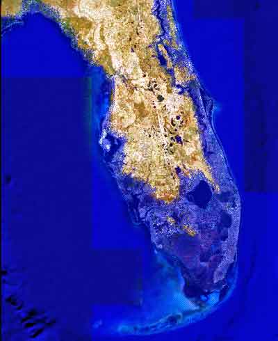
Image showing projected Florida flooding, from flood.firetree.net, using Google Earth with NASA data. Image from flood.firetree.net, using Google Earth.
Surveyors, prepare to get your feet wet. Global warming is about to hit you in the job list. By 2050, a majority of U.S. coastal areas are likely to be threatened by 30 or more days of flooding each year. This according to a December report in Earth’s Future, a journal of the American Geophysical Union.
[Parenthetically, the next issue of Survey Scene, in May, will be written by an actual geodesist. Until then, you have to put up with GPS World’s editor in chief — by no means a surveyor. Patience.]
The study used data from National Oceanic and Atmospheric Administration (NOAA) tide gauges to show the annual rate of coastal floods has accelerated in recent years. These are now five to 10 times more likely today than 50 years ago — and getting worse.
Mitigation decisions could range from retreating further inland to coastal fortification or to a combination of “green” infrastructure using both natural resources such as dunes and wetland, along with “gray” man-made infrastructure such as sea walls and redesigned storm water systems. And that’s not even mentioning such basics as redrawing property lines. Any way you look at it, surveyors are going to be involved.
“As communities across the country become increasingly vulnerable to water inundation and flooding, effective risk management is going to become more heavily reliant on environmental data and analysis,” said Holly Bamford, NOAA acting assistant secretary for conservation and management.
The recent U.S. Hydro 2015 conference in National Harbor, Maryland — an area particularly called out for vulnerability to the oncoming floods — naturally found a lot to talk about in this and related areas of interest for surveyors, with session tracks including: Effects of Climate Change on our Oceans and Waterways; Coastal and Ocean Mapping Initiatives; Advances in Unmanned System Technology, and several more.
Some of the papers presented that GPS World found of interest, and hopes to present or encapsulate in some form in the near future, include:
Resolving Systematic GPS Interference from Aeronautical Distance Measuring Equipment during Mission-Critical Shallow Water Multibeam Surveys
GPS Water-Level Buoy for Hydropgraphic Survey Operations
Examining the Uncertainty Associated with the Establishmenbt of an Ellipsoid to Chart Datum Separation Surface Using GNSS Buoys
Comparison of Horizontal and Vertical Resolvable Resolution between Repetitive Multibeam Surveys Using Different Kinematic GNSS Methods.
And those just came from the poster sessions. In the technical sessions, Jack Riley from the NOAA Coast Survey’s Hydrographic Systems and Technology Program presented a GPS Buoy Water Level Uncertainty Case Study.
Data from on High
Since you can’t get at a coastline from all angles — with any degree of stability, that is — data from overhead, sometimes far overhead, proves invaluable. Such as that provided by aerial digital imagery, LiDAR, and increasingly, satellites.
Because digital aerial images are already in electronic form, they can quickly be processed and made available to users. Most of the special cameras in use nowadays provide direct georeferencing capability, which allows camera position and orientation to be determined automatically using GPS and inertial measurement equipment. An entire mini-industry has grown up around integrating aerial data with that taken from ground surveys.
Light detection and ranging (LiDAR), a remote sensing system, became available for commercial topographic mapping in 1993. An airborne laser scanning system paired with a kinematic GPS receiver and an inertial navigation system can calculate and produce a highly accurate spot elevation. It is possible to obtain point densities that would likely take months to collect using traditional ground survey methods. The National Geodetic Survey (NGS) is currently implementing LiDAR into their shoreline mapping production process.
Our Record So Far
Coverage of these salty issues has been sparse in GPS World and associated newsletters, but not entirely absent. In 2006, the May issue featured “GPS Buoys Nautical Measurement.”
In 2008, Richard Langley edited an Innovation column on “Tsunami Detection by GPS,” featuring work for which co-author Attila Komjathy eventually won a GPS World Leadership Award in 2013. And in 2010, Langley brought forth an Innovation column on “Monitoring Water Level with GNSS.”
And way, way back in 2005, we published “Abreast of the Waves: Open-Sea Sensor to Measure Height and Direction.” This was prior to our digital era, so until we can scan a paper copy into here, we’ll simply give the abstract: “Accurate and timely information on open-sea wave conditions can help in preventing large-scale maritime disasters. This article describes a new, low-cost Global Positioning System (GPS)-based sensor that measures wave height with an accuracy of several centimeters and direction with an accuracy of 5 degrees. The receiver is mounted on a buoy, and a high-pass filter is used to extract the movement of the buoy and thus minimize GPS positioning errors. The data provided by the sensor is intended to improve wave prediction models. In addition, since this GPS-based sensor transmits only analyzed ocean wave data, it reduces the volume of data and leads to lower operating and acquisition costs. The article describes the concept of the GPS-based wave sensor, algorithms that are used for filtering and extracting wave data, as well as the results of open-sea trials.”
So there’s more to come. Watch this space. In the meantime, we leave you with Bob Dylan’s prophetic words, circa 1967.
Well, it’s sugar for sugar And salt for salt If you go down in the flood It’s gonna be your own fault.
A new report by Beecham Research examines how the agricultural sector is embracing precision farming to face challenges raised by an increasing worldwide population and the impact of climate change.
The United Nations predicts the global population will reach 8 billion by 2025, and 9.6 billion by 2050, meaning food production must increase by 70 percent by 2050.
The report explores how agricultural operations are changing through the Internet of Things (IoT) and related smart and connected farms concepts, including precision agriculture guided by GPS. It provides a geographic analysis discussing public policies, adoption drivers and barriers, and opportunities for the M2M/IoT community.
The Executive Summary of the report, “Towards Smart Farming: Agriculture Embracing the IoT Vision,” is available here.
The U.S. president’s fiscal year 2016 budget request for the U.S. Geological Survey (USGS) is $1.2 billion, an increase of nearly $150 million above the FY 2015 enacted level. According to a statement from the USGS, the FY16 budget “reflects the vital role the USGS plays in advancing the president’s ongoing commitment to scientific discovery and innovation to support a robust economy, sustainable economic growth, natural resource management, and science-based decision-making for critical societal needs.”
The budget request includes increases that ensure the USGS is at the leading edge of earth sciences research,” the statement continued. “It includes robust funding for science to inform land and resource management decisions, advance a landscape-level understanding of ecosystems, and develop new information and strategies to support communities in responding to climate change, historic drought, water quality issues, and natural hazards. The budget also funds science to support the nation’s energy strategy, to help identify critical mineral resources, and to address the impacts of energy and mineral development on the environment.”
“The USGS has a strong 136-year legacy of providing reliable science to decision-makers,” said Suzette Kimball, acting USGS director. “This budget request recognizes our unique capabilities with multi-disciplinary earth science research and will allow the USGS to meet societal needs for our nation now and in the future.”
Below are breakdowns of how the budget will address particular areas, according to the USGS.
Meeting Water Challenges in the 21st Century
The FY16 budget provides an increase of $14.5 million above the FY 2015 enacted level for science to support sustainable water management. Meeting the nation’s water resource needs poses increasing challenges for resource managers, who must contend with changes in the frequency and magnitude of floods and droughts. As competition for water resources grows for activities such as farming, energy production, and community water supplies, so does the need for information and tools to aid decision-makers. The budget provides increased funding across several USGS mission areas to support resource managers in understanding and managing competing demands related to water availability and quality and to enable adaptive management of watersheds to support the resilience of the communities and ecosystems that depend on them. This includes a $3.2 million increase for science to understand and respond to drought, a $4 million increase for water use information and research, a $2.5 million increase to study ecological water flows, a $1.3 million increase for stream flow information, and a $1.0 million increase to advance the National Groundwater Monitoring Network.
Powering Our Future and Supporting Sustainable Energy and Mineral Development
The 2016 USGS budget provides $9.6 million in program increases across the energy, minerals and environmental health portfolio for science to support the sustainable development of unconventional oil and gas resources, renewable energy sources such as geothermal, wind, and solar, critical minerals such as rare earth elements, and to address the environmental impacts of uranium mining.
Specifically, the budget includes a program increase of $1 million for mineral resources science to continue life-cycle analysis for critical minerals such as rare earth elements and to develop new science and tools to reduce the impacts of minerals extraction, production, and recycling on the global environment and human health. A life-cycle analysis will trace the flow of critical minerals from generation and occurrence through the consequences of human activity to ultimate disposition and disposal. The nation faces key economic decisions within each stage of the resource life cycle. Scientific understanding is an essential input to these decisions. The program change will support new workforce capability to address the main thrusts of the president’s four working groups in the Office of Science and Technology Policy that are currently focused on critical and strategic materials essential to national security, economic vitality, and environmental protection.
Responding to Natural Hazards
The budget provides an increase of more than $6.6 million above the FY 2015 enacted level for natural hazard science. This includes an increase of $4.9 million to expand the Global Seismic Network used for worldwide earthquake monitoring, tsunami warning, and nuclear treaty verification monitoring and research in partnership with the Department of Energy and the Department of Defense. It also includes a $1.7 million increase to support space weather (solar flare) geomagnetic monitoring. The increase will also support the installation and operation of rapid-deployable streamgages and expand the library of flood-inundation maps to help manage flood response activities.The proposed increase will also support landslide, wildfire, and sinkhole response capabilities as well as provide disaster scenario planning products for emergency managers. Included in the request is funding to build on investments to continue development of an earthquake early warning system, with the goal of implementing a limited public warning system for the U.S. west coast by 2018, as well as continued investments in volcano monitoring networks and science.
Building a Landscape-Level Understanding of Our Resources
The budget includes $15.6 million to expand, enhance, and initiate ecosystem science activities to increase the understanding of the nation’s landscapes and how they work. This includes budget increases of $6.7 million in support of critical landscapes. Specifically it provides a $4.2 million increase for the Arctic, a $1 million increase to study sagebrush landscapes that provide habitat for survival of greater sage-grouse, and a $1.5 million increase that supports science for Puget Sound, Columbia River, and the upper Mississippi River.
USGS research will continue to support restoration of other priority ecosystems, such as Chesapeake Bay, Everglades, Great Lakes, California Bay Delta, and the Gulf Coast. The budget request also provides an increase of $2.2 million for research on invasive plants and animals that cause significant economic losses in the U.S. and transmit diseases to wildlife and people, and $1.6 million to study the decline of insects, birds, and mammals that pollinate agricultural and other plants. Finally, the budget increases funding by $5.1 million to support coastal resilience to hazards and adaptation to long-term change from sea-level rise and coastal erosion.
Foundations for Land Management
The president’s budget request includes an increase of $37.8 million to provide data and tools to help land and resource managers make informed decisions across the landscape and provide data and information to the public for use in a wide variety of applications. The budgets of USGS and NASA provide complementary funding to sustain the Landsat data stream, which is critical to understanding global landscapes. An increase of $24.3 million in the USGS budget supports the ground system portion of the Sustained Land Imaging Program, including funding for ground systems development for a Thermal Instrument Free Flyer, Landsat 9 (a rebuild of Landsat 8), and to receive data from internal partners. The increase also will enhance the accessibility and usability of data. Specifically, the budget includes a $4 million increase for Landsat science products for climate and resource assessments.
The budget provides increases for other foundational data and tools needed to support landscape-level understanding. For example, an increase of $3.7 million will expand three-dimensional elevation data collection using ifsar (interferometric synthetic aperture radar) for Alaska and lidar (light detection and ranging) elsewhere in the U.S. in response to growing needs for high-quality, high-resolution elevation data to improve aviation safety, to understand and mitigate the effects of coastal erosion, storms, and other hazards, and to support many other critical activities. A $1.8 million increase will enhance understanding of the benefits of the nation’s ecosystem services, and a $1.1 million increase for the Big Earth Data Initiative will make high-value data sets easier to discover, access and use. The accessibility and usability of these data are critical for land management, hazard mitigation, and building a landscape-level understanding of our resources.
Supporting Community Resilience in the Face of a Changing Climate
The USGS plays an important role in conducting research and developing information and tools to support communities in understanding, preparing for, and responding to the impacts of global change. The budget includes an increase of $32 million above the FY 2015 enacted level for science to support climate resilience and adaptation. Climate change requires the nation to prepare for more intense drought, heatwaves, wildfire, flooding, and sea level rise. These challenges are already impacting infrastructure, food and water supplies, and physical safety in communities across the nation.
Understanding potential impacts to communities, ecosystems, water, plant and animal species, and other resources is crucial to federal, state, tribal, local, and international partners as they develop adaptive and resilient strategies in response to climate change. The budget includes a $6.8 million increase in science for adaptation and resilience planning, an increase of $2.3 million for the USGS to provide interagency coordination of regional climate science activities across the nation, an increase of $8.7 million to support biological carbon sequestration, and an increase of $11 million for the USGS to support the community resilience toolkit, which is a web-based clearinghouse of data, tools, shared applications, and best practices for resource managers, decision-makers, and the public.
The GPS Reflections Group of University of Colorado-Boulder has been awarded the prestigious Prince Sultan Bin Abdulaziz International Creativity Prize for Water. The prize is awarded biannually to acknowledge innovative work that contributes to the sustainable availability of water and the alleviation of the global problem of water scarcity.
The awards will be presented in a ceremony in Riyadh, Saudi Arabia, on December 16, concurrently with the 6th International Conference on Water Resources and Arid Environments (ICWRAE 6), December 16-18, 2014.
Professors Kristine Larson and Eric Small developed a new method to measure water at the Earth’s surface. The research team discovered that standard geodetic GPS instruments are sensitive to hydrological influences. They subsequently developed a cost-effective technique, GPS Interferometric Reflectometry (GPS-IR), to measure soil moisture, snow depth, and vegetation water content around GPS antennas. GPS-IR has the advantage of relying on an existing GPS infrastructure installed by surveyors and geoscientists that covers an increasingly large portion of the global surface.
Larson and Small collaborated with scientists at the University Corporation for Atmospheric Research and the National Atmospheric and Oceanic Administration, also in Boulder.
The team uses the GPS-IR technique to analyze data streams from existing GPS networks in near real-time. Data from hundreds of operational GPS sites are downloaded and processed, yielding estimates of hydrologic variables within 24 hours.
Scientists and government agencies can access this information at the team’s web portal and use the data to improve monitoring and forecasting of hydrologic variables.
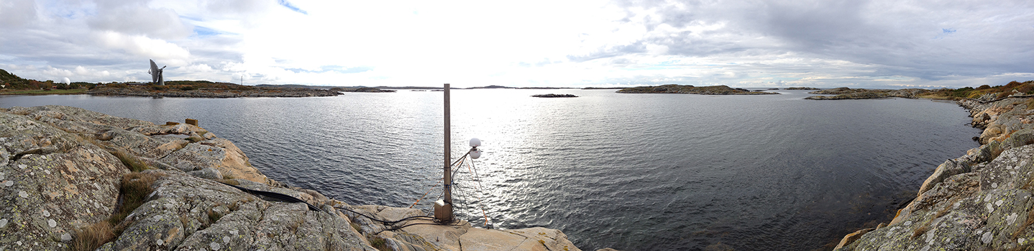
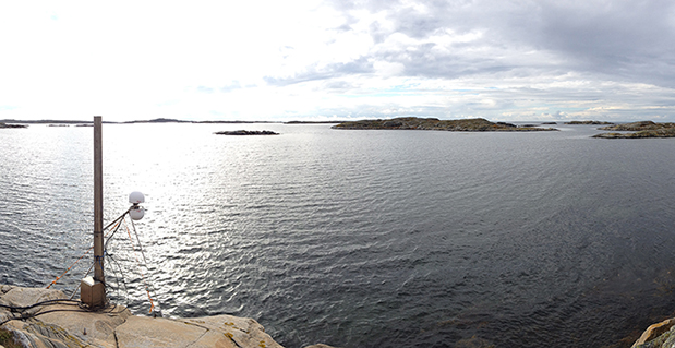
A panorama from the GNSS tide gauge at Onsala Space Observatory. When satellites pass over the sky, the GNSS tide gauge uses signals direct from the satellite and signals reflected off the sea surface to measure the sea level. Photo: Johan Löfgren
New Tide Gauge Uses GNSS to Measure Sea-Level Change
A new way of measuring and monitoring sea level — an important facet of researching climate change — has been implemented by scientists at Chalmers University of Technology in Sweden using existing coastal GPS stations.
When satellites pass over the sky, the GNSS tide gauge uses signals direct from the satellite and signals reflected off the sea surface to measure the sea level. Photo: Johan Löfgren
Measuring sea level is an increasingly important part of climate research, and a rising mean sea level is one of the most tangible consequences of climate change. Researchers at Chalmers University of Technology have studied new ways of measuring sea level that could become important tools for testing climate models and for investigating how the sea level along the world’s coasts is affected by climate change.
Johan Löfgren and Rüdiger Haas, scientists at Chalmers Department of Earth and Space Sciences, have developed and tested an instrument that measures the sea level using a GNSS tide gauge.
“The global mean sea level is rising because of climate change, but the change depends on where you are in the world,” said Rüdiger Haas. “We want to be able to make detailed measurements of sea level so that we can understand how coastal societies will be affected in the future.”
The GNSS tide gauge uses GPS and GLONASS signals. BeiDou and Galileo will be added in the future.
“We measure the sea level using the same radio signals that mobile phones and cars use in their satellite navigation systems,” said Johan Löfgren. “As the satellites pass over the sky, the instrument ‘sees’ their signals — both those that come direct and those that are reflected off the sea surface.”
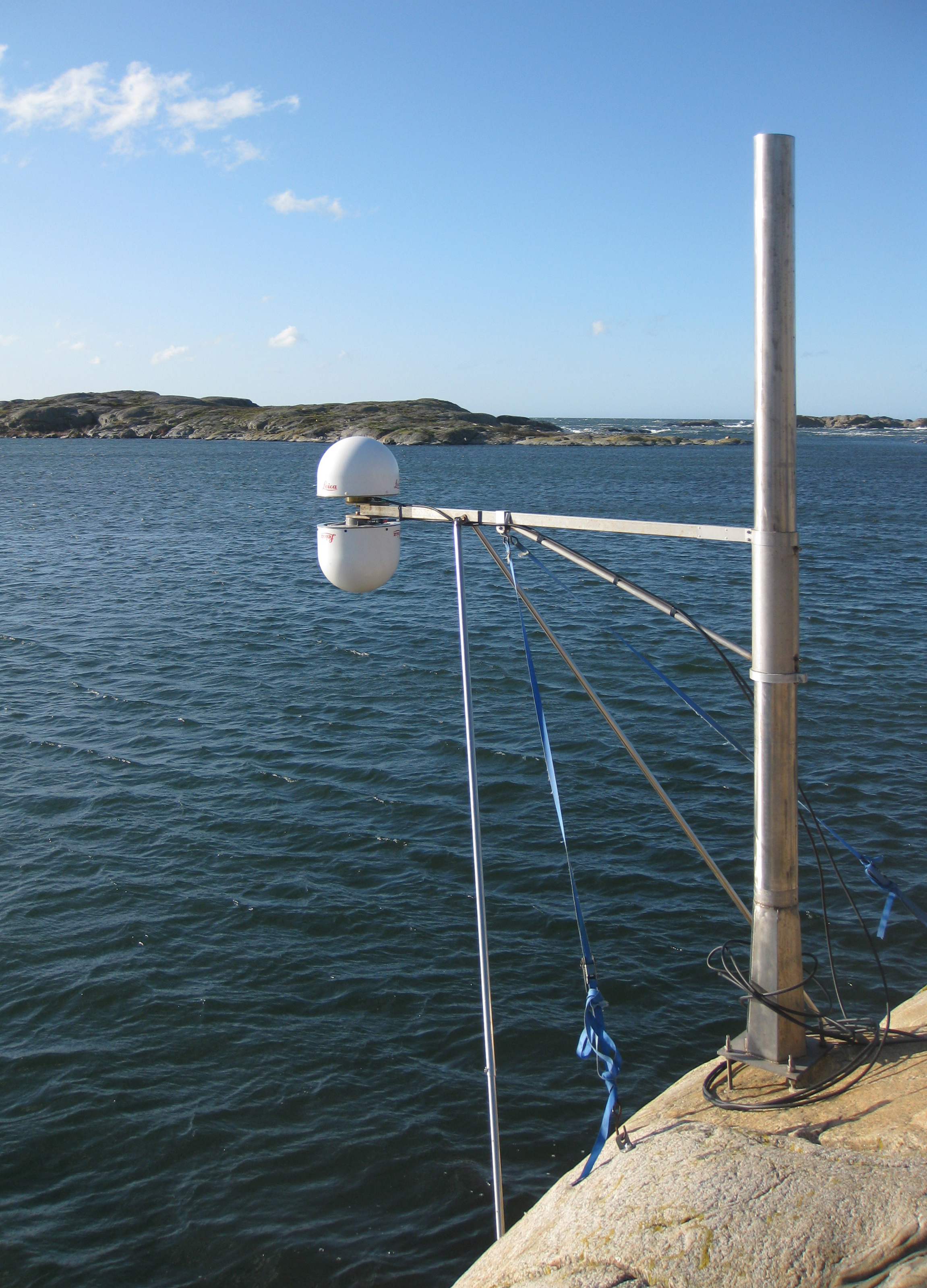
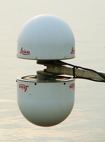
Antenna Setup. Two antennas, covered by small white radomes, measure signals both directly from the satellites and signals reflected off the sea surface. By analyzing these signals together, the sea level and its variation can be measured up to 20 times per second. The sea-level time series is rich in physical phenomena such as tides (caused mostly by the gravitational pull of the Moon and the Sun), meteorological signals (high and low pressure), and signals from climate change. Through advanced signal processing, these signals can be studied further.
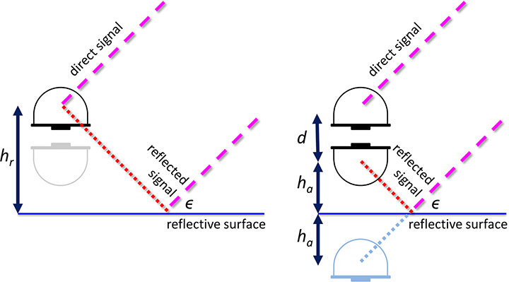
Schematic drawing of the GNSS tide gauge for SNR analysis (left) and phase-delay analysis (right). For the SNR analysis, the satellite signal with elevation ε reflects off the sea surface and interferes with the direct satellite signal at the antenna, creating an interference pattern in the recorded SNR observable that can be related to the reflector height, hr. For the phase delay analysis, the phase delays of the direct and the reflected signals are recorded separately, and through geodetic analysis of the phase delay, the baseline between the antennas can be determined and related to the height of the nadir-looking antenna over the sea surface, ha, and the vertical distance between the antenna phase centers, d.
The scientists’ initial study compared sea-level solutions from two analysis methods: signal-to-noise ratio (SNR) analysis and phase-delay analysis. The SNR analysis uses multipath signals observed with an upward-looking antenna, and the phase delay analysis uses the phase delay for both an upward- and a downward-looking antenna (see diagram).
Both GPS and GLONASS L1 and L2 signals were recorded, and the results were compared to independent measurements of sea level from a co-located pressure tide gauge. The GNSS-derived sea level showed a high correlation with the tide-gauge sea level for both analysis methods. Correlation coefficients for the phase-delay analysis and for the SNR analysis using frequency L1 were 0.95 to 0.97, whereas the correlation coefficients for the SNR analysis using frequency L2 were 0.86 to 0.87.
The phase-delay analysis shows a better agreement with the independent tide gauge sea level than the sea level from SNR analysis. Expressed as RMS differences, the phase-delay analysis achieves values of 3.5 cm (GPS) and 3.3 cm (GLONASS), whereas the SNR analysis achieves 4.0 cm (GPS) and 4.7 cm (GLONASS). The scientists concluded that, for the phase-delay analysis, it is possible to use both frequency bands, and for the SNR analysis, frequency band L2 should be avoided if other signals are available.
The GNSS tide gauge at Onsala Space Observatory uses signals from satellite navigation systems like GPS to measure the sea level. Photo: Johan Löfgren
Land and Sea. Unlike traditional tide gauges, the new GNSS tide gauge can measure changes in both land and sea at the same time, in the same location. That means both long-term and short-term land movements (post-glacial rebound and earthquakes) can be taken into consideration.
“Now we can measure the sea level both relative to the coast and relative to the center of the Earth, which means we can clearly tell the difference between changes in the water level and changes in the land,” said Johan Löfgren.
This summer, other high-precision instruments are being installed to work with the Onsala GNSS tide gauge, in collaboration with SMHI, the Swedish Meteorological and Hydrological Institute.
“Our tide gauge station will become part of a network of stations along the coast of Sweden that will be able to monitor changes in the water level to millimeter precision well into the future,” said Gunnar Elgered, professor at Chalmers Department of Earth and Space Sciences.
The scientists have also shown that existing coastal GNSS stations, installed primarily for the purpose of measuring land movements, can be used to make sea-level measurements.
“We’ve successfully tested a method where only one of the antennas is used to receive the radio signals. That means that existing coastal GNSS stations — there are hundreds of them all over the world — can also be used to measure the sea level,” said Johan Löfgren.
This work was previously reported in these publications: Larson, K.M., J. Lofgren, and R. Haas, “Coastal Sea Level Measurements Using A Single Geodetic GPS Receiver,” Adv. Space Res., Vol. 51(8), 1301-1310, 2013, doi:10.1016/j.asr.2012.04.017, 2013; and Larson, K.M., R. Ray, F. Nievinski, and J. Freymueller, “The Accidental Tide Gauge: A Case Study of GPS Reflections from Kachemak Bay, Alaska,” IEEE GRSL, Vol 10(5), 1200-1205, doi:10.1109/LGRS.2012.2236075, 2013.
Earth observing satellites are generating big data sets — Really Big!
I’m stepping in just for this month as a self-invited guest columnist, giving a brief look at the trailblazing work of the International Centre for Earth Simulation.
Look for both Eric Gakstatter and me at the ESRI User Conference in July, where Eric will also host a webinar on the hottest trends in mapping. We hope to accommodate a live audience at the webinar. If you’re not attending ESRI, attend the webinar anyway! For a top-level look at conference doings, register free.
In easily the most mind-blowing presentation of the Geospatial World Forum held recently in Geneva, Bob Bishop of the International Centre for Earth Simulation spun a vision of Big Data Earth Science, using the world’s largest computing resources (talk of exoflops and exobytes and “the human mind cannot comprehend these large volumes of data” supplied by many orbiting imagery satellites and other sensor inputs) to model the Whole Earth: surface, subsurface, ocean, atmosphere, and social economics.
The Centre’s mission is “Helping guide the successful transformation of human society in an era of rapid climate change and frequent natural disasters.”
In its prospectus, Bishop writes “The key to solving problems in weather, climate and environmental science is high-performance computing. Nature can only be accurately described and computed from equations that take account of complex, non-linear interactions between multiple natural systems, i.e. rivers, lakes, oceans, mountains, forests, dust, pollution, cloud cover, snow cover, ice, polar regions, etc. Such equations of motion are so interconnected and intertwined that they can only be managed when all aspects are held in big memory and computed simultaneously. Only then can we begin to address the systemic risks associated with natural disasters and planetary change.”
The ICES Foundation supports Open Science, which incorporates a combination of open data files, open source code, and open access publications. Much of the data supplied by the following organizations, upon whose resources ICES draws, is either directly produced by or referenced to GPS/GNSS data: Global Observing Systems Information Center and the U.S. National Oceanic and Atmospheric Adminisration; the European Space Agency and Centre for Space Records; the U.S. Geological Survey; the U.S. National Aeronautics and Space Administration; the European Union’s Joint Research Center; the U.S. National Center for Atmospheric Research; the U.S. Naval Research Laboratory; the European Commission’s Infrastructure for Spatial Information in the European Community (INSPIRE); and many more.
Slides from Bishop’s Geneva presentation are available here. These, however, of necessity lack some of the video and Flash Player simulations that he showed at the conference, revealing truly a dynamic planet in all aspects.
Bishop warned of both sequential and synchronous collapse of natural systems, leading to cascading crises. His language and message bear some resemblance to Al Gore’s An Inconvenient Truth, but Bishop, whose previous 40-year professional career had him responsible for building and operating the international aspects of Silicon Graphics Inc., Apollo Computer Inc., and Digital Equipment Corporation, has assembled some actual practical tools to apply to the many problems.
The immediate goal is modeling, simulation, visualization, and ultimately understanding of the whole, leading to new forms of civic engagement and insights as to risk, safety, food, water, and energy.
A panorama from the GNSS tide gauge at Onsala Space Observatory. When satellites pass over the sky, the GNSS tide gauge uses signals direct from the satellite and signals reflected off the sea surface to measure the sea level. Photo: Johan Löfgren
A new way of measuring sea level using satellite navigation system signals, for instance GPS, has been implemented by scientists at Chalmers University of Technology in Sweden. Sea level and its variation can easily be monitored using existing coastal GPS stations, the scientists have shown.
Measuring sea level is an increasingly important part of climate research, and a rising mean sea level is one of the most tangible consequences of climate change. Researchers at Chalmers University of Technology have studied new ways of measuring sea level that could become important tools for testing climate models and for investigating how the sea level along the world’s coasts is affected by climate change.
Johan Löfgren and Rüdiger Haas, scientists at Chalmers Department of Earth and Space Sciences, have developed and tested an instrument that measures the sea level using a GNSS tide gauge.
”The global mean sea level is rising because of climate change, but the change depends on where you are in the world,” says Rüdiger Haas. “We want to be able to make detailed measurements of sea level so that we can understand how coastal societies will be affected in the future.”
When satellites pass over the sky, the GNSS tide gauge uses signals direct from the satellite and signals reflected off the sea surface to measure the sea level. Photo: Johan Löfgren
The GNSS tide gauge uses GPS and GLONASS signals. BeiDou and Galileo will be added in the future.
”We measure the sea level using the same radio signals that mobile phones and cars use in their satellite navigation systems,” says Johan Löfgren. “As the satellites pass over the sky, the instrument ‘sees’ their signals — both those that come direct and those that are reflected off the sea surface.”
Two antennas, covered by small white radomes, measure signals both directly from the satellites and signals reflected off the sea surface. By analyzing these signals together, the sea level and its variation can be measured, up to 20 times per second. The sea level time series is rich in physical phenomena such as tides (caused mostly by the gravitational pull of the Moon and the Sun), meteorological signals (high and low pressure), and signals from climate change. Through advanced signal processing, these signals can be studied further.
The new GNSS tide gauge can measure changes in both land and sea at the same time, in the same location. That means both long-term and short-term land movements (post-glacial rebound and earthquakes) can be taken into consideration.
”Now we can measure the sea level both relative to the coast and relative to the center of the Earth, which means we can clearly tell the difference between changes in the water level and changes in the land,” says Johan Löfgren.
This summer, other high-precision instruments will be installed to work with the Onsala GNSS tide gauge, in collaboration with SMHI, the Swedish Meteorological and Hydrological Institute.
The GNSS tide gauge at Onsala Space Observatory uses signals from satellite navigation systems like GPS to measure the sea level. Photo: Johan Löfgren
”Our tide gauge station will become part of a network of stations along the coast of Sweden that will be able to monitor changes in the water level to millimeter precision well into the future,” says Gunnar Elgered, professor at Chalmers Department of Earth and Space Sciences.
The scientists have also shown that existing coastal GNSS stations, installed primarily for the purpose of measuring land movements, can be used to make sea-level measurements.
”We’ve successfully tested a method where only one of the antennas is used to receive the radio signals. That means that existing coastal GNSS stations — there are hundreds of them all over the world — can also be used to measure the sea level,” says Johan Löfgren.
More about the research
The method is described in two new scientific articles:
This work was previously reported in these publications:
Larson, K.M., J. Lofgren, and R. Haas, Coastal Sea Level Measurements Using A Single Geodetic GPS Receiver, Adv. Space Res., Vol. 51(8), 1301-1310, 2013, doi:10.1016/j.asr.2012.04.017, 2013.
Larson, K.M., R. Ray, F. Nievinski, and J. Freymueller, The Accidental Tide Gauge: A Case Study of GPS Reflections from Kachemak Bay, Alaska, IEEE GRSL, Vol 10(5), 1200-1205, doi:10.1109/LGRS.2012.2236075, 2013.
Esri announced that the Strauss Center’s Climate Change and African Political Stability (CCAPS) program has implemented Esri technology to view how climate change impacts vulnerable populations in Africa. CCAPS created the dynamic mapping tool in partnership with AidData for use by researchers, policy makers, journalists, and citizens. Users can visualize any combination of CCAPS data on climate change, conflict, and aid on a map to discover how different forces overlap or intersect.
“This mapping tool allows policy makers to analyze data from multiple sources at once, providing integrated analysis of the drivers and responses related to security risks stemming from climate change,” said Francis J. Gavin, director of the Strauss Center.
According to the announcement, the tool is already being used in the country of Malawi for a solution that tracks and reports on the country’s external funding. Aid information is mapped along with data on climate change vulnerability and incidents of conflict. This sheds light on whether aid is effectively targeting regions where climate change or conflict poses the most significant risk to the sustainable development and political stability of the country.
“Climate change poses an enormous threat to the livelihoods of millions of Africans,” said Jean-Louis Sarbib, CEO of Development Gateway. “The level of risk, however, is not evenly spread and certainly doesn’t respect national boundaries. To ask critical questions about how development assistance can reduce vulnerability, you need hyperlocal data on climate and also on aid-funded interventions. This is what the new CCAPS mapping tool shows in a digestible, interactive way.”
Esri reported that by integrating CCAPS research on climate change, along with existing datasets such as topographic maps, imagery, and thematic information on conflicts, the CCAPS mapping tool aims to provide the most comprehensive view possible of climate change and security in Africa.
“The great work of these organizations is a real game changer for the development community,” said Jack Dangermond, president of Esri. “Being able to create a tool that allows people to communicate with others all over the world using maps is powerful. I am impressed with the work being done and excited to see what they will think of next.”
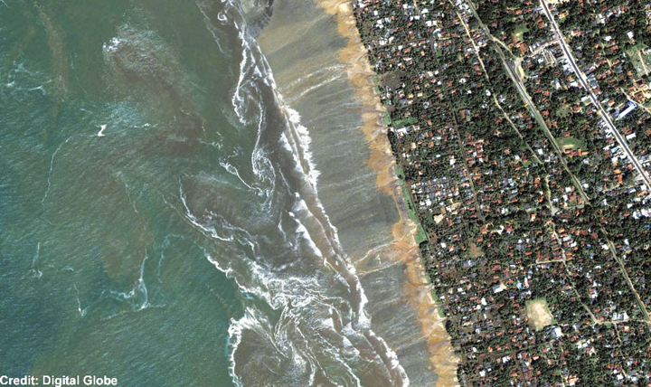
QuickBird satellite image of Kalutara Beach on the southwestern coast of Sri Lanka showing the receding waters and beach damage from the Sumatra tsunami.( Credit: Digital Globe)
How Ionospheric Observations Might Improve the Global Warning System
By Giovanni Occhipinti, Attila Komjathy, and Philippe Lognonné
Recent investigations have demonstrated that GPS might be an effective tool for improving the tsumani early-warning system through rapid determination of earthquake magnitude using data from GPS networks. A less obvious approach is to use the GPS data to look for the tsunami signature in the ionosphere.
INNOVATION INSIGHTS by Richard Langley
THE TSUNAMI generated by the December 26, 2004, earthquake just off the coast of the Indonesian island of Sumatra killed over 200,000 people. It was one of the worst natural disasters in recorded history. But it might have been largely averted if an adequate warning system had been in place.
A tsunami is generated when a large oceanic earthquake causes a rapid displacement of the ocean floor. The resulting ocean oscillations or waves, while only on the order of a few centimeters to tens of centimeters in the open ocean, can grow to be many meters even tens of meters when they reach shallow coastal areas. The speed of propagation of tsunami waves is slow enough, at about 600 to 700 kilometers per hour, that if they can be detected in the open ocean, there would be enough time to warn coastal communities of the approaching waves, giving people time to flee to higher ground.
Seismic instruments and models are used to predict a possible tsunami following an earthquake and ocean buoys and pressure sensors on the ocean bottom are used to detect the passage of tsunami waves. But globally, the density of such instrumentation is quite low and, coupled with the time lag needed to process the data to confirm a tsunami, an effective global tsunami warning system is not yet in place.
However, recent investigations have demonstrated that GPS might be a very effective tool for improving the warning system. This can be done, for example, through rapid determination of earthquake magnitude using data from existing GPS networks. And, incredible as it might seem, another approach is to use the GPS data to look for the tsunami signature in the ionosphere: the small displacement of the ocean surface displaces the atmosphere and makes it all the way to the ionosphere, causing measurable changes in ionospheric electron density.
In this month’s column, we look in detail at how a tsunami can affect the ionosphere and how GPS measurements of the effect might be used to improve the global tsunami warning system.
“Innovation” is a regular column that features discussions about recent advances in GPS technology and its applications as well as the fundamentals of GPS positioning. The column is coordinated by Richard Langley of the Department of Geodesy and Geomatics Engineering at the University of New Brunswick.
The December 26, 2004, earthquake-generated Sumatra tsunami caused enormous losses in life and property, even in locations relatively far away from the epicentral area. The losses would likely have never been so massive had an effective worldwide tsunami warning system been in place. A tsunami travels relatively slowly and it takes several hours for one to cross the Indian Ocean, for example. So a warning system should be able to detect a tsunami and provide an alert to coastal areas in its path. Among the strengths of a tsunami early-warning system would be its capability to provide an estimate of the magnitude and location of an earthquake. It should also confirm the amplitude of any associated tsunami, due to massive displacement of the ocean bottom, before it reaches populated areas. In the aftermath of the Sumatra tsunami, an important effort is underway to interconnect seismic networks and to provide early alarms quantifying the level of tsunami risk within 15 minutes of an earthquake.
However, the seismic estimation process cannot quantify the exact amplitude of a tsunami, and so the second step, that of tsunami confirmation, is still a challenge. The earthquake fault mechanism at the epicenter cannot fully explain the initiation of a tsunami as it is only approximated by the estimated seismic source. The fault slip is not transmitted linearly at the ocean bottom due to various factors including the effect of the bathymetry, the fault depth, and the local lithospheric properties as well as possible submarine landslides associated with the earthquake.
In the open ocean, detecting, characterizing, and imaging tsunami waves is still a challenge. The offshore vertical tsunami displacement (on the order of a few centimeters up to half a meter in the case of the Sumatra tsunami) is hidden in the natural ocean wave fluctuations, which can be several meters or more. In addition, the number of offshore instruments capable of tsunami measurements, such as tide gauges and buoys, is very limited. For example, there are only about 70 buoys in the whole world. As a tsunami propagates with a typical speed of 600–700 kilometers per hour, a 15-minute confirmation system would require a worldwide buoy network with a 150-kilometer spacing.
Satellite altimetry has recently proved capable of measuring the sea surface variation in the case of large tsunamis, including the December 2004 Sumatra event. However, satellites only supply a few snapshots along the sub-satellite tracks. Optical imaging of the shore hs successfully measured the wave arrival at the coastline (see ABOVE PHOTO), but it is ineffective in the open sea. At present, only ocean-bottom sensors and GPS buoy receivers supply measures of mid-ocean vertical displacement. In many cases, the tsunami can only be identified several hours after the seismic event due to the poor distribution of sensors. This delay is necessary for the tsunami to reach the buoys and for the signal to be recorded for a minimum of one wave period (a typical tsunami wave period is between 10 and 40 minutes) to be adequately filtered by removing the “noise” due to normal wave action.
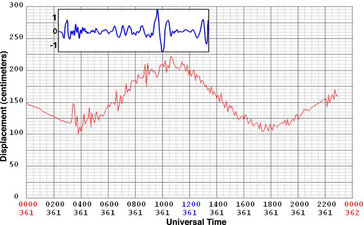
In the case of the December 2004 Sumatra event, the first tsunami measurements by any instrumentation were only made available about 3 hours after the earthquake. They were supplied by the real-time tide gauge at the Cocos Islands, an Australian territory in the southeast Indian Ocean (see FIGURE 1 where the tsunami signature is superimposed on the large semidiurnal tide fluctuation). Up until that time, the tsunami could not be fully confirmed and coastal areas remained vulnerable to tsunami damage. This delay in confirmation is a fundamental weakness of the existing tsunami warning systems.
Figure 1. The Sumatra tsunami signal measured at the Cocos Islands by the tide gauge (red) and by the co-located GPS receiver (blue). The tide gauge measures the sea-level displacement (tide plus superimposed tsunami) and the GPS receiver measures the slant total electron content perturbation (+/-1 TEC unit) in the ionosphere.
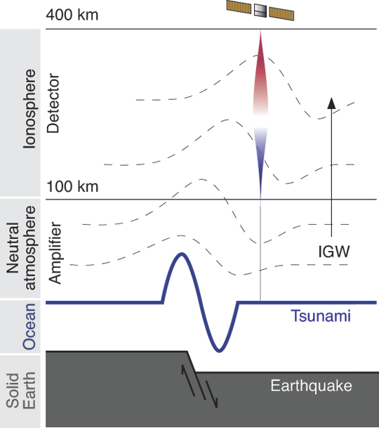
Ionospheric Perturbation. Recently, observational and modeling results have confirmed the existence and detectability of a tsunamigenic signature in the ionosphere. Physically, the displacement induced by tsunamis at the sea surface is transmitted into the atmosphere where it produces internal gravity waves (IGWs) propagating upward. (When a fluid or gas parcel is displaced at an interface, or internally, to a region with a different density, gravity restores the parcel toward equilibrium resulting in an oscillation about the equilibrium state; hence the term gravity wave.) The normal ocean surface variability has a typical high frequency (compared to tsunami waves) and does not transfer detectable energy into the atmosphere. In other words, the Earth’s atmosphere behaves as an “analog low-pass filter.” Only a tsunami produces propagating waves in the atmosphere. During the upward propagation, these waves are strongly amplified by the double effects of the conservation of kinetic energy and the decrease of atmospheric density resulting in a local displacement of several tens of meters per second at 300 kilometers altitude in the atmosphere. This displacement can reach a few hundred meters per second for the largest events.
At an altitude of about 300 kilometers, the neutral atmosphere is strongly coupled with the ionospheric plasma producing perturbations in the electron density. These perturbations are visible in GPS and satellite altimeter data since those signals have to transit the ionosphere. The dual-frequency signal emitted by GPS satellites can be processed to obtain the integral of electron density along the paths between the satellites and the receiver, the total electron content (TEC).
Within about 15 minutes, the waves generated at the sea surface reach ionospheric altitudes, creating measurable fluctuations in the ionospheric plasma and consequently in the TEC. This indirect method of tsunami detection should be helpful in ocean monitoring, allowing us to follow an oceanic wave from its generation to its propagation in the open ocean.
So, can ionospheric sounding provide a robust method of tsunami confirmation? It is our hope that in the future this technique can be incorporated into a tsunami early-warning system and complement the more traditional methods of detection including tide gauges and ocean buoys. Our research focuses on whether ground-based GPS TEC measurements combined with a numerical model of the tsunami-ionosphere coupling could be used to detect tsunamis robustly. Such a detection scheme depends on how the ionospheric signature is related to the amplitude of the sea surface displacement resulting from a tsunami. In the near future, the ionospheric monitoring of TEC perturbations might become an integral part of a tsunami warning system that could potentially make it much more effective due to the significantly increased area of coverage and timeliness of confirmation.
In this article, we’ll take a look at the current state of the art in modeling tsunami-generated ionospheric perturbations and the status of attempts to monitor those perturbations using GPS.
Some Background
Pioneering work by the Canadian atmospheric physicist Colin Hines in the 1970s suggested that tsunami-related IGWs in the atmosphere over the oceanic regions, while interacting with the ionospheric plasma, might produce signatures detectable by radio sounding.
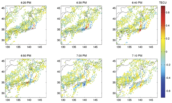
In June 2001, an episodic perturbation was observed following a tsunamigenic earthquake in Peru. After its propagation across the Pacific Ocean (taking about 22 hours), the tsunami reached the Japanese coast and its signature in the ionosphere was detected by the Japanese GPS dense network (GEONET). The perturbation, shown in FIGURE 2, has an arrival time and characteristic period consistent with the tsunami propagation determined from independent methods. Unfortunately, similar signatures in the ionosphere are also produced by IGWs associated with traveling ionospheric disturbances (TIDs), and are commonly observed in the TEC data. However, the known azimuth, arrival time, and structure of the tsunami allows us to use this data source, even if it contains background TIDs.
Figure 2. The observed signal for the June 23, 2001, tsunami (initiated offshore Peru). Total electron content variations are plotted at the ionosphere pierce points. A wave-like disturbance is seen propagating toward the coast of Honshu, the main island of Japan.
The December 26, 2004, Sumatra earthquake, with a magnitude of 9.3, was an order of magnitude larger than the Peru event and was the first earthquake and tsunami of magnitude larger than 9 of the so-called “human digital era,” comparable to the magnitude 9.5 Chilean earthquake of May 22, 1960.
In addition to seismic waves registered by global seismic networks, the Sumatra event produced infragravity waves (long-period wave motions with typical periods of 50 to 200 seconds) remotely observed from the island of Diego Garcia, perturbations in the magnetic field observed by the CHAMP satellite, and a series of ionospheric anomalies.
Two types of ionospheric anomaly were observed: anomalies of the first type, detected worldwide in the first few hours after the earthquake, were reported from north of Sumatra, in Europe, and in Japan. They are associated with the surface seismic waves that propagate around the world after an earthquake rupture (so-called Rayleigh waves).
Anomalies of the second type were detected above the ocean and were clearly associated with the tsunami. In the Indian Ocean, the occurrence times of TEC perturbations observed using ground-based GPS receivers and satellite altimeters were consistent with the observed tsunami propagation speed. The GPS observations from sites to the north of Sumatra show internal gravity waves most likely coupled with the tsunami or generated at the source and propagating independently in the atmosphere. The link with the tsunami is more evident in the observations elsewhere in the Indian Ocean. The TEC perturbations observed by the other ground-based GPS receivers moved horizontally with a velocity coherent with the tsunami propagation.
Figure 3. The tsunamigenic earthquake mechanism and transfer of energy in the neutral and ionized atmosphere. The solid Earth displacement produces the tsunami and the sea surface displacement produces an internal gravity wave in the neutral atmosphere, which perturbs the electron distribution in the ionosphere.
The amplitude of the observed TEC perturbations is strongly dependent on the filter method used. The four TECU-level peak-to-peak variations in filtered GPS TEC measurements from north of Sumatra are coherent with the differential TEC at the 0.4 TECU per 30 seconds level observed in the rest of the Indian Ocean. (One TEC unit or TECU is 1016 electrons per meter-squared, equivalent to 0.162 meters of range delay at the GPS L1 frequency.) Such magnitudes can be detected using GPS measurements since GPS phase observables are sensitive to TEC fluctuations at the 0.01 TECU level. We emphasize also the role of the elevation angle in the detection of tsunamigenic perturbations in the ionosphere. As a consequence of the integrated nature of TEC and the vertical structure of the tsunamigenic perturbation, low-elevation angle geometry is more sensitive to the tsunami signature in the GPS data, hence it is more visible.
The TEC perturbation observed at the Cocos Islands by GPS can be compared with the co-located tide-gauge (Figure 1). The tsunami signature in the data from the two different instruments shows a similar waveform, confirming the sensitivity of the ionospheric measurement to the tsunami structure.
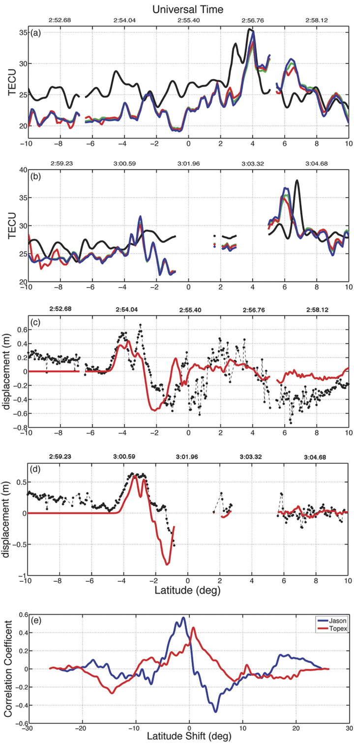
The link between the tsunami at sea level and the perturbation observed in the ionosphere has been demonstrated using a 3D numerical modeling based on the coupling between the ocean surface, the neutral atmosphere, and the ionosphere (see FIGURE 3). The modeling reproduced the TEC data with good agreement in amplitude as well as in the waveform shape, and quantified it by a cross-correlation (see FIGURE 4). The resulting shift of +/-1 degree showed the presence of zonal and meridional winds neglected in the modeling. The presence of the wind can, indeed, introduce a shift of 1 degree in latitude and 1.5 degrees in longitude.
Since modeling is an effective method to discriminate between the tsunami signature in the ionosphere and other potential perturbations, the GPS observations can be a useful tool to develop an inexpensive tsunami detection system based on the ionospheric sounding.
Figure 4. Satellite altimeter and total electron content (TEC) signatures of the Sumatra tsunami. The modeled and observed TEC is shown for (a) Jason-1 and for (b) Topex/Poseidon: data (black), synthetic TEC without production-recombination-diffusion effects (blue), with production-recombination (red), and production-recombination-diffusion (green). The Topex/Poseidon synthetic TEC has been shifted up by 2 TEC units. In (c) and (d), the altimetric measurements of the ocean surface (black) are plotted for the Jason-1 and Topex/Poseidon satellites, respectively. The synthetic ocean displacement, used as the source of internal gravity waves in the neutral atmosphere, is shown in red. In (e), the cross-correlations between TEC synthetics and data are shown for Jason-1 (blue) and Topex/Poseidon (red).
Modeling TEC Perturbations
A model to describe the effect of a tsunami on the ionosphere has been developed at the Institut de Physique du Globe de Paris (IPGP), France. It is comprised of three main parts. Firstly, it computes tsunami propagation using realistic bathymetry of, for example, the Indian Ocean. Secondly, an oceanic displacement is used to excite IGWs in the neutral atmosphere. Thirdly, it computes the response of the ionosphere induced by the neutral atmospheric motion resulting in enhanced electron densities. After integrating the electron densities, we obtain modeled (synthetic) TEC data. The modeling steps are as follows:
Tsunami Propagation. Tsunami modeling is an established science and the propagation of tsunamis is generally based on a shallow-water hypothesis. Under this hypothesis, the ocean is considered as a simple layer where the ocean depth, h, is locally taken into account in the tsunami propagation velocity, v = √ hg, which directly depends on h and the gravity acceleration g. The modeling, usually based on finite differences, solves the appropriate hydrodynamic equations.
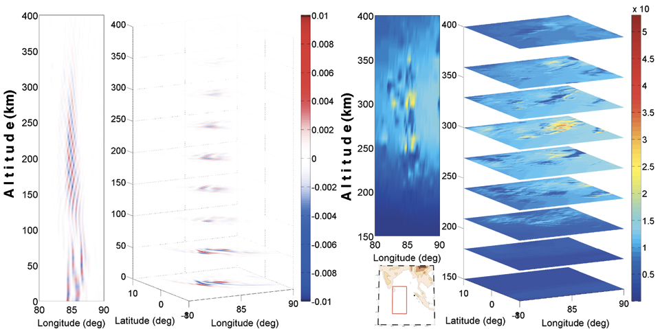
Neutral Atmosphere Coupling. A tsunami is an oceanic gravity wave and its propagation is not limited to the oceanic surface; as previously discussed, the ocean displacement is transferred to the atmosphere where it becomes an internal gravity wave. This coupling phenomenon is linear and can be reproduced solving the wave propagation equations, nominally the continuity and the so-called Navier-Stokes equations. These equations are solved assuming the atmosphere to be irrotational, inviscid, and incompressible. The IGWs are, indeed, imposed by displacement of the mass under the effect of the gravity force, contrary to the elastic waves generated by compression (for example, sound waves), so the medium can be considered incompressible. FIGURE 5 shows the IGWs produced by the Sumatra tsunami. The inversion of the velocity with altitude (wind shear) is a typical structure of IGWs.
Neutral-Plasma Coupling. The tsunamigenic IGWs are injected into a 3D ionospheric model to reproduce the induced electron density perturbations. In essence, the coupling model solves the hydromagnetic equations for three ion species (O2 + , NO+ , and O+ ). Physically, the neutral atmosphere motion induces fluctuations in the plasma velocity by way of momentum transfer driven by collision frequency and the Lorentz term associated with Earth’s magnetic and electric fields. Ion loss, recombination, and diffusion are also taken into account in the ion continuity equation. Finally, the perturbed electron density is inferred from ion densities using the charge neutrality hypothesis. The International Reference Ionosphere model is used for background electron density; SAMI2 (a recursive acronym: SAMI2 is Another Model of the Ionosphere) is used for collision, production, and loss parameters; and a constant geomagnetic field is assumed based on the International Geomagnetic Reference Field. FIGURE 5 shows the perturbation induced in the ionospheric plasma by the tsunamigenic IGW following the Sumatra event. The perturbation is strongly localized to around 300 kilometers altitude where the electron density background is maximized.
Figure 5. Internal gravity waves (IGWs) generated by the Sumatra tsunami and the response of the ionosphere to neutral motion at 02:40 UT (almost two hours after the earthquake). On the left, the normalized vertical velocity induced by tsunami-generated IGWs in the neutral atmosphere is shown. On the right, the perturbation induced by IGWs in the ionospheric plasma (in electrons per cubic meter) is shown, with the maximum perturbation at an altitude of about 300 kilometers. The vertical cut shown in these profiles is at a latitude of -1 degree.
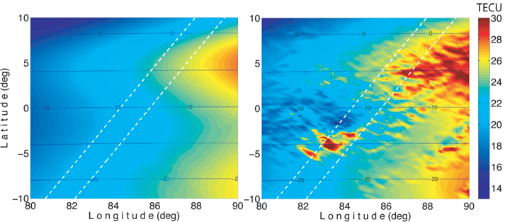
The resulting electron density dynamic model described above allows us to compute a map of the perturbed TEC by simple vertical integration (see FIGURE 6). In addition to the geometrical dispersion of the tsunami, the TEC map shows horizontal heterogeneities in the electron density perturbation that are induced by the geomagnetic field inclination. The magnetic field plays a fundamental role in the neutral-plasma coupling, resulting in a strong amplification at the magnetic equator where the magnetic field is directed horizontally. The isolated perturbation appearing more to the south is probably induced by the full development of the IGW in the atmosphere. Recent work also explains this second perturbation as induced by the role of the magnetic field in the neutral-plasma coupling.
Figure 6. The signature of the Sumatra tsunami in total electron content (TEC) at 03:18 UT (right) compared with the unperturbed TEC (left). The TEC images have been computed by vertical integration of the perturbed and unperturbed electron density fields. The broken lines represent the Topex/Poseidon (left) and Jason-1 (right) trajectories. The blue contours represent the geomagnetic field inclination.
GPS Data Processing
To validate our model, we use ground-based GPS receivers to look for the ionospheric signal induced by tsunamis. Prior research has shown post-processed results detecting a tsunami-generated TEC signal using regional GPS networks such as GEONET in Japan (about 1,000 stations) or the Southern California Integrated GPS Network (about 200 stations). Those studies benefited from the very high density of GPS receivers in the regional networks, so that, for example, no forward modeling was needed to help initially identify the characteristics of the tsunami-generated signal.
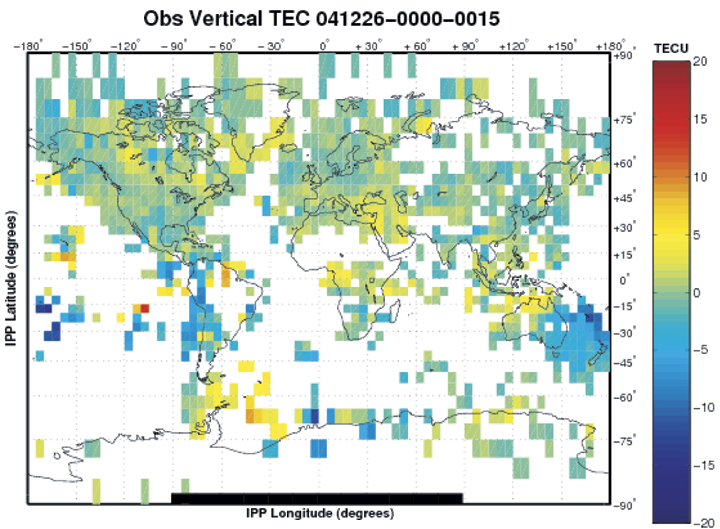
High-Precision Processing. More than 1,300 globally-distributed dual-frequency GPS receivers are available using publicly accessible networks, including those of the International GNSS Service and the Continuously Operating GPS Stations coordinated by the U.S. National Geodetic Survey. Most researchers estimate vertical ionospheric structure and, simultaneously, treat hardware-related biases as nuisance parameters. In our approach for calibrating GPS receiver and satellite inter-frequency biases, we take advantage of all available GPS receivers using a new processing technique based on the Global Ionospheric Mapping software developed at the Jet Propulsion Laboratory (JPL). FIGURE 7 shows a JPL TEC map using 1,000 GPS stations. This new capability is designed to estimate receiver biases for all stations in the global network. We solve for the instrumental biases by modeling the ionospheric delay and removing it from the observation.
Figure 7. The total electron content (TEC) between 01:00 and 01:15 UT on December 26, 2004, at ionosphere pierce points (IPPs) provided by a global network of more than 1,000 GPS tracking stations. To highlight variations, a five-day average of TEC has been subtracted from the observed TEC.
Ionospheric Warning System
The currently implemented tsunami warning system uses seismometers to detect earthquakes and to perform an estimation of the seismic moment by monitoring seismic waves. After a potential tsunami risk is determined, ocean buoy and pressure sensors have to confirm the tsunami risk. Unfortunately, the number of available ocean buoys is limited to about 70 over the whole planet. With the existing system, it may take several hours to confirm a tsunami when taking into account both the propagation time (of tsunamis reaching buoys) and data-processing time. On the other hand, the proposed ionosphere-based tsunami detection system may only require the propagation time and data-processing delays of only up to about 15–30 minutes. GPS receivers are able to sound the ionosphere up to about 20 degrees away from the receiver location, and a dense GPS network can therefore increase the coverage of the monitored area.
The fundamental idea behind a detection method is that we need to separate tsunami-generated TEC signatures from other sources of ionospheric disturbances. However, the tsunami-generated TEC perturbations are distinguishable because they are tied to the propagation characteristics of the tsunami. Tsunami-related fluctuations should be in the gravity-wave period domain and cohere in geometry and distance with the earthquake epicenter (for example, they show up in data on multiple satellites from multiple stations and, with increasing distance from the epicenter, at a rate related to tsunami propagation speed).
The coupled tsunami model described earlier can also be used to compute a prediction for the tsunami-generated TEC perturbation based on the seismic displacement as an input parameter to the model. The model prediction may be used as a detection aid by indicating the location of the tsunami wave front with time. This permits us to focus our detection efforts on specific locations and times, and will allow us to discriminate signal from noise.
The model also provides information on the expected magnitude of the TEC perturbation. This provides further value in filter discrimination. Cross-correlations can be performed on nearby observations using different satellites and stations to take advantage of tsunami-related perturbations being coherent in geometry and distance from the epicenter. Once the signal is detected in data from multiple satellites and stations, we can “track” and image the tsunami during its propagation in space and time.
The goal of our research is to assess the feasibility of detecting tsunamis in near real time. This requires that GPS data be acquired rapidly. Rapid availability of ground-based GPS data has been demonstrated via the NASA Global Differential GPS System, a highly accurate, robust real-time GPS monitoring and augmentation system.
Conclusions
Earlier research using GPS-derived TEC observations has revealed TEC perturbations induced by tsunamis. However, in our research, we use a combination of a coupled ionosphere-atmosphere-tsunami model with large GPS data sets. Ground-based GPS data are used to distinguish tsunami-generated TEC perturbations from background fluctuations. Tsunamis are among the most disrupting forces humankind faces. The December 26, 2004, earthquake and resulting tsunami claimed more than 200,000 lives, with several hundreds of thousands of people injured. The damage in infrastructure and other economic losses were estimated to be in the range of tens of billions of dollars. To help prevent such a global disaster from occurring again, we suggest that ionospheric sounding by GPS be integrated into the existing tsunami warning system as soon as possible.
Acknowledgments
This article is based on the paper “Three-Dimensional Waveform Modeling of Ionospheric Signature Induced by the 2004 Sumatra Tsunami” published in Geophysical Research Letters. The authors wish to acknowledge François Crespon (Noveltis, Ramonville-Saint-Agne, France) for the TEC data analysis in Figure 1, Juliette Artru (Centre National d’Etudes spatiales – CNES, Toulouse, France) for her work on the detection of tsunamigenic TEC perturbations shown in this article, and Grégoire Talon for Figure 3. The IPGP portion of the work is sponsored by L’Agence Nationale de la Recherche, by CNES, and by the Ministère de l’Enseignement supérieur et de la Recherche. The first author would also like to thank John LaBrecque of NASA’s Science Mission Directorate for supporting his fellowship at the California Institute of Technology/JPL.
GIOVANNI OCCHIPINTI received his Ph.D. at the Institut de Physique du Globe de Paris (IPGP) in 2006. In 2007, he joined NASA’s Jet Propulsion Laboratory (JPL), California Institute of Technology, as a postdoctoral fellow to continue his work on the detection and modeling of tsunamigenic perturbations in the ionosphere. He will soon take up the position of assistant professor at the University of Paris and IPGP. His scientific interests are focused on solid Earth-atmosphere-ionosphere coupling.
ATTILA KOMJATHY is senior staff member of the Ionospheric and Atmospheric Remote Sensing Group of Tracking Systems and Applications Section at JPL, specializing in remote sensing techniques. He received his Ph.D. from the Department of Geodesy and Geomatics Engineering at the University of New Bruns-wick, Canada, in 1997. He has received the Canadian Governor General’s Gold Medal for Academic Excellence and NASA awards including an Exceptional Space Act Award.
PHILIPPE LOGNONNÉ is the director of the Space Department of IPGP, a professor at the University of Paris VII, and a junior member of the Institut Universitaire de France. His science interests are in the field of remote sensing and are related to the detection of seismic waves and tsunamis in the ionosphere. Also, he participates in several projects in planetary seismology.
FURTHER READING
Ionospheric Seismology
“3D Waveform Modeling of Ionospheric Signature Induced by the 2004 Sumatra Tsunami” by G. Occhipinti, P. Lognonné, E. Alam Kherani, and H. Hebert, in Geophysical Research Letters, Vol. 33, L20104, doi:10.1029/2006GL026865, 2006.
“Ground-based GPS Imaging of Ionospheric Post-seismic Signal” by P. Lognonné, J. Artru, R. Garcia, F. Crespon, V. Ducic, E. Jeansou, G. Occhipinti, J. Helbert, G. Moreaux, and P.E. Godet in Planetary and Space Science, Vol. 54, No. 5, April 2006, pp. 528–540.
“Tsunamis Detection in the Ionosphere” by J. Artru, P. Lognonné, G. Occhipinti, F. Crespon, R. Garcia, E. Jeansou, and M. Murakami in Space Research Today, Vol. 163, 2005, pp. 23–27.
“On the Possible Detection of Tsunamis by a Monitoring of the Ionosphere” by W.R. Peltier and C.O. Hines in Journal of Geophysical Research, Vol. 81, No. 12, 1976, pp. 1995–2000.
“Unusual Topside Ionospheric Density Response to the November 2003 Superstorm” by E. Yizengaw, M.B. Moldwin, A. Komjathy, and A.J. Mannucci in Journal of Geophysical Research, Vol. 111, A02308, doi:10.1029/2005JA011433, 2006.
“Automated Daily Processing of More than 1000 Ground-based GPS Receivers for Studying Intense Ionospheric Storms” by A. Komjathy, L. Sparks, B.D. Wilson, and A.J. Mannucci in Radio Science, Vol. 40, RS6006, doi:10.1029/2005RS003279, 2005.
“Space Weather: Monitoring the Ionosphere with GPS” by A. Coster, J. Foster, and P. Erickson in GPS World, Vol. 14, No. 5, May 2003, pp. 42–49.
“GPS, the Ionosphere, and the Solar Maximum” by R.B. Langley in GPS World, Vol. 11, No. 7, July 2000, pp. 44–49.