Thales has been awarded a contract by the Service Industriel de l’Aéronautique (SIAé), France’s military aircraft maintenance, repair and overhaul service, to supply stand-alone GPS receivers for the French Navy’s Lynx helicopters, which are currently being upgraded by the French defence procurement agency (DGA).
Thales’s GNSS 1000-S receiver relies on SAASM (Selective Availability Anti-Spoofing Module) technology to access military GPS encrypted signals. This technology also uses state-of-the-art signal processing offering extended satellite tracking capabilities in terms of precision, integrity, availability and jamming resistance in severe operational conditions.
This contract consolidates Thales’s European leadership in the field of military GPS receivers, which already equip FREMM multi-mission frigates, cruise missiles, Tiger helicopters, C-135 refuelling aircraft, Atlantique-2 marine patrol aircraft and Mirage 2000D fighters in service with the French armed forces, and the tanker aircraft being delivered for the UK’s FSTA (Future Strategic Tanker Aircraft) programme.
The GNSS 1000-S is part of Thales’s suite of GNSS products which will be presented at the European Navigation Conference in Gdansk, Poland, April 25-27 on the Galileo Services booth.
As the GNSS world starts to appreciate the era of multiple global constellations, it’s probably worth considering the impact on aircraft navigation, GNSS airborne receivers and what these changes might soon bring to those who develop and use GNSS for airborne en-route navigation and approaches. Design and manufacture of new breeds of receivers are only the first of many steps along the road to full-fledged use of new capabilities. In aviation in particular, and in other high-precision fields to a lesser extent, many stages of study, regulation, development, test, and certification must be undertaken to eventually reach the promised land. The following capsule history of our progress to date also sheds light on what we may have to undertake in the future.
When GPS first came along, it was seen as a godsend for aviation. We’d been struggling with long-range Omega, which gave us, wow, close to a mile accuracy, and trying to get affordable but highly accurate Dopplers out of the military world. And those expensive inertials which still drifted pretty fast. GPS let us get to meters of position accuracy, was affordable, and could be used together with inertials to give us both bounded long-term accuracy and inertial azimuth, elevation and roll. Autopilots loved this stuff!
But, hey, when you put electronics onto an aircraft, you need standards and you need regulations. The International Civil Aviation Organization (ICAO), to which virtually all air-faring nations subscribe, sets up international standards for airborne system performance. ICAO quickly understood that GPS would be the navigation system that the whole world would come to rely on. So we got top-level marching orders from ICAO that set out the basic performance that we should expect from an airborne GPS system — Minimum Aviation System Performance Standards (MASPS).
The Federal Aviation Administration (FAA) in the U.S. as the world’s leading aviation agency took up the challenge and turned to the Radio Technical Commission for Aeronautics (a volunteer organization that develops technical guidance for use by government regulatory authorities and by industry — RTCA) to put together the Minimum Operational Performance Standards (MOPS). MOPS provide standards for specific equipment(s) used by designers, manufacturers, installers and users of the equipment. In fact, when we got MOPS for GPS, it allowed manufacturers of receivers and avionics to figure out what to build, what it should do, and how to qualify it. MOPS allowed the FAA to move on to develop the Technical Standard Order (TSO), which allowed FAA staff to verify compliance and ultimately install GPS avionics on aircraft via a Supplemental Type Certificate (STC) or, for new aircraft, via a Type Certificate. There are other ways onto aircraft too, but these are probably the most commonly used.
So we don’t just write our own specs and just develop and test it and sell it to aviation — there are a host of regulations you say…? That’s correct.
Around the same time GPS was hitting the streets, the FAA and other agencies recognized that these gizmos were basically software widgits, and that nerds could even be developing them in their garages or on their kitchen tables. We wrote software then that got the job done, and it worked at least as well as Microsoft’s did at the time, but our design and testing might have benefited from more structure. So along came RTCA DO-178 and subsequent revisions that set out the sequence of steps you should take to ensure a low probability of undetected error in your software. We started spending a whole lot more time upfront figuring out what the requirements were before we designed anything, and we had to wait what seemed like eons to get to code the stuff. So although we got process and we were able to cross-check between each step that we were still doing what we set out to do, the level and intensity of what came to be known as “verification” went through the roof. What a couple of guys in jeans had previously been able to cobble together in a couple of months now began to take a group of ten people working as an exceptionally well-coordinated team, maybe over several years. And the bright creative guys in the garages and kitchen tables were out of the aviation business. And a good proportion of the software engineers in the industry actually began to shun the rigor of the airborne software qualification/certification process, and prefer the less regimented receiver development associated with commercial receivers, especially challenging complex dual-frequency and RTK applications. So engineers with the persistence of airborne software qualification specialists are a rare and desired breed for airborne receiver manufacturers.
And then FAA put the same processes in place for hardware, especially ASICS, and gave us RTCA DO-254. Luckily we were already implementing ASICS using tools that applied thoroughness and intensity to the process, so DO-254 didn’t hurt quite as much as software development changes had hurt.
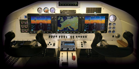
But we persevered, and eventually we got the bugs out of the receivers and got people flying with them, and there was great rejoicing in the aviation community. The General Aviation (GA) guys were a little impatient and couldn’t wait for the lengthy aviation development wheel to turn, so they bought handhelds in the meantime and duct-taped them to their yokes. But the FAA caught up with them, and these receivers evolved to the point where today they are buried behind square feet of glass Electronic Flight Instrument Systems (EFIS) and all you get is an icon which says your navigation source is GPS.
Avidyne Entegra Release 9 glass cockpit.
All these GPS receivers were, of course, single-frequency L1 only. Why, when there are perfectly good high-precision dual-frequency L1/L2 receivers out there? Well, turns out that only L1 is within the protected Aeronautical Radio Navigation Service (ARNS) band. The International Telecommunications Union (ITU) is an agency of the United Nations that manages worldwide allocation and use of radio frequencies — every country subscribes and plays by the ITU rules. So L1 is protected for GPS navigation use, but L2 isn’t. You can blast away with X-band radars in the L2 band and you’ll interfere with GPS L2 quite effectively. LightSquared assaults on the GPS bands excepted, the regulations currently protect you and your L1 GPS aviation receiver from intended and unintended jamming while your flight management system using GPS flies you safely from LaGuardia to Boston Logan.
So after several million dollars of engineering sweat and tears by receiver manufacturers, we eventually got ourselves to a point where we could fly GPS enroute from place to place, and the FAA even constructed and approved GPS approaches so we can get into airports. Then along comes WAAS, and we have new MOPS and new TSOs and many more millions of R&D required to implement WAAS LPV (Localizer Performance with Vertical guidance) approaches into the already certified L1 GPS receiver population. Crank up the machine and ensure each step is verified and the checks and balances of the aviation certification process ensure that we have the safety level needed to fly plane-loads of people through clouds and down to 200 feet with a half-mile visibility to the runway. It’s taken a lot of people a long time to work up these safety levels to use GPS like this, and guess what — it works!
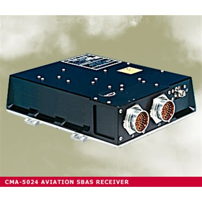
CMC airborne GPS receiver.
And Automatic Dependent Surveillance – Broadcast (ADS-B) is rolling out across the U.S. and other nations as we use GPS on-board aircraft to tell us where they are and to allow agencies to monitor air traffic with less radar tracking. Another leap in safety levels, which requires airborne receivers qualified to new MOPS.
Even though the accuracy might be there, the element we’ve struggled with all this time is integrity. And we get integrity by adding signals and ensuring there are always more signals than we have currently. So now we have L5 coming, and even Galileo and the prospect of multi-frequency, multi-constellation airborne receivers that add safety, raise integrity and get us closer to the runway on approach.
The FAA is mulling over the ground rules for the new L5 MOPS, which they would like to have done and receivers ready for when the next generation of WAAS is ready to go. Over in Europe, Eurocae (the European equivalent to RTCA in the U.S.) has already started to think about Galileo, and even L5. Over the coming years, as the U.S. GPS constellation adds L5 capability, maybe even at the same rate that Europe puts Galileo in place, aviation receiver manufacturers — a rare breed of specialists indeed — are trying to figure out how to finance the impending investments needed to make and certify this new generation of aviation receivers.
Some people have already started down this torturous development path, so they will be ready as the L5 and Galileo MOPS committees work through the intricacies of adding capability to the already highly structured spider’s web of regulations and requirements. As concepts are thought out, it’s always great to be able to test if they work on prototype hardware and provide validation back into the requirements process, so those who have working receivers will play a key role as these new capabilities are brought on line.
And let’s assume that Europe will want Galileo in its future aviation system, and that the pace of fielding L5 into the GPS constellation is unlikely to pick up given the economic restrictions under which the DoD will have to operate in the next few years.
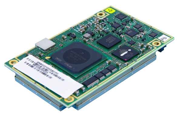
So, combined GPS L1/L5 Galileo E1/E5a receivers are favorite candidates for the next generation of airborne receivers. Rockwell Collins, Honeywell, CMC, Septentrio (at right, the Septentrio AiRx2 L1/L5 GPS E1/E5a airborne receiver), Accord, Garmin, and potentially others have their work cut out as we move out into a new generation of aviation satellite navigation capability. And yes, it’s very hard to do, folks.
The presence of different types of devices, spanning multiple GNSS receiver types, configurations, hardware, software, and consequent widely varying capabilites, among a user mix of vehicles, cyclists, and pedestrians, poses several engineering challenges for a V2X scheme in which all road users share data with each other and with the road infrastructure.
The use of location awareness for transportation safety, efficiency, and security — a major area of research and development for academics, automotive manufacturers, and organizations such as the U.S. Department of Transportation — has focused attention on enabling communication between vehicles and other road user entities in a concept know as V2X, a term encompassing both vehicle-to-vehicle (V2V) and vehicle-to-infrastructure (V2I) systems, so that they can share location and other status information. As a result, any road user entity may see all others around it. This capability is almost always built on GNSS technology.
Future V2X systems will be able to include all road user entities, ranging from vehicles to cyclists to pedestrians, in this information-sharing system. While it sounds natural for everyone to talk to each other and share data for collective benefit, the presence of different types of devices among this user mix poses several engineering challenges. As an example, a V2X device in a vehicle may have a built-in GNSS receiver with a roof-mounted antenna and another vehicle may have a retrofitted V2X device with a passive antenna and relatively limited accuracy capabilities. As the GNSS technology further develops, some vehicles may have multiple-frequency GNSS capability compared to legacy single-frequency devices. In essence, all compatible V2X devices will have to be carefully designed to ensure their interoperability with the rest of the system.
This article investigates positioning challenges arising from multiple GNSS receiver types, configurations, hardware, and software in a V2X operational environment. This produces a clear need to have minimum performance standards for V2X-capable GNSS receivers. The article further investigates the implications of land-based visibility obstructions on relative positioning, and implications on standalone position accuracy both as a result of limited GNSS satellite visibility and WAAS satellite visibility.
V2X Background
V2X systems rely on two critical enabling technologies: communications and positioning. Organizations and industry collaborations have developed and demonstrated various V2X systems over the last few years. These efforts have produced interoperable prototype V2V and V2I systems and over-the-air (OTA) messaging standards.
Figure 1 illustrates the general concept of combined V2V and V2I, or V2X. In a fully operational system, all vehicles and other road users carry short-range communication and positioning technology. At present, these technologies are expected to be based on dedicated short-range communication (DSRC) and GNSS, respectively. This enables each user to be location-aware and capable of sharing their location with others. Vehicles may use built-in systems, retrofitted devices, or those based on the occupant’s personal mobile device. Infrastructure elements and other road users such as pedestrians also form part of the V2X user community.
V2X Relative Positioning. Relative positioning of all communicating entities with respect to a given user is a required functional capability of a V2X system. To enable this functionality, positioning information from all communicating entities must be exchanged. For automotive V2X applications, Society of Automotive Engineers (SAE) J2735 DSRC Message Set Dictionary serves as the primary standard for message definitions. Current version of the messages consists of a basic safety message (BSM) , an optional variable rate message (VRM), and an option for including proprietary messages.
With BSM and VRM, vehicle position, speed, heading, and GNSS measurements can be communicated to others. GNSS relative positioning techniques such as real-time kinematic (RTK), code-based differential, or individual position differing (that is, distance between the positions reported by individual vehicles) can be used for relative positioning. The latter method, also known as DPOS, is a particular focus of this article.
Given the above, a system developer may develop a V2X relative positioning system that can operate based on techniques that can be broadly classified as position-based techniques, which include DPOS, and measurement-based differential techniques, including RTK and others.
The Simpler Approach. The SAE J2735 BSM accommodates the simpler approach of using the DPOS method, as it enables the sharing of critical state parameters. This approach is very attractive as it requires minimal OTA data volume compared to sending GNSS measurements. Secondly, DPOS relative position estimation process requires only a fraction of the processing resources required compared to measurement-based differential processing. Thirdly, any GNSS receiver in the market today is capable of outputting a position solution and most of the critical GNSS state parameters required for the V2X BSM. In contrast, most low-cost devices do not output measurements required for other methods.
However, there are quite a few challenges associated with DPOS. A vehicle or any other road-user entity, such as a location-enabled handheld device, will share its location information via BSM only. A relative positioning engine in each entity will use this information to provide lane-level and road-level data (relative distance, speed, and orientation) for its V2X applications. The challenges associated with DPOS method arise from multiple stages in this process.
The presence of many road-user types brings in the possibility of thousands of GNSS receiver types, models, hardware, and software in the user group. Thus the system must be interoperable with devices with a wide range of performance characteristics.
Secondly, each entity will transmit BSM only. This OTA information offers no information about the constellation the GNSS device sees or how the solution was derived in terms of filtering or applied constraints.
Thirdly, the position accuracy reported by each entity is a GNSS device-dependent variable, an estimate of the actual error as derived by a user device.
Finally and most importantly, V2X applications expect relative positioning information for each communicating entity classified in one of three possible accuracy categories: Which Road, Which Lane, or Where-in-Lane (see “Is GNSS up to the V2X Challenge?” GPS World, October 2010). The V2X system must be able to reliably identify this accuracy classification for each communicating entity with the limited information provided via the BSM.
Study Goals. To illustrate the impact of these challenges, several GNSS receiver types, configurations, and operational scenarios were investigated.
Between multiple receiver types: In a V2X environment, vehicles and other road user entities may have different GNSS receiver types and makes: dual-frequency, single-frequency, and so on.
Same receivers using different parts of visible constellation: In an urban canyon, it is possible for two adjacent vehicles to see two different parts of the GNSS constellation, due to obstructions.
WAAS-enabled and non-WAAS receivers.
Data Collection
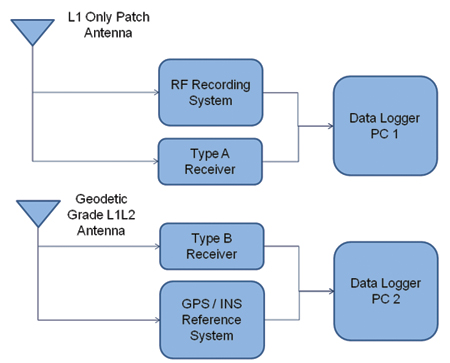
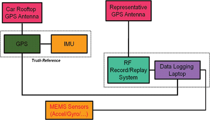
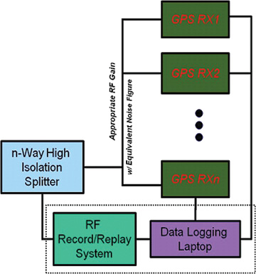
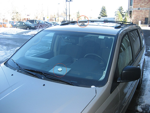
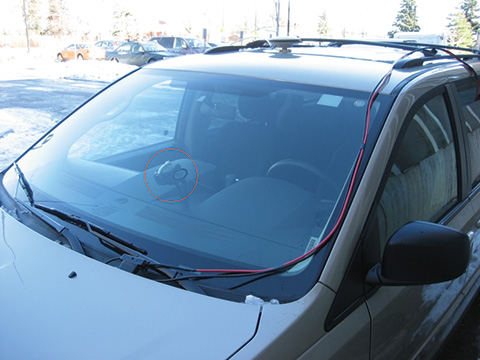
This data is a combination of field-data collections and a series of RF record playbacks. The field vehicle-mounted test setup included two GPS receivers, a GNSS L1 RF data recording device, and a high quality GPS/INS reference system (Figure 2). Type A receiver is a hi
gh-sensitivity enabled, automotive-grade GPS L1 receiver using a patch antenna, WAAS-capable although WAAS usage was disabled in the real-time data collection. Type B receiver is a high-quality L1/L2 receiver using a geodetic-grade antenna, used with WAAS enabled. The GPS/INS system was connected to the geodetic-grade antenna. The RF recording system was also connected to the automotive-grade GPS L1 antenna.
Figure 2. Vehicle test set-up.
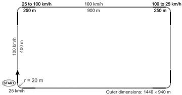
The data was collected on a test route in Detroit, Michigan, that included durations of urban and deep urban canyon (40 miles per hour (mph) or less), freeway (55–70 mph), and suburban/local (30 mph) driving.
The RF data were subsequently replayed to GNSS receivers that were not a part of the field set-up. RF data was also replayed to receivers with forced sky-visibility obstructions and various WAAS settings. For limited sky-visibility tests, certain satellites were removed from each receiver’s view by receiver-specific configuration software. The satellite selection and restriction was done to mimic typical sky-view obstructions encountered in normal driving.
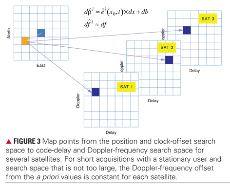
Type A receiver was chosen to illustrate the impact of visibility differences. A total of 13 satellites were visible in the entire data set (Figure 3). To create obstructed sky-view scenarios, two Type A receivers were configured to not use certain satellites in their position solutions. These configurations were:
Configuration 1 (C1): PRNs 7, 10, and 13 blocked
Configuration 2 (C2): PRNs 6, 16, 21, and 31 blocked
C1 mimics a vehicle/receiver with no visibility in the Northwestern part of the sky, whereas C2 mimics a receiver without visibility in the East/Northeastern part of the sky. Sky visibility restrictions do not vary with the heading changes of the vehicle. For example, for C1 receiver, Northwestern sky is always obstructed regardless of the vehicle orientation.
Figure 3. Sky view during the test.
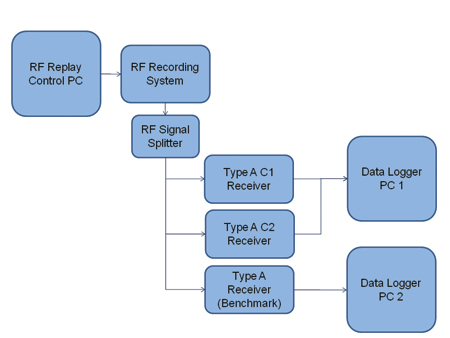
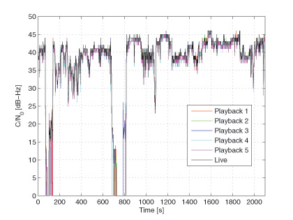
Figure 4 shows an example RF data replay setup. The record and replay system was controlled through a PC and the recorded data was also stored in the controller PC. The output RF signal was split into multiple outputs such that multiple receivers can be tested at the same time. For each replay of the RF data, a benchmark receiver was also used to verify that there is no run-to-run difference as a result of the RF replay.
Outputs from each GPS receiver from field and replay runs were logged to PCs using receiver specific binary formats. The recorded output from each receiver included its position, position error estimate, velocity, satellite-specific measurements and indicators such as pseudorange, carrier phase, and signals-to-noise ratio.
Figure 4. RF data replay set-up.
Data Processing and Analysis
The data was first decoded from the receiver-specific formats to a common format, then corrected for antenna offsets. To simplify the process, the reference system position solution was translated to the position of the test antenna using the known between-antenna distance and orientation of the vehicle as measured by the reference system. As a result, all the receivers and the reference system are reporting the location of the test antenna. Then, data fields such as position and velocity for each receiver were time-matched with the reference solutions, and the actual error was calculated.
For a limited dataset, additional measurement-level differential processing was done to show the difference between a DPOS and an RTK or a code-based differential relative position solution.
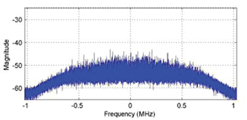
Figure 5 shows a plot of the 2D position error observed from each receiver during the test as a function of driving environment. Overall, Type B receiver shows better accuracy as expected from a dual frequency high quality receiver. However, it shows spikes of large error increases at times, mostly observed in the freeway scenario with large error excursions. With Type A receivers, relatively larger errors are observed with the limited-constellation receivers.
Figure 5. Position error (2D) of each receiver as a function of driving environment.
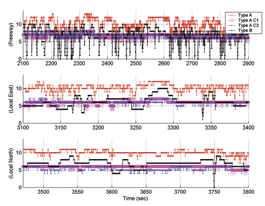
Figure 6 shows the number of satellites used by each receiver in the same environments as in Figure 5. Overall, Type A receiver tracks and uses on average 2–3 satellites more compared to the Type B receiver, likely due to its high-sensitivity capability. Type A C1 and C2 receivers also track and use 2–3 satellites fewer compared to the all-in-view Type A receiver.
Figure 6. GPS satellites used by receivers.
Freeway Data. The vehicle heading in this segment was predominantly north or northwest. The sky view can be considered a combination of urban and open sky conditions. As highlighted in Figure 6, all-in-view Type A receiver was able to use up to 11 GPS satellites with an average of around 9 satellites. Type A C1 and C2 receivers used, on average, about 3 satellites fewer than the all-in-view receiver. All three receivers show satellite count drops down to 4 at certain times in this segment.
The satellite count of the Type B receiver shows the limitations of not using the high-sensitive tracking capability. The satellite count shows frequent drops below 4 satellites and on occasion down to no satellites used.
Although the satellite count difference between all-in-view Type A and C1/C2 receivers was forced by means of receiver configuration, short-term sky visibility restrictions that resemble these conditions are in fact possible. Examples include a passenger car driving next to a semi truck or the side wall of the freeway in below-ground road sections.
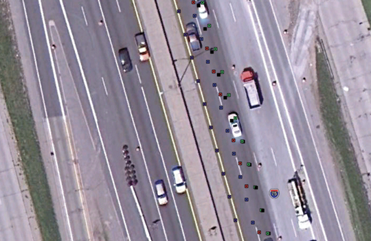
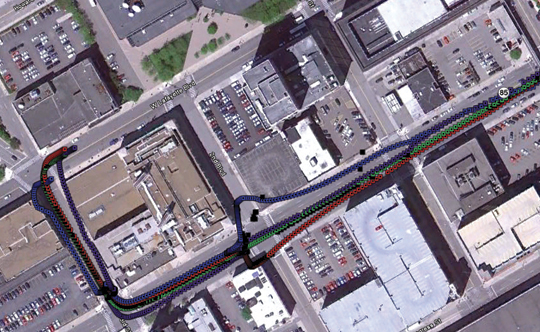
Figure 7 shows the position outputs of all four receivers on a satellite image of a short segment of the freeway. The true location (reference) is shown in green. Type A, Type B, Type A C1, and Type A C2 are shown in red, black, purple, and blue, respectively. These colors identify the four receiver types in all figures for the rest of this paper. While biases can be seen in the outputs of all four receivers with respect to the reference, the Type A C1 shows the largest offset with the magnitude of more than a lane width.
Figure 7. Freeway positioning accuracy.
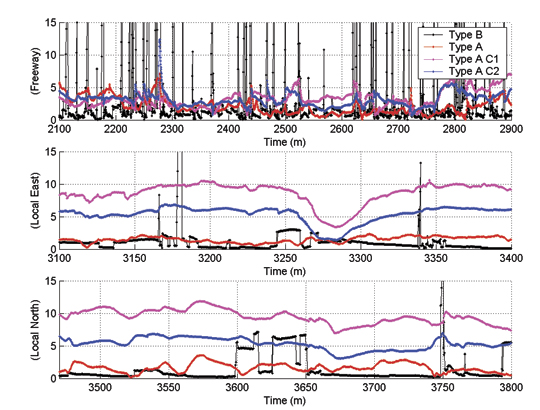
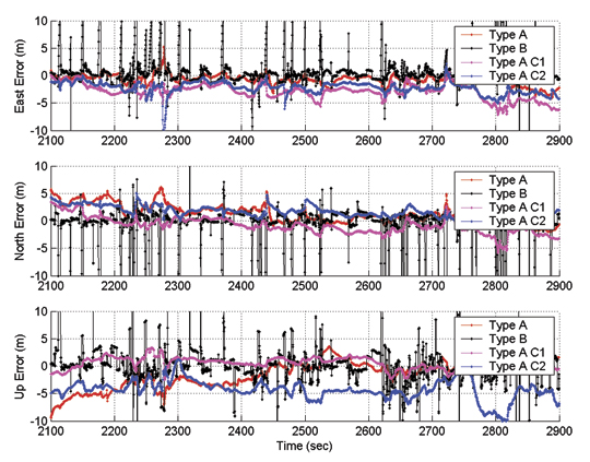
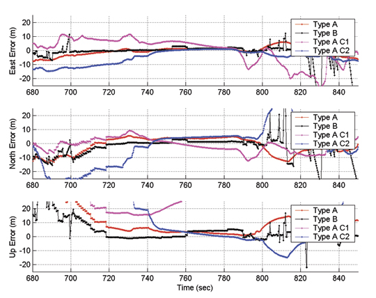
Figure 8 illustrates a time series of the positioning error components of all four receivers. It clearly shows error ramp-ups from the Type B receiver at frequent intervals. These coincide with the satellite count drops of Type B shown in Figure 6. No such error ramp-ups are observed for any of the Type A receivers, although relatively large biases of the order of few meters can be seen. As anticipated, larger errors are observed in the height direction.
Figure 8. Freeway positioning accuracy time series.
Local Road, Eastbound. This segment includes data gathered on an eastbound multi-lane local road with 40 mph posted speeds. As shown in Figure 6, a relatively larger number of satellites were continuously tracked in this segment as compared to the freeway. Therefore, this segment is considered to be an open-sky scenario with very limited number of obstructions. As shown in Figure 6, Type B receiver has used about 6 satellites on average, whereas the Type A has used around 3 more satellites most of the time. Type A C1 and C2 have also used around 3 satellites less compared to the all-in-view Type A receiver.
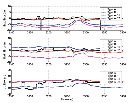
Figure 9 shows the vehicle position as reported by all three receivers and the reference system output for a short road segment in this drive. It clearly illustrates the lateral offsets of both C1 and C2 solutions. The C2 receiver (Blue) generated about a lane width offset towards north whereas the C1 receiver output is biased by around two lane widths to the south. Figure 10 presents a time series look of the positioning biases evident in Figure 9. It clearly shows large (more than 5 meter) biases in North and East position error components for C1 and C2 receivers.
Figure 9. Local (east) positioning accuracy.Figure 10. Local (east) positioning accuracy time series.
Local Road, Northbound. In roadway characteristics, this resembles Local Eastbound. Figure 6 shows the sky view remained almost unchanged for Type A receivers. For Type A C1, the count remained at 6 throughout. C1 and C2 receivers tracked 2–3 satellites fewer compared to all-in-view Type A. Interestingly, Type B experienced two dropouts of 4 or fewer satellites during the run. Figure 11 shows the position output of all receivers on a short road segment. As in the case of Local (East), significant biases can be readily observed in the output of C1 and C2.
Figure 11. Local (North) accuracy.
Figure 11. Local (North) accuracy.
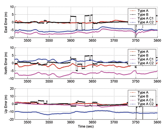
Figure 12 shows the time series view of the positioning error in this segment, confirming that the biases observed in Figure 11 are not short-term biases, but are in fact vehicle heading-dependent biases. The short-term biases seen in the Type B receiver output coincide with the change in the number of satellites used (shown in Figure 6). This illustrates the implications of different estimation methods used in the two receiver types. For instance, Type B receiver allows stepwise changes in its position estimate whereas Type A output tends to gradually converge to different states.
Figure 12. Local (North) positioning accuracy time series.
Urban Canyon. Results of the urban canyon segment of the drive are shown in Figures 13 and 14. A statistical analysis is not presented for this segment, as receiver type and configuration dependent biases and errors are difficult to isolate from the errors that are the result of multipath and measurement noise. In Figure 14, much larger biases in the order of 10 meters or more can be seen for all three Type A receivers. In comparison, Type B receiver tends to output a relatively accurate position solution whenever it has sufficient satellites visible. In the case of less than optimal satellites availability, Type B receivers tend to show rapidly degrading positioning accuracy, which may be reliably detected using its quality indicators.
Figure 13. Urban canyon accuracy.
Figure 14. Urban canyon positioning accuracy time series.
Position Error Distributions
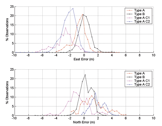
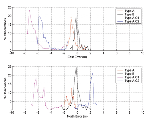
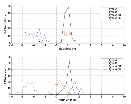
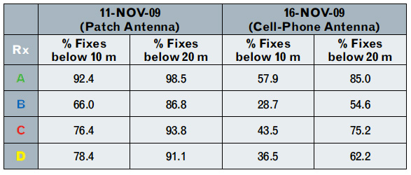
Position error probability distribution functions were generated for the first three road segments using the time series data above. Figures 15-17 show these functions for Freeway, Local (East), and Local (North) segments, respectively. They lead to these general conclusions:
Based on the mean and the spread of the distributions, Type B receiver has consistently provided the most unbiased and accurate positioning performance out of all the receivers considered. Overall, the output appears to be unbiased, as should be the case for a high quality dual frequency receiver with WAAS capability.
Type A all-in-view receiver shows the next best overall accuracy statistics with some biases in certain cases. These biases can be time-of-day-dependent and may differ for different times of the day or if observed over a longer time.
Type A C1 and C2 receivers show very significant vehicle-heading-dependent biases/errors. This is with very limited sky view obstructions (that is, C1 only restricts less than 1/8 of the entire sky view whereas C2 covers around 1/4) and with the same type of the receiver.
Although enabling WAAS should theoretically help minimize the biases observed in these tests, the availability (open line-of-sight) of WAAS satellites for automotive applications in these environments must be taken into consideration for WAAS accuracy benefits to be applicable. For these datasets, WAAS signals availabilities for a Type B receiver were 58 percent of total driving time in urban canyon, 60 percent in the freeway scenario, 95 percent and 99 percent in the local road scenarios.
Figure 15. Freeway position error distribution.Figure 16. Local road (east) position error distribution.Figure 17. Local road (north) position error distribution.
Velocity Domain Performance. For each test segment, velocity estimates from each receiver were logged at the default data rate of 4 Hz. For analysis purposes, North and East velocity readings from each receiver were converted to 2D speed estimates. These were used with reference system speed estimates to generate 2D speed error statistics (Table 1).
Based on Table 1, no significant biases or errors were observed from any particular receiver or configuration. The only exception was the increased errors in the Urban Canyon segment, particular for C1 and C2. This is expected .to be a result of limited satellite availability in a challenging environment with additional forced satellite eliminations.
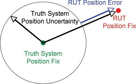
Virtual Two-Vehicle Analysis. Assume that Type A and Type A C1 receivers were located in two vehicles. Ideally, both receivers should report the same location, as they were both connected to the same antenna on a single vehicle, creating a zero-baseline scenario. However, as shown in the previous section, a meter-level separation was observed between the two solutions.
In this virtual two-vehicle scenario, relative position of one receiver (Type A) with respect to the other (Type A C2) was estimated by three methods, using GNSS data processing software in post-mission. The methods were:
Differenced Positions (DPOS). Latitude and longitude reported by each vehicle were time-matched; distance between the two points was calculated.
Code and Carrier. Single frequency (L1) GPS RTK positioning with float ambiguity estimation.
Code Only. GPS code measurements generated a relative position solution.
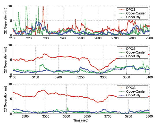
The 2D receiver separation results of this processing are shown in Figure 19 as three subplots for freeway (top), local/east (middle), and local/north (bottom) scenarios. The 2D separation results for local scenarios show clear performance benefits for the GNSS measurements-based methods. In both east and north local scenarios, around a 5-meter bias is observed in the DPOS solution whereas this is reduced to around a meter in both code-only and code and carrier methods. The freeway scenario shows relatively smaller difference potentially due to measurement noise, multipath, and frequent interruption of sky view. Table 2 shows mean values of these results.
Figure 18. Position separation for processing methods.Table 2. Mean Accuracy (meters) using processing methods.
Discussion
OTA transfer of certain GNSS measurement data elements appears to be a critical requirement for reliable lane-level positioning capability. However, the method must be capable of supporting a certain level of performance even in challenging environments for GNSS. The solution for such challenging environments is likely to be GNSS integration methods with vehicle-based sensors (that is, GNSS/INS) for the foreseeable future.
Given these facts, a reliable and accurate V2X relative position method will require the OTA transfer of a combination of critical vehicle states which include the vehicle location, a confidence measure, and certain GNSS measurement data elements. With its ability to support all of these needs, the SAE J2735 provides a basic framework for further refinement of relative positioning technologies for automotive applications.
A reliable position confidence measure broadcast over-the-air is also a critical need, particularly if GNSS measurement data is not broadcasted on a regular basis. This also holds true for conditions under which a vehicle may be operating in a GNSS and vehicle sensor integrated mode or with less than optimal number of satellites in view. However, estimating such a parameter that can be trusted with high degree of confidence can be challenging given the presence of various biases that can depend on the environment, vehicle, GNSS receiver, and sensors and methods used. Potential examples are time-of-day, vehicle heading, vehicle speed, GNSS receiver/sensor type, model, and configuration. However, developing a parameter similar to the RTCA Horizontal Uncertainty Level (HUL) for automotive applications is an important consideration.
While there are many other candidate receivers to be considered for a study of this nature, only two receiver types were used in this analysis. Analysis of more receiver types can be beneficial to identify the desired characteristics for a certain applications. A consideration could be achieving a desirable balance between accuracy and the sensitivity of the GNSS receivers, as increased sensitivity often produces higher solution availability at the cost of degrading accuracy.
Another area to investigate in related work is the benefits of using WAAS under the test conditions given in this paper. The general expectation is to see less bias in the position solution with WAAS as the ranging errors are likely to be smaller as a result of WAAS corrections. However, for automotive applications in particular, availability of WAAS signals to land vehicles need to be investigated.
CHAMINDA BASNYAKE is a senior research engineer at General Motors Global Research and Development and GNSS technology expert for GM OnStar. He leads GNSS-based vehicle navigation technology R&D efforts at GM and holds a Ph.D. in geomatics engineering from the University of Calgary.
By Cillian O’Driscoll, Gérard Lachapelle, and Mohamed Tamazin, University of Calgary
The impact of adding GLONASS to HS-GPS is assessed using a software receiver operating in an actual urban canyon environment. Results are compared with standard and high sensitivity GNSS receivers and show a significant improvement in the availability of position solutions when GLONASS is added. An assisted high sensitivity receiver architecture is introduced which enables high fidelity signal measurements even in degraded environments.
High-sensitivity (HS) GNSS receivers have flourished in the last decade. A variety of advances in signal-processing techniques and technologies have led to a thousandfold decrease in the minimum useable signal power, permitting use of GNSS, in particular GPS, in many environments where it was previously impossible.
Despite these recent advances, the issue of availability remains: in many scenarios there are simply too few satellites in view with detectable signals and a good geometry to compute a position solution. Of course, one way to improve this situation is to increase the number of satellites in view. GLONASS has been undergoing an accelerated revitalization program of late, such that there are currently more than 20 active GLONASS satellites on orbit. The combined use of GPS and GLONASS in a high-sensitivity receiver is a logical one, providing a near two-thirds increase in the number of satellites available for use.
The urban canyon environment is one in which the issue of signal availability is particularly important. The presence of large buildings leads to frequent shadowing of signals, which can only be overcome by increasing the number of satellites in the sky. Even if sufficient satellites are visible, the geometric dilution of precision can often be large, leading to large errors in position.
This work focuses on the advantages of using a combined GPS/GLONASS receiver in comparison to a GPS-only receiver in urban canyons. The target application is location-based services, so only single frequency (L1) operation is considered. We collected and assessed vehicular kinematic data in a typical North American urban canyon, using a commercially available high-sensitivity GPS-only receiver, a commercial survey-grade GPS/GLONASS receiver, and a state-of-the-art software receiver capable of processing both GPS and GLONASS in standard or high-sensitivity modes.
Processing Strategies
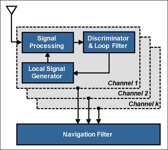
The standard (scalar-tracking) GNSS receiver architecture is shown in Figure 1. In the context of this article, the key characteristic of a standard receiver is that the signals from the different satellites are each tracked in parallel and independent tracking channels, and usually only three correlators are used. The information from the channels is only combined in the navigation filter to estimate position, velocity, and time. In this way, there is no sharing of information between channels in order to attempt to improve tracking performance.
Figure 1. Standard receiver architecture (courtesy Petovello et al).
Within each channel, the down-converted and filtered samples from the front end (not shown in Figure 1) are then passed to a signal-processing function where Doppler-removal (baseband mixing) and correlation (de-spreading) is performed. The correlator outputs are then passed to an error-determination function consisting of discriminators (typically one for code, frequency, and phase) and loop filters. The loop filters aim to remove noise from the discriminator outputs without affecting the desired signal. Finally, the local signal generators — whose output is used during Doppler removal and correlation — are updated using the loop-filter output.
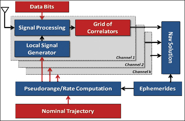
Assisted HS GNSS Receiver. The assisted HS GNSS receiver architecture used in this work is shown in Figure 2. Notable differences to the standard receiver architecture are highlighted in red.
Assistance information is provided in the form of broadcast ephemerides, raw data bits, and a nominal trajectory (position and velocity) that would normally be generated by the receiver. At each measurement epoch, the receiver uses the nominal position and velocity in conjunction with the ephemerides to compute the nominal pseudorange and pseudorange rate for each satellite in view. These parameters are passed to the signal-processing channels. Each channel evaluates a grid of correlators around the nominal pseudorange (code) and pseudorange rate (Doppler) values. The data bits are wiped off using the assistance information to permit long coherent integration times. For each signal tracked, the correlator grid is used to estimate code and Doppler offsets relative to the nominal values. These estimates are then used to generate accurate pseudorange and Doppler estimates.
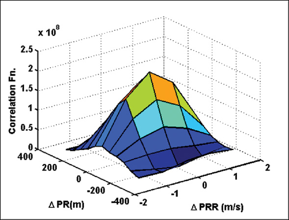
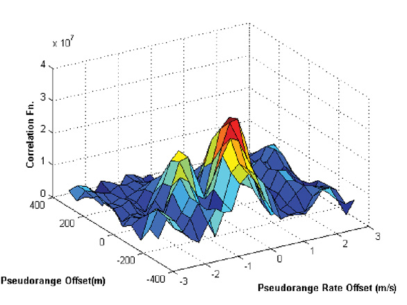
The number of correlators used and the spacing of these correlators in the code and frequency domains are completely configurable. A sample correlation grid computed during live data processing is illustrated in Figure 3. Measurements are generated by choosing the three correlators nearest the peak in the search space and using a quadratic fit to determine a better estimate of the peak location. In this work, a total of 55 correlators per channel were used.
Figure 3. Sample grid of correlator points computed for GPS PRN 04.
The assisted HS receiver is initialized in static mode in an open-sky setting during which reliable clock bias and drift estimates are derived. A high-quality oven-controlled crystal oscillator was used during this initial test to ensure that the clock drift did not change significantly over the period of the test (approximately 20 minutes). The clock bias during the test is updated using the clock drift estimate.
Note that this architecture is a generalization of the vector-based architecture, where the navigation solution used to aid the signal processing can be provided by an external reference.
Navigation Solution Processing. All navigation solution results presented here are obtained in single-point mode using an epoch-by-epoch least-squares solution with the PLAN Group C3NavG2 software, which uses both code and Doppler measurements. This processing strategy enables a fair comparison amongst the different signal processing strategies, as the smoothing effect of specific navigation filters is eliminated by this approach. More realistic accuracy estimates of the measured pseudoranges can be obtained. It is understood that in an operational environment, a well-tuned filter will obtain significantly better navigation performance than the epoch-by-epoch solutions presented here.
The measurements are weighted using a standard-elevation-dependent scheme. Thus there is no attempt to tune the weighting scheme for each receiver.
Data Collection
To test the relative performance of the various processing strategies, we conducted a test in downtown Calgary. Data was collected using a commercial HS GPS receiver, a commercial survey grade GPS/GLONASS receiver, and an RF downconverter and digitizer. The digitized data was post-processed in two modes (standard and assisted HS GNSS) using the PLAN group software receiver GSNRx.
Raw measurements were logged from each of the commercial receivers at a 1-second interval. The parameters used in GSNRx are given in Table 1.
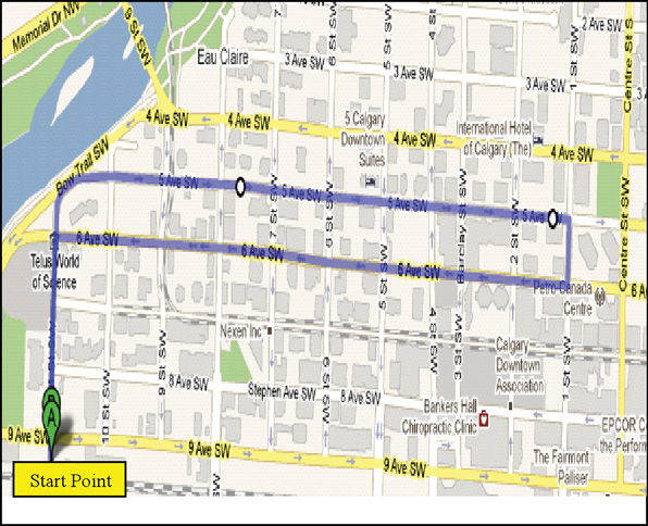
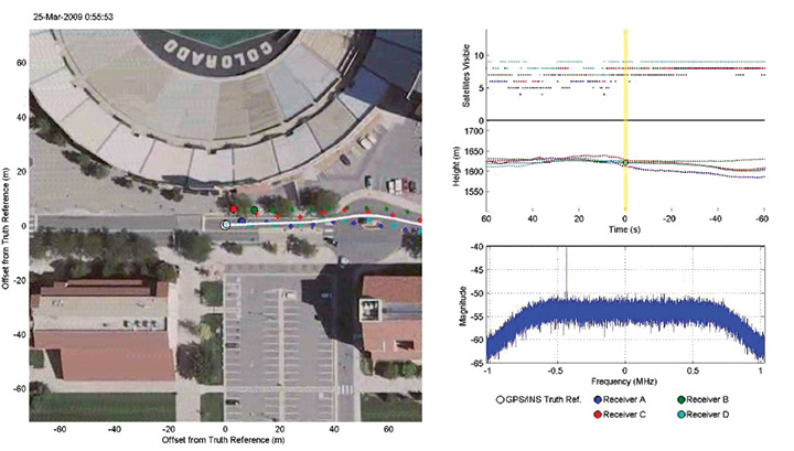
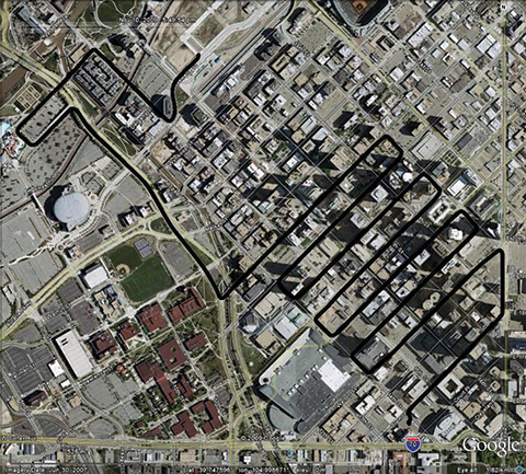
The trajectory followed is shown in Figure 4. The majority of the route was travelled in an East-West direction, with significant signal masking to the North and South. The Opening Photo shows an aerial view of downtown Calgary where the test took place. Masking angles exceeded 75 degrees along the vehicle trajectory.
Figure 4. Test Trajectory where the route is approximately 4 km with a 10 minute travel time.
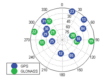
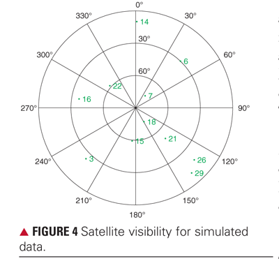
A sky plot of the satellites visible above a 5-degree elevation mask at the test location is shown in Figure 5. A total of 11 GPS and seven GLONASS satellites were present.
Figure 5. Skyplot of GPS and GLONASS satellites over Calgary at the start of the test.
A static period of approximately three minutes duration was used to initialize the assisted HS GNSS processing. During this period, the vehicle had a largely clear view of the sky. Nevertheless, three satellites were blocked from view during this period, namely GPS SVs 13 and 3, and GLONASS SV 22. As a result, these SVs were not available for processing in the assisted HS GNSS mode. The two commercial receivers were already up and running prior to the initialization period and so were able to process these three low-elevation satellites when they came into view during the test. See PHOTO on next page for a typical scene during the downtown test.
Analysis
To study the impact of adding GLONASS, the analysis focuses on solution availability, the number of satellites used in each solution, the DOP associated with each solution, and the statistics of the least-squares solution residuals. In the absence of a reference solution, the statistics of the residuals nevertheless give a reasonable indication of the quality of the measurements used, provided sufficient measurements are available to ensure redundancy in the solution. Nevertheless, some pseudorange errors will be absorbed by the navigation solution, hence the statistics of the residuals can be viewed as only a good estimate of the quality of the measurements themselves.
Solution Availability. As previously discussed, the navigation processing strategy adopted is the same for all receivers used in the test. A single-point epoch-by-epoch least-squares solution is computed at a 1 Hz rate. If there are insufficient satellites in view at a given epoch, or the solution fails to converge in 10 iterations, no solution is computed. In this section, the analysis focuses on the percentage of epochs during the downtown portion of the test for which a solution was computed.
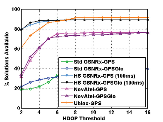
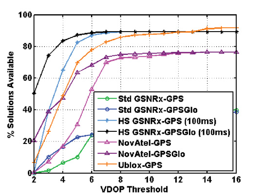
Figure 6 shows the percentage of solutions computed for each receiver processing strategy as a function of HDOP and VDOP thresholds, respectively. Thus, for example, the assisted HS GPS-GLONASS processing strategy yielded navigation solutions with a HDOP less than 6 between 80 percent and 85 percent of the time. For larger DOP thresholds, it is clear that there is little difference between GPS-only processing and GPS+GLONASS processing. The biggest differences are caused by the processing strategies employed. The advantages of HS processing are clear, at least in terms of solution availability. For this test and the particular geometry of the satellites in view during the test, GPS+GLONASS processing does yield a noticeable improvement in the VDOP, particularly at lower thresholds.
Figure 6A. Percentage solution availability versus HDOP threshold.Figure 6B. Percentage solution availability versus VDOP threshold.
Note that the standalone HS GPS receiver exhibits greater solution availability than the assisted software HS GPS-GLONASS receiver at higher DOP thresholds. This is most likely due to the low-elevation satellites that were excluded from the assisted HS processing due to their being masked during the initialization period as discussed earlier. Overall, however, there is little difference between GPS-only processing and GPS-GLONASS processing in terms of solution availability. This fact, of course, does not yield any information on the quality of the solutions obtained, which is discussed later.
To gain further insight into the impact of GLONASS, Figure 7 shows the percentage of solutions computed that exhibit redundancy. Thus, of all solutions computed during the downtown portion of the test, Figure 7 illustrates the percentage of those solutions that have redundant measurements. For GPS-only processing, this implies that five or more measurements were used in computing the position, while for GPS-GLONASS processing a minimum of six measurements were required. In this case, the advantage of using GLONASS becomes more apparent. For all processing strategies the addition of GLONASS yields an increase of 5 to 10 percent in the number of solutions with redundancy. Although not studied herein, this would have a positive impact on fault detection.
Residuals Analysis
To investigate the quality of the measurements generated by each processing strategy, the residuals from the least-squares solutions are studied. Only those epochs for which redundant solutions are computed are considered here, since non-redundant solutions lead to residuals with values of zero. As discussed above, the analysis of these residuals gives an estimate of the quality of the measurements generated.
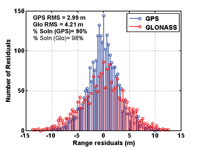
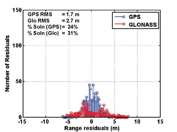
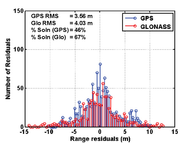
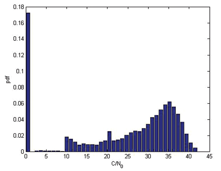
Figure 8 shows the histograms of the residuals from all GPS-GLONASS processing strategies. Once again, it is important to emphasize that only residuals from solutions with redundancy are considered. In addition, the results presented are limited to those epochs during which the vehicle was in the downtown portion of the test. For the purposes of this presentation an upper GDOP threshold of 10 was set.
It is interesting to note that in all cases (assisted HS, standard wide correlator, and commercial survey-grade processing), the relative RMS values of the GPS and GLONASS residuals are about the same. These results indicate that, irrespective of the signal-processing strategy employed, the GLONASS measurements are of a similar quality to the GPS measurements. The number of residuals available is however different between the standard and HS solutions, as the latter produce more measurements and more redundant solutions, hence more residuals. The processing strategy obviously had a significant impact on the availability of redundant solutions as discussed in the previous section.
Figure 8A. GPS-GLONASS range residuals comparison: assisted HS-GPS-GLONASS. RMS values and the percentage of solutions used in the histogram are also shown.Figure 8B. GPS-GLONASS range residuals comparison: standard wide correlator. RMS values and the percentage of solutions used in the histogram are also shown.Figure 8C. GPS-GLONASS range residuals comparison: survey-grade receiver. RMS values and the percentage of solutions used in the histogram are also shown.
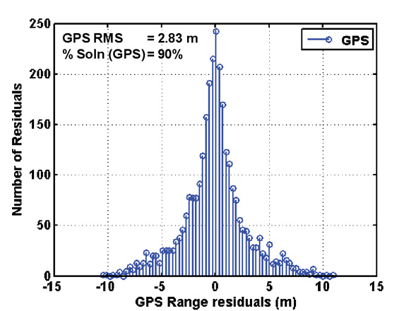
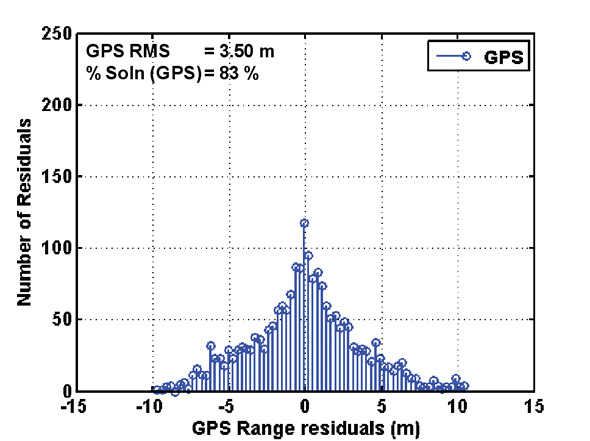
Figure 9 shows the histograms of the range residuals from GPS-only processing. In this case, the navigation solution is a GPS-only navigation solution, though in the case of the assisted HS receiver the measurements used are identical to those used in Figure 8.
Clearly the assisted HS receiver has a greater availability of redundant solutions compared to the standalone receiver, which is to be expected. Also, the assisted HS GPS receiver residuals have a slighter lower RMS than when a GPS-GLONASS implementation was considered, indicating that the navigation solution absorbs more of the measurement errors in this case.
Figure 9A. GPS range residuals comparison, assisted HS GPS.Figure 9B. GPS range residuals comparison, commercial standalone HS GPS.
Position Domain Results
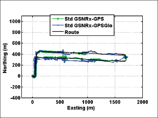
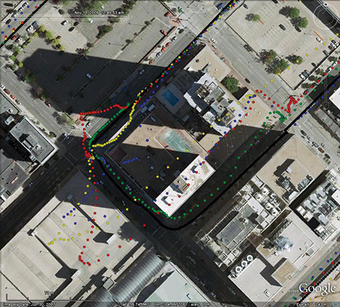
The final stage of the analysis is a comparison of the trajectories computed using each of the receiver types. While no truth solution was available for this test, a highly filtered navigation solution from the high-sensitivity commercial receiver was used as a nominal reference. This trajectory is shown in black in the following figures.
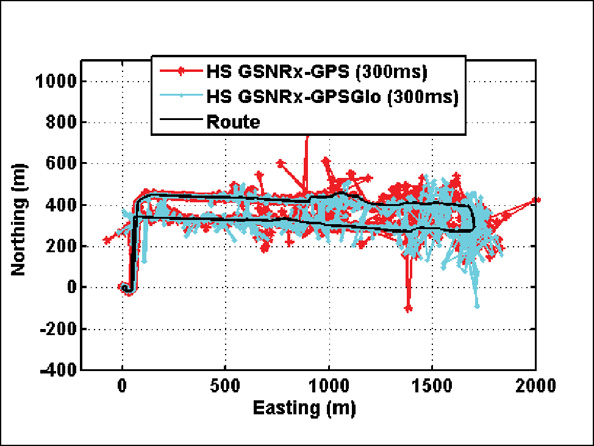
Figure 10 shows the trajectories obtained using standard wide-correlator processing. The position solutions are quite accurate, but the availability is low, namely of the order of 30 percent as shown above. The addition of GLONASS does improve the availability in this case. The accuracy is not significantly improved. In fact it appears that the addition of GLONASS occasionally leads to biases in the navigation solutions, likely solutions with high DOP values.
Figure 10. Trajectory obtained with standard wide correlator processing.
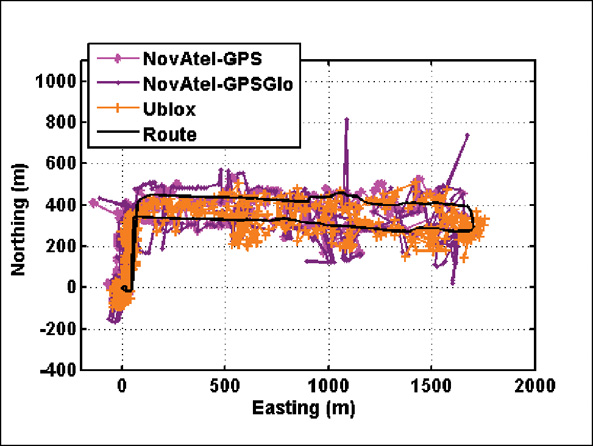
Figure 11 shows the trajectories computed using the commercial receivers. The survey-grade receiver yields less noisy positions, though the addition of GLONASS does lead to some significant outliers. The position availability is lower as discussed earlier. Similar to the standard wide-correlator processing case, the addition of GLONASS again appears to introduce an error in the solution during some epochs (for example, at a northing of about 500 meters between 100 and 500 meters easting).
Figure 11. Trajectories obtained from the commercial receivers.
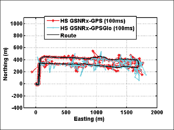
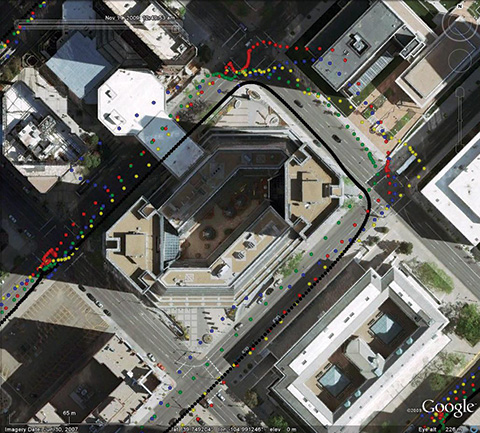
Finally, Figure 12 shows the trajectories obtained from the assisted HS receiver. In this case, the position solutions are significantly less noisy than in previous cases, in addition to being more available. The quality of the GPS-only and GPS+GLONASS results is broadly similar, with perhaps more outliers in the GPS-GLONASS case, due to the reason mentioned earlier.
Figure 12. Trajectories obtained using assisted HS GPS-GLONASS processing.
In summary, it would appear that the greatest benefit of GLONASS in this test was in the provision of greater redundancy in the navigation solution, in addition to potential better reliability, although the latter remains to be confirmed. With GLONASS approaching full operational capability, it is to be expected that the increased GLONASS constellation will lead to further improvements in terms of availability, DOP, and reliability.
Coherent Integration Time
From the preceding analysis it is clear that the assisted HS GNSS processing strategy yielded the best performance. To evaluate the impact of the coherent integration time on performance, the data was re-processed with a coherent integration time of 300 milliseconds (ms), instead of the 100 ms used for the data presented so far. The resulting trajectories are shown in Figure 13.
It is interesting to note that increasing the receiver sensitivity in this way does not yield better navigation performance. In fact, in the urban canyon environment, the major issue is not the signal attenuation (which can be overcome by increased coherent integration) but rather the multipath effect. By increasing the coherent integration time to 300 ms, the receiver becomes more sensitive to dynamics, resulting in poorer navigation performance.
Figure 13. Trajectories obtained using assisted HS GPS-GLONASS processing (300 ms integration time).
Discussion
High-sensitivity processing in urban canyon environments is a very effective means of improving navigation performance. Given the discussion above, however, it is clear that the performance is not limited by the strength of the received signal, but rather by the effect of multipath and satellite geometry.
The advantage of high-sensitivity processing in this case is two-fold. The first advantage over standard tracking techniques is the open-loop nature of HS processing. The time-varying nature of the multipath channel causes significant variation in signal level. This variation can cause traditional tracking loops to lose lock. In fact, the poor performance of the standard wide-correlator strategy in the above analysis can be explained by the fact that the receiver was unable to maintain lock on the satellites in view. Hence no measurements were generated, and no solutions computed. The survey-grade receiver used has advanced multipath mitigation technology, which helped to avoid loss of lock, but may have been tracking non-line-of-sight signals during portion of the down-town test, leading to errors in the navigation solution.
The second advantage of HS processing is related to the coherent integration time and the vehicle dynamics. As the receiver antenna moves through the multipath environment, a different Doppler shift is observed on signals coming from different directions. Thus the line-of-sight and multipath components become separated in frequency. A longer coherent integration time increases the frequency resolution of the correlator output (due to the familiar sinc shape). Thus if the line-of-sight is present, and the coherent integration time is long relative to the inverse of the Doppler difference between the line-of-sight and reflected signals, individual peaks become visible in the grid of correlators. This effect can significantly reduce the impact of multipath on the measurements. Figure 14 gives an example of this.
Figure 14. Sample correlation function showing two peaks.
Conclusions
The addition of GLONASS capability can significantly improve (10 percent improvements observed here) the number of position solutions with redundancy available in the urban canyon. With increasing GLONASS satellite availability, the benefits of using GLONASS will even be greater. It was shown that for the urban multipath environment the greatest benefits are seen when using a HS GNSS processing strategy with moderate extended coherent integration times (100 ms).
Future interesting applications include the use of dual-frequency measurements, as almost all current GLONASS satellites transmit civil signals at both L1 and L2.
Acknowledgments
The authors would like to kindly acknowledge and thank Defence Research and Development Canada (DRDC) for partly funding this work.
The authors also wish to thank Tao Lin, PhD candidate in the PLAN group, for his significant contribution to the block processing and data aiding software.
Manufacturers
The tests used a National Instruments PXI-5661 RF downconverter and digitizer, the PLAN GSNRx as standard wide-correlator receiver, the u-blox Antaris 4 (standalone HS-GPS), NovAtel OEMV-3 (survey-grade GPS/GLONASS), and the PLAN group software receiver GSNRx, as the assisted HS GPS/GLONASS.
Cillian O’Driscoll received his Ph.D. in 2007 from the Department of Electrical and Electronic Engineering, University College Cork, and is currently a post-doctoral fellow in the PLAN Group of the University of Calgary.
Gérard Lachapelle is a professor of geomatics engineering at the University of Calgary where he holds a Canada Research Chair in wireless location and heads the Position, Location and Navigation (PLAN) Group.
Mohamed Tamazin is a M.Sc. candidate in the the PLAN at the University of Calgary. He holds a M.Sc. in electrical communications from the Arab Academy for Science and Technology, Alexandria, Egypt.
The European GNSS Agency (GSA) has published a 2010 GNSS Market Monitoring report, providing key information in support of entrepreneurship in the satellite navigation sector.
GNSS market forecasting is of great interest to private and public GNSS stakeholders, for business and strategic planning and policymaking, said the GSA. According to the new report, the market for GNSS will grow significantly over the next decade, at a compound annual growth rate (CAGR) of 11 percent, reaching €165 billion for the core GNSS market in 2020. Delivery of GNSS devices will exceed one billion per year by 2020.
“This Report confirms that the market potential of GNSS is significant,” said Gian Gherardo Calini, head of the GSA Market Development Department. “The information should be useful to researchers, market players and decision makers who want to grasp the GNSS market opportunities today and tomorrow.”
Report Highlights
Road leads the way: The report shows that the road transport sector is still the leading GNSS segment, accounting for more than 50% of market share. The penetration of receivers in road vehicles, today at 30%, will exceed 80% over the next decade. However, after a period of fast growth, market saturation and competition in the form of ‘smartphones’, often equipped with free navigation capabilities, have resulted in a slowdown in the car-based navigation market.
Price erosion has been high, driven by declining costs and strong competition. Vendors are using innovation as a differentiator resulting in ‘converged’ products with both communication and multimedia functionalities. Some Personal Navigation Device (PND) vendors are also tapping into new distribution channels, including car dealerships and smartphone application stores.
GNSS for road transport: The road transport sector is facing major challenges, such as the demand for increasing safety and for reduced congestion and pollution. These problems are particularly acute in highly populated zones, including big cities and suburban areas. GNSS represents a powerful tool for improving road transport. Not only does it help get drivers where they want to go more quickly and efficiently, but it also promises fairer road-pricing schemes, for example, to automatically charge drivers for the use of road infrastructure.
GNSS in your hands. Mobile location-based services (LBS) are taking off as progress is being made in different areas. More and more mobile phones now have GNSS capabilities, the result of both increasing consumer and developer awareness and an improvement in navigation services and performance.
All major mobile phone operating system vendors now provide application programming interfaces (API) with location functions. In 2009, in the UK, France and Germany, 5 out of the 10 best-selling iPhone applications were related to navigation or location-based applications. Also, 30% of Android developers’ contest winners used location capabilities in their applications.
A promising future for location-based services. The integration of accurate hand-held positioning signal receivers, within mobile telephones, personal digital assistants (PDAs), mp3 players, portable computers, even digital cameras and video devices, brings GNSS services directly to individuals, making possible a fundamental transformation of the way we work and play. The penetration of GNSS in mobile phones is therefore expected to increase very quickly, from some 20% today to above 50% within the next five years.
The GSA says Galileo in the future and EGNOS today open up new and exciting prospects for economic growth, benefiting citizens, businesses and governments throughout the EU and beyond.
Just the beginning. The GSA underlines that the GNSS Market Monitoring process is ongoing and future reports are planned to update information presented in this first report and to cover other sectors. The Agency welcomes stakeholder contributions.
By Axel van den Berg, Tom Willems, Graham Pye, and Wim de Wilde, Septentrio Satellite Navigation, Richard Morgan-Owen, Juan de Mateo, Simone Scarafia, and Martin Hollreiser, European Space Agency
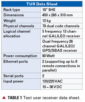
A fully stand-alone, multi-frequency, multi-constellation receiver unit, the TUR-N can autonomously generate measurements, determine its position, and compute the Galileo safety-of-life integrity.
Development of a reference Galileo Test User Receiver (TUR) for the verification of the Galileo in-orbit validation (IOV) constellation, and as a demonstrator for multi-constellation applications, has culminated in the availability of the first units for experimentation and testing. The TUR-N covers a wide range of receiver configurations to demonstrate the future Galileo-only and GPS/Galileo combined services:
Galileo single- and dual-frequency Open Services (OS)
Galileo single- and dual-frequency safety-of-life services (SoL), including the full Galileo navigation warning algorithms
Galileo Commercial Service (CS), including tracking and decoding of the encrypted E6BC signal
GPS/SBAS/Galileo single- and dual- frequency multi-constellation positioning
Galileo single- and dual-frequency differential positioning.
Galileo triple-frequency RTK.
In parallel, a similar test user receiver is specifically developed to cover the Public Regulated service (TUR-P). Without the PRS components and firmware installed, the TUR-N is completely unclassified.
Main Receiver Unit
The TUR-N receiver is a fully stand-alone, multi-frequency, multi-constellation receiver unit. It can autonomously generate measurements, determine its position, and compute Galileo safety-of-life integrity, which is output in real time and/or stored internally in a compact proprietary binary data format.
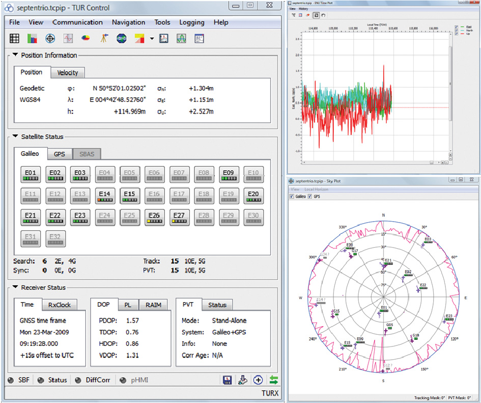
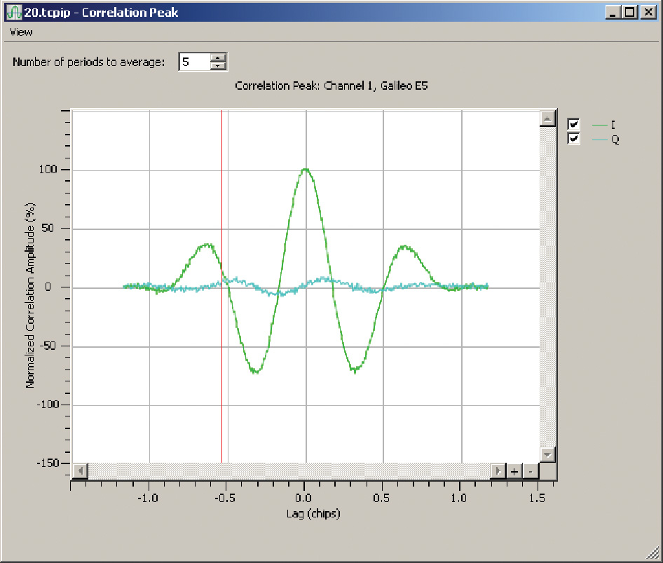
The receiver configuration is fully flexible via a command line interface or using the dedicated graphical user interface (GUI) for monitoring and control. With the MCA GUI it is also possible to monitor the receiver operation (see Figure 1), to present various real-time visualizations of tracking, PVT and integrity performances, and off-line analysis and reprocessing functionalities. Figure 2 gives an example of the correlation peak plot for an E5 AltBOC signal.
FIGURE 1. TUR-N control screen.FIGURE 2. E5 AltBOC correlation peak.
A predefined set of configurations that map onto the different configurations as prescribed by the Test User Segment Requirements (TUSREQ) document is provided by the receiver.
The unit can be included within a local network to provide remote access for control, monitoring, and/or logging, and supports up to eight parallel TCP/IP connections; or, a direct connection can be made via one of the serial ports.
Receiver Architecture
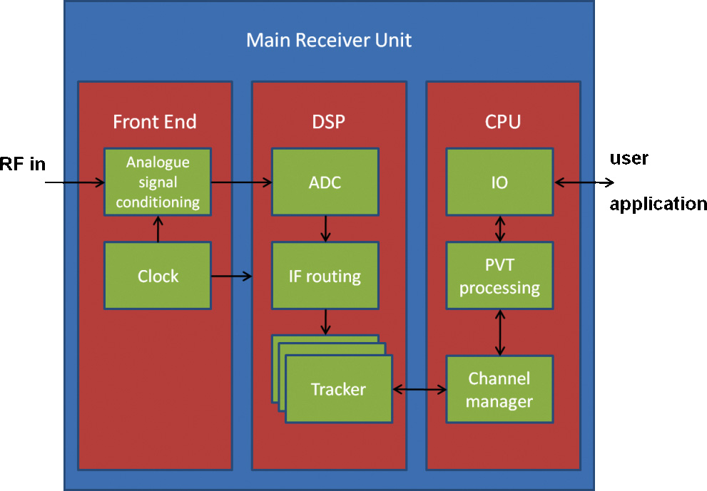
The main receiver unit consists of three separate boards housed in a standard compact PCI 19-inch rack. See Figure 3 for a high-level architectural overview.
FIGURE 3. Receiver architecture.
A dedicated analog front-end board has been developed to meet the stringent interference requirements. This board contains five RF chains for the L1, E6, E5a/L5, E5b, and E5 signals. Via a switch the E5 signal is either passed through separate filter paths for E5a and E5b or via one wide-band filter for the full E5 signal. The front-end board supports two internal frequency references (OCXO or TCXO) for digital signal processing (DSP).
The DSP board hosts three tracker boards derived from a commercial dual-frequency product family. These boards contain two tracking cores, each with a dedicated fast-acquisition unit (FAU), 13 generic dual-code channels, and a 13-channel hardware Viterbi decoder. One tracking core interacts with an AES unit to decrypt the E6 Commercial Service carrier; it has a throughput of 149 Mbps.
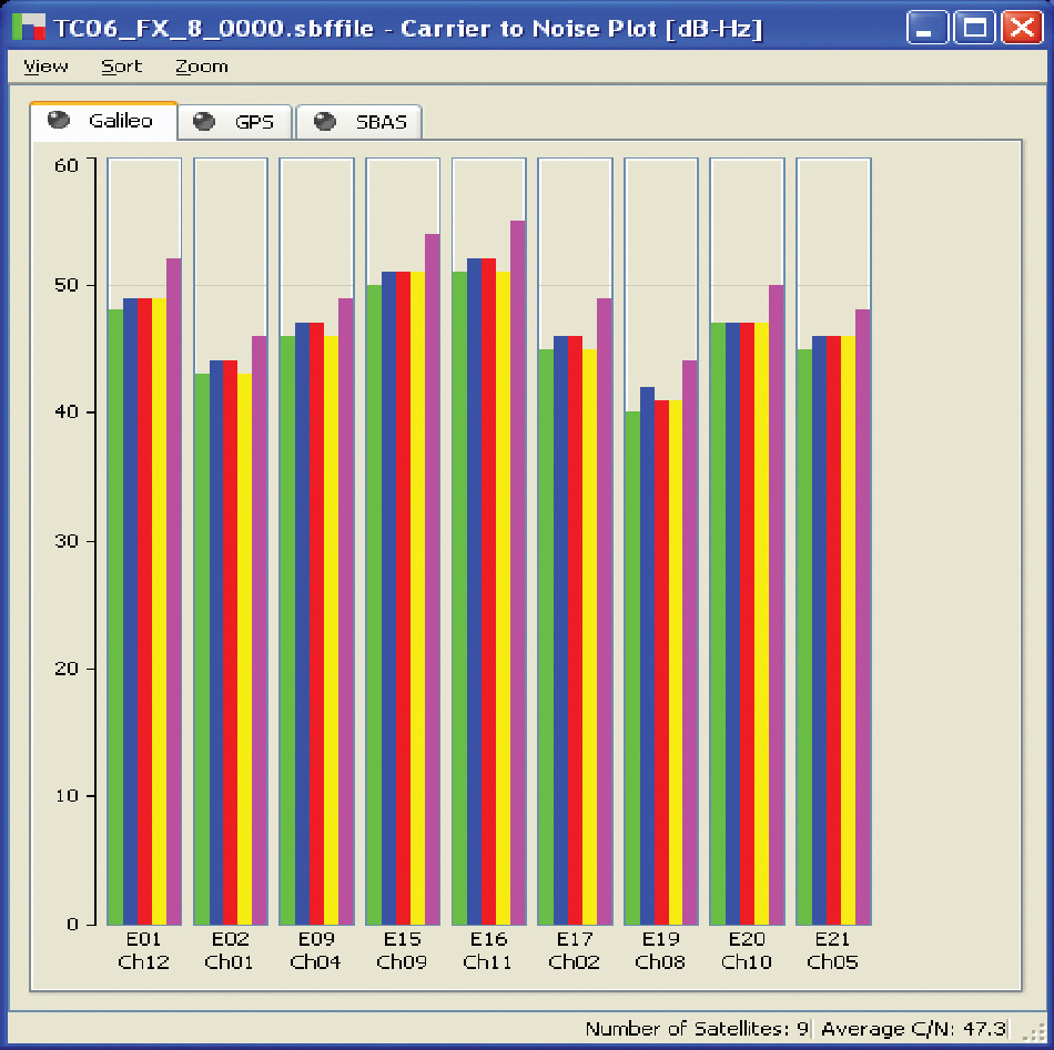
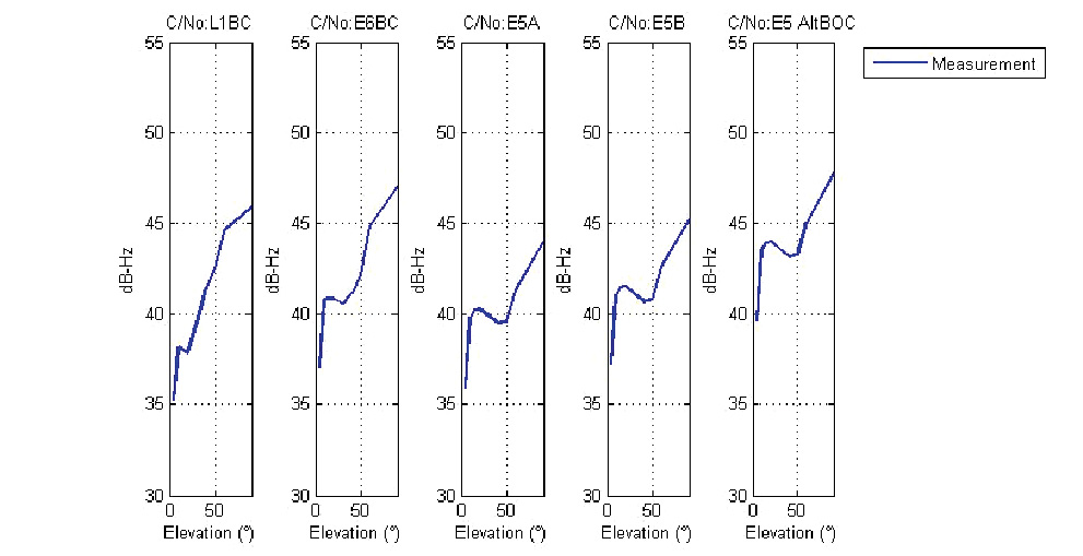
Each FAU combines a matched filter with a fast Fourier transform (FFT) and can verify up to 8 million code-frequency hypotheses per second. Each of the six tracker cores can be connected with one of the three or four incoming IF streams. To simplify operational use of the receiver, two channel-mapping files have been defined to configure the receiver either for a 5-frequency 13-channel Galileo receiver, or for a dual-frequency 26-channel Galileo/GPS/SBAS receiver. Figure 4 shows all five Galileo signal types being tracked for nine visible satellites at the same time.
FIGURE 4. C/N0 plot with nine satellites and all five Galileo signal types: L1BC (green), E6BC (blue), E5a (red), E5b (yellow), and E5 Altboc (purple).
The receiver is controlled using a COTS CPU board that also hosts the main positioning and integrity algorithms. The processing power and available memory of this CPU board is significantly higher than what is normally available in commercial receivers. Consequently there is no problem in supporting the large Nequick model used for single-frequency ionosphere correction, and achieving the 10-Hz update rate and low latency requirements when running the computationally intensive Galileo integrity algorithms. For commercial receivers that are normally optimized for size and power consumption, these might prove more challenging.
The TUR project included development of three types of Galileo antennas:
a triple-band (L1, E6, E5) high-end antenna for fixed base station applications including a choke ring;
a triple-band (L1, E6, E5) reference antenna for rover applications;
a dual-band (L1, E5b) aeronautic antenna for SOL applications
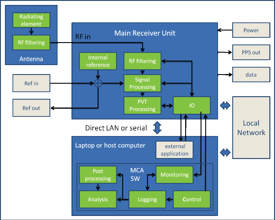
Figure 5 shows an overview of the main interfaces and functional blocks of the receiver, together with its antenna and a host computer to run the MCA software either remotely or locally connected.
FIGURE 5. TUR-N with antenna and host computer.
Receiver Verification
Currently, the TUR-N is undergoing an extensive testing program. In order to fully qualify the receiver to act as a reference for the validation of the Galileo system, some challenges have to be overcome. The first challenge that is encountered is that the performance verification baseline is mainly defined in terms of global system performance. The translation of these global requirements derived from the Galileo system requirements (such as global availability, accuracy, integrity and continuity, time-to-first/precise-fix) into testable parameters for a receiver (for example, signal acquisition time, C/N0 versus elevation, and so on) is not trivial. System performances must be fulfilled in the worst user location (WUL), defined in terms of dynamics, interference, and multipath environment geometry, and SV-user geometry over the Galileo global service area.
A second challenge is the fact that in the absence of an operational Galileo constellation, all validation tests need to be done in a completely simulated environment. First, it is difficult to assess exactly the level of reality that is necessary for the various models of the navigation data quality, the satellite behaviour, the atmospheric propagation effects, and the local environmental effects. But the main challenge is that not only the receiver that is being verified, also the simulator and its configuration are an integral part of the verification. It is thus an early experience of two independent implementations of the Galileo signal-in-space ICD being tested together. At the beginning of the campaign, there was no previously demonstrated or accepted test reference.
Only the combined efforts of the various receiver developments benchmarked against the same simulators together with pre-launch compatibility tests with the actual satellite payload and finally IOV and FOC field test campaigns will ultimately validate the complete system, including the Galileo ground and space segments together with a limited set of predefined user segment configurations. (Previously some confidence was gained with GIOVE-A/B experimental satellites and a breadboard adapted version of TUR-N). The TUR-N was the first IOV-compatible receiver to be tested successfully for RF compatibility with the Galileo engineering model satellite payload.
Key Performances
Receiver requirements, including performance, are defined in the TUSREQ document.
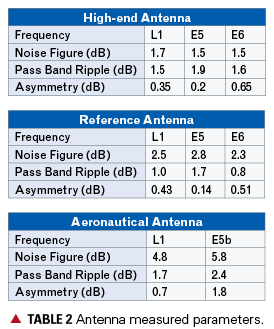
Antenna and Interference. A key TUSREQ requirement focuses on receiver robustness against interference. It has proven quite a challenge to meet the prescribed interference mask for all user configurations and antenna types while keeping many other design parameters such as gain, noise figure, and physical size in balance. For properly testing against the out-of-band interference requirements, it also proved necessary to carefully filter out increased noise levels created by the interference signal generator.
Table 2 gives an overview of the measured values for the most relevant Antenna Front End (AFE) parameters for the three antenna types. Note: Asymmetry in the AFE is defined as the variation of the gain around the centre frequency in the passband. This specification is necessary to preserve the correlation peak shape, mainly of the PRS signals.
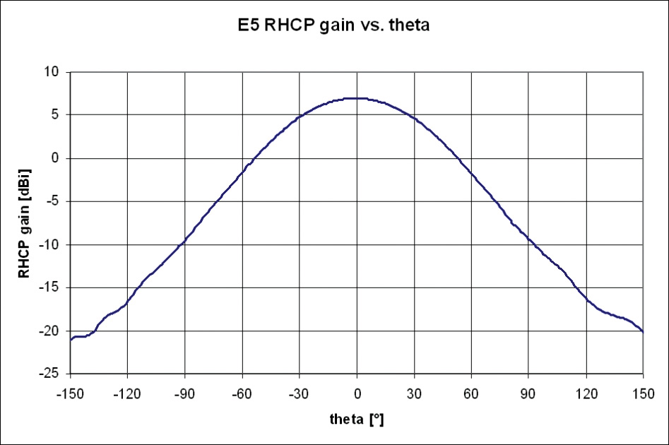
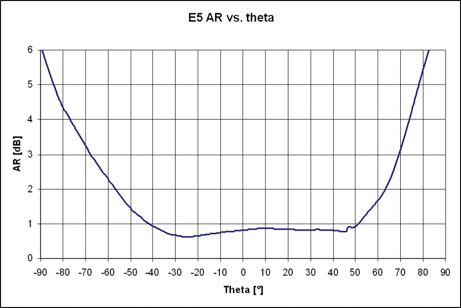
The gain for all antenna front ends and frequencies is around 32 dB. Figures 6 and 7 give an example of the measured E5 RHCP radiating element gain and axial ratio against theta (the angle of incidence with respect to zenith) for the high-end antenna-radiating element. Thus, elevation from horizontal is 90-theta.
UERE Performance. As part of the test campaign, TUR performance has been measured for user equivalent range error (UERE) components due to thermal noise and multipath.
TUSREQ specifies the error budget as a function of elevation, defined in tables at the following elevations: 5, 10, 15, 20, 30, 40, 50, 60, 90 degrees. The elevation dependence of tracking noise is immediately linked to the antenna gain pattern; the antenna-radiating element gain profiles were measured on the actual hardware and loaded to the Radio Frequency Constellation Simulator (RFCS), one file per frequency and per antenna scenario. The RFCS signal was passed through the real antenna RF front end to the TUR. As a result, through the configuration of RFCS, real environmental conditions (in terms of C/N0) were emulated in factory.
The thermal noise component of the UERE budget was measured without multipath being applied, and interference was allowed for by reducing the C/N0 by 3 dB from nominal. Separately, the multipath noise contribution was determined based on TUSREQ environments, using RFCS to simulate the multipath (the multipath model configuration was adapted to RFCS simulator multipath modeling capabilities in compliance with TUSREQ). To account for the fact that multipath is mostly experienced on the lower elevation satellites, results are provided with scaling factors applied for elevation (“weighted”), and without scaling factors (“unweighted”). In addition, following TUSREQ requirements, a carrier smoothing filter was applied with 10 seconds convergence time.
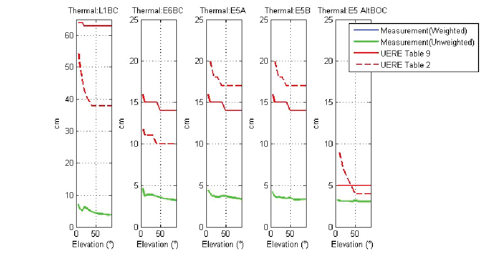
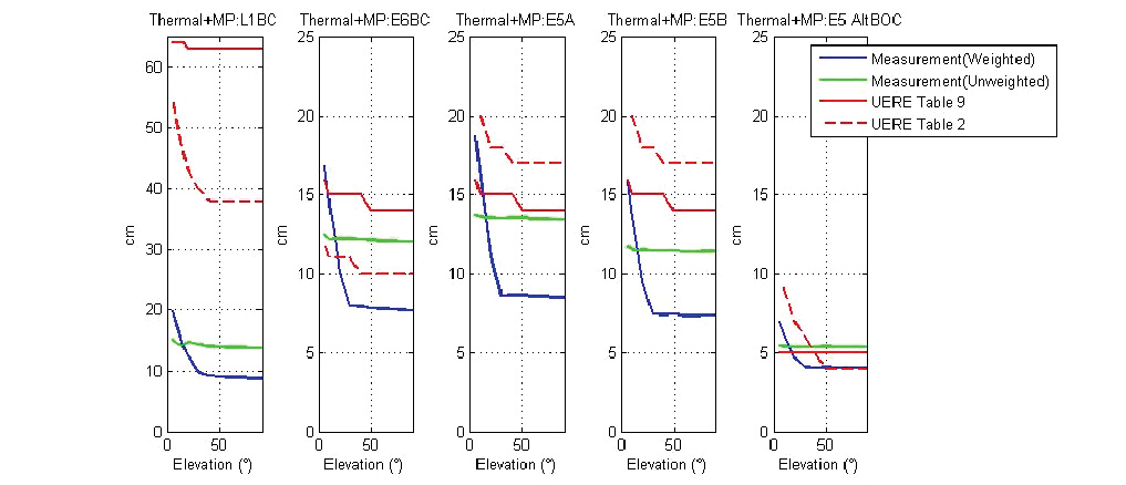
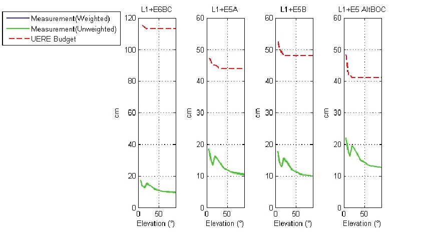
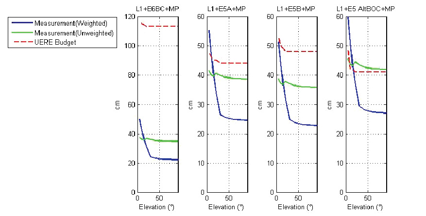
Figure 8 shows the C/N0 profile from the reference antenna with nominal power reduced by 3 dB. Figure 9 shows single-carrier thermal noise performance without multipath, whereas Figure 10 shows thermal noise with multipath. Each of these figures includes performance for five different carriers: L1BC, E6BC, E5a, E5b, and E5 AltBOC, and the whole set is repeated for dual-frequency combinations (Figure 11 and Figure 12).
FIGURE 8. Reference antenna, power nominal-3 dB, C/N0 profile.FIGURE 9. Reference antenna, power nominal-3 dB, thermal noise only, single frequency.FIGURE 10. Reference antenna, power nominal-3 dB, thermal noise with multipath, single frequency.FIGURE 11. Reference antenna, power nominal-3 dB, thermal noise only, dual frequency.FIGURE 12. Reference antenna, power nominal-3 dB, thermal noise with multipath, dual frequency.
The plots show that the thermal noise component requirements are easily met, whereas there is some limited non-compliance on noise+multipath (with weighted multipath) at low elevations. The tracking noise UERE requirements on E6BC are lower than for E5a, due to assumption of larger bandwidth at E6BC (40MHz versus 20MHz). Figures 9 and 10 refer to UERE tables 2 and 9 of TUSREQ. The relevant UERE requirement for this article is TUSREQ table 2 (satellite-only configuration). TUSREQ table 9 is for a differential configuration that is not relevant here.
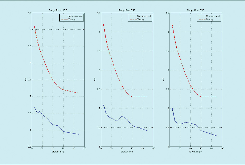
UERRE Performance. The complete single-frequency range-rate error budget as specified in TUSREQ was measured with the RFCS, using a model of the reference antenna. The result in Figure 13 shows compliance.
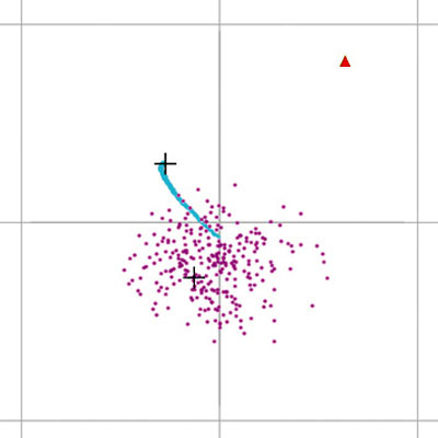
FIGURE 13. UERRE measurements.FIGURE 14. L1 GPS CA versus E5 AltBOC position accuracy (early test result).
Position Accuracy. One of the objectives of the TUR-N is to demonstrate position accuracy. In Figure 14 an example horizontal scatter plot of a few minutes of data shows a clear distinction between the performances of two different single-frequency PVT solutions: GPS L1CA in purple and E5AltBOC in blue. The red marker is the true position, and the grid lines are separated at 0.5 meters. The picture clearly shows how the new E5AltBOC signal produces a much smoother position solution than the well-known GPS L1CA code. However, these early results are from constellation simulator tests without the full TUSREQ worst-case conditions applied.
FIGURE 14. L1 GPS CA versus E5 AltBOC position accuracy (early test result).
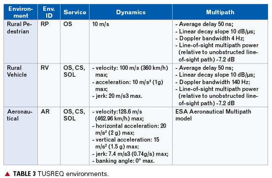
The defined TUSREQ user environments, the basis for all relevant simulations and tests, are detailed in Table 3. In particular, the rural pedestrian multipath environment appears to be very stringent and a performance driver.
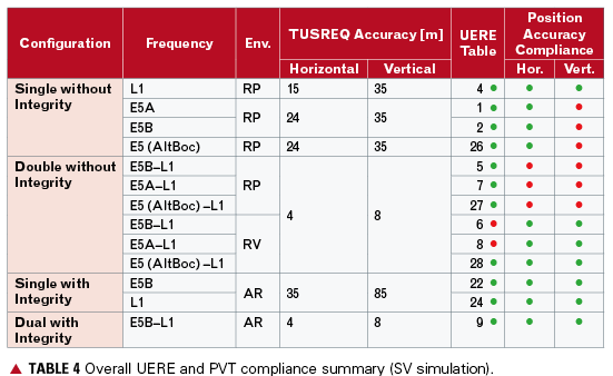
This was already identified at an early stage during simulations of the total expected UERE and position accuracy performance compliance with regard to TUSREQ, summarized in Table 4, and is now confirmed with the initial verification tests in Figure 10. UERE (simulated) total includes all other expected errors (ionosphere, troposphere, ODTS/BGD error, and so on) in addition to the thermal noise and multipath, whereas the previous UERE plots were only for selected UERE components. The PVT performance in the table is based on service volume (SV) simulations.
The non-compliances on position accuracy that were predicted by simulations are mainly in the rural pedestrian environment. According to the early simulations:
E5a and E5b were expected to have 43-meter vertical accuracy (instead of 35-meter required).
L1/E5a and L1/E5b dual-frequency configurations were expected to have 5-meter horizontal, 12-meter vertical accuracy (4 and 8 required).
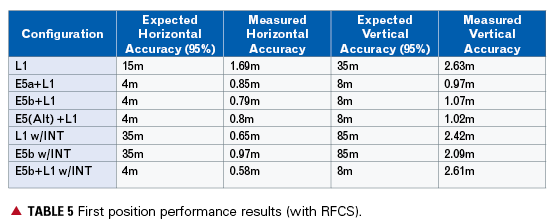
These predictions appear pessimistic related to the first position accuracy results shown in Table 5. On single frequency, the error is dominated by ionospheric delay uncertainty. These results are based on measurements using the RFCS and modeling the user environment; however, the simulation of a real receiver cannot be directly compared to service-volume simulation results, as a good balance between realism and worst-case conditions needs to be found. Further optimization is needed on the RFCS scenarios and on position accuracy pass/fail criteria to account for DOP variations and the inability to simulate worst environmental conditions continuously.
Further confirmations on Galileo UERE and position accuracy performances are expected after the site verifications (with RFCS) are completed, and following IOV and FOC field-test campaigns.
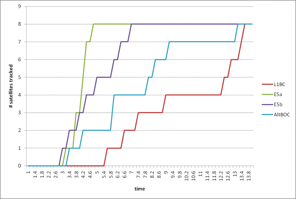
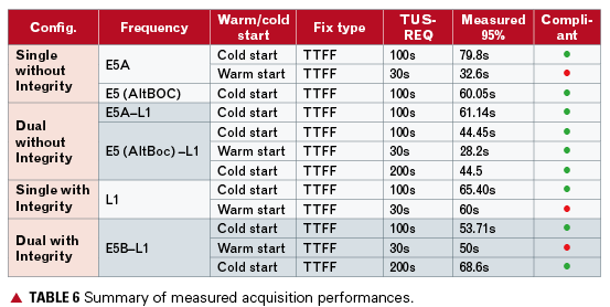
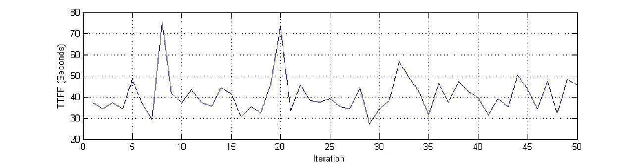
Acquisition. Figure 15 gives an example of different signal-acquisition times that can be achieved with the TUR-N after the receiver boot process has been completed. Normally, E5 frequencies lock within 3 seconds, and four satellites are locked within 10 seconds for all frequencies. This is based on an unaided (or free) search using a FAU in single-frequency configurations, in initial development test without full TUSREQ constraints.
FIGURE 15. Unaided acquisition performance.
When a signal is only temporarily lost due to masking, and the acquisition process is still aided (as opposed to free search), the re-acquisition time is about 1 second, depending on the signal strength and dynamics of the receiver. When the PVT solution is lost, the aiding process will time out and return to free search to be robust also for sudden user dynamics.
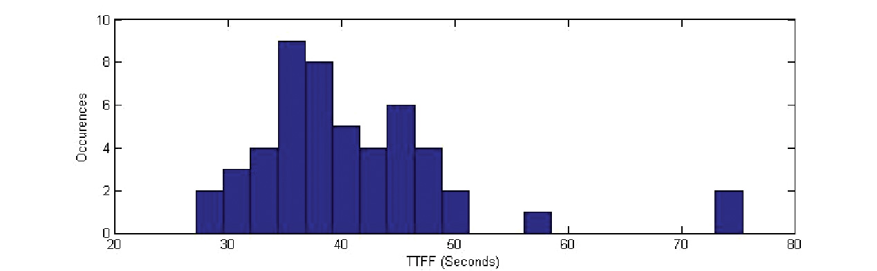
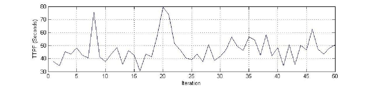
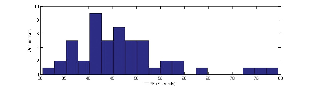
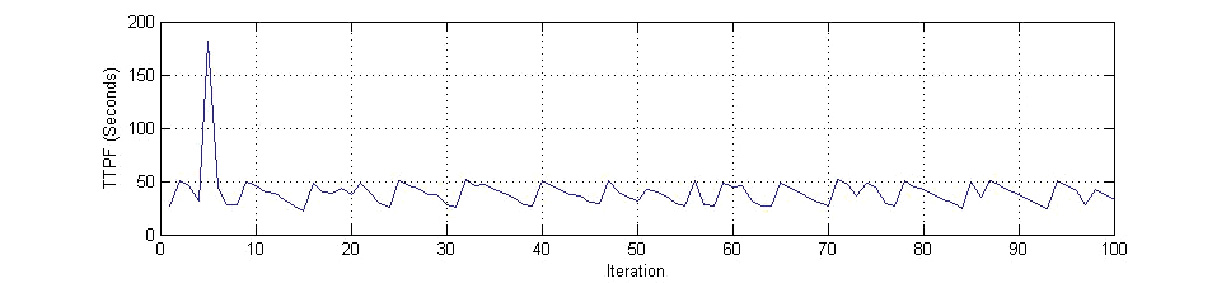
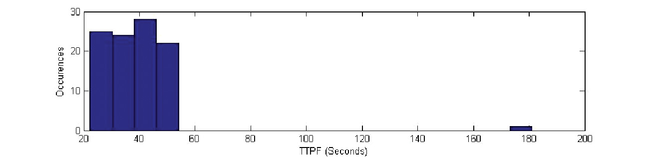
More complete and detailed time-to-first-fix (TTFF) and time-to-precise-fix (TTPF), following TUSREQ definitions, have also been measured.
In cold start the receiver has no prior knowledge of its position or the navigation data, whereas in warm start it already has a valid ephemeris in memory (more details on start conditions are available in TUSREQ). Table 6 shows that the acquisition performances measured are all compliant to TUSREQ except for warm start in E5a single frequency and in the integrity configurations. However, when the navigation/integrity message recovery time is taken off the measurement (as now agreed for updated TUSREQ due to message limitations), these performances also become compliant.
Specific examples of statistics gathered are shown in figures 16–21, these examples being for dual-frequency (E5b+L1) with integrity configuration. The outliers, being infrequent results with high acquisition times, are still compliant with the maximum TTFF/TTPF requirements, but are anyway under further investigation.
FIGURE 16. TTFF cold-start performance, dual frequency with integrity E5b+L1.FIGURE 17. TTFF cold-start distribution, dual frequency with integrity E5b+L1.FIGURE 18. TTPF cold-start performance, dual frequency with integrity E5b+L1.FIGURE 19. TTPF cold-start distribution, dual frequency with integrity E5b+L1.FIGURE 20. TTFF warm-start performance, dual frequency with integrity E5b+L1.FIGURE 21. TTFF warm-start distribution, dual frequency with integrity E5b+L1,
Integrity Algorithms. The Galileo SoL service is based on a fairly complex processing algorithm that determines not only the probability of hazardous misleading information (PHMI) based on the current set of satellites used in the PVT computation (HPCA), but also takes into consideration the PHMI that is achieved when one of the satellites used in the current epoch of the PVT computation is unexpectedly lost within the following 15 seconds. PHMI is computed according to alarm limits that are configurable for different application/service levels. These integrity algorithms have been closely integrated into the PVT processing routines, due to commonality between most processing steps.
Current test results of the navigation warning algorithm (NWA) indicate that less than 10 milliseconds of processing time is required for a full cycle of the integrity algorithms (HPCA+CSPA) on the TUR-N internal CPU board. Latency of the availability of the integrity alert information in the output of the receiver after it was transmitted by the satellite has been determined to be below 400 milliseconds. At a worst-case data output rate of 10 Hz this can only be measured in multiples of 100 millisecond periods. The total includes 100 milliseconds of travel time of the signal in space and an estimated 250 milliseconds of internal latency for data-handling steps as demodulation, authentication, and internal communication to make the data available to the integrity processing.
Conclusions
The TUR-N is a fully flexible receiver that can verify many aspects of the Galileo system, or as a demonstrator for Galileo/GPS/SBAS combined operation. It has a similar user interface to commercial receivers and the flexibility to accommodate Galileo system requirements evolutions as foreseen in the FOC phase without major design changes.
The receiver performance is in general compliant with the requirements. For the important safety-of-life configuration, major performance requirements are satisfied in terms of acquisition time and position accuracy.
The receiver prototype is currently operational and undergoing its final verification and qualification, following early confirmations of compatibility with the RFCS and with the Galileo satellite payload.
Enhancing GNSS Receiver Sensitivity by Combining Signals from Multiple Satellites
By Penina Axelrad, James Donna, Megan Mitchell, and Shan Mohiuddin
A new approach to enhancing signal sensitivity combines the received signal power from multiple satellites in a direct-to-navigation solution.
INNOVATION INSIGHTS by Richard Langley
ALTHOUGH I HAVE MANAGED the Innovation column continuously since GPS World’s first issue, it wasn’t until the second issue that I authored a column article. That article, co-written with Alfred Kleusberg, was titled “The Limitations of GPS.” It discussed some of the then-current problems of GPS, including poor signal reception, loss of signal integrity, and limited positioning accuracy.
In the ensuing 20 years, both signal integrity and positioning accuracy have improved significantly. Advances in the GPS control segment’s capabilities to continuously monitor and assess signal performance, together with receiver-autonomous integrity monitoring and integrity enhancement provided by augmentation systems, have reduced worries about loss of signal integrity. The removal of Selective Availability and use of error corrections provided by augmentation systems, among other approaches, have improved positioning accuracy.
But the problem of poor reception due to weak signals is still with us. In that March/April 1990 article, we wrote “[GPS] signals propagate from the satellites to the receiver antenna along the line of sight and cannot penetrate water, soil, walls, or other obstacles very well. … In surface navigation and positioning applications, the signal can be obstructed by trees, buildings, and bridges. … [In] the inner city streets of urban areas lined with skyscrapers, the ‘visibility’ of the GPS satellites is very limited. In such areas, the signals can be obstructed for extended periods of time or even [be] continuously unavailable.”
Poor signal reception in other than open-sky environments is still a problem with conventional GPS receivers. However, extending signal integration times and using assisted-GPS techniques can give GPS some degree of capability to operate indoors and in other restricted environments, albeit typically with reduced positioning accuracy. An antenna with sufficient gain is needed and capable systems are available on the market. The pilot channels of modernized GNSS signals will also benefit signal acquisition and tracking in challenging environments.
In this month’s column, we look at a completely different approach to enhancing signal sensitivity. Rather than requiring each satellite’s signal to be acquired and tracked before it can be used in the navigation solution, the new approach — dubbed “collective detection” — combines the received signal power from multiple satellites in a direct-to-navigation-solution procedure. Besides providing a quick coarse position solution with weak signals, this approach can be used to monitor the signal environment, aid deeply-coupled GPS/inertial navigation, and assist with terrain and feature recognition.
“Innovation” features discussions about advances in GPS technology, its applications, and the fundamentals of GPS positioning. The column is coordinated by Richard Langley, Department of Geodesy and Geomatics Engineering, University of New Brunswick.
Growing interest in navigating indoors and in challenging urban environments is motivating research on techniques for weak GPS signal acquisition and tracking. The standard approach to increasing acquisition and tracking sensitivity is to lengthen the coherent integration times, which can be accomplished by using the pilot channels in the modernized GPS signals or by using assisted GPS (A-GPS) techniques. These techniques operate in the traditional framework of independent signal detection, which requires a weak signal to be acquired and tracked before it is useful for navigation. This article explores a complementary, but fundamentally different, approach that enhances signal sensitivity by combining the received power from multiple GPS satellites in a direct-to-navigation-solution algorithm. As will be discussed in the following sections, this collective detection approach has the advantage of incorporating into the navigation solution information from signals that are too weak to be acquired and tracked, and it does so with a modest amount of computation and with no required hardware changes. This technology is appropriate for any application that requires a navigation solution in a signal environment that challenges traditional acquisition techniques. Collective detection could be used to monitor the signal environment, aid deeply coupled GPS/INS during long outages, and help initiate landmark recognition in an urban environment. These examples are explained further in a subsequent section. In order to understand how the collective detection algorithm works, it is instructive to first consider the traditional approach to acquisition and tracking.
Acquisition Theory and Methods
In a typical stand-alone receiver, the acquisition algorithm assesses the signal’s correlation power in discrete bins on a grid of code delay and Doppler frequency (shift). The correlation calculations take the sampled signal from the receiver’s RF front end, mix it with a family of receiver-generated replica signals that span the grid, and sum that product to produce in-phase (I) and quadrature (Q) correlation output. The correlation power is the sum of the I and Q components, I2 + Q2. Plotting the power as a function of delay and frequency shift produces a correlogram, as shown in FIGURE 1. It should be noted that both correlation power and its square root, the correlation amplitude, are found in the GPS literature. For clarity, we will always use the correlation power to describe signal and noise values.
If a sufficiently powerful signal is present, a distinct peak appears in the correlogram bin that corresponds to the GPS signal’s code delay and Doppler frequency. If the peak power exceeds a predefined threshold based on the integration times and the expected carrier-to-noise spectral density, the signal is detected. The code delay and Doppler frequency for the peak are then passed to the tracking loops, which produce more precise measurements of delay — pseudoranges — from which the receiver’s navigation solution is calculated. When the satellite signal is attenuated, however, perhaps due to foliage or building materials, the correlation peak cannot be distinguished and the conventional approach to acquisition fails.
The sensitivity of traditional tracking algorithms is similarly limited by the restrictive practice of treating each signal independently. More advanced tracking algorithms, such as vector delay lock loops or deeply integrated filters, couple the receiver’s tracking algorithms and its navigation solution in order to take advantage of the measurement redundancy and to leverage information gained from tracking strong signals to track weak signals. The combined satellite detection approach presented in this article extends the concept of coupling to acquisition by combining the detection and navigation algorithms into one step.
Collective Detection
In the collective detection algorithm, a receiver position and clock offset grid is mapped to the individual GPS signal correlations, and the combined correlation power is evaluated on that grid instead of on the conventional independent code delay and Doppler frequency grids. The assessment of the correlation power on the position and clock offset grid leads directly to the navigation solution. The mapping, which is key to the approach, requires the receiver to have reasonably good a priori knowledge of its position, velocity, and clock offset; the GPS ephemerides; and, if necessary, a simplified ionosphere model. Given this knowledge, the algorithm defines the position and clock offset search grid centered on the assumed receiver state and generates predicted ranges and Doppler frequencies for each GPS signal, as illustrated in FIGURE 2. The mapping then relates each one of the position and clock offset grid points to a specific code delay and Doppler frequency for each GPS satellite, as illustrated in FIGURE 3. Aggregating the multiple delay/Doppler search spaces onto a single position/clock offset search space through the mapping allows the navigation algorithm to consider the total correlation power of all the signals simultaneously. The correlation power is summed over all the GPS satellites at each position/clock-offset grid point to create a position domain correlogram. The best position and clock-offset estimates are taken as the grid point that has the highest combined correlation power. This approach has the advantage of incorporating into the position/clock-offset estimate information contained in weak signals that may be undetectable individually using traditional acquisition/tracking techniques.
It should be noted that a reasonable a priori receiver state estimate restricts the size of the position and clock-offset grid such that a linear mapping, based on the standard measurement sensitivity matrix used in GPS positioning, from the individual signal correlations, is reasonable. Also, rather than attempt to align the satellite correlations precisely enough to perform coherent sums, noncoherent sums of the individual satellite correlations are used. This seems reasonable, given the uncertainties in ranging biases between satellites, differences and variability of the signal paths through the ionosphere and neutral atmosphere, and the large number of phases that would have to be aligned.
Applications
The most obvious application for collective detection is enabling a navigation fix in circumstances where degraded signals cause traditional acquisition to fail. The sweet spot of collective detection is providing a rapid but coarse position solution in a weak signal environment. The solution can be found in less time because information is evaluated cohesively across satellites. This is especially clear when the algorithm is compared to computationally intensive long integration techniques.
There are several ways that collective detection can support urban navigation. This capability benefits long endurance users who desire a moderate accuracy periodic fix for monitoring purposes. In some circumstances, the user may wish to initiate traditional tracking loops for a refined position estimate. However, if the signal environment is unfavorable at the time, this operation will waste valuable power. The collective detection response indicates the nature of the current signal environment, such as indoors or outdoors, and can inform the decision of whether to spend the power to transition to full GPS capabilities.
In urban applications, deeply integrated GPS/INS solutions tolerate GPS outages by design. However, if the outage duration is too long, the estimate uncertainty will eventually become too large to allow conclusive signal detection to be restored. Running collective detection as a background process could keep deeply integrated filters centered even in long periods of signal degradation. Because collective detection approaches the acquisition problem from a position space instead of the individual satellite line-of-sight space, it provides inherent integrity protection. In the traditional approach, acquiring a multipath signal will pollute the overall position fix. In collective detection, such signals are naturally exposed as inconsistent with the position estimate.
Another use would be to initialize landmark correlation algorithms in vision navigation. Landmark correlation associates street-level video with 3D urban models as an alternative to (GPS) absolute position and orientation updates. This technique associates landmarks observed from ground-level imagery with a database of landmarks extracted from overhead-derived 3D urban models. Having a coarse position (about 100 meters accuracy) enhances initialization and restart of the landmark correlation process. Draper Laboratory is planning to demonstrate the utility of using collective detection to enable and enhance landmark correlation techniques for urban navigation.
In all of these applications, collective detection is straightforward to implement because it simply uses the output of correlation functions already performed on GPS receivers.
Simulations and Processing
The new algorithm has been tested using live-sky and simulated data collected by a Draper Laboratory wideband data recorder. A hardware GPS signal simulator was used to simulate a stationary observer receiving 11 equally powered GPS signals that were broadcast from the satellite geometry shown in FIGURE 4. The data recorder and the signal simulator were set up in a locked-clock configuration with all of the simulator’s modeled errors set to zero. No frequency offsets should exist between the satellites and the receiver. A clock bias, however, does exist because of cable and other fixed delays between the two units. The data recorder houses a four-channel, 14-bit A/D module. It can support sample rates up to 100 MHz. For this work, it was configured to downconvert the signal to an IF of 420 kHz and to produce in-phase and quadrature samples at 10 MHz.
Results and Discussion
To combine satellites, a position domain search space is established, centered on the correct location and receiver clock bias. A grid spacing of 30 meters over a range of ± 900 meters in north and east directions, and ± 300 meters in the vertical. In the first simulated example, the correlation power for all the satellites is summed on the position grid using a single 1-millisecond integration period. In this case, the true carrier-to-noise-density ratio for each signal is 40 dB-Hz. The results are shown in FIGURE 5. The plots in the left panel show the individual signal correlations as a function of range error. The four plots in the upper-right panel show several views of the combined correlation as a function of position error. The upper-left plot in the panel shows the correlation value as a function of the magnitude of the position error. The upper-right plot shows the correlation as a function of the north-east error, the lower-left the north-down error, and the lower-right the east-down error. Notice how the shape of the constant power contours resembles the shape of the constant probability contours that would result from a least-squares solution’s covariance matrix. The final plot, the bottom-right panel, shows a 3D image of the correlation power as a function of the north-east error. It is clear in these images that in the 40 dB-Hz case each satellite individually reaches the highest correlation power in the correct bin and that the combined result also peaks in the correct bin. In the combined satellite results, each individual satellite’s correlation power enters the correlogram as the ridge that runs in a direction perpendicular to the receiver-satellite line-of-sight vector and represents a line of constant pseudorange.
FIGURE 6 shows a similar set of graphs for a simulator run at 20 dB-Hz. The plots in the left panel and the four plots in the upper-right panel show the individual and combined correlations, as in Figure 5. In the lower-right panel, the 3D image has been replaced with correlations calculated using 20 noncoherent 1-millisecond accumulations. The indistinct peaks in many of the individual correlations (left panel) suggest that these signals may not be acquired and tracked using traditional methods. Those signals, therefore, would not contribute to the navigation solution. Yet in the combined case, those indistinct peaks tend to add up and contribute to the navigation solution. These results indicate the feasibility of using the information in weak signals that may not be detectable using traditional methods and short acquisition times. The situation is further improved by increasing the number of noncoherent integration periods.
Impact of Reduced Geometry. Of course, it is a bit unrealistic to have 11 satellites available, particularly in restricted environments, so we also considered three subsets of four-satellite acquisitions, under the same signal levels. FIGURE 7 compares the position domain correlograms for the following 20 dB-Hz cases: (1) a good geometry case (PRNs 3, 14, 18, 26), (2) an urban canyon case where only the highest 4 satellites are visible (PRNs 15, 18, 21, 22), and (3) a weak geometry case where just a narrow wedge of visibility is available (PRNs 18, 21, 26, 29). As expected, the correlation power peak becomes less distinct as the satellite geometry deteriorates. The pattern of degradation, morphing from a distinct peak to a ridge, reveals that the position solution remains well constrained in some directions, but becomes poorly constrained in others. Again, this result is expected and is consistent with the behavior of conventional positioning techniques under similar conditions.
Focusing on Clock Errors. In some real-world situations, for example, a situation where a receiver is operating in an urban environment, it is possible for the position to be fairly well known, but the clock offset and frequency to have substantial uncertainty. FIGURE 8 shows how the combined satellites approach can be used to improve sensitivity when viewed from the clock bias and frequency domain. The figure presents example 1-millisecond correlograms of clock bias and clock drift for three 20 dB-Hz cases: (1) a single GPS satellite case; (2) a four-satellite, good geometry case; and (3) an 11-satellite, good geometry case. The assumed position solution has been offset by a random amount (generated with a 1-sigma of 100 meters in the north and east components, and 20 meters in the up component), but no individual satellite errors are introduced. These plots clearly show the improved capability for acquisition of the clock errors through the combining process.
Live Satellite Signals. FIGURE 9 shows combined correlograms derived from real data recorded using an outdoor antenna. The first example includes high-signal-level satellites with 1.5-second noncoherent integration. The second example includes extremely attenuated satellite signals with a long noncoherent integration period of six seconds.
The plots in the upper-left and upper-right panels show combined correlograms as a function of the north-east position error for satellite signals with carrier-to-noise-density ratios of 48 dB-Hz or higher. The plots in the lower-left and lower-right panels show combined correlograms resulting from much weaker satellites with carrier-to-noise-density ratios of roughly 15 to 19 dB-Hz, using a coherent integration interval of 20 milliseconds and a noncoherent interval of six seconds. FIGURE 10 shows one of the individual single-satellite correlograms. In this attenuated case, the individual satellite power levels are just barely high enough to make them individually detectable. This is the situation in which collective detection is most valuable.
Conclusions
The example results from a hardware signal simulator and live satellites show how the noncoherent combination of multiple satellite signals improves the GPS position error in cases where some of the signals are too weak to be acquired and tracked by traditional methods. This capability is particularly useful to a user who benefits from a rapid, but coarse, position solution in a weak signal environment. It may be used to monitor the quality of the signal environment, to aid deeply coupled navigation, and to initiate landmark recognition techniques in urban canyons. The approach does require that the user have some a priori information, such as a reasonable estimate of the receiver’s location and fairly accurate knowledge of the GPS ephemerides. Degradation in performance should be expected if the errors in these models are large enough to produce pseudorange prediction errors that are a significant fraction of a C/A-code chip. Absent that issue, the combined acquisition does not add significant complexity compared to the traditional approach to data processing. It can be used to enhance performance of existing acquisition techniques either by improving sensitivity for the current noncoherent integration times or by reducing the required integration time for a given sensitivity. Further development and testing is planned using multiple signals and frequencies.
Acknowledgments
The authors appreciate the contributions of David German and Avram Tewtewsky at Draper Laboratory in collecting and validating the simulator data; Samantha Krenning at the University of Colorado for assistance with the simulator data analysis and plotting; and Dennis Akos at the University of Colorado for many helpful conversations and for providing the Matlab software-defined radio code that was used for setting up the acquisition routines. This article is based on the paper “Enhancing GNSS Acquisition by Combining Signals from Multiple Channels and Satellites” presented at ION GNSS 2009, the 22nd International Technical Meeting of the Satellite Division of The Institute of Navigation, held in Savannah, Georgia, September 22–25, 2009.
The work reported in the article was funded by the Charles Stark Draper Laboratory Internal Research and Development program.
Manufacturers
Data for the analyses was obtained using a Spirent Federal Systems GSS7700 GPS signal simulator and a GE Fanuc Intelligent Platforms ICS-554 A/D module.
PENINA AXELRAD is a professor of aerospace engineering sciences at the University of Colorado at Boulder. She has been involved in GPS-related research since 1986 and is a fellow of The Institute of Navigation and the American Institute of Aeronautics and Astronautics.
JAMES DONNA is a distinguished member of the technical staff at the Charles Stark Draper Laboratory in Cambridge, Massachusetts, where he has worked since 1980. His interests include GNSS navigation in weak signal environments and integrated inertial-GNSS navigation.
MEGAN MITCHELL is a senior member of the technical staff at the Charles Stark Draper Laboratory. She is involved with receiver customization for reentry applications and GPS threat detection.
SHAN MOHIUDDIN is a senior member of the technical staff at the Charles Stark Draper Laboratory. His interests include GNSS technology, estimation theory, and navigation algorithms.
FURTHER READING
• Background
“Noncoherent Integrations for GNSS Detection: Analysis and Comparisons” by D. Borio and D. Akos in IEEE Transactions on Aerospace and Electronic Systems, Vol. 45, No. 1, January 2009, pp. 360–375 (doi: 10.1109/TAES.2009.4805285).
“Impact of GPS Acquisition Strategy on Decision Probabilities” by D. Borio, L. Camoriano, and L. Lo Presti in IEEE Transactions on Aerospace and Electronic Systems, Vol. 44, No. 3, July 2008, pp. 996–1011 (doi:10.1109/TAES.2008.4655359).
“Understanding the Indoor GPS Signal” by T. Haddrell and A.R. Pratt in Proceedings of ION GPS 2001, the 14th International Technical Meeting of the Satellite Division of The Institute of Navigation, Salt Lake City, Utah, September 11–14, 2001, pp. 1487–1499.
“The Calculation of the Probability of Detection and the Generalized Marcum Q-Function” by D.A. Shnidman in IEEE Transactions on Information Theory, Vol. 35, No. 2, March 1989, pp. 389–400 (doi: 10.1109/18.32133).
• Weak Signal Acquisition and Tracking
“Software Receiver Strategies for the Acquisition and Re-Acquisition of Weak GPS Signals” by C. O’Driscoll, M.G. Petovello, and G. Lachapelle in Proceedings of The Institute of Navigation 2008 National Technical Meeting, San Diego, California, January 28-30, 2008, pp. 843–854.
“Deep Integration of Navigation Solution and Signal Processing” by T. Pany, R. Kaniuth, and B. Eissfeller in Proceedings of ION GNSS 2005, the 18th International Technical Meeting of the Satellite Division of The Institute of Navigation, Long Beach, California, September 13–16, 2005, pp. 1095–1102.
“Deeply Integrated Code Tracking: Comparative Performance Analysis” by D. Gustafson and J. Dowdle in Proceedings of ION GPS 2003, the 16th International Technical Meeting of the Satellite Division of The Institute of Navigation, Portland, Oregon, September 9–12, 2003, pp. 2553–2561.
“Block Acquisition of Weak GPS Signals in a Software Receiver” by M.L. Psiaki in Proceedings of ION GPS 2001, the 14th International Technical Meeting of the Satellite Division of The Institute of Navigation, Salt Lake City, Utah, September 11–14, 2001, pp. 2838–2850.
• General Combining Techniques
“Coherent, Non-Coherent, and Differentially Coherent Combining Techniques for the Acquisition of New Composite GNSS Signals” by D. Borio, C. O’Driscoll, and G. Lachapelle, in IEEE Transactions on Aerospace and Electronic Systems, Vol. 45, No. 3, July 2009, pp. 1227–1240.
“Comparison of L1 C/A-L2C Combined Acquisition Techniques” by C. Gernot, K. O’Keefe, and G. Lachapelle in Proceedings of the European Navigation Conference ENC-GNSS 2008, Toulouse, France, April 23–25, 2008, 9 pp.
Performance Analysis of the Parallel Acquisition of Weak GPS Signals by C. O’Driscoll, Ph.D. dissertation, National University of Ireland, Cork, 2007; available on line: <http://plan.geomatics.ucalgary.ca/papers/phd_thesis_cillian_odriscoll_jan07.pdf>.
• Coherent Combining of Signals from Multiple Satellites
“GPS PRN Code Signal Processing and Receiver Design for Simultaneous All-in-View Coherent Signal Acquisition and Navigation Solution Determination” by R. DiEsposti in Proceedings of The Institute of Navigation 2007 National Technical Meeting, San Diego, California, January 22–24, 2007, pp. 91–103.
The AsteRxi is the company’s first multi-sensor GNSS receiver. AsteRxi processes high-quality GNSS measurements with IMU-measurements to generate an enhanced integrated position.
“Traditionally, professional receivers have been integrated with expensive fiber-optic gyroscopes or similar inertial sensors, making solutions prohibitively expensive for many applications,” said Peter Grognard, managing director of Septentrio. “With the integration of the high-quality MEMS Inertial Measurement Units (IMUs) such as the MTi from Xsens with the high-precision AsteRx receivers, the benefits of integrated inertial/GNSS systems become available for a host of new industrial applications.”
Besides tracking GPS and GLONASS satellites, resulting in improved availability, the integration with IMU measurements allows AsteRxi to deliver precise position data in places where conventional GNSS receivers can’t. Additionally, the integrated solution provides position data at up to 50 Hz as well as attitude measurements, making it the ideal product for high-dynamic applications, delivering robust performance under obstructions, continuous operation under tree foliage, superior accuracy in urban canyons and much higher multipath rejection, the company said.
To optimally address technical and economical requirements of a variety of applications, AsteRxi is designed with an interface that facilitates integration by Septentrio of different IMU-sensors, depending on the application requirements. AsteRxi is delivered standard with Xsens IMUs.
AsteRx2eH Introduced. Septentrio also released the AsteRx2eH, a single-board dual-frequency GPS/GLONASS dual-antenna heading and position receiver designed for machine control, marine survey, photogrammetry, antenna pointing, and other demanding multi-antenna applications.
Asterx2eH provides reliable heading measurements without being susceptible to magnetic interference, or requiring constant recalibration to maintain its accuracy, the company said, adding that its single-board multi-antenna architecture provides unequalled performance and robustness for GNSS-based heading applications.
As member of the AsteRx-family of compact OEM and packaged GNSS receivers, AsteRx2eH is built around the same GNSS chipset and GPS and GLONASS tracking, and advanced signal processing and positioning algorithms for robust tracking and high-precision positioning, especially in challenging environments. Moreover, the electrical and communication interfaces are identical to those of other AsteRx series products, making integration of AsteRx2eH receivers easy, the company said.
“With the evolution of GPS and GLONASS systems and the proliferation of our heading technology into increasingly demanding applications, the added navigation signals offered by the different GNSS systems increase our product’s reliability and accuracy in any application,” Grognard said. “AsteRx2eH is the successor to our popular PolaRx2eH receiver. The more compact form-factor, which requires less power to operate, incorporates the superior performance capabilities of our latest ASIC technology, and all the other innovations that our AsteRx2e product family brings.”
This article addresses how best to quantify “which navigation system performs best” in a realistic testing scenario. The methodology focuses on land vehicles navigating in urban environments, but applies equally well to pedestrian navigation and can be adapted for testing assisted-GNSS implementations. During a drive test, the truth-reference system and RF recording system log samples to disk, with no need for the receivers under test to be included during the actual drive.
By Eric Vinande, Brian Weinstein, Tianxing Chu, and Dennis Akos, University of Colorado, Boulder
FIGURE 1. Traditional in-vehicle receiver testing.
Radio frequency record-and-playback systems (RPS) have recently become commercially available. These systems sample the RF environment and store it to disk during a drive test and can replay it through receivers back in the lab environment. Here we explore the improvements in dynamic testing methodology created by these units.
RPS test system installation.
RPS constitute a stark contrast to more traditional signal simulators that use pre-defined trajectories and mathematical models to determine appropriate RF output. Signal simulators attempt to reproduce environmental error factors such as multipath, inertial aiding system errors, and building and vehicle obstructions. They rely on mathematical models to simulate these various error sources. In some cases they do a reasonable job of reproducing these errors, but the dynamic urban environment is so complex (for example, rapidly varying/fading signal strength(s), multiple multipath signals, short/long duration obstructions of multiple layers) that even a sophisticated mathematical model can not replicate all effects completely. Some simulators include software that enables the user to define a trajectory and a limited amount of urban scenario details. Again, only so much realism can be created in a simulation environment. Existing testing standards are simulator-based, and as such, are circumscribed by the signal simulator limitations in representing a dynamic environment.
Positioning performance of a satellite navigation receiver under test (RUT) is coupled with its RF front-end system and local oscillator quality. Because of the variation in RF components between RUTs, some likely have superior RF interference (RFI) immunity. RFI can be a serious issue in certain land vehicles due to on-board electrical systems or because of external interference sources.
This article describes a testing method applicable to all receiver types, and complementary to that described in the December 2009 GPS World article by Mitelman and colleagues, “Testing Software Receivers,” regarding validation testing within a production environment. Added elements include taking into account truth-system uncertainty and a repeatability verification of the RF playback process through non-deterministic hardware receivers.
We present here the dynamic testing approach currently used at the University of Colorado in Boulder for receiver evaluation and comparison in the urban environment. The approach also includes the ability to assess the effect of sensor augmentations (for example, inertial, environmental) on positioning performance.
Truth Reference. Comparison with a truth reference system is essential for evaluation of satellite navigation receivers. For dynamic testing, this typically includes a survey-grade receiver coupled with a tactical-grade (or better) inertial measurement unit (IMU) and associated carrier-phase differential post-processing software. This software is filter-based and provides a positioning-error estimate in various components. Truth reference systems provide a continuous position estimate whose quality can vary depending on factors experienced in the urban environment, including length of full/partial satellite signal outage. In this study, we subtracted the 99th-percentile horizontal positioning error estimate of the truth system from the nominal RUT positioning error at each reporting epoch, as shown in Figure 2.
If the RUT position happens to lie within the truth-system position uncertainty, it is not considered to have any position error.
We focus here on a method to evaluate and compare mass-market, consumer-grade receivers to survey-grade receivers. One difference between these two receiver types is the way they handle the trade-off between accuracy and availability. Consumer receivers strive to provide the user with the highest availability, whereas survey receivers’ goal is to maximize accuracy. As a result, consumer-grade receivers will produce more regular position updates in harsh signal-tracking conditions, but must sacrifice accuracy to do so.
FIGURE 2. RUT position error calculation
Current Testing Standards
Currently accepted A-GPS standards such as those used by the 3rd Generation Partnership Project (3GPP) provide very limited dynamic testing in simulated urban conditions, being mainly designed to evaluate the first position calculation achieved in a particular simulated scenario. High-sensitivity receivers that pass or greatly exceed the 3GPP tests, in our opinion, are not guaranteed to have superior navigation performance in urban areas. Also, local oscillator performance is not specified. The trajectory dynamics imposed can actually be much smaller than the clock dynamics of a very low-cost local oscillator. A GPS receiver cannot tell the difference between the two and must track the effective Doppler variation.
The 3GPP defines five independent tests for A-GPS receiver certification. They include tests in the areas of: sensitivity with coarse/fine time assistance, nominal accuracy, dynamic range, multipath performance, and moving scenario/periodic update performance. The last three tests include elements that ostensibly pertain to the urban environment. These tests specify discrete, constant signal power levels for implementation in a hardware signal simulator. The discrepancy between the 3GPP-prescribed signal levels and those observed during actual drive testing is detailed as follows.
The 3GPP moving scenario/periodic update performance test trajectory is shown in Figure 3.
This test profile calls for the simulation of five satellites with a constant signal strength of 2130 dBm while the vehicle travels around the racetrack trajectory. In contrast, during an actual drive test in an urban area, a receiver reported the distribution of carrier-to-noise-density values for all tracked satellites as shown in Figure 4. This more accurately shows the range of signal strengths that should be expected in urban conditions.
FIGURE 4. Drive-test C/N0 distribution
The 3GPP moving test is considered passed if positions are reported regularly, and 95 percent of them are within 100 meters of the true position. This is not a particularly difficult test for a RUT to retain signal lock through, as the linear acceleration is about 0.15 g and the centripetal acceleration is about 0.25 g.
It is difficult for independent third parties to carry out a receiver evaluation following 3GPP guidelines as several of the tests require receiver restarts, which in turn requires testing automation. Depending on the receiver-evaluation hardware availability, restart commands may not be available to to an independent evaluator.
3GPP receiver testing results are quoted as pass or fail over a large number of short evaluations. For the dynamic environment, the system performance over continuous time is required to make a proper comparison between evaluated receivers.
In general, evaluating the GPS engines embedded within cell phones or other devices is difficult. Most are not made to interface with an external antenna, and the mere act of adding an antenna connection can significantly alter performance. The output format is not always documented, if it is even available to an end user. To allow fair across-the-board comparisons, GPS chipset manufacturers should make available development kits that have external antenna connections and well-documented message output formats.
Drive-Test Configuration
Current live dynamic testing requires multiple systems to be operating in a moving vehicle (see opening Figure 1). A truth-reference system, usually a high-grade GPS/INS device along with post-processing, provides the basis to which all other RUT are compared. This system requires a dedicated vehicle rooftop antenna with the best possible sky view, separate from a lower-grade test antenna located within the vehicle. Each RUT is connected to the representative consumer-grade antenna located in the vehicle through a high-isolation splitter that suppresses inter-receiver interference. It is important at this point that the gain be set appropriately for each RUT, depending on the front-end expectations while maintaining an equivalent noise figure across all receivers.
Visualization Methods
In addition to quantitative methods, we have created a qualitative visualization to assist with interpretation of the raw data. The same parsed data sets that provide the statistical script input are fed into a viewer script along with the post-processed truth reference data. With the truth-reference system data plotted in the center of the screen, each RUT is then plotted the correct distance and direction away, based on the distance and direction of error compared to truth. The receiver plots are overlaid onto Google Earth images centered on the truth-reference location. Plots of number of satellites utilized (top right of Figure 5) and elevation (middle right) as reported by each receiver and the sampled RF spectrum (lower right) are also included.
For each reporting epoch, based on the data frequency of the truth-reference system, a frame is generated with the aforementioned characteristics. These frames are gathered and encoded into a movie clip which can then be used as a quick and simple qualitative tool for receiver comparison. Figure 5 shows an individual movie frame. A forward-looking camera capability is also being added to this movie so the test environment can be documented from multiple angles.
FIGURE 5. Movie visualization screenshot
While observing this movie, variations in the sampled RF spectrum from interference or blockages can be associated with the current landscape. Locations of RFI sources can be identified and avoided (or included) in future testing. These RFI and significant blockage locations are of interest for receiver RF component and navigation filter development. The next three figures show spectrum snapshots during various parts of a drive test. In Figure 6, the cumulative GPS spectra rises above the noise floor and is visible during open sky conditions. While below ground level, Figure 7 shows only the front-end filter shape (and relatively minor RFI). Figure 8 shows an example of severe RFI when near a specific parking garage location.
FIGURE 6. Open-sky spectrum (centered on 1575.42 MHz)
FIGURE 7. Spectrum while below ground level (centered on 1575.42 MHz).
FIGURE 8. Spectrum near interference source (centered on 1575.42 MHz).
Record/Playback Concept
To overcome the limitations of hardware signal simulators and repeated vehicle drive testing, the RF record/playback testing method is utilized at the university. Commercially available equipment, capable of recording and playing back an RF signal, has recently become available. Equipment options exist for between $10,000–100,000, with 1–16 bit sampling and 4–25 MHz front-end bandwidth.
Figures 9 and 10 show the concept of “record once, playback many times.” During a drive test, the truth-reference system and RF recording system log samples to disk. There is no need for the RUT to be included during the actual drive test.
In the laboratory, the logged RF samples are replayed through a splitter to all RUT. The effect of receiver configuration changes can be evaluated without having to repeat the drive test. At a later time, additional receivers can also be tested using the same stored RF sample file.
During separate record and playback phases, testing considerations and methods discussed previously are implemented.
Since the recording process can only obviously capture current conditions, additional drive-test collections are required if different satellite geometry is desired, or if additional representative antennas need to be evaluated.
Repeatability of RPS Testing
To validate that the playback signal levels were not significantly different from live signals, we conducted an urban, dynamic evaluation. Figure 11 shows that there is typically not more than a 1 dB difference in reported C/N0 between live and playback modes when testing a receiver that only reported integer values. The two dropout instances were excursions into parking garages.
FIGURE 11. Live and playback C/N0 values
Figure 12 compares the navigation statistics between replays, using the same five playbacks as in Figure 11. The playbacks show a 1-sigma horizontal position solution spread under 1 meter for approximately 83 percent of the test.
FIGURE 12. Playback Horizontal Position Error Spread.
These two figures verify the repeatability of the RPS testing method and solidify it as an alternative to both signal-simulator testing and live testing of satellite navigation receivers.
Denver Testing Method
To evaluate the RPS concept, we conducted tests in three locations: Boulder, Denver, and Interstate Highway 70, all in Colorado. The Boulder and Denver locations were urban collections, while the Interstate 70 location was a natural canyon with significant elevation change. The collection at each location was repeated with two different representative antennas (patch and cell phone) at nearly the same sidereal time in order to keep the overhead satellite constellation similar.
We examine here the November 11 and 16 Denver tests. The November 11 test used a patch antenna that places nearly all its gain in the upward direction, making it more immune to interfering sources below and to its sides. Figure 13 shows the patch antenn
a location on the van, as well as the truth-system antenna location utilized for testing on both days.
FIGURE 13. Patch antenna (dashboard) and truth-system antenna (rooftop) locations.
The November 16 test used a cell-phone GPS antenna that does not have a preferential gain direction, making it more susceptible to interfering sources below and to its sides. This antenna type is representative of the typical low-cost antenna (in some cases as simple as a piece of wire) found in consumer cell phones. Figure 14 shows the cell-phone antenna suction-cup mounted to the front window of the testing van. The representative antenna mounting location was chosen to minimize locally-generated RFI effects while also being representative of a typical vehicle-use case.
FIGURE 14. Cell-phone antenna location.
The required equipment and connections are minimal when performing RPS drive testing, as no RUTs are included. The inset to Figure 1 at the beginning of this article shows the RPS unit in the rear of the van, mounted on layers of foam to reduce vibration, which, if not properly addressed, can cause errors in mechanical hard drives writing data at high rates. Also visible are the truth receiver on the center of the van floor, and the car batteries for powering it and the IMU. The IMU is mounted to the vehicle frame and is not shown.
The test drive trajectory through Denver on November 11 and 16 as reported by the truth system is shown in black in Figure 15 and is also repeated in Figures 16 and 17. The test lasted approximately 40 minutes on both days. It started in the upper left part of Figure 15 and continued zig-zagging through downtown to the lower right.
FIGURE 15. Truth trajectory for November 11 and 16 tests.
Figures 16 and 17 show particularly difficult blocks for the four receivers tested under the replay method. These receivers are denoted A (green), B (blue), C (red), and D (yellow).
FIGURE 16. Difficult block #1 during November 11 test and truth system antenna (rooftop) locations.
The horizontal positioning error statistics for two receivers on the November 11 test are shown in Figures 18 and 19. The left side shows horizontal error in two different zoom levels. The right side shows a histogram and cumulative distribution of errors, and several reporting metrics over the entire test. Even though receiver A in general outperformed receiver B, from the error time histories there are noticeable periods where both receivers simultaneously had positioning difficulties.
FIGURE 17. Difficult block #2 during November 11 test.
Table 1 summarizes the horizontal positioning statistics for all receivers during both tests. Positioning accuracy was severely degraded when replaying samples collected with the cell-phone antenna as compared to the patch antenna. Receiver A was the most accurate across both tests, while receiver B was the least accurate. The uncertainty of the truth system was subtracted out when producing the horizontal positioning results for all receivers.
Table 1
Conclusions
The record-and-playback system testing approach, in our opinion, represents the best way to test hardware receivers. It overcomes the fidelity limits of simulator-based testing, especially when considering the difficult-to-model urban environment. During receiver development, it requires only a single drive test for each location, as sampled RF data can be replayed from disk.
Having demonstrated that RPS testing is repeatable, we have produced a library of RF sample files representing real-world conditions for continued receiver development and testing purposes.
Eric Vinande is Ph.D. student at the University of Colorado studying GPS/MEMS inertial sensor integration and urban RFI aspects.
Brian Weinstein is a BSEE student participating in the Undergraduate Research Opportunity Program for GNSS receiver testing at the University of Colorado.
Tianxing Chu is a visiting researcher at the University of Colorado from Peking University where he is a Ph.D. student.
Dennis Akos is an associate professor within the Aerospace Engineering Sciences Department at the University of Colorado with concurrent appointments at Stanford University and Luleå University of Technology.
Manufacturers
Development of the methodology described here used two different RPS systems, one from LabSat (RaceLogic) and one from Averna. The test data come from the Averna system.
It is well known that the phase center of a GNSS antenna can vary with the satellite direction. This phase center movement leads to aspect dependent carrier phase and code phase biases in the satellite signal. For precise geo-location, one needs to characterize the antenna-induced carrier and code phase biases over the upper hemisphere. In the case of fixed pattern antennas (the antenna pattern does not vary with the incident signal environment) one can characterize the antenna induced biases a priori and use the data for corrections in the field. This is a standard practice in the surveying community.
For antennas used with AJ (Anti-Jam) systems, however, a priori characterization of the antenna induced biases may not be of much value. These antennas consist of multiple elements. The signals received by various antenna elements are weighted and then summed together to form the composite output signal. The element weights depend on the incident signal (mainly interfering signal) scenario. As the incident signal scenario changes so do the individual antenna element weights which in turn will lead to different values for antenna induced carrier phase and code phase biases.
As illustration, Figure 1 shows the antenna induced code phase bias of an AJ antenna over the upper hemisphere in the absence of all interfering signals as well as in the presence of two interfering signals.
Figure 1. Antenna induced code phase bias (in meters) over the upper hemisphere. Left: no interfering signal; right: two interfering signals.
In the figure, the center of the circle corresponds to the zenith and the outer ring corresponds to the horizon. The antenna induced code phase bias is plotted using a color scale in meters. Note that even in the absence of interfering signals, the antenna induced bias varies with the aspect angle. The presence of the interfering signals affects the antenna induced biases. This is true in the angular region surrounding the interfering signals as well as in the angular region away from the interfering signals.
One can observe this more clearly in Figure 2 where the difference between the antenna induced code phase biases in the absence of interfering signals and in the presence of interfering signals is plotted using a color scale in centimeters. Note that the difference in the antenna induced code phase bias is quite significant, and one may not be able to obtain precise location without proper corrections.
Figure 2. Difference (in cm) between the antenna-induced code phase bias in the presence of two interfering signals and in the absence of the interfering signals.
The question is what could be done to minimize the effects of adaptive antenna induced biases in GNSS receivers. In my opinion, one can take the following two approaches. In the first approach (see reference), one predicts the antenna-induced biases on the fly. This approach requires knowledge of in situ volumetric patterns of individual elements of an AJ antenna over the bandwidth of GNSS signals as well as access to the antenna element weights. With a perfect knowledge of these quantities, one can come up with a very good prediction and can correct for the antenna induced biases. The sensitivity of the prediction to various parameters, however, needs to be studied.
The second approach would be to develop novel weighting algorithms for GPS receiver adaptive antennas. Note that the current algorithms are mostly designed to either steer nulls in the interfering signal directions or maximize carrier to noise ratio in some sense. These novel algorithms should not only lead to improved carrier to noise ratio in the presence of interfering signals but should also make sure that the antenna-induced biases do not vary from their values in the absence of all interfering signals.
Further, these algorithms should not use many degrees of freedom to meet the various constraints in that GNSS AJ antennas do not have many degrees of freedom. If most of the degrees of freedom are consumed to meet the above constraints then one will not have enough degrees of freedom left to null the interfering signals. This is a very challenging task, but leads to a good research problem!
Inder J. Gupta
Ohio State University
References
I.J. Gupta, et. al., Prediction of antenna and antenna electronics induced biases in GNSS receivers, Proceedings of ION 2007 National Technical Meeting, San Diego, CA, January 2007.