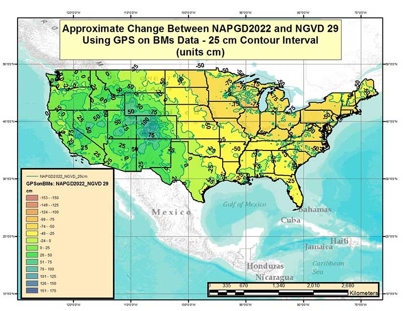
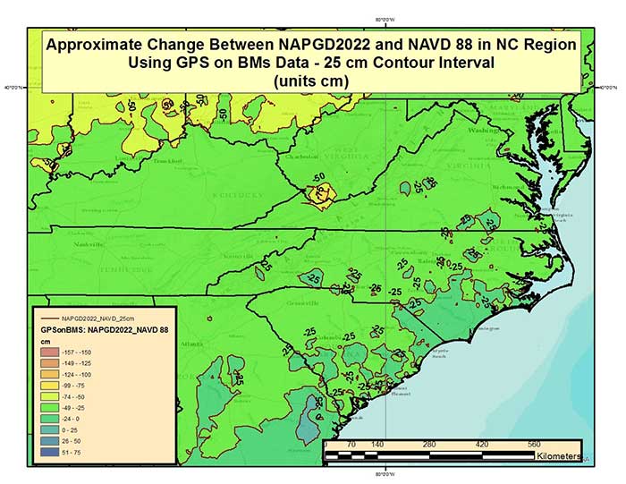
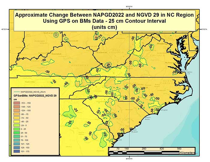
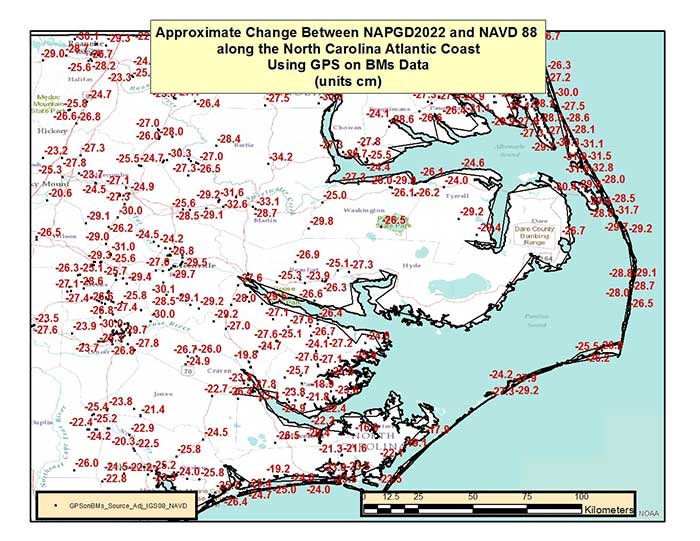
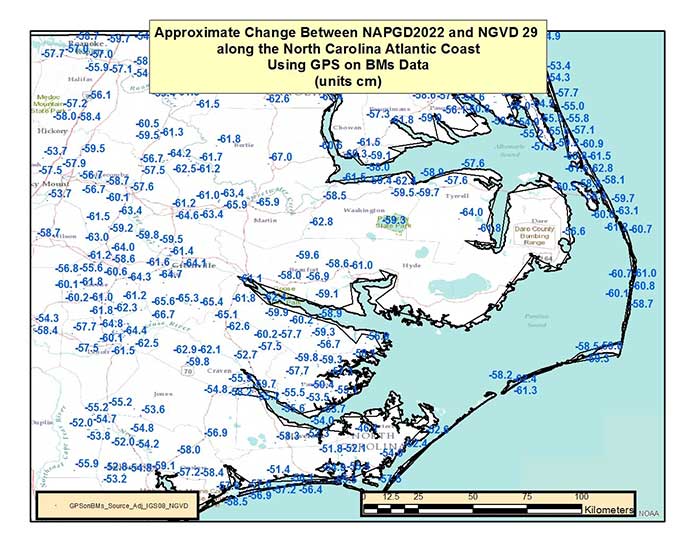
My last column highlighted two components of the North American-Pacific Vertical Datum of 2022 (NAPGD2022) — the geoid undulation model of GEOID2022 and gravity model of GRAV2022. It expressed that these two models will be very important to future surveyors and mappers that are incorporating geodetic data into NAPGD2022. The last column also emphasized the significant differences between NAPGD2022 and the U.S. National Vertical Datums of NAVD 88 and NGVD 29. A year ago, my February 2017 column provided information on strategically occupying benchmarks to support NGS 2017 GPS on BM Program. The column focused on addressing the following questions: (1) Is the large GPS on BM residual due to an issue with the NAVD 88 orthometric height or the NAD 83 (2011) ellipsoid height? and (2) Should stations with large GMS on BM residuals be included in the development of NGS’ hybrid geoid models? The column provided suggestions on how users can assist NGS in determining the reason for the large difference between the modeled hybrid geoid value and computed GNSS/leveling geoid computed value. My October 2016 column demonstrated how to use the GPS on BMs dataset to identify potential issues in published NAVD 88 and NAD 83 (2011) heights. It focused on analyzing the NGS’ GPS on BM data set that was used to create NGS’ GEOID12B hybrid geoid model. It provided procedures that users could employ when analyzing the differences between the modeled geoid values and the computed geoid values using GNSS/Leveling data (GNSS-derived ellipsoid height minus leveling-derived orthometric height). The October 2016 column provided several examples of large relative differences in residuals between neighboring stations.
It should be noted that many of these large GPS on BM residuals could be due to an invalid NAVD 88 published height because the bench mark moved since the last time the height of the bench mark was adjusted and published, and/or an undetected error in an ellipsoid height due to a weak GNSS project design. Either way, in my opinion, most of these stations with large GPS on BMs residuals don’t accurately represent a bench mark with a current NAVD 88 height (or what I call a valid NAVD 88 height). When performing a geodetic survey, these stations would be identified as bench marks with invalid heights when following the appropriate Federal geodetic survey guidelines, procedures, and specifications. These bench marks should not be used in the hybrid geoid model just like they would not be used in controlling geodetic surveys. NGS’ goal is to create a hybrid geoid model that is consistent with published valid NAVD 88 values. User participation in NGS’ GPS on BMs Program is critical to creating a hybrid geoid model consistent with a current NAVD 88.
Recently, NGS performed a detailed analysis of the latest GPS on BMs data file using the published NAD83 (2011) ellipsoid heights, NAVD 88 orthometric heights, and the latest experimental geoid model height, xGeoid17b, to compute a new set of GPS on BMs residuals. At this time, the analysis has only included the 48 conterminous States, District of Columbia, Puerto Rico, and Virgin Islands. These data included NAD 83 (2011) ellipsoid heights from all submitted GNSS projects and OPUS Shared results. The goal of the detailed analysis was to create a statistical ranking of the marks based on a quantitative analysis of the leveling and GPS data. The following attributes were considered during the analysis:
- Total number of GPS observations to and from the station
- Date of last GPS observation to and from the station
- Whether or not the GPS station has repeat baselines between closely spaced neighboring GPS on BMs stations
- Total number of times the mark has been leveled to
- Date of latest leveling
- Quality of leveling (single run; double run; or single run, double simultaneous)
The analysis of this data set was used to identify stations that should not be used in the creation of a hybrid geoid model or a NAPGD2022 Transformation tool. The stations identified as outliers and labeled as “Do Not Use” in a hybrid geoid model were based on issues associated with the NAVD 88 published orthometric height and/or the NAD83 (2011) ellipsoid height. I have described some of these issues in previous columns (August 2015 column, June 2016 column, October 2016 column and February 2017 column) so I won’t go into details in this column. NGS used the detailed analysis of the latest GPS on BMs dataset to: (1) generate a prototype hybrid geoid model to evaluate the residuals at stations not used in the hybrid geoid model, (2) confirm that the stations recommended for re-observations should be observed again, and (3) identify void areas that need additional observations.
Since GEOID12B was created, users have been instrumental in providing OPUS results on bench marks in areas NGS said that they needed additional stations. Saying that, NGS realizes that everyone is busy and has limited resources to collect GNSS data on bench marks to support the next hybrid geoid model. NGS has used the detailed analysis to prepare material to assist users on strategically occupying stations to help support the GPS on Bench Marks Program, and create a hybrid geoid model that accurately represents a current NAVD 88. To eliminate confusion of where NGS would like new observations, NGS’ material contains a specific list of stations that they would like occupied with GNSS during the 2018 GPS on BMs program. This column provides a summary of the latest details of NGS’ 2018 GPS on BMs campaign which will be used to create the next hybrid geoid model in 2019 (see box titled “Personal Communication received from Galen Scott, Project Lead of NGS’ GPS in BM Program.”).
Personal Communication received from Galen Scott, Project Lead of NGS’ GPS on BM ProgramIn early 2019, NOAA’s National Geodetic Survey (NGS) will replace GEOID12B with GEOID18, a new hybrid geoid model to deliver improved GPS-derived NAVD 88-equivalent orthometric heights. This new model will serve as the official means for obtaining NAVD 88-equivalent heights via GPS. It will be the last hybrid geoid model that NGS will create before NAVD 88 is replaced by NAPGD2022.NGS will use available GPS on bench mark data to create the new model. Recent analysis of existing GPS on bench mark data and a prototype of the new hybrid geoid model created using that data has highlighted areas where additional data is needed to either confirm or update the local relationships between the ellipsoid, orthometric, and geoid heights. This email provides a prioritized list of bench marks for which additional GPS data is needed to improve the hybrid model. Data submitted on these marks will also support the development of the transformation tools that will be developed as part of the transition to the new datums. Data to support the hybrid geoid model will be accepted through August 31, 2018. NGS will continue to accept data to support the transformation tools through 2020. New prioritized lists of marks to support the transformation tools will be made available over the next few years as analysis of data requirements progresses. For the marks included in the attached document, NGS is requesting support in two ways:
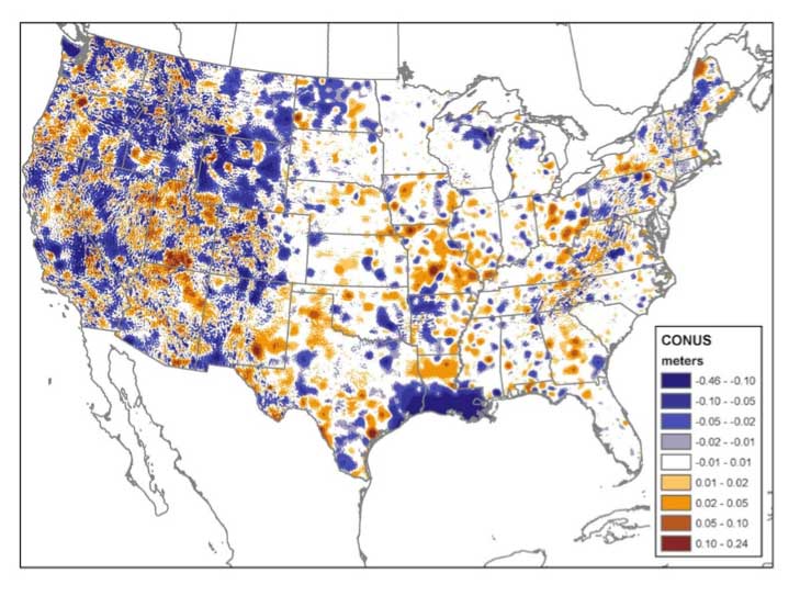
More information, including training material, is available on the NGS GPS on Bench Marks (GPS on BM) website. Two matching, independent GPS observations are required for each mark. The list indicates how many observations we have so far on each mark (obs_cnt column). A tracking map showing the currently prioritized marks and the number of observations we have on each will be added to the GPS on BM website in the near future. To maximize efficiency, please check this map before observing a mark to ensure that the required data has not already been submitted. Please note: Marks on this list may be inaccessible, destroyed, or not GPS’able. If this is the case, please locate and observe another nearby NAVD 88 mark, within ~10 km. The mark list is provided in three file formats, but all contain the same information, so choose the format you are most comfortable with: excel spreadsheet, esri shapefile, and Google Earth kmz. The image below shows the changes between GEOID12B and the prototype hybrid geoid model. While data is needed on all the marks in the list, you may further focus your data collection efforts by looking for areas in this image that show large changes in your region.
|
It is important for users to understand that NGS needs to have a high level of confidence that the OPUS Share results are accurate; therefore, they are requiring that “two matching, independent GPS observations are required for each mark.” The list of stations that they would like observed includes a count of the number of times that station has already been observed. NGS will be updating a website as stations are submitted so participants will not be wasting resources observing a station that has already been observed by someone else. It should be noted that if a station is only occupied once, it will still be useful for validating the hybrid geoid model; but stations occupied twice can be used in defining the hybrid geoid model.
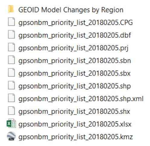
The attached file includes the list of stations that NGS would like observed to support the next geoid model. The information is provided in three different formats — excel spreadsheet, esri shapefile, and Google Earth kmz (See the box titled “List of Files for the 2018 GPS on BMs Program.”)
List of Files for the 2018 GPS on BMs Program
|
The data set also contains a folder titled “GEOID Model Changes by Region” which contains plots that depict changes between GEOID12B and the Prototype Hybrid Geoid Model (Note: at this time, NGS is denoting this prototype hybrid geoid model as GEOID18v2.2).
List of Files from Folder Titled “GEOID Model Changes by Region”
|
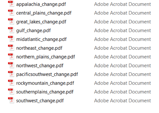
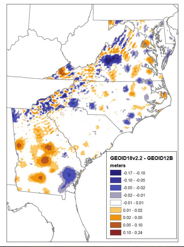
Figure 1 is a plot of the change between the prototype GEOID18v2.2 and GEOID12B in the Mid-Atlantic States. Looking at figure 1, the reader can see that there are some significant differences between the prototype hybrid geoid model values and the published GEOID12B values. On figure 1, all of the dark blue values are differences at the -10 cm level and the dark orange values are differences at the 10 cm level. There are several reasons for these changes including newly observed gravity data observations (especially in area with new GRAV-D data), improved data and models from satellites programs, new and improved algorithms for processing gravity data and estimating topographic effects, additional OPUS Share results in areas where GEOID12B didn’t have observations, and differences based on stations that were included in GEOID12B but rejected in the prototype model based on the latest detailed analysis.
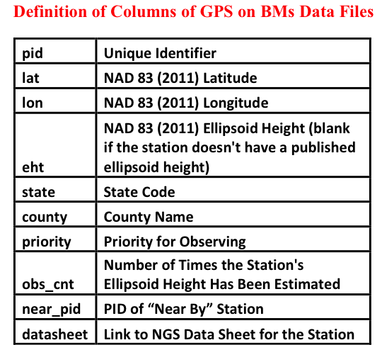
As previously mentioned, the list of stations that NGS would like observed with GNSS are provided in three formats: excel spreadsheet, esri shapefile, and Google Earth kmz. The box titled “Sample Data Elements Extracted from the Excel File Titled “gpsonbm_priority_list_20180205.xlsx” provides a sample of the data from the excel file. The box titled “Definition of Columns of GPS on BMs data file” provide the columns and a brief definition of the data field.
Sample Data Elements Extracted from the Excel File Titled “gpsonbm_priority_list_20180205.xlsx”
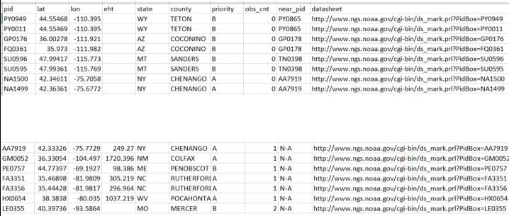
The priority column has two entries – A or B. Priority A is more important than priority B. In other words, if the user has to make a choice, NGS would like the priority A station observed first. The obs_cnt field will be updated as users submit their OPUS Shared results. Remember, NGS is requiring two matching, independent GPS observations for the station to be included in the development of the hybrid geoid and transformation tool.
The near_pid provides the pid of the station that is near the original station. The selection of the near_pid was based on the original station’s position and a search of the NGS database for a station within 5 to 15 kilometers of the original station. NGS’ analysis indicated that the original GPS on BMs station may have moved so an additional observation on the same station will not help to generate a hybrid geoid model that represents the current NAVD 88. It would warp the geoid model to fit the published NAVD 88 height but if the station moved since it was last leveled to, then it does not have a valid NAVD 88 height. As previously stated, when performing a geodetic survey, these stations would be identified as bench marks with invalid heights when following the appropriate Federal geodetic survey guidelines, procedures, and specifications. The surveyor would then level to another bench mark until they met the survey’s specifications. These bench marks with invalid heights should not be used in the hybrid geoid model just like they would not be used in controlling geodetic surveys. If the near_pid column is “n-a” then NGS would like the original station observed.
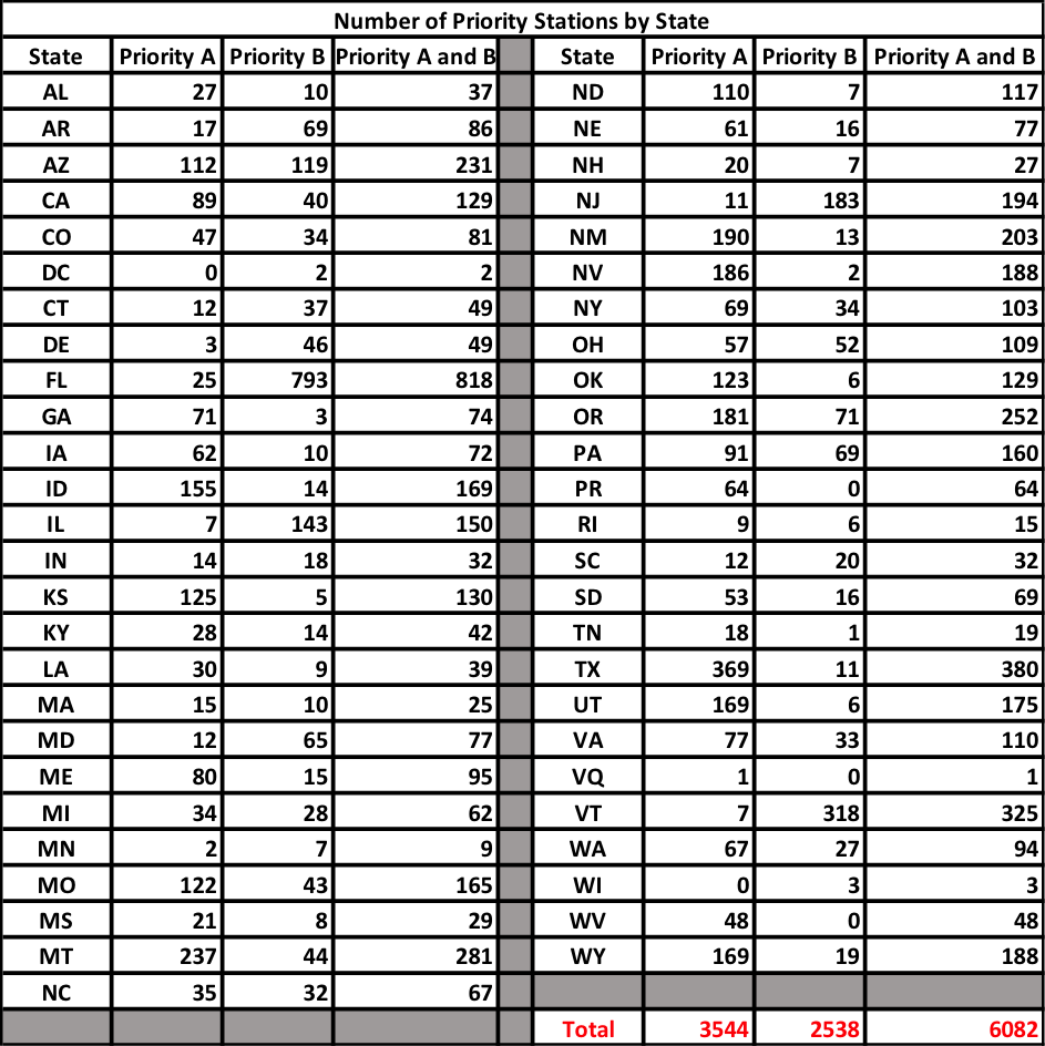
The box titled “Number of Priority Stations in Each State” provides the number of priority A and B stations for every State in the lower 48, the District of Columbia, Puerto Rico, and the Virgin Islands. Overall, there are 6082 stations in the list – 3544 Priority A stations and 2538 Priority B stations.
Number of Priority Station in Each State
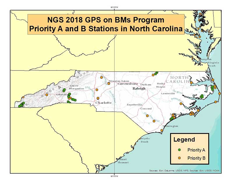
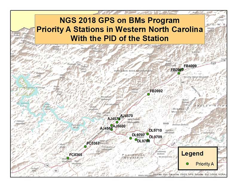
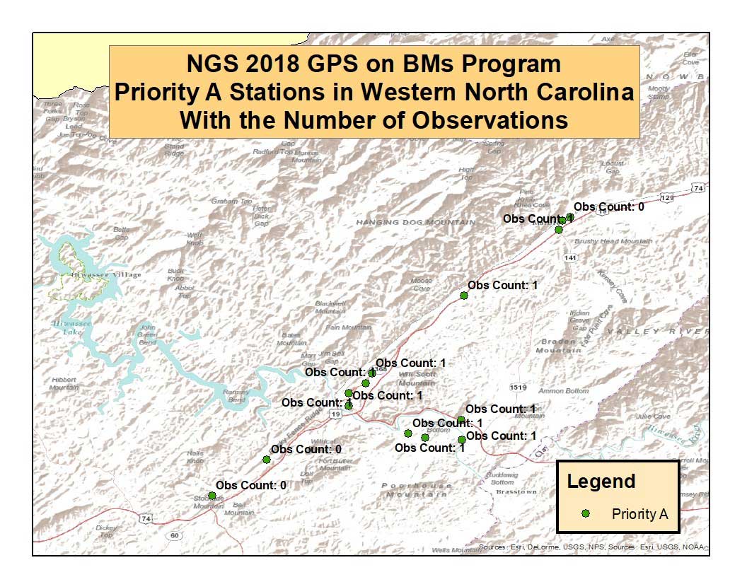
As an example of a State in eastern United States, the box titled “List of PIDs of Priority “A” and “B” Stations in North Carolina” provides the list of priority A and B stations that need to be observed in North Carolina. The box titled “List of PIDs of Priority “A” Stations in North Carolina” provides the list of priority A stations in North Carolina. Figure 2, titled “NGS 2018 GPS on BMs Program, Priority A and B Stations in North Carolina,” depicts the locations of these stations. Figure 3 depicts the location and PID of the priority A stations in western North Carolina. Figure 4 depicts the same stations with their Obs_Cnt value.
List of PIDs of Priority “A” and “B” Stations in North Carolina That Need to be Observed
Information extracted from Excel File Titled “full_priority_list.csv”
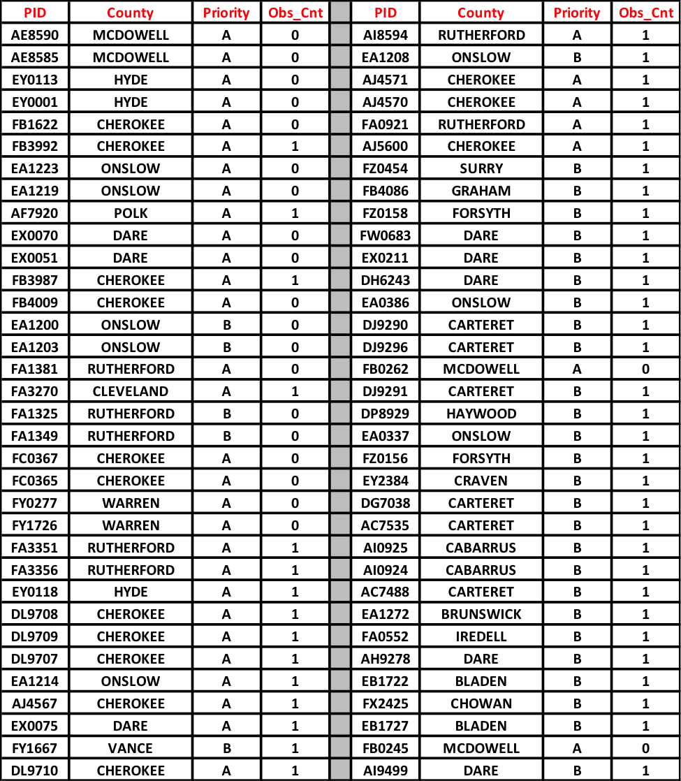
(Note: The stations in this table may not be the final list of priority A and B. The attached zip file contains the latest list of stations. The latest list was received too late to modify the table.)
List of PIDs of Priority “A” Stations in North Carolina
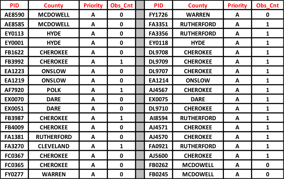
(Note: The stations in this table may not be the final list of priority A and B. The attached zip file contains the latest list of stations. The latest list was received too late to modify the table.)
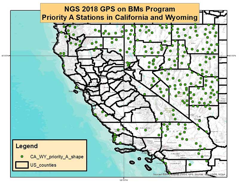
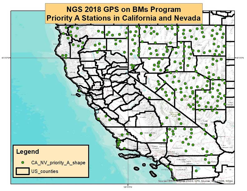
For completeness, I will provide an example of a region in the western United States – California and Nevada. They are larger States than North Carolina and have more Priority A stations that need to be observed. Figure 5 depicts the Priority A and B stations in California and Nevada, and figure 6 depicts the Priority A stations in California and Nevada. It is recognized by NGS that managing how these stations are observed and who does what is a monumental task. Some state agency may undertake observing all of the Priority A stations; for example, Gary Thompson, Chief of the North Carolina Geodetic Survey, has committed to observing all of the Priority A stations (personal communication). Other States have County and City surveyors that will help observe and manage the process. All of the information provided in the 2018 GPS on BMs allow individuals to sort the data in ways that meet their needs. For example, the box titled “List of Priority “A” Stations by County in California” provide the list of stations in California by county.
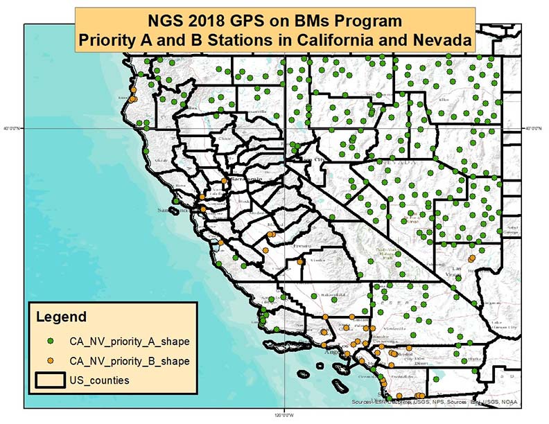
It should be noted that NGS identified the priority stations based on hybrid geoid requirements. The NGS geoid team would desire a valid GPS on BMs observation every 30 km. Therefore, some of the priority A stations are in areas void of any GPS on BMs stations. There may be many reasons for this but, most likely, it’s because it’s located in an unpopulated or mountainous region of the county. Either way, it may be difficult to obtain observations at these stations. The new hybrid geoid model will be created using whatever data are available. In these void areas, the geoid will be controlled by the nearest GPS on BMs stations. There is nothing wrong with this approach. The only issue will be that it will not be possible to evaluate the relation of the hybrid geoid model and NAVD 88 in these void areas. Figure 7 depicts the priority A stations and the population of cities in Northwestern Nevada and Northeastern California. The figure indicates that these priority A stations are located in an unpopulated region of Nevada. It’s obvious why there’s no GPS on BMs in this region since nobody lives there but the geoid doesn’t depend on population. In any event, if the user can obtain an observation in these regions it will really help in creating an accurate hybrid geoid model.
List of Priority “A” Stations by County in California
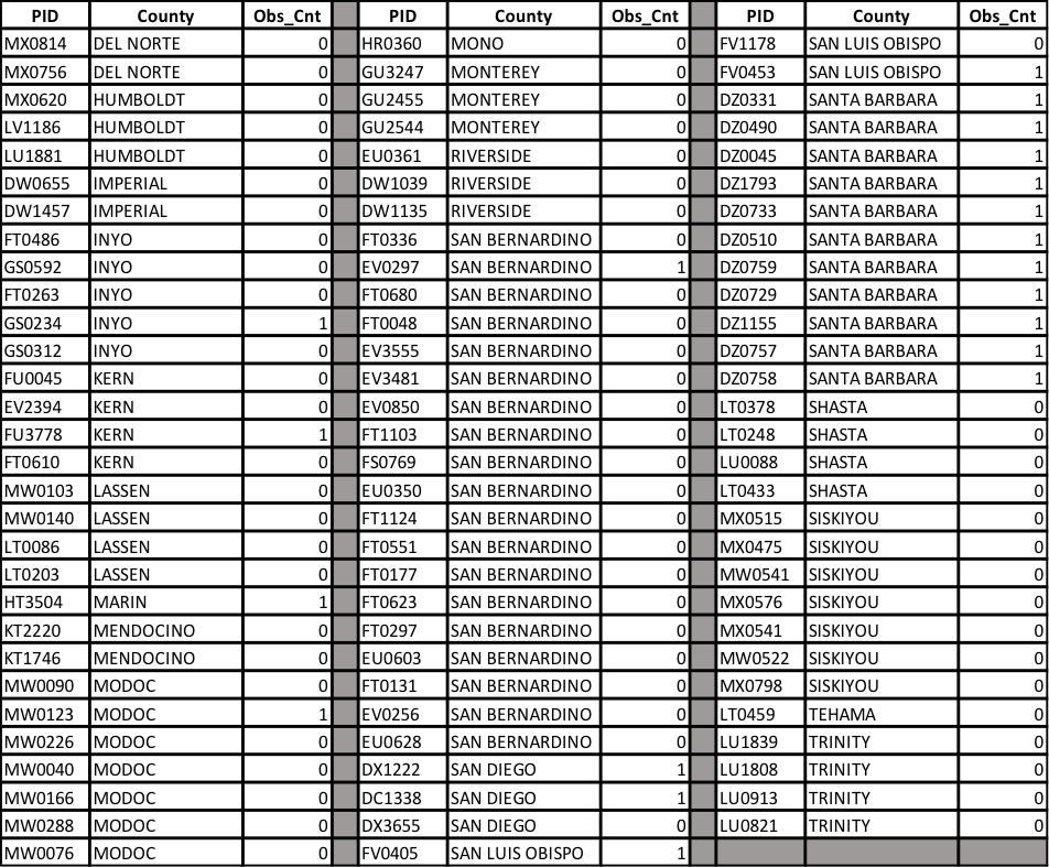
(Note: The stations in this table may not be the final list of priority A and B. The attached zip file contains the latest list of stations. The latest list was received too late to modify the table.)
NGS’ process for determining which stations were outliers and which stations should be re-observed involved analyzing both GNSS and leveling data from NGS’ database. The GPS on BMs residuals were computed using the procedure described in the box titled “Procedure for Computing the GPS on BMs Residuals.”
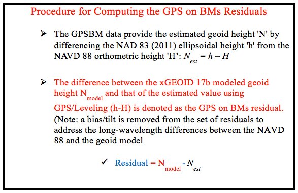
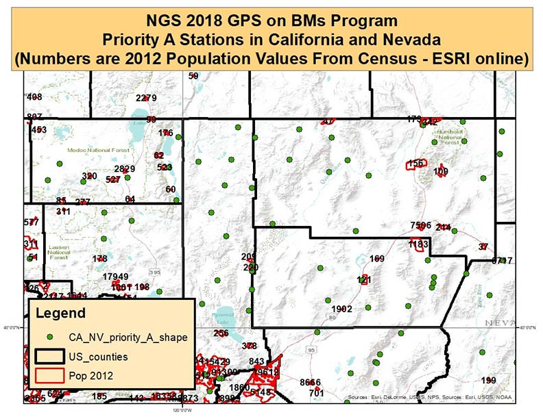
Figure 8 depicts the location of the GPS on BMs stations in Illinois. The box titled “Summary of Statistics for GPS on BMs Residuals in Illinois” provides a summary of the GPS on BMs residuals for the State of Illinois. The results indicate that there are 804 GPS on BMs in Illinois and the residuals range between -14.1 cm to 31.2 cm. They have a mean of 6.0 cm with a standard deviation of 4.6 cm. The table titled “Statistics for GPS on BMs Residuals in Illinois With Rejections Removed” indicates that most residuals fall between 2 and 10 cm. The box titled “Summary of Positive and Negative Statistics for GPS on BMs Residuals in Illinois” provides a summary of the statistics for the positive and negative set of residuals.
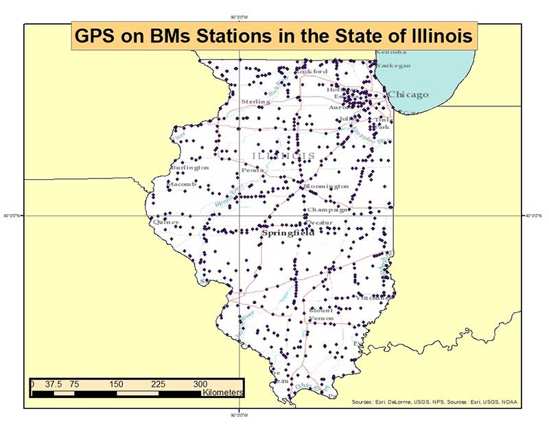
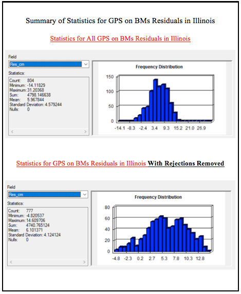
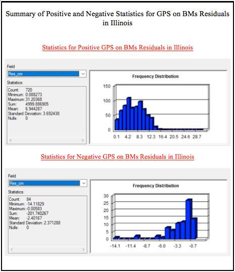
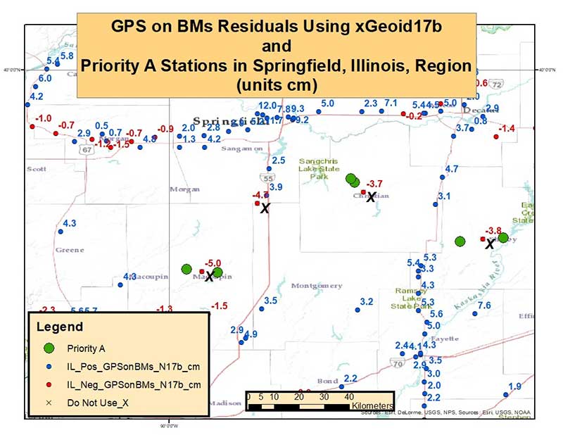
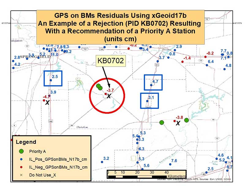
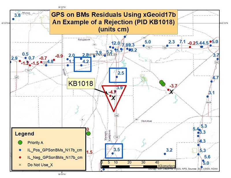
Figure 9 depicts the GPS on BMs residuals in the Springfield, Illinois, Region. During the detailed analysis of the latest GPS on BMs dataset, the analysts identified outliers that appeared to be large relative to their neighbors. Figure 9 depicts these outliers with a “X.” Stations designated with a “X” are stations that were designated as DO NOT USE in the creation of the hybrid geoid model. Figure 9 also indicates were the analyst recommended that a station should be observed before the creation of the next hybrid geoid model. These stations are labeled as Priority A stations on figure 9. Figure 10 is an enlargement of the same area that depicts a station that was recommended to be rejected in the hybrid geoid model (PID KB0702). The stations surrounding PID KB0702 all seem to be consistent with each other (residuals in smaller blue squares) so the analyst recommended that station KB0702 be rejected. At the same time, by rejecting this station, this creates a void area that needs to be filled. Therefore, the analyst also recommended that a new station be observed here; hence, the two priority A station plotted near the rejected station. Figure 11 is a plot of another rejected station (KB1018) in the same region but, in this case, the analyst did not recommend an additional observation in the area because there was another nearby station (station in red triangle) that was consistent with its neighbors (residuals in smaller blue squares).
As previously mentioned, and provided in the box titled “Attributes Considered During Analysis,” several attributes were analyzed before making the recommendations but, typically, GPS on BMs residuals between +/- 5 cm were used to identify which stations needed to be investigated.
Attributes Considered During Analysis
➢ Total number of GPS observations
➢ Date of last GPS observation
➢ Whether or not the GPS station has repeat baselines
➢ Total number of times the mark has been leveled to
➢ Date of latest leveling
➢ Quality of leveling
This analysis is the first cut at identifying stations that should not be used in a hybrid geoid model and providing a list of specific stations that could help improve the hybrid geoid model. All new data received by the cut-off date of August 31, 2018, will be analyzed by NGS and, if appropriate, the results will be included in the next hybrid geoid model. This is a great opportunity to provide data that will help to improve the hybrid geoid model in your region. My next column will provide a status report on the 2018 GPS on BMs Program.


![[FIGURE 2]](https://stage.globalpositioningnews.com/wp-content/uploads/2016/12/Fig2-NAVD-88-NGVD-29-Datum-Shift-Contours.jpg)
![[FIGURE 3] Coast-to-Coast Height Differences in the National Geodetic Vertical Datum of 1929 General Adjustment – Plot A](https://stage.globalpositioningnews.com/wp-content/uploads/2016/12/fig3-NGVD-29-genera-adjustment.jpg)
![[FIGURE 4] Coast-to-Coast Height Differences in the National Geodetic Vertical Datum of 1929 General Adjustment – Plot B](https://stage.globalpositioningnews.com/wp-content/uploads/2016/12/fig4-NGVD-29-general-adjustment.jpg)
![[FIGURE 5] Large GPS on BMS Residuals Between Stations 20 km Apart at the NC/SC Border (Note: rejections by geoid team have been removed)](https://stage.globalpositioningnews.com/wp-content/uploads/2016/12/Fig5-GPS-BMs-20km-NC-SC.jpg)
![[FIGURE 6] Large GPS on BMS Residuals Between Stations 13 kilometers Apart in South Carolina](https://stage.globalpositioningnews.com/wp-content/uploads/2016/12/Fig6-GPS-BMs-13km-NC-SC.jpg)