If there were ever a time to sit back and reflect on things that have happened in the last calendar year, the year 2020 will be the poster child for the next few generations (at least I hope so…). Because of several things that have happened worldwide in the profession of surveying, let us take this opportunity to look back on a year that was filled with new equipment, emerging technology and government interaction that will have a lasting effect on our surveying horizon.
Look at all of these wonderful toys
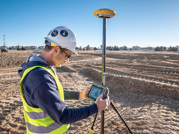
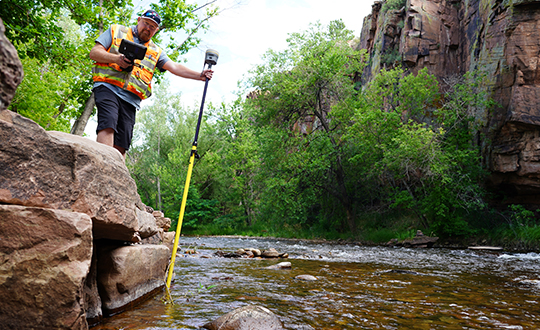
There was no shortage of introductions to new equipment for surveyors, especially in the GNSS receiver market. While combining GNSS capability with an inertial measurement unit (IMU) is not a new concept, the Big Three of Leica, Topcon and Trimble introduced new or upgraded versions of their latest receivers taking full advantage of the technology. The benefit of having the IMU integrated within the receiver is the ability to “tilt” the instrument yet having the calculated position remain at the tip of the receiver pole.
Leica, however, takes the tilting feature to another level with an integrated camera that allows for close-range photographs to capture additional information through remote sensing software. The data extracted from the photographs can be simple points (and verified in the data collector while in the field) or point clouds that can be integrated into larger projects through the Leica office software.
These new receivers, along with upgraded models from smaller providers, have opened the GNSS market to many more users well beyond surveying. The combination of more capability through advancing satellite constellations, more robust processors, and reduced receiver sizes have continued to drive GNSS positioning growth.

Manufacturers are using these increased capabilities to promote better coverage to obtain positions under heavier canopies and less likelihood for multi-path errors. While I remain cautious about these claims of increased coverage, I also maintain that with any tool, measurements and positions must have proper and appropriate validation. However, I am impressed that the technology continues to advance with what was once seen as only applicable to the open sky.
Not all the new technology has emerged through the GNSS receiver product lines; several less visible but valuable features have been introduced within the robotic total station lines. The manufacturers continue to push their equipment to react faster, stay locked on targets better, and provide more reliable solutions to data collection and construction layout. Data collectors continue to evolve with larger screens and more software capability, with some rivaling their desktop counterparts.
As cellular networks grow in both size and speed, more direct connections between field and office are being made with faster response time to data transfer. Data collection can take place in the field and be analyzed by an office technician as it happens. Go another step further and add an aerial background image to the collector and/or the office computer; now each team member can confirm that the information being collected is sufficient for the project in real-time.
Another technology that continues to advance is remote sensing, with more devices being introduced and with increased software capabilities. Besides new and upgraded offerings from the surveying-based manufacturers, other device makers are introducing products that offer remote sensing to the masses. The biggest news in this arena was the announcement from Apple that the iPhone 12 Pro and iPad Pro would come equipped with lidar sensing technology along with incredible photographic capabilities.
While there does not seem to be specific apps developed for surveyors at press time, it is safe to say that there will be in short order. It is also a safe bet that having this capability on a mass-produced device will put pressure on the surveying and mapping equipment manufacturers to be cost-competitive on their own proprietary devices or risk losing out on market share.
UAVs continue to be the fastest-growing segment of the surveying industry. More vehicle, sensor and software providers are coming to market to offer the surveyor a variety of choices. DJI continues to lead the way in the multi-rotor category with new products and sensors while other manufacturers are embracing the fixed-wing and vertical take-off and landing (VTOL) platform for greater range.
Just like their automobile brethren, flight time continues to increase with discoveries of new battery compositions and weight considerations. The sensor market is expanding to include more affordable lidar units, as well as new technology in multispectral identification, gas and noxious odor detection, and much more.
Software developers, too, continue to refine and expand the features found in their geospatial offerings with advancing technology and programming. Google Maps is the default navigation app for many smartphone users, but like anything utilizing GNSS in dense urban areas, the users find themselves bouncing all over the map.
While surveyors recognize this as multipath, the smartphone user does not have any way to remedy this trouble. Google recognizes this issue and has been working on a programming fix to help minimize these positional errors. This is another example of how precise position determination has become a significant goal for our society, with the more correct position, the better.
Meanwhile, in Washington D.C….
2020 did not see any shortage of government action for the surveying and mapping community. As with many topics that come out of the nation’s capital, it should not surprise anyone that several of the items considered by the federal government and its agencies were not without controversy.
The biggest and most controversial item continues to be the advancement of Ligado (formerly known as LightSquared) and the development of new communication technology that has been shown to interfere with the GPS transmission bands. The Federal Communications Commission (FCC), led by Chairman Ajit V. Pai, has been successful in holding off all challenges to the new technology including ones from current legislators and defense staff.
The main argument from the FCC is the value of the system as a provider of 5G communication to a substantial portion of the country. They also make statements that safeguards are being taken to protect the GPS spectrum, yet many studies from outside parties show otherwise. The fight over this spectrum will continue into 2021, and it will be interesting to see if the new administration will see things from a different perspective.
Several items to come out of Washington, D.C., late in the year were the blacklisting of DJI and the announcement of new UAV rules for flying over crowds and at night. With the DJI ruling, it is now illegal for government agencies to use the Chinese-based UAV maker for any activities. Based upon the significant market share of DJI, one can only wait to see how this situation plays out, and if the ban is expanded to private individuals.
The FAA announcement on the new UAV flight rules was surprising but not unexpected. In addition to establishing flight limitations over crowds and at night, it also established a timeframe for requiring most UAVs to transmit a Remote ID during flight for determining who is flying and where they are located. Compliance with these rules will be required by the manufacturer within 18 months and by UAV pilots within 30 months.
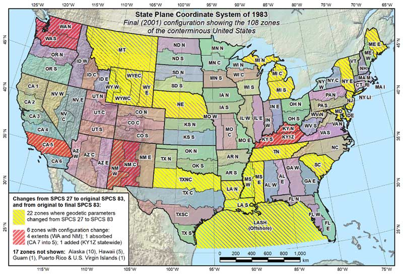
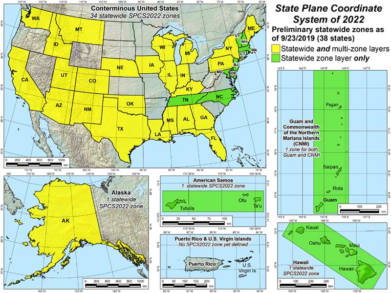
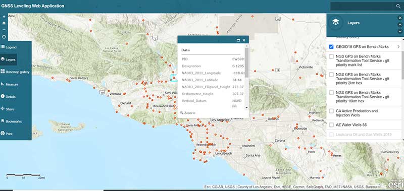
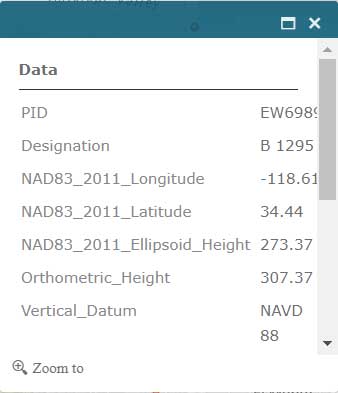
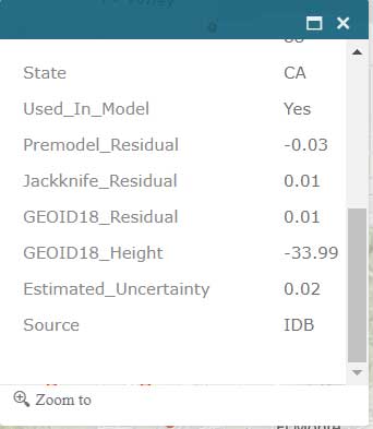
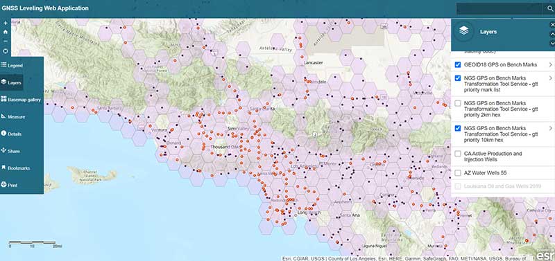
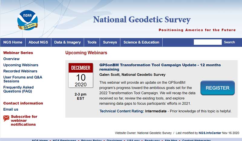
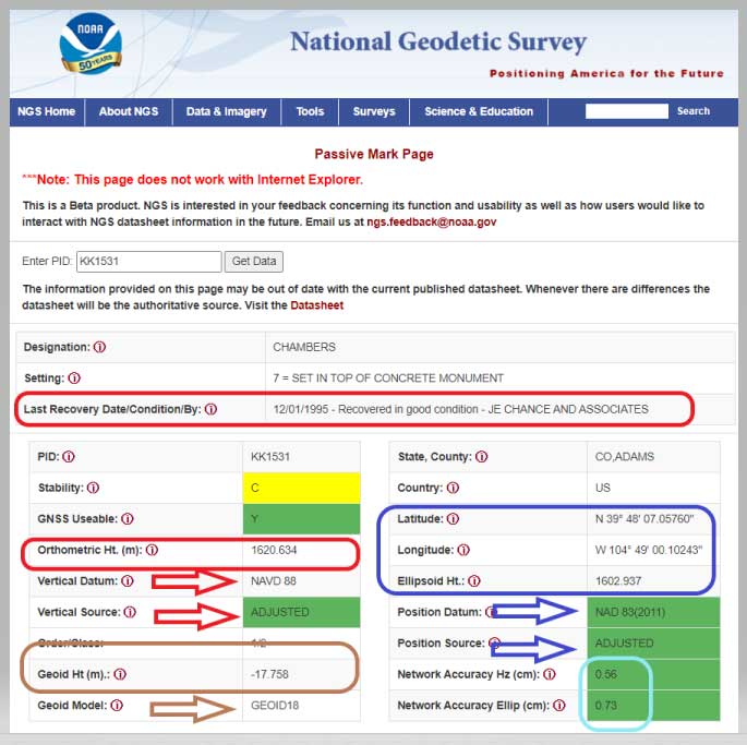
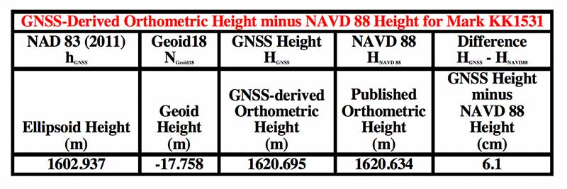
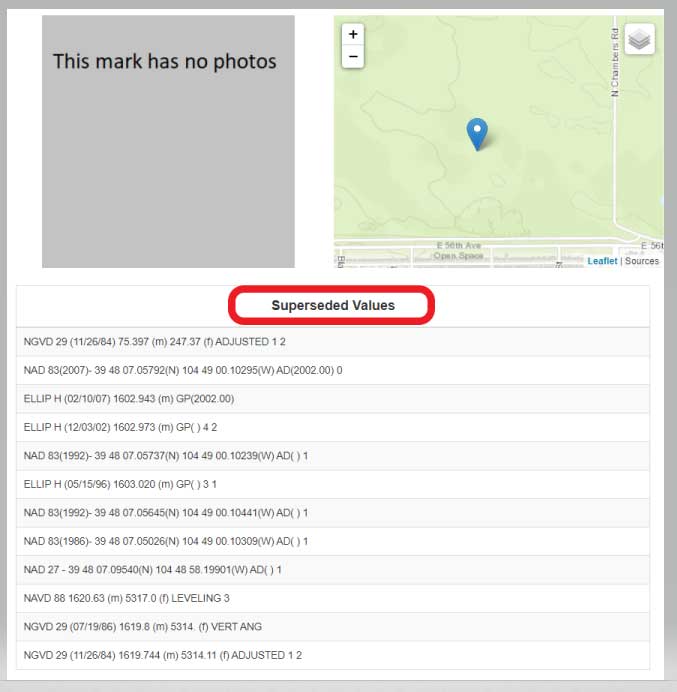
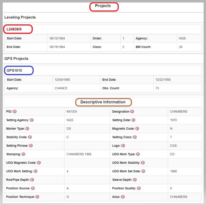
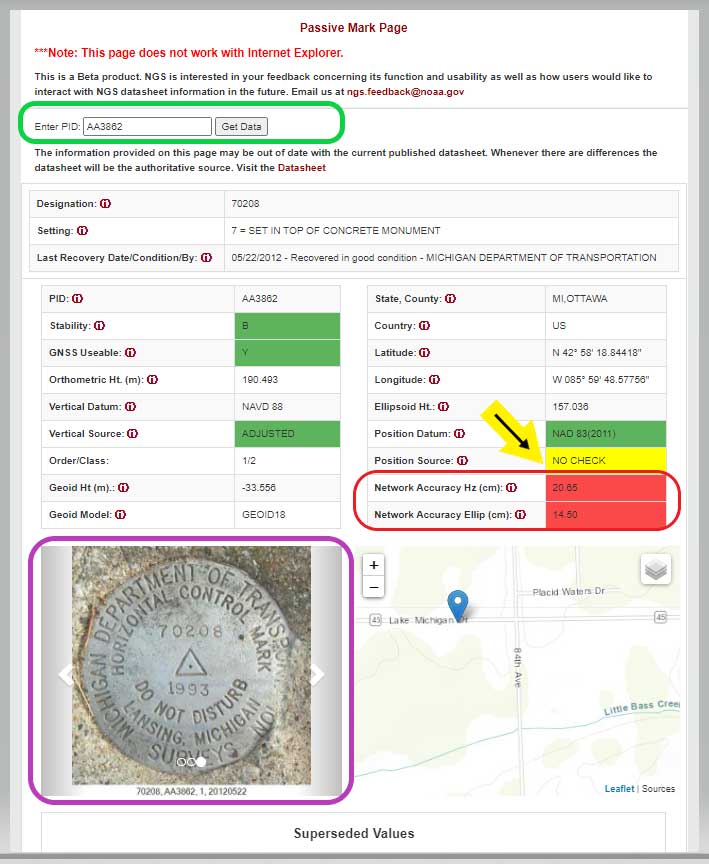
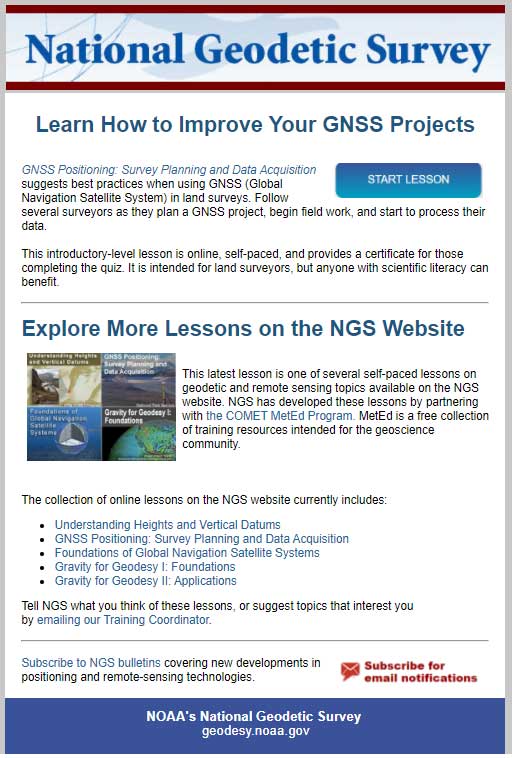
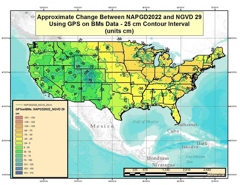
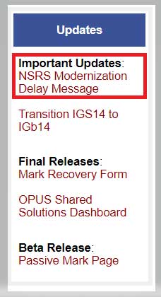
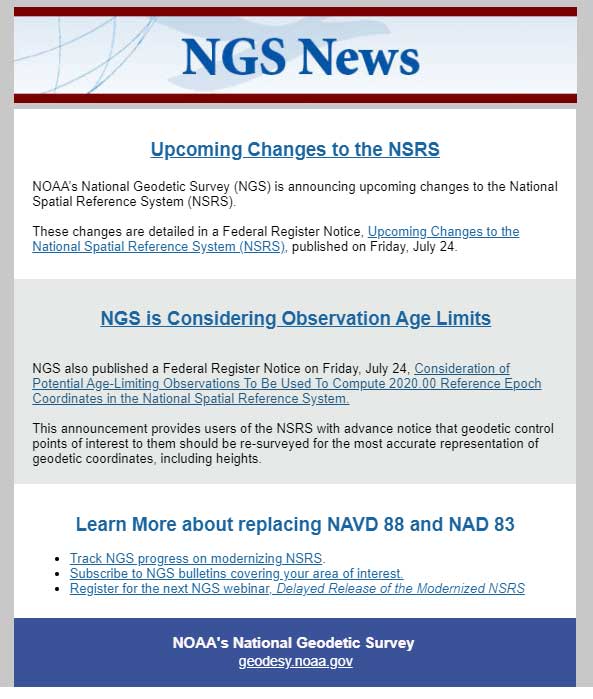
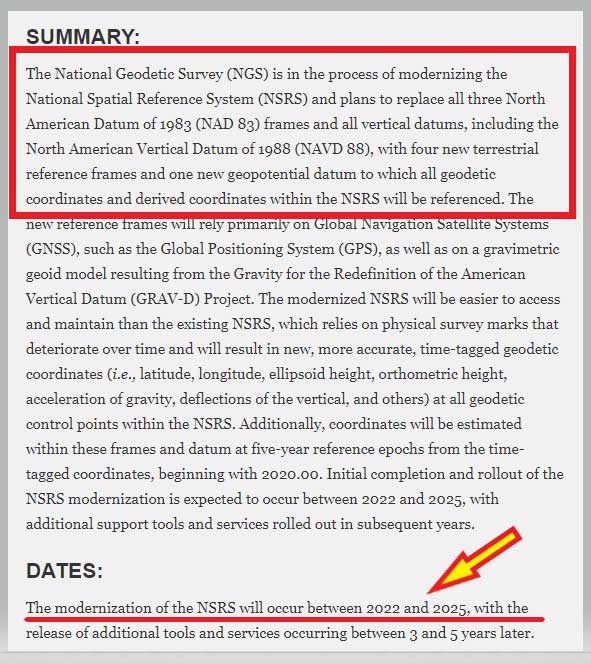
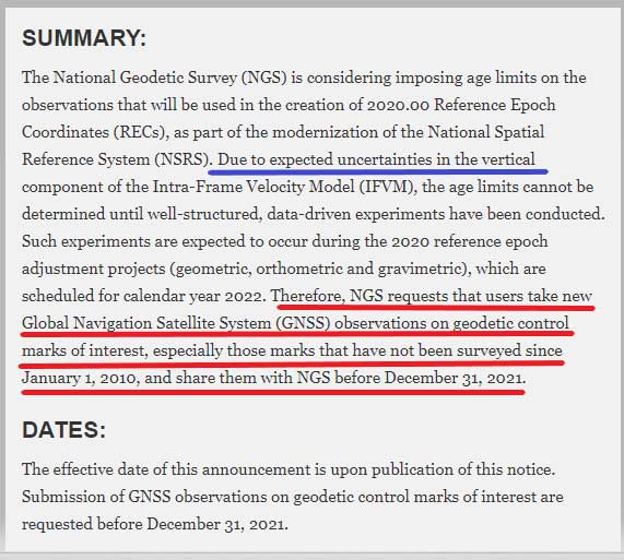
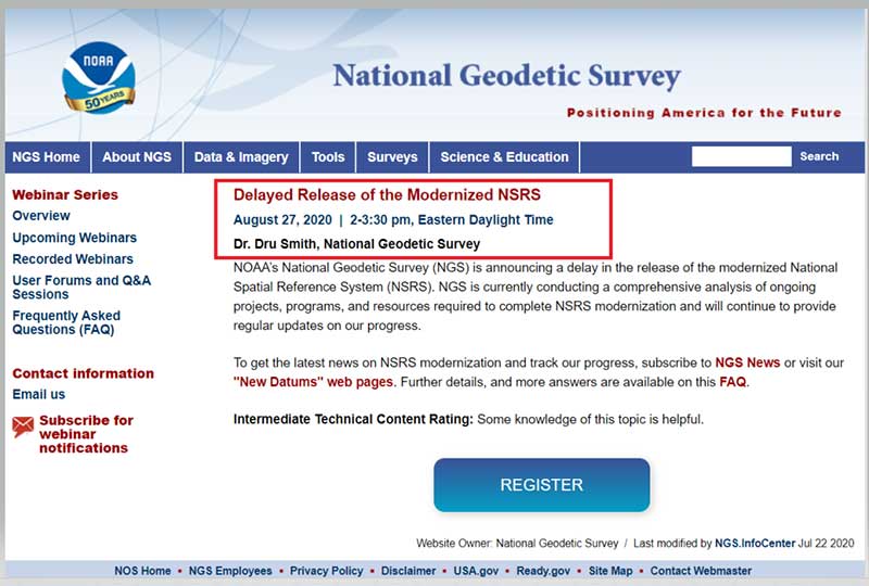
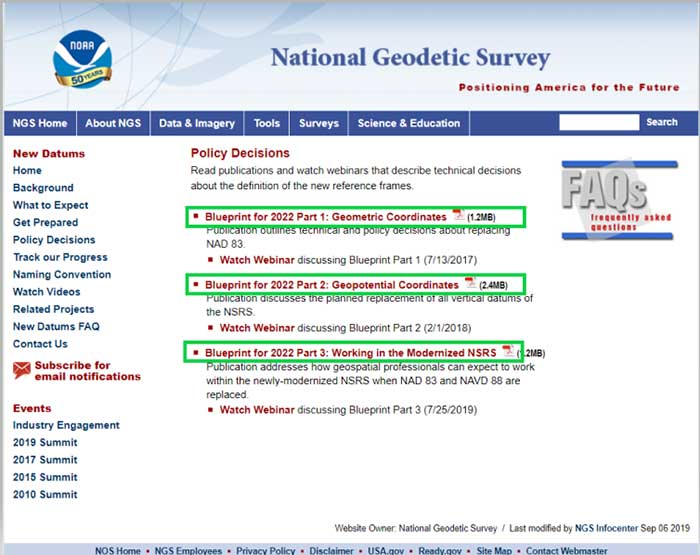
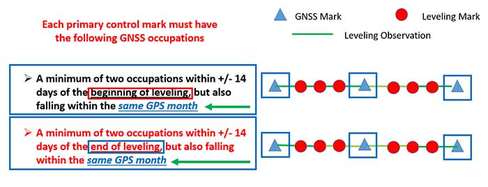
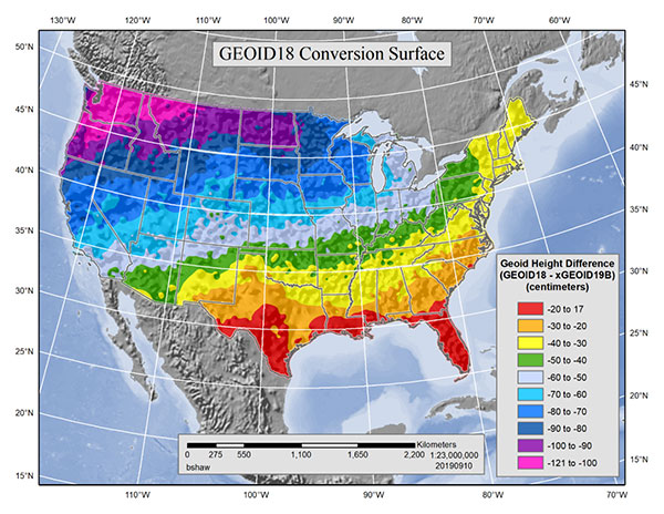
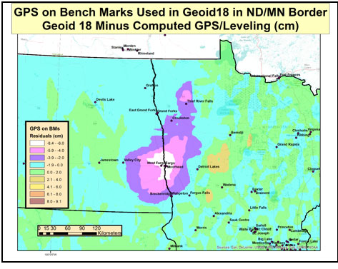
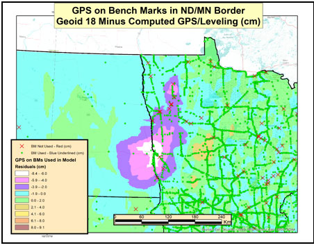
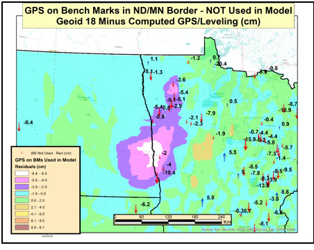
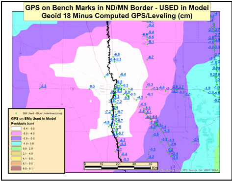
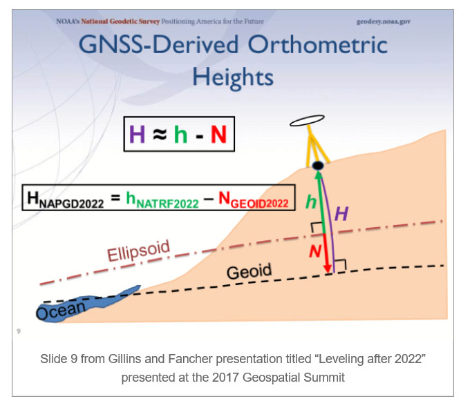
The National Geodetic Survey (NGS) has also been busy during 2020 preparing new datums and specifications for upcoming changes to the National Spatial Reference System (NSRS). Among those changes are the deprecation of the U.S. Survey Foot, beta testing of the latest geoid model (GEOID20), and new software tools for transforming positional information between datums. It was also announced that the release of the modernized NSRS scheduled for 2022 was being delayed.
NGS continues to work with each state on the improved state plane coordinate systems and/or low distortion projection systems that will be implemented with the new NSRS rollout. All these efforts have been a monumental task (no pun intended) and kudos go out to NGS for getting everything this far.
Pandemic 2020 (No, this is not a movie or a drill)
As we covered in the May 2020 Survey Scene article, COVID-19 was unlike anything we had been exposed before. Initial reports tried to relate the virus to typical influenza and the H1N1 outbreak in 2009, but the rapid transmission and sheer volume of cases (and deaths) mostly eliminated those comparisons.
From a technical viewpoint, the situation with COVID-19 has no bearing on GNSS operations and positional establishment. An operator of a GNSS receiver, and the business of surveying, is greatly affected by the presence of COVID-19 so it does deserve more than a brief mention in a retrospective look at the past year. This virus upended everything; from data collection and survey-related activities to computations and final drafting, the business of surveying felt the effects.
Once the initial challenges of keeping everyone safe were addressed, it became a year-long marathon of providing surveying services to clients that did not let the pandemic hinder their progress. Field crews were under significant pressure to maintain social distancing at every turn, while office staff dealt with home Wi-Fi and lack of access to normal business conditions such as large-format printing.
Video calls and instant messaging quickly became the norm, yet also became the scourge of dealing with the day-to-day operations of a business. The “normal” work/life balance with families, school, and social activities has disappeared and a more challenging approach has replaced that balance. Fingers are crossed that people will adhere to social distancing protocols and can get vaccinated as soon as possible so we can resume a portion of our previous lifestyles.
However, we do have several positive things to take away from the challenges of the pandemic that will make our lives better going forward. Our reliance on geolocation became quite clear throughout the pandemic. Whether it is using it to help establish contact tracing or as simple as having a delivery service bring necessities straight to your door, almost everyone relies on geolocation for helping guide them through the “new normal.”
We are using our smartphones to track our family members and help keep them out of harm’s way. It would be hard to imagine how much more difficult this situation would have been before cellphone and GNSS integration.

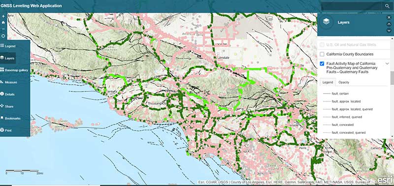
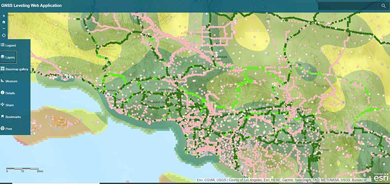
Another leap forward that most people are not aware of is the publicizing of GIS dashboards and incredible analysis of the geolocation of people worldwide. While GIS dashboards have been in existence for many years, it is only now that the public has paid attention to the vast information available to them.
From providing numbers of cases to graphically depicting “hotspots” across the world, these dashboards are full of useful information to help people understand the size of this pandemic, the places where mitigation is working, and where additional restrictions are being put in place to help reduce the spread of COVID-19.
The ability to merge geolocations with physical conditions and situations into a real-time mapping solution can help reduce the spread of the virus. By combining GNSS technology with advanced computing power and data storage, the power of GIS has been brought to the front page of public agencies and news sites.
While we still enjoy watching movies with superheroes, the true heroes during this pandemic are the frontline health workers, first responders and data analysts/programmers who bring us this timely information quickly. A hearty thank you goes out to all of them for their efforts and dedication to the cause.
In memoriam
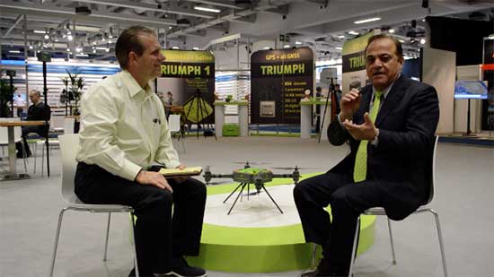
The year 2020 also brought losses to every corner of the world and the surveying community was not spared. There are very few individuals we call pioneers in the surveying industry, so to include Dr. Javad Ashjaee among that group is no small feat. His contributions to the surveying profession helped turn every practitioner into a geospatial information provider.
From his early days at Trimble pioneering the commercial-grade receiver to creating his company at Ashtech and embracing GLONASS with GPS, he continued to expand the capability of the GNSS receiver. Many surveyors today only know his name through his latest company, Javad GNSS, and the unique line of receivers and measuring devices and their distinctive green color.

Dr. Ashjaee was a big part of the GNSS revolution, so next time you starts up their receiver to collect survey data, take a moment to thank him. It was my pleasure to meet and interview him at the 2017 Intergeo trade show in Berlin to talk about his product line. I was also able to test-drive his incredible GNSS products for a feature in GPS World magazine on using smartphones for data collectors.
To say the man will be missed is a big understatement and I wish his family well on continuing his company and tradition of making great leaps in technology.


![Figure 16: Difference between NGSGN and IGSN71 AG values [mgal] (Source: National Geodetic Survey)](https://stage.globalpositioningnews.com/wp-content/uploads/zilkoski-december-2019-column-image-14.jpg)
![Figure 28: GRACE Trend over Alaska from UTCSR RL06 GRACE Model [mm/yr] (Source: Figure 28 from Technical Report NOS NGS 69)](https://stage.globalpositioningnews.com/wp-content/uploads/zilkoski-december-2019-column-image-20.jpg)
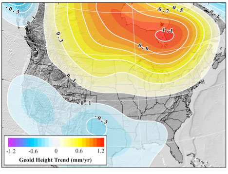
![Figure 32 From Technical Report NOS NGS 69: Geoid rate over CONUS based on the GSFC mascon model [mm/yr] (Source: Figure 32 From Technical Report NOS NGS 69)](https://stage.globalpositioningnews.com/wp-content/uploads/zilkoski-december-2019-column-image-21.jpg)
![Figure 33 From Technical Report NOS NGS 69: Geoid rate over Alaska from GSFC mascon model [mm/yr] (Source: Figure 33 From Technical Report NOS NGS 69)](https://stage.globalpositioningnews.com/wp-content/uploads/zilkoski-december-2019-column-image-22.jpg)