Tag: Oklahoma

3:13 a.m. Pulsing alarms. NOAA weather alert: TORNADO WARNING! TAKE IMMEDIATE SHELTER!

Without hesitation, the family awakened from their sleep, grabbed wallets, smartphones, car keys and hurriedly descended the stairs into the shelter. Doors sealed, the children crawled into their shelter beds.

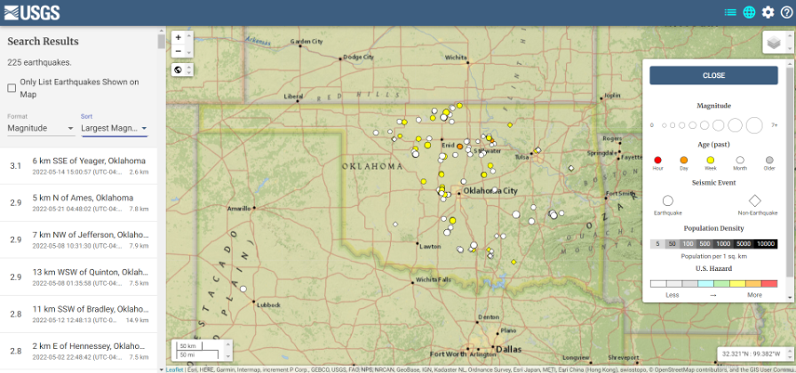
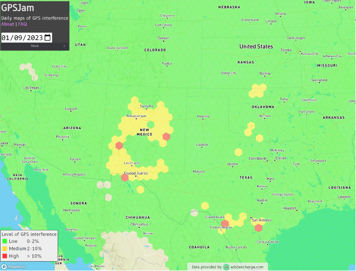
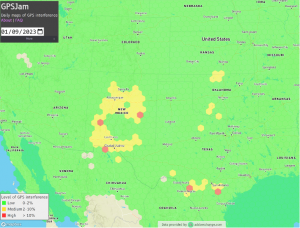
The mother and father, listening to the weather radio, heard their county’s name in the emergency broadcast. They looked at the smartphone’s weather map blinking with the text alert. A large swath of rain covered the area, painting yellows and reds inside a field of green. At the trailing edge of the storm, where skies were beginning to clear, the storm’s red tail began curling into a ball, moving directly toward them. Inside the ball, a dark red deepened into a growing magenta core. White pixels appeared within the magenta tail. Its path was unchanged and it was closing.

The man and woman huddled together watching the storm radar app on his mobile device not thinking about how their situational awareness is a confluence of spatial wizardry and atmospheric thermodynamics. The WSR-88D NEXRAD (Level III) radar scans a 143-mile radius, sweeping 14 elevation angles every five minutes to create a composite view of the surrounding weather. Colors correspond to the intensity of reflected hydrometeors (forms of precipitation) ranging from 0 dBZ, light rain in blue and green, to 75 dBZ, hail in magenta, and at 95 dBZ, it is physical debris carried aloft showing as white. Assembling the radars from across the country creates a seamless national weather mosaic (weather.gov/Radar). The dot on the smartphone’s weather app marking their own position is GNSS, orbiting far above.

In his hand both the NEXRAD and GNSS are blended in real-time as he watches the Tornado Vortex Signature (TVS) move toward his family and his house. Beyond the closed shelter doors, tornado sirens wail, mixed with peals of thunder. The warnings are no longer county names but names of towns. There are people for whom such a moment is not hypothetical. Scott Bagenzie knows exactly what comes next, not from imagination but from experience.

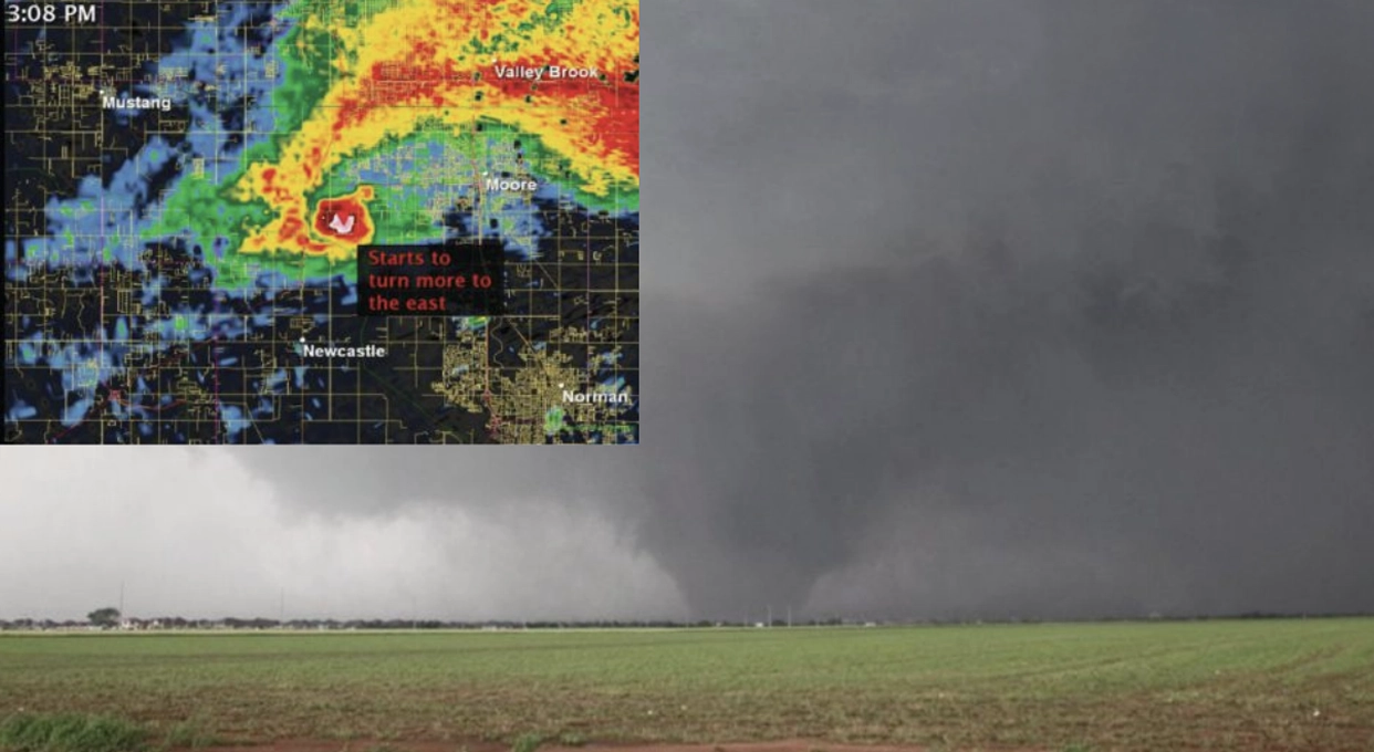
On Monday, May 20, 2013, at 2:56 p.m. Central Time, an EF5 tornado touched down northwest of Newcastle, Oklahoma, rapidly intensifying as it carved a path to Moore. The tornado lasted 36 minutes and covered 17 miles (FIGURE 1). Scott was caught by it, and I had the privilege of hearing him tell me what it is actually like to be inside those moments of sheer terror the rest of us only read about. He left work at 2:15 p.m. despite National Weather Service warnings for the counties flanking Oklahoma City. As he closed his car door, the sirens at the Mike Monroney Aeronautical Center went off. Security tried stopping him. He drove anyway.

“I was dodging cars left and right as people were taking pictures out to the southwest. I called Mari and said, hey, I’m running to the house to make sure the pets are taken care of. And she said, You crazy ***, take care of yourself.”

He pulled into his driveway, secured two cats in the closet and the dogs in the front bathroom, then stepped outside to see where the tornado was. His neighbor, who had an underground shelter in his garage, called out from next door: Get in over here! Scott went. As soon as the latch clicked behind them, debris began hitting the house above.

Weather as GIS

Weather is the most common topic of greetings. It is often the front page on newspapers. Television news is incomplete without a weather report, and weather is among the most downloaded apps on smartphones.

In many ways, the first GIS was weather, starting in the mid-1800s, long before computers, GNSS and GPS, hand-plotting data points, and then hand-drawing lines of equal pressure, temperature, humidity and winds on charts.

In the 1990s as a U.S. Navy weather specialist, I drew these charts by hand, plus four upper air charts learning how 3D spatial volumes interact. That was manual GIS. Now, in 2026, weather continues leading geospatial innovation via phased array radars, dual-pole radars (horizontal and vertical scans), acoustic atmospheric sensors, and predictive modeling for weather and climate, all of them layering atmospheric data using complex algorithms to forecast a dynamic fluid medium moving over an irregular spinning sphere that is unevenly heated. It is remarkably accurate, pushing the edges of geospatial predictive modeling.

The architecture of violence

The primary driver of powerful tornadoes is atmospheric thermodynamics unique to North America. Dry air crossing over the Rockies, cold arctic air pulled south by the jet stream, and warm moist air drawn north from the Gulf of America converge in a cauldron that can boil a normal convective storm into a sustained mesoscale supercell producing EF-5 tornadoes, the most powerful on record. Even though they make up less than one percent of all tornadoes, it is rare for EF5 tornados to occur anywhere else on Earth.

The Enhanced Fujita (EF) scale for measuring them was developed in 1971 by Theodore Fujita, a Japanese engineer whose forensic study of atomic bomb blast damage at Nagasaki and Hiroshima led to his damage-based framework for measuring tornado intensity.

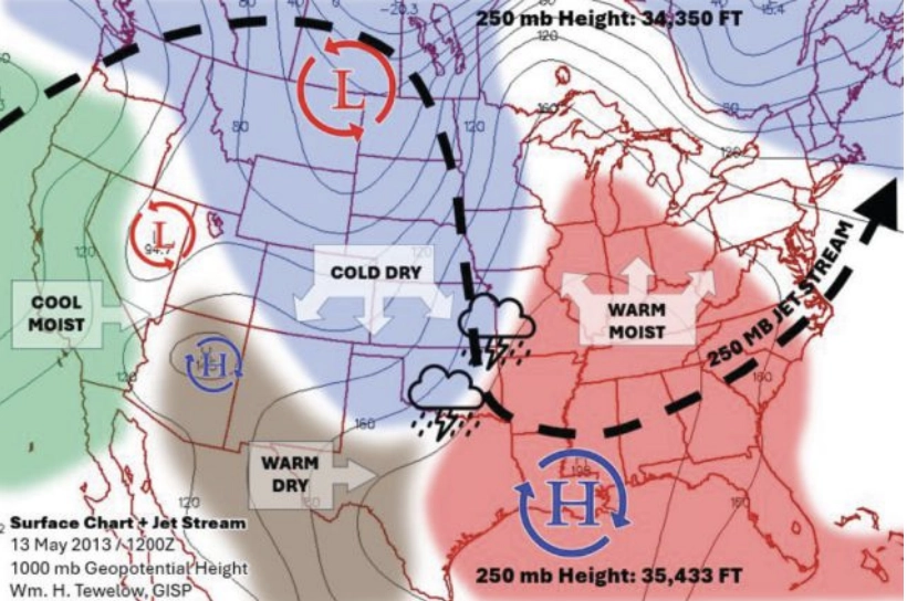
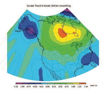
The jet stream, a river of air riding a thermal pressure gradient in the upper atmosphere, creates vorticity as cold dense arctic air plummets south, wedging beneath the warmer Gulf air and forcing it upward along the frontal boundary, before the jet stream curves back north. FIGURE 2, the 300 mb (mb stands for millibars of pressure) chart, shows this process has caused a low pressure over Texas sitting in a 1,200-foot-deep ravine. A jet streak will form as air rushes into the ravine increasing the jet stream’s speed, which draws in rising convection currents that can spawn mesoscale storm cells and set up the potential genesis of severe tornadoes.

When a funnel cloud forms, it is the visible physics of pressure dropping the temperature to the dew point causing condensation. The dropping pressure forms a bowl shape. Air flows into the dropping pressure, and the base of the cloud rotates cyclonically. As the rotation increases, centrifugal force of the colder dense rotating air pushes out the warmer higher-pressure air, further lowering the pressure at the core and deepening the bowl. That continues as the base descends into higher pressures at the surface, tightening the bowl into a cone. The difference in pressure between air outside the cone and what’s inside the vortex core can be 100 mb. That is basically a hole and wind rushes in to fill that void, but centrifugal force acts against the air. A tornado is born.

Wraiths of destruction

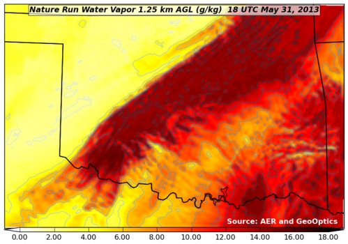
On May 31, 2013, 11 days after Moore, a multiple-vortex tornado formed near El Reno, Oklahoma. Along its periphery, small vortices spun around the rotating edge, circling, combining, breaking apart, vanishing and reforming, like wraiths of destruction dancing in a ring. The column darkened, descended and enveloped its own micro-vortices, forming the largest tornado ever recorded: 2.6 miles wide at its base.

It grew so rapidly that experienced TWISTEX storm chasers attempting to place instrument disks behind it were consumed as it expanded from 1.6 miles to 2.6 miles wide. A father, his son, and a colleague were killed; their car was found eight miles away.

Storm chasers are not thrill-seekers. WSR-88D NEXRAD, even at its lowest scan angle, already sits at 14,000 ft at its range limit because of the Earth’s curvature; spotters provide the ground truth radar cannot. Instruments such as Ground-based Local Infrasound Data Acquisition (GLINDA) extend that capability further: Tornadoes produce infrasound as low as 0.5 Hz, with a correlation between tornado size and frequency that may one day provide an early warning radar cannot.

I asked Scott whether he felt the tornado before he heard it.

“I couldn’t feel it,” he said, “but I could hear the sound of the train coming.”

I pressed him to describe it beyond the cliché. He thought for a moment, then said, “It’s not a cliché. That is what it sounds like. It sounds like a freight train, and the sound of the house being torn apart.”

The roar grows

Back in the shelter, the physics unfolded exactly as Scott described. Unaware of the sensation, a deep groaning sound resonates miles ahead of the tornado. A low constant roar grows louder as it approaches. Explosions pop as transformers blow. The shelter is pitch black except for the phone screen, that small glowing window showing a white ball of catastrophe moving toward them. The roar grows louder. Ears pop. Temperature drops. The house shakes. The roar of the freight train is so loud the screams inside the shelter cannot be heard. The doors rattle. The whirlwind is trying to break in. Then the roar fades, almost to silence, an eerie quiet.

In Scott’s shelter, the sequence was identical. His ears popped suddenly and painfully; they hurt for a full day afterward. In an EF5 tornado, pressure drops from roughly 950 mb in the surrounding air to 850 mb at the vortex core. The 100 mb passing over him was equal to a 3,000-ft pressure drop. It is the equivalent of instantly ascending two Empire State buildings stacked on top of each other, like falling straight up into the sky. Fighting against that force, Scott and his neighbor held shut the shelter latch as the doors bounced on their hinges.

“I don’t know how well those are constructed. I didn’t take any chances.”

Nearby, employees sheltering in a bank vault were physically holding the vault door closed as the tornado passed a thousand feet away. The vault’s timed lock could not engage. Five or six people leaned against a door designed to stop a robbery, fighting powerful thermodynamic forces.

Then Scott no longer had to hold the latch. The truck on the other side of the garage wall had been pushed against the hatch from outside, pinning them in. When they finally forced it open and stepped out. There was nothing.

“She just started screaming. She said, ‘No way, it didn’t do that.’ I told her, yeah, there’s nothing left.”

The entire event, from first debris strike to silence, lasted roughly one minute. At 28 miles per hour, a tornado traverses one mile in two minutes, plowing through a neighborhood in seconds.

Mapping the aftermath

The question the rest of us ask from a safer distance is: What is the true pattern of destruction across time and geography? To answer it, I built a Tornado Severity Index (TSI) using National Weather Service tornado data. On average, there are 970 tornadoes per year, 81% are EF0 and EF1; 18% are EF2 and EF3; and the catastrophic EF4 and EF5 make up 1%.

The NWS database reports the start and end coordinates, path width, magnitude, fatalities, injuries, and damages to property and crops. Working with the coordinate pairs, I calculated the distance and radial bearing of each path. But the EF scale alone tells only part of the story: A powerful tornado crossing an empty field and a moderate tornado crossing a dense neighborhood are not equivalent human events.

I did not want the TSI to be another version of the EF scale, so the weighting was based entirely on the human toll. The formula is total fatalities (F) at 100% plus injuries (I) at 10%, =F + (I x 0.1) and normalized on a scale of 1 to 100. Economic damage was originally part of the equation, but the data are inconsistent and unreliable across reporting jurisdictions.

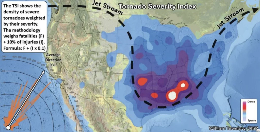
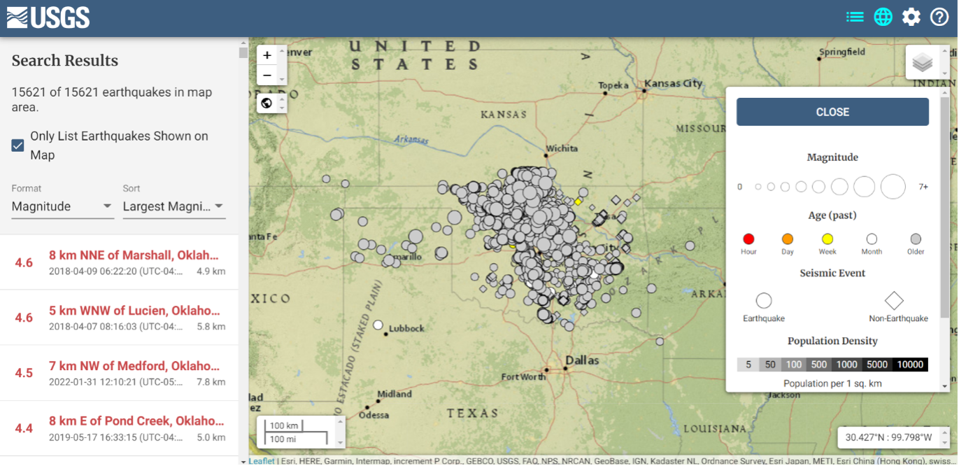
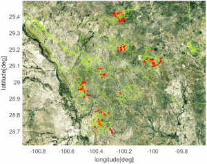
The resulting composite doesn’t measure the strength of tornadoes, but rather their human impact (see FIGURE 3). The dataset of tornadoes from 1950 to 2024 is 71,813. Filtering it down to those tornadoes that had a human consequence where the TSI>1 reduced it to 2,362 tornadoes. I reduced it further to 1,625 including only those with one or more fatalities. This was made into a heatmap. The data were further reduced to 301, only filtering out all except where TSI>10. The heatmap color scale was weighted to the TSI Score. It shows where the highest concentration of intense tornadoes occurs.

The results confirm Tornado Alley from Texas up through Oklahoma, and it also reveals Dixie Alley, an even more destructive corridor of severe tornadoes over Mississippi, Alabama and Tennessee. These areas align with the deep spring meridional jet stream discussed earlier. The northern side of the jet stream enhances cyclonic flow for storms in the area. The peak region of vorticity is where the jet stream turns back north again over Dixie Alley. Additionally, the rising terrain in that area causes orographic lifting and more rain, many times hiding the tornadoes within the pouring rain.

GIS reveals what the physics predict: a narrow corridor of atmospheric geometry where conditions for catastrophic tornadoes are optimized, running through the same communities, year after year.

For the sake of context, the Joplin, Missouri tornado on May 22, 2011, that caused 158 fatalities, 1,150 injuries, and damages of $2.8 billion ranks at the top of the TSI. The Moore tornado only scored 16.6 due to far fewer fatalities.

The dataset reveals the physical signatures of severe tornadoes. On average, they peak in mid-May at 5:30 p.m. with a strength of EF4.2, carve a path 36 miles long and 2,073 feet wide, and each one causes 13 fatalities, 173 injuries, and losses of $71.5 million. Severe tornadoes do not travel west. They do travel a spectrum where most of them fall within a range from 016° to 060° with an average path of travel northeast at 031°. This is why Scott was right to question the reports of the El Reno tornado tracking southeast: What appeared to be southward motion was lateral growth. The tornado was not moving south; it was becoming enormous.

“Pretty much sucking everything up,” Scott said, with confidence born out of his experience.

The pattern and the person

The TSI heatmap is a record of moments like Scott’s, representing a convergence of humans caught up in brutal atmospheric physics, where air becomes violent. The science explains the experience. It cannot prevent the next EF5; the thermodynamics will prevail.

What GIS adds is pattern, memory and prediction. The TSI with directional analysis gives emergency managers, planners and underwriters insights for understanding where storm physics and humans intersect most acutely, and therefore where shelter codes and warning systems must be most robust.

The family in their shelter, watching the white dot approach on the glowing screen, is experiencing the culmination of decades of geospatial and meteorological investment: NEXRAD networks, GNSS constellations, real-time data fusion in a consumer app. But as Scott will tell you, the most important instrument was the steel latch on the shelter door, and what mattered most was the neighbor who held it open for him as the tornado approached.

Tornadoes are Earth’s thermodynamic engines of absolute chaos.

“I’m not interested in tornadoes,” Scott told me. “Once burnt, you don’t play with the matches anymore.”

Scott moved out of Oklahoma in 2013. The science is fascinating. People press right up to the edge of it, but the experience when science becomes personal is sheer terror.

Live tracking tornadoes with GIS census tracts can know in real-time the impact on populations to immediately begin rescue operations, clean-up and recovery.

GIS cannot capture the whirlwind, but it can track the most violent of them: northeast at 031°, seven football fields wide for 36 miles.