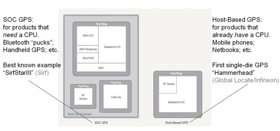
A one-chip multiconstellation GNSS receiver, now in volume production, has been tested in severe urban environments to demonstrate the benefits of multiconstellation operation in a consumer receiver. Bringing combined GPS/GLONASS from a few tens of thousands of surveying receivers to many millions of consumer units, starting with satnav personal navigation devices in 2011, followed by OEM car systems and mobile phones, significant shifts the marketplace. The confidence of millions of units in use and on offer should encourage manufacturers of frequency-specific components, such as antennas and SAW filters, to enter volume mode in terms of size and price.
One-chip GPS/GLONASS receiver trials in London, Tokyo, and Texas sought to demonstrate that the inclusion of all visible GLONASS satellites in the position solution, in addition to those from GPS, produces much greater availability in urban canyons, and in areas of marginal availability, much greater accuracy.
Multi-constellation receivers are needed at the consumer level to make more satellites available in urban canyon environments, where only a partial view of the sky is available and where extreme integrity is required to reject unusable signals, while continuing to operate on other signals deeply degraded by multiple reflection and attenuation. This article briefly outlines the difficulties of integrating a currently non-compatible system (GLONASS), offering an economic solution in the mass market where cost is king, but performance demands in terms of low signal, power consumption, time-to-first-fix, and availability are extreme. While the accuracy achieved is not at survey levels, we deem it sufficient to meet consumer demands even at the worst signal conditions.
The aim is to provide improved indoor and urban canyon availability for mass-market GNSS by using all available satellites; in 2011, that requires GLONASS support, as the constellation availability precedes Galileo by around three years. The aim is to overcome the hardware incompatibility issues of GLONASS, that is, its frequency division multiple access (FDMA) signal rather than the code division multiple access format used by GPS, different centre frequency, and different chipping rate, all without adding significantly to the silicon cost of the receiver chipset. This then allows a total satellite constellation of about 50 to be used at present, even before two recently launched Galileo IOV satellites.
It is expected that in benign conditions the additional satellites will give little benefit, as availability approaches 100 percent, and accuracy is excellent, with GPS alone. Though dominated by the ionosphere, using seven, eight, or nine satellites in the fix minimises the amount of error that feeds through to the final position.
In marginal conditions, where GPS can give a position, but is using 3/4/5 satellites and those are clustered in the narrow visible part of the sky resulting in poor DOP values, the increased number of satellites benefits the accuracy greatly, due to both improved DOP and multipath-error averaging. Limited satellites mean the full multipath errors map into position and are magnified by the DOP. Adding the second constellation means more clear-view satellites for accuracy, more total satellites to minimise the errors, and the errors are less magnified by the geometry due to better DOP.
In extreme conditions, where insufficient GPS satellites are seen to give a fix, the additional GLONASS satellites increase the availability to 100 percent (excluding actual tunnels).
Availability is a self-enhancing positive feedback loop… if satellites are always tracked, even if rejected on a quality basis by the RAIM/fault detection and exclusion (FDE) algorithms, then they do not need to be reacquired, so become available for use earlier. If position can be maintained, then the code phases for obstructed satellites can continue to be predicted accurately, allowing instant reacquisition after obstruction, and instant use as no code pull-in time is required. Once availability is lost, the reverse applies, as wrong position means worse prediction, longer re-acquisition, and hence again less availability.
The extra visible satellites are very significant for the consumer, particularly — as for example with self-assistance where the minimum constellation is five satellites, not three to four — to autonomously establish that all satellites are healthy using receiver-autonomous integrity monitoring (RAIM) methods. Self-assistance has further major benefits for GLONASS, in that no infrastructure is required, so there will be no delay waiting for GLONASS assistance servers to roll out. The GLONASS method of transmitting satellite orbits is also very suitable for the self-assistance algorithm, saving translation into and out of the Kepler format.
Significance of Work
Previous attempts to characterize the multi-constellation benefits in urban environments have been handicapped by the need to use professional receivers not designed for such signal conditions, and by the need to generate a separate result for each constellation or sacrifice one satellite measurement for clock control. These problems made them unrepresentative of the performance to be expected from the volume consumer device.
This new implementation is significant in being a true consumer receiver for high sensitivity, fully integrated both for measurement and for computation. Thus fully realistic trials are reported for the first time.
Background
The tests were performed on the Teseo-II single chip GNSS receiver (STA-8088). A brief history: our 2009 product Cartesio+ already included GPS/Galileo, and the digital signal processor (DSP) design has been extended to include GLONASS also for Teseo2, the 2010 product. Test results with real signal data through FPGA implementations of the baseband started in late 2009, and with the full product chip in 2010.
The architectural design showed that the silicon could be implemented with only small additional silicon area. Changes to the baseband DSP hardware and software were small and were included in the next scheduled upgrade of the chip, Teseo2. The RF chip silicon requires much greater attention, duplicating the intermediate frequency (IF) path and analog-digtal converter (ADC), with additional frequency conversion and a much wider IF filter bandwidth; however, as the RF silicon area is very small in total, even a 30 percent increase here is not a significant percentage increase on the whole chip. As the design is for an integrated single chip system (RF and baseband, from antenna to position, velocity, and timing (PVT) solution), the overall silicon area on a 65-nanometer process is very small.
Commercially, it is new to include all three constellations in a single consumer chip. Technically it is new to use a pool of constellation-independent channels for GLONASS, though standard for GPS/Galileo. Achieving this flexibility has also required new techniques to manage differing RF hardware delays, different chipping rates, in addition to the coordinated universal time (UTC) offset and geoid offset problems already well known to the surveying community.
It is also very unusual to go direct to a single-chip solution (RF+baseband+CPU) for such a major technology step. The confidence for this step comes from the provenance of the RF and the baseband, the RF being an extension of the STA5630 RF used with Cartesio+, and the baseband being significant but not major modifications of the GPS/Galileo DSP used inside Cartesio+. 5630/Cartesio+ were proven in volume production as separate chips before the single-chip three-constellation chip starts production.
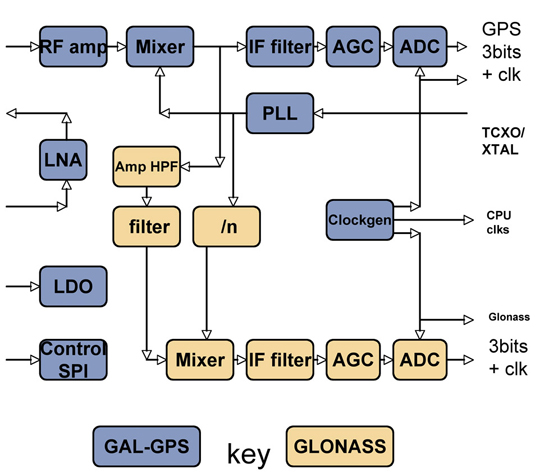
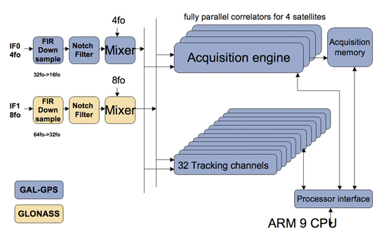
The steps forward from the previous generation of hardware are on chip RF, Galileo support, GLONASS support. While Galileo can pass down the existing GPS chain, with appropriate bandwidth changes, additional changes are required for GLONASS: see Figures 1 and 2.
Figure 1. RF changes to support GLONASS.Figure 2. Baseband changes to support GLONASS.
In the RF section, the LNA, RF amp, and first mixer are shared by both paths, in order to save external costs and pins for the equipment manufacturer, and also to minimize power consumption. Then the GLONASS signal, now at around 30 MHz, is tapped off into a secondary path shown in brown, mixed down to 8 MHz and fed to a separate ADC and thus to the baseband.
In the baseband, an additional pre-conditioning path is provided, again shown in brown, which converts the 8 MHz signal down to baseband, provides anti-jammer notch filters, and reduces the sample rate to the standard 16fo expected by the DSP hardware.
The existing acquisition engines and tracking channels can then select whether to take the GPS/Galileo signal, or the GLONASS signal, making the allocation of channels to constellations completely flexible.
Less visible but very important to the system performance is the software controlling these hardware resources, first to close tracking loops and take measurements, and secondly the Kalman filter that converts the measurements to the PVT data required by the user. This was all structurally modified to support multiple constellations, rather than simply adding GLONASS, in order that future extensions of the software to other future systems becomes an evolutionary task rather than a major re-write.
The software ran on real silicon in 2010, but using signals from either simulator or static roof antennas, where accuracy and availability of GPS alone are so good that there is little room for improvement. In early 2011, prototype satnav hardware using production chips, antennas, and cases became available, making mobile field trials viable.
Actual Results
Results have already been seen from trials using professional receivers with independent GPS and GLONASS measurements. However, those tests were not representative of the consumer receiver because they are not high sensitivity; because the receivers require enough clean signal to operate a PLL, which is not realistic in a mobile city environment; and because they were creating two separate solutions, thus needing a continuous extra satellite to resolve inter-system time differences.
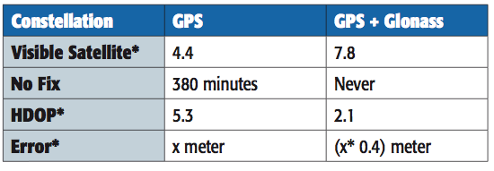
A 2010 simulation of visible satellites in a typical urban canyon of downtown Milan, Italy, produced the results, every minute averaged for a full 24 hours, shown in Table 1. The average number of satellites visible rises from 4.4 with GPS alone, to 7.8 for GPS+GLONASS, with the result that there are then zero no-fix samples. With GPS alone there were 380 no-fix samples, or 26 percent of the time.
Table 1. Accuracy and availability of GPS and GPS+GLONASS, averaged over 24 hours.
However, availability is not itself sufficient. Having more satellites in the same small piece of sky above the urban canyon may not be sufficient, due to geometric accuracy limitations. To study this, the geometric accuracy represented by the HDOP was also collected, and shows an accuracy 2.5 times better.
Previous studies suggested that in the particular cities tested, two to three additional satellites were available, but one of these was wasted on the clock solution. Using the high-sensitivity receiver, we expected four or five extra satellites and none wasted.
The actual results far exceeded our expectations. Firstly, many more satellites were seen, as all previous tests and simulations had excluded reflected signals. Having many more signals, the DOP was vastly improved, and the effect of the reflections on accuracy was greatly reduced, both geometrically, and by the ability of the FDE/RAIM algorithms to maintain their stability and down-weight grossly erroneous signals rather than allow them to distort the position.
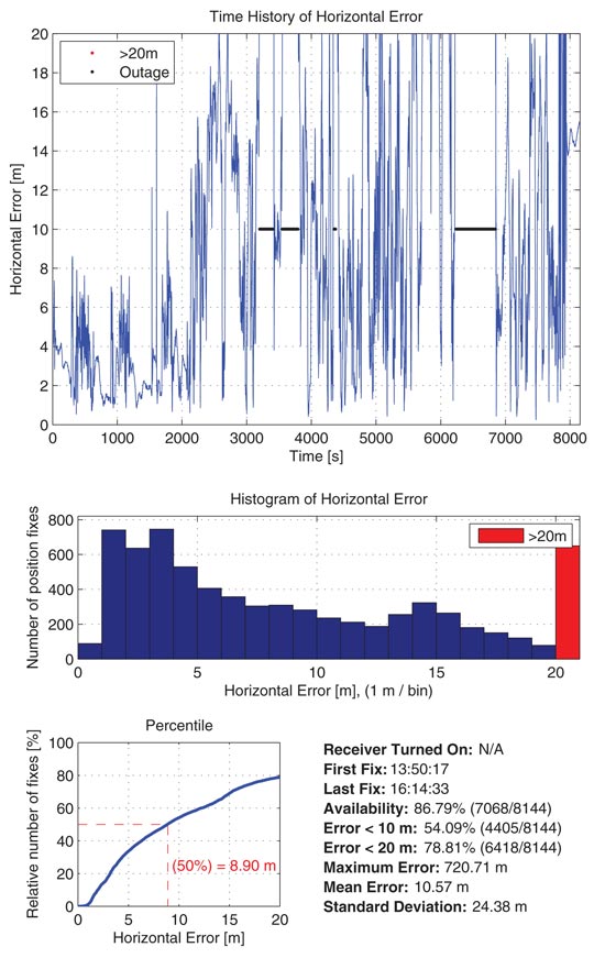
The results presented here are from a fully integrated high-sensitivity receiver optimized to use signals down to very low levels, and to give a solution derived directly from all satellites in view, no matter which constellation.
This produces 100 percent availability, and much improved accuracy in the harsh city environment.
Availability
The use of high-sensitivity receivers, not dependent on phase-locked loops (PLLs) for tracking, produces 100 percent availability in modern cities, even high-rise, due to the reflective nature of modern glass in buildings, even for GPS alone. Thus some other definition of availability is required rather than “four sats available,” such as sats tracked to a certain quality level, resulting in a manageable DOP. Even DOP is difficult to assess, as the Kalman filter gives different weights to each satellite, not considered in the DOP calculation, and also uses historic position and current velocity, in addition to instantaneous measurements, to maintain the accuracy of the fix.
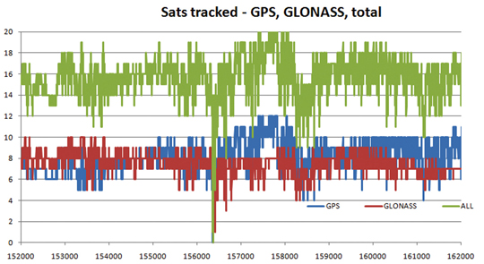
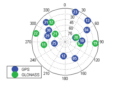
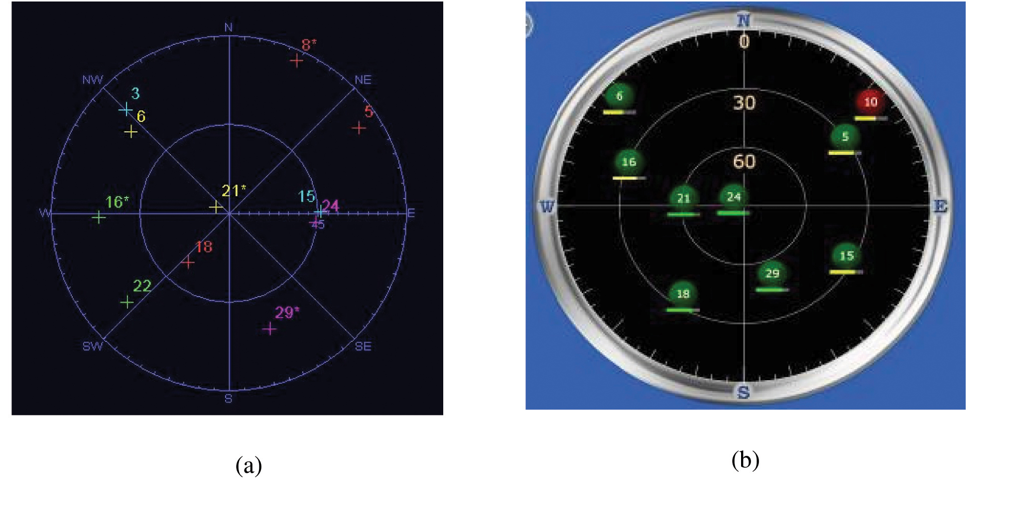
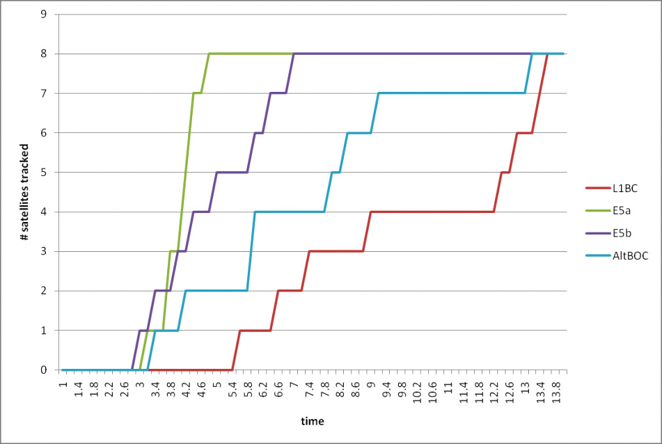
Figure 3 shows the availability of tracked satellites in tests in the London City financial district in May 2011.
As can be seen, there are generally seven to eight GLONASS satellites and eight to nine GPS satellites, for a total of around 16 satellites. The only period of non-availability was in a true tunnel (Blackfriars Underpass) at around time 156400 seconds. In other urban canyons, around time 158500 and 161300, individual constellations came down to four satellites, but the total never fell below eight. Note this is an old city, mainly stone, so reflections are limited compared with glass/metal buildings.
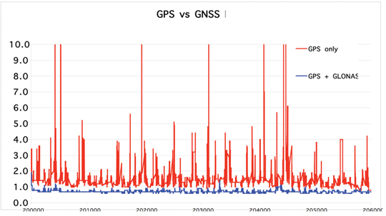
While outside tunnels, availability is 100 percent, this may be limited by DOP or accuracy. As can be seen in Figure 4 on another London test, the GNSS DOP remains below 1, as might be expected with 10–16 satellites, while GPS-only frequently exceeds four, with the effect that any distortions due to reflections and weak signals are greatly magnified, with several excursions over 10.
Figure 4. GPS-only versus combined GPS/GLONASS dilution of precision.
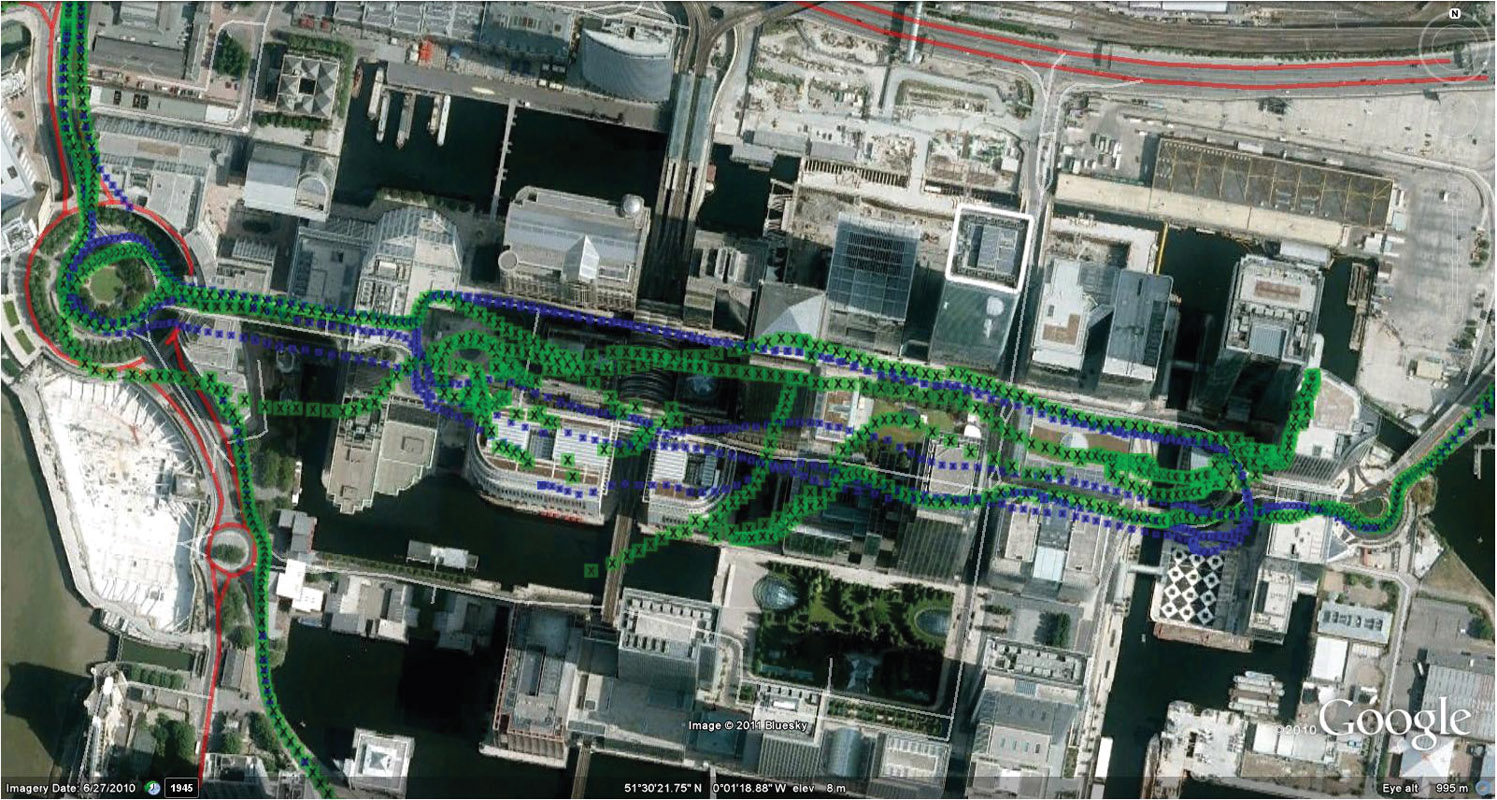
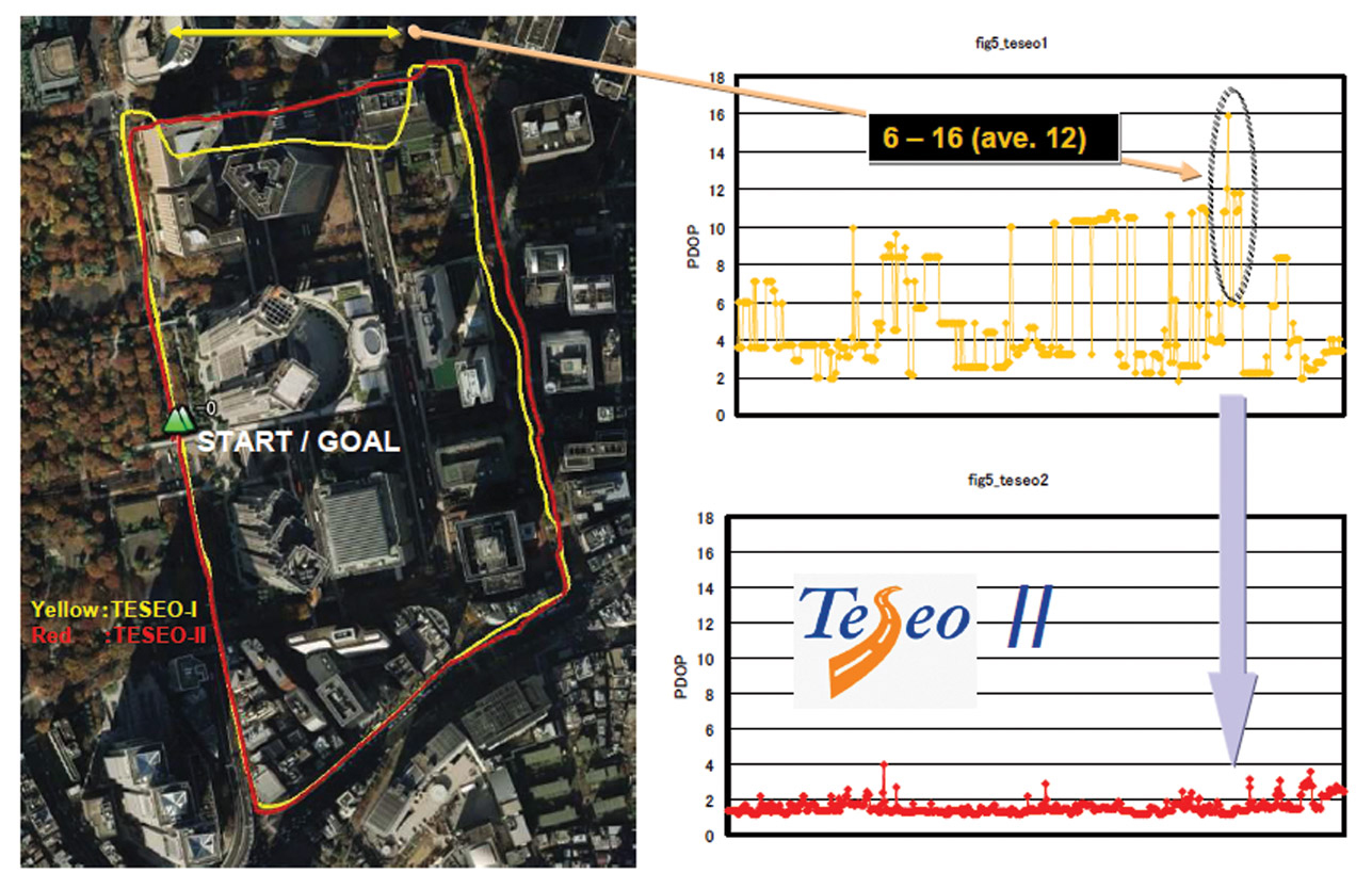
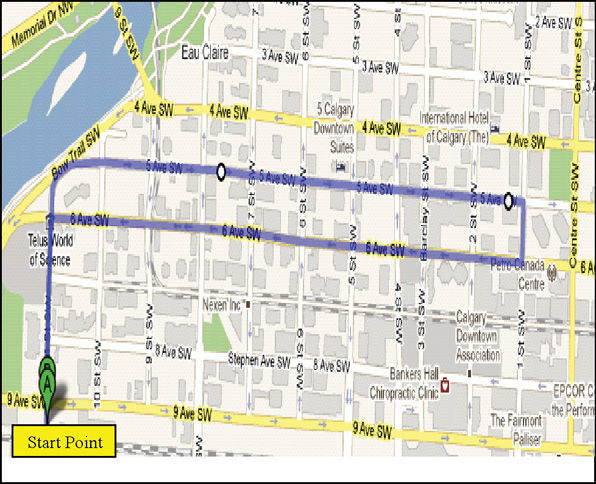
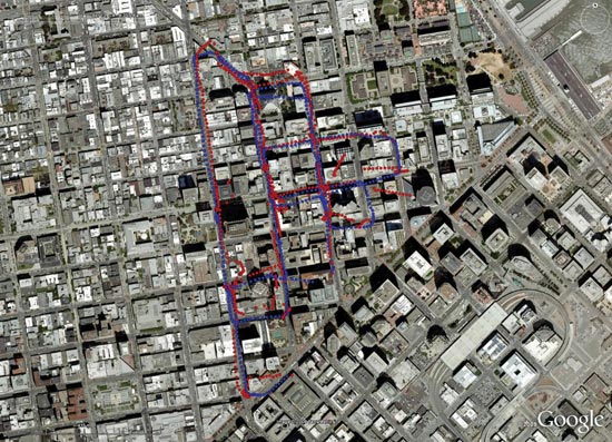
As the May 2011 tests had not been difficult enough to stress the GPS into requiring GNSS support, a further trial was performed in August 2011. This was in a modern high-rise section of the city, Canary Wharf, shown in Figure 5 on an aerial photograph. In addition to being high-rise, the roads are also very narrow, resulting in very difficult urban canyons. Being a modern section of the city, the buildings are generally reflective glass and metal, rather than stone, testing RAIM and FDE algorithms to the extreme.
Figure 5. GPS versus GNSS, London Canary Wharf (click to enlarge.)
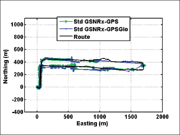
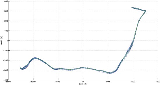
This resulted in difficulty for the GPS-only solution, shown in green, especially in the covered section of the Docklands station, center-left, lower track.
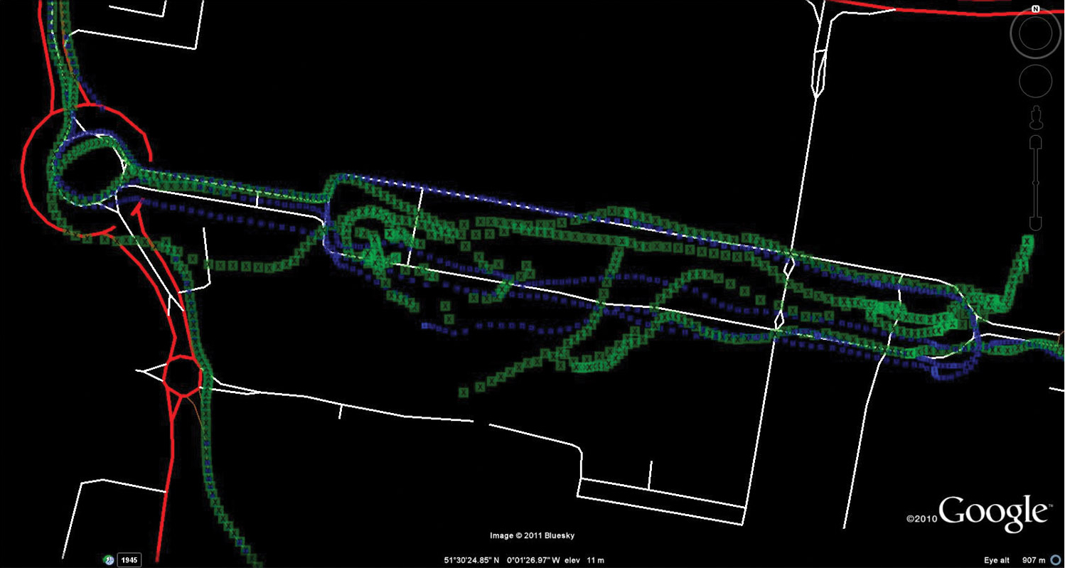
Figure 6 shows the same test data displayed on truth data taken from the ordnance survey vector map data of the roads.
Figure 6. GPS versus GNSS, London Canary Wharf, on vector truth (click to enlarge.)
The blue GNSS data is then extremely good, especially on the northern (eastbound) part of the loop (UK drives on the left, thus one-way loops are clockwise).
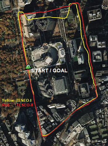
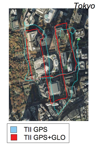
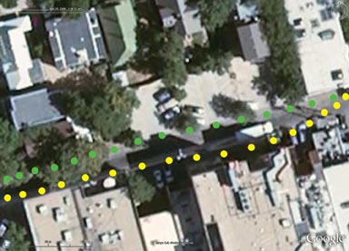
Further tests were carried out by ST offices around the world. Figure 7 shows a test in Tokyo, where yellow is the previous generation of chip with no GLONASS, red was Teseo-II with GPS plus GLONASS.
Figure 7. Teseo-I (GPS) versus Teseo-II (GNSS) in Tokyo test.
Again, here the scenario is not sufficiently challenging to hurt the availability even of GPS alone, but the accuracy is limited.
Figure 8 gives some explanation of the accuracy problems, by showing the DOP during the test. It can be seen that Teseo-II DOP was rarely above 2, but the GPS-only version was between 6 and 12 in the difficult northern part of the test, circled for illustration.
Figure 8. DOP during Tokyo tests (click to enlarge.)
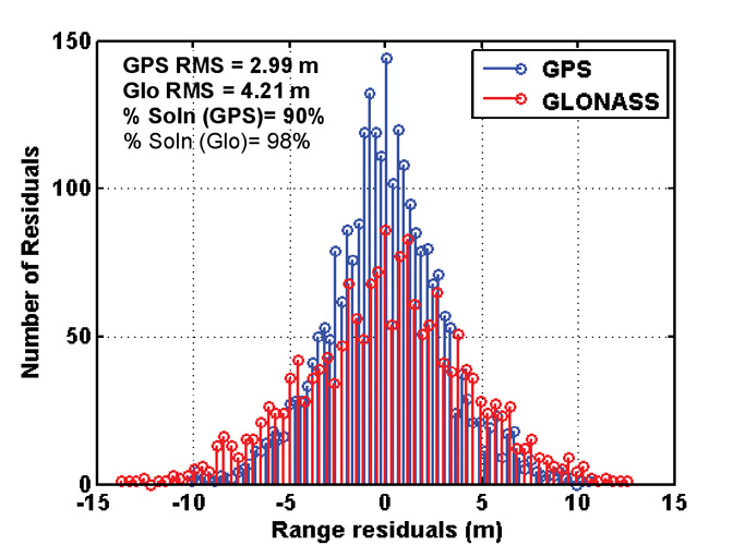
Further Tokyo tests were performed entering the narrower urban canyons in the same test area, shown in Figure 9. Blue is GPS only, red is GPS+GLONASS, and the major improvement is obvious.
Figure 9. GPS only (blue) versus GNSS (red), Tokyo.
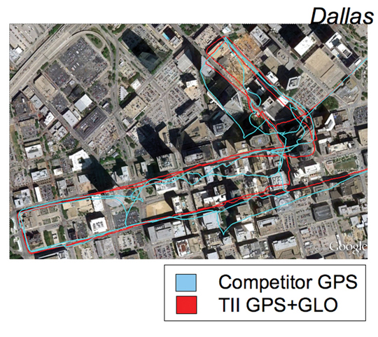
Figure 10 uses the same color scheme to illustrate tests in Dallas, this time with a competitor’s GPS receiver versus Teseo-II configured for GPS+GLONASS, again a huge benefit.
Figure 10. GPS only (blue, competitor) versus GNSS (red), Dallas.
Other Constellations
While Teseo-II hardware supports Galileo, there are no production Galileo satellites available yet (September 2011), so the units in the field do not have Galileo software loaded.
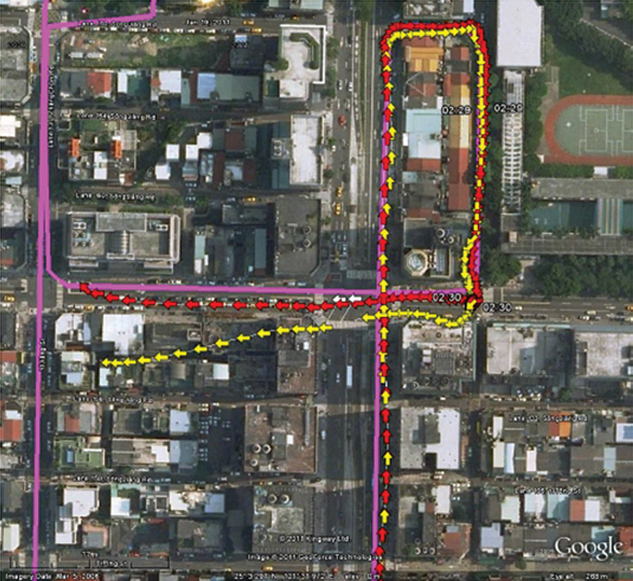
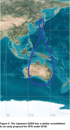
However, the Japanese QZSS system has one satellite available, transmitting legacy GPS-compatible signals, SBAS signals, and L1C BOC signals. Teseo-II can process the first two of these, and while SBAS is no benefit in the urban canyon as the problems of reflection and obstruction are local and unmonitored, the purpose of QZSS is to provide a very high-angle satellite, so that it is always available in urban canyons.
Figure 11 shows a test in Taipei (Taiwan) using GPS (yellow) versus GPS plus one QZSS satellite in red, with the truth data shown in purple.
Figure 11. GPS only (yellow) versus GPS+QZSS(1 sat, red), truth in purple, Taipei (click to enlarge.)
Further Work
The test environment will be extended to yield quantitative accuracy results for UK tests where we have the vector truth data for the roads.
The hardware flexibility will be extended to support Compass and GPS-III (L1-C) signals, in addition to Galileo already supported. Acquisition and tracking of these signals have already been demonstrated using pre-captured off-air samples.
In 2010, the Compass spec was not available. Thus the Teseo-II silicon design was oriented to maximum flexibility in terms of different code lengths, such as BOC or BPSK, so that by using software to configure the hardware DSP functions, the greatest chance of compatibility could be achieved.
The result was only a marginal success, in that the 1561 MHz frequency of the regional Compass system can only be supported using the flexibility of the voltage-controlled oscillator and PLL, meaning that it cannot be supported at the same time as other constellations. Additionally, the code rate on the regional system is also 2 M chips/second, which is not supported, so is approximated by using alternate chips, producing serious signal loss.
So the hooks for Compass are only useful for research and software development, either for a single-constellation system, or using a separate RF front end.
The worldwide Compass signal, which is on a GPS/Galileo signal format in both carrier frequency and in code length and rate, will be directly compatible, but is not expected to be fully available until 2020.
The city environment testing will be repeated as the Galileo constellation becomes available. With 32 channels, an 11/11/10 split (GPS/Galileo/GLONASS) may be used when all three constellations are full, but for the next few years 14/8/10 satisfies the all-in-view requirements.
Conclusions
The multi-constellation receiver can include GLONASS FDMA at minimal increased cost, and with its 32 channels tracking up to 22 satellites in a benign environment, even in the harshest city environment sufficient satellites are seen for 100 percent availability and acceptable accuracy. 10–16 satellites were generally seen in the urban canyon tests. The multiplicity of measurements allows RAIM and FDE algorithms to be far more effective in eliminating badly reflected signals, and also minimizes the geometric effects of remaining distortion on the signals retained.
Acknowledgments
ST GPS products, chipsets, and software, baseband and RF are developed by a distributed team in Bristol, UK (system R&D, software R&D); Milan, Italy (silicon implementation, algorithm modelling and verification); Naples, Italy (software implementation and validation); Catania, Sicily, Italy (Galileo software, RF design and production); and Noida, India (verification and FPGA). The contribution of all these teams to both product ranges is gratefully acknowledged.
Philip Mattos received a master’s degree in electronic engineering from Cambridge University, UK, a master’s in telecoms and computer science from Essex University, and an external Ph.D. for his GPS work from Bristol University. He was appointed a visiting professor at the University of Westminster. Since 1989 he has worked exclusively on GPS implementations and associated RF front ends, currently focusing on system-level integrations of GPS, on the Galileo system, and leading the STMicroelectronics team on L1C and Compass implementation, and the creation of generic hardware to handle future unknown systems.
By Pratibha B. Anantharamu, Daniele Borio, and Gérard Lachapelle
Spatial and temporal information of signals received from multiple antennas can be applied to mitigate the impact of new GPS and Galileo signals’ binary-offset sub-carrier, reducing multipath and interference effects.
New modernized GNSS such as GPS, Galileo, GLONASS, and Compass broadcast signals with enhanced correlation properties as compared to the first generation GPS signals. These new signals are characterized by different modulations that provide improved time resolution, resulting in more precise range measurements, along with the advantage of being more resilient to multipath and RF interference. One of these modulations is the binary-offset-carrier (BOC) modulation transmitted by Galileo and modernized GPS.
Despite the benefits of BOC modulation schemes, difficulties in tracking BOC signals can arise. The autocorrelation function (ACF) of BOC signals is multi-peaked, potentially leading to false peak-lock and ambiguous tracking. Intense research activities have produced different BOC tracking schemes that address the issue of multi-peaked BOC signal tracking. Additionally, new tracking schemes including space-time processing can be adopted to further improve the performance of existing algorithms.
Space-time equalization is a technique that utilizes spatial and temporal information of signals received from multiple antennas to compensate for the effects of multipath fading and co-channel interference. In the context of BOC signals, these kinds of techniques can be applied to mitigate the impact of the sub-carrier, which is responsible for a multi-peaked ACF, reducing multipath and interference effects. In temporal processing, traditional equalizers in time-domain are useful to compensate for signal distortions. But equalization becomes more challenging in the case of BOC signals, where the effect of both sub-carrier and multipath must be accounted for. On the other hand, by using spatial processing, it should be possible to extract the desired signal component from a set of received signals by electronically varying the antenna array directivity (beamforming).
The combination of an antenna array and a temporal equalizer results in better system performance. Hence the main objective of this research is to apply space-time processing techniques to BOC modulated signals received by an antenna array. The main intent is to enhance the signal quality, avoid ambiguous tracking and improve tracking performance under weak signal environments or in the presence of harsh multipath components.
The focus of previous antenna-array processing using GNSS signals was on enhancing GNSS signal quality and mitigating interference and/or multipath related issues. Unambiguous tracking was not considered. Here, we develop a space-time algorithm to mitigate ambiguous tracking of BOC signals along with improved signal quality. The main objective is to obtain an equalization technique that can operate on BOC signals to provide unambiguous BPSK-like correlation function capable of altering the antenna array beam pattern to improve the signal to interference plus noise ratio.
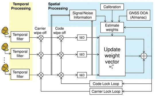
Space-time adaptive processing structure proposed for BOC signal tracking; the temporal filter provides signal with unambiguous ACF whereas the spatial filter provides enhanced performance with respect to multipath, interference, and noise.
Initially, temporal equalization based on the minimum mean square error (MMSE) technique is considered to obtain unambiguous ACF on individual antenna outputs. Spatial processing is then applied on the correlator outputs based on a modified minimum variance distortionless response (MVDR) approach. As part of spatial processing, online calibration of the real antenna array is performed which also provides signal and noise information for the computation of the beamforming weights. Finally, the signal resulting from temporal and spatial equalization is fed to a common code and carrier tracking loop for further processing.
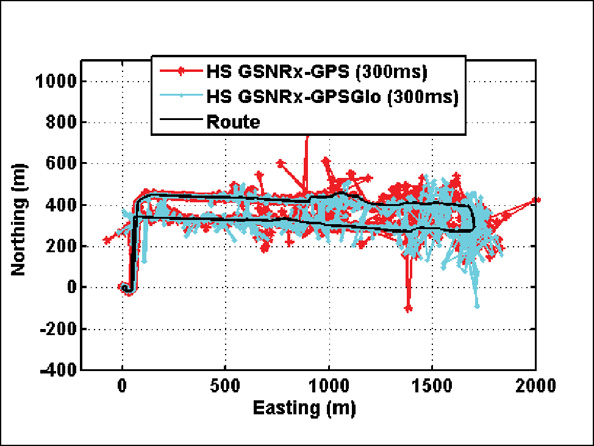
The effectiveness of the proposed technique is demonstrated by simulating different antenna array structures for BOC signals. Intermediate-frequency (IF) simulations have been performed and linear/planar array structures along with different signal to interference plus noise ratios have been considered. A modified version of The University of Calgary software receiver, GSNRx, has been used to simultaneously process multi-antenna data. Further tests have been performed using real data collected from Galileo test satellites, GIOVE-A and GIOVE-B, using an array structure comprising of two to four antennas. A 4-channel front-end designed in the PLAN group, and a National Instruments (NI) signal vector analyzer equipped with three PXI-5661 front-ends (NI 2006) have been used to collect data synchronously from several antennas. The data collected from the antennas were progressively attenuated for the analysis of the proposed algorithm in weak signal environments.
From the performed tests and analysis, it is observed that the proposed methodology provides unambiguous ACF. Spatial processing is able to efficiently estimate the calibration parameters and steer the antenna array beam towards the direction of arrival of the desired signal. Thus, the proposed methodology can be used for efficient space-time processing of new BOC modulated GNSS signals.
Signal and Systems Model
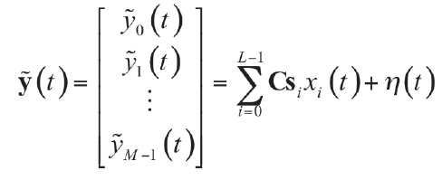
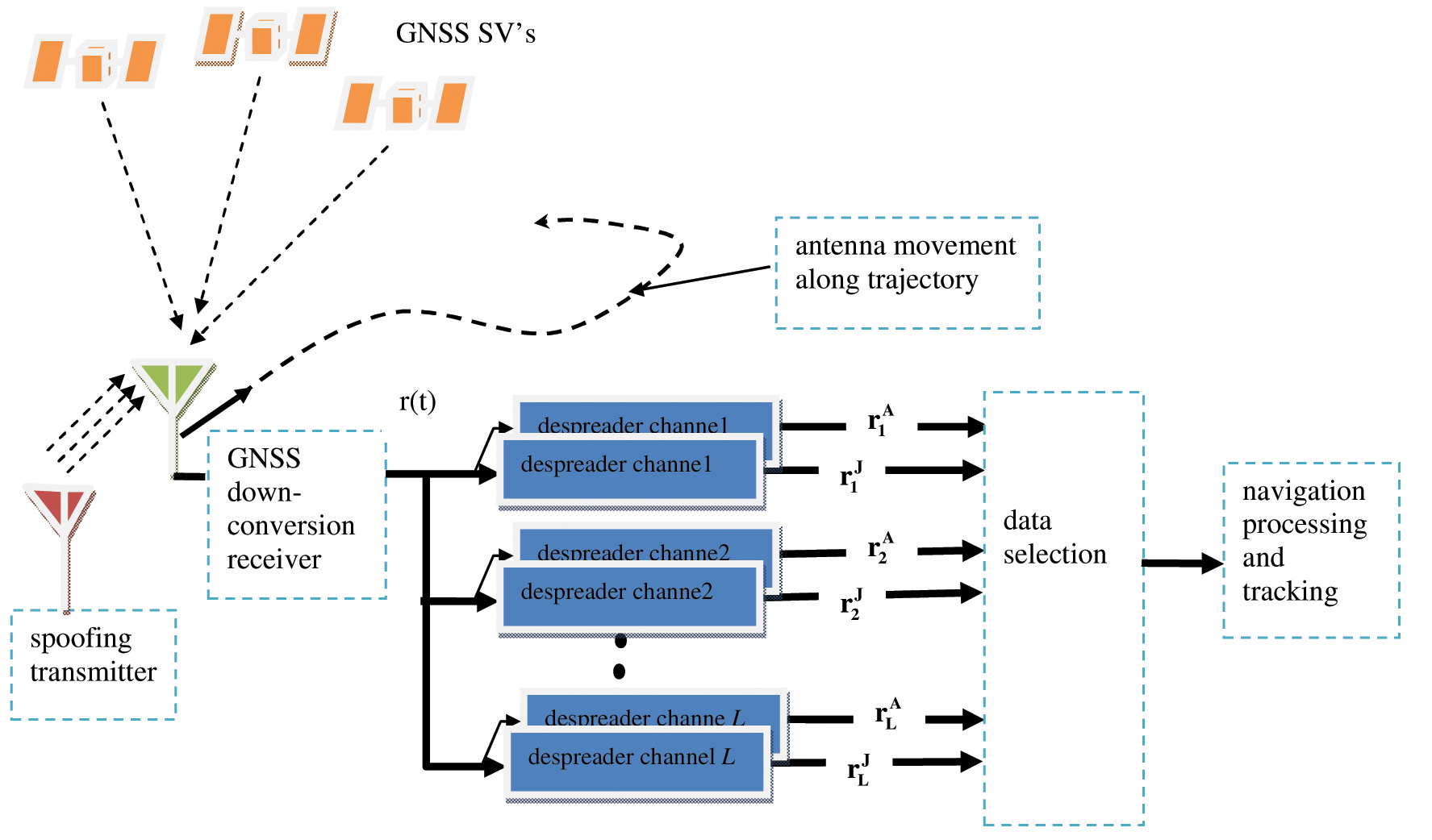
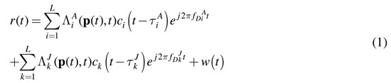
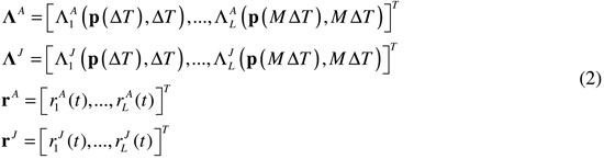
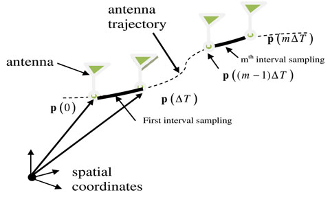
The complex baseband GNSS signal vector received at the input of an antenna array can be modeled as (1)
where
• M is the number of antenna elements;
• L is the number of satellites;
• C is a M × M calibration matrix capturing the effects of antenna gain/phase mismatch and mutual coupling;
• si = is the complex M × 1 steering vector relative to the signal from the ith satellite. si captures the phase offsets between signals from different antennas;
• is the noise plus interference vector observed by the M antennas.
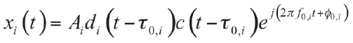
The ith useful signal component xi (t) can be modeled as (2)
where
• Ai is the received signal amplitude;
• di() models the navigation data bit;
• ci() is the ranging sequence used for spreading the transmitted data;
• τ0,i, f0,i and φ0,imodel the code delay, Doppler frequency and carrier phase introduced by the communication channel.
The index i is used to denote quantities relative to the ith satellite. The ranging code ci() is made up of several components including a primary spreading sequence, a secondary code and a sub-carrier.
For a BPSK modulated signal, the sub-carrier is a rectangular window of duration Tc. In the case of BOC modulated signals, the sub-carrier is generated as the sign of a sinusoidal carrier. The presence of this sub-carrier produces a multi-peaked autocorrelation function making the acquisition/tracking processes ambiguous.
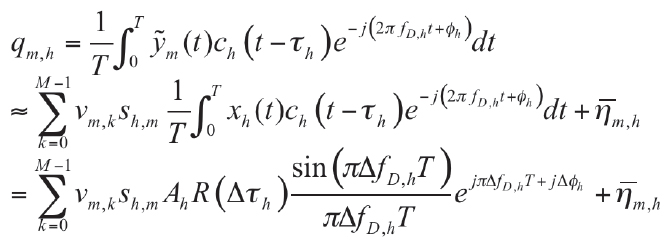
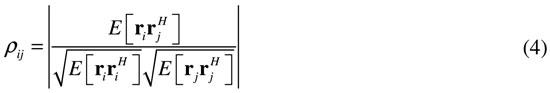
In order to extract signal parameters such as code delay and Doppler frequency of the ith useful signal xi(t), the incoming signal is correlated with a locally generated replica of the incoming code and carrier. This process is referred to as correlation where the carrier of the incoming signal is at first wiped off using a local complex carrier replica. The spreading code is also wiped off using a ranging code generator. The signal obtained after carrier and code removal is integrated and dumped over T seconds to provide correlator outputs. The correlator output for the hth satellite and mth antenna can be modeled as: (3)
where vm,kare the coefficients of the calibration matrix, C and R(Δτh) is the multi-peaked ACF. τh, fD,h and φh are the code delay, Doppler frequency and carrier phase estimated by the receiver and Δτh, ΔfD,h and Δφh are the residual delay, frequency, and phase errors. is the residual noise term obtained from the processing of η(t). Eq. (3) is the basic signal model that will be used for the development of a space-time technique suitable for unambiguous BOC tracking.
When BOC signals are considered, algorithms should be developed to reduce the impact of that include receiver noise, interference and multipath components, along with the mitigation of ambiguities in R(Δτh). Space-time processing techniques have the potential to fulfill those requirements.
Space-Time Processing
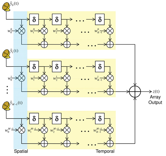
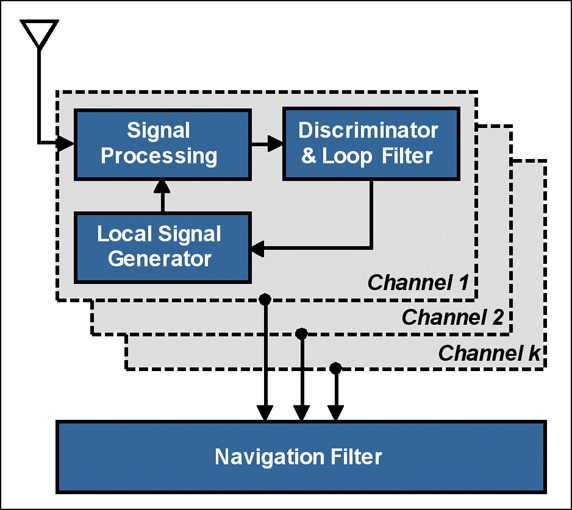
A simplified representation of a typical space-time processing structure is provided in Figure 1. Each antenna element is followed by K taps with δ denoting the time delay between successive taps forming the temporal filter. The combination of several antennas forms the spatial filter. wmk are the space-time weights with 0 ≤ k ≤ K and 0 ≤ m ≤ M. k is the temporal index and m is the antenna index.
Figure 1. Block diagram of space-time processing.
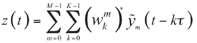
The array output after applying the space-time filter can be expressed as (4)
where (wmk)* denotes complex conjugate. The spatial-only filter can be realized by setting K=1 and a temporal only filter is obtained when M=1. The weights are updated depending on the signal/channel characteristics subject to user-defined constraints using different adaptive techniques. This kind of processing is often referred to as Space-Time Adaptive Processing (STAP). The success of STAP techniques has been well demonstrated in radar, airborne and mobile communication systems. This has led to the application of STAP techniques in the field of GNSS signal processing. Several STAP techniques have been developed for improving the performance of GNSS signal processing. These techniques exploit the advantages of STAP to minimize the effect of multipath and interference along with improving the overall signal quality.
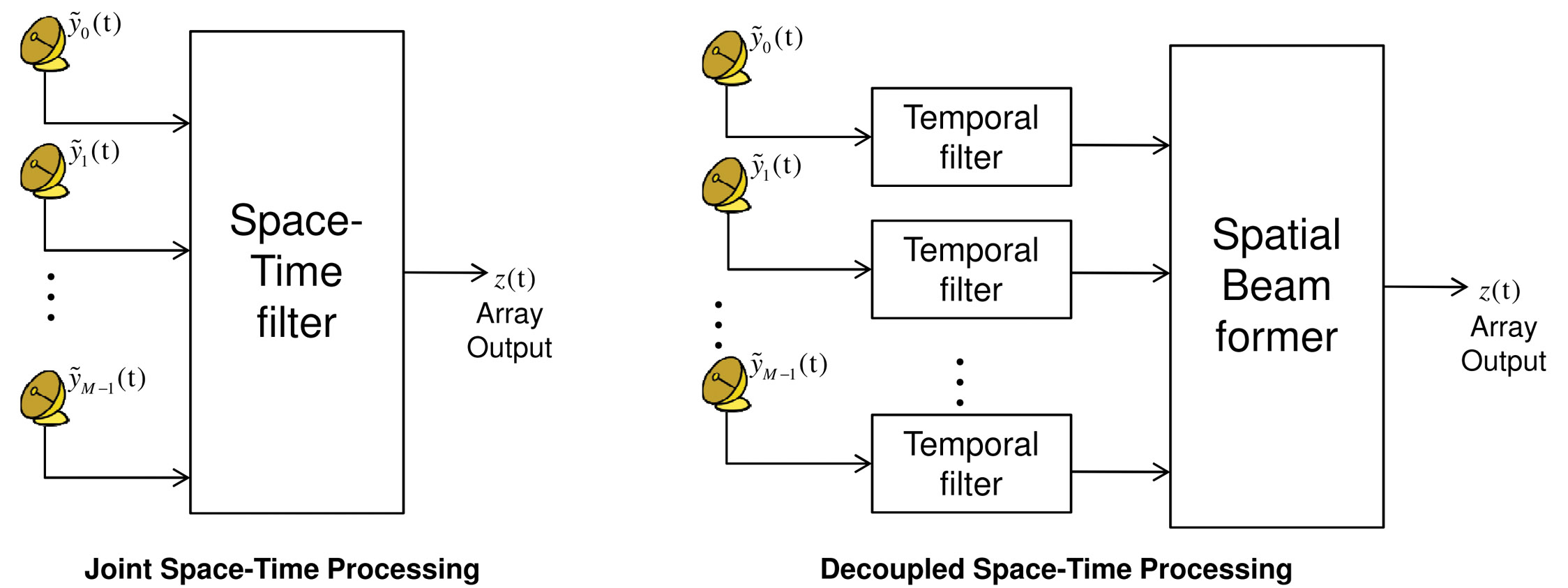
Space-time processing algorithms can be broadly classified into two categories: decoupled and joint space-time processing. The joint space-time approach exploits both spatial and temporal characteristics of the incoming signal in a single space-time filter while the decoupled approach involves several temporal equalizers and a spatial beamformer that are realized in two separate stages (Figure 2).
Figure 2. Representation of two different space-time processing techniques
When considering the decoupled approach for GNSS signals, temporal filters can be applied on the data from the different antennas whereas the spatial filter can be applied at two different stages, namely pre-correlation or post-correlation. In the pre-correlation stage, spatial weights are applied on the incoming signal after carrier wipe-off while in the post-correlation stage, spatial weights are applied after the Integrate & Dump (I&D) block on the correlator outputs. In pre-correlation processing, the update rate of the weight vector is in the order of MHz (same as the sampling frequency) whereas the post-correlation processing has the advantage of lower update rates in the order of kHz (I&D frequency). In the pre-correlation case, the interference and noise components prevail significantly in the spatial correlation matrix and would result in efficient interference mitigation and noise reduction. But the information on direct and reflected signals are unavailable since the GNSS signals are well below the noise level. This information can be extracted using post-correlation processing.
In the context of new GNSS signals, efforts to utilize multi-antenna array to enhance signal quality along with interference and multipath mitigation have been documented using both joint and decoupled approaches where the problem of ambiguous signal tracking was not considered.
In our research, we considered the decoupled space-time processing structure. Temporal processing is applied at each antenna output and spatial processing is applied at the post-correlation stage. Temporal processing based on MMSE equalization and spatial processing based on the adaptive MVDR beamformer are considered.
Methodology
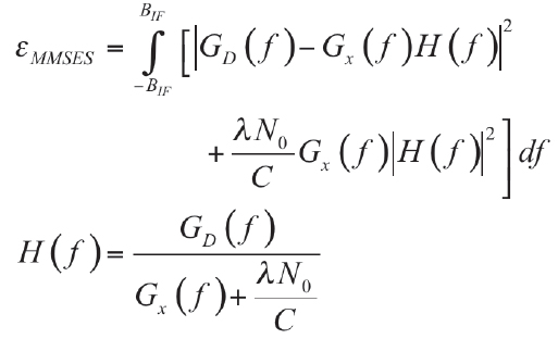
The opening figure shows the proposed STAP architecture for BOC signal tracking. In this approach, the incoming BOC signals are at first processed using a temporal equalizer that produces a signal with a BPSK-like spectrum. The filtered spectra from several antennas are then combined using a spatial beamformer that produces maximum gain at the desired signal direction of arrival. The beamformed signal is then fed to the code and carrier lock loops for further processing. The transfer function of the temporal filter is obtained by minimizing the error: (5)
where H(f) is the transfer function of the temporal filter that minimizes the MSE, εMMSES, between the desired spectrum, GD(f), and filtered spectrum, Gx(f)H(f). The spectrum of the incoming BOC signal is denoted by Gx(f). λ is a weighting factor determining the impact of noise with respect to that of an ambiguous correlation function. N0 is the noise power spectral density and C the carrier power. The desired spectrum is considered to be a BPSK spectrum. Since this type of processing minimizes the MSE, it is denoted MMSE Shaping (MMSES).
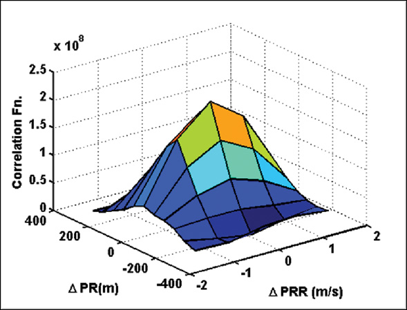
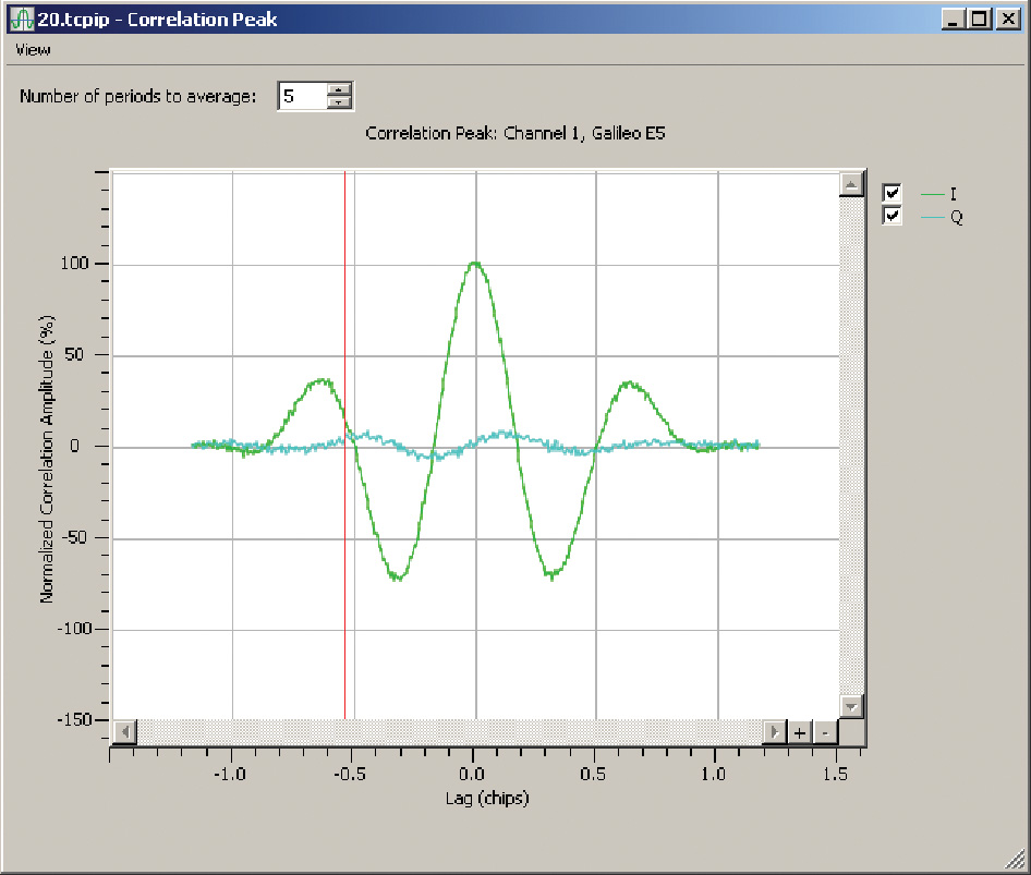
Figure 3 shows a sample plot of the ACF obtained after applying MMSES on live Galileo BOCs(1,1) signals collected from the GIOVE-B satellite. The input C/N0 was equal to 40 dB-Hz and the ACF was averaged over 1 second of data. It can be observed
that the multi-peaked ACF was successfully modified by MMSES to produce a BPSK-like ACF without secondary peaks. Also narrow ACF were obtained by modifying the filter design for improved multipath mitigation. Thus using temporal processing, the antenna array data are devoid of ambiguity due to the presence of the sub-carrier.
After temporal equalization, the spatial weights are computed and updated based on the following information:
The signal and noise covariance matrix obtained from the correlator outputs;
Calibration parameters estimated to minimize the effect of mutual coupling and antenna gain/phase mismatch;
Satellite data decoded from the ephemeris/almanac containing information on the GNSS signal DoA.
The weights are updated using the iterative approach for the MVDR beamformer to maximize the signal quality according to the following steps:
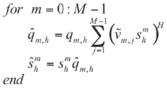
Step 1: Update the estimate of the steering vector for the hthsatellite using the calibration parameters as: (6)
Here vi,j represents the estimated calibration parameters using the correlator outputs given by Eq. (3) and shm is the element of the steering vector computed using the satellite ephemeris/almanac data.
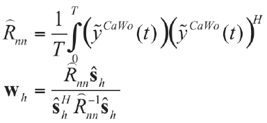
Step 2: Update the weight vector (the temporal index, k, is removed for ease of notation) using the new estimate of the covariance matrix and steering vector as (7)
where is the input signal after carrier wipe-off.
Repeat Steps 1 and 2 until the weights converge. Finally compute the correlator output to drive the code and carrier tracking loop according to Equation (4).
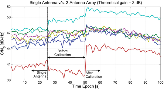
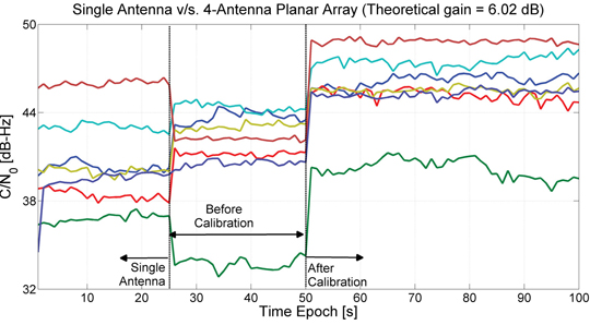
The C/N0 gain obtained after performing calibration and beamforming on a two-antenna linear array and four-antenna planar array data collected using the four channel front-end is provided in Figure 4 and Figure 5. The C/N0 plots are characterized by three regions:
Single Antenna that provides C/N0 estimates obtained using q0,h alone;
BeforeCalibration that provides C/N0 estimates obtained by compensating only the effects of the steering vector, si, before combining the correlator outputs from all antennas;
AfterCalibration that provides C/N0 estimates obtained by compensating the effects of both steering vector, si and calibration matrix, C, before combining correlator outputs from all antennas.
After calibration, beamforming provides approximately a C/N0 gain equal to the theoretical one on most of the satellites whereas before calibration, the gain is minimal and, in some cases, negative with respect to the single antenna case. These results support the effectiveness of the adopted calibration algorithm and the proposed methodology that enables efficient beamforming.
Figure 4. C/N0 estimates obtained after performing calibration and beamforming on linear array data.Figure 5. C/N0 estimates obtained after performing calibration and beamforming on the planar array data.
Results and Analysis
IF simulated BOCs(1,1) signals for a 4-element planar array with array spacing equal to half the wavelength of the incoming signal has been considered to analyze the proposed algorithm. The input signal was characterized by a C/N0 equal to 42 dB-Hz at an angle of arrival of 20° elevation and 315° azimuth angle.
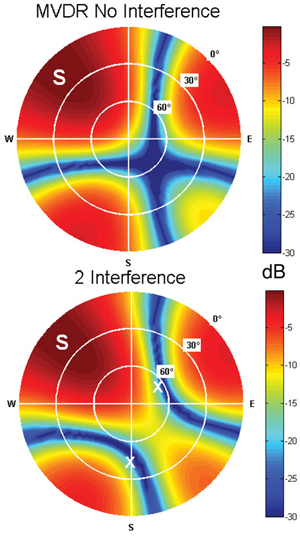
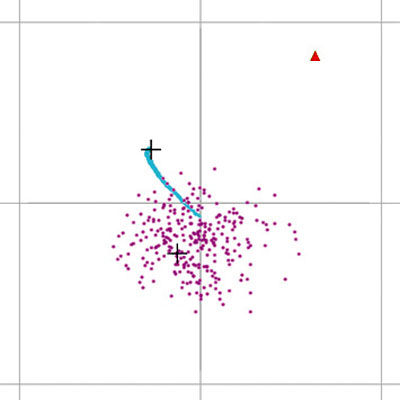
A sample plot of the antenna array pattern using the spatial beamformer is shown in Figure 6. In the upper part of Figure 6, the ideal case in the absence of interference was considered. The algorithm is able to place a maximum of the array factor in correspondence of the signal DoA.
Figure 6. Antenna array pattern for a 4-element planar array computed using a MVDR beamformer in the presence of two interference sources.
In the bottom part, results in the presence of interference are shown. Two interference signals were introduced at 60 and 45 degree elevation angles. It can be clearly observed that, in the presence of interference, the MVDR beamformer successfully adapted the array beam pattern to place nulls in the interference DoA.
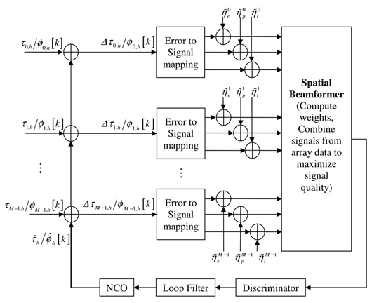
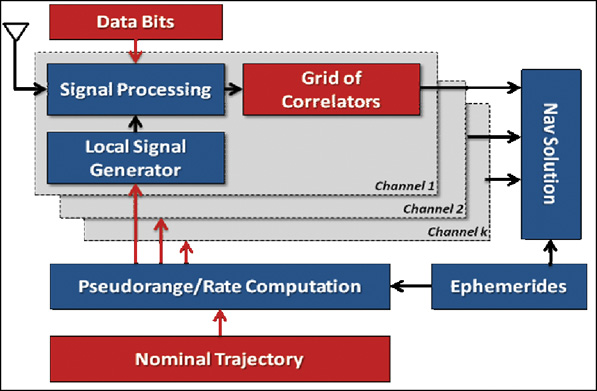
In order to further test the tracking capabilities of the full system, semi-analytic simulations were performed for the analysis of digital tracking loops. The simulation scheme is shown in Figure 7 and consists of M antenna elements. Each antenna input for the hth satellite is defined by a code delay (τm,h) and a carrier phase value (φm,h) for DLL and PLL analysis. φm,h captures the effect of mutual coupling, antenna phase mismatch and phase effects due to different antenna hardware paths. To analyze the post-correlation processing structure, each antenna input is processed independently to obtain the error signal, Δτm,h / Δφm,h as where are the current delay/phase estimates.
Figure 7. Semi-analytic simulation model for a multi-antenna system comprising M antennas with a spatial beamformer.
Each error signal is then used to obtain the signal components that are added along with the independent noise components, . The combined signal and noise components from all antenna elements are fed to the spatial beamformer to produce a single output according to the algorithm described in the Methodology section. Finally, the beamformer output is passed through the loop discriminator, filter and NCO to provide a new estimate . The Error to Signal mapping block and the noise generation process accounts for the impact of temporal filtering.
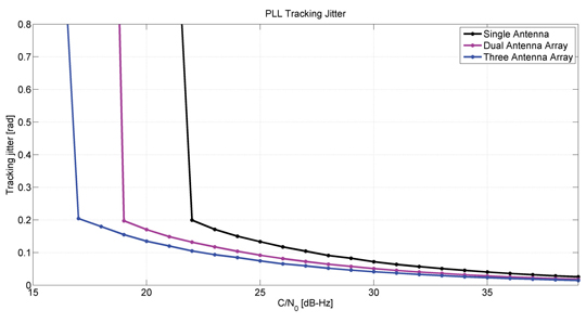
Figure 8 shows sample tracking jitter plots for a PLL with a single, dual and three-antenna array system obtained using the structure described above.
Figure 8. Phase-tracking jitter obtained for single, dual and three-antenna linear array as a function of the input C/N0 for a Costas discriminator (20 milliseconds coherent integration and 5-Hz bandwidth).
The number of simulation runs considered was 50000 with a coherent integration time of 20 ms and a PLL bandwidth equal to 5 Hz. As expected the tracking jitter improves when the number of antenna elements is increased along with improved tracking sensitivity. As expected, the C/N0 values at which loss of lock occurs for a three antenna system is reduced with respect to the single antenna system, showing its superiority.
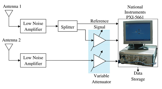
Real data analysis. Figure 9 shows the experimental setup considered for analysis of the proposed combined space-time algorithm. Two antennas spaced 8.48 centimeters apart were used to form a 2-element linear antenna array structure. The NI front-end was employed for the data collection process to synchronously collect data from the two-antenna system.
Data on both channels were progressively attenuated by 1 dB every 10 seconds to simulate a weak signal environment until an attenuation of 20 dB was reached. When this level of attenuation was reached, the data were attenuated by 1 dB every 20 seconds to allow for longer processing under weak signal conditions. In this way, data on both antennas were attenuated simultaneously. Data from Antenna 1 were passed through a splitter, as shown in Figure 9, before being attenuated in order to collect signals used to produce reference code delay and carrier Doppler frequencies.
Figure 9. Experimental setup with signals collected using two antennas spaced 8.48 centimeters apart.
BOCs(1,1) signals collected using Figure 9 were tracked using the temporal and spatial processing technique described in the opening figure. The C/N0 results obtained using single and two antennas are provided in Figure 10. In the single antenna case, only temporal processing was used. In this case, the loop was able to track signals for an approximate C/N0 of 19 dB-Hz. Using the space-time processing, the dual antenna system was able to track for nearly 40 seconds longer than the single antenna case, thus providing around 2 dB improvement in tracking sensitivity.
Figure 10. C/N0 estimates obtained using a single antenna, temporal only processing and a dual-antenna array system using space-time processing.
Conclusions
A combined space-time technique for the processing of new GNSS signals including a temporal filter at the output of each antenna, a calibration algorithm and a spatial beamformer has been developed. The proposed methodology has been tested with simulations and real data. It was observed that the proposed methodology was able to provide unambiguous tracking after applying the temporal filter and enhance the signal quality after applying a spatial beamformer. The effectiveness of the proposed algorithm to provide maximum signal gain in the presence of several interference sources was shown using simulated data. C/N0 analysis for real data collected using a dual antenna array showed the effectiveness of combined space-time processing in attenuated signal environments providing a 2 dB improvement in tracking sensitivity.
Pratibha B. Anantharamu received her doctoral degree from Department of Geomatics Engineering, University of Calgary, Canada. She is a senior systems engineer at Accord Software & Systems Pvt. Ltd., India.
Daniele Borio received a doctoral degree in electrical engineering from Politecnico di Torino. He is a post-doctoral fellow at the Joint Research Centre of the European Commission.
Gérard Lachapelle holds a Canada Research Chair in Wireless Location in the Department of Geomatics Engineering, University of Calgary, where he heads the Position, Location, and Navigation (PLAN) Group.
By Jenna R. Tong, Robert J. Watson, and Cathryn N. Mitchell, University of Bath
Using signal-to-noise measurements from a single commercial-grade L1 GPS receiver, it is possible to detect interference or jamming that is above the thermal noise floor and below a power that causes loss of position.
Interference, intentional or unintentional, is an acknowledged vulnerability of GPS systems. Many of the potential sources of interference are unintentional: interference can caused by harmonics of out-of-band signals, electronic noise, or malfunctioning equipment. The effect, however, is the same independent of intent.
The presence of high-power interference which causes continual denial of service is fairly easy to detect, but lower power interference may still degrade performance, for example by causing loss of lock on some satellites, thus increasing position dilution of precision, although the receiver continues to output a position. Short periods of denial of service caused by intermittent high-power interference may not be immediately detected depending on the timing and ability of the system in use to deal with temporary loss of signal.
Therefore, to fully characterize an antenna environment requires a 24/7 system, whether the purpose is to determine whether a location is suitable prior to installation, to identify whether problems at an existing site are due to interference, or to provide warnings of the presence of interference on a continuous basis. In particular, information on timing — for example finding a time of day or day of the week when interference is regularly seen — may assist in determining the source of the interference.
This research forms part of the GNSS Availability Accuracy Reliability anD Integrity Assessment for timing and Navigation (GAARDIAN) project, which provides a mesh of sensors to monitor the integrity, reliability, continuity, and accuracy of the locally received GPS (or other GNSS) and eLoran signals continuously and to detect anomalous conditions such as local interference, differentiating between possible sources of errors such as interference, multipath, satellite errors, or space weather.
Here we look at using the signal-to-noise ratio (SNR) values from a single-frequency GPS receiver to detect interference. There are two stages to the algorithm: determining the local environment of the antenna in terms of multipath and interference, and identifying and recording potential interference events.
Since this method uses values output from a GPS receiver, characterizing the response to interference of the receiver used in the probe is necessary, to indicate what level interference can be detected with the system, as well as ensuring that false positives are not produced, and the effects of interference can be separated from those of multipath and scintillation, which can also cause decreases in SNR.
We used a commercial, single-frequency receiver, recording this data from NMEA messags for analysis:
SNR, in dB, reported as an integer
elevation, in degrees, reported as an integer
azimuth, in degrees, reported as an integer
carrier lock time, in seconds.
Algorithm. To determine the presence of interference, the normal state of the receiver must first be calculated. Initially it is assumed the receiver is fixed with an unchanging multipath environment. SNR and elevation values from all satellites are accumulated for several hours. To reduce influence of the unknown multipath environment, values from satellites below 10 degrees elevation and from those where the carrier lock time is less than four minutes are removed from the data set.
A polynomial fit between elevation and SNR is then calculated from the remaining data. A second- or third-degree polynomial generally fits the high-elevation data with deviations from the profile at low elevations being primarily due to multipath where interference is not present.
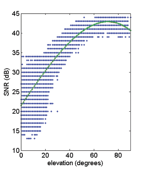
The standard deviation of SNR at each elevation is then calculated. The combination of the polynomial and these values of standard deviation characterize the normal environment of the receiver, for the case where interference is not present in the data gathered (Figure 1).
Figure 1. Raw SNR data against elevation, for all satellites in view over a period of 12 hours (blue), and a polynomial fitting to the same data (green).
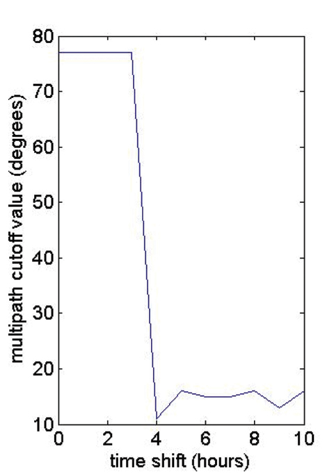
To confirm that the threshold values returned by the first stage of the algorithm are valid, a value is calculated for the elevation where the SNR value drops below the polynomial curve by the greatest amount.
If interference is not present, this is normally found at the point where multipath begins to influence the incoming signal and can be considered as a rough multipath cutoff, used to remove signals that may be influenced by multipath from later stages of the analysis.
Assuming a well-sited antenna, a value greater than 25 degrees for this value indicates the possible presence of interference in the data used to calculate the polynomial. In cases where this value is high, the data in question would be rejected, and optionally a user may be warned that there may be pre-existing interference. If the antenna-receiver combination has been previously calibrated in a known good environment, it would be also possible to identify interference based on the difference in polynomial and standard deviation values between that environment and the location being tested.
Figure 2 shows the value of this multipath cutoff (in degrees) for a set of data where interference was known to be present initially, against the start time for the data used to calculate the polynomial and multipath cutoff values, by number of hours from the start of the file.
Once the mask is developed, a threshold value can be set to be n standard deviations below the polynomial, and events are detected by the combination of:
At least four satellites with elevations above the multipath cutoff which are below the threshold value or which were above the multipath cutoff previous to losing lock.
This status is continuous for more than a set time t.
Requiring multiple satellites limits the effects of other influences on SNR such as multipath; requiring an extended time period removes very short-term fluctuations.
The number of false positives and the power of interference required to cause an alarm then depends primarily on the value of the threshold factor n, and on the time period t, which here we kept at a constant of 30 seconds.
Testing
To avoid radiating interference, we constructed an RF network to facilitate injection of jamming signals into the GPS signal path. The GPS signal from a roof-mounted choke-ring antenna was passed through an amplifier and attenuator chain to provide 0 dB forward gain, but around 40 dB reverse isolation. An additional stepped attenuator (0–40 dB in 1 dB steps) was also included. The buffered signal from the antenna was then combined with the output of a vector signal generator used to provide the jamming signal.
The combined signal was then fed into the GPS receiver via a DC-block to remove the antenna bias voltage. The signal generator is capable of producing a wide variety of jamming including matched spectrum wideband noise, CW, and pulsed signals. The adjustment of both the signal generator output power and the signal attenuator a
llow the replication of a variety of signal-to-noise and jammer-to-noise scenarios.
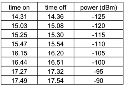
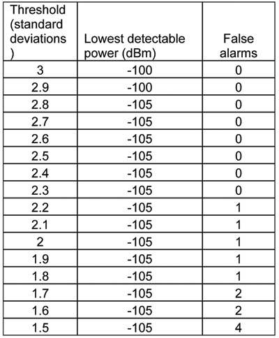
With the receiver locked onto a stable position, CW signals at L1 frequency were introduced into the receiver at levels from –125 dBm to –90 dBm in steps of 5 dBm, with at least 15 minutes of buffer time for the receiver to recover between each step (Table 1). Data was logged at 1 Hz throughout. We collected 20 hours of data, to calculate threshold values from data with no known interference.
Table 1.
Results
Twelve hours of data from a period where no known interference was present was used to form the SNR mask, and events longer than 30 seconds were looked for using various values of n for the threshold across all 20 hours of data. A false alarm was considered to be any event where interference was detected while the signal generator was off. Table 2 summarizes the response for different threshold levels.
Table 2.
In this test, CW interference of –100 dBm was required before the number of satellites with carrier lock dropped below four even for a single epoch, and –90 dBm was required to cause a sustained loss of lock, but jamming of –105 dBm was still detectable by this system with no false positives returned.
Decreasing the threshold began to produce false positives without detecting the smaller interference signals. This is not surprising as the thermal noise floor, assuming 2 MHz bandwidth, is about –110 dBm.
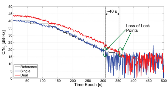
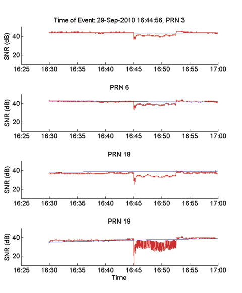
In the raw data from the detected events, a sharp dip in SNR is often seen at the beginning of an event, followed by recovery as the receiver compensates. In this particular case, where the aim is to detect the interference, this could lead to interference going undetected if the initial sharp dip was underneath the time threshold (30 seconds) and the recovery took the SNR of some of the satellites above the SNR threshold (Figure 3).
Figure 3. Value of polynomial mask (blue) and actual SNR (red) as recorded for four satellites during the period around the injection of the -100 dBm CW signal, showing initial dip and partial recovery.
Conclusion
Using only SNR values from a low-cost L1 GPS receiver, it is possible to detect CW interference which is above the thermal noise floor and below a power that causes loss of position. Different types of interference are expected to produce a different response, and unintentional interference is likely to be broadband or not directly centered on L1. The antenna used may also have a strong effect. These factors have not been examined here, although in practice the algorithm has run in multiple locations with different antennas, both direct and via splitters.
Regardless of the precise type of interference, the system would be expected to detect any interfering signal which impacts the SNR of the receiver, and to do so even if the signal strength was below a level which caused denial of service in that area.
The results are specific to the receiver used and its response to interference, although the algorithm would be capable of using data from any receiver that provided SNR values. Ideally the system used for measurement would have little or no built-in interference rejection.
Although this data was collected and then examined after the fact for signs of interference, the system works in precisely the same way in real time. Further trials will test the algorithm’s performance in real time and with different jamming scenarios, and compare results from multiple receivers in a single location and the performance of the algorithm with different antennas.
Acknowledgments
This work was funded by the Engineering and Physical Sciences Research Council and the Technology Strategy Board.
Jenna R. Tong is a postdoctoral researcher in electronic and electrical engineering at the University of Bath. Her Ph.D. in electron tomography is from the University of Cambridge.
Robert J. Watson received a Ph.D. degree in electronic engineering from the University of Essex, and is senior lecturer in electronic and electrical engineering at the University of Bath.
Cathryn N. Mitchell is a professor of engineering at the University of Bath and the Director of Invert Centre for Imaging Science. She received a Ph.D. from the University of Wales Aberystwyth.
By Thomas A. Stansell, Kenneth W. Hudnut, and Richard G. Keegan
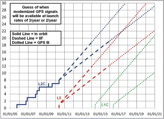
The new GPS L1C signal will be broadcast by the Block III satellites, with first launches as early as 2014. L1C innovations significantly enhance PNT performance as well as interoperability with other GNSS signals. The authors describe the benefits of its new features and how best to make use of each one.
A highly evolved racehorse of a signal with outstanding technical performance, L1C was designed to significantly improve autonomous navigation, and to be interoperable with L1 signals from other GNSS providers. Its structure evolved from the earliest GPS signals: it shares with the C/A signal the L1 center frequency of 1575.42 MHz, coherence between the carrier frequency, the code clock rates, and the data rate, and the provision of a navigation data message.
L1C inherited significant improvements from subsequent developments, specifically WAAS, L5, and L2C. WAAS was the first GPS-related signal to use forward error correction (FEC) for its data. L5 was the first open signal design to use longer spreading codes (10,230 chips), to have separate data and data-less (pilot carrier) signal components, to employ an improved navigation message structure (CNAV), and to employ overlay codes to achieve a longer equivalent code length, improve correlation performance, and eliminate the need for bit synchronization. The L2C signal adopted most of these improvements but, instead of an overlay, substituted a much longer pilot carrier spreading code, not only to optimize correlation performance but also to decrease the number of time ambiguities after tracking the spreading codes.
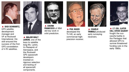
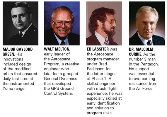
The L1C signal design is amazing, not only because of its highly evolved and outstanding technical performance but also because a committee designed this racehorse of a signal rather than it becoming a camel. Table 1 lists key members of the L1C technical committee in alphabetical order. The list has two groups, technical contributors and government chairpersons. When each new signal aspect is introduced, the key contributor or contributors from this list will be identified.
Table 1. Key L1C contributors.
L1C is intended to be interoperable with L1 signals from other GNSS providers. To identify its signal type, we note that Galileo officials have identified three types of services, “open”, “commercial”, and “publicly regulated”. An open service is freely available to all users. A commercial service is limited to users who pay a fee to access the signal, which otherwise is denied by encryption. A publicly regulated service (PRS) also is encrypted but intended only for public safety applications. GPS is adopting the open service definition but will continue to distinguish encrypted signals as “military” because there are no encrypted commercial GPS services. L1C will be a new GPS open service signal, joining L1 C/A, L2C, and L5.
Although the term “civil signal” often is used, there can be confusion about its meaning. Within the U.S. government it is common to use the word “civil” to mean civil government agencies, e.g., the Department of Transportation (DOT). However, it’s clear the GPS C/A, L2C, L5, and L1C signals are “open” and intended for use by anyone. Therefore, we will use the term “civilian” or “open” in order not to imply that any of these signals is restricted in its use.
L1C Signal Development
The L1C signal structure has evolved from the earliest GPS signals first launched in 1978. It shares with the C/A signal the L1 center frequency of 1575.42 MHz, coherence between the carrier frequency, the code clock rates, and the data rate, and the provision of a navigation data message. Significant improvements have been inherited from subsequent developments, specifically WAAS, L5, and L2C. For GPS or GPS-related signals, WAAS was the first to use forward error correction (FEC) for its data. L5 was the first open signal design to use longer spreading codes (10,230 chips), to have separate data and data-less (pilot carrier) signal components, to employ an improved navigation message structure (CNAV), and to employ overlay codes to achieve a longer equivalent code length, improve correlation performance, and eliminate the need for bit synchronization. The L2C signal adopted most of these improvements but, instead of an overlay, substituted a much longer pilot carrier spreading code, not only to optimize correlation performance but also to decrease the number of time ambiguities after tracking the spreading codes, i.e., extend the duration of GPS time ambiguity from 1 ms after tracking the C/A code and 20 ms after tracking the L5Q code to 1.5 sec for L2C.
Before giving details of the L1C signal in which we identify the primary contributor(s) for each innovation, it’s appropriate to recognize the special contributions of two members of the L1C technical team.
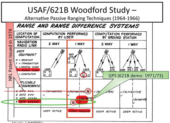
The first is Dr. Charles R. (Charlie) Cahn. Cahn has been a major contributor to GPS since before GPS was conceived. In particular, he was a key contributor to the Air Force 621B program which anticipated GPS. (He, Dr. James J. (Jim) Spilker, Dr. Robert Gold, and Mr. Burt Glazer deserve most of the credit for developing the original GPS C/A and P code signal structures, other than the NAV message.) Cahn discussed the merits of having a separate data-less or pilot channel in a 621B report [1], with Stansell he again recommended this for GPS in a 1975 Spartan Study Report, and finally the idea was adopted by the RTCA for L5 in accordance with recommendations from Cahn, Stansell, and Keegan. Also, Cahn was the first to recommend an overlay code on the L5 data signal to eliminate the need for the always problematic bit synchronization process. In a step toward L1C, Cahn was a primary contributor to the L2C design. In particular, he designed the code generators, including the 1.5 sec pilot code, and the chip by chip multiplexing technique which permitted two signal components in one bi-phase signal. In addition to consulting for The Aerospace Corporation and several commercial GPS companies, Cahn recently invented a more effective method to combine multiple signals on one carrier, called Phase-Optimized Constant-Envelope Transmission (POCET) modulation [2]. It is expected to be used on later versions of GPS III satellites to improve transmitter efficiency.
The second special recognition is for Dr. John Betz. Betz has played a very significant role for more than a decade in helping define the military M-code, in working with international partners to define and negotiate compatibility and interoperability signal parameters, in helping negotiate a significant part of the 2004 EU/US agreement, and in evaluating and supporting a wide variety of GPS programs and initiatives. Betz was a vital contributor to the overall L1C design through interaction with other team members, development of ways to compare alternatives, suggesting use of new signal processing concepts, and bringing experts from MITRE who performed significant analyses and developed key signal components.
Table 2 lists, in order of the authors’ judgment of value to user communities, the most important new characteristics of the L1C signal. The list also shows the primary contributor(s) for each characteristic.
Table 2. L1C Innovations in order of judged value.
Improvements made to the previously modernized civilian GPS signals, L5 and L2C, were a starting point for the L1C design. These included: having a pilot carrier; longer spreading codes (10,230 chips minimum); overlay or long pilot codes to eliminate the need for bit synchronization, to improve correlation properties, and to decrease the number of time ambiguities aft
er locking to the spreading codes; use of FEC to improve data demodulation performance and provide bit synchronization; and the flexible and higher precision CNAV message. The following paragraphs describe the additional improvements incorporated in L1C.
A key issue was whether additional signals could be added to the L1 carrier without negatively impacting legacy signals. Several combining methods were considered, and it was determined that, with the right combining technique, L1C could be added without detriment. Use of POCET, subsequently invented by Cahn, will further enhance this capability.
An “industry standard” rate ½ constraint length 7 convolutional coding method had been adopted for forward error correction (FEC) on WAAS, L2C, and L5 signals. However, the team agreed it was appropriate to consider other possibilities. Betz arranged for Ma to address the team on at least two occasions, providing a good tutorial on other advanced FEC methods which would allow message demodulation at even lower signal-to-noise ratios.
While the FEC options were being considered, another breakthrough occurred. Since at least 1999 Stansell had encouraged development of a way to take better advantage of GPS message redundancy. Rising to this challenge, Kovach proposed a modification of the CNAV message structure that he and Art Dorsey (Lockheed-Martin) had developed for L5 and L2C. The modified message, called CNAV-2, is equally flexible, equally precise, but more efficient, allows faster time to first fix (TTFF), and permits message demodulation at signals as weak as the carrier can be tracked. This final attribute requires FEC encoding of entire message blocks (sub-frames) rather than having the continuous process used for L2C and L5. As a result, when signal levels are very weak, bit symbols from two or more messages can be combined to improve the energy available per symbol, i.e., the L1C data demodulation threshold can be improved by combining symbols from two or more messages.
As a result of the message format improvements and performance evaluations by Shane, the team settled on the Low Density Parity Check (LDPC) FEC block encoding technique. This technique is as effective as turbo codes but without intellectual property constraints. Software developed by Shane was used by Sklar and Wang to define the specific L1C implementation, with performance simulation help from Kasemsri and Zapanta.
The most important new attribute of L1C resulted from a proposal by Betz to take advantage of the improved FEC and message redundancy attributes of L1C by having two separate data messages. Half the total signal power would be in the pilot carrier and the other half would be split evenly between two messages, one with full precision and the second with less precision but which could be acquired more quickly for faster TTFF. Stansell appreciated the opportunity for less power in the message but recommended that instead of having a second message the saved power should be added to the pilot carrier, for a 75/25 split between pilot and data power. The reasoning was that code and carrier measurements on the pilot are vital to navigation whereas messages are redundant, slowly changing, and are becoming available from other sources, such as the Internet and from cell phone networks. The issue was settled by an international survey of manufacturers, universities, and government organizations. The final L1C signal design, with the 75/25 power split, was selected by these experts from a group of five signal options.
Another L1C message innovation came about through a collaboration between Kovach and Cahn. The idea was to have a separate message sub-frame with very powerful encoding to identify GPS time of week to within a two hour interval. The sub-frame is called Time of Interval (TOI), and Cahn recommended a 52 symbol (26 bit) BCH code to provide the 9 bits of TOI information. Although orbit parameters may be available from a number of sources, precise and unambiguous time is vital for navigation, and TOI serves this and other purposes. With this level of encoding, TOI can be obtained from just one message at very low signal levels. Furthermore, the identical TOI is broadcast from every GPS satellite at the beginning of every 18 second L1C message. Therefore, it is possible to combine symbols from two or more GPS signals to demodulate TOI even under very adverse signal conditions. After locking to the pilot code and its overlay, one TOI establishes time of week within ±1 hour for all GPS signals.
TOI is particularly effective because of a recommendation by Cahn to overlay the pilot spreading code with another code which frames the entire data message. The L1C overlay code is 18 seconds long (the message length) and is unique to each GPS satellite. Because of this, the TOI defines which of the 400 possible 18 second intervals within a 2 hour time span begins at the next message frame, which also is the beginning of the next overlay code. If receiver time is known or can be determined to within an hour, TOI and the GPS spreading codes establish time for all GPS satellites.
Although it would have been adequate to adopt spreading codes from the L5 signal design, Betz introduced Rushanan to the L1C technical team and recommended that he study alternate code structures with improved characteristics. After an extensive study, Rushanan recommended a set of length-10223 Weil-codes extended with a fixed 7-bit pad to provide the primary L1C spreading codes. These codes have improved performance characteristics, as detailed in [3], [4], and [5]. In addition, the team asked Rushanan to define the 1800 chip pilot overlay codes, also described in [3], [4], and [5]. Stansell specifically requested that Rushanan optimize the ability to synchronize to the overlay code with as little observation time as possible. As a result, within one or two seconds after a signal is acquired, its 18-second time frame is established. After the first satellite is acquired, the maximum time difference for signals from other satellites is less than ±10 ms for receivers near the earth, so only two possible states of the overlay code must be examined to resolve the 18 second message phase for any other satellite. If the GPS almanac, an estimated position, and even a rough time estimate are available, as usually is the case, message time phase can be resolved even faster for subsequent signal acquisitions.
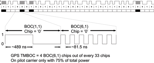
The L1C waveform originally was to have been a pure BOC(1,1) (a 1.023 MHz square wave modulated by a 1.023 MHz spreading code). Negotiations between the U.S. and the European Union (EU) at that time resulted in an agreement [6] that both GPS and Galileo would use a baseline BOC(1,1) signal. However, the EU reserved the right to further optimize their signal within certain bounds. Some of the optimization proposals were known as CBCS and CBCS. However, in further EU/US discussions it was decided that L1C and the Galileo E1 open service signal should have identically the same spectrum. This was a significant challenge because of different baseline signal structures and existing designs. The breakthrough came when Betz proposed what is called MBOC. The MBOC waveform has 10/11th of its power in BOC(1,1) and 1/11th in BOC(6,1). However, L1C and E1 OS achieve this result in very different ways. The Galileo technique is called CBOC, as described in a number of papers. [8], [9], and [10]. The GPS technique is called TMBOC and is defined by IS-GPS-800A [11] as well as by [3], [4], [5], and [8]. Whereas Galileo has a 50/50 power split between pilot and data and includes the BOC(6,1) component in each, GPS includes the BOC(6,1) waveform only in the pilot component by modulating four of every 33 spreading code chips with a 6 MHz square wave and 31 chips with a 1 MHz square wave. With 75% of the power in the pilot, the result is 3/4 x 4/33 or 1/11, as required. It is likely the BOC(6,1) signal component will be ignored by consumer grade GNSS receivers where a narrow RF bandwidth is preferred. Fortunately that is a loss of only 12% (0.56 dB) of the L1C pilot power. However, for commercial and professional grade receivers, the extra waveform transitions (wider Gabor bandwidth) can be used to improve code tracking signal-to-noise ratio, and with certain advanced techniques it should be possible to improve multipath mitigation. This final point depends on careful control or calibration of the transmitted code timing and symmetry.
Finally, Dafesh recommended that the team consider data symbol interleaving. The team accepted this suggestion, and Sklar and Wang designed the interleaver. Because of the powerful FEC, by scattering data symbols throughout sub-frames 2 and 3, it is possible to recover an entire message even if portions are blocked by, for example, walking or driving past trees or other obstructions.
All team members deserve credit for sharing, challenging, and improving concepts. Particular examples are the strong aviation navigation background provided by Hegarty and the in depth design experience for a wide range of receiver types and civilian applications provided by Keegan. In addition, Yi had the primary responsibility for documenting L1C in IS-GPS-800.
It also is important to recognize the contributions of the many professionals who responded to the worldwide survey of manufacturers, universities, and government experts. Stansell conducted each of the survey presentations, some in person and others over the Internet. One or more of the Government Chairpersons also participated, usually Hudnut or Lenahan. There were responses from organizations in 10 countries: Japan (34), the USA (26), Russia (7), the United Kingdom (5), Canada (4), Australia (1), Finland (1), Germany (1), Switzerland (1), and Taiwan (1). This is not a complete picture because a number of the responses were from individual experts while others were a consensus response from a larger group. Five signal design options were presented, and the preferred design received 62 percent of the 81 responses. As a result, the L1C signal has a 75/25 split between pilot and data power and the data rate is 50 bits per second.
L1C Signal Description
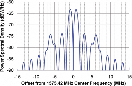
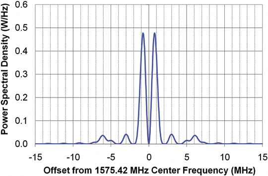
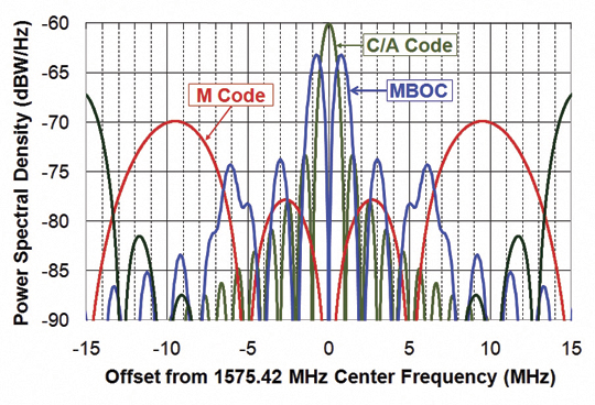
The official L1C signal description is given by IS-GPS-800; the most recent version A was released on June 8, 2010. Figures 1 and 2 show the L1C power spectral density with, respectively, a logarithmic (dBW/Hz) scale and a linear (Watts per Hz) scale. Figure 3 is the same as Figure 1 but also includes the C/A and M Code signals; it assumes both signals are transmitted with the same total power.
Figure 1.Figure 2.Figure 3.
These plots illustrate three important aspects of the L1C spectrum. First, L1C is designed to have only a small impact on reception of the legacy C/A signal. This is important for the compatibility of signals with respect to each other. A good way to evaluate the impact of one signal on another is called the Spectral Separation Coefficient (SSC), which quantifies the amount of interfering power from one signal to another, under the assumption that each signal is transmitted with the same power but with different spreading codes.
The SSC between a C/A signal and the L1C signal is –68.3 dB/Hz. The spectral separation illustrated in Figures 1, 2, and 3 assures that L1C signals will have very little impact on acquiring and tracking the legacy C/A signals. Therefore, L1C is judged to be compatible with the C/A signal.
Figure 3 also illustrates that L1C and the M Code signals have very little impact on each other. The SSC between L1C and M Code is –82.8 dB/Hz. This is important because M-Code power may be substantially higher than the civilian signals, so a larger negative SSC is important to maintaining compatibility.
The third aspect of the L1C spectrum is the additional signal power at ±6.138 MHz. This component of signal power differentiates a binary offset carrier BOC(1,1) waveform from the L1C multiplexed BOC or MBOC waveform. Exactly 1/11th of the L1C signal power is a BOC(6,1) component, whereas 9/11th of the power is a BOC(1,1) component.
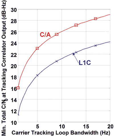
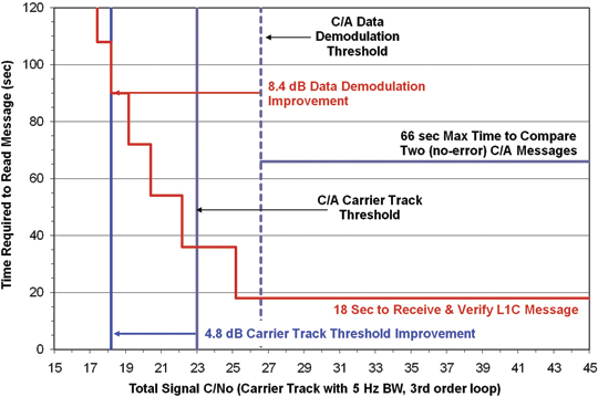
75 Percent in the Pilot Carrier. Figure 4, which shows the required post-correlator C/N0 required to phase track either the L1C or C/A signals as a function of tracking loop bandwidth, illustrates the main advantages of having 75 percent of the L1C signal power in the pilot component. The carrier-tracking threshold for equivalent signal power using a Costas loop is 6 dB worse than tracking with a phase-locked loop (PLL). A Costas loop is needed for the C/A signal because it is modulated by data, whereas a PLL can be used for the dataless L1C pilot signal. This 6 dB advantage more than compensates for having only 75 percent (-1.25 dB) of the L1C power in the pilot. The vertical displacement between the two curves illustrates the 4.75 dB L1C tracking threshold advantage.
Figure 4. Required post Correlator C/N0 versus tracking loop bandwidth.
The horizontal displacement of the curves shows another L1C advantage. For a given C/N0 threshold, the L1C loop bandwidth can be increased by a factor of three. In turn, this allows tracking with G forces 32, or nine times higher. For third-order loops capable of tracking acceleration, this allows tracking with 27 times higher jerk. Such differences are likely to be more important than tracking threshold for high-dynamic applications such as machine control.
Although Figure 4 assumes the L1C and L1 C/A signals have the same total power, the minimum received L1C signal power specified in IS-GPS-800A is –157 dBW, and the equivalent for C/A in IS-GPS-200E is –158.5 dBW. In other words, the intent is for L1C to be transmitted with 1.5 dB more power than C/A. Therefore, the figure is conservative by 1.5 dB in evaluating the L1C advantages over C/A. Thus, the actual threshold advantage is 4.75 + 1.5 = 6.25 dB.
For narrowband or other receivers not punctual correlating the BOC(6,1) signal component, the pilot carrier is 29/33 or 0.56 dB weaker, so the net advantage is 4.75 – 0.56 + 1.5 = 5.69 dB.
LDPC Block Encoding
Low-density parity check (LDPC) encoding provides three key advantages. First, to demodulate the critical part of the L1C message with a bit error rate (BER) of 10-5 requires an Eb/N0 (ratio of energy per bit to the noise power in a 1-Hz bandwidth) of 2.2 dB versus 96 dB for the C/A signal. When taking into account that only 25 percent of L1C signal power is in the data component, the required total power of the L1C signal can be 1.4 dB less than the C/A signal for an equivalent BER. As a result, this performance allows the pilot component of L1C to have 75 percent of the total L1C power.
Second, LDPC gives near-optimum performance with no intellectual property constraints. Third is the ability to block-encode Subframes 2 and 3 of the L1C message, described next.
CNAV-2 Message. Figure 5 compares the L5 and L2C CNAV message structure to the L1C CNAV-2 structure. CNAV was a major step forward compared to the original NAV message in terms of flexibility, precision, time to first fix (TTFF), and integrity. Instead of the fixed 30-second structure of the NAV message, CNAV consists of multiple six-second messages that are differentiated by a message-type number. The sequence of broadcast message types is defined by the GPS control segment, which greatly improves flexibility. The round-off error in the NAV message can affect pseudorange calculations
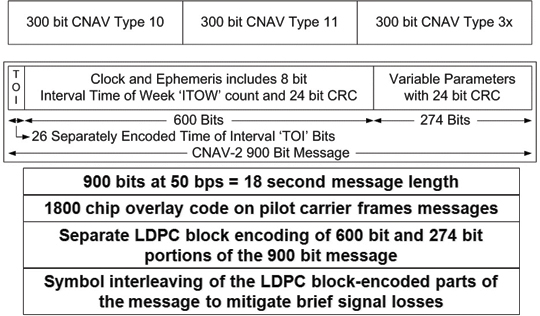
by up to 40 centimeters, whereas the equivalent CNAV error contributes about 3 centimeters. Orbit and clock precision is substantially improved. Because a minimum of three message types are needed for the necessary orbit and clock parameters, as little as 18 seconds is needed to gather the necessary information after locking to a signal. On the other hand, if four message types are being sent sequentially, and the receiver locks just after the beginning of a message, it can take 30 seconds to gather the necessary data. TTFF typically is improved. Importantly, each CNAV message includes a 24-bit cyclic redundancy check (CRC) word that makes it practically impossible to have bit errors in a message that passes the CRC check.
Figure 5. CNAV and CNAV-2 message structures.
CNAV-2 improvements to the CNAV structure all but guarantee an 18-second TTFF after signal acquisition. Message efficiency is improved by eliminating the need to identify each six-second message, to have complete time-of-week (TOW) information in each six-second message, and to have three rather than two 24-bit CRC words every 18 seconds. Even more important, GPS time is defined modulo 18 seconds upon acquisition of only one signal, and it is defined modulo two hours by decoding only one 26-bit, 0.52-second time-of-interval (TOI) word at the beginning of each message. In addition, TOI is so well encoded (52 symbols for nine data bits) that it can be demodulated in very weak signal conditions, which can be further enhanced by combining the identical TOI symbols transmitted by every satellite at the beginning of every 18-second message.
Figure 6 illustrates the ability to combine message symbols from several sequential Subframe 2 data blocks so vital clock and ephemeris data can be demodulated at the weakest signal level the receiver can track. This feature is made possible because the symbols in subframe 2 will not change for at least 15 minutes (50 repeats) and typically no more often than one to two hours (200 to 400 repeats). This provides up to 8.4 dB of message demodulation improvement. The figure also shows other L1C improvements: 4.8 dB of carrier track threshold extension, and a TTFF of 18 seconds after successfully demodulating subframe 2 from the minimum number satellites for a position fix.
Subframe 3 of the L1C message contains less time-critical information such as almanac, ionospheric correction terms, and so on. This subframe also is LDPC block-encoded so it is quite robust, although it does not offer the ability to combine symbols from sequential messages.
Figure 6. L1C and C/A performance comparison.
Pilot Overlay Code
Figure 5 shows that the pilot overlay code consists of 1,800 chips that frame the 18-second message. In comparison with the L5 20-millisecond (ms) pilot overlay code, it not only is 900 times longer but also is unique to each satellite. This improves cross-correlation performance in general and particularly when two satellites have the same pseudorange.
The long L1C overlay code can be acquired reliably after only one or two seconds of signal lock. Its length does not cause a relevant delay in TTFF, but it provides many advantages. First, synchronizing to the overlay code on one satellite defines GPS time for all satellites modulo 18 seconds (in comparison to 1 ms with the C/A code). Even with infrequent use, the receiver’s RTC, which typically is better than 5 parts per million (ppm), should have sufficient accuracy — better than ± 9 seconds — to completely resolve GPS time with one signal acquisition. In 24 hours with a clock frequency error of 5 ppm the time drift would be less than ½ second.
Even if the RTC is in error by several times 18 seconds, resolving accurate time can be done quickly by computing position fixes with multiple time hypotheses spaced 18 seconds apart. Pseudorange changes at rates up to ±1,440 kilometers per 18 seconds. Because some satellites are approaching, others are moving away, and all of them are changing range at different speeds (different Doppler frequencies), determining which position fix is correct out of several 18-second GPS time hypotheses will be straightforward since only one will be reasonable. (Care must be taken to avoid any extremely rare instances where two results may seem reasonable.)
The worst clock error with aided GPS (A-GPS) is ±2 seconds, which is adequate to completely resolve GPS time after acquiring only one L1C signal. This capability can aid acquisition of and navigation with other signals, such as C/A or signals from other GNSS providers. The 18-second overlay code will provide benefits as soon as even a few L1C signals are available.
The L1C overlay code, in conjunction with the repeating symbols of message subframe 2, also enables data demodulation to begin at any point within an 18-second message. It is not necessary to wait for the message frame to begin. The receiver can begin collecting data symbols at any time, and 18 seconds later it will have assembled all the subframe 2 clock and ephemeris information and can begin to navigate. An exception occurs when the satellite message is updated, between once every 15 minutes to once every two hours. This capability significantly improves TTFF whenever satellite messages are needed for navigation, for example, when they aren’t still valid from a previous collection or aren’t provided by an A-GPS service.
Spreading and Overlay Code Designs
The L1C MBOC waveform (time-multiplexed BOC, or TMBOC), shown in Figure 7, enabled GPS and Galileo to have open-service L1 signals with an identical spectrum, although implemented quite differently. L1C places all the BOC(6,1) chips in the pilot carrier. This is because the BOC(6,1) component is intended to improve code-tracking performance by increasing code loop signal-to-noise ratio (SNR) and by allowing advanced multipath-mitigation techniques to have the advantage of more code transitions. Because these measurements are made almost exclusively on the three times (4.8 dB) more powerful pilot signal, there is no reason to lose the code tracking benefit by having BOC(6,1) chips in the data signal component. In addition, narrowband receivers such as those predominantly used for consumer applications cannot process BOC(6,1) chips, so it would be undesirable to deny full message signal power to such receivers.
Figure 7. The GPS MBOC (TMBOC) modulation.
For receivers tracking only the BOC(1,1) component of L1C MBOC, there are on average 43.5 code transitions per 33 chips. For those tracking both components, there are on average 89.5 code transitions per 33 chips. This provides up to 3.1 dB of improvement in code loop SNR for wideband receivers code tracking with both types of chips. (The amount of improvement depends on receiver RF bandwidth.)
Classic multipath-mitigation techniques such as the double-delta don’t work well with the BOC(6,1) waveform, but recent advances promise improvement by using the extra transitions in the MBOC signal. Some developers worry that the full benefit may not be achieved unless code symmetry and time alignment of the two components is better than the signal specification permits. If the satellites cannot provide the needed signal symmetry and alignment, such problems likely can be overcome by ground calibration of these characteristics, either directly by each receiver or indirectly by an observing network.
Symbol Interleaving. Symbol interleaving means that before a message is transmitted, the satellite scatters the 10-ms message data symbols from subframes 2 and 3 throughout these subframes in
a fixed and known pattern. After a receiver has demodulated (or otherwise measured) the symbols belonging in a subframe, they are reassembled into the proper order before the LDPC block decoding is performed. In other words, the scattering done in the satellite is undone by the receiver. The objective is to provide a measure of protection against certain types of signal fading. For example, if a sequence of symbols from the satellite is lost because the receiver passes behind an object such as a tree, only half the symbols in this part of the message would be affected if the adjacent symbols in the original message are received either before or after the signal blockage. Thus, with reasonable signal levels and the benefit of powerful LDPC block encoding, the entire message could be reconstructed.
Performance Metrics and Comparison
A main objective for the L1C signal structure was to significantly improve the autonomous navigation capability for GPS users. Key weaknesses in the current C/A signal include the thresholds for bit synchronization, message synchronization, and data-bit demodulation. To achieve navigation at very low signal levels, users of the L1 C/A signal had to employ external sources for time synchronization, data acquisition, and, to extend the tracking loop threshold, external data-bit aiding to enable phase-locked tracking rather than Costas tracking of the C/A signal. The new signal structure addresses all of these shortcomings and provides a robust autonomous navigation system that requires no external aiding for most commercial applications.
Message Frame Synchronization and Time of Transmission. For autonomous navigation, frame synchronization has two important roles. The first is to set GPS time, modulo frame duration, which is required to establish the unambiguous time of transmission. Frame synchronization, or knowledge of frame start, also enables assembly of the received bits into the appropriate data words. In both L1 C/A and L5, frame synchronization is accomplished by recognizing a synch word within a data subframe, which requires accurate demodulation of data bits. For L1C, frame synchronization is inherent in the signal structure and does not require demodulation of data bits. This is very important for two reasons. The first is to establish GPS time of transmission very quickly, especially when the satellite message is not needed, for example, if it was acquired previously or obtained by other means. The second is when satellite ephemeris data is necessary, but the signals are very weak. The L1C message structure facilitates this capability.
Overlay Code on Pilot Carrier. One frame of data consists of 1,800 symbols modulated onto the data carrier which, at 100 symbols per second, is 18 seconds long. However, synchronized to this 18-second data frame is a pseudorandom code modulated on the dataless pilot carrier. This 100 chips per second overlay code is a linear-shift-register code that is truncated to be 1,800 chips long. The overlay codes were chosen to have very low minor auto-correlation and cross-correlation peaks so a very short segment of the code can be used to establish its underlying code phase.
If a 100-chip segment of the received code is correlated over a replica of the entire code, the proper correlation peak would be easily distinguished, thus establishing the GPS time epoch at the start of the code. Since this code epoch and the start of the data frame are synchronized, the start of the entire data frame is established, modulo 18 seconds. The start of the data frame by definition establishes the GPS time of transmission, also modulo 18 seconds. This is accomplished without decoding a single data bit by using the power advantage of the pilot carrier.
However, using the message to resolve the 18-second time ambiguity often is not needed. For example, the receiver’s real time clock (RTC) is likely to be accurate to within ±9 seconds. Alternately, almost any source of external aiding can provide time to within ±2 seconds. In either case, if the receiver already has a valid satellite ephemeris, navigation can begin after receiving a little over 1 second of the stronger pilot carrier signal. Ephemeris data can be available in a number of ways, including prior reception from the satellite, from a separate communications channel, or from one of several predicted ephemeris sources.
Message Frame – Data Format. A message frame consists of 1,800 symbols that comprise two distinct data types. The first data type, in subframe 1, is the Time of the Frame (TOI or Time of Interval) modulo two hours. The second data type is further separated into two blocks, subframe 2 containing data that is fixed for a period of time and subframe 3 containing data that can change from frame to frame.
Time of Interval Subframe. The TOI is a count of the number of 18-second message intervals in each 2 hour time period. Two hours is the maximum duration of any ephemeris message before being replaced by the satellite. (Fifteen minutes is the minimum.) There are 400 18-second intervals in 2 hours, so it requires 9 bits to represent the 400 intervals. These nine bits are block-encoded into 52 symbols using a BCH(51,8) code, where the 8 data bits are the least significant bits of the TOI. The most significant bit (MSB) of the TOI is then mod-2 added to the BCH codeword and also appended to the resulting codeword as its MSB, resulting in a 52-symbol codeword. This coding provides a BER of 10-5 for an Eb/N0 of –1.9 dB per coded symbol or a C/N0 of +18.2 dB-Hz at the correlator output for the data channel. Since the data channel contains only 25 percent of the total L1C power, the C/N0 of the composite signal would be +24.2 dB Hz. Symbol demodulation is performed using the pilot carrier tracked by a PLL as the phase reference. Since the pilot carrier contains 75 percent of the total power, its C/N0 would be +23 dB-Hz. With a (single-sided) loop-noise bandwidth of 10 Hz, the loop SNR for the carrier channel PLL would be +10 dB.
Note that a 10-5 BER is not required for successful demodulation of TOI. Therefore, weaker signals can be used successfully if the PLL loop bandwidth can be smaller in such weak signal conditions.
The most straightforward method to decode the TOI is brute force maximum likelihood estimation. All possible code words for the 400 possible data words can be pre-computed. Each then can be compared (correlated) with the received code word. The data word that corresponds to the code word with the highest correlation would be the result of the decoding process.
Finally, since all satellites simultaneously transmit the same TOI, the received code word from several satellites can be combined to increase the effective Eb/N0. The target BER of 10-5 thus can be achieved at an even a lower C/N0 than the single satellite value. In this case, the decoding process described above can be performed on a composite code word derived from two or more satellite signals, weighted appropriately for the signal strength from each one.
As an example, consider a receiver with access to an external source of the ephemerides. By combining the TOI code word from five satellites, the average C/N0 required per satellite would only be 17.2 dB-Hz, so time could be established to ±1 hour in slightly over 1 second.
Because of the 18-second overlay code, decoding TOI is not required for receivers with an internal clock good to ±9 seconds or with external time aiding, the worst of which today is within ±2 seconds.
Data Subframes. The remaining data bits are separated into two additional subframes. (TOI is in the first subframe.) The second subframe contains data that does not change for at least 15 minutes, and typically for an hour or two. This subframe provides the satellite ephemeris and the interval time-of-week (ITOW) count, which identifies the start time of the two-hour interval since the beginning of the GPS week, which, in turn, frames the TOI count of 18-second intervals within each two-hour frame. The third subframe contains data that normally changes from frame to frame, such as the satellite constellation almanac.
The block of data containing the satellite ephemeris (subframe-2) consists of 576 clock and ephemeris bits along with a 24-bit CRC, for a total of 600 bits. These are encoded with a rate-½ LDPC Block code into 1,200 symbols. The block of data containing variable data (subframe-3) consists of 250 data bits along with a 24-bit CRC, for a total of 274 bits. These are also encoded with a rate-½ LDPC Block code into 548 symbols. The 1,748 symbols of the two data subframes are combined and interleaved using a simple 38 x 46 row-column block interleaver. These interleaved symbols plus the 53 TOI symbols make up the entire 1,800-symbol (900-bit) message frame.
Since both the LDPC codes and the interleaver operate on independent blocks of data, the resulting symbols for subframe-2 are identical and in the same location in each message frame for between 15 minutes and two hours. Since the data decoding uses the pilot carrier as the phase reference, the subframe-2 symbols can be coherently combined over many 18-second message frames before decoding to improve BER performance.
One reasonable subframe-2 strategy would be to check the CRC after LDPC-decoding the first received message to determine if there are any remaining bit errors. If errors are detected, do the same with the second message. If errors exist in the second message, coherently combine the symbols from the two messages, properly weighted, LDPC-decode the combination, and check the resulting CRC for errors. If necessary, this process can be used on as many messages as needed to obtain a perfect result.
Framing the data messages with the pilot overlay code and the repeating characteristic of subframe 2 permits data collection over any arbitrary 18-second interval. It doesn’t matter where data collection begins. The overlay code tells the receiver which symbol is which, and the repeating subframe-2 message can be compiled from any place in the previous message to the same place in the following message. The powerful CRC assures that a good message is perfect. When the ephemeris is needed from a satellite, rather than from an alternate source, these characteristics allow TTFF to be slightly over 18 seconds, with assurance the information is correct.
Since LDPC FEC has been adopted by the current state-of-the-art wireless standards such as 802.11n and 802.16e, employing it in the latest GPS signal structure should be simple for the receiver designer. In fact, synthesizable cores are available for WiMax LDPC decoders from several sources, and LDPC decoders are as commonplace in wireless signal basebands as Viterbi decoders for the convolutional codes of L2C, L5, and SBAS have become in GPS basebands.
For subframe-2 data, the Eb/N0 required to achieve a BER of 10-5 is approximately 2.2 dB. For subframe-3 data, the Eb/N0 required for this same performance is approximately 2.7dB.
Signal Structure
The L1C signal is a composite of two signals that are phase/frequency coherent with synchronized spreading codes and symbol timing. The pilot signal has 75 percent of the total power, is a carrier-only signal, and is spread by a 10-ms long code plus an 18-second overlay code. The data signal has 25 percent of the total power, is spread by a 10-ms long code, and is data modulated with 10-ms symbols.
Spreading Codes. The spreading code for both L1C signals are 10,230 chip codes with a chip rate of 1.023 MHz, producing a 10-ms long code. This corresponds to one symbol for the data carrier and one chip of the overlay code for the pilot carrier. These codes are not linear shift register sequences like all other codes employed by GPS, but are pseudo-random sequences derived from Weil sequences of length 10223. This sequence is extended by a 7-bit sequence 0110100, which is the same for all satellites, to the required length of 10230. The location within the particular Weil sequence where the extension sequence is inserted is called the insertion index. A pair of Weil indices and a corresponding pair of insertions points then determines the pair of codes for each satellite.
Synchronization to one of these Weil-based codes can be accomplished with a standard time-domain correlator, but the number of potential hypotheses has increased by a factor of ten compared to the C/A signal. However, this is no different than time-domain correlation for an L5 code, which also are 10,230 chips long. Synchronization also can be accomplished using FFT-based frequency-domain correlation, however it does require an FFT of length 65,536 (for a standard radix-2 implementation) since the FFT must span 2 full code periods at a minimum of 2 samples per code chip (40,920).
To compare L1C frequency domain correlation with L1 C/A, a frequency search window and integration time must be hypothesized. A simple example would be a 10-ms coherent integration time and ±250 Hz frequency uncertainty. Table 3 compares the number of complex operations required for L1 C/A vs. L1C.
Table 3. Comparison of FFT-based correlation for L1C versus L1 C/A. (Click to enlarge.)
For cases where large search window uncertainties exist, and frequency domain correlation provides a computational benefit, an alternate approach to L1C synchronization would be to first obtain L1 C/A synchronization using an FFT-based search, providing frequency and 10 timing hypotheses (perhaps more with potential cross-correlations for L1 C/A). These L1C hypotheses could be tested by simple time-domain correlation that would benefit from the much better cross-correlation properties of the L1C codes.
For cases where time uncertainty is not large, a time domain search of the L1C code would be no more difficult than the equivalent for L1 C/A. For cases where the time uncertainty is small but the frequency uncertainty is large, time-domain partial-period correlations could be combined in an FFT structure that would span a large frequency uncertainty with a single time hypothesis. For example, the 10,230 chips could be separated into 62 segments, each 165 chips long. The 62 segments could then be combined using a zero filled 64-pt FFT to produce 64 full correlations spanning ±3 kHz.
MBOC Waveform. The L1C spreading code is further modulated with a code clock synchronized 1.023 MHz square wave creating the BOC(1,1) signal that forms the majority of the L1C code symbols. This produces a code that appears as a 1 MHz square wave, synchronized to the Weil-based code edge, whose polarity indicates the state of the Weil-based code chip. This BOC(1,1) sequence modulates all of the data channel chips and 29 of every 33 pilot channel chips. The other 4 out of 33 Pilot channel chips are modulated by a BOC(6,1) code symbol in which a 6 MHz square wave is used instead of the 1 MHz square wave for the BOC(1,1) chips. (Recall that ‘1’ signifies 1.023 MHz and ‘6’ signifies 6.138 MHz.) For receiver designers who choose not to punctual correlate the BOC(6,1) component of the pilot carrier, the pilot carrier power will be reduced by ~0.6 dB.
The BOC(6,1) signal component provides an opportunity for better performance of advanced multipath mitigation techniques. The presence of multipath interference not only impacts the code-tracking process of a GPS receiver but also distorts the waveform seen by the phase-tracking process of the receiver. The distortion of the phase of the received signal is most problematic when the reflector creating the multipath signal is very close to the receiving antenna, because the path length of such a multipath signal changes very slowly. Since the path length changes very slowly, it appears as an almost constant bias error in the phase measurements. The only way to observe this distortion, and hence measure its impact on the phase measurements, is to observe the phase of the carrier very close to the code transitions. The estimate of this distortion obviously is better the more frequently it can be observed. This is particularly important because the distortion is not constant but slowly changes. The MBOC signal combination provides
just over twice the number of transitions at which to observe the phase distortion than the BOC(1,1) signal alone, which is important for higher fidelity measurements during short intervals when the slowly changing distortion is highly correlated .
L1C Status
Companies already are designing L1C into their new chipsets, even though the first satellite to carry the signal is not expected before 2014. When will L1C be available from enough satellites to be meaningful? Figure 8 is a guesstimate of how modernized GPS signals will become available over the next decade. The projections assume either two or three successful satellite launches per year, and many observers think two per year may be realistic. Because GPS only launches on need to sustain the constellation, the actual launch rate depends on the lifetime of the satellites now in orbit. The first launch of a GPS III may be delayed until all IIF satellites have been launched, or the first GPS III, if available, may be launched before the last IIF to test the new design in space as soon as possible.
Some L1C signal and message characteristics will significantly benefit users of C/A and other GNSS signals by, for example, quickly resolving time for all GNSS signals. Therefore, L1C will provide meaningful benefit as soon as even one signal can be tracked from any location on earth. That might be possible with as few as six GPS III satellites in orbit, depending on where in the constellation they are deployed.
Figure 8. Guesstimate of modernized GPS signal availability.
Tom Stansell heads Stansell Consulting, after eight years with the Johns Hopkins Applied Physics Laboratory, 25 years with Magnavox (staff VP), and five years with Leica Geosystems (VP), pioneering Transit and GPS navigation and survey products. He led technical development of the GPS L2C signal and coordinated the GPS L1C project (2004–2006). He is a member of the Editorial Advisory Board of GPS World.
Ken Hudnut applies new technologies such as GPS to earthquake research as a geophysicist for the U. S. Geological Survey in Pasadena, California. He served as project manager for the GPS L1C signal design project from 2003. He received his Ph.D. from Columbia University.
Rich Keegan has 36 years of experience in radio navigation including Transit, Timation, Omega, Loran C, as well as GPS for the past 28 years. He has been the principal of a consultancy in digital communications and navigation since 2000. He was a member of the L2C and L1C modernization committees.
The Galileo Test and Development Environment (GATE) in Berchtesgaden, Germany, officially opened on February 4. The system operator, IFEN GmbH of Poing, Germany, jointly with the German Federal Minister of Transport, Building and Urban Development, announced the opening for use by commercial and organizational entities seeking to test equipment with the coming Galileo signals. GATE was developed on behalf of the German Aerospace Center (DLR) with funding by the German Federal Ministry of Economics and Technology.
The test area extends across a valley of approximately 65 square kilometers, south-east of Munich, where antennae atop surrounding peaks broadcast the various Galileo signals. Technical details and specifications of the test environment are at www.gate-testbed.com.
GATE has completed its signal upgrade phase according to the latest version of the European Space Agency’s Galileo Signal-In-Space (SIS) Interface Control Document (ICD) and the European GNSS Agency’s Public Galileo Open Service (OS) ICD. The GATE infrastructure is capable of transmitting the Galileo OS, the Galileo Safety-of-Life (SoL) Service (functional), the Galileo Commercial Service (CS), and a Galileo Public Regulated Service (PRS) dummy signal.
The GATE system upgrade has been further extended to also support user integrity testing. GATE can simulating simple alarm-triggering events on the system/satellite level, supporting GPS and GATE/Galileo dual-constellation receiver-autonomous integrity monitoring (RAIM), individual user integrity test scenarios, and tests of receivers with different RAIM functionalities.
The next step will be certification of the GATE test infrastructure as an officially accredited open-air test infrastructure to perform the necessary tests needed for the process to certify Galileo SoL equipment.
Günter Heinrichs, head of customer applications and business development for IfEN GmbH, described the goals and capabilities of GATE in a 2007 GPS World article. He gave an update on developments in a 2009 video interview. A recent simulation of emergency response scenarios using the Galileo signal is described at Galileo to the Rescue.
By Cillian O’Driscoll, Gérard Lachapelle, and Mohamed Tamazin, University of Calgary
The impact of adding GLONASS to HS-GPS is assessed using a software receiver operating in an actual urban canyon environment. Results are compared with standard and high sensitivity GNSS receivers and show a significant improvement in the availability of position solutions when GLONASS is added. An assisted high sensitivity receiver architecture is introduced which enables high fidelity signal measurements even in degraded environments.
High-sensitivity (HS) GNSS receivers have flourished in the last decade. A variety of advances in signal-processing techniques and technologies have led to a thousandfold decrease in the minimum useable signal power, permitting use of GNSS, in particular GPS, in many environments where it was previously impossible.
Despite these recent advances, the issue of availability remains: in many scenarios there are simply too few satellites in view with detectable signals and a good geometry to compute a position solution. Of course, one way to improve this situation is to increase the number of satellites in view. GLONASS has been undergoing an accelerated revitalization program of late, such that there are currently more than 20 active GLONASS satellites on orbit. The combined use of GPS and GLONASS in a high-sensitivity receiver is a logical one, providing a near two-thirds increase in the number of satellites available for use.
The urban canyon environment is one in which the issue of signal availability is particularly important. The presence of large buildings leads to frequent shadowing of signals, which can only be overcome by increasing the number of satellites in the sky. Even if sufficient satellites are visible, the geometric dilution of precision can often be large, leading to large errors in position.
This work focuses on the advantages of using a combined GPS/GLONASS receiver in comparison to a GPS-only receiver in urban canyons. The target application is location-based services, so only single frequency (L1) operation is considered. We collected and assessed vehicular kinematic data in a typical North American urban canyon, using a commercially available high-sensitivity GPS-only receiver, a commercial survey-grade GPS/GLONASS receiver, and a state-of-the-art software receiver capable of processing both GPS and GLONASS in standard or high-sensitivity modes.
Processing Strategies
The standard (scalar-tracking) GNSS receiver architecture is shown in Figure 1. In the context of this article, the key characteristic of a standard receiver is that the signals from the different satellites are each tracked in parallel and independent tracking channels, and usually only three correlators are used. The information from the channels is only combined in the navigation filter to estimate position, velocity, and time. In this way, there is no sharing of information between channels in order to attempt to improve tracking performance.
Figure 1. Standard receiver architecture (courtesy Petovello et al).
Within each channel, the down-converted and filtered samples from the front end (not shown in Figure 1) are then passed to a signal-processing function where Doppler-removal (baseband mixing) and correlation (de-spreading) is performed. The correlator outputs are then passed to an error-determination function consisting of discriminators (typically one for code, frequency, and phase) and loop filters. The loop filters aim to remove noise from the discriminator outputs without affecting the desired signal. Finally, the local signal generators — whose output is used during Doppler removal and correlation — are updated using the loop-filter output.
Assisted HS GNSS Receiver. The assisted HS GNSS receiver architecture used in this work is shown in Figure 2. Notable differences to the standard receiver architecture are highlighted in red.
Assistance information is provided in the form of broadcast ephemerides, raw data bits, and a nominal trajectory (position and velocity) that would normally be generated by the receiver. At each measurement epoch, the receiver uses the nominal position and velocity in conjunction with the ephemerides to compute the nominal pseudorange and pseudorange rate for each satellite in view. These parameters are passed to the signal-processing channels. Each channel evaluates a grid of correlators around the nominal pseudorange (code) and pseudorange rate (Doppler) values. The data bits are wiped off using the assistance information to permit long coherent integration times. For each signal tracked, the correlator grid is used to estimate code and Doppler offsets relative to the nominal values. These estimates are then used to generate accurate pseudorange and Doppler estimates.
The number of correlators used and the spacing of these correlators in the code and frequency domains are completely configurable. A sample correlation grid computed during live data processing is illustrated in Figure 3. Measurements are generated by choosing the three correlators nearest the peak in the search space and using a quadratic fit to determine a better estimate of the peak location. In this work, a total of 55 correlators per channel were used.
Figure 3. Sample grid of correlator points computed for GPS PRN 04.
The assisted HS receiver is initialized in static mode in an open-sky setting during which reliable clock bias and drift estimates are derived. A high-quality oven-controlled crystal oscillator was used during this initial test to ensure that the clock drift did not change significantly over the period of the test (approximately 20 minutes). The clock bias during the test is updated using the clock drift estimate.
Note that this architecture is a generalization of the vector-based architecture, where the navigation solution used to aid the signal processing can be provided by an external reference.
Navigation Solution Processing. All navigation solution results presented here are obtained in single-point mode using an epoch-by-epoch least-squares solution with the PLAN Group C3NavG2 software, which uses both code and Doppler measurements. This processing strategy enables a fair comparison amongst the different signal processing strategies, as the smoothing effect of specific navigation filters is eliminated by this approach. More realistic accuracy estimates of the measured pseudoranges can be obtained. It is understood that in an operational environment, a well-tuned filter will obtain significantly better navigation performance than the epoch-by-epoch solutions presented here.
The measurements are weighted using a standard-elevation-dependent scheme. Thus there is no attempt to tune the weighting scheme for each receiver.
Data Collection
To test the relative performance of the various processing strategies, we conducted a test in downtown Calgary. Data was collected using a commercial HS GPS receiver, a commercial survey grade GPS/GLONASS receiver, and an RF downconverter and digitizer. The digitized data was post-processed in two modes (standard and assisted HS GNSS) using the PLAN group software receiver GSNRx.
Raw measurements were logged from each of the commercial receivers at a 1-second interval. The parameters used in GSNRx are given in Table 1.
The trajectory followed is shown in Figure 4. The majority of the route was travelled in an East-West direction, with significant signal masking to the North and South. The Opening Photo shows an aerial view of downtown Calgary where the test took place. Masking angles exceeded 75 degrees along the vehicle trajectory.
Figure 4. Test Trajectory where the route is approximately 4 km with a 10 minute travel time.
A sky plot of the satellites visible above a 5-degree elevation mask at the test location is shown in Figure 5. A total of 11 GPS and seven GLONASS satellites were present.
Figure 5. Skyplot of GPS and GLONASS satellites over Calgary at the start of the test.
A static period of approximately three minutes duration was used to initialize the assisted HS GNSS processing. During this period, the vehicle had a largely clear view of the sky. Nevertheless, three satellites were blocked from view during this period, namely GPS SVs 13 and 3, and GLONASS SV 22. As a result, these SVs were not available for processing in the assisted HS GNSS mode. The two commercial receivers were already up and running prior to the initialization period and so were able to process these three low-elevation satellites when they came into view during the test. See PHOTO on next page for a typical scene during the downtown test.
Analysis
To study the impact of adding GLONASS, the analysis focuses on solution availability, the number of satellites used in each solution, the DOP associated with each solution, and the statistics of the least-squares solution residuals. In the absence of a reference solution, the statistics of the residuals nevertheless give a reasonable indication of the quality of the measurements used, provided sufficient measurements are available to ensure redundancy in the solution. Nevertheless, some pseudorange errors will be absorbed by the navigation solution, hence the statistics of the residuals can be viewed as only a good estimate of the quality of the measurements themselves.
Solution Availability. As previously discussed, the navigation processing strategy adopted is the same for all receivers used in the test. A single-point epoch-by-epoch least-squares solution is computed at a 1 Hz rate. If there are insufficient satellites in view at a given epoch, or the solution fails to converge in 10 iterations, no solution is computed. In this section, the analysis focuses on the percentage of epochs during the downtown portion of the test for which a solution was computed.
Figure 6 shows the percentage of solutions computed for each receiver processing strategy as a function of HDOP and VDOP thresholds, respectively. Thus, for example, the assisted HS GPS-GLONASS processing strategy yielded navigation solutions with a HDOP less than 6 between 80 percent and 85 percent of the time. For larger DOP thresholds, it is clear that there is little difference between GPS-only processing and GPS+GLONASS processing. The biggest differences are caused by the processing strategies employed. The advantages of HS processing are clear, at least in terms of solution availability. For this test and the particular geometry of the satellites in view during the test, GPS+GLONASS processing does yield a noticeable improvement in the VDOP, particularly at lower thresholds.
Figure 6A. Percentage solution availability versus HDOP threshold.Figure 6B. Percentage solution availability versus VDOP threshold.
Note that the standalone HS GPS receiver exhibits greater solution availability than the assisted software HS GPS-GLONASS receiver at higher DOP thresholds. This is most likely due to the low-elevation satellites that were excluded from the assisted HS processing due to their being masked during the initialization period as discussed earlier. Overall, however, there is little difference between GPS-only processing and GPS-GLONASS processing in terms of solution availability. This fact, of course, does not yield any information on the quality of the solutions obtained, which is discussed later.
To gain further insight into the impact of GLONASS, Figure 7 shows the percentage of solutions computed that exhibit redundancy. Thus, of all solutions computed during the downtown portion of the test, Figure 7 illustrates the percentage of those solutions that have redundant measurements. For GPS-only processing, this implies that five or more measurements were used in computing the position, while for GPS-GLONASS processing a minimum of six measurements were required. In this case, the advantage of using GLONASS becomes more apparent. For all processing strategies the addition of GLONASS yields an increase of 5 to 10 percent in the number of solutions with redundancy. Although not studied herein, this would have a positive impact on fault detection.
Residuals Analysis
To investigate the quality of the measurements generated by each processing strategy, the residuals from the least-squares solutions are studied. Only those epochs for which redundant solutions are computed are considered here, since non-redundant solutions lead to residuals with values of zero. As discussed above, the analysis of these residuals gives an estimate of the quality of the measurements generated.
Figure 8 shows the histograms of the residuals from all GPS-GLONASS processing strategies. Once again, it is important to emphasize that only residuals from solutions with redundancy are considered. In addition, the results presented are limited to those epochs during which the vehicle was in the downtown portion of the test. For the purposes of this presentation an upper GDOP threshold of 10 was set.
It is interesting to note that in all cases (assisted HS, standard wide correlator, and commercial survey-grade processing), the relative RMS values of the GPS and GLONASS residuals are about the same. These results indicate that, irrespective of the signal-processing strategy employed, the GLONASS measurements are of a similar quality to the GPS measurements. The number of residuals available is however different between the standard and HS solutions, as the latter produce more measurements and more redundant solutions, hence more residuals. The processing strategy obviously had a significant impact on the availability of redundant solutions as discussed in the previous section.
Figure 8A. GPS-GLONASS range residuals comparison: assisted HS-GPS-GLONASS. RMS values and the percentage of solutions used in the histogram are also shown.Figure 8B. GPS-GLONASS range residuals comparison: standard wide correlator. RMS values and the percentage of solutions used in the histogram are also shown.Figure 8C. GPS-GLONASS range residuals comparison: survey-grade receiver. RMS values and the percentage of solutions used in the histogram are also shown.
Figure 9 shows the histograms of the range residuals from GPS-only processing. In this case, the navigation solution is a GPS-only navigation solution, though in the case of the assisted HS receiver the measurements used are identical to those used in Figure 8.
Clearly the assisted HS receiver has a greater availability of redundant solutions compared to the standalone receiver, which is to be expected. Also, the assisted HS GPS receiver residuals have a slighter lower RMS than when a GPS-GLONASS implementation was considered, indicating that the navigation solution absorbs more of the measurement errors in this case.
Figure 9A. GPS range residuals comparison, assisted HS GPS.Figure 9B. GPS range residuals comparison, commercial standalone HS GPS.
Position Domain Results
The final stage of the analysis is a comparison of the trajectories computed using each of the receiver types. While no truth solution was available for this test, a highly filtered navigation solution from the high-sensitivity commercial receiver was used as a nominal reference. This trajectory is shown in black in the following figures.
Figure 10 shows the trajectories obtained using standard wide-correlator processing. The position solutions are quite accurate, but the availability is low, namely of the order of 30 percent as shown above. The addition of GLONASS does improve the availability in this case. The accuracy is not significantly improved. In fact it appears that the addition of GLONASS occasionally leads to biases in the navigation solutions, likely solutions with high DOP values.
Figure 10. Trajectory obtained with standard wide correlator processing.
Figure 11 shows the trajectories computed using the commercial receivers. The survey-grade receiver yields less noisy positions, though the addition of GLONASS does lead to some significant outliers. The position availability is lower as discussed earlier. Similar to the standard wide-correlator processing case, the addition of GLONASS again appears to introduce an error in the solution during some epochs (for example, at a northing of about 500 meters between 100 and 500 meters easting).
Figure 11. Trajectories obtained from the commercial receivers.
Finally, Figure 12 shows the trajectories obtained from the assisted HS receiver. In this case, the position solutions are significantly less noisy than in previous cases, in addition to being more available. The quality of the GPS-only and GPS+GLONASS results is broadly similar, with perhaps more outliers in the GPS-GLONASS case, due to the reason mentioned earlier.
Figure 12. Trajectories obtained using assisted HS GPS-GLONASS processing.
In summary, it would appear that the greatest benefit of GLONASS in this test was in the provision of greater redundancy in the navigation solution, in addition to potential better reliability, although the latter remains to be confirmed. With GLONASS approaching full operational capability, it is to be expected that the increased GLONASS constellation will lead to further improvements in terms of availability, DOP, and reliability.
Coherent Integration Time
From the preceding analysis it is clear that the assisted HS GNSS processing strategy yielded the best performance. To evaluate the impact of the coherent integration time on performance, the data was re-processed with a coherent integration time of 300 milliseconds (ms), instead of the 100 ms used for the data presented so far. The resulting trajectories are shown in Figure 13.
It is interesting to note that increasing the receiver sensitivity in this way does not yield better navigation performance. In fact, in the urban canyon environment, the major issue is not the signal attenuation (which can be overcome by increased coherent integration) but rather the multipath effect. By increasing the coherent integration time to 300 ms, the receiver becomes more sensitive to dynamics, resulting in poorer navigation performance.
Figure 13. Trajectories obtained using assisted HS GPS-GLONASS processing (300 ms integration time).
Discussion
High-sensitivity processing in urban canyon environments is a very effective means of improving navigation performance. Given the discussion above, however, it is clear that the performance is not limited by the strength of the received signal, but rather by the effect of multipath and satellite geometry.
The advantage of high-sensitivity processing in this case is two-fold. The first advantage over standard tracking techniques is the open-loop nature of HS processing. The time-varying nature of the multipath channel causes significant variation in signal level. This variation can cause traditional tracking loops to lose lock. In fact, the poor performance of the standard wide-correlator strategy in the above analysis can be explained by the fact that the receiver was unable to maintain lock on the satellites in view. Hence no measurements were generated, and no solutions computed. The survey-grade receiver used has advanced multipath mitigation technology, which helped to avoid loss of lock, but may have been tracking non-line-of-sight signals during portion of the down-town test, leading to errors in the navigation solution.
The second advantage of HS processing is related to the coherent integration time and the vehicle dynamics. As the receiver antenna moves through the multipath environment, a different Doppler shift is observed on signals coming from different directions. Thus the line-of-sight and multipath components become separated in frequency. A longer coherent integration time increases the frequency resolution of the correlator output (due to the familiar sinc shape). Thus if the line-of-sight is present, and the coherent integration time is long relative to the inverse of the Doppler difference between the line-of-sight and reflected signals, individual peaks become visible in the grid of correlators. This effect can significantly reduce the impact of multipath on the measurements. Figure 14 gives an example of this.
Figure 14. Sample correlation function showing two peaks.
Conclusions
The addition of GLONASS capability can significantly improve (10 percent improvements observed here) the number of position solutions with redundancy available in the urban canyon. With increasing GLONASS satellite availability, the benefits of using GLONASS will even be greater. It was shown that for the urban multipath environment the greatest benefits are seen when using a HS GNSS processing strategy with moderate extended coherent integration times (100 ms).
Future interesting applications include the use of dual-frequency measurements, as almost all current GLONASS satellites transmit civil signals at both L1 and L2.
Acknowledgments
The authors would like to kindly acknowledge and thank Defence Research and Development Canada (DRDC) for partly funding this work.
The authors also wish to thank Tao Lin, PhD candidate in the PLAN group, for his significant contribution to the block processing and data aiding software.
Manufacturers
The tests used a National Instruments PXI-5661 RF downconverter and digitizer, the PLAN GSNRx as standard wide-correlator receiver, the u-blox Antaris 4 (standalone HS-GPS), NovAtel OEMV-3 (survey-grade GPS/GLONASS), and the PLAN group software receiver GSNRx, as the assisted HS GPS/GLONASS.
Cillian O’Driscoll received his Ph.D. in 2007 from the Department of Electrical and Electronic Engineering, University College Cork, and is currently a post-doctoral fellow in the PLAN Group of the University of Calgary.
Gérard Lachapelle is a professor of geomatics engineering at the University of Calgary where he holds a Canada Research Chair in wireless location and heads the Position, Location and Navigation (PLAN) Group.
Mohamed Tamazin is a M.Sc. candidate in the the PLAN at the University of Calgary. He holds a M.Sc. in electrical communications from the Arab Academy for Science and Technology, Alexandria, Egypt.
By John Nielsen, Ali Broumandan, and Gérard Lachapelle
Ubiquitous adoption of and reliance upon GPS makes national and commercial infrastructures increasingly vulnerable to attack by criminals, terrorists, or hackers. Some GNSS signals such as GPS P(Y) and M-code, GLONASS P-code, and Galileo’s Public Regulated Service have been encrypted to deny unauthorized access; however, the security threat of corruption of civilian GNSS signals increases constantly and remains an unsolved problem. We present here an efficient approach for the detection and mitigation of spoofed GNSS signals, as a proposed countermeasure to add to the existing system.
Current methods to protect GPS civilian receivers from spoofing signals are based on the cross-check with available internal/external information such as predictable characteristics of the navigation data bits or correlation with ancillary inertial-based sensors; alternately, a joint process of signals received at two separate locations based on processing the P(Y)-code.
The authentic GNSS signal sourced from a satellite space vehicle (SV) is very weak at the receiver’s location and is therefore vulnerable to hostile jamming based on narrowband noise radiation at a modest power level. As the GNSS frequency band is known to the jammer, the effectiveness of the latter is easily optimized by confining radiation to within the GNSS signal band. The jammed GNSS receiver is denied position or time estimates which can be critical to the mission. While noise jamming of the GNSS receiver is a threat, the user is easily aware of its existence and characteristics. The worst case is that GNSS-based navigation is denied.
A more significant jamming threat currently emerging is that of the spoofing jammer where bogus signals are transmitted from the jammer that emulate authentic GNSS signals. This is done with multiple SV signals in a coordinated fashion to synthesize a plausible navigation solution to the GNSS receiver. There are several means of detecting such spoofing jammers, such as amplitude discrimination, time-of-arrival discrimination, consistency of navigation inertial measurement unit (IMU) cross-check, polarization discrimination, angle-of-arrival (AOA) discrimination, and cryptographic authentication.
Among these authentication approaches, the AOA discriminator and spatial processing have been addressed and utilized widely to recognize and mitigate hostile attacks. We focus here on the antenna-array processing problem in the context of spoofing detection, with considerations to the pros and cons of the AOA discriminator for handheld GNSS receivers.
An exploitable weakness of the spoofing jammer is that for practical deployment reasons, the spoofing signals generally come from a common transmitter source. Hence, a single jamming antenna sources the spoofing signals simultaneously. This results in a means of possible discrimination between the real and bogus GNSS signals, as the authentic GNSS signals will emanate from known bearings distributed across the hemisphere.
Furthermore, the bearing of the jammer as seen from the GNSS receiver will be different than the bearing to any of the tracked GNSS satellites or space vehicles (SV). This immediately sets up some opportunities for the receiver to reject the spoofing jamming signals. Processing can be built into the receiver that estimates the bearing of each SV signal. Note that the relative bearings of the GNSS signals are sufficient in this case, as the bogus signals will all have a common bearing while the authentic GNSS signals will always be at different bearings.
If the receiver comprises multiple antennas that have an unobstructed line of sight (LOS) to the SVs, then there are possibilities of spoofing detection based on the common bearing of the received GNSS signals and eliminating all the jammer signals simultaneously by appropriate combining of the receiver antennas to form a pattern null coincident with the jammer bearing.
Unfortunately, the AOA discrimination will not be an option if the jammer signal or authentic signals are subjected to spatial multipath fading. In this case, the jammer and individual SV signals will come in from several random bearings simultaneously. Furthermore, if the GNSS receiver is constrained by the form factor of a small handset device, an antenna array will not be an option. As the carrier wavelength of GNSS signals is on the order of 20 to 25 centimeters, at most two antennas can be considered for the handset receiver, which can be viewed as an interferometer with some ability of relative signal-bearing estimation as well as nulling at specific bearings.
However, such an antenna pair is not well represented by independent isotropic field sampling nodes, but will be significantly coupled and strongly influenced by the arbitrary orientation that the user imposes. Hence, the handset antenna is poorly suited for discrimination of the spoofing signal based on bearing. Furthermore, handheld receivers are typically used in areas of multipath or foliage attenuation, and therefore the SV signal bearing is random with significant variations.
As we discuss here, effective spoofing detection is still possible for a single antenna GNSS receiver based on the differing spatial correlation of the spoofing and authentic signals in the proximity of the receiver antenna. The basic assumption is that the antenna will be spatially moved while collecting GNSS signal snapshots. Hence, the moving antenna generates a signal snapshot output similar to that of a synthetic array (SA), which, under some additional constraints, can provide an effective means of detecting the source of the GNSS signals from a spoofing jammer or from an authentic set of SVs.
We assume here an arbitrary antenna trajectory with the spoofing and authentic signals subjected to random spatial multipath fading. The processing will be based on exploiting the difference in the spatial correlation of the spoofing and the authentic signals.
Spoofing Detection Principle
Consider a GNSS handset receiver (Figure 1) consisting of a single antenna that is spatially translated in time along an arbitrary trajectory as the signal is processed by the GNSS receiver. There are L authentic GNSS SV signals visible to the receiver, along with a jammer source that transmits spoofing replicas of the same Lauthentic signals.
FIGURE 1. GNSS receiver with a single antenna and 2L parallel despreading channels simultaneously providing channel gain estimates of L authentic and L spoofing signals as the antenna is moved along an arbitrary spatial trajectory.
It is assumed that the number of spoofed signals range from 1 to L, which are coordinated such that they correspond to a realistic navigation solution at the output of the receiver processing. The code delay and Doppler associated with the spoofing signals will typically be different than those of the authentic signal. The basic technique of coordinated spoofing jamming is to present the receiver with a set of L signals that appear to be sufficiently authentic such that the spoofing and authentic signal sets are indistinguishable. Then the spoofing signals separate slowly in terms of code delay and Doppler such that the navigation solution corresponding to the L spoofing signals will pull away from the authentic navigation solution.
The focus herein is on methods where the authenticity of the L tracked GNSS signals can be tested directly by the standalone receiver and then selected for the navigation processing. This is in contrast with other methods where the received signals are transmitted back to a communication command center for verification of authenticity. The consideration here is on the binary detection problem of assessing if each of the 2L potential signals is authenti
c or generated by a spoofing source. This decision is based on observations of the potential 2L GNSS signals as the antenna is spatially moved through the trajectory.
The complex baseband signal at the output of the antenna, denoted by r(t), can be expressed as
where i is the GNSS signal index, the superscripts A and J indicate authentic and jamming signals respectively, p(t) shows the physical position vector of the moving antenna phase center relative to a stationary spatial coordinate system, ΛAi(p(t),t) and ΛJi(p(t),t) give the channel gain for the authentic and the spoofing signals of the ith SV at time t and position p, ci(t) is the PN coding modulation of ith GNSS signal, πAi and πJi are the code delay of ith PN sequence corresponding to the authentic and the spoofing sources respectively, fDiA and fDiJ are the Doppler frequency of the ith authentic and the spoofing signals and w(t) represents the complex baseband of additive noise of receiver antenna. For convenience, it is assumed that the signal index iε[1, 2,…,L] is the same for the spoofing and authentic GNSS signals. The spoofer being aware of which signals are potentially visible to the receiver will transmit up to L different spoofing signals out of this set.
Another simplification that is implied by Equation 1 is that the message coding has been ignored, which is justifiable as the GNSS signals are being tracked such that the message symbol modulation can be assumed to be removable by the receiver by some ancillary process that is not of interest in the present context. The objective of the receiver despreading operation is to isolate the channel gains ΛA(p(t),t) ΛJ(p(t),t), which are raw observables used in the subsequent detection algorithm.
It is assumed that the GNSS receiver is in a signal tracking state. Hence, it is assumed that the data coding, code phase of the spreading signal and Doppler are known inputs in the despreading operation. The two outcomes of the ith despreading channel for authentic and jamming signals are denoted as riA(t) and rkJ(t) respectively, as shown in Figure 1. This notation is used for convenience and not to imply that the receiver has knowledge of which of the pair of GNSS signals corresponds to the authentic or spoofer cases. The receiver processing will test each signal for authenticity to select the set of L signals that are passed to the navigation estimator.
The despread signals riA(t) and rkJ(t) are collected over a snapshot interval of tε[0,T]. As the notation is simplified if discrete samples are considered, this interval is divided into M subintervals each of duration ΔT such that the mth subinterval extends over the interval of [(m−1)ΔT,mΔT]for mε[1,,2,…,M]. The collection of signal over the first and mth subintervals is illustrated in Figure 2. ΔT is considered to be sufficiently small such that ΛAi(p(t),t) or ΛJk(p(t),t) is approximately constant over this interval leading a set of M discrete samples for each despreading output. From this the vectors form of channel gain sample and outputs of despreaders can be defined by
where ΛAi(p(mΔT),mΔT) and ΛJi(p(mΔT),mΔT) are the mth time sample of the ith despreader channel for the authentic and jamming GNSS signals.
Figure 2. Spatial sampling of the antenna trajectory into M subinterval segments.
Pairwise Correlation
The central tenet of the spoofing detection is that the array gain vector denoted here as the array manifold vector for the jammer signals ΛJ will be the same for all of the L spoofing signals while the array manifold vector for the authentic signals ΛA will be different for each of the L authentic signals. If the random antenna trajectory is of sufficient length, then the authentic signal array manifold vectors will be uncorrelated. On the other hand, as the jammer signals emerge from the same source they will all have the same array manifold vector regardless of the random antenna trajectory and also regardless of the spatial fading condition. This would indicate that a method of detecting that a spoofer is present to form the Mx2L matrix of all of the despreader output vectors denoted as r and given as
where it is assumed that M≥2L.
Basically what can be assumed is that, if there is a spoofer from a common source that transmits more than one GNSS signal simultaneously, there will be some residual spatial correlation of the observables of ΛJi with other despreader outputs of the receiver. Therefore, if operations of pairwise correlations of all of the 2L despreader outputs result in high correlation, there is a likelihood of the existence of spoofing signals. These pairwise correlations can also be used to distinguish spoofing from authentic signals. Note that even during the time when the spoofing and authentic signals have the same Doppler and code offset, the superposition manifold vector of ΛAi and ΛJi will be correlated with other spoofing manifold vectors. The pairwise correlation of the various spoofing signals can be quantified based on the standard numerical estimate of the correlation coefficient given as
where ri is the ith column vector of r defined in Equation 3, and the superscript H denotes the complex conjugate operator.
Toward Spoofing Detection
Figure 3 shows the spoofing attack detection and mitigation methodology:
The receiver starts with the acquisition process of a given GNSS code. If, for each PN sequence, there is more than one strong peak above the acquisition threshold, the system goes to an alert state and declares a potential spoofing attack. Then the receiver starts parallel tracking on each individual signal.
The outputs of the tracking pass to the discriminator to measure the correlation coefficient ρ among different PN sequences. As shown in Figure 3, if ρ is greater than a predefined threshold ϒ, the receiver goes to defensive mode. As the spoofer attempts to pull the tracking point off the authentic signals, the spoofer and authentic signals for a period of time will have approximately the same code offset and Doppler frequency. Hence, it may not be possib
le to detect more than one peak in the acquisition mode. However, after a while the spoofer tries to pull tracking mode off.
The outputs of the parallel tracking can be divided into two groups: the J group is the data set that is highly correlated, and the A group is the set that is uncorrelated. It is necessary that the receiver antenna trajectory be of sufficient length (a few tens of the carrier wavelengths) such that M is moderately large to provide a reasonable estimate of the pairwise correlation.
The A group will be constrained in size based on the number of observable satellites. Usually this is known, and L can be set. The receiver has control over this by setting the bank of despreaders. If an SV signal is known to be unobtainable due to its position in the sky, it is eliminated by the receiver. Hence the A group can be assumed to be constrained in size to L. There is the possibility that a spoofer will generate a signal that is clear, while the SV signal is obscured by shadowing obstacles. Hence a spoofing signal can inadvertently be placed in the A group. However, as this signal will be correlated with other signals in the J group, it can be transferred from the A to the J group.
When the spoofing navigation solution pulls sufficiently away from the authentic solution, then the navigation solution can create two solutions, one corresponding to the authentic signals and the other corresponding to the spoofing signals. At this stage, the despreading code delay and Doppler will change such that the authentic and spoofing signals (corresponding to the same GNSS signal) will appear to be orthogonal to each other.
Proper placement of the members in the J and A groups can be reassessed as the set of members in the A group should provide the minimum navigation solution variance. Hence, in general there will be a spoofing and authentic signal that corresponds to the GNSS signal of index i. If the spoofing signal in group J appears to have marginal correlation with its peer in group A and, when interchanged with its corresponding signal in group A, the latter generates a lower solution variance, then the exchange is confirmed.
Figure 3. Spoofing detection and mitigation methodology.
Experimental Measurements
We used two data collection scenarios in experiments of spoofing detection, based on utilizing a single antenna that is spatially translated, to demonstrate the practicality of spoofing-signal detection based on spatial signal correlation discrimination. In the first scenario, the spoofing measurements were conducted inside a modern three-story commercial building. The spoofing signals were generated by a hardware simulator (HWS) and radiated for a few minutes indoors, using a directional antenna pointing downward to affect only a small area of the building. The intention was to generate NLOS propagation conditions with significant multipath.
The second data collection scenario was based on measuring authentic GPS L1 C/A signals under open-sky conditions, in which case the authentic GPS signals are temporally highly correlated. At the particular instance of the spoofing and the authentic GPS signal measurement scenarios, the SVs were distributed as shown in Figure 4. The GPS receiver in both scenarios consisted of an active patch right-hand circular polarized (RHCP) antenna and a down-conversion channelizer receiver that sampled the raw complex baseband signal. The total data record was subsequently processed and consisted in acquiring the correlation peaks based on 20-millisecond coherent integration of the spoofing signals and in extracting the channel gains L as a function of time.
Figure 4. Skyplots of available satellites: a) spoofing signals from Spirent generator, b) authentic signals from rooftop antenna.
Figure 5 shows a plot of the samples of the magnitude of despreader outputs for the various SV signals generated by the spoofing jammer and authentic signals. The signal magnitudes in the spoofing case are obviously highly correlated as expected, since the jammer signals are all emanating from a common antenna. Also, the SNRs are moderately high such that the decorrelation due to the channel noise is not significant.
The pairwise correlation coefficient using Equation 4 are calculated for the measurement results represented in Figure 5 and tabulated in Table 1 and Table 2 for the spoofing and the authentic cases respectively. As evident, and expected, the correlations for the spoofing case are all very high. This is anticipated, as the spoofing signals all occupy the same frequency band with exception of small incidental shifts due to SV Doppler.
Figure 5. Normalized amplitude value of the signal amplitude for different PRNs: a) generated from the same antenna, b) Authentic GPS signals.TABLE 1. Correlation coefficient deter- mined for the set of spoofing signals.TABLE 2. Correlation coefficient deter- mined for the set of authentic signals.
Conclusions
Spoofing signals generated from a common source can be effectively detected using a synthetic array antenna. The key differentiating attribute exploited is that the spoofing signals emanating from a single source are spatially correlated while the authentic signals are not. The method works regardless of the severity of multipath that the spoofing or authentic signals may be subjected to. The receiver antenna trajectory can be random and does not have to be jointly estimated as part of the overall spoofing detection.
A patent is pending on this work.
Manufacturers
The experimental set-up used a Spirent GSS7700 simulator, National Instruments receiver (NI PXI-5600 down converter, and NI PXI-5142 digitizer modules), TECOM directional helical antennas as the transmitter antenna, and NovAtel GPS-701-GG as the receiver antenna.
JOHN NIELSEN is an associate professor at the University of Calgary.
ALI BROUMANDAN is a senior research associate in the Position Location And Navigation (PLAN) group at the University of Calgary. He obtained a Ph.D. in Geomatics Engineering from the University of Calgary in 2009.
GERARD LACHAPELLE holds an iCORE/CRC Chair in Wireless Location and heads the PLAN Group in the Department of Geomatics Engineering at the University of Calgary.
By Bradford W. Parkinson and Stephen T. Powers, with Gaylord Green, Hugo Fruehauf, Brock Strom, Steve Gilbert, Walt Melton, Bill Huston, Ed Martin, James Spilker, Fran Natali, Joe Strada, Burt Glazer, Dick Schwartz, Len Jacobson, AJ Van Dierendonck, and others.
GPS Phase I program approval meant that the real work could begin. The conclusion of a two-part history, told by the people who made it.
By January 1974, the GPS program at the Joint Program Office (JPO) was well underway. With only about 30 officers, the workload was enormous. Fortunately, the Aerospace cadre of about 25 also made extraordinary contributions. In a flurry of activity, the team developed requests for proposals, made top-level specifications, and published initial interface control documents. The work of converting viewgraphs into real hardware, as many know, is an exacting and sometimes painful process.
Of course there were many challenges, but five of them, principally engineering, stand out as particularly daunting. These were:
Defining the specific details of the GPS CDMA signal structure;
Achieving rapid and accurate satellite orbit prediction;
Ensuring and demonstrating spacecraft longevity approaching ten years;
Developing a full family of GPS user equipment.
We discuss each challenge in detail, including the names of those most instrumental in meeting them. The first appearances of their names are highlighted, although if they appeared in Part 1 of this story (May 2010 issue), their names are not highlighted.
EARLY GPS MANPACK worn by JPO Army deputy Lt. Col. Paul Weber. This photo graced the cover of the first-ever GPS brochure! (Credit: Bradford W. Parkinson and Stephen T. Powers)
Challenge 1.Defining the specific details of the GPS CDMA signal structure (coherence, acquisition, spreading, communication protocol, structure, error correction, message structure, and so on).
The selection of the GPS signal structure was broadly confirmed with the tests that were run by program 621B at the White Sands Missile Range with the help of Joe Clifford, Bill Fees, and Larry Hagerman, all from the Aerospace Corporation.
While the fundamental decision to select CDMA had been made during the Lonely Halls meeting, a vast number of details had yet to be worked out. Fortunately, there were many earlier studies of the signal. Dr. Jim Spilker (then of Philco Ford), who had also written the major reference book on digital communications, authored one of the studies. Dr. Charles Cahn, Nat Natali, Burt Glazer, Ed Martin, and Dr. Robert Gold of Magnavox all made significant contributions. One of the most important details was the decision that the carrier, code, and data of the GPS signal would all be phase-coherent (Figure 1). As discussed later, this decision enabled much of the precision that we now see in advanced GPS receivers.
FIGURE 1. GPS signals were designed to be all aligned as transmitted, that is, coherent. (Courtesy Misra and Enge, Global Positioning System).
The exact Gold codes family had to be selected from the original family, since Dr. Gold’s technique did not include the natural Doppler shifts. The data message was integrated into both the civil (C/A ) and military (P/Y) signals through inversion of their codes every 20 milliseconds.
To work out the details of the data message, the JPO had a strong team including Major Mel Birnbaum, Col. Brock Strom, and Capt. Bob Rennard. Outside contractors making major contributions included Dr. Fran Natali, Dr. A. J. Van Dierendonck, and others. Van Dierendonck played a particularly effective role in helping define “GPS time.” This sounds rather mundane, but had some very interesting complexity. Jim Spilker recommended the 1023-bit message length to avoid a correlation problem associated with Doppler shifts (this recommendation was incorrectly attributed in the last issue).
The data stream came down at 50 bits per second. Through this tiny pipe of information, all the precision of GPS had to pass. It included the space-vehicle orbit-position information (ephemerides), system time, space-vehicle clock-prediction data, transmitter status information, and C/A signal handover time to the P/Y code. Also as a part of the message, ionospheric-propagation delay models were incorporated for the single-frequency user. Further, to aid rapid acquisition of new satellites just rising over the horizon, the ephemerides of all other satellites in the full constellation had to be included. Each digital word had to be defined in terms of scaling, bias offset, and precision in terms of the number of bits transmitted.
About 95 percent of the GPS message has endured with no changes needed at all. In a few cases, because the newer user equipment is more accurate, greater precision is desirable. It is a great tribute to the brilliant engineers and scientists who designed the signal structure in 1975 that it has endured for 35 years with so little need for modification.
Some of the JPO Heroes at a “dining-in,” a recognition dinner. From left, Major Mel Birnbaum (made many important contributions. He was famous for marathon code reviews that could last 18 hours straight. He hated to miss schedules!); Col. Don Henderson (later Maj. Gen.) second Air Force deputy; Major Ralph Tourino (later Maj. Gen.), Program Control; Lt. Col. Ken Juvette. director of procurement; and LCdr. Joe Strada, a key leader in the extensive test program. (Credit: Bradford W. Parkinson and Stephen T. Powers)Credit: Bradford W. Parkinson and Stephen T. Powers
Challenge 2. Developing space-hardened, long-life, atomic clocks (qualified for the upper Van Allen Belt, with 4- to 5-year lifetime requirement for individual clocks).
In 1966, both the Air Force and the Navy recognized that developing a precise, stable time-base for generating the one-way (passive) navigation ranging signal in the satellite was essential. Cesium atomic clocks had been invented, demonstrated, and offered for commercial sale by the middle of the 1950s, before the Space Age. The major commercial issues with these clocks were that they tended to be bulky, power-hungry, and not hardened against space radiation. To address that problem, rubidium atomic clocks, noteworthy for their small size and low power requirements, were developed. Still, the issues of mechanical and radiation hardening as well as temperature sensitivity had to be resolved before they could be used in space.
The 621B/Woodford/Nakamura study of 1964/66 called for atomic clocks in the satellites in at least seven places. The study advocated a technology program to space-harden existing clock technology. Unfortunately, the Air Force chose not to pursue a space atomic-clock technology program.
However, the Naval Research Laboratory (NRL) did institute a program in 1964. It pursued the technology for stable clocks with a series of satellites that have already been discussed. The first Timation satellite, launched in May 1967, carried a quartz clock. Not surprisingly, the frequency varied substantially with satellite temperature. The second Timation satellite also contained a quartz clock as well as a temperature controller and showed improved operation, but the results still fell short of those necessary for a GPS satellite. The third satellite in the series had not been launched before the Pentagon approved GPS development in December 1973. In any case, Timation 3 was designed to carry two slightly upgraded, off-the-shelf commercial rubidium clocks.
Qualification Model of the first GPS atomic clock, built by Rockwell International working directly with Efratom, a small German company. (Credit: Bradford W. Parkinson and Stephen T. Powers)
Based on the progress that NRL had made, during the Lonely Halls meeting the JPO decided to commit to atomic clocks in the first operational GPS satellites. This third Timation satellite was renamed NTS-I and came under the newly formed Joint Program Office for GPS. The satellite was launched on July 14, 1974, as a part of the GPS program. However, the ineffective attitude-stabilization system caused varying sun angles and hence, significantly varying temperatures, masking any careful evaluation of the rubidium performance.
The GPS space-based rubidium atomic clock technology was derived from a unit produced by Efratom, a small company initially based in Germany. The geniuses behind this creative device were Ernst Jechart and Gerhard Huebner.
By the summer of 1974, a satellite contractor, Rockwell International (RI), had been selected to build the GPS operational satellites. Included in the program direction by the JPO was a separate development of rubidium clocks for the satellites as an alternative to the NRL cesium clock effort, in case the NRL effort faltered. Hugo Fruehauf of Rockwell had independently discovered and contacted Efratom, the company that NRL was working with, although his interaction was totally independent of that of the NRL. In addition, Fruehauf’s relationship with Efratom was simplified because of his fluency in German, since Jechart did not speak English, and Efratom had just established an office in Southern California near the Rockwell developers. Figure 2, a page from the original Rockwell proposal, shows the excellent ground test data at both 1000 seconds and at 24 hours.
Figure 2. Test results for the Rockwell proposed GPS space-hardened prototype atomic (rubidium) clock, based on the Efratom commercial clocks. (Credit: Bradford W. Parkinson and Stephen T. Powers)
On realizing that the small Efratom company would be incapable of producing a radiation-hardened, space-qualified rubidium oscillator, RI’s GPS satellite program manager Richard Schwartz created a teaming relationship with them, which included his chief engineer, Hugo Fruehauf, plus Dale Ringer, Dr. Chuck Wheatley of Rockwell’s Autonetics Division, and Efratom’s Werner Weidemann. With heroic efforts, this team built a space-qualified clock in time for the first GPS launch in February 1978.
Meanwhile, the NRL-sponsored development of a cesium clock by FTS ran somewhat behind schedule. Their cesium clock was not available for the first three GPS satellite launches. The first NRL hardened clock was included on the fourth GPS satellite; unfortunately that unit failed after 12 hours of operation because of a power-supply problem. As a result, the only operating clocks on the first four GPS satellites were those developed by the Joint Program Office through its contractor Rockwell International. The decision to proceed to full-scale development for GPS, called DSARC 2, was made before any NRL-developed clocks had become operational.
That said, the NRL-sponsored FTS cesium clocks were available for later satellites, and performed extremely well. Later Block II GPS satellites carried two rubidium-frequency standards made by Rockwell and two cesium-frequency standards (primary source, Frequency and Time Systems; secondary sources, Kernco and Frequency Electronics Inc., on selected vehicles). Figure 3 summarizes the early clock program.
Figure 3. Earliest satellite-clock technology developments, culminating in the last row: four Rockwell satellites with Rockwell-developed rubidium clocks. (Credit: Bradford W. Parkinson and Stephen T. Powers)
In spite of NRL’s development difficulties, GPS users owe a debt to the lab for its pursuit of this technology. Clearly GPS would not have performed so well without space-hardened atomic clocks. It was the apparent NRL progress that strengthened the argument. The support of Ron Beard of NRL in this joint effort has been invaluable to the program over many years. More than 450 atomic frequency standards have now flown in space. By far the greatest user has been GPS.
Challenge 3.Achieving rapid and accurate satellite orbit prediction, to within a few meters of user ranging error (URE) after 90,000 miles of travel.
Since the GPS system architecture had upload stations only on U.S. soil, the satellites were out of sight for many hours, making accurate prediction of their orbits essential. To achieve the expected positioning accuracy, the orbit prediction had to contribute less than a few meters of ranging error after 90,000 miles of travel. Achieving this standard was a major challenge in the early days of GPS. Such a prediction must account for the complications of Earth pole wander, Earth tides, general and special relativity, the noon turn maneuver of the satellite, solar and Earth radiation, and the reference station’s location. Figure 4 gives an example of the problems of polar wander.With roughly a 400-day period, this effect had an amplitude of many tens of feet. While this wander has to be included in the GPS orbit-prediction model, fortunately GPS is the major technique to measure it.
Another, usually unrecognized feature is that the monitor stations only use the GPS signal for ranging. In other words, they are passive, rather than using the usual technique of that era, two-way ranging. The reference receivers were of a special design, developed by Jim Spilker’s company, STI. They successfully received the first signal from the Rockwell/ITT satellite (NDS-1) on March 5, 1978, after its launch on February 22, 1978.
Fortunately, the Transit program had pioneered precise orbit prediction and had taken these effects into account. Its Astro/Celeste program, developed by Bob Hill and Dick Anderle at the Naval Surface Weapons Center in Dahlgren, Virginia, batch-processed the measurements taken by the reference stations. Unfortunately, this processing would take too long to provide the most up-to-date predictions.
A new scheme was devised that included partial derivatives of prediction relative to reference-station measurements. A.J. Van Dierendonck applied his knowledge of filters to help lead development of these calculations, which allowed a modified (linearized) Kalman filter to be used for near-real-time optimal prediction. Bill Fees of Aerospace, Walt Melton of General Dynamics, and Sherm Francisco of IBM, among others, implemented these techniques. The initial master control and upload stations were located at Vandenberg Air Force Base, since moved to Schriever Air Force Station; a backup master control station has been re-established at Vandenberg.
Figure 4. Motion of the Earth’s spin axis must be included in the measurement parameters for GPS satellite location. The broadcast ephemeris is adjusted to include this effect, so the user need not make further adjustments. (Courtesy of International Earth Rotation and Reference Service). (Credit: Bradford W. Parkinson and Stephen T. Powers)
Challenge 4.Ensuring and demonstrating spacecraft longevity approaching 10 years (the issue was GPS affordability)
The issue was simply that sustaining a constellation of 24 satellites would be prohibitively expensive if the satellites did not have long lives. Again, the Air Force/621B study by Woodford and Nakamura in 1966 focused on the problem: “The most specific change in satellite technology is the increase of mean time before failure (MTBF). MTBFs on the order of 3 to 5 years can now be considered feasible.”
The problem is easily illustrated in Figure 5. The light blue line shows the trade-off between average satellite lifetime, L, and the required number of satellites per year for a 24-satellite constellation. GLONASS, the Russian system competing with GPS, has the experience shown in the upper white box. With satellite lifetimes averaging two to three years (or less), GLONASS has a corresponding requirement for eight to 12 satellite launches per year. Only a very wealthy country can sustain such a launch program.
Figure 5. The imperative for long satellite lifetimes. (Credit: Bradford W. Parkinson and Stephen T. Powers)
The red oblong illustrates the U.S. GPS experience, which requires only two to three launches per year. Also shown is the initial experience of GPS during Phase I. The first 10 GPS satellites reached an average age of 7.6 years, with #3 and #10 exceeding 9 years. This is an enormous credit to Rockwell International and in particular the program manager Richard Schwartz. He had excellent system engineering support from Andy Codik. The JPO satellite division was intially led by Major Gaylord Green and later by Maj. Doug Smith, with help from Capt. Jack Henry.
Three factors are key to long-lived satellites:
Designs with carefully selected redundancy (for example, clocks, power amplifiers),
Enforcing a rigorous part-selection program including the de-rating of parts (must be class S. or equivalent),
Testing as you fly and insisting on a detailed analysis of all failures.
Figure 5 also illustrates why the Timation clocks could not be used as prototypes for the GPS program. In general, their maximum lifetimes were approximately one year. Clearly their designs needed greater maturation.
The demonstrated lifetimes were essential to passing the next milestone, DSARC II, which allowed GPS to proceed to full-scale development.
Challenge 5.Developing a full family of GPS user equipment that capitalized on the digital signal (leading to inexpensive digital implementation) and spanned most fundamental military uses, as well as demonstrating civilian cost feasibility.
The last, but certainly equally difficult of these five engineering challenges, was the development of nine different types of GPS user equipment. Recognize that a major part of the challenge was to stuff the real-time digital software processing into the relatively primitive digital computers of that era. Table 1 summarizes the development of user equipment:
Data: Bradford W. Parkinson and Stephen T. Powers
All of the sets performed well within specification. They were characterized, however, by large size and heavy power demands. Magnavox, under the technical direction of Vito Calbi, produced the largest variety of user equipment. It was a subcontractor to General Dynamics, who reported directly to the JPO. At Aerospace, Frank Butterfield was a gifted contributor, particularly skilled at practical antenna design.
The Generalized Development Model (GDM) reciever, developed by Rockwell Collins Group, was the largest of the sets, created for a specific purpose: to demonstrate the ultimate jam resistance for GPS user equipment. It attained performance better than 100 db jamming-to-signals ratio (J./S) in actual flight test. The GDM receiver achieved this by integration with inertial components, directional antennas, and shading with the aircraft body. Such a receiver can fly directly over a 1 kW jammer at 4,000 feet and not be affected. The original GDM program manager at the USAF Avionics Lab was Maj. Roger Brandt.
The Rockwell Collins Generalized Development Receiver (GDM). This advanced receiver achieved more than 100 dB of anti-jam in actual flight tests. (Credit: Bradford W. Parkinson and Stephen T. Powers)
The single-channel manpacks were large and clumsy, but they operated very well. The payoff created by the CDMA signal is illustrated with the 12-channel, single-chip modern implementation, shown in the bottom picture. This contemporary chip’s accuracy is much better than any of the equipment produced during Phase I.
Developing test environment and analysis setup was almost as challenging as the user equipment. Lt. Col. Val Denninger, Maj. Darwin Abbey, and Lt. Cdr. Joe Strada led this very successful effort. While most testing took place at Yuma Proving Ground, test sites were also located in San Diego and elsewhere.
Left: 1978 single-channel (sequential) Manpacks, two types by Magnavox and Texas instruments. Batteries alone weighed much more than current military handsets. Right: The second JPO deputy, Col. Don Henderson (left), and Aerospace program manger Ed Lassiter (right). Bottom: A modern 12-channel (parallel) Atheros chip receiver with more capability. (Credit: Bradford W. Parkinson and Stephen T. Powers)
The Most Fundamental GPS Innovation
The CDMA (spread-spectrum or PRN) modulation used for passive ranging is clearly the most fundamental innovation of GPS. This signal enabled four-dimensional positioning for the user without requiring an atomic clock in the user equipment. The Russian GLONASS (the other, partially-operational global navigation satellite system) also used spread-spectrum passive ranging, but resorted to a frequency-separation scheme (FDMA, frequency-division multiple-access) that has proven inferior in actual use.
The innovative design of this CDMA signal has enabled all of today’s precision applications for GPS. It is currently common for inexpensive GPS receivers to simultaneously receive signals from more than 10 satellites, yet all of these signals are being broadcast on exactly the same frequency. In fact, the number of signals that can be received is virtually unlimited using the spread-spectrum CDMA approach. Using a routine processing algorithm, the user, receiving more than four signals, has an instantaneous position that is more accurate than that using four satellites alone. This robustness includes a technique to ensure integrity of the GPS solution. The method, called receiver-autonomous integrity monitoring (RAIM), isolates a rogue satellite that is not operating properly, to ensure integrity of the GPS solution.
Another technique, called carrier tracking, is enabled with the coherence of the code and the carrier broadcast in this signal. When coupled with some form of differential GPS operation, the result is relative positioning accuracy that is unprecedented — frequently better than a millimeter. For example, surveyors can now routinely resolve three-dimensional position to this accuracy. Even common user equipment can make use of the coherence of the signal. The receiver accomplishes this by employing the so-called Hatch/Eschenbach filter that uses the reconstructed carrier signal to smooth the code-transition measurement that greatly decreases the noise of the raw code measurement.
The processing gain in the GPS CDMA signal has been enhanced by deep integration with inertial navigation components. This has enabled the demonstrations of very high interference rejection by such receivers. DaleKlein and Ed Copps of Intermetrics Corp. were major contributor
s to the integration of GPS with inertial measurement units for the Magnavox high-performance military receivers.
Side-Tone Ranging. The competing side-tone ranging signal structure offered by NRL in the 1970 Easton patent had a fundamental flaw. If the signals were broadcast at the same frequency, they would interfere with each other. On the other hand, if they were broadcast on different frequencies, the user equipment would require a separate analog front end and tracking loops for each signal. In addition, each channel would have its own time-delay bias that would probably vary with temperature of the user equipment. A study by Magnavox also noted that the side-tone ranging signal could be easily spoofed; it was not clear how to encrypt such a signal. The final problem was that the signal was fundamentally an analog type and would have not been able to take advantage of modern digital signal processing. As a result, the receivers would be more complex and expensive.
The Air Force 621B/Aerospace and Magnavox studied the CDMA signal structure extensively after the 621B Woodford/Nakamura study was completed in 1966. Bob Gold of Magnavox had, in 1967, invented the technique to select acquisition codes that were mathematically guaranteed to not look alike (were uncorrelated). Early in the program, the JPO hired Dr. Jim Spilker, a recognized worldwide authority on digital signal processing, to contribute to this effort. Another worldwide expert, Charlie Cahn of Magnavox, was also a major contributor to the signal design. As mentioned previously, the details of the signal required the efforts of many people.
By 1969, the CDMA signal was being used in many communication applications. Adapting this signal for navigation raised the questions that were posed in an earlier section. It is hard to believe today the issues surrounding its use had to be addressed in 1970. It is to the great credit of Program 621B that it built the receivers and ran the series of tests at White Sands Missile Range that had earlier resolved all the major issues surrounding the signal structure. This irrefutable evidence allowed the JPO team to confidently choose this signal during the Lonely Halls meeting in September 1973. Great credit must go to Bill Feess who worked tirelessly to complete the analysis that demonstrated 5-meter accuracy in those White Sands tests.
CDMA-Enabled Applications
The distinction between the Timation side-tone ranging and the 621B CDMA signal is critical to understanding the origins of GPS. The Air Force CDMA signal was different in essential and fundamental ways from the Easton side-tone ranging modulation. Three examples of precise three-dimensional applications, not achievable with side-tone ranging, illustrate the subsequent success of the 621B digital CDMA signal.
Aircraft Blind Landing. In 1992, the Federal Aviation Administration (FAA) sponsored Stanford’s development and demonstration of the first Category III (blind landing) system in a commercial aircraft; the effort was led by Clark Cohen and developed by a group of Stanford students under the supervision of Brad Parkinson. The only sensor for both position and attitude was GPS. The carrier-tracking receiver was a derivative of a Trimble receiver; it relied on the CDMA signal structure for both accuracy and integrity. (See Figure 6.)
Figure 6. Results of first blind landing tests using GPS alone, 110 landings with a commercial Boeing 737. (Credit: Bradford W. Parkinson and Stephen T. Powers)
Robotic Farm Tractor. Using similar technology, a different group of Stanford students in the same lab demonstrated the first precision GPS-controlled robotic farm tracker. Again, the capability was enabled by the GPS CDMA signal. The John Deere Company sponsored this effort, which has now expanded into a worldwide market of more than $400 million per year.
Robotic farm tractor developed at Stanford with support from John Deere company. Student leader Mike O’Connor and colleague Tom BeLl shown. Tracking test at 5 meters/second, with worst error around 3 inches! Now a $400M/year market. (Credit: Bradford W. Parkinson and Stephen T. Powers)
Earth Crustal Monitoring. A third example of the power of the CDMA signal is precise survey, focused on Earth movement and crustal tracking (Figure 7). The original GPS surveying receivers were pioneered by PhilWard at Texas Instruments and Charlie Trimble at Trimble Navigation, among others.
Figure 7. Continuous observation of earth crustal motion with a precision of better than a millimeter: distributed slip on Kilauea volcano, Hawaii. (Credit: Bradford W. Parkinson and Stephen T. Powers)
Summary. Many technologies came together to make GPS operational, none more revolutionary than the signal structure demonstrated by 621B at White Sands, and selected by Parkinson during the Lonely Halls meeting. Virtually all high-precision uses of GPS depend on the characteristics of this signal.
Credit: Bradford W. Parkinson and Stephen T. Powers
More on GPS Origins
The fundamental basis for the GPS design was clearly the Woodford/Nakamura and subsequent studies undertaken by 621B, not the system outlined by NRL in the Easton patent. More than 500 million current users have overwhelmingly confirmed the value of the selected technique using a minimum of four-satellite passive ranges and the CDMA signal. If each GPS user had to employ an atomic clock, the price of most GPS receivers would be prohibitive. The value of a four-dimensional solution for users has also been irrefutable. Had GPS followed the blueprint of the NRL patent, it is reasonable to say that almost all system uses, military as well as civilian, would have been fatally compromised. Further, had the Easton side-tone ranging signal been selected, broadcasting 30 satellites on the same frequency, as GPS does today, would have created an undecipherable electromagnetic jumble.
Summarizing Easton’s Patent. We earlier mentioned the NRL/Easton patent for the Timation design. It is important to summarize that invention and its relationship to the actual GPS design. A few people have written that Roger Easton “invented” GPS. As stated, Easton did have a competing concept that he had developed at NRL. In October 1970, four years after the completion of the secret, seminal system study by Woodford and Nakamura, Easton applied for a patent, “Navigation System Using Satellites and Passive Ranging Techniques,” that was granted on January 29, 1974 (U.S. 3,789,409). A careful reading of the patent, available on the web, reveals the following:
The technique described by Easton clearly calls for a synchronized “extremely stable oscillator” at the user station. Elsewhere he states: “would typically be controlled by an atomic clock.” This less-capable method of navigating was examined in the Woodford/Nakamura study, four years before Easton’s patent application, and is definitely not the technique chosen by GPS.
The patent advocates the use of a passive ranging technique, whose description occupies most of the patent, with multiple frequency tones, not the CDMA technique of GPS that had already been studied by 621B. Before the patent was issued, 621B had already built prototype GPS CDMA receivers, flown them at the White Sands range, and demonstrated three-dimensional accuracies of about 5 meters. The Easton passive-ranging technique, commonly called side-tone ranging (STR), had been included in a 621B analysis of alternatives. STR was rejected because of poor resistance to interference or spoofing, and the inab
ility to broadcast all satellites at the same frequency without destructive self-interference.
Both the description and the accompanying diagram in the patent clearly refer to two-dimensional navigation, using lines of position. To extend this to three or four dimensions was not mentioned. Such extension would probably only be possible if the satellites all broadcast on different frequencies, which would have made extremely high-precision positioning (as attained by the actual GPS design) infeasible.
Thus, it is correct to state that the Easton patent did not, in any way, represent the actual GPS design in at least these three fundamental aspects.
Further Transit Contribution. In 1974, after the first phase of GPS had been approved, the Transit program requested funds to upgrade the Transit signal structure to the same passive ranging technique (CDMA) being planned for GPS. The program’s purpose was to use Transit signals to track Trident missile testing launches in broad ocean areas. Air Force Col. Bradford Parkinson (director of the GPS Program), Dr. James Spilker (Stanford Telecommunications Inc.), and Jack Klobuchar (Air Force Cambridge Research Laboratory) responded with a technique for substituting GPS signals, with a translated frequency relayed to the ground to track those missile tests.
After three Pentagon briefings on the proposed alternative technique, Dr. Bob Cooper of the DoD concluded that the GPS signal would be used. Included was a decision to add two more satellites to the Phase I development of GPS to accommodate the Trident launch window. As a result, $66 million was transferred from the Navy to the USAF GPS program. The benefit to the fledgling GPS program was enormous. This greatly expanded the test time for GPS, and also reduced the risk, since no spare satellites had been approved for the program. While the Trident program was somewhat unhappy with the loss of funds and control, it immediately unleashed the creativity of Johns Hopkins University Applied Physics Laboratory and successfully met the Trident missile test tracking requirements.
GPS JPO Innovations
GPS was the first DoD program directed to be managed as a Joint Service Development Program. This new approach, conceived by Dr. Currie, led the GPS program to be designated a JPO or Joint Program Office. As a result, there were deputy program managers assigned from the Navy (Cdr. Bill Huston), Army (Lt. Col. Paul Weber), Marine Corps (Lt. Col. Jack Barry), and Defense Mapping Agency (Paul Frey), as well as the customary Air Force deputy (initially Lt. Col. Steve Gilbert, later Lt. Col. Don Henderson). Rather than use these well-qualified people from other services simply as liaisons, they were each assigned specific programmatic responsibilities.
At the first major program review at Andrews Air Force Base, Parkinson called the convening general’s attention to the fact that he was leading a joint program, and with the general’s indulgence he had invited his deputies from the other services to attend. Since attendance by other services at Air Force program reviews was unheard of, this drew a gasp from the roughly 200 Air Force officers attending. The JPO approach truly broke new ground in intra-service cooperation.
At the JPO. Frank Butterfield of Aerospace, Col. Parkinson, and Cdr. Bill Huston, deputy JPO director from the U.S. Navy, in the early 1970s. A model of a Phase I GPS satellite stands on the table between the latter two. (Credit: Bradford W. Parkinson and Stephen T. Powers)
Parkinson had entreated the Federal Aviation Administration to also send a deputy. The public response by the FAA deputy administrator for development was: “We don’t want GPS, we don’t need GPS, and if it is ever deployed, we will never use it.” Throughout this period, Glen Gilbert (sometimes called “the father of air traffic control”) was a strong and early advocate for FAA use of GPS. It took many years for the FAA to accept his views. Obviously times change; the current relationship between the FAA and the GPS Program Office is excellent, fostered by Col. Dave Madden and his FAA counterpart Leo Eldredge.
JPO as Prime Contractor. The JPO cadre served as the prime or integrating activity for the whole program. Gen. Schultz almost fired Parkinson when he proposed this. The general had expected him to hire a separate commercial integrating contractor. After Parkinson explained that the major interfaces between the three segments — satellite, ground control, and user equipment — were the signals, Gen. Schultz acceded to the plan. This pioneering aspect was critical because it ensured that all aspects of the system would be under the direct purview and control of the JPO.
Award and Incentive Fees. The use of innovative procurement awards for the contractors was very new in DoD in 1974. Beginning with the satellite contract, the JPO made extensive use of new forms of positive rewards for the contractor, including incentives for on-orbit performance. Gaylord Green pioneered this activity with skills developed as a project officer in the Advanced Ballistic ReEntry Systems Program (ABRES) program office. Incentives were applied to virtually all the other contracts as well, and seemed to have a very positive effect.
Normally the Space and Missile Systems Organization (SAMSO) procurement office, which was independent of the JPO, would have been reluctant to approve such radical new ideas. Fortunately, Parkinson carpooled with another colonel who was head of SAMSO procurement and a breath of fresh air. This attitude was exemplified by a sign at eye level as you left the procurement director’s office: “Nothing would be done at all if a man waited until he could do it so well that no one could find fault with it.” (It turns out this came from remarks by Cardinal John Henry Newman.) With that attitude, the SAMSO office approved almost all of the JPO’s “wild” procurement innovations. Many of these innovations are now routine.
Changes. The Air Force provided a high-level spec for the satellite that defined the signal structure, the power on the ground, the frequencies, the orbit, and the amount of weight the booster could put into that orbit at apogee. The JPO left it up to the contractor to design a satellite that could meet those requirements. The key point is the JPO never changed the requirements, which kept GPS on course with minimum cost increases for the devlopment.
Refurbished Atlas F Booster. Today, up to half the cost of a satellite on-orbit is the cost of the booster to place it there. While the costs were perhaps not proportionally so large in 1977, they still could consume large pieces of a program’s budget. Luckily, the United States had mothballed much of its liquid-fuel ballistic missile force during that period. The JPO chose to use refurbished Atlas Fs as boosters, saving many millions of dollars. Some have suggested this idea originated with NRL. While NRL may have also been using them, both Parkinson and Green came from the ABRES program where refurbished Atlas Fs were already employed. Thus, the decision made in the Lonely Halls meeting was based on knowledge the JPO already had, which included additional steps the ABRES had taken to improve the reliability of the booster. (See Figure 8).
Figure 8. Refurbished Atlas-F booster characteristics. Col. Parkinson and Maj. Green brought this concept from previous use on the USAF ABRES program. (Credit: Bradford W. Parkinson and Stephen T. Powers)
A Motto. Emblazoned on a prominent wall in the JPO was a sign that read:
“The mission of this Program Office is to
Drop 5 bombs in the same hole
and build a cheap set that navigates
and don’t you forget it!”
By distilling the JPO mission into one succinct motto, the program intended to provide a guide for all its actions. If a decision fundamentally helped achieve that mission, it was probably the right one.
The Political Battlefield. Political battles in the Pentagon are often brutal and unforgiving. The fundamental reason is that the budget is always viewed as a zero-sum game. One program’s money comes at another program’s expense. GPS was a system that sprang from the space development community (“the Space Weenies”) and had virtually no champions from the operational components. Unlike current DoD satellite programs, there were no explicit formal requirements for the new system and hence little official status. Parkinson spent many trips to the operating forces to explain the value of precision weapon delivery. Between skepticism and deafness, GPS survival was always extremely uncertain. The Air Force generally opposed its deployment, even after the extensive tests of 1978–80 had clearly demonstrated that GPS was, by far, the best blind-bombing system ever conceived.
Fortunately, there were some key supporters of GPS who overcame that resistance. They were affectionately called the GPS Mafia. The most important member of this unchartered group was Malcolm Currie, whose efforts were discussed earlier. His powerful number-three position at the Pentagon gave him the authority to force funding decisions on the uniformed military. At least one general officer was extremely upset with Parkinson over his relationship with Dr. Currie, and gave him a public tongue-lashing over the issue during a chance encounter in a Pentagon corridor. Dr. Johnny Foster, whom Mal Currie replaced, was another early supporter of the program.
USAF Col. Steve Gilbert, the original deputy program manager for GPS in Los Angeles, was a tireless, heroic contributor. Later on he played a critical role, fighting the battles within the Pentagon as the Air Force Program Element Monitor (PEM). His next position was as the GPS representative in the Office of the Secretary of Defense. While there, Steve fought back repeated challenges that would have canceled GPS in the early 1980s. Without his efforts, GPS almost certainly would never have happened.
Other members of the GPS Mafia were Lt. Col. Paul Martin (the original GPS Program Element Monitor), Brig. Gen. Hank Stelling (RDS in Pentagon), and Cols. Brent Brentnall and Emmitt DeAvies (DDR&E representatives).
The users of GPS owe all of these supporters a real vote of thanks. As the Duke of Wellington said about the battle of Waterloo, “It was a near-run thing.”
Fortunately, GPS supporters prevailed, and the two Iraq wars have made all branches of the military believers in the value of the system, although they sometimes regard it as magic. A combat Army colonel in Iraq was reportedly asked what he thought of satellite systems to help him fight. His response:
“I don’t need any (expletive) space systems. My GPS and my Iridium comm give us everything we need.”
GPS really is a stealth utility.
Thoughts on the Future
There are now many additional or improved satellite systems on the horizon. American GPS has heretofore only offered a single, clear navigation signal for civil users. That is rapidly changing. Two more frequencies and a number of additional signals will be available from the next two generations of U.S. satellites. Other countries are also working hard to follow the GPS lead. Figure 9 depicts some of these new systems.
Figure 9. Upgrades of GPS (only current operational civil signal; next generation, four new civil signals at two new frequencies), GLONASS (next generation, four new civil signals at two new frequencies) and new international navigation satellite systems (Galileo, four new civil signals to appear at two new frequencies; finally, Compass) are on the near horizon. The plethora of signals will enable improved accuracy and integrity. This will lead to new applications. (Credit: Bradford W. Parkinson and Stephen T. Powers)
An international common navigation signal called L1C has been accepted and almost completely defined. It will broadcast on the same 1575 MHz frequency as the current GPS civil signal. It will be of the same type (CDMA) as the original GPS signal, although it will have significant enhancements to increase precision and accuracy. If the engineering is done properly, this signal should be interchangeable for all GNSS systems that support civilian use. The positioning, navigation, and timing (PNT) community will benefit enormously by having all of these signals available. Again, the key enabling decision was the CDMA signal structure defined by 621B and tested at White Sands.
We will mention one CDMA-enabled application with a large market potential. This is the use of multiple GNSSs (up to 50 satellites) in automobiles for lane guidance and car separation. During times of low visibility, freeways are notorious for multi-vehicle collisions. We believe the technology will be in hand to greatly reduce these tragedies. The new application would involve cooperative navigation with cars in the vicinity all tied together in a communication grid. GPS-measured velocity is almost a forgotten aspect of the system, yet it can be accurate to much better than 0.1 meters per second. If two cars in the vicinity of each other can know both relative position and relative velocity, collision probabilities can be easily assessed and avoidance actions quickly and automatically recommended.
This is just a glimpse of the future. We believe many other new or improved applications will be enabled by future deployments.
Summary
Just as a building is not invented, GPS was not the product of any single invention. GPS as a system was an innovation enabled by many antecedent technologies and concepts. Some were brand new in application, or had to be adapted to their role in GPS, for example the CDMA signal technique. In making those system selections, the final design was the product of the entire JPO team, whose roots went back to many of the greatest institutional sources of innovation in the country.
The two most critical foundations were:
The comprehensive study done by Jim Woodford and Hideyoshi Nakamura for USAF/621B in 1964/66, exploring virtually all alternative ranging techniques from satellites, both active and passive, and calling for atomic clocks in the satellites. In particular, the four-dimensional 621B concept of using “four in view” was analyzed and became the bedrock of the GPS design, ensuring that the user could make do with a simple crystal clock.
The selection and demonstration of the CDMA passive ranging signal by 621B at White Sands. These tests confirmed four-satellite, single-frequency operation and proved that such operation obviates the need for an atomic clock in each GPS user set.
These directly led to the systems architecture decisions made in the Lonely Halls meeting. Also essential were finding workable solutions to the five critical challenges:
Defining the specific details of the GPS CDMA signal structure
Achieving rapid and accurate satellite orbit prediction
Ensuring and demonstrating spacecraft longevity
Developing a full family of GPS user equipment.
In tracing the origins, the first navigation satellite program, the Transit program of APL, should be singled out. Working under contract to the Navy’s Nuclear Submarine Program, APL pioneered the dual-frequency technique to calibrate ionospheric delay errors as well as the painstaking development of an accurate orbit-prediction program. Both early efforts were essential to the ultimate success of GPS.
Also important was NRL’s push to harden frequency standards for use in satellites. While the JPO rejected Easton’s navigation technique, NRL’s apparent clock progress, by 1973, convinced the decisionmakers at the Lonely Halls meeting to commit to including atomic clocks in the first prototype, Rockwell-built GPS satellites. While it is ironic that no clock with NRL heritage was operational on the first four GPS satellites, the NRL’s persistence finally paid off with the introduction of its cesium beam clocks on an equal footing with the Efratom/Rockwell-designed rubidium clocks later, during GPS Phase II.
Throughout this article, many of the contributors to the early definition, development, and testing of GPS have been named. Certainly many others have also been inadvertently left out. In closing we would like to sincerely thank the scores of engineers who assembled the first-of-a-kind demonstration system.
As a stealth utility, one pervasive accolade is that GPS is now taken for granted. People throughout the world now expect to know exactly where they are and what time it is.
By Bradford W. Parkinson and Stephen T. Powers, with Gaylord Green, Hugo Fruehauf, Brock Strom, Steve Gilbert, Walt Melton, Bill Huston, Ed Martin, James Spilker, Fran Natali, Joe Strada, Burt Glazer, Dick Schwartz, Tom Stansell, and others
The original system study, the key innovations, and the forgotten heroes of the world’s first — and still greatest — global navigation satellite system. True history, told by the people who made it. Part One of a Two-Part Special Feature.
The stealth utility: over the past 30 years, a new entity has steadily and stealthily crept into the fabric of worldwide society, creating capabilities and dependencies that did not exist before. This utility is known as the Global Positioning System, or GPS. With more than a billion GPS receivers in use, this stunning achievement has truly revolutionized the way the world functions in the 21st century. Virtually every cell-phone system relies on GPS for timing. Almost every ship and aircraft carries multiple GPS receivers to provide positioning information. Other applications span military targeting, transportation, object tracking, and resource identification. Today, the loss of GPS signals would have catastrophic consequences.
How did GPS come into being? What technologies were essential to its success? Who developed those technologies? Recently a number of GPS histories have appeared that are very inaccurate on these subjects. Our purpose in writing this account is to set the record straight, and in so doing to give credit to many of the original developers of GPS whose contributions have somehow been forgotten. Throughout this article you will find their names highlighted. Space does not permit us to name the many other individuals who deserve enormous credit for the subsequent refinement and invention of new GPS applications.
Figure 1 gives a summary view of the history of U.S. satellite-based navigation, particularly GPS. Details of the Russian GLONASS and the European Galileo systems are not included as they arrived later, and generally mimicked the GPS development albeit with their own, locally developed detailed designs.
Figure 1. The eras of satellite navigation. (Credit: Bradford W. Parkinson and Stephen T. Powers)Dr. Richard Kershner, who led the development of Transit. On his left, young Col. Bradford Parkinson, who led the development of GPS. (Credit: Bradford W. Parkinson and Stephen T. Powers)
This history focuses on the period up to about 1980, when GPS was approved for full-scale development. Between that time and the date that GPS was declared fully operational, April 27, 1995, many additional contributions were made. The system withstood several early attempts by the Air Force to cancel it entirely. Fortunately, those attempts did not succeed, and the Air Force now fully embraces GPS as an essential part of virtually every weapon system in the inventory.
We call this a tribute to the almost-forgotten people whose intellectual labor and skill initially developed GPS. As we unveil this story, we will point out the original — and critical — system study, the 1966 Woodford/Nakamura Report, that became the essential blueprint for GPS. Many people are unaware of this study since, in its original form, it was classified U.S. Department of Defense (DoD) Secret. It was not declassified until August 1979, more than a year after the first launch of a GPS operational satellite in February 1978.
We also intend to describe and justify the key innovation that enabled the system. This keystone technology is the GPS code-division multiple-access (CDMA) signal. While CDMA was necessary for GPS success, it was by no means sufficient.
We will also define and describe the five major original challenges that had to be met to achieve the success that GPS now enjoys; that will come in the second installment of this history, to appear in next month’s issue.
Mathematician Bill Guier (l) and physicist George Weiffenbach (r), told APL Research Center director Frank T. McClure (c), about their success using Doppler tracking for satellites. “McClure’s brain started going into fast forward,” remembered John Dassoulas. “Knowing the navigational challenges the U.S. Navy faced, McClure said, ‘Well, if you can find out where the satellite is, you ought to be able to turn that problem upside down and find out where you are.’” (Credit: Bradford W. Parkinson and Stephen T. Powers)
GPS Predecessors: Transit
On October 4, 1957, the entire world was amazed by the launch of Russia’s Sputnik satellite. The American public greeted this event with both apprehension and curiosity. Both the Army and Navy had been quietly working on satellite projects for some years. In an attempt to catch up, the United States had a spectacular failed launch when the Naval Research Laboratory’s (NRL’s) TV-3 crashed on December 6, 1957. On January 31, 1958, the United States Army launched a grapefruit-sized satellite, Explorer 1. The NRL then achieved success with the launch of TV-4, renamed Vanguard-1, on March 27, 1958.
In 1958, the Applied Physics Laboratory (APL) of Johns Hopkins University employed an extremely competent team of engineers and scientists. Two of those scientists, Drs. William Guier and GeorgeWeiffenbach, began to study the orbits of the new Sputnik satellites. The satellites were broadcasting a continuous tone signal. Their velocity relative to the ground created a Doppler shift of that signal that was unique. After some innovative work, Guier and Weiffenbach discovered they could determine the Sputnik’s orbit with a single pass of the vehicle.
At that point Frank McClure of APL made a very creative suggestion: Why not turn the problem upside down? Using a known satellite position, a navigator could determine his location anywhere in the world after receiving and processing the satellite signal for 15 minutes. His insight became the basis for the Navy’s Transit satellite program, also known as the Navy Navigation Satellite System (Figure 2).
This pioneering system was developed under the leadership of Dr. Dick Kershner, head of the Space Department of APL. Transit’s main purpose was to provide position updates to the United States submarine ballistic-missile force then under development. These submarines were a major deterrent during the Cold War. Transit was first tested in 1960, and by 1964 the system was fully operational. Under Kershner, APL rapidly mastered the art of building long-life satellites. In fact, two of the vehicles continued operation for more than 20 years.
Figure 2. The Transit birdcage of operational orbits. (Credit: Bradford W. Parkinson and Stephen T. Powers)
Transit was a relatively small satellite that initially used solar power and gravity-gradient stabilization (Figure 3). It provided a position fix every few hours; fixes took 10 to 16 minutes of exposure of the submarine’s antenna on the surface. It achieved 25-meter accuracy, but only in two dimensions. Further, if the user was moving, accurate velocity measurement was critical: a 1-knot error would produce a 0.2-nautical mile position error.
All Navy ships could use the system, and in 1967 Transit was offered to the civilian community by Vice President Hubert Humphrey. Magnavox became the principal developer of civil user sets with Tom Stansell as an early expert in the technology.
Contributions to GPS. The Transit program developed a technique essential for GPS: the use of two frequencies to calibrate the time delay of the radio signal induced by the ionosphere. This dual-frequency technique was incorporated into GPS to attain the highest positioning accuracy. In addition, Transit also pio
neered the accurate prediction of satellite orbits, another essential GPS technology. Orbit prediction will be highlighted later, as one of the five fundamental challenges that faced GPS system designers.
In 1974, Transit made a further contribution to GPS development that we discuss in that approximate timeframe.
Figure 3. A Transit satellite showing the gravity-gradient boom that kept the antennas pointing at the earth. (Credit: Bradford W. Parkinson and Stephen T. Powers):
Program 621B
As early as 1962, Dr. Ivan Getting, president of the Aerospace Corporation, saw the need for a new satellite-based navigation system. He envisioned a more accurate positioning system that would be available in three dimensions, 24 hours a day, seven days a week. He had direct access to the highest levels of the Pentagon and was a tireless advocate for his vision.
Getting’s energy and foresight in the early 1960s were essential to gaining Air Force support to study system alternatives. As a result, the Air Force formed a new satellite navigation program that was later named 621B. Getting’s efforts were recognized in 2002 when he shared the Charles Stark Draper Prize of the National Academy of Engineering with Bradford Parkinson.
By 1962, engineers at Aerospace, under Air Force sponsorship, were heavily immersed in studying the system aspects of a new navigational satellite system. From 1964 to 1966, Aerospace carried out an extensive, formal system study whose principal authors were James Woodford and HideyoshiNakamura, both highly regarded space-systems engineers.
Their work was summarized as a DoD secret briefing in August 1966. As a result of the classification, it was unavailable to anyone outside the project until 13 years later, in 1979, when it was finally declassified (figure 4).
The Woodford/Nakamura Report was a complete system study that examined these issues:
capabilities and limitations of then-current DoD navigation systems;
tactical applications and utility of improved positioning accuracy;
comprehensive analysis of alternative system configurations and techniques for positioning, using satellites.
The report concluded with a set of recommendations for advanced technology development for navigation satellite programs.
Figure 4. Front page of the seminal GPS system study performed from 1964 to 1966 by USAF 621B Program. Originally classified secret, it was not declassified until after the initial GPS satellite had been launched. This was the essential foundation to the GPS System design. (Credit: Bradford W. Parkinson and Stephen T. Powers)
The detailed analysis of possible passive navigation techniques was extremely important. It pointed out that the most capable passive-ranging design, called triple delta rho, would eliminate the need for an extremely stable clock in the user equipment and would provide three-dimensional positioning. (In this article we use clock, oscillator, and frequency standard interchangeably. The timing community makes some distinctions among these words, but for purposes of this history the distinctions are not particularly important.) This later was selected as the fundamental GPS system concept of ranging to four satellites simultaneously.
Key conclusions of the 1966 study advocated:
passive ranging from the satellites (the issue was which ranging signal to use)
atomic clocks in space, and a technology program to develop space hardened atomic clocks
further system studies as well as experimental demonstrations.
Since the full survey of alternative system configurations was extremely important in selecting an optimum system configuration, we reproduce the summary in figure 5. Note that the “Computation Performed by User” is split into two columns. Focus on the columns of the one-way passive ranging techniques with the red outline. Inside, there are two “user boxes,” one with A and one with X. The A shows the user needs an atomic clock. The X shows the user needs only a crystal clock. The option later selected for GPS is designated as G. This technique is the 3Δρ (triple delta rho, or four satellites) that eliminated the need for the user atomic clock, and provided three-dimensional positioning (really four-dimensional since it also captured time).
In October 1970, more than four years after the completion of this study, Roger Easton of NRL applied for a patent on the two-satellite, ρ-ρ technique (option N) that required an atomic clock for the user and was only two-dimensional. The patent (U.S. 3,789,409) was granted in 1974, a year after the three-dimensional design of the GPS system had already been defined in the Lonely Halls Pentagon meeting to be described later.
Figure 5. Summary of the alternative satellite-based navigation techniques from the1964–66 USAF/621B study. The most capable option, circled in green, became the basis for the White Sands prototyping and testing, and then evolved into GPS. NRL applied for a patent on the less capable technique (red line) four years after the Woodford/Nakamura Study was completed. (Credit: Bradford W. Parkinson and Stephen T. Powers)Credit: Bradford W. Parkinson and Stephen T. Powers
More 621B Studies. From 1966 to 1972, program 621B continued with trade-off studies including: signal modulation, user data processing techniques, orbital configuration, orbital prediction, receiver accuracy, error analysis, system cost, and comprehensive estimates of the tactical mission benefits. More than 90 reports completed by USAF/Aerospace during this period remain available in the Aerospace Corporation library.
PRN or CDMA Signal Structure. Of these studies, the most important were those aimed at selecting the best passive ranging technique for the navigation signal. By 1967, it appeared that the best technique was a variation of a new communications modulation known as CDMA. Pioneering this signal were several outstanding scientists, Dr. Fran Natali and Dr. Jim Spilker (both of Philco-Ford), and Dr. Charlie Cahn (of Magnavox).
Credit: Bradford W. Parkinson and Stephen T. Powers
This signal has many names. In addition to CDMA, it is sometimes called spread spectrum, since the energy of the signal was spread over a wide range of radio frequencies. It is also sometimes called PRN or pseudorandom noise because the encoded (and repeated) sequence appears to be random transitions of +1 and -1.
The name code-division is used because each satellite is assigned its own coded signal. Each was a binary (digital) sequence selected to be uncorrelated with other signals and also uncorrelated with time shifts of the signal itself. The expected, powerful advantage of this technique was that all satellites would broadcast on exactly the same frequency. It would clearly lend itself to digital signal processing. Furthermore, and very important, any time-shifts induced by the receiver for the various satellite signals would be effectively eliminated.
However, several significant questions concerning CDMA still needed resolution. These included:
Could such a signal be easily acquired in the face of time uncertainty and Doppler shifts?
Was there a technique to encrypt the military signal so that unauthorized users could not gain access?
How would the c
odes be easily selected to avoid a false lock and also allow additional satellites to be added without interfering with existing satellite signals?
Would the anticipated complexity of the receiver drive costs to unacceptable levels?
Was the signal resistant to accidental or deliberate interference?
Could this signal accommodate communication capability for satellite location, satellite clock correction, and other parameters?
Fortunately, in 1967 a technique for selecting orthogonal codes was invented by an accomplished applied mathematician, Dr. Robert Gold of the Magnavox Corp. Naturally these are now known as the Gold codes. His solution resolved the third CDMA issue stated above.
White Sands Tests. To address the remaining issues, the 621B program developed two prototype versions of CDMA navigation receivers (Magnavox and Hazeltine) for testing at the White Sands Missile Range (WSMR). For these initial 1971 tests, 621B arranged four transmitters in a configuration known as the inverted range. (Interestingly, the more capable receiver was the MX-450 that was only on loan from Magnavox.) These transmitters broadcast CDMA signals from locations that were similar to a satellite configuration except that they were broadcast from the ground. For the simulation of satellite geometry, a balloon-based transmitter was also included for the aircraft-landing tests. Al Gillogly of Aerospace spent many hours installing and troubleshooting the test configuration.
Al Gillogly, Aerospace engineer (left), setting up the critical tests of prototype GPS receivers at WSMR in 1970. (Credit: Bradford W. Parkinson and Stephen T. Powers)
By 1972, program 621B had successfully proven the effectiveness and accuracy of the CDMA signal by demonstrating that such a configuration would achieve 5-meter, 3-dimensional navigation accuracy. Much credit for the painstaking analysis of these results should go to Bill Fees of Aerospace who wrote the final detailed test report. These test results answered most of the remaining issues regarding the CDMA signal.
The tests also confirmed the power of the modulated signal by showing that all satellite signals could, indeed, be received simultaneously on the same frequency. These tests also corroborated the expectation that ranging to four satellites eliminated the need for a highly precise user atomic clock, while still supporting full, three-dimensional navigation. This became an extremely important feature of GPS. If each user had required an atomic-clock class frequency-standard, no inexpensive user equipment could have been produced within the technology horizon visible at that time. This is still true today.
All this evidence supported CDMA as the passive ranging signal of choice and was available to the Air Force’s 621B team when the system configuration was selected at the September 1973 Pentagon meeting that will be discussed later.
621B Demo, Operational Differences. From the time of the 1966 Woodford/Nakamura study on, the Air Force and Aerospace advocated the use of atomic clocks in the operational satellites with the modulation also originating in the satellites. There were two significant risks to placing atomic clocks in the satellites: First, the technology readiness risk: no hardened atomic clocks had yet been designed and flown; and second, the political/budgeting risk associated with gaining approval for a development/demonstration program for the full capability. The Air Force developed a plan to reduce both risks.
In late 1968, the Air Force’s NavSat program in the Plans Office (XR) at the Space and Missile Systems Organization (SAMSO) was redesignated as 621B. All of the various proposals that went forward from SAMSO to Headquarters came henceforth from the 621B office in XR. This included a proposal in early 1972 to deploy a four-satellite demonstration system. This proposal addressed both risks. It would reduce the technology readiness risk in the clocks by launching simple L-band transponders. At the same time, it would save substantial money, thereby reducing the political/budgeting risk.
QZSS (Credit: Bradford W. Parkinson and Stephen T. Powers)
In many circles, this proposal was erroneously thought of as 621B because it came from that office, but in fact, the operational concept for 621B never contemplated or advocated using transponders in the final operational system. Transponders had been rejected for the operational system because they could be easily jammed from the ground. Such a jamming signal would overpower the transponder and steal all of the transmitted energy away from the transponded navigational signal. This enemy jamming would shut down the entire system, clearly an unacceptable risk.
Proposed Initial Constellation. To demonstrate four-satellite, passive ranging capability, 621B had studied a number of orbital configurations, including geo-synchronous and lower inclined orbits. The program proposed to place a constellation of three or four synchronous satellites in orbits over the United States. This array would allow extended periods of four-satellite testing without committing to a full global employment. If this demonstration were successful, the next step would have been to add three more longitudinal sectors, each with its own array. Again, the principal redeeming feature of this approach was that there was some hope of it being funded. The Air Force in the Pentagon placed enormous pressure on the 621B program to come up with the absolutely cheapest way to demonstrate the four-satellite approach.
This proposed constellation design was a reasonable compromise, given the boundary conditions of a four-satellite demonstration and absolutely minimal cost. It is interesting that the Japanese, with a requirement to supplement GPS with satellite signals to improve coverage in urban areas (where there are high shading angles), have designed a very similar constellation. The Japanese configuration is intended to improve coverage restricted to their longitudinal sector of the globe. The new system is called Quasi-Zenith Satellite System (QZSS), and the Japanese appear to be well on the way to fielding it.
Timation and NRL
In 1964, the U.S. Navy initiated a second satellite program, named Timation, under the direction of Roger L. Easton, Sr., a long-time member of the NRL staff. The NRL’s Timation project was aimed at exploring techniques for passive ranging to satellites, as well as time transfer between various timing centers around the world. This project ran parallel to, and was in competition with, the Air Force Program. It subsequently developed a number of experimental satellites, the first of which was called Timation 1. This small satellite, weighing 85 pounds and producing 6 watts of power, was launched on May 27, 1967.
Timation 1, developed by NRL, was a miniaturized, innovative design. The quartz clock was less stable than expected, apparently due to temperature and cosmic-ray effects. (Credit: Bradford W. Parkinson and Stephen T. Powers)
The key feature of Timation 1 was that it included a very stable quartz clock. The fundamental ranging technique was to synchronize a clock at the user’s location with the clock on the satellite and use a passive-ranging signal structure called side-tone ranging. By 1968, NRL demonstrated single-satellite position fixes, accurate to about 0.3 nautical miles, that required about 15 minutes of data collection (Global Positioning System, Volume 1, chapter “Navigation Technology Program,” R.L. Easton, p.16). NRL engineers encountered two significant problems during their testing: sol
ar radiation caused shifts in the clock’s frequency, and ionospheric group delay created ranging errors.
The NRL launched a second satellite, Timation 2, into a 500-mile orbit on September 30, 1969. To calibrate ionospheric group delay, the satellite broadcast on two frequencies very similar to the technique pioneered by the Transit program. Its quartz oscillator was expected to be somewhat more stable, about one part in 1011. Again, a large frequency shift was observed in the clocks that was finally traced to a solar proton storm. NRL was able to demonstrate ranging accuracies of approximately 200 feet to a fixed location.
Timation NTS-1. The last satellite in the original Timation series was launched in July 1974. By that time the Timation program had been placed under the GPS Joint Program Office in Los Angeles, reporting through the Navy Deputy, Cdr. Bill Huston, to the Program Director Col. Bradford Parkinson. The JPO had renamed the satellite as Navigation Technology Satellite (NTS-1). The gross weight had been increased to 650 pounds with a power requirement of 125 watts. This satellite, developed by Pete Wilhelm of NRL, was placed at an orbital altitude of 7,500 nautical miles.
Timation NTS-1 carried two slightly modified commercial rubidium clocks. Unfortunately, attitude-stabilization problems induced temperature variations that masked any quantitative performance evalulation. The atomic clocks were not useful as prototypes for GPS. (Credit: Bradford W. Parkinson and Stephen T. Powers)
The NTS satellites were strictly technology-testing satellites. For many reasons, they had no role in the development of the operational satellites by the JPO and Rockwell. The latter were operational satellites and were called NDS, for Navigation Development Satellites. They were the only ones used in the operational testing during phase I of GPS.
NTS-1 included two small, lightweight rubidium oscillators as clocks. A German commercial company called Efratom had independently developed these models. Amazing at the time, they only consumed about 13 watts of power and weighed some four pounds each. Further Efratom involvement will be pointed out later. While NRL made some electronic modifications, the modified clocks were not in any sense able to withstand the radiation of the GPS orbits. The NTS-1 clocks were certainly not prototypes for the Rockwell clocks that were developed directly for the JPO and flown on the first block of GPS satellites.
NRL tests showed that the modified rubidium clocks had an unacceptable level of sensitivity to temperature variations. Al Bartholemew of the NRL later wrote that “the lack of attitude stabilization system on NTS-1 resulted in large temperature variations which ultimately masked any quantitative evaluation of rubidium standard performance.” (Global Positioning System, volume 1, chapter “Satellite Frequency Standards,” C.A. Bartholomew, p. 25.) This apparently occurred because the satellite used a two-axis gravity gradient stabilization system that does not function well at these altitudes. The Navigation Development Satellites (NDS) satellites, later developed by the JPO, avoided this by developing a new, full three-axis, attitude-control system. NTS-1 carried other space technology demonstrations including highly efficient solar cells.
Later, NRL developed a second (and last) satellite (NTS-II) for the GPS Program Office, after the Pentagon had approved the project in December 1973. The vehicle included two modified cesium beam oscillators developed by Frequency and Time Systems Inc. (FTS) of Danvers Massachusetts. The key atomic clock developer was the engineer and creative entrepreneur Robert Kern. This clock showed great initial promise but it was not yet a space prototype in terms of radiation hardening and parts life. In addition, the JPO provided a Rockwell-developed navigation payload for NTS-II that the JPO had developed for the operational GPS satellites. This would allow the NRL satellite to broadcast the GPS CDMA signal.
Credit: Bradford W. Parkinson and Stephen T. Powers
NTS-II was launched on June 23, 1977, from Vandenberg Air Force Base. Originally it was hoped that NTS-II would be a part of the initial GPS test constellation. It could then have supplemented the satellites being developed by Rockwell, providing another passive ranging signal for the user equipment tests at Yuma Proving Ground. Unfortunately, the NRL ranging transmitter in NTS-II failed prior to the launch of the first JPO NDS satellites, rendering the NRL satellite unusable for the Yuma Proving Ground testing. “Of the two experimental cesium standards carried on NTS-II,” Ron Beard of NRL wrote, “one experienced a power supply failure after a period of satisfactory operation.” It is known that the other cesium clock continued to operate for over a year, but quantitative drift rates on orbit were never available. As a result of these failures, the cesium clock tests were inconclusive. (Proceedings of the IEEE 43rd Annual Symposium on Frequency Control, 1989, R.L. Beard, p. 276.) Only tests with the first four JPO/Rockwell satellites were available to support the full-scale development approval on June 5, 1979.
For the next step, NRL defined a radiation-hardening program and contracted with FTS to develop a hardened cesium clock. This new clock was flown on the fourth operational GPS satellite (NDS 4, launched December 10, 1978). Unfortunately, the clock suffered a premature failure of the power supply after only 12 hours of operation. FTS soon found the root cause and fixed the design. Beginning with NDS 5, the on-board cesium clocks performed well and were equal or better in stability to the Rockwell rubidium oscillators.
Competition, Lonely Halls
By 1972, a few Pentagon authorities had recognized that a new satellite-based navigation system would be a valuable asset with multiple military applications. Literally hundreds of positioning and navigation systems in use by the DoD were expensive to maintain and upgrade. Obviously, a single replacement system offered significant cost savings. Unfortunately, the two competing concepts from 621B and NRL apparently confused the decision-makers. Discussions grew very acrimonious at times. As a result of this inter-service competition and a reluctance to commit the necessary monies, the Pentagon put off making any decision.
In November of 1972, Col. Bradford Parkinson was the director of engineering for the Advanced Ballistic ReEntry Systems Program (ABRES) at SAMSO. Brig. Gen. Bill Dunn, who led the advance planning group (XR), identified Parkinson as a potential candidate to head the floundering 621B program. At Dunn’s behest, Lt. Gen. Kenneth Schultz, commander of SAMSO, asked Parkinson if he would like to be assigned to the 621B program. Parkinson had a very relevant background in navigation, guidance, and control that included a Ph.D. from Stanford in astronautical engineering. He had been chair of the Astronautics Department at the U.S. Air Force Academy, spent three years as a guidance analyst at the Central Inertial Guidance Test Facility, and was operationally oriented with 26 combat missions in AC-130 gunships.
The background was a match, but Parkinson expressed an unwillingness to volunteer for the assignment if he were not assured that he would be the program director. Schultz said he could not yet make that promise. However, immediately after Parkinson left his office, the general reassigned him to the 621B program and effectively made him the director.
Beginning in December, immediately after he assumed control of 621B, Parkinson instituted a series of 7 a.m. educational meetings. At these gatherings, the program staff reexamined every aspect of the proposed 621B program, including alternatives. This educational process was a key to having everyone in the Program Office completely understand the technical issues they faced.
During this period Gen. Schultz supported the program in every way that he could. In particular, Parkinson was allowed to recruit Air Force officers whose background and experience were aligned with the needs of the fledgling program. All had advanced engineering degrees from the very best universities in the country including MIT, Michigan, and Stanford. In addition, virtually every officer had experience in developing real hardware or in testing inertial guidance systems. The first officer Parkinson brought aboard was Air Force Major Gaylord Green, who had worked for him on ABRES. Green’s creativity, focused on satellites and orbits, had an extremely important impact on the success of GPS.
The result of Parkinson’s hunting license was a cadre of about 25 of the best and brightest people that the Air Force had to offer.
In addition there was a small, carefully-selected group of Aerospace technical support personnel (led by Walt Melton from 1970 to 1972). This fine group of Aerospace engineers and scientists was experienced in an all technical aspects of space navigation programs and particularly skilled at issues relating to signal modulation, satellite position prediction, and building long-life satellites. Many of their names will be highlighted in Part Two of this story. The Aerospace contingent continued to enjoy the strong support of the president of the Aerospace Corporation, Ivan Getting.
Replacing Melton early in Phase One was Ed Lassiter, who had extensive space-flight experience and was a mainstay of the early GPS development.
Credit: Bradford W. Parkinson and Stephen T. Powers
During early spring of 1973, the director of Defense Research and Engineering (DDR&E), Dr. Malcolm Currie, formerly of Hughes Aircraft, who had just been appointed to the number three position in the DoD, found himself flying between Washington, D.C. and Los Angeles on most weekends. His secondary purpose was to oversee the relocation of his family, but he needed an official reason to travel to Los Angeles. So, each Friday afternoon he would visit SAMSO in Los Angeles for a presentation. After a few weeks, his host Gen. Schultz ran out of subjects to present, and instead invited Currie to spend an afternoon with his new program director, Col. Parkinson.
Schultz’s invitation led to an astonishing meeting, because a newly-promoted colonel does not usually have the opportunity to confer with the number three person in the DoD over an uninterrupted three- or four-hour period. This informal meeting was held in private, in a very small cubicle within the JPO offices. With a Ph.D. in physics, Currie was a very quick study, so the interaction was lively and deep, delving into every aspect of the 621B proposal. After that meeting, Currie became a good friend to and a sponsor of the new satellite-based navigation program. He later played a critical role in ensuring DoD support, particularly in light of the Air Force’s attempts to cancel the infant program.
DSARC 1. On August 17, 1973, Parkinson was invited to the Defense Systems Acquisition Review Council meeting to make a presentation on 621B. The meeting’s purpose was to determine whether to proceed with the concept demonstration program. It was held at the Pentagon, and attended by senior officers of all services, with Mal Currie presiding. At the meeting’s conclusion, the Council voted against approving the 621B program. Currie immediately invited Parkinson into his private office to tell him he wanted a new system proposal developed that would incorporate the best features of all the technical alternatives. He emphasized the need for a joint program involving all services.
Lonely Halls Meeting. Parkinson immediately called a meeting in the Pentagon over Labor Day weekend, September 1973. Over that weekend, the world’s largest office building appeared to be a series of poorly-lit, uninhabited tunnels because everyone was away on vacation. The light at end of those tunnels, both figuratively and literally, came from a small conference room on the top floor, seating about a dozen attendees, all Air Force officers except for three Aerospace Corporation engineers. The purpose of the meeting was to define modifications to the 621B proposal that would meet Currie’s directive. Parkinson wanted the isolation to ensure unfettered creativity in defining the new proposal.
Leading to this, the Analytical Sciences Corporation (TASC) under the guidance of Gaylord Green had completed a new systems study, a review and update of the earlier systems study directed by Jim Woodford and Hideyoshi Nakamura for project 621B in 1964–66.
After much deliberation, over that weekend the JPO defined the GPS with ten facets:
The fundamental 621B concept of simultaneous passive ranging to four satellites would be the underlying principle of the new system proposal, ensuring that user equipment would not require a synchronized atomic clock.
The signal structure would be the 621B CDMA modulation. It would include both a clear, acquisition modulation (C/A) and a precision military modulation (P/Y). The C/A modulation was to be freely available to civil users throughout the world.
There would be two GPS broadcast frequencies in the L band, using the same dual-frequency technique that Transit had employed to correct for ionospheric group delay, as well as providing redundancy.
Based on the progress that NRL had made in satellite clocks, the program committed to space-hardened atomic clocks on the first operational/demonstration GPS satellites (called Navigation Development Satellites, or NDS). At the Lonely Halls meeting, Parkinson concluded that the NRL technology was relatively low-risk, obviating the need to use the ground-relay, experimental demonstration scheme that 621B had previously proposed. It later turned out that the clock development was not as mature as it appeared, but the JPO backup clock development by Rockwell was available in time for the first launch.
The orbits for the satellites were to be inclined at 62º and not geosynchronous. Green proposed 11-hour, 58-minute (sidereal synchronous) orbits that gave about two hours of testing over the same United States test area each day. NRL had advocated similar 8- or 12-hour inclined orbits. Because of the need for an extensive testing program on an instrumented range, exact 8- or 12-hour orbits would have been unsatisfactory, because they would continuously shift relative to the Earth. While these orbits resembled those advocated by NRL, Green’s modification was critical to the success of the testing program.
Orbit prediction would be handled with modifications to the Transit-developed orbit-prediction programs called Celeste.
The initial test constellation would include four operational satellites, competitively procured, one of which would be a refurbished qualification model. They would be launched on refurbished Atlas-F rockets, which minimized cost, but also limited the number of solar panels that could be carried because of weight.
A family of user equipment prototypes would be procured competitively. This equipment would span all normal military uses, and also include a low-cost set that would prototype civilian use. Where affordable, competitive contracts would be let. Particular attention would be devoted to user equipment integration with inertial navigation units and demonstration of anti-jam capabilities.
The master control station and its backup would be on U.S. soil, but monitor stations would be placed around the world. >
The testing would be principally performed at the Army’s Yuma test range with accuracy measured from a tri-lateration laser configuration. Using three laser ranging devices at the same time would ensure that all test vehicles could be measured to about a meter of positioning error. It was expected (and later proven) that this technique could even calibrate Air Force or Navy fighter aircraft flying close to Mach 1. Testing would make use of the inverted range concept, with satellites replacing each range transmitter as each newly launched GPS satellite became operational on orbit.
Dual Use. One aspect should be strongly pointed out. Contrary to some versions of GPS history, from the very beginning, GPS was configured to be a dual-use system. Civilian users were to be given free access to the signal specification and were expected to use the so-called clear acquisition signal for navigation and other purposes. In fact, Parkinson highlighted civilian use when he testified before Congress on the proposed new system.
GPS Approval. That Labor Day weekend of September 1973 had been a very busy three days. With help from the Air Staff Program Element Monitor (PEM) Lt. Col. Paul Martin, the Lonely Halls gathering developed a seven-page Decision Coordinating Paper (DCP) and a presentation of the new concept. Over the next two-and-a-half months there was a flurry of activity as Parkinson made presentations and defended the concept before all those who could block the proposal in the Pentagon. This effort was culminated with the approval to proceed on December 14, 1973. There were no significant modifications to the proposal that had been developed during the Lonely Halls meeting in the Pentagon.
During the whole Phase I development, Parkinson resolved to avoid any conflict with the other original competitors to build a satellite-based navigation system. He deliberately ignored dubious claims of invention and statements regarding the origins of GPS technology. Until quite recently, he has overlooked these false claims by those who did not directly participate in determining the GPS architecture and did not participate in the specific GPS design and deployment. He felt the real purpose was to build the system, not to fight over credit.
Recently an article appeared that implied that the GPS design was essentially the same as Timation. (“In what ways did GPS improve on Timation?” Easton: “I can’t think of any ways in which GPS improved on Timation. Essentially, they are the same system.” Interview in High Frontier magazine.)
Aware that this incorrect statement denigrated the people who had first analyzed, advocated, and demonstrated the fundamental concept, as well as built the system, Parkinson resolved to correct the record, and highlight the names of those who deserve credit. This is a major purpose of this article. This article has been reviewed and approved for veracity by virtually all the key figures (still alive) who actually designed, built, and tested GPS.
End of Part One. Watch for Part Two in our June issue.
Some of the JPO Heroes at a Dining In. From left, Major Mel Birnbaum (made many important contributions. He was famous for marathon code reviews that could last 18 hours straight. He hated to miss schedules!); Col. Don Henderson (later Maj. Gen.), second Air Force Deputy; Major Ralph Tourino (later Maj. Gen.), Program Control; Lt. Col. Ken Juvette, director of procurement; and Lt. Cdr. Joe Strada, a key leader in the extensive test program. (Credit: Bradford W. Parkinson and Stephen T. Powers)
Our Story Continues
Part 2 of “The Origins of GPS” appears in the June 2010 issue of GPS World. GPS Phase I program approval meant that the real work could begin. By January 1974, the GPS program at the JPO was well underway. Of course there were many challenges, but Five Challenges, principally engineering, stand out as particularly daunting. Part Two also describes GPS’ most fundamental innovation, more on system origins, innovations of the Joint Program Office (see photo of key figures), and thoughts on the future of GPS and GNSS.
By Axel van den Berg, Tom Willems, Graham Pye, and Wim de Wilde, Septentrio Satellite Navigation, Richard Morgan-Owen, Juan de Mateo, Simone Scarafia, and Martin Hollreiser, European Space Agency
A fully stand-alone, multi-frequency, multi-constellation receiver unit, the TUR-N can autonomously generate measurements, determine its position, and compute the Galileo safety-of-life integrity.
Development of a reference Galileo Test User Receiver (TUR) for the verification of the Galileo in-orbit validation (IOV) constellation, and as a demonstrator for multi-constellation applications, has culminated in the availability of the first units for experimentation and testing. The TUR-N covers a wide range of receiver configurations to demonstrate the future Galileo-only and GPS/Galileo combined services:
Galileo single- and dual-frequency Open Services (OS)
Galileo single- and dual-frequency safety-of-life services (SoL), including the full Galileo navigation warning algorithms
Galileo Commercial Service (CS), including tracking and decoding of the encrypted E6BC signal
GPS/SBAS/Galileo single- and dual- frequency multi-constellation positioning
Galileo single- and dual-frequency differential positioning.
Galileo triple-frequency RTK.
In parallel, a similar test user receiver is specifically developed to cover the Public Regulated service (TUR-P). Without the PRS components and firmware installed, the TUR-N is completely unclassified.
Main Receiver Unit
The TUR-N receiver is a fully stand-alone, multi-frequency, multi-constellation receiver unit. It can autonomously generate measurements, determine its position, and compute Galileo safety-of-life integrity, which is output in real time and/or stored internally in a compact proprietary binary data format.
The receiver configuration is fully flexible via a command line interface or using the dedicated graphical user interface (GUI) for monitoring and control. With the MCA GUI it is also possible to monitor the receiver operation (see Figure 1), to present various real-time visualizations of tracking, PVT and integrity performances, and off-line analysis and reprocessing functionalities. Figure 2 gives an example of the correlation peak plot for an E5 AltBOC signal.
FIGURE 1. TUR-N control screen.FIGURE 2. E5 AltBOC correlation peak.
A predefined set of configurations that map onto the different configurations as prescribed by the Test User Segment Requirements (TUSREQ) document is provided by the receiver.
The unit can be included within a local network to provide remote access for control, monitoring, and/or logging, and supports up to eight parallel TCP/IP connections; or, a direct connection can be made via one of the serial ports.
Receiver Architecture
The main receiver unit consists of three separate boards housed in a standard compact PCI 19-inch rack. See Figure 3 for a high-level architectural overview.
FIGURE 3. Receiver architecture.
A dedicated analog front-end board has been developed to meet the stringent interference requirements. This board contains five RF chains for the L1, E6, E5a/L5, E5b, and E5 signals. Via a switch the E5 signal is either passed through separate filter paths for E5a and E5b or via one wide-band filter for the full E5 signal. The front-end board supports two internal frequency references (OCXO or TCXO) for digital signal processing (DSP).
The DSP board hosts three tracker boards derived from a commercial dual-frequency product family. These boards contain two tracking cores, each with a dedicated fast-acquisition unit (FAU), 13 generic dual-code channels, and a 13-channel hardware Viterbi decoder. One tracking core interacts with an AES unit to decrypt the E6 Commercial Service carrier; it has a throughput of 149 Mbps.
Each FAU combines a matched filter with a fast Fourier transform (FFT) and can verify up to 8 million code-frequency hypotheses per second. Each of the six tracker cores can be connected with one of the three or four incoming IF streams. To simplify operational use of the receiver, two channel-mapping files have been defined to configure the receiver either for a 5-frequency 13-channel Galileo receiver, or for a dual-frequency 26-channel Galileo/GPS/SBAS receiver. Figure 4 shows all five Galileo signal types being tracked for nine visible satellites at the same time.
FIGURE 4. C/N0 plot with nine satellites and all five Galileo signal types: L1BC (green), E6BC (blue), E5a (red), E5b (yellow), and E5 Altboc (purple).
The receiver is controlled using a COTS CPU board that also hosts the main positioning and integrity algorithms. The processing power and available memory of this CPU board is significantly higher than what is normally available in commercial receivers. Consequently there is no problem in supporting the large Nequick model used for single-frequency ionosphere correction, and achieving the 10-Hz update rate and low latency requirements when running the computationally intensive Galileo integrity algorithms. For commercial receivers that are normally optimized for size and power consumption, these might prove more challenging.
The TUR project included development of three types of Galileo antennas:
a triple-band (L1, E6, E5) high-end antenna for fixed base station applications including a choke ring;
a triple-band (L1, E6, E5) reference antenna for rover applications;
a dual-band (L1, E5b) aeronautic antenna for SOL applications
Figure 5 shows an overview of the main interfaces and functional blocks of the receiver, together with its antenna and a host computer to run the MCA software either remotely or locally connected.
FIGURE 5. TUR-N with antenna and host computer.
Receiver Verification
Currently, the TUR-N is undergoing an extensive testing program. In order to fully qualify the receiver to act as a reference for the validation of the Galileo system, some challenges have to be overcome. The first challenge that is encountered is that the performance verification baseline is mainly defined in terms of global system performance. The translation of these global requirements derived from the Galileo system requirements (such as global availability, accuracy, integrity and continuity, time-to-first/precise-fix) into testable parameters for a receiver (for example, signal acquisition time, C/N0 versus elevation, and so on) is not trivial. System performances must be fulfilled in the worst user location (WUL), defined in terms of dynamics, interference, and multipath environment geometry, and SV-user geometry over the Galileo global service area.
A second challenge is the fact that in the absence of an operational Galileo constellation, all validation tests need to be done in a completely simulated environment. First, it is difficult to assess exactly the level of reality that is necessary for the various models of the navigation data quality, the satellite behaviour, the atmospheric propagation effects, and the local environmental effects. But the main challenge is that not only the receiver that is being verified, also the simulator and its configuration are an integral part of the verification. It is thus an early experience of two independent implementations of the Galileo signal-in-space ICD being tested together. At the beginning of the campaign, there was no previously demonstrated or accepted test reference.
Only the combined efforts of the various receiver developments benchmarked against the same simulators together with pre-launch compatibility tests with the actual satellite payload and finally IOV and FOC field test campaigns will ultimately validate the complete system, including the Galileo ground and space segments together with a limited set of predefined user segment configurations. (Previously some confidence was gained with GIOVE-A/B experimental satellites and a breadboard adapted version of TUR-N). The TUR-N was the first IOV-compatible receiver to be tested successfully for RF compatibility with the Galileo engineering model satellite payload.
Key Performances
Receiver requirements, including performance, are defined in the TUSREQ document.
Antenna and Interference. A key TUSREQ requirement focuses on receiver robustness against interference. It has proven quite a challenge to meet the prescribed interference mask for all user configurations and antenna types while keeping many other design parameters such as gain, noise figure, and physical size in balance. For properly testing against the out-of-band interference requirements, it also proved necessary to carefully filter out increased noise levels created by the interference signal generator.
Table 2 gives an overview of the measured values for the most relevant Antenna Front End (AFE) parameters for the three antenna types. Note: Asymmetry in the AFE is defined as the variation of the gain around the centre frequency in the passband. This specification is necessary to preserve the correlation peak shape, mainly of the PRS signals.
The gain for all antenna front ends and frequencies is around 32 dB. Figures 6 and 7 give an example of the measured E5 RHCP radiating element gain and axial ratio against theta (the angle of incidence with respect to zenith) for the high-end antenna-radiating element. Thus, elevation from horizontal is 90-theta.
UERE Performance. As part of the test campaign, TUR performance has been measured for user equivalent range error (UERE) components due to thermal noise and multipath.
TUSREQ specifies the error budget as a function of elevation, defined in tables at the following elevations: 5, 10, 15, 20, 30, 40, 50, 60, 90 degrees. The elevation dependence of tracking noise is immediately linked to the antenna gain pattern; the antenna-radiating element gain profiles were measured on the actual hardware and loaded to the Radio Frequency Constellation Simulator (RFCS), one file per frequency and per antenna scenario. The RFCS signal was passed through the real antenna RF front end to the TUR. As a result, through the configuration of RFCS, real environmental conditions (in terms of C/N0) were emulated in factory.
The thermal noise component of the UERE budget was measured without multipath being applied, and interference was allowed for by reducing the C/N0 by 3 dB from nominal. Separately, the multipath noise contribution was determined based on TUSREQ environments, using RFCS to simulate the multipath (the multipath model configuration was adapted to RFCS simulator multipath modeling capabilities in compliance with TUSREQ). To account for the fact that multipath is mostly experienced on the lower elevation satellites, results are provided with scaling factors applied for elevation (“weighted”), and without scaling factors (“unweighted”). In addition, following TUSREQ requirements, a carrier smoothing filter was applied with 10 seconds convergence time.
Figure 8 shows the C/N0 profile from the reference antenna with nominal power reduced by 3 dB. Figure 9 shows single-carrier thermal noise performance without multipath, whereas Figure 10 shows thermal noise with multipath. Each of these figures includes performance for five different carriers: L1BC, E6BC, E5a, E5b, and E5 AltBOC, and the whole set is repeated for dual-frequency combinations (Figure 11 and Figure 12).
FIGURE 8. Reference antenna, power nominal-3 dB, C/N0 profile.FIGURE 9. Reference antenna, power nominal-3 dB, thermal noise only, single frequency.FIGURE 10. Reference antenna, power nominal-3 dB, thermal noise with multipath, single frequency.FIGURE 11. Reference antenna, power nominal-3 dB, thermal noise only, dual frequency.FIGURE 12. Reference antenna, power nominal-3 dB, thermal noise with multipath, dual frequency.
The plots show that the thermal noise component requirements are easily met, whereas there is some limited non-compliance on noise+multipath (with weighted multipath) at low elevations. The tracking noise UERE requirements on E6BC are lower than for E5a, due to assumption of larger bandwidth at E6BC (40MHz versus 20MHz). Figures 9 and 10 refer to UERE tables 2 and 9 of TUSREQ. The relevant UERE requirement for this article is TUSREQ table 2 (satellite-only configuration). TUSREQ table 9 is for a differential configuration that is not relevant here.
UERRE Performance. The complete single-frequency range-rate error budget as specified in TUSREQ was measured with the RFCS, using a model of the reference antenna. The result in Figure 13 shows compliance.
FIGURE 13. UERRE measurements.FIGURE 14. L1 GPS CA versus E5 AltBOC position accuracy (early test result).
Position Accuracy. One of the objectives of the TUR-N is to demonstrate position accuracy. In Figure 14 an example horizontal scatter plot of a few minutes of data shows a clear distinction between the performances of two different single-frequency PVT solutions: GPS L1CA in purple and E5AltBOC in blue. The red marker is the true position, and the grid lines are separated at 0.5 meters. The picture clearly shows how the new E5AltBOC signal produces a much smoother position solution than the well-known GPS L1CA code. However, these early results are from constellation simulator tests without the full TUSREQ worst-case conditions applied.
FIGURE 14. L1 GPS CA versus E5 AltBOC position accuracy (early test result).
The defined TUSREQ user environments, the basis for all relevant simulations and tests, are detailed in Table 3. In particular, the rural pedestrian multipath environment appears to be very stringent and a performance driver.
This was already identified at an early stage during simulations of the total expected UERE and position accuracy performance compliance with regard to TUSREQ, summarized in Table 4, and is now confirmed with the initial verification tests in Figure 10. UERE (simulated) total includes all other expected errors (ionosphere, troposphere, ODTS/BGD error, and so on) in addition to the thermal noise and multipath, whereas the previous UERE plots were only for selected UERE components. The PVT performance in the table is based on service volume (SV) simulations.
The non-compliances on position accuracy that were predicted by simulations are mainly in the rural pedestrian environment. According to the early simulations:
E5a and E5b were expected to have 43-meter vertical accuracy (instead of 35-meter required).
L1/E5a and L1/E5b dual-frequency configurations were expected to have 5-meter horizontal, 12-meter vertical accuracy (4 and 8 required).
These predictions appear pessimistic related to the first position accuracy results shown in Table 5. On single frequency, the error is dominated by ionospheric delay uncertainty. These results are based on measurements using the RFCS and modeling the user environment; however, the simulation of a real receiver cannot be directly compared to service-volume simulation results, as a good balance between realism and worst-case conditions needs to be found. Further optimization is needed on the RFCS scenarios and on position accuracy pass/fail criteria to account for DOP variations and the inability to simulate worst environmental conditions continuously.
Further confirmations on Galileo UERE and position accuracy performances are expected after the site verifications (with RFCS) are completed, and following IOV and FOC field-test campaigns.
Acquisition. Figure 15 gives an example of different signal-acquisition times that can be achieved with the TUR-N after the receiver boot process has been completed. Normally, E5 frequencies lock within 3 seconds, and four satellites are locked within 10 seconds for all frequencies. This is based on an unaided (or free) search using a FAU in single-frequency configurations, in initial development test without full TUSREQ constraints.
FIGURE 15. Unaided acquisition performance.
When a signal is only temporarily lost due to masking, and the acquisition process is still aided (as opposed to free search), the re-acquisition time is about 1 second, depending on the signal strength and dynamics of the receiver. When the PVT solution is lost, the aiding process will time out and return to free search to be robust also for sudden user dynamics.
More complete and detailed time-to-first-fix (TTFF) and time-to-precise-fix (TTPF), following TUSREQ definitions, have also been measured.
In cold start the receiver has no prior knowledge of its position or the navigation data, whereas in warm start it already has a valid ephemeris in memory (more details on start conditions are available in TUSREQ). Table 6 shows that the acquisition performances measured are all compliant to TUSREQ except for warm start in E5a single frequency and in the integrity configurations. However, when the navigation/integrity message recovery time is taken off the measurement (as now agreed for updated TUSREQ due to message limitations), these performances also become compliant.
Specific examples of statistics gathered are shown in figures 16–21, these examples being for dual-frequency (E5b+L1) with integrity configuration. The outliers, being infrequent results with high acquisition times, are still compliant with the maximum TTFF/TTPF requirements, but are anyway under further investigation.
FIGURE 16. TTFF cold-start performance, dual frequency with integrity E5b+L1.FIGURE 17. TTFF cold-start distribution, dual frequency with integrity E5b+L1.FIGURE 18. TTPF cold-start performance, dual frequency with integrity E5b+L1.FIGURE 19. TTPF cold-start distribution, dual frequency with integrity E5b+L1.FIGURE 20. TTFF warm-start performance, dual frequency with integrity E5b+L1.FIGURE 21. TTFF warm-start distribution, dual frequency with integrity E5b+L1,
Integrity Algorithms. The Galileo SoL service is based on a fairly complex processing algorithm that determines not only the probability of hazardous misleading information (PHMI) based on the current set of satellites used in the PVT computation (HPCA), but also takes into consideration the PHMI that is achieved when one of the satellites used in the current epoch of the PVT computation is unexpectedly lost within the following 15 seconds. PHMI is computed according to alarm limits that are configurable for different application/service levels. These integrity algorithms have been closely integrated into the PVT processing routines, due to commonality between most processing steps.
Current test results of the navigation warning algorithm (NWA) indicate that less than 10 milliseconds of processing time is required for a full cycle of the integrity algorithms (HPCA+CSPA) on the TUR-N internal CPU board. Latency of the availability of the integrity alert information in the output of the receiver after it was transmitted by the satellite has been determined to be below 400 milliseconds. At a worst-case data output rate of 10 Hz this can only be measured in multiples of 100 millisecond periods. The total includes 100 milliseconds of travel time of the signal in space and an estimated 250 milliseconds of internal latency for data-handling steps as demodulation, authentication, and internal communication to make the data available to the integrity processing.
Conclusions
The TUR-N is a fully flexible receiver that can verify many aspects of the Galileo system, or as a demonstrator for Galileo/GPS/SBAS combined operation. It has a similar user interface to commercial receivers and the flexibility to accommodate Galileo system requirements evolutions as foreseen in the FOC phase without major design changes.
The receiver performance is in general compliant with the requirements. For the important safety-of-life configuration, major performance requirements are satisfied in terms of acquisition time and position accuracy.
The receiver prototype is currently operational and undergoing its final verification and qualification, following early confirmations of compatibility with the RFCS and with the Galileo satellite payload.
To meet the challenges inherent in producing a low-cost, highly CPU-efficient software receiver, the multiple offset post-processing method leverages the unique features of software GNSS to greatly improve the coverage and statistical validity of receiver testing compared to traditional, hardware-based testing setups, in some cases by an order of magnitude or more.
By Alexander Mitelman, Jakob Almqvist, Robin Håkanson, David Karlsson, Fredrik Lindström, Thomas Renström, Christian Ståhlberg, and James Tidd, Cambridge Silicon Radio
Real-world GNSS receiver testing forms a crucial step in the product development cycle. Unfortunately, traditional testing methods are time-consuming and labor-intensive, particularly when it is necessary to evaluate both nominal performance and the likelihood of unexpected deviations with a high level of confidence. This article describes a simple, efficient method that exploits the unique features of software GNSS receivers to achieve both goals. The approach improves the scope and statistical validity of test coverage by an order of magnitude or more compared with conventional methods.
While approaches vary, one common aspect of all discussions of GNSS receiver testing is that any proposed testing methodology should be statistically significant. Whether in the laboratory or the real world, meeting this goal requires a large number of independent test results. For traditional hardware GNSS receivers, this implies either a long series of sequential trials, or the testing of a large number of nominally identical devices in parallel. Unfortunately, both options present significant drawbacks.
Owing to their architecture, software GNSS receivers offer a unique solution to this problem. In contrast with a typical hardware receiver application-specific integrated circuit (ASIC), a modern software receiver typically performs most or all baseband signal processing and navigation calculations on a general-purpose processor. As a result, the digitization step typically occurs quite early in the RF chain, generally as close as possible to the signal input and first-stage gain element. The received signal at that point in the chain consists of raw intermediate frequency (IF) samples, which typically encapsulate the characteristics of the signal environment (multipath, fading, and so on), receiving antenna, analog RF stage (downconversion, filtering, and so on), and sampling, but are otherwise unprocessed. In addition to ordinary real-time operation, many software receivers are also capable of saving the digital data stream to disk for subsequent post-processing. Here we consider the potential applications of that post-processing to receiver testing.
FIGURE1. Conventional test drive (two receivers)
Conventional Testing Methods
Traditionally, the simplest way to test the real-world performance of a GNSS receiver is to put it in a vehicle or a portable pack; drive or walk around an area of interest (typically a challenging environment such as an “urban canyon”); record position data; plot the trajectory on a map; and evaluate it visually. An example of this is shown in Figure 1 for two receivers, in this case driven through the difficult radio environment of downtown San Francisco.
While appealing in its simplicity and direct visual representation of the test drive, this approach does not allow for any quantitative assessment of receiver performance; judging which receiver is “better” is inherently subjective here. Different receivers often have different strong and weak points in their tracking and navigation algorithms, so it can be difficult to assess overall performance, especially over the course of a long trial. Also, an accurate evaluation of a trial generally requires some first-hand knowledge of the test area; unless local maps are available in sufficiently high resolution, it may be difficult to tell, for example, how accurate a trajectory along a wooded area might be.
In Figure 2, it appears clear enough that the test vehicle passed down a narrow lane between two sets of buildings during this trial, but it can be difficult to tell how accurate this result actually is. As will be demonstrated below, making sense of a situation like this is essentially beyond the scope of the simple “visual plotting” test method.
FIGURE 2. Test result requiring local knowledge to interpret correctly.
To address these shortcomings, the simple test method can be refined through the introduction of a GNSS/INS truth reference system. This instrument combines the absolute position obtainable from GNSS with accurate relative measurements from a suite of inertial sensors (accelerometers, gyroscopes, and occasionally magnetometers) when GNSS signals are degraded or unavailable. The reference system is carried or driven along with the devices under test (DUTs), and produces a truth trajectory against which the performance of the DUTs is compared.
This refined approach is a significant improvement over the first method in two ways: it provides a set of absolute reference positions against which the output of the DUTs can be compared, and it enables a quantitative measurement of position accuracy. Examples of these two improvements are shown in Figure 3 and Figure 4.
FIGURE 3. Improved test with GPS/INS truth reference: yellow dots denote receiver under test; green dots show the reference trajectory of GPS/INS.FIGURE 4. Time-aligned 2D error.
As shown in Figure 4, interpolating the truth trajectory and using the resulting time-aligned points to calculate instantaneous position errors yields a collection of scalar measurements en. From these values, it is straightforward to compute basic statistics like mean, 95th percentile, and maximum errors over the course of the trial. An example of this is shown in Figure 5, with the data (horizontal 2D error in this case) presented in several different ways. Note that the time interpolation step is not necessarily negligible: not all devices align their outputs to whole second boundaries of GPS time, so assuming a typical 1 Hz update rate, the timing skew between a DUT and the truth reference can be as large as 0.5 seconds. At typical motorway speeds, say 100 km/hr, this results in a 13.9 meter error between two points that ostensibly represent the same position. On the other hand, high-end GPS/INS systems can produce outputs at 100 Hz or higher, in which case this effect may be safely neglected.
FIGURE 5. Quantifying error using a truth reference
Despite their utility, both methods described above suffer from two fundamental limitations: results are inherently obtainable only in real time, and the scope of test coverage is limited to the number of receivers that can be fixed on the test rig simultaneously. Thus a test car outfitted with five receivers (a reasonable number, practically speaking) would be able to generate at most five quasi-independent results per outing.
Software Approach
The architecture of a software GNSS receiver is ideally suited to overcoming the limitations described above, as follows.
The raw IF data stream from the analog-to-digital converter is recorded to a file during the initial data collection. This file captures the essential characteristics of the RF chain (antenna pattern, downconverter, filters, and so on), as well as the signal environment in which the recording was made (fading, multipath, and so on). The IF file is then reprocessed offline multiple times in the lab, applying the results of careful profiling of various hardware platforms (for example, Pentium-class PC, ARM9-based embedded device, and so on) to properly model the constraints of the desired target platform. Each processing pass produces a position trajectory nominally identical to what the DUT would have gathered when running live. The complete multiple offset post-processi
ng (MOPP) setup is illustrated in Figure 6.
FIGURE 6. Multiple Offset Post-Processing (MOPP).
The fundamental improvement relative to a conventional testing approach lies in the multiple reprocessing runs. For each one, the raw data is processed starting from a small, progressively increasing time offset relative to the start of the IF file. A typical case would be 256 runs, with the offsets uniformly distributed between 0 and 100 milliseconds — but the number of runs is limited only by the available computing resources, and the granularity of the offsets is limited only by the sampling rate used for the original recording. The resulting set of trajectories is essentially the physical equivalent of having taken a large number of identical receivers (256 in this example), connecting them via a large signal splitter to a single common antenna, starting them all at approximately the same time (but not with perfect synchronization), and traversing the test route.
This approach produces several tangible benefits.
The large number of runs dramatically increases the statistical significance of the quantitative results (mean accuracy, 95th percentile error, worst-case error, and so on) produced by the test.
The process significantly increases the likelihood of identifying uncommon (but non-negligible) corner cases that could only be reliably found by far more testing using ordinary methods.
The approach is deterministic and completely repeatable, which is simply a consequence of the nature of software post-processing. Thus if a tuning improvement is made to the navigation filter in response to a particular observed artifact, for example, the effects of that change can be verified directly.
The proposed approach allows the evaluation of error models (for example, process noise parameters in a Kalman filter), so estimated measurement error can be compared against actual error when an accurate truth reference trajectory (such as that produced by the aforementioned GPS/INS) is available. Of course, this could be done with conventional testing as well, but the replay allows the same environment to be evaluated multiple times, so filter tuning is based on a large population of data rather than a single-shot test drive.
Start modes and assistance information may be controlled independently from the raw recorded data. So, for example, push-to-fix or A-GNSS performance can be tested with the same granularity as continuous navigation performance.
From an implementation standpoint, the proposed approach is attractive because it requires limited infrastructure and lends itself naturally to automated implementation. Setting up handful of generic PCs is far simpler and less expensive than configuring several hundred identical receivers (indeed, space requirements and RF signal splitting considerations alone make it impractical to set up a test rig with anywhere near the number of receivers mentioned above). As a result, the software replay setup effectively increases the testing coverage by several orders of magnitude in practice. Also, since post-processing can be done significantly faster than real time on modern hardware, these benefits can be obtained in a very time-efficient manner.
As with any testing method, the software approach has a few drawbacks in addition to the benefits described above. These issues must be addressed to ensure that results based on post-processing are valid and meaningful.
Error and Independence
The MOPP approach raises at least two obvious questions that merit further discussion.
How accurately does file replay match live operation?
Are runs from successive offsets truly independent?
The first question is answered quantitatively, as follows. A general-purpose software receiver (running on an x86-class netbook computer) was driven around a moderately challenging urban environment and used to gather live position data (NMEA) and raw digital data (IF samples) simultaneously. The IF file was post-processed with zero offset using the same receiver executable, incorporating the appropriate system profiling to accurately model the constraints of real-time processing as described above, to yield a second NMEA trajectory. Finally, the two NMEA files were compared using the methods shown in Figure 4 and Figure 5, this time substituting the post-processed trajectory for the GPS/INS reference data. A plot of the resulting horizontal error is shown in Figure 7.
FIGURE 7. Quantifying error introduced by post-processing.
The mean horizontal error introduced by the post-processing approach relative to the live trajectory is on the order of 2.5 meters. This value represents the best accuracy achievable by file replay process for this environment.
More challenging environments will likely have larger minimum error bounds, but that aspect has not yet been investigated fully; it will be considered in future work. Also, a single favorable comparison of live recording against a single replay, as shown above, does not prove that the replay procedure will always recreate a live test drive with complete accuracy. Nevertheless, this result increases the confidence that a replayed trajectory is a reasonable representation of a test drive, and that the errors in the procedure are in line with the differences that can be expected between two identical receivers being tested at the same time.
To address the question of run-to-run independence, consider two trajectories generated by post-processing a single IF file with offsets jB and kB, where B is some minimum increment size (one sample, one buffer, and so on), and define FJK to be some quantitative measurement of interest, for example mean or 95th percentile horizontal error. The deterministic nature of the file replay process guarantees FJK = 0 for j = k. Where j and k differ by a sufficient amount to generate independent trajectories, FJK will not be constant, but should be centered about some non-negative underlying value that represents the typical level of error (disagreement) between nominally identical receivers. As mentioned earlier, this is the approximate equivalent of connecting two matched receivers to a common antenna, starting them at approximately the same time, and driving them along the test trajectory.
Given these definitions, independence is indicated by an abrupt transition in FJK between identical runs ( j = k) and immediately adjacent runs (|j – k| = 1) for a given offset spacing B. Conversely, a gradual transition indicates temporal correlation, and could be used to determine the minimum offset size required to ensure run-to-run independence if necessary. As shown in Figure 8, the MOPP parameters used in this study (256 offsets, uniformly spaced on [0, 100 msec] for each IF file) result in independent outputs, as desired.
FIGURE 8. Verifying independence of adjacent offsets (upper: full view; lower: zoomed top view)
One subtlety pertaining to the independence analysis deserves mention here in the context of the MOPP method. Intuitively, it might appear that the offset size B should have a lower usable bound, below which temporal correlation begins to appear between adjacent post-processing runs. Although a detailed explanation is outside the scope of this paper, it can be shown that certain architectural choices in the design of a receiver’s baseband can lead to somewhat counterintuitive results in this regard.
As a simple example, consider a receiver that does not forcibly align its channel measurements to whole-second boundaries of system time. Such a device will produce its measurements at slightly different times with respect to the various timing markers in the incoming signal (epoch, subframe, and frame boundaries) for each different post-processing offset. As a result, the position solution at a given time point will differ slightly between adjacent post-processing runs until the offset size becomes smaller than the receiver’s granularity limit (one packet, one sample, and so on), at which point the outputs from successive offsets will become identical. Conversely, altering the starting point by even a single offset will result in a run sufficiently different from its predecessor to warrant its inclusion in a statistical population.
Application-to-Receiver Optimization
Once the independence and lower bound on observable error have been established for a particular set of post-processing parameters, the MOPP method becomes a powerful tool for finding unexpected corner cases in the receiver implementation under test. An example of this is shown in Figure 9, using the 95th percentile horizontal error as the statistical quantity of interest.
FIGURE 9. Identifying a rare corner case (upper: full view; lower: top view)
For this IF file, the “baseline” level for the 95th percentile horizontal error is approximately 6.7 meters. The trajectory generated by offset 192, however, exhibits a 95th percentile horizontal error with respect to all other trajectories of approximately 12.9 meters, or nearly twice as large as the rest of the data set. Clearly, this is a significant, but evidently rare, corner case — one that would have required a substantial amount of drive testing (and a bit of luck) to discover by conventional methods.
When an artifact of the type shown above is identified, the deterministic nature of software post-processing makes it straightforward to identify the particular conditions in the input signal that trigger the anomalous behavior. The receiver’s diagnostic outputs can be observed at the exact instant when the navigation solution begins to diverge from the truth trajectory, and any affected algorithms can be tuned or corrected as appropriate. The potential benefits of this process are demonstrated in Figure 10.
FIGURE 10. Before (top) and after (bottom) MOPP-guided tuning (blue = 256 trajectories; green = truth)
Limitations
While the foregoing results demonstrate the utility of the MOPP approach, this method naturally has several limitations as well. First, the IF replay process is not perfect, so a small amount of error is introduced with respect to the true underlying trajectory as a result of the post-processing itself. Provided this error is small compared to those caused by any corner cases of interest, it does not significantly affect the usefulness of the analysis — but it must be kept in mind.
Second, the accuracy of the replay (and therefore the detection threshold for anomalous artifacts) may depend on the RF environment and on the hardware profiling used during post-processing; ideally, this threshold would be constant regardless of the environment and post-processing settings.
Third, the replay process operates on a single IF file, so it effectively presents the same clock and front-end noise profile to all replay trajectories. In a real-world test including a large number of nominally identical receivers, these two noise sources would be independent, though with similar statistical characteristics. As with the imperfections in the replay process, this limitation should be negligible provided the errors due to any corner cases of interest are relatively large.
Conclusions and Future Work
The multiple offset post-processing method leverages the unique features of software GNSS receivers to greatly improve the coverage and statistical validity of receiver testing compared to traditional, hardware-based testing setups, in some cases by an order of magnitude or more. The MOPP approach introduces minimal additional error into the testing process and produces results whose statistical independence is easily verifiable. When corner cases are found, the results can be used as a targeted tuning and debugging guide, making it possible to optimize receiver performance quickly and efficiently.
Although these results primarily concern continuous navigation, the MOPP method is equally well-suited to tuning and testing a receiver’s baseband, as well its tracking and acquisition performance. In particular, reliably short time-to-first-fix is often a key figure of merit in receiver designs, and several specifications require acquisition performance to be demonstrated within a prescribed confidence bound. Achieving the desired confidence level in difficult environments may require a very large number of starts — the statistical method described in the 3GPP 34.171 specification, for example, can require as many as 2765 start attempts before a pass or fail can be issued — so being able to evaluate a receiver’s acquisition performance quickly during development and testing, while still maintaining sufficient confidence in the results, is extremely valuable.
Future improvements to the MOPP method may include a careful study of the baseline detection threshold as a function of the testing environment (open sky, deep urban canyon, and so on). Another potentially fruitful line of investigation may be to simulate the effects of physically distinct front ends by adding independent, identically distributed swaths of noise to copies of the raw IF file prior to executing the multiple offset runs.
Alexander Mitelman is GNSS research manager at Cambridge Silicon Radio. He earned his M.S. and Ph.D. degrees in electrical engineering from Stanford University. His research interests include signal quality monitoring and the development of algorithms and testing methodologies for GNSS.
Jakob Almqvist is an M.Sc. student at Luleå University of Technology in Sweden, majoring in space engineering, and currently working as a software engineer at Cambridge Silicon Radio.
Robin Håkanson is a software engineer at Cambridge Silicon Radio. His interests include the design of optimized GNSS software algorithms, particularly targeting low-end systems.
David Karlsson leads GNSS test activities for Cambridge Silicon Radio. He earned his M.S. in computer science and engineering from Linköping University, Sweden. His current focus is on test automation development for embedded software and hardware GNSS receivers.
Fredrik Lindström is a software engineer at Cambridge Silicon Radio. His primary interest is general GNSS software development.
Thomas Renström is a software engineer at Cambridge Silicon Radio. His primary interests include developing acquisition and tracking algorithms for GNSS software receivers.
Christian Ståhlberg is a senior software engineer at Cambridge Silicon Radio. He holds an M.Sc. in computer science from Luleå University of Technology. His research interests include the development of advanced algorithms for GNSS signal processing and their mapping to computer architecture.
James Tidd is a senior navigation engineer at Cambridge Silicon Radio. He earned his M.Eng. from Loughborough University in systems engineering. His research interests
include integrated navigation, encompassing GNSS, low-cost sensors, and signals of opportunity.
Seven technologies that put GPS in mobile phones around the world — the how and why of location’s entry into modern consumer mobile communications.
By Frank van Diggelen, Broadcom Corporation
Exactly a decade has passed since the first major milestone of the GPS-mobile phone success story, the E-911 legislation enacted in 1999. Ensuing developments in that history include:
Snaptrack bought by Qualcomm in 2000 for $1 billion, and many other A-GPS startups are spawned.
Commercial GPS receiver sensitivity increases roughly 30 times, to 2150 dBm (1998), then another 10 times, to 2160 dBm in 2006, and perhaps another three times to date, for a total of almost 1,000 times extra sensitivity. We thought the main benefit of this would be indoor GPS, but perhaps even more importantly it has meant very, very cheap antennas in mobile phones. Meanwhile:
Host-based GPS became the norm, radically simplifying the GPS chip, so that, with the cheap antenna, the total bill of materials (BOM) cost for adding GPS to a phone is now just a few dollars!
Thus we see GPS penetration increasing in all mobile phones and, in particular, going towards 100 percent in smartphones.
This article covers the technology revolution behind GPS in mobile phones; but first, let’s take a brief look at the market growth. This montage gives a snapshot of 28 of the 228 distinct Global System for Mobile Communications (GSM) smartphone models (as of this writing) that carry GPS.
Back in 1999, there were no smartphones with GPS; five years later still fewer than 10 different models; and in the last few years that number has grown above 200. This is that rare thing, often predicted and promised, seldom seen: the hockey stick!
The catalyst was E-911 — abetted by seven different technology enablers, as well as the dominant spin-off technology (long-term orbits) that has taken this revolution beyond the cell phone.
In 1999, the Federal Communications Commission (FCC) adopted the E-911 rules that were also legislated by the U.S. Congress. Remember, however, that E-911 wasn’t all about GPS at first.
It was initially assumed that most of the location function would be network-based. Then, in September 1999, the FCC modified the rules for handset technologies. Even then, assisted GPS (A-GPS) was only adopted in the mobile networks synchronized to GPS time, namely code-division multiple access (CDMA) and integrated digital enhanced network (iDEN, a variant of time-division multiple access).
The largest networks in the world, GSM and now 3G, are not synchronized to GPS time, and, at first, this meant that other technologies (such as enhanced observed time difference, now extinct) would be the E-911 winners. As we all now know, GPS and GNSS are the big winners for handset location. E-911 became the major driver for GPS in the United States, and indirectly throughout the world, but only after GPS technology evolved far enough, thanks to the seven technologies I will now discuss.
Technology #1. Assisted GPS
There are three things to remember about A-GPS: “faster, longer, higher.” The Olympic motto is “faster, stronger, higher,” so just think of that, but remember “faster, longer, higher.”
The most obvious feature of A-GPS is that it replaces the orbit data transmitted by the satellite. A cell tower can transmit the same (or equivalent) data, and so the A-GPS receiver operates — faster.
The receiver has to search over a two-dimensional code/frequency space to find each GPS satellite signal in the first place. Assistance data reduces this search space, allowing the receiver to spend longer doing signal integration, and this in turn means higher sensitivity (Figure 1). Longer, higher.
FIGURE 1. A-GPS: reduced search space allows longer integration for higher sensitivity.
Now let’s look at this code/frequency search in more detail, and introduce the concepts of fine time, coarse time, and massive parallel correlation. Any assistance data helps reduce the frequency search. The frequency search is just as you might scan the dial on a car radio looking for a radio station — but the different GPS frequencies are affected by the satellite motion, their Doppler effect. If you know in advance whether the satellite is rising or setting, then you can narrow the frequency-search window.
The code-delay is more subtle. The entire C/A code repeats every millisecond. So narrowing the code-delay search space requires knowledge of GPS time to better than one millisecond, before you have acquired the signal. We call this “fine-time.”
Only two phone systems had this time accuracy: CDMA and iDEN, both synchronized to GPS time. The largest networks (GSM, and now 3G) are not synchronized to GPS time. They are within 62 seconds of GPS time; we call this “coarse-time.” Initially, only the two fine-time systems adopted A-GPS. Then came massive parallel correlation, technology number two, and high sensitivity, technology number three.
#2, #3. MPC, High Sensitivity
A simplified block diagram of a GPS receiver appears in Figure 2. Traditional GPS (prior to 1999) had just two or three correlators per channel. They would search the code-delay space until they found the signal, and then track the signal by keeping one correlator slightly ahead (early) and one slightly behind (late) the correlation peak. These are the so-called “early-late”correlators.
FIGURE 2. Massive parallel correllation.
Massive parallel correlation is defined as enough correlators to search all C/A code delays simultaneously on multiple channels. In hardware, this means tens of thousands of correlators. The effect of massive parallel correlation is that all code-delays are searched in parallel, so the receiver can spend longer integrating the signal whether or not fine-time is available.
So now we can be faster, longer, higher, regardless of the phone system on which we implement A-GPS.
Major milestones of massive parallel correlation (MPC):
In 1999, MPC was done in software, the most prominent example being by Snaptrack, who did this with a fast Fourier transform (FFT) running on a digital signal processor (DSP). The first chip with MPC in hardware was the GL16000, produced by Global Locate, then a small startup (now owned by Broadcom).
In 2005, the first smartphone implementation of MPC: the HP iPaq used the GL20000 GPS chip. Today MPC is standard on GPS chips found in mobile phones.
#4. Coarse-Time Navigation
We have seen that A-GPS assistance relieves the receiver from decoding orbit data (making it faster), and MPC means it can operate with coarse-time (longer, higher).
But the time-of-week (TOW) still needed to be decoded for the position computation and navigation: for unambiguous pseudoranges, and to know the time of transmission. Coarse-time navigation is a technique for solving for TOW, instead of decoding it. A key part of the technique involves adding an extra state to the standard navigation equation, and a corresponding extra column to the well known line-of-sight matrix.
The technical consequence of this technique is that you can get a position faster than it is possible to decode TOW (for example, in one, two, or three seconds), or you can get a position when the signals are too weak to decode TOW. And a practical consequence is longer battery life: since you can get fast time-to-first-fix (TTFF) always, without frequently waking and running the receiver to maintain it in a hot-start state.
#5. Low Time-of-Week
A parallel effort to coarse-time navigation is low TOW decode, that is, lowering the threshold at which
it is possible to decode the TOW data. In 1999, it was widely accepted that -142 dBm was the lower limit of signal strength at which you could decode TOW. This is because -142 dBm is where the energy in a single data bit is just observable if all you do is integrate for 20 ms.
However, there have evolved better and better ways of decoding the TOW message, so that now it can be done down to -152 dBm. Today, different manufacturers will quote you different levels for achievable TOW decode, anywhere from -142 to -152 dBm, depending on who you talk to. But they will all tell you that they are at the theoretical minimum!
#6, #7. Host-Based GPS, RF-CMOS
Host-based GPS and RF-CMOS are technologies six and seven, if you’re still counting with me. We can understand the host-based architecture best by starting with traditional system-on-chip (SOC) architecture. An SOC GPS may come in a single package, but inside that package you would find three separate die, three separate silicon chips packaged together: A baseband die, including the central processing unit (CPU); a separate radio frequency tuner; and flash memory. The only cost-effective way of avoiding the flash memory is to have read-only memory (ROM), which could be part of the baseband die — but that means you cannot update the receiver software and keep up with the technological developments we’ve been talking about. Hence state-of-the-art SOCs throughout the last decade, and to date, looked like Figure 3.
FIGURE 3. Host-based architecture, compared to SOC.
The host-based architecture, by contrast, needs no CPU in the GPS. Instead, GPS software runs on the CPU and flash memory already present on the host device (for example, the smartphone). Meanwhile, radio-frequency complementary metal-oxide semi-conductor (RF-CMOS) technology allowed the RF tuner to be implemented on the same die as the baseband. Host-based GPS and RF- CMOS together allowed us to make single die GPS chips.
The effect of this was that the cost of the chip went down dramatically without any loss in performance.
Figure 4 shows the relative scales of some of largest-selling SOC and host- based chips, to give a comparative idea of silicon size (and cost). The SOC chip (on the left) is typically found in devices that need a CPU, while the host-based chip is found in devices that already have a CPU.
FIGURE 4. Relative sizes of host-based, compared to SOC.
In 2005, the world’s first single-die GPS receiver appeared. Thanks to the single die, it had a very low bill of materials (BOM) cost, and has sold more than 50 million into major-brand smartphones and feature phones on the market.
Review
We have seen that E-911 was the big catalyst for getting GPS into phones, although initially only in CDMA and iDEN phones. E-911 became the driver for all phones once GPS evolved far enough, thanks to the seven technology enablers:
A-GPS >> faster, longer, higher
Massive parallel correlation >> longer, higher with coarse-time
High-sensitivity >> cheap antennas
Coarse time navigation >> fast TTFF without periodic wakeup
Low TOW >> decode from weak signals
Host-based GPS, together with
RF-CMOS g single die.
Meanwhile, as all this developed, several important spin-off technologies evolved to take this technology beyond the mobile phone. The most significant of all of these was long-term orbits (LTO), conceived on May 2, 2000, and now an industry standard.
Long-Term Orbits
Why May 2, 2000? Remember what happened on May 1, 2000: the U.S. government turned off selective availability (SA) on all GPS satellites. Suddenly it became much easier to predict future satellite orbits (and clocks) from the observations made by a civilian GPS network. At Global Locate, we had just such a network for doing A-GPS, as illustrated in Figure 5. On May 2 we said, “SA is off — wow! What does that mean for us?”And that’s where LTO for A-GPS came from.
FIGURE 5. Broadcast ephemeris and long-term orbits.
Figure 5 shows the A-GPS environment with and without LTO. The left half shows the situation with broadcast ephemeris only. An A-GPS reference station observes the broadcast ephemeris and provides it (or derived data) to the mobile A-GPS receiver in your mobile phone. The satellite has the orbits for many hours into the future; the problem is that you can’t get them.
The blue and yellow blocks in the diagram represent how the ephemeris is stored and transmitted by the GPS satellite. The current ephemeris (yellow) is transmitted; the future ephemeris (blue) is stored in the satellite memory until it becomes current. So, frustratingly, even though the future ephemeris exists, you cannot ordinarily get it from the GPS system itself.
The right half of the figure shows the situation with LTO. If a network of reference stations observes all the satellites all the time, then a server can compute the future orbits, and provide future ephemeris to any A-GPS receiver. Using the same color scheme as before, we show here that there are no unavailable future orbits; as soon as they are computed, they can be provided. And if the mobile device has a fast-enough CPU, it can compute future orbits itself, at least for the subset of satellites it has tracked.
Beyond Phones. This idea of LTO has moved A-GPS from the mobile phone into almost any GPS device. Two of most interesting examples are personal navigation devices (PNDs) in cars, and smartphones themselves that continue to be useful gadgets once they roam away from the network. Now, of course, people were predicting orbits before 2000 — all the way back to Newton and Kepler, in fact. It’s just that in the year 2000, accurate future GPS orbits weren’t available to mobile receivers. At that time, the International GNSS Service (IGS) had, as it does now, a global network of reference stations, and provided precise GPS orbits organized into groups called Final, Rapid and Ultra-Rapid. The Ultra-Rapid orbit had the least latency of the three, but, in 2000, Ultra-Rapid meant the recent past, not the future.
So for LTO we see that the last 10 years have taken us from a situation of nothing available to the mobile device, to today where these long-term orbits have become codified in the 3rd Generation Partnership Project (3GPP) and Secure User Plane Location (SUPL) wireless standards, where they are known as “ephemeris extension.”
Imagine
GPS is now reaching 100 percent penetration in smartphones, and has a strong and growing presence in feature phones as well. GPS is now in more than 300 million mobile phones, at the very least; credible estimates range above 500 million.
Now, imagine every receiver ever made since GPS was created 30 years ago: military and civilian, smart-bomb, boat, plane, hiking, survey, precision farming, GIS, Bluetooth-puck, personal digital assistant, and PND. In the last three years, we have put more GPS chips into mobile phones than the cumulative number of all other GPS receivers that have been built, ever!
Frank van Diggelen has worked on GPS, GLONASS, and A-GPS for Navsys, Ashtech, Magellan, Global Locate, and now as a senior technical director and chief navigation officer of Broadcom Corporation. He has a Ph.D. in electrical engineering from Cambridge University, holds more than 45 issued U.S. patents on A-GPS, and is the author of the textbook A-GPS: Assisted GPS, GNSS, and SBAS.