
By Aiden Morrison, University of Calgary
Two broad user groups will find important consequences in this article:
-
Time synchronization and test equipment manufacturers, whose GPS-disciplined oscillators have excellent long-term performance but short- to medium-term behavior limited by the quality, and therefore cost, of the integrated quartz device. This article portends a family of devices delivering oven-controlled crystal oscillator (OCXO) performance down to the 10-millisecond level, with an oscillator costing pennies, rather than tens or hundreds of dollars. Applications include ionospheric scintillation research (above).
-
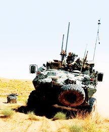
High-performance receiver manufacturers who design products for high-dynamic or high-vibration environments (see cover) where the contribution of phase noise from the local oscillator to velocity error cannot be ignored. In these areas, the strategy outlined here would produce equipment that can perform to higher specifications with the same or a lower-cost oscillator.
The trade-off requires two tracking channels per satellite signal, but this should not pose a problem. At ION GNSS 2009, manufacturers showed receivers with 226 tracking channels. There are currently only 75 live signals in the sky, including all of GPSL1/L2/L5 and GLONASS L1/L2. — Gérard Lachapelle
If the channel data within a GNSS receiver is handled in an effective manner, it is possible to form meaningful estimates of the local-oscillator phase deviations on timescales of 10 milliseconds (ms) or less. Moreover, if certain criteria are met, these estimates will be available with related uncertainties similar to the deviations produced by a typical oven-controlled crystal oscillator (OCXO). The processing delay required to form this estimate is limited to between 10 and 20 ms. In short, it becomes possible in near-real-time to remove the majority of the phase noise of a local oscillator that possesses short-term instability worse than an OCXO, using standalone GNSS. This represents both a new method to accurately determine the Allan deviation of a local oscillator at time scales previously impractical to assess using a conventional GNSS receiver, and the potential for the reduction in observable Doppler uncertainty at the output of the receiver, as well as ionospheric scintillation detection not reliant on an expensive local OCXO.
Concept. Inside a typical GNSS receiver, the estimate of the error in the local oscillator is formed as a component of the navigation solution, which is in turn based on the output of each satellite-tracking channel propagating its estimate of carrier and code measurements to a common future point. While this method of ensuring simultaneous measurements is necessary, it regrettably limits the resolution with which the noise of the local oscillator can be quantified, due to the scaling of non-simultaneous samples of local oscillator noise through the measurement propagation process. To bypass these shortcomings requires a method of coherently gathering information about the phase change in the local oscillator across all available satellite signals: to use the same samples simultaneously for all satellites in view to estimate the center-point phase error common across the visible constellation.
To explain how this is feasible, we must first understand the limitations imposed by the conventional receiver architecture, with respect to accurately estimating short-term oscillator behavior, and subsequently to determine the potential pitfalls of the proposed modifications, including processing delays needed for bit wipe-off, expected observation noise, and user dynamics effects.
Typical Receiver Shortfalls
In a typical receiver, while information about local time offset and local oscillator frequency bias may be recovered, information about phase noise in the local oscillator is distorted and discarded, as a consequence of scaling non-simultaneous observations to a common epoch.
As shown in FIGURE 1, coherent summation intervals in a receiver are used to approximate values of the phase error, including oscillator phase, measured at the non-simultaneous interval centrers in each channel, which are then propagated to a common navigation solution epoch. Each channel will intrinsically contain a partially overlapping midpoint estimate of oscillator noise over the coherent summation interval that will then be scaled by the process of extrapolation. As these estimates are scaled and partially overlapping, they do not make optimal use of the information known about the effects of the local oscillator, and form a poor basis for estimating the contributions of this device to the uncertainty in the channel measurements. As shown in Figure 1, the phase error measured in each channel will be distorted by an over unity scaling factor.
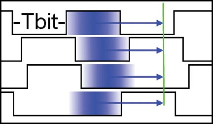
a typical receiver.
Depending on implementation decisions made by the designers of a given GNSS system, the average value of the propagation interval relative to the bit period will have different expected values. Assuming the destination epoch is the immediate end of the furthest advanced (most delayed) satellite bitstream, and that integration is carried out over full bit periods, the minimum propagation interval for this satellite would be ½-bit period.
For the average satellite however, the propagation delay would be this ½-bit period plus the mean skew between the furthest satellite and the bitstreams of other space vehicles. Ignoring further skew effects due to the clock errors within the satellites, which are typically limited well below the ms level, the skew between highest and lowest elevation GPS satellites for a user on the surface of earth would be approximately 10 ms. The average value of this skew due to ranging change over orbit, assuming an even distribution of satellites in the sky at different elevation angles, would therefore be 5 ms.
Combining the minimum value of the skew interval with the minimum propagation interval of the most delayed satellite yields a total average propagation interval of 15 ms. In turn, this gives a typical scaling factor of 1.75, used from this point forward when referring to the effects of scaling this quantity.
Proposed Implementation
Overcoming limitations of a typical receiver requires recording the approximate bit-timing and history of each tracked satellite as well as a short segment of past samples. This retained data guarantees that the bit-period boundaries of the satellites will not pose an obstacle to forming common N-ms coherent periods between all visible satellites, over which simultaneous integration may proceed by wiping off bit transitions. Using this approach as shown in FIGURE 2, all available constellation signal power is used to estimate a single parameter, namely the epoch-to-epoch phase change in the local oscillator.
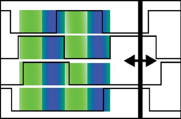
Having viewed the existence of these common periods, it becomes evident that it is conceptually possible to form time-synchronized estimates of the phase contribution of the common system oscillator alternately across one N-ms time slice, then the next, in turn forming an unb
roken time series of estimates of the phase change of the system oscillator. Forming the difference between the adjacent discriminator outputs will provide the following information:
- The ΔEps (change in the noise term in the local loop)
- The ΔOsc (change in the phase of the local oscillator, the parameter of interest)
- The ΔDyn (change in the untracked/residual of real and apparent dynamics of the local loop/estimator)
Noticing that term 1 may be considered entirely independent across independent PRNs (GPS, Galileo, Compass) or frequency channels (GLONASS), and that the value of term 3 over a 10-ms period is expected to be small over these short intervals, it becomes obvious that term 2 can be recovered from the available information. To determine the weighting for each satellite channel, the variance of the output of the discriminator is needed.
Performance Determination
To allow the realistic weighting of discriminator output deltas, it becomes desirable to estimate at very short time intervals the variance of the output of the phase discriminator. In the case of a 2-quadrant arctangent discriminator, this means one wishes to quantify the variance
![]()
Letting Q/I 5 Z, recall that if Y 5 aX then
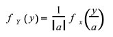
Applying this to the variance of the input to the arctangent discriminator in terms of the in phase and quadrature accumulators, this would give
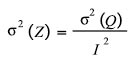
Rather than proceed with a direct evaluation from this point onward to determine the expression for the variance at the output of the discriminator, it is convenient to recognize that simpler alternatives exist since
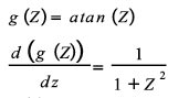
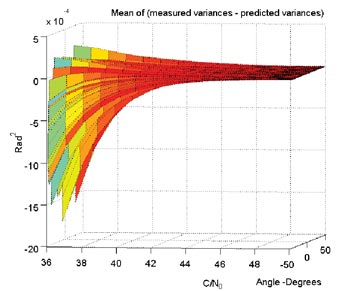
The implication is that since the slope of the arctangent transfer function is very nearly equal to 1 in the central, typical operating region, and universally less than 1 outside of this region, it is easy to recognize that the variance at the output of the arctangent discriminator is universally less than that at the input, and can be pessimistically quantified as the variance of the input, or σ2(Z). This assumption has been verified by simulation, its result shown in FIGURE 3, where the response has been shown after taking into account the effect of operating at a point anywhere in the range ±45 degrees. While the consequence of the simplification of the variance expression is an exaggeration of discriminator output variance, FIGURE 4 shows output variance is well bounded by the estimate, and within a small margin of error for strong signals.
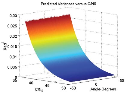
discriminator versus C/N0.
The gap between real and predicted output variance may also be narrowed in cases where Q>I by using a type of discriminator which interchanges Q and I in this case and adds an appropriate angular offset to the output as
![]()
Proceeding in this vein, the next required parameter is the normalized variance of the in-phase and quadrature arms.
The carrier amplitude A can be roughly approximated as
![]()
Resulting in a carrier power C

Further, the noise power is given as
![]()
Expressing bandwidth B as the inverse of the coherent integration time, and rearranging now gives noise density N0 as
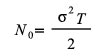
Combining this expression, and the one previously given for the carrier power C results in the following expression for the carrier to noise density ratio:
![]()
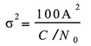
This latest expression can be rearranged to find the desired variance term. Assuming the 10-ms coherent integration time discussed earlier is used, this yields
Normalizing for the carrier amplitude gives the normalized variance in terms of radians squared:
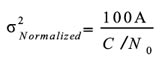
In any situation where the carrier is sufficiently strong to be tracked, it is likely that the carrier power term employed above can be gathered from the immediate I and Q values, ignoring the contribution of the noise term to its magnitude.
Oscillator Phase Effect. Determining the expected magnitude of the local oscillator phase deviation requires only three steps, assuming that certain criteria can be met. The first requirement is that the averaging times in question must be short relative to the duration, at which processes other than white phase and flicker phase modulation begin to dominate the noise characteristics of the oscillator. Typically the crossover point between the dominance of these processes and others is above 1 s in averaging interval length, when quartz oscillators are concerned. Since this article discusses a specific implementation interval of 10 ms within systems expected to be using quartz oscillators, it is reasonable to assume that this constraint will be met.
The second requirement is that the Allan deviation of the given system oscillator must be known for at least one averaging interval within the region of interest. Since the Allan deviation follows a linear slope of -1 with respect to averaging interval on a log-log scale within the white-phase noise region, this single value will allow an accurate prediction of the Allan deviation at any other point on the interval and, in turn, of the phase uncertainty at the 10 ms averaging interval level.
Letting σΔ(τ) represent the Allan deviation at a specific averaging interval, recall that this quantity is the midpoint average of the standard deviation of fractional frequency error over the averaging interval τ. Scaling this quantity by a frequency of interest results in the standard deviation of the absolute frequency error on the averaging interval:
![]()
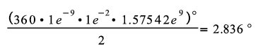
By integrating this average difference in frequency deviations over the coherent period of interest, one obtains a measure of the standard deviation in degrees, of a signal generated by this reference:
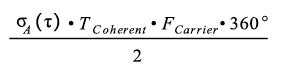
Note that the averaging interval τ must be identical to the coherent integration time.
Turning to a practical example, if the oscillator in question has a 1 s Allan Deviation of 1 part per hundred billion (1 in 1011), a stability value between that of an OCXO and microcomputer compensated crystal oscillator (MCXO) standard, and shown to be somewhat pessimistic, this would scale linearly to be 1e-9 at a 10-ms averaging interval, under the previous assumption that the oscillator uncertainty is dominated by the white phase-noise term at these intervals. Also, for illustration purposes, if one assumes the carrier of interest to be the nominal GPS L1 carrier, the uncertainty in the local carrier replica due to the local oscillator over a 10-ms coherent integration time becomes
When stated in a more readily digested format, this represents roughly 15 centimeter/second in the line-of-sight velocity uncertainty. In an operating receiver, two additional factors modify this effect. The first is the previously discussed scaling effect that will tend to exaggerate this effect by a typical factor of 1.75, as previously discussed. The second factor is that this noise contribution is filtered by the bandwidth-limiting effects of the local loop filter, producing a modification to the noise affecting velocity estimates, as well as reduced information about the behaviour of the local oscillator.
Impact of Apparent Dynamics. When considering the error sources within the system, it is important to realize which individual sources of error will contribute to estimation errors, and which will not. One area of potential concern would appear to be the errors in the satellite ephemerides, encompassing both the satellite-orbit trajectory misrepresentation and the satellite clock error. While the errors in the satellite ephemerides are of concern for point positioning, they are not of consequence to this application, as the apparent error introduced by a deviation of the true orbit from that expressed in the broadcast orbital parameters does not affect the tracking of that satellite at the loop level.
Additionally, while the satellite clock will add uncertainty to the epoch-to-epoch phase change within each channel independently, the magnitude of this change is minimal relative to the contribution of uncertainty due to the variance at the output of the discriminator guaranteed by the low carrier-to-noise density ratio of a received GNSS signal. Since this contribution is uncorrelated between satellites and relatively small compared to other noise contributions affecting these measurements, even when compared to the soon-to-be-discontinued Uragan GLONASS satellites that had generally less stable onboard clocks, it is likely safe to ignore. When compared to the more stable oscillators aboard GPS or GLONASS-M satellites, it is a reasonable assumption that this will be a dismissible contribution to received signal-phase uncertainty change.
While atmospheric effects present an obstacle which will directly affect the epoch-to-epoch output of the discriminators, it is believed that under conditions that do not include the effects of ionospheric scintillation the majority of the contribution of apparent dynamics due to atmospheric changes will have a power spectral density (PSD) heavily concentrated below a fraction of 1 Hz. The consequence of this concentration is that the tracking loops will remove the vast majority of this contribution, and that the difference operator that will be applied between adjacent phase measurements, as in the case of dynamics, will nullify the majority of the remaining influence.
Impact of Real Dynamics. Real dynamics present constraints on performance, as do any tracking loop transients. For example, a low-bandwidth loop-tracking dynamics will have long-lasting transients of a magnitude significant relative to levels of local oscillator noise. For this reason it is necessary to adopt a strategy of using the epoch-to-epoch change in the discriminator as the figure of interest, as opposed to the absolute error-value output at each epoch. This can reasonably be expected to remove the vast majority of the effects of dynamics of the user on the solution.
To validate this assumption under typical conditions calls for a short verification example. Assuming the use of a second-order phase-locked loop (PLL) for carrier tracking, with a 10-Hz loop bandwidth the effects of dynamics on the loop are given by these equations:
Letting Bn be 10 Hz, one can write
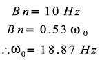
Recall that the dynamic tracking error in a second-order tracking loop is given by
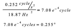
Given the choices above, this would result in a constant offset of 0.00281 cycles, or 1.011 degrees of constant tracking error due to dynamics, following from the relation between line-of-sight acceleration and loop bandwidth to tracking error. Since this constant bias will be eliminated by the difference operator discussed earlier, it is necessary to examine higher order dynamics.
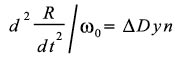
Further, if one used a coherent integration interval of 10 ms as assumed earlier, and let the dynamics of interest be a jerk of 1 g/s, this results in a midpoint average of 0.005 g on this interval:
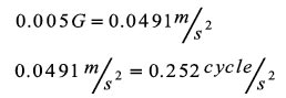
Substituting this result into equation 16 produces the associated change in dynamic error over the integration interval, which is in this case:
This value will be kept in mind when evaluating capabilities of the estimation approach to determine when it will be of consequence. As the estimation process will be run after a short delay, an existing estimate of platform dynamics could form the basis of a smoothing strategy to reduce this dynamic contribution further.
Estimated Capabilities
In the absence of the influence of any unmodeled effects, the expected performance of this method is dependent on only the number of satellite observables and their respective C/N0 ratios. Across each of these scenarios we assume for simplicity’s sake that each satellite in view is received at a common C/N0 ratio and over a common integration period of 10 ms.
If the assumption of minimal dynamic influences is met, the situation at hand becomes one in which multiple measures of a single quantity are present, each containing independent (due to CDMA or FDMA channel separation) noise influences with a nearly zero mean. When one can express the available data form:
x[n] = R + w[n]
where x[n] is the nth channel discriminator delta which includes the desired measure of the local oscillator delta (R), as well as w[n], a strong, nearly white-noise component, there are multiple approaches for the estimation of R.
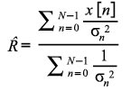
The straightforward solution to estimate R in this case is to use the predicted variances of each measure to serve as an inverse weighting to the contribution of each individual term, followed by normalization by the total variance, as expressed by
Now, since it is desired to bound the uncertainty of the estimate of R, the variance of this quantity should also be noted. This uncertainty can be determined as

To determine the performance of the estimation method for a given constellation configuration, with specific power levels and available carrier signals, it is necessary to utilize the predicted variances plotted in Figure 3 as inputs to equations 20 and 21. To provide numerical examples of the performance of this method, three scenarios span the expected range of performance.
Scenario 1 is intended to be char-acteristic of that visible to a single-freq-uency GPS user under slight attenuation. It is assumed that 12 single-frequency satellites are visible at a common C/N0 of 36 dB-Hz, yielding from the simulation curves a value for each channel of 0.0265 rad2. When substituted into equation 24, this predicts an estimation uncertainty of
![]()
This is a level of estimation uncertainty similar to that assumed to be intrinsic to the local oscillator in the previous section. The result implies that with this minimally powerful set of satellites, it becomes possible to quantify the behavior of the local oscillator with a level of uncertainty commensurate with the actual uncertainty in the oscillator over the 10 ms averaging interval.
Consequentially, this indicates that the Allan deviation of this system oscillator could be wholly evaluated under these conditions at any interval of 10 ms or longer. Further, if the system oscillator were in fact the less stable MCXO from the resource above, this estimate uncertainty would be significantly lower than the actual uncertainty intrinsic to the oscillator, providing an opportunity to “clean” the velocity measurements.
Scenario 2 is intended to be characteristic of a near future multi-constellation single-frequency receiver. It is assumed that eight satellites from three constellations are visible on a single frequency each, with a common C/N0 of 42 dB-Hz, yielding a value for each channel of 6.4e-3 rad2, leading to an estimation uncertainty of
![]()
Scenario 3 is intended to serve as an optimistic scenario involving a future multi-frequency, multi-constellation receiver. It is assumed that nine future satellites are available from each of three constellations, each with four independent carriers, all received at 45 dB-Hz, yielding a value for each channel of 3.2e-3 rad2, leading to an estimation uncertainty of
![]()
Application to Observations
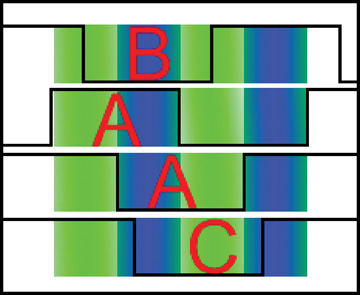
The theoretical benefit of subtracting these phase changes from the measurements of an individual loop prior to propagating that measurement to the common position solution epoch ranges from moderate to very high depending on the satellite timing skew relative to the solution point. The most beneficial scenario is total elimination of oscillator noise effects (within the uncertainty of the estimate), which is experienced in the special case (Case A, FIGURE 5), where the bit period of a given satellite falls entirely over two of the 10-ms subsections. The uncertainty would increase to 2x the level of uncertainty in the estimate in the special case (Case B) where the satellite bit period straddles one full 10-ms period and two 5-ms halves of adjacent periods, and would lie somewhere between 1 and 2 times the level of uncertainty for the general case where three subintervals are covered, yet the bit period is not centered (Case C).
While the application to observations of the predicted oscillator phase changes between integration intervals does not appear immediately useful for high-end receiver users with the exception of those in high-vibration or scintillation-detection applications, it could be applied to consumer-grade receivers to facilitate the use of inexpensive system clocks while providing observables with error levels as low as those provided by much more expensive receivers incorporating ovenized frequency references.
Further Points
While the chosen coherent integration period may be lengthened to increase the certainty of the measurement from a noise averaging perspective, this modification risks degrading the usefulness of said measurement due to dynamics sensitivities. Additionally, as the coherent integration time is increased, the granularity with which the pre-propagation oscillator contribution may be removed from an individual loop will be reduced. While this may be useful in cases of very low dynamics where the system is intended to estimate phase errors in a local oscillator with high certainty, it would be of little use if one desires to provide low-noise observables at the output.
For this reason, it is recommended that increases in coherent integration time be approached with caution, and extra thought be given to use of dynamics estimation techniques such as smoothing, via use of the subsequent n-ms segment in the formation of the estimate of dynamics for the “current” segment. This carries the penalty of increased processing latency, but could greatly reduce dynamics effects by enabling their more reliable excision from the desired phase-delta measurements.
Acknowledgments
The author thanks his supervisors, Gerard Lachapelle and Elizabeth Cannon, and the Natural Sciences and Engineering Research Council of Canada, the Alberta Informatics Circle of Research Excellence, the Canadian Northern Studies Trust, the Association of Canadian Universities for Northern Studies, and Environment Canada for financial and logistical support.


