Take a look at the major manufacturers of multi-frequency GNSS equipment and the markets they serve. Obviously, surveying is an important market; construction is a major one too. Maybe you’ve noticed that agriculture is also making its way up the food chain, so to speak. Trimble, Topcon, Leica/Novatel, Deere/Navcomm, and Hemisphere GPS are all pursuing the precision agricultural market with RTK-like precision.
The terms “precision agriculture” and “precision farming” have been around for a long time. There are conferences dedicated solely to sharing information on this topic, such as the 9th International Conference on Precision Agriculture. The classic precision ag market has been relatively unchanged for the past decade or so. Yes, in the past few years WAAS (Wide Area Augmentation System) has made a substantial impact with respect to a reliable and convenient source of corrections for one-meter accuracy using GPS, but all in all, one-meter accuracy is what most precision ag users have adapted to.
Stepping back, GPS/GNSS is only one component of the precision agriculture puzzle. Remote sensing (aerial photography/LIDAR), various sensors, and GIS (geographic information systems) software all play a key role in enabling people to record, analyze, and apply data used to make decisions that optimize the output of a particular agricultural area.
There are a few keys areas where GPS/GNSS is used in agriculture, though. These aren’t all-inclusive, but cover significant tasks where GPS has been very beneficial.
Field mapping: there have always been field maps of some sort, whether they were hand-sketched or derived from an aerial photo, but GPS has improved the precision substantially. Not only can one map the perimeter of the field, but also infrastructure such as roads, drain tile, outlets, wells, buildings, etc. The farmer doesn’t necessarily do this, but fertilizer distributors have become GPS-savvy and offer this service.
Yield mapping: as crops are harvested, a GPS receiver connected to a yield monitor sensor records a coordinate along with the yield data. This data is combined and analyzed to create a map of how well different areas of the field are producing.
Guidance: when spreading fertilizer or planting, equipment operators have traditionally used markers such as foam or other visual aids to mark where they’ve been to try and avoid overlap. The assistance of GPS and onboard guidance systems, such as a light bar, can further reduce overlap.
As I mentioned before, for many years precision ag users have settled for one-meter precision. Companies like Hemisphere GPS (formerly CSI Wireless) did very well designing single-frequency GPS receivers for the precision ag market. Hemisphere is also a leading designer of radio beacon (Coast Guard) receivers. Radio beacons, in addition to WAAS, are a free source of corrections for one-meter accuracy. Trimble was also an early supplier of precision ag GPS receivers and related equipment, typically offering single-frequency products like the AG-132.
While the real-time kinematic (RTK) technique has been around since the early 90s, it didn’t gain wide acceptance in the precision ag industry. The accuracy was great, down to approximately 2 cm at the time, but the equipment was clunky. The user had to set up a reference station near the field he was working on. The communication link was complicated, and some types needed Federal Communications Commission (FCC) licensing. Consequently, there were several potential points of failure. Lastly, the cost for a complete RTK system (base, rover, and radios) was high, upwards of $50,000. It just wasn’t cost-effective.
What is an RTK Network?
It’s an ambiguous term, because it means different things depending on the industry, but essentially the hardware setup is the same no matter which industry we are discussing. An RTK network is a series of dual-frequency reference stations spaced optimally within a region so as to provide RTK corrections to subscribers within that region. Following is an illustration of an RTK network for agriculture in the Ohio area.
All the reference stations are surveyed (more on that below) with respect to one another.
The network subscriber is assigned a primary reference station to use. RTK networks for agriculture are single-baseline solutions; the subscriber can only use one reference station at a time. There is no “network solution” per se, or redundancy like there is in RTK networks used in the surveying and construction industries. Therefore, when a single reference station “goes down,” the subscribers in that area are down also. There is software available from RTK network vendors that allows the administrator to monitor all reference stations via the Internet, but some networks don’t have that feature implemented. In that case the administrator hears about problems when subscribers have problems.
Another major difference between RTK networks for agriculture and RTK networks for surveying and construction is the communication method. The latter primarily use data plans on mobile phones to receive corrections. Either the mobile phone is linked via Bluetooth to the receiver or a cellular modem is built inside the receiver.
RTK networks for agriculture, on the other hand, primarily use spread spectrum radios (900 Mhz band) to transmit corrections to the receiver. The benefit of a spread spectrum radio is that they are free to use and don’t require a license from the FCC to operate. They are limited in their broadcast range, however, which is typically two to three miles. To solve this problem, radio repeaters are used to extend the distance. Depending on the topography, as many as four repeaters may need to be permanently mounted to effectively cover the broadcast range needed, based on the spacing of the reference stations. Even then, there may still be some areas that are not fully covered. In that case, temporary mobile repeaters may be used to provide coverage to that area.
The Wild, Wild West of RTK Networks
Bill Henning, real-time specialist with the National Geodetic Survey (NGS), said it best: the recent explosion of RTK networks is like the Wild, Wild West. They are proliferating so quickly that it’s hard to keep track of them. One of his tasks is to help develop guidelines for RTK network operators, and I think NGS is making inroads into the survey/construction industry with their initiative. People are looking for that sort of guidance with respect to RTK network setup, as well as monitoring for the networks once they become operational.
RTK networks for agriculture seem less structured than in other disciplines, though, and administrators rely more heavily on vendor recommendations. For example, some are based on the ITRF reference frame, while others are based on some version of NAD83. Some networks hire land surveyors to establish their reference station locations, while others do it themselves using NGS’s OPUS program or other methods. Very few, I think, realize the resources available from the NGS, such as the Cooperative CORS program.
Separate Industries, Separate RTK Networks
Even this early in the RTK network game, the duplicity of networks between agriculture and survey/construction is interesting. For example, an RTK network for agriculture can cover the same area as an RTK network for survey/construction. In the state of Georgia, there are several RTK networks for agriculture and several for survey/construction, some of which overlap. In fact, one would think that these folks (ag and survey/construction) would consolidate their efforts. The RTK network equipment is virtually the same. But alas, the manufacturers don’t want this. Why not? To answer that question, just employ the old adage: follow the money.
The fact is that a farmer isn’t going to pay the same RTK network subscription rate that a surveyor or construction company will. The numbers are vastly different. The typical subscription rate for access to an agricultural RTK Network is $1,300 to $1,500 per unit per year. Subscription rates for access to a survey/construction RTK network are as high as $4,500 per unit per year.
Some industry folks say that aggressive subscription pricing is the reason RTK networks in the agriculture market have expanded rapidly in the past few years. A farm is very hesitant to pay $4,500 annually when they can select a service like OmniSTAR and pay $1,500 annually.
Again, there are differences between the networks used in agriculture and those in survey/construction; most, if not all, are software-related. RTK networks for survey/construction offer a true networked solution, where several reference stations are used to compute a correction, whereas RTK networks for ag are single-baseline solutions, like users would normally set up as a base rover for their own use.
Others at the Party
Of course, OmniSTAR (HP/XP),Deere (Starfire), and Novariant (AutoFarm) offer a GPS-based solution in the precision ag industry. They are not pure-play RTK solutions like RTK networks are, although they do have RTK capability. True RTK networks are capable of constantly delivering ~2 cm accuracy day-in and day-out. These folks going after the precision ag market offer decimeter-level services primarily (1 decimeter being the equivalent of 10 cm), and then RTK solutions when needed.
It will be interesting to see how pure-play RTK players respond as RTK networks for agriculture continue to expand … which they most certainly will.
While European regulatory authorities are closely scrutinizing the proposed TomTom/Tele Atlas merger, they have also turned their eyes to the proposed Navteq/Nokia deal.
Navteq Corp. said today that the European Commission has initiated a second-phase review of Nokia’s pending acquisition of Navteq. The company stressed in its announcement that this is part of the commission’s review process and does not signal the ultimate outcome. Nevertheless, it is a rare, if not extraordinary step for the commission; in the past 10 years it has only initiated a second-phase review in about 3 percent of European mergers of publicly held companies.
The Commission now has 90 working days to make a final decision on the transaction. However, the review period may be extended to 125 working days. Such has been the case with the TomTom/Tele Atlas deal, also under a second-phase review. Those two companies are anticipating a commission decision on their merger by May 21.
Both Navteq and Nokia said they remain committed to their merger plans, noting that the deal has received all the other necessary regulatory approvals, including anti-trust approval in the United States.
Meanwhile, TomTom said March 27 that it was extending the period of its offer for Tele Atlas. It was clear the European Commission wouldn’t reach a decision by the end of the previous time frame attached to the offer to acquire Tele Atlas for €30 per share, or about €2.9 billion, which would have ended March 31, TomTom said. As result, it has extended its offer to May 30. The Commission originally announced that it was initiating a second-phase review of the merger in November of last year.
Global Trek Xploration, a provider of embedded miniaturized GPS technologies, has completed a share exchange transaction merger with Deeas Resources Inc.
In conjunction with the transaction, the combined public entity is operating as GTX Corp. Global Trek Xploration is now wholly owned by GTX Corp, a publicly-held company, with shares quoted on the Over-The-Counter Bulletin Board (OTCBB : GTXO.OB). Patrick Bertagna, founder, current CEO, chairman of the board, and president of Global Trek Xploration, assumed those same duties for GTX Corp. while Jeffrey Sharpe, CEO and president of Deeas Resources Inc., joined GTX Corp’s board.
“The next logical step was for us to become a publicly traded company,” Bertagna said. “The influx of new capital gives us the ability to launch our unique, miniaturized GPS technologies on to the global stage. We look forward to continuing the momentum we have achieved and sharing our successes with our shareholders.”
Concurrent with the share exchange, GTX Corp. also completed an equity financing through a private placement of its common stock and stock purchase warrants for an aggregate amount of $8 million. The proceeds from the first tranche of financing will support the continued development of its miniaturized GPS real-time tracking technology and the licensing of its gpVector technology to branded consumer product partners.
I covered this subject a while back, but I think it’s time to revisit it. Personal navigation devices (PNDs) are still selling like crazy. If you don’t have one, someone you know does. Tens of millions of these things are being sold per year.
If you don’t have one yet, you’ve got some options, because you can take it as a tax deduction. Perhaps a bit of “consult your accountant” verbiage should go here, but any time you need to drive from Point A to Point B for your job, I think you can take it as a deduction. Even if you do pay full price, it’s still a bargain.
First of all, you must be aware of the explosion in the number of consumer navigation units recently — you know, the Garmins, TomToms, Magellans, Mios, and Navigons of the world. If you go to Best Buy, Fry’s, Circuit City — even Radio Shack — you’ll see a bazillion of them on the shelf.
Disregarding the personal benefits of having one, I think they are one of the biggest bangs for your buck today, in terms of job efficiency. With labor being so expensive, I don’t see how a company can afford not to have one of these in each rig that’s headed to a job site. How many times have you (or one of your crew) gotten lost trying to find a job site, the local Home Depot, an ATM, or whatever? You aren’t just wasting your own time by being lost; it has a ripple effect.
I agree that PNDs aren’t for everyone. The solo surveyor working in his or her hometown and immediate surrounding towns probably knows the area better than Rand McNally. I’m thinking more along the lines of a contractor (be it a survey company or whatever) that has multiple people going in and out of a project. Maybe some employees are commuting directly from their homes, some are coming from the office, etc.
I think it’s hard to measure the stress, time spent, and other impacts of figuring out directions when working in an area that is not well known to the driver. Ever since I started carrying a little GPS navigator with me, I’ve virtually stopped using MapQuest or worrying about dealing with directions of any sort. Maybe you’re not like me, where you want to have all directions planned out in advance so you can stick to a tight schedule. To accomplish that, part of my preparation once included printing out all the directions and maps from MapQuest. I don’t bother with any of that now.
Even if you don’t use the directions feature, you’ve got a complete, nationwide electronic map at your fingertips. You can zoom out, zoom in, and pan around the screen. Following are some sample screens:
Which One Is Best?
Well, it depends. I hate that answer when I hear it, but it’s true. But this shouldn’t lead to “analysis paralysis,” where you can’t decide what to do so you don’t do anything. For me, there are four general features that are important to consider, no matter which additional bells and whistles you desire:
Display size. There is nothing worse than having to squint and try to focus on a micro-map when you are supposed to be driving. I like a large (relatively speaking), bright display. There are a couple of very common display sizes: 3.5-inch and 4.3-inch. Of course, the larger the display is, the larger the overall unit size is (and usually, the more expensive). I think the tradeoff is worth it for the larger screen size.
Ruggedness and reliability. It’s no better than a rock on your dashboard if it doesn’t work. I hate the flip-up antennas. Not many of the newer units have those any longer, but some of the older ones do. They are begging to get snapped off, unless you leave them permanently mounted on your dash. Also, some of the windshield mounts are pretty hokey, so be aware. In general, the various cable connections should appear solid.
Battery life. I guess this one depends on how you are going to use it. Personally, I like to take it from my dash and throw it in my laptop bag when I’m traveling by air. I dislike battery chargers in general (a necessary evil in this business), so I prefer a unit that will operate for at least five hours on one charge so I don’t have to cart the charger around with me.
Spoken street names. This is called “text-to-speech.” You can live without it, but it’s a nice feature. Instead of telling you “turn right in 500 feet,” it says “turn right in 500 feet on Main Street.” The lower-priced models typically don’t have this option.
There are many, many other bells and whistles you might like, such as real-time traffic data, Bluetooth for hands-free phone use, MP3 players, an FM interface to your vehicle sound system, etc., but those are more a matter of personal preference.
As coordinate-centric people, a lot of surveyors and mappers like to use State Plane. Very few navigation units support this sort of feature, although some support loading USGS topo maps in the background. I’m of the mindset that you really don’t want to try to do too many things with a PND, though. Call it a navigator and let it go at that. If you want a more coordinate-centric unit, then you’ll have to buy something other than a PND, like a Garmin GPSMAP 60CSx, DeLorme PN-20, or Magellan Triton.
I’ve put together a partial list of units with different features. The links are generally to the manufacturers’ websites, so don’t use the prices listed there as a reference.
3.5″ Display Units
TomTom ONE 3rd Edition (2-hr battery life, no text-to-speech, street-priced under $200).
Garmin Nuvi 200 (up to 5-hr battery life, no text-to-speech, street-priced under $200).
Garmin Nuvi 260 (up to 5-hr battery life, text-to-speech, street-priced under $300).
Magellan RoadMate 1200 (2-hr battery life, no text-to-speech, street-priced under $200).
Magellan CrossoverGPS (8-hr battery life, text-to-speech, IPX-4 waterproof rating, can load USGS topos, street-priced under $300).
Mio C220 (4-hr battery life, no text-to-speech, street-priced under $200).
Mio C310x (4.5-hr battery life, text-to-speech, street-priced under $250).
4.3″ Display Units
TomTom ONE XL (2-hr battery life, no text-to-speech, street-priced around $200).
TomTom GO 920 (up to 5-hr battery life, text-to-speech, street-priced under $500).
Garmin Nuvi 200W (up to 5-hr battery life, no text-to-speech, street-priced under $200).
Garmin Nuvi 880 (up to 4-hr battery life, text-to-speech, street-priced under $1,000).
Magellan Maestro 4200 (up to 4-hr battery life, text-to-speech, street-priced under $400).
Magellan Maestro 4250 (up to 4-hr battery life, text-to-speech, street-priced under $500).
Mio C320 (4-hr battery life, no text-to-speech, street-priced under $200).
Mio C720t (up to 3-hr battery life, text-to-speech, street-priced under $400).
There are many other navigator units on the shelves at the store. I’ve just listed ones from the top four market leaders.
You’ll notice I didn’t mention anything about the software interface. There are many opinions floating around about Brand X interface being better than Brand Y. After using a lot of different PNDs, I think the argument is about the same as Brand X total station/GPS vs. Brand Y total station/GPS. Most have very similar functionality, and their own idiosyncrasies, so it’s just a matter of getting used to it. One thing is for sure: the user interfaces are all different.
Don’t be stymied by analysis paralysis. A PND is the sort of tool (or toy) that once you get used to it, you can’t imagine working without it. Remember when folks fought against the electronic data collector, back when it was first introduced?
Several weeks ago, I attended the ESRI Federal User Conference, held February 20-22 in Washington, D.C. I wish I could report on some earthshaking new technology that is going to change everything, but as with most mature technologies, what I saw were mostly refinements of existing technologies such as ArcGIS 9.3.
In 9.3, scheduled to ship in June, Web connectivity and integration have been improved, as have 3D tools and applications. An automatic Send Crash Report to ESRI notification has been added, along with very easy integration and connectivity with Google and Microsoft. Other improvements include working under the Vista operating system and enhancements to Model Builder.
I’ve been a strong advocate of Spatial Analyst and its use with Model Builder, which has greatly simplified this aspect of GIS. Too many GIS users have been stuck in a “point, line, and polygon” GIS, but not all GIS data have discrete borders. Most environmental and social data have fuzzy boundaries and can only be modeled accurately as continuous functions. The beauty of Spatial Analyst (GRID) is that if you can mathematically describe what is happening, Spatial Analyst can model and display the phenomenon.
I know that grid cell modeling can get difficult, but the grid cell environment is a powerful tool that can take some GIS projects to the next level of accuracy and completeness. Grid cell modeling is also significantly faster than trying to force polygons into a large dynamic model.
I did see one new dataset that could be very valuable to certain users: Robert Renner of the U.S. Department of Housing and Urban Development demonstrated a free dataset from the U.S. Postal Service on address vacancies. It can be used to identify neighborhood changes showing emigration (vacated homes) or new neighborhoods (not-yet-occupied homes). This dataset is an early indicator that could be very useful for economic development, crime prevention, and public safety applications.
Although most attendees didn’t observe any major developments in GIS, it was a good opportunity to network and see what peers in other agencies are doing. Over years of attending conferences, I’ve found that unless you’re new to the business, 95 percent of the information presented is old news. What makes the events worthwhile is discovering that little gem, that new piece of information or technology that you would have missed otherwise.
It’s tough putting on a conference for such a diverse group of attendees, whose interests and experience levels run the gamut. With that in mind, and remembering the story of the blind men describing an elephant, I asked several of my fellow attendees what gems they uncovered at the 2008 FedUC.
William Gray and Tony Ferguson of the National Geospatial-Intelligence Agency are long-term users of GIS, and neither saw much that was new other than the refinements shown in ArcGIS 9.3. On the flip side, Beth Dorch and B. Schumacher of the FBI got great benefit from some entry-level sessions, such as GIS basics and GIS definitions. They also touted the value of a simple, yet real-world demonstration of how ArcGIS was used for law enforcement analysis.
Jim Mars of the Army Corps of Engineers liked the workshop demonstrating Model Builder, which showed how he could use the information for state shelters. Annette Miller, Montana Department of Labor, was new to GIS, so everything in the expo and all the sessions was new information and a major revelation.
Brian Sterling, U.S. Department of Agriculture, Maryland, learned more about ArcExplorer and was happy to find out about TerraGo’s GeoPDF format — especially the publishing and collaboration tools. Craig Oaks of ProLogic appreciated being able to form a big picture of how customers are using GIS and how ProLogic fits in.
An unscheduled — but valuable — session was presented by Anne Miglarese, who is leading the effort to establish the National Geospatial Advisory Committee. This is a newly formed group composed of key public and private geospatial professionals that will use the public-private partnership to advance GIS and promote data sharing. This could provide a much-needed shot in the arm for the National Spatial Data Infrastructure.
Miglarese explained the genesis of the committee, and highlighted the fact that all meetings will be open to the public, and the material discussed will be available through a Web site that all can access. I know several members of this committee, and I believe it will have a significant and positive impact on GIS and geospatial efforts.
The closing session was a very interesting presentation by David Kinley of SPAWAR. David explained how NORTHCOM and the Department of Homeland Security (DHS) had learned lessons from Katrina response and created interoperable systems to respond quickly to natural and manmade disasters, civil disturbances, and special events such as pending political conventions. NORTHCOM and NORAD use a system called SAGE, while DHS uses a system called iCAV. He also discussed TRITON, a Web-based critical infrastructure protection system used by the Army Corps of Engineers.
Through a combined effort, data stovepipes were eliminated, and data sharing is now the norm. David addressed the difficulty in finding trained and qualified people to support these systems and noted that the agency is turning to the service academies to train new personnel.
I found the last 30 minutes to be the most interesting part of the conference. Jack Dangermond announced that by popular request, ESRI was going to establish an Intel User Community that will be facilitated by Mark Schultz, ESRI’s director of intelligence. Jack then had an open-mic question-and-answer session with the audience. Unlike the current array of politicians, he didn’t have pre-screened and pre-approved questions. Some of the questions were very penetrating, and I almost cringed for him when I heard some of them. But he answered all the questions with great candor.
Jack has built a worldwide organization that almost has a cult following. One only needs to experience the annual User Conference, attended by 13,000, to get a sense of that culture. From a federal perspective ESRI, ArcGIS, and all the related software programs have become a critical national resource. GIS is now fully integrated in all aspects of federal operations, as shown by this year’s speaker and attendee list. So people are understandably curious to see how developments at Google and Microsoft are affecting GIS.
One member of the audience asked Jack why Google and Microsoft seem to be building such strength in GIS-related efforts such as Google Earth and Microsoft Virtual Earth, whether this poses a threat to ESRI, and why ESRI didn’t dominate this area. The ESRI president answered in a way that only someone who is really confident in his work and organization can.
He replied that the goals and funding of ESRI, Google, and Microsoft are directed toward different purposes. ESRI is a company whose resources of roughly 600 million dollars per year are reinvested to expand the body of GIS knowledge, further the use of GIS, and support GIS customers. Google and Microsoft have billions to devote to the key goal of driving customers to advertisers. They are interested in search engines, base maps, and mapping to capture 8 to 10 billion dollars in ad revenue, not the smaller technical niche of GIS. On the other hand they could decide to take over GIS and then we’d be out of business, Jack said with a wink.
One last question dealt with concerns about the openness of our society and the accessibility of information by terrorists, especially GIS data. Jack indicated that this also concerned him, but he was comforted by the thought shown by history that open societies ultimately are more successful than closed ones. On that note, the conference concluded.
After the conference I was able to talk with Jack, and I shared with him common feelings and conclusions I’ve heard from many first responders, planners, and DHS personnel regarding access to data. Most believe that it would be impossible to get the information genie back in the bottle. Additionally, determined terrorists can get information they need even without high-tech tools because they have the advantage of choosing and researching a specific target, even with simple ground-level photos and personal observations.
First responders, however, must be in a position to respond quickly and effectively to all possible targets, since they don’t have the advantage of knowing a target ahead of time. That tips the scale in favor of having accurate and complete datasets and imagery readily available for our first responders. Jack was comforted by that information, and indicated that he would use it in other discussions. I would appreciate hearing from anyone with a different point of view who would like to share the reasoning behind it; please contact me.
Overall, it was a good conference that met the needs of a very diverse group of attendees. I believe that everyone who attended came away with at least one new piece of information or insight that made the conference worthwhile.
There has been a lot of activity on both the civilian and military sides of GPS/GNSS these past few weeks. Instead of a central theme to this newsletter, I’m going to comment on three points of interest: a DoD directive regarding position, navigation, and timing; PRN32; and some new product developments.
New Department of Defense Directive
On February 19, 2008, the Deputy Secretary of the U.S. Department of Defense (DoD) issued Directive #4650.05, which addresses, among other things, the “policy, procedures and responsibilities” for GPS. Although there will be many who will dissect and analyze the Directive for weeks to come, it’s clear that civilian influence on GPS continues to rise. You can read our Military and Government Editor Don Jewell’s initial comments here.
Of interest to the survey/construction/mapping community is the fact that the Department of Transportation is specifically mentioned as a key external agency (external to the DoD) to have a say in GPS activities. The Department of Homeland Security and NATO were the other two key external agencies named.
There is nothing earth-shattering about the directive, but it certainly sends a strong message that the federal government wants the civilian community — domestic and perhaps more so, international — to feel more comfortable about GPS, even though it’s still a U.S. military program.
PRN32
After a few months of waffling and discussion and announcements, PRN32 was finally set healthy. It’s been ready to go, but there has been concern about the effect that it would have on GPS receiver firmware. It was suspected that some GPS receivers wouldn’t be able to handle it, or would be adversely affected by it, because they may interpret PRN32 as PRN00.
This isn’t the first time that DoD has used PRN32. PRN32 was used temporarily in the early 90s until it was discovered that some GPS receivers interpreted it as PRN 00. It hasn’t been used again until now, some 15 years later.
Chances are that your receiver should be able to handle PRN32, given the event back in the early 90s and the DoD memo released more than a year ago. The satellite in question was set healthy on February 26, 2008. If your receiver is tracking but still not using PRN32, it may be worth a call to the dealer or manufacturer of your equipment to see if there is a firmware update available.
Depending on your location, PRN32 may help you. I was in the field in the western United States a couple of weeks ago, for example (before PRN32 was set healthy). I was only using five GPS satellites with an RTK receiver while down in a hole, and my receiver was tracking PRN32. It was in a perfect part of the sky that would’ve probably allowed me to get the tough shot I wanted, had it been set to healthy at that time, but no dice. I’m going back to the same site in a few weeks, and I’ll be watching for it. The RTK receiver I was using is more than 10 years old, so it will be interesting to see how it handles a healthy PRN32.
Product Announcements
Normally, I leave the new product announcements out of the editorial area, but three recent ones deserve particular attention. I mentioned two of them, from Javad GNSS and Magellan, in my December column of who to look out for in 2008. Both companies have come through in short order.
Javad GNSS. Early last month, Dr. Javad Ashjaee — former Trimble engineer and founder of Ashtech, Javad Positioning Systems (which was sold to Topcon in 2000), and Javad Navigation Systems — introduced the world to products developed by his new venture: Javad GNSS. In true Javad style, he’s pushing the envelope on both the technical side and the business side of the equation.
Of course, it’s expected that Javad’s new product line would account for every signal available, and probably every one that is planned. No disappointment there. His Triumph technology sports 216 channels to track everything from GPS L1/L2/L5 to Europe’s E1/E5 Galileo to GLONASS L1/L2, as well as all SBAS signals. That’s no big news, though, as all the other major manufacturers offer similar products.
What’s new and unique about Javad’s offering is the “RTK Umbrella.” The concept makes sense. The idea behind the RTK Umbrella is to increase the reliability of RTK positioning. A cluster of four antennas (on the rover) is used to compute sixteen baselines for every RTK measurement. Here is what the umbrella looks like.
After looking at it, you’re probably thinking the same thing I am: How am I going to cart that thing around all day? The short answer is, you won’t. But I can see an application where one could use the RTK Umbrella for setting control and performing other geodetic functions that require a higher degree of reliability and integrity. Then, you could toss it into the back of the truck and just use the single antenna for the production work.
It’s an interesting concept. I’ve got to give the guy credit for being creative.
Magellan. Magellan has been noticeably quiet in the high-end, survey-grade survey business for quite a while. The roots of their high-end business came from Ashtech, which they acquired many years ago. Yes, they have the Z-Max.Net that they announced a couple of years ago, but in a world where multi-constellation GPS and GLONASS receivers are the norm, it’s a me-too product at best. To give credit where credit is due, Magellan has continued to dominate the lower-end L1 survey-grade receiver market with its ProMark series of receivers and more recently, its ProMark 3 RTK product.
Now, as the company has been threatening to do (albeit under its breath), it has placed both feet squarely back in the high-end survey receiver business with the ProMark 500, a multi-constellation receiver that places Magellan in the same class as the best Trimble, Topcon, and Leica receivers. Granted, there is not a lot of information available on the ProMark 500, other than the video on its website. The real test will be when Magellan starts to ship the product, and dealers and users begin to run it in production mode.
My guess is that the technology will be pretty good. I think one of the biggest challenges will be to rebuild their surveying distributor network. With Topcon and Leica buying up distributors like candy in the past twelve months, the pickin’s are getting pretty slim.
Trimble. Remember when the Trimble ProXRS was the cream of the sub-meter mapping crop of receivers? It was a L1 C/A code workhorse of the past decade around the world. Then, it faded away when the ProXT/ProXH receivers were introduced. But neither of those really replaced the ProXRS.
Now, Trimble has upped the ante by introducing the ProXRT. The ProXRT offers users a range of accuracy depending on their needs, from sub-meter down to decimeter (10cm) accuracy. Perhaps the most significant feature is that the ProXRT is capable of using the Russian GLONASS satellites as well as GPS. The product announcement implies that GLONASS signals are used when GPS satellite availability is impaired. I have two comments about GLONASS on mapping-grade receivers.
Unless you are using your own GPS/GLONASS reference station, the GLONASS signals used on a mapping-grade handheld will be uncorrected (autonomous). Virtually no CORS receivers have GLONASS capability; neither NDGPS nor WAAS/EGNOS use GLONASS. So, there are no free public correction sources for GLONASS like those we are used to with GPS. However, many RTK networks are broadcasting both GPS and GLONASS corrections.
Autonomous GLONASS measurements offer much worse accuracy than autonomous GPS measurements, by a factor of five. This is because of the inferior clock and ephemeris data.
However, if used in the right circumstances, tracking a GLONASS satellite(s) can be the difference between getting a measurement or no measurement at all — even if the accuracy of the position takes a hit.
Another feature that the ProXRT brings back, which was curiously missing from the ProXT and ProXH, is OmniSTAR capability. The ProXRT is capable of using OmniSTAR’s VBS, XP, or HP service. This, of course, means that the ProXRT is a GPS L1/L2 receiver.
I’ll be attending the annual ACSM Conference on Thursday of this week. I’ll keep my eyes open for any other new developments. I’ll probably blog or otherwise comment on the conference somewhere on the GPS World website, as that is becoming our modus operandi when attending conferences. I like that format, and it brings you a bit closer to what’s happening if you are unable to attend the conference yourself.
By VASILIY ENGELSBERG, IVAN PETROVSKI, and VALERY BABAKOV
Similar in many aspects to GPS, GLONASS has performed much less successfully on a commercial scale, failing — so far — to create significant business worldwide. Today, however, the commercialization of GLONASS has taken a new and more promising direction, receiving strong encouragement from the Russian government. We look forward to GLONASS being completely restored to its full operational capabilities within the next few years, and we are certain that this time GLONASS will create successful business opportunities worldwide.
Why did GLONASS fail to create a worldwide business opportunity in the past? First, many GLONASS satellites of the first generation had required replacement at approximately the same time. This coincided with a difficult period for the Russian economy, after the collapse of the Soviet Union and much of its infrastructure. Budget for space applications suffered, not only for GLONASS, but other space programs that were temporarily frozen. Many companies that had started to work on combined GPS/GLONASS receivers worldwide stopped these initiatives at that time.
The other reason for GLONASS’s halting commercial history is in its frequency division multiple access (FDMA) signal structure instead of code division multiple access (CDMA), as is the case with GPS, and now Galileo. FDMA, though more immune to interference, results in bulkier user equipment. Today the situation may change in two respects. First, there is a possibility of introducing CDMA within GLONASS. Second, and even more important, today GNSS user equipment progresses toward multifrequency anyway with all the possible combinations of GPS, Galileo, L1, L2, and L5. It will ultimately boost the technology, and even multifrequency and wide-band RF components will be miniaturized.
All these considerations allow us to confidently foresee exceptional opportunities for GLONASS-related business tomorrow.
Policy. Today, GLONASS is required for social infrastructure within Russia for all federal users. President Vladimir Putin has paid special attention to rapid GLONASS development, urging completion of the system ahead of the original plan.
As expected, three more GLONASS-M satellites were launched by the end of 2007, and have since been declared operational. GLONASS-M satellites have a guaranteed lifespan of seven years, that is, the lifespan of these satellites runs until the year 2015.
There is also a new generation of satellites, GLONASS-K. This upcoming modification represents an entirely new concept based on a non-pressurized platform. The estimated service life of GLONASS-K satellites has been increased to 10–12 years, and the spacecraft will carry an additional third civilian L-range frequency.
GLONASS-K is smaller and considerably lighter than previous models, allowing the use of a wider range of launch vehicles and thus making them less costly to put into orbit. The weight of a GLONASS-K satellite falls to 700 kilograms instead the of 1,415 kilos of previous satellites. After the complete constellation is deployed, it will require one Soyuz launch per year to maintain the constellation in full.
We expect that at least six GLONASS-M satellites will be launched in 2008, and six more in 2009. There will also be two GLONASS-K satellites launched in 2009. The earlier satellites with three-year lifespans will be decommissioned.
Altogether, there should be 24 satellites in near-circular orbits with 64.8-degree inclination in three orbital planes. Initially, system completion was planned by the year 2012, but with close attention from the Russian government, the system may be deployed in full scale by the end of 2009.
Interoperability. Moving as planned toward interoperability with GPS and future Galileo, the GLONASS coordinate frame had been changed. According to the Russian Federation government decree issued on June 20, 2007, the improved version of the national geocentric coordinate system “Earth Parameters 1990” (PZ-90.02) has been applied to GLONASS. The transformation between PZ-90.02 and the International Terrestrial Reference Frame ITRF2000 contains only origin shifts along X, Y, Z by –36, +8, and +18 centimeters, respectively. An update to the GLONASS Interface Control Document has already been published and made available trough the Internet. The update to ICD, current information on GLONASS status, and a current almanac is available from the Information-Analytical Center (IAC).
Worldwide Use
All restrictions on positioning service in Russia were lifted in January 2007, including a restriction on allowed positioning accuracy. This was one of the barriers that limited GLONASS commercialization in the past.
Today, GLONASS plus GPS user equipment appears more and more frequently in stores in Russia. It is now necessary and highly popular equipment for airplanes, marine applications, surveyors, mapping applications, and so on.
What advantages does GLONASS offer to worldwide users who already have GPS? Due to its orbit inclination, GLONASS provides better coverage than GPS in northern latitudes. It was designed for use in the territory of the former Soviet Union and Europe. The combined usage of the two systems allows better coverage over the full globe.
FIGURE 1. GPS (green) and GLONASS (pink) constellation visibility in Tokyo for 48 hours. Note that GPS visibility picture repeat itself every 24 hours, and GLONASS visibility changes. It also illustrates why GLONASS satellite orbits are less affected by gravitational filed irregularities.
Further, more systems mean more reliable service. Healthy competition will only benefit users. Compatibility of the systems had been be improved and will be improving further. Two systems will provide higher accuracy and higher integrity.
The international GLONASS market can increase due to the fact that countries that do not own their satellite navigation system can provide some redundancy in their infrastructure if they implement GNSS from different owner/operators. This, however, becomes less important as other navigation satellite systems, such as Galileo, come to life. Also, more satellites will benefit users, who operate in urban or other obstructed environments.
Accuracy. It has been generally accepted that the real-time accuracy of GLONASS is less than that of GPS. The main source of accuracy degradation comes from broadcast ephemeris and clock parameters. For many users, it is possible to use precise ephemeris, freely available on the Internet from, for example, the International GNSS Service (IGS), formerly the International GPS Service, a voluntary federation of more than 200 worldwide agencies that pool resources and permanent GPS and GLONASS station data to generate precise GPS and GLONASS products.
We also have analytical centers similar to, and some within, the IGS. Four analytical centers wi
thin the IGS are estimating GLONASS ephemerides, and two of them are estimating GLONASS clocks. The accuracy of precise GLONASS ephemeris are within 4 centimeters, 1 sigma.
Using precise ephemeris, or differential service, a GLONASS user can mitigate the above-mentioned error sources and enjoy higher accuracy comparable with those of GPS. In the future, a global network, even a commercial one, can further benefit GLONASS in terms of higher real-time accuracy.
Summarizing, we expect the GLONASS market worldwide to grow, though less rapidly than the internal market in Russia. We see our business in providing global solutions, which includes GLONASS, GPS, and Galileo, to the global market of GNSS users worldwide. The standard for navigation systems in the future will be multifrequency, multi-constellation user equipment, and we are well on the way to meeting this standard.
VASILIY ENGELSBERG is president of NVS Technologies AG and co-founder of NAVIS.
IVAN PETROVSKI is NVS director. Among his numerous responsibilities, he is in charge of research and development and the Asia-Pacific region.
VALERY BABAKOV is co-founder and general manager of NAVIS. Babakov explains, “Our company is a center of the NAVIS group, which is the main supplier of GLONASS receivers in Russia. NAVIS itself is about a 300-person company. The main area of our activity is the creation of navigation and timing equipment, based on GLONASS/GPS signals.
“We produce technologies and equipment that use GLONASS and GPS signals, including navigation equipment for marine and airborne applications, devices of time-and-frequency synchronization for communication systems, and GPS, GLONASS, satellite-based augmentation systems (SBAS), and Galileo simulators.Our current GPS/GLONASS receiver Navior seems to present interest to a wide range of customers worldwide. “Working in today’s market, we are covering all components of user service starting from conceptual engineering, to technical project development, delivery, assembling and launching of equipment, and finally providing users with training, technical support, and maintenance during exploitation.
“As part of the process of integration of our technologies into the worldwide GNSS market, NVS Technologies had been established. NVS Technologies is a new company, which aims to bring a wide range of GNSS products to the market and is envisioned to combine the experience of Russian NAVIS and NAVIS Ukraine in GPS and GLONASS user equipment development with Swiss quality and expertise in international marketing.
“Our company group now is not only engaged in the GLONASS business, but also looking forward contributing to Galileo equipment development. We are participating in the Galileo Integrated Receiver for Advanced Safety of Life Equipment (GIRASOLE) project together with Thales Avionics and Thales Aleniaspace. Our part in the GIRASOLE project is to provide the Galileo L1/E5 simulator. To facilitate simulator development, we have built a Galileo prototype receiver, which can acquire and track the GIOVE-A signal. Working with our SN3806 simulator, the receiver can also make a positioning. In November 2007 our engineers conducted a three-day tutorial on our GNSS simulator in Thales Avionics premises in Valence.”
With nearly 60 GPS engineers and scientists, the Jet Propulsion Lab (JPL) is one of the biggest GPS R&D centers in the world today. It operates as a division of the California Institute of Technology (Caltech), which manages the lab for the National Aeronautics and Space Administration (NASA).
Among other things, JPL operates the Global Differential GPS (GDGPS) system, which sells technical services and data and licenses software. The GDGPS system within JPL employs a vast, worldwide network of more than 100 L1/L2 GPS reference stations owned by itself and its partners.
Each reference station streams GPS measurements back to the GDGPS Operations Centers once per second. Data is then processed and analyzed in real time. Talk about redundancy — each GPS satellite is always observed by at least ten reference stations, and twenty-five is typical. Read more
It’s easy to get lost in JPL’s wide array of GPS product and service offerings, so I’ll try to stick with the part that’s closest to survey and construction.
Among other activities, JPL has people dedicated to monitoring and modeling the atmosphere — especially the ionosphere, which strongly impacts GPS measurements. They provide real-time, global maps of the Total Electron Content (TEC) used for L1 differential corrections around the world (think SBAS like WAAS and MSAS) and also for predicting ionospheric storms.
Dr. Michael Whitehead of Satloc, Inc. (now a division of Hemisphere GPS, Inc.), lead the first Wide-Area Differential GPS (WADGPS) commercial ventures to license JPL’s clock/orbit correctors and iono modeling services. This was back in the mid-90s, and Satloc’s target market was agriculture. Remember, this was before Selective Availability (SA) was turned off, so without a source of corrections, horizontal GPS accuracy without augmentation would routinely blow out to 100 meters. With its system, Satloc was able to deliver sub-meter L1 corrections to users via communications satellite.
“They (JPL) provided core technology. It worked great. The accuracy was there,” said Whitehead.
Whitehead said Satloc operated its own GPS reference network and internal software for generating corrections, but it also used JPL’s service to provide system redundancy. The Satloc system was set up to use corrections from either system (Satloc or JPL), and could automatically switch between the two systems.
The Satloc network was eventually sold to Fugro/OmniSTAR, another WADGPS service provider that integrated JPL data into its product offering. Hemisphere GPS/Satloc products now rely on WAAS (Wide Area Augmentation System) for their source of corrections. WAAS is built on core JPL technology, a predecessor of the GDGPS software. According to Whitehead, WAAS is very similar to the system that Satloc originally developed.
Fugro/OmniSTAR
Fugro/OmniSTAR operates its own GPS reference station network (over 100 worldwide, with 21 of those in North America) and has offered a WADGPS service in certain regions of the world dating back to the late 80s on a subscription basis. Until the late 90s, OmniSTAR/Fugro was a “one-trick pony,” offering a sub-meter “VBS” service for L1 GPS receivers. This is based on its worldwide network of GPS reference stations. Since then, the company has expanded its services in response to demand for greater accuracy and system redundancy.
Now, Fugro/OmniSTAR offers two additional levels of service: HP and XP. Both require the user to have a dual-frequency receiver (L1/L2). The upside is that the HP service provides +/-10cm horizontal accuracy using carrier phase (a sort of float solution). The HP service is based on Fugro/OmniSTAR’s proprietary GPS reference network and software. HP service is available in various regions throughout the world such as North America, parts of South America, Europe, the Middle East, Central Asia, and Australasia. The HP service is reference-station-dependent, meaning that the performance degrades as the user moves farther away from the nearest reference station (with a 300-mile limit).
Fugro/OmniSTAR’s other precise service, XP, is based on data licensed from JPL. The XP service offers horizontal accuracy of +/-15cm. The HP and XP services are similar in accuracy, but the JPL-based XP service offers global service rather than a regional service like HP. The difference is that while the HP service is baseline-dependent, the JPL-based XP service is not. That enhances Fugro/OmniSTAR’s coverage in remote locations where reference station coverage is sparse.
NavCom Technology
A leading-edge GPS design company licensing data from JPL is NavCom Technology, Inc., from Torrance, CA. Although the company name isn’t well known in the Survey/Construction industry, many of the engineers at NavCom are the same ones that designed the original Leica survey receivers while they were at Magnavox. There is some pretty high-end GPS design talent there — enough that John Deere Company bought NavCom, which now operates as a wholly owned subsidiary of Deere.
NavCom created and operates a GSBAS (Global Satellite-Based Augmentation System) called StarFire. While NavCom operates its own network of 20 worldwide GPS reference stations, it also has license agreements with JPL for reference station data and certain software. NavCom then refines and optimizes the data for NavCom receivers and distribution via the StarFire network. The result is that StarFire can deliver horizontal accuracies in the sub-10cm range after initialization.
NavCom has also created an interesting innovation it calls RTKExtend. Users of traditional RTK systems know that when the data link is interrupted, RTK operations are halted until the data link can be re-established. However, NavCom has combined traditional RTK with its StarFire network to assist RTK users. Users begin work using the traditional base/rover RTK configuration. If the data link is interrupted, the NavCom receiver automatically transitions to use the StarFire network, so the user can continue to operate at the centimeter level for up to 15 minutes.
Satloc, Fugro/OmniSTAR, and NavCom are just a few examples of commercial organizations that have successfully utilized JPL’s leading-edge GPS technology. There are also applications outside of the high-precision industry, such as mobile phone service providers licensing JPL to provide A-GPS data for E-911 anywhere in the world. With its unique global reach, JPL’s technology enables precision GPS applications even in regions of the world that lack infrastructure. It’s truly impressive to realize that decimeter-level positioning is available in most places in the world today; it’s just a matter of how to deliver the corrections. With the proliferation of wireless communications, even this problem will eventually be solved.
It appears the US Department of Transportation has bought the Nationwide Differential GPS system (NDGPS) another year. The FY09 Presidential Budget Request was released earlier this week, and it contains a line item in the Research and Innovative Technology Administration (RITA) budget for NDGPS in the amount of $4.6M for operations and maintenance of the current system until October 2009. There is no budget item for the planned build-out of NDGPS. The budget request is subject to approval by Congress, but most likely this will go through.
The funding request is neither a thumbs-up nor a thumbs-down for NDGPS. The FY09 $4.6M budget request for NDGPS merely means that the DOT hasn’t figured out what to do with NDGPS yet, and the pain of having to fund a decommissioning program outweighs the $4.6M to keep it running for another year.
I think it’s the right decision. That may be intriguing to some of you who have followed my criticisms, but they have principally been directed at the stewards of NDGPS, not the program itself. RITA, regardless of how incompetent it has been at trying to understand this, needs more time to have a chance of comprehending how NDGPS is used.
Last year, RITA was funded $400,000 for a “needs assessment” of NDGPS. In other words, the administration is supposed to study and understand who is using NDGPS. Their primary attempt at this was opening a formal docket for accepting public comment last fall. You can read the Federal Register Notice here.
With an initial deadline for public response of October 1, 2007, the responses were very weak; about 30 comments were collected. The deadline was ignored by DOT, and more comments have been trickling in, with the last one posted January 28, 2008. As of February 4, 2008, there were 124 comments. However, because the explanation in the docket was written so poorly, some of the comments are not about NDGPS and obvious confusion exists between NDGPS, CORS, and OPUS. I read through every comment submitted.
After culling out the statements from by people who didn’t understand NDGPS or made meaningless comments, nearly one-third of the responses in favor of NDGPS were from National Park Service employees. Several submissions represented federal and state government users, from agencies such as the USDA, state DNRs, state DOTs, state geodetic surveys, and county and local governments. It’s hard to assign a number of users to those sorts of submissions, though. For example, in the USDA comment, it claims to have 7,000 GPS receivers in use nationwide, but you and I know that only a very small percentage use the NDGPS stations being considered for decommissioning. The USDA commenter also wrote that the loss of CORS “would have a severe impact on high-accuracy positioning.” Well, that’s not the case, so discounts the credibility of the agency’s support.
It’s sad that a pioneering GPS program such as NDGPS is being treated as it is today. Whether you support NDGPS or not, it has earned a fair shot — and it’s not getting it. That’s why I agree with the decision to fund it for another year while RITA pulls itself together. It will be very interesting to read the results of RITA’s $400,000 “needs assessment” report that was due to be completed January 30, 2008. If it’s anything like the joke of a report entitled “NDGPS Study” that was presented last fall at the CGSIC meeting in Ft. Worth, just go ahead and shoot me now.
Since the RITA docket failed to communicate to the public just what effect the loss of 26 NDGPS site would have for both NDGPS users and CORS/OPUS users, I’ll attempt to spell it out here, as clearly and concisely as possible.
What’s at Stake?
If the 26 NDGPS sites cease to operate, you will not be able to receive DGPS corrections from these sites.
Map of current DGPS and NDGPS sites:
Map of DGPS system minus the 26 NDGPS sites:
Following is a list of the 26 NDGPS sites on the chopping block:
Hackleburg, AL (HAC)
Flagstaff, AZ (FST)
Bakersfield, CA (BKR)
Chico, CA (CHO)
Essex (Fenner), CA (CAE)
Pueblo, CO (PUB)
Macon, GA (MCN)
Hagerstown, MD (HAG)
Pine River, MN (PNR)
Billings, MT (BIL)
Polson, MT (PLS)
Greensboro, NC (NCG)
Medora, ND (MDR)
Whitney, NE (WHN)
Albuquerque, NM (ABQ)
Austin, NV (AST)
Hudson Falls, NY (HDF)
Klamath Falls, OR (ORK)
Seneca, OR (ORS)
Hawk Run, PA (HRN)
Clark, SD (CLK)
Dandridge, TN (TND)
Hartsville, TN (HTV)
Summerfield, TX (SUM)
Myton, UT (MYT)
Spokane, WA (SPN)
What Alternatives Exist?
If you depend on one of the above sites for DGPS corrections (not CORS or OPUS but beacon corrections), what are your alternatives if the site is shut down?
1. The easiest choice is to switch to WAAS as a correction source. Most receivers are WAAS-enabled and, like NDGPS, it’s free. However, you’ll need to reconcile the horizontal datum difference between the two. NDGPS uses NAD 83(CORS96) and WAAS uses WGS-84(G1150). I’ve done this many times; it’s not difficult, but it needs to be done or you will introduce 1+ meter error.
Caveat emptor. Some GPS receivers handle WAAS better than others. Check for firmware updates from the manufacturer of your equipment. Also, some receivers don’t handle WAAS well when you are working under tree canopy or around buildings.
2. If you don’t require real-time corrections when you’re in the field, then you can choose to post-process your data. Post-processing software is fairly automated these days, but inconvenient nonetheless.
3. If you absolutely need submeter positioning in real time and your receiver isn’t capable of providing that via WAAS, there are several options.
OmniSTAR is a commercial provider of submeter and decimeter corrections. It may or may not work where you work, however, because it’s got a line-of-sight limitation. If you’ve got a GPS receiver with an OmniSTAR receiver already built in (e.g., Trimble ProXRS), then it would be relatively painless for you to try it. I seem to recall that OmniSTAR has a trial program of sorts.
RTK networks are popping up all over the country. Some are able to provide submeter corrections to mapping receivers via a mobile phone. Mobile phone data plans are relatively inexpensive, and you may even be able to rent one from a local GPS dealer when you need it. Most RTK networks charge a subscription or membership fee, but it doesn’t hurt to ask how they could accommodate you.
Believe it or not, it’s not that hard to take control by setting up your own portable base station and broadcast corrections. Yes, you need two GPS receivers (one to generate the corrections), and you need a way to get data from one receiver to the other (UHF radios, spread-spectrum radios, NTRIP, etc.), but it’s doable. It’s a little painful to put the system together, but once you’ve done it, you’re set for life. You don’t rely on anyone else.
Effects on CORS/OPUS Users
In shutting down the 26 NDGPS sites, one piece of collateral damage would be the loss of CORS and OPUS for post-processing using those sites. Is it an issue? For CORS and OPUS users, it’s not; for OPUS-RS users, it might be. I’ll explain.
First, let’s get definitions out of the way. When I write CORS, I’m referring to accessing RINEX data for L1 C/A post-processing. That’s you folks who use a Trimble Pathfinder, ProXR, etc., and post-processing the data to obtain meter-level accuracy. When I write OPUS and OPUS-RS, I’m referring to the National Geodetic Survey’s Online Positioning User Service, whereby you submit L1/L2 data and have their OPUS post-processing software reduce your data to centimeter-level accuracy and return corrected coordinates to you.
For CORS users, the loss of your favorite NDGPS site won’t affect you, except that you’ll have to use either the next-closest CORS site or a regional reference station from the US Forest Service or state/local government. There are a ton of them around, so that shouldn’t be a problem.
For OPUS users, the loss of the NDGPS sites won’t affect you. OPUS provides good results when using sites that are 500, 600, and even 700 kilometers away. If you go to http://www.ngs.noaa.gov/OPUS and click on Recent Solutions, you’ll see solutions from as far away as South America. I interviewed Dr. Dru Smith from the National Geodetic Survey in September 2006, and even back then, he said the days of needing to “use your favorite CORS” station are over. The OPUS software, he said, is designed such that an increased baseline distance is not an issue to be concerned with given the high density of CORS stations.
For OPUS-RS users in certain areas, the loss of the NDGPS sites may affect you. The difference between OPUS and OPUS-RS, to the user, is that OPUS occupations require a minimum of two hours, whereas OPUS-RS only requires a minimum of 15 minutes of occupation time. But a limitation of OPUS-RS is that the user position must be within 250 kilometers of three CORS; those three CORS stations must surround the user position (think good geometry). In certain regions, that will create a problem for users.
NGS has already conducted preliminary studies, determining that CORS coverage for OPUS-RS users in some regions of the country is deficient even with the NDGPS sites still active. Northern Maine, northern Minnesota, North and South Dakota, Iowa, Nebraska, Montana, Wyoming, Idaho, and northeastern Washington have been identified as deficient regions for OPUS-RS users, according to Dr. Richard Snay of NGS. Decommissioning the NDGPS sites in those areas would magnify the problem. On a positive note, Snay did say that NGS will soon be adding several CORS from the Minnesota Department of Transportation, so that will help OPUS-RS users in the region.
What’s the solution for the OPUS-RS users who would be affected if the DOT decommissions the 26 NDGPS sites? The easiest, and only, solution I’d recommend is to revert back to using the original OPUS program. This means planning for two-hour occupation times instead of 15 minutes. Secondly, I’d start lobbying your state DOT, county, and whoever else might be interested in setting up a cooperative CORS site in your area.
In summary, the impact of shutting down the 26 NDGPS sites has a minimal impact on CORS/OPUS/OPUS-RS users.
Back to the Budget
The FY09 NDGPS funding request is still only good enough to stop the bleeding for another year; it doesn’t solve the problem. When its study is completed, I seriously doubt RITA is going to find enough transportation applications to justify continuing to fund NDGPS under the DOT umbrella. Realistically, it’s going to be up to federal and state government users in the affected regions to pony up the funding. You can bet that no private entities are going to contribute significant funds, if any at all. They’ll find another solution before going down that road
Listed below are some of the major government supporters (or associations who represent government agencies) that submitted public comments in support of NDGPS. I think it will be up to them, and others, to come up with at least the Operations/Maintenance budget of approximately $5 million annually to sustain (not build out) the NDGPS as it is today.
USDA (including US Forest Service)
National Park Service
Farm Service Agency
Bureau of Land Management
Maryland DNR
Iowa DOT
South Dakota Association of Local Government
California DOT (CALTRANS)
State of South Dakota
Association of American Railroads
North Dakota DOT
North Carolina Geodetic Survey
North Dakota Water Commission
Washington DOT
Idaho DOT
National Association of State Departments of Agriculture
QuickBird satellite image of Kalutara Beach on the southwestern coast of Sri Lanka showing the receding waters and beach damage from the Sumatra tsunami.( Credit: Digital Globe)
How Ionospheric Observations Might Improve the Global Warning System
By Giovanni Occhipinti, Attila Komjathy, and Philippe Lognonné
Recent investigations have demonstrated that GPS might be an effective tool for improving the tsumani early-warning system through rapid determination of earthquake magnitude using data from GPS networks. A less obvious approach is to use the GPS data to look for the tsunami signature in the ionosphere.
INNOVATION INSIGHTS by Richard Langley
THE TSUNAMI generated by the December 26, 2004, earthquake just off the coast of the Indonesian island of Sumatra killed over 200,000 people. It was one of the worst natural disasters in recorded history. But it might have been largely averted if an adequate warning system had been in place.
A tsunami is generated when a large oceanic earthquake causes a rapid displacement of the ocean floor. The resulting ocean oscillations or waves, while only on the order of a few centimeters to tens of centimeters in the open ocean, can grow to be many meters even tens of meters when they reach shallow coastal areas. The speed of propagation of tsunami waves is slow enough, at about 600 to 700 kilometers per hour, that if they can be detected in the open ocean, there would be enough time to warn coastal communities of the approaching waves, giving people time to flee to higher ground.
Seismic instruments and models are used to predict a possible tsunami following an earthquake and ocean buoys and pressure sensors on the ocean bottom are used to detect the passage of tsunami waves. But globally, the density of such instrumentation is quite low and, coupled with the time lag needed to process the data to confirm a tsunami, an effective global tsunami warning system is not yet in place.
However, recent investigations have demonstrated that GPS might be a very effective tool for improving the warning system. This can be done, for example, through rapid determination of earthquake magnitude using data from existing GPS networks. And, incredible as it might seem, another approach is to use the GPS data to look for the tsunami signature in the ionosphere: the small displacement of the ocean surface displaces the atmosphere and makes it all the way to the ionosphere, causing measurable changes in ionospheric electron density.
In this month’s column, we look in detail at how a tsunami can affect the ionosphere and how GPS measurements of the effect might be used to improve the global tsunami warning system.
“Innovation” is a regular column that features discussions about recent advances in GPS technology and its applications as well as the fundamentals of GPS positioning. The column is coordinated by Richard Langley of the Department of Geodesy and Geomatics Engineering at the University of New Brunswick.
The December 26, 2004, earthquake-generated Sumatra tsunami caused enormous losses in life and property, even in locations relatively far away from the epicentral area. The losses would likely have never been so massive had an effective worldwide tsunami warning system been in place. A tsunami travels relatively slowly and it takes several hours for one to cross the Indian Ocean, for example. So a warning system should be able to detect a tsunami and provide an alert to coastal areas in its path. Among the strengths of a tsunami early-warning system would be its capability to provide an estimate of the magnitude and location of an earthquake. It should also confirm the amplitude of any associated tsunami, due to massive displacement of the ocean bottom, before it reaches populated areas. In the aftermath of the Sumatra tsunami, an important effort is underway to interconnect seismic networks and to provide early alarms quantifying the level of tsunami risk within 15 minutes of an earthquake.
However, the seismic estimation process cannot quantify the exact amplitude of a tsunami, and so the second step, that of tsunami confirmation, is still a challenge. The earthquake fault mechanism at the epicenter cannot fully explain the initiation of a tsunami as it is only approximated by the estimated seismic source. The fault slip is not transmitted linearly at the ocean bottom due to various factors including the effect of the bathymetry, the fault depth, and the local lithospheric properties as well as possible submarine landslides associated with the earthquake.
In the open ocean, detecting, characterizing, and imaging tsunami waves is still a challenge. The offshore vertical tsunami displacement (on the order of a few centimeters up to half a meter in the case of the Sumatra tsunami) is hidden in the natural ocean wave fluctuations, which can be several meters or more. In addition, the number of offshore instruments capable of tsunami measurements, such as tide gauges and buoys, is very limited. For example, there are only about 70 buoys in the whole world. As a tsunami propagates with a typical speed of 600–700 kilometers per hour, a 15-minute confirmation system would require a worldwide buoy network with a 150-kilometer spacing.
Satellite altimetry has recently proved capable of measuring the sea surface variation in the case of large tsunamis, including the December 2004 Sumatra event. However, satellites only supply a few snapshots along the sub-satellite tracks. Optical imaging of the shore hs successfully measured the wave arrival at the coastline (see ABOVE PHOTO), but it is ineffective in the open sea. At present, only ocean-bottom sensors and GPS buoy receivers supply measures of mid-ocean vertical displacement. In many cases, the tsunami can only be identified several hours after the seismic event due to the poor distribution of sensors. This delay is necessary for the tsunami to reach the buoys and for the signal to be recorded for a minimum of one wave period (a typical tsunami wave period is between 10 and 40 minutes) to be adequately filtered by removing the “noise” due to normal wave action.
In the case of the December 2004 Sumatra event, the first tsunami measurements by any instrumentation were only made available about 3 hours after the earthquake. They were supplied by the real-time tide gauge at the Cocos Islands, an Australian territory in the southeast Indian Ocean (see FIGURE 1 where the tsunami signature is superimposed on the large semidiurnal tide fluctuation). Up until that time, the tsunami could not be fully confirmed and coastal areas remained vulnerable to tsunami damage. This delay in confirmation is a fundamental weakness of the existing tsunami warning systems.
Figure 1. The Sumatra tsunami signal measured at the Cocos Islands by the tide gauge (red) and by the co-located GPS receiver (blue). The tide gauge measures the sea-level displacement (tide plus superimposed tsunami) and the GPS receiver measures the slant total electron content perturbation (+/-1 TEC unit) in the ionosphere.
Ionospheric Perturbation. Recently, observational and modeling results have confirmed the existence and detectability of a tsunamigenic signature in the ionosphere. Physically, the displacement induced by tsunamis at the sea surface is transmitted into the atmosphere where it produces internal gravity waves (IGWs) propagating upward. (When a fluid or gas parcel is displaced at an interface, or internally, to a region with a different density, gravity restores the parcel toward equilibrium resulting in an oscillation about the equilibrium state; hence the term gravity wave.) The normal ocean surface variability has a typical high frequency (compared to tsunami waves) and does not transfer detectable energy into the atmosphere. In other words, the Earth’s atmosphere behaves as an “analog low-pass filter.” Only a tsunami produces propagating waves in the atmosphere. During the upward propagation, these waves are strongly amplified by the double effects of the conservation of kinetic energy and the decrease of atmospheric density resulting in a local displacement of several tens of meters per second at 300 kilometers altitude in the atmosphere. This displacement can reach a few hundred meters per second for the largest events.
At an altitude of about 300 kilometers, the neutral atmosphere is strongly coupled with the ionospheric plasma producing perturbations in the electron density. These perturbations are visible in GPS and satellite altimeter data since those signals have to transit the ionosphere. The dual-frequency signal emitted by GPS satellites can be processed to obtain the integral of electron density along the paths between the satellites and the receiver, the total electron content (TEC).
Within about 15 minutes, the waves generated at the sea surface reach ionospheric altitudes, creating measurable fluctuations in the ionospheric plasma and consequently in the TEC. This indirect method of tsunami detection should be helpful in ocean monitoring, allowing us to follow an oceanic wave from its generation to its propagation in the open ocean.
So, can ionospheric sounding provide a robust method of tsunami confirmation? It is our hope that in the future this technique can be incorporated into a tsunami early-warning system and complement the more traditional methods of detection including tide gauges and ocean buoys. Our research focuses on whether ground-based GPS TEC measurements combined with a numerical model of the tsunami-ionosphere coupling could be used to detect tsunamis robustly. Such a detection scheme depends on how the ionospheric signature is related to the amplitude of the sea surface displacement resulting from a tsunami. In the near future, the ionospheric monitoring of TEC perturbations might become an integral part of a tsunami warning system that could potentially make it much more effective due to the significantly increased area of coverage and timeliness of confirmation.
In this article, we’ll take a look at the current state of the art in modeling tsunami-generated ionospheric perturbations and the status of attempts to monitor those perturbations using GPS.
Some Background
Pioneering work by the Canadian atmospheric physicist Colin Hines in the 1970s suggested that tsunami-related IGWs in the atmosphere over the oceanic regions, while interacting with the ionospheric plasma, might produce signatures detectable by radio sounding.
In June 2001, an episodic perturbation was observed following a tsunamigenic earthquake in Peru. After its propagation across the Pacific Ocean (taking about 22 hours), the tsunami reached the Japanese coast and its signature in the ionosphere was detected by the Japanese GPS dense network (GEONET). The perturbation, shown in FIGURE 2, has an arrival time and characteristic period consistent with the tsunami propagation determined from independent methods. Unfortunately, similar signatures in the ionosphere are also produced by IGWs associated with traveling ionospheric disturbances (TIDs), and are commonly observed in the TEC data. However, the known azimuth, arrival time, and structure of the tsunami allows us to use this data source, even if it contains background TIDs.
Figure 2. The observed signal for the June 23, 2001, tsunami (initiated offshore Peru). Total electron content variations are plotted at the ionosphere pierce points. A wave-like disturbance is seen propagating toward the coast of Honshu, the main island of Japan.
The December 26, 2004, Sumatra earthquake, with a magnitude of 9.3, was an order of magnitude larger than the Peru event and was the first earthquake and tsunami of magnitude larger than 9 of the so-called “human digital era,” comparable to the magnitude 9.5 Chilean earthquake of May 22, 1960.
In addition to seismic waves registered by global seismic networks, the Sumatra event produced infragravity waves (long-period wave motions with typical periods of 50 to 200 seconds) remotely observed from the island of Diego Garcia, perturbations in the magnetic field observed by the CHAMP satellite, and a series of ionospheric anomalies.
Two types of ionospheric anomaly were observed: anomalies of the first type, detected worldwide in the first few hours after the earthquake, were reported from north of Sumatra, in Europe, and in Japan. They are associated with the surface seismic waves that propagate around the world after an earthquake rupture (so-called Rayleigh waves).
Anomalies of the second type were detected above the ocean and were clearly associated with the tsunami. In the Indian Ocean, the occurrence times of TEC perturbations observed using ground-based GPS receivers and satellite altimeters were consistent with the observed tsunami propagation speed. The GPS observations from sites to the north of Sumatra show internal gravity waves most likely coupled with the tsunami or generated at the source and propagating independently in the atmosphere. The link with the tsunami is more evident in the observations elsewhere in the Indian Ocean. The TEC perturbations observed by the other ground-based GPS receivers moved horizontally with a velocity coherent with the tsunami propagation.
Figure 3. The tsunamigenic earthquake mechanism and transfer of energy in the neutral and ionized atmosphere. The solid Earth displacement produces the tsunami and the sea surface displacement produces an internal gravity wave in the neutral atmosphere, which perturbs the electron distribution in the ionosphere.
The amplitude of the observed TEC perturbations is strongly dependent on the filter method used. The four TECU-level peak-to-peak variations in filtered GPS TEC measurements from north of Sumatra are coherent with the differential TEC at the 0.4 TECU per 30 seconds level observed in the rest of the Indian Ocean. (One TEC unit or TECU is 1016 electrons per meter-squared, equivalent to 0.162 meters of range delay at the GPS L1 frequency.) Such magnitudes can be detected using GPS measurements since GPS phase observables are sensitive to TEC fluctuations at the 0.01 TECU level. We emphasize also the role of the elevation angle in the detection of tsunamigenic perturbations in the ionosphere. As a consequence of the integrated nature of TEC and the vertical structure of the tsunamigenic perturbation, low-elevation angle geometry is more sensitive to the tsunami signature in the GPS data, hence it is more visible.
The TEC perturbation observed at the Cocos Islands by GPS can be compared with the co-located tide-gauge (Figure 1). The tsunami signature in the data from the two different instruments shows a similar waveform, confirming the sensitivity of the ionospheric measurement to the tsunami structure.
The link between the tsunami at sea level and the perturbation observed in the ionosphere has been demonstrated using a 3D numerical modeling based on the coupling between the ocean surface, the neutral atmosphere, and the ionosphere (see FIGURE 3). The modeling reproduced the TEC data with good agreement in amplitude as well as in the waveform shape, and quantified it by a cross-correlation (see FIGURE 4). The resulting shift of +/-1 degree showed the presence of zonal and meridional winds neglected in the modeling. The presence of the wind can, indeed, introduce a shift of 1 degree in latitude and 1.5 degrees in longitude.
Since modeling is an effective method to discriminate between the tsunami signature in the ionosphere and other potential perturbations, the GPS observations can be a useful tool to develop an inexpensive tsunami detection system based on the ionospheric sounding.
Figure 4. Satellite altimeter and total electron content (TEC) signatures of the Sumatra tsunami. The modeled and observed TEC is shown for (a) Jason-1 and for (b) Topex/Poseidon: data (black), synthetic TEC without production-recombination-diffusion effects (blue), with production-recombination (red), and production-recombination-diffusion (green). The Topex/Poseidon synthetic TEC has been shifted up by 2 TEC units. In (c) and (d), the altimetric measurements of the ocean surface (black) are plotted for the Jason-1 and Topex/Poseidon satellites, respectively. The synthetic ocean displacement, used as the source of internal gravity waves in the neutral atmosphere, is shown in red. In (e), the cross-correlations between TEC synthetics and data are shown for Jason-1 (blue) and Topex/Poseidon (red).
Modeling TEC Perturbations
A model to describe the effect of a tsunami on the ionosphere has been developed at the Institut de Physique du Globe de Paris (IPGP), France. It is comprised of three main parts. Firstly, it computes tsunami propagation using realistic bathymetry of, for example, the Indian Ocean. Secondly, an oceanic displacement is used to excite IGWs in the neutral atmosphere. Thirdly, it computes the response of the ionosphere induced by the neutral atmospheric motion resulting in enhanced electron densities. After integrating the electron densities, we obtain modeled (synthetic) TEC data. The modeling steps are as follows:
Tsunami Propagation. Tsunami modeling is an established science and the propagation of tsunamis is generally based on a shallow-water hypothesis. Under this hypothesis, the ocean is considered as a simple layer where the ocean depth, h, is locally taken into account in the tsunami propagation velocity, v = √ hg, which directly depends on h and the gravity acceleration g. The modeling, usually based on finite differences, solves the appropriate hydrodynamic equations.
Neutral Atmosphere Coupling. A tsunami is an oceanic gravity wave and its propagation is not limited to the oceanic surface; as previously discussed, the ocean displacement is transferred to the atmosphere where it becomes an internal gravity wave. This coupling phenomenon is linear and can be reproduced solving the wave propagation equations, nominally the continuity and the so-called Navier-Stokes equations. These equations are solved assuming the atmosphere to be irrotational, inviscid, and incompressible. The IGWs are, indeed, imposed by displacement of the mass under the effect of the gravity force, contrary to the elastic waves generated by compression (for example, sound waves), so the medium can be considered incompressible. FIGURE 5 shows the IGWs produced by the Sumatra tsunami. The inversion of the velocity with altitude (wind shear) is a typical structure of IGWs.
Neutral-Plasma Coupling. The tsunamigenic IGWs are injected into a 3D ionospheric model to reproduce the induced electron density perturbations. In essence, the coupling model solves the hydromagnetic equations for three ion species (O2 + , NO+ , and O+ ). Physically, the neutral atmosphere motion induces fluctuations in the plasma velocity by way of momentum transfer driven by collision frequency and the Lorentz term associated with Earth’s magnetic and electric fields. Ion loss, recombination, and diffusion are also taken into account in the ion continuity equation. Finally, the perturbed electron density is inferred from ion densities using the charge neutrality hypothesis. The International Reference Ionosphere model is used for background electron density; SAMI2 (a recursive acronym: SAMI2 is Another Model of the Ionosphere) is used for collision, production, and loss parameters; and a constant geomagnetic field is assumed based on the International Geomagnetic Reference Field. FIGURE 5 shows the perturbation induced in the ionospheric plasma by the tsunamigenic IGW following the Sumatra event. The perturbation is strongly localized to around 300 kilometers altitude where the electron density background is maximized.
Figure 5. Internal gravity waves (IGWs) generated by the Sumatra tsunami and the response of the ionosphere to neutral motion at 02:40 UT (almost two hours after the earthquake). On the left, the normalized vertical velocity induced by tsunami-generated IGWs in the neutral atmosphere is shown. On the right, the perturbation induced by IGWs in the ionospheric plasma (in electrons per cubic meter) is shown, with the maximum perturbation at an altitude of about 300 kilometers. The vertical cut shown in these profiles is at a latitude of -1 degree.
The resulting electron density dynamic model described above allows us to compute a map of the perturbed TEC by simple vertical integration (see FIGURE 6). In addition to the geometrical dispersion of the tsunami, the TEC map shows horizontal heterogeneities in the electron density perturbation that are induced by the geomagnetic field inclination. The magnetic field plays a fundamental role in the neutral-plasma coupling, resulting in a strong amplification at the magnetic equator where the magnetic field is directed horizontally. The isolated perturbation appearing more to the south is probably induced by the full development of the IGW in the atmosphere. Recent work also explains this second perturbation as induced by the role of the magnetic field in the neutral-plasma coupling.
Figure 6. The signature of the Sumatra tsunami in total electron content (TEC) at 03:18 UT (right) compared with the unperturbed TEC (left). The TEC images have been computed by vertical integration of the perturbed and unperturbed electron density fields. The broken lines represent the Topex/Poseidon (left) and Jason-1 (right) trajectories. The blue contours represent the geomagnetic field inclination.
GPS Data Processing
To validate our model, we use ground-based GPS receivers to look for the ionospheric signal induced by tsunamis. Prior research has shown post-processed results detecting a tsunami-generated TEC signal using regional GPS networks such as GEONET in Japan (about 1,000 stations) or the Southern California Integrated GPS Network (about 200 stations). Those studies benefited from the very high density of GPS receivers in the regional networks, so that, for example, no forward modeling was needed to help initially identify the characteristics of the tsunami-generated signal.
High-Precision Processing. More than 1,300 globally-distributed dual-frequency GPS receivers are available using publicly accessible networks, including those of the International GNSS Service and the Continuously Operating GPS Stations coordinated by the U.S. National Geodetic Survey. Most researchers estimate vertical ionospheric structure and, simultaneously, treat hardware-related biases as nuisance parameters. In our approach for calibrating GPS receiver and satellite inter-frequency biases, we take advantage of all available GPS receivers using a new processing technique based on the Global Ionospheric Mapping software developed at the Jet Propulsion Laboratory (JPL). FIGURE 7 shows a JPL TEC map using 1,000 GPS stations. This new capability is designed to estimate receiver biases for all stations in the global network. We solve for the instrumental biases by modeling the ionospheric delay and removing it from the observation.
Figure 7. The total electron content (TEC) between 01:00 and 01:15 UT on December 26, 2004, at ionosphere pierce points (IPPs) provided by a global network of more than 1,000 GPS tracking stations. To highlight variations, a five-day average of TEC has been subtracted from the observed TEC.
Ionospheric Warning System
The currently implemented tsunami warning system uses seismometers to detect earthquakes and to perform an estimation of the seismic moment by monitoring seismic waves. After a potential tsunami risk is determined, ocean buoy and pressure sensors have to confirm the tsunami risk. Unfortunately, the number of available ocean buoys is limited to about 70 over the whole planet. With the existing system, it may take several hours to confirm a tsunami when taking into account both the propagation time (of tsunamis reaching buoys) and data-processing time. On the other hand, the proposed ionosphere-based tsunami detection system may only require the propagation time and data-processing delays of only up to about 15–30 minutes. GPS receivers are able to sound the ionosphere up to about 20 degrees away from the receiver location, and a dense GPS network can therefore increase the coverage of the monitored area.
The fundamental idea behind a detection method is that we need to separate tsunami-generated TEC signatures from other sources of ionospheric disturbances. However, the tsunami-generated TEC perturbations are distinguishable because they are tied to the propagation characteristics of the tsunami. Tsunami-related fluctuations should be in the gravity-wave period domain and cohere in geometry and distance with the earthquake epicenter (for example, they show up in data on multiple satellites from multiple stations and, with increasing distance from the epicenter, at a rate related to tsunami propagation speed).
The coupled tsunami model described earlier can also be used to compute a prediction for the tsunami-generated TEC perturbation based on the seismic displacement as an input parameter to the model. The model prediction may be used as a detection aid by indicating the location of the tsunami wave front with time. This permits us to focus our detection efforts on specific locations and times, and will allow us to discriminate signal from noise.
The model also provides information on the expected magnitude of the TEC perturbation. This provides further value in filter discrimination. Cross-correlations can be performed on nearby observations using different satellites and stations to take advantage of tsunami-related perturbations being coherent in geometry and distance from the epicenter. Once the signal is detected in data from multiple satellites and stations, we can “track” and image the tsunami during its propagation in space and time.
The goal of our research is to assess the feasibility of detecting tsunamis in near real time. This requires that GPS data be acquired rapidly. Rapid availability of ground-based GPS data has been demonstrated via the NASA Global Differential GPS System, a highly accurate, robust real-time GPS monitoring and augmentation system.
Conclusions
Earlier research using GPS-derived TEC observations has revealed TEC perturbations induced by tsunamis. However, in our research, we use a combination of a coupled ionosphere-atmosphere-tsunami model with large GPS data sets. Ground-based GPS data are used to distinguish tsunami-generated TEC perturbations from background fluctuations. Tsunamis are among the most disrupting forces humankind faces. The December 26, 2004, earthquake and resulting tsunami claimed more than 200,000 lives, with several hundreds of thousands of people injured. The damage in infrastructure and other economic losses were estimated to be in the range of tens of billions of dollars. To help prevent such a global disaster from occurring again, we suggest that ionospheric sounding by GPS be integrated into the existing tsunami warning system as soon as possible.
Acknowledgments
This article is based on the paper “Three-Dimensional Waveform Modeling of Ionospheric Signature Induced by the 2004 Sumatra Tsunami” published in Geophysical Research Letters. The authors wish to acknowledge François Crespon (Noveltis, Ramonville-Saint-Agne, France) for the TEC data analysis in Figure 1, Juliette Artru (Centre National d’Etudes spatiales – CNES, Toulouse, France) for her work on the detection of tsunamigenic TEC perturbations shown in this article, and Grégoire Talon for Figure 3. The IPGP portion of the work is sponsored by L’Agence Nationale de la Recherche, by CNES, and by the Ministère de l’Enseignement supérieur et de la Recherche. The first author would also like to thank John LaBrecque of NASA’s Science Mission Directorate for supporting his fellowship at the California Institute of Technology/JPL.
GIOVANNI OCCHIPINTI received his Ph.D. at the Institut de Physique du Globe de Paris (IPGP) in 2006. In 2007, he joined NASA’s Jet Propulsion Laboratory (JPL), California Institute of Technology, as a postdoctoral fellow to continue his work on the detection and modeling of tsunamigenic perturbations in the ionosphere. He will soon take up the position of assistant professor at the University of Paris and IPGP. His scientific interests are focused on solid Earth-atmosphere-ionosphere coupling.
ATTILA KOMJATHY is senior staff member of the Ionospheric and Atmospheric Remote Sensing Group of Tracking Systems and Applications Section at JPL, specializing in remote sensing techniques. He received his Ph.D. from the Department of Geodesy and Geomatics Engineering at the University of New Bruns-wick, Canada, in 1997. He has received the Canadian Governor General’s Gold Medal for Academic Excellence and NASA awards including an Exceptional Space Act Award.
PHILIPPE LOGNONNÉ is the director of the Space Department of IPGP, a professor at the University of Paris VII, and a junior member of the Institut Universitaire de France. His science interests are in the field of remote sensing and are related to the detection of seismic waves and tsunamis in the ionosphere. Also, he participates in several projects in planetary seismology.
FURTHER READING
Ionospheric Seismology
“3D Waveform Modeling of Ionospheric Signature Induced by the 2004 Sumatra Tsunami” by G. Occhipinti, P. Lognonné, E. Alam Kherani, and H. Hebert, in Geophysical Research Letters, Vol. 33, L20104, doi:10.1029/2006GL026865, 2006.
“Ground-based GPS Imaging of Ionospheric Post-seismic Signal” by P. Lognonné, J. Artru, R. Garcia, F. Crespon, V. Ducic, E. Jeansou, G. Occhipinti, J. Helbert, G. Moreaux, and P.E. Godet in Planetary and Space Science, Vol. 54, No. 5, April 2006, pp. 528–540.
“Tsunamis Detection in the Ionosphere” by J. Artru, P. Lognonné, G. Occhipinti, F. Crespon, R. Garcia, E. Jeansou, and M. Murakami in Space Research Today, Vol. 163, 2005, pp. 23–27.
“On the Possible Detection of Tsunamis by a Monitoring of the Ionosphere” by W.R. Peltier and C.O. Hines in Journal of Geophysical Research, Vol. 81, No. 12, 1976, pp. 1995–2000.
“Unusual Topside Ionospheric Density Response to the November 2003 Superstorm” by E. Yizengaw, M.B. Moldwin, A. Komjathy, and A.J. Mannucci in Journal of Geophysical Research, Vol. 111, A02308, doi:10.1029/2005JA011433, 2006.
“Automated Daily Processing of More than 1000 Ground-based GPS Receivers for Studying Intense Ionospheric Storms” by A. Komjathy, L. Sparks, B.D. Wilson, and A.J. Mannucci in Radio Science, Vol. 40, RS6006, doi:10.1029/2005RS003279, 2005.
“Space Weather: Monitoring the Ionosphere with GPS” by A. Coster, J. Foster, and P. Erickson in GPS World, Vol. 14, No. 5, May 2003, pp. 42–49.
“GPS, the Ionosphere, and the Solar Maximum” by R.B. Langley in GPS World, Vol. 11, No. 7, July 2000, pp. 44–49.
Virtual Alabama, a system for sharing homeland security data, serves as a model of success for other states to follow.
By Art Kalinski, GISP
One weekend a few years ago, like most good GIS professionals, I was randomly reviewing USGS topo maps for fun. No, I’m not that far gone; I was actually searching for a retirement location. I noticed a region of northeast Alabama that featured a large lake surrounded by good-sized foothills. My wife, Connie, and I drove out to Lake Guntersville and fell in love with the place.
The peninsular town of Guntersville, which was still fairly undiscovered at that time, reminded me a little of Newport, Rhode Island. Lake Guntersville was twice the size of the landlocked Lake Lanier near our home in Atlanta, not to mention uncrowded and always at full pool. It offered superb sailing, fishing, and navigable water to Knoxville, the Gulf of Mexico, and even up to Lake Michigan. We bought a place and finally moved there permanently in December.
Now Alabama is certainly not the first state that comes to mind when one mentions technology, but little did I know that 30 miles north of Guntersville, in Huntsville, that stereotype was being shattered. Alabama was working on a system to communicate and share data for homeland security, creating a model that other states are now emulating.
The effort was initiated by Governor Bob Riley, who was frustrated by the lack of information he experienced while trying to respond to Hurricanes Dennis and Katrina in 2005, as well as tornadoes in 2003 and 2007. He instructed Jim Walker, his Department of Homeland Security (DHS) director, to fix the problem. As a retired Army lieutenant colonel, Walker tackled the issue with the same determination that had served him so well on active duty. He formulated the concept for Virtual Alabama; then, for implementation, he turned to the technical talent that was prevalent in Huntsville at the research park, the Redstone Arsenal, and the U.S. Space and Rocket Center.
For decades, at GIS conferences and in classrooms across the country, we’ve heard the ultimate dream repeated: GIS would become a universal data integrator; it would provide all users with a common operating picture while mining data from many different sources. Finding this holy grail of GIS has been an uphill struggle, with seekers achieving varying degrees of success.
Virtual Alabama is unique among the myriad of efforts to reach this goal — unique in both its approach and its results. The system was developed by Norven Goddard, the assistant director for science and technology of Alabama DHS, and Chris Johnson, the vice president of geospatial technologies for the U.S. Space and Rocket Center. Goddard is on loan to DHS from the Army Space and Missile Command’s Future Warfare Center, where he serves as assistant director for science and technology. His technical staff includes Amy Robison and Justin Novak.
Goddard researched and tested every possible GIS viewing system, some common and some less well known. His search of systems included ESRI, Intergraph, Google Earth, NASA’s World Wind, Falconview, Skyline, Battlescape, and others. Goddard had several criteria that he wanted to meet. The system had to be cheap, easy to use, robust, able to ingest all data formats (vector, raster, and tabular), scalable, capable of supporting many simultaneous users, and sustainable. The one system that floated to the top was Google Earth — Google Earth Enterprise, in particular. With Google Earth the system could ingest the primary GIS data sets built in ESRI or Intergraph environments, it could serve the data to many users, and it was simple to use. In addition, the system is secure using Google Earth Enterprise, since it doesn’t touch Google Earth.
It’s interesting to note that the Google Earth technology was originally created by a company called Keyhole, under contract to the CIA. Google bought the rights, but the “K” in KML still points back to the file format’s origins. Even more interesting is that the wheel has come full circle, with more than 21 states — and several federal agencies involved in homeland security — carefully reviewing the success of Virtual Alabama as an example of “best practices” and rediscovering the old Keyhole effort, enhanced by the people at Google and in Alabama.
The statewide data sets include all available county GIS data, such as political boundaries, roads, rivers, streams, lakes, highways, parcels, floodplains, etc.
The system has evolved into a very sophisticated spatial data integration and viewing system that is accessible by every state agency. In addition to the standard vector data (points, lines, and polygons), the system has been expanded to include ortho-imagery, scanned USGS topo maps, and now photo-realistic 3D models built from high-resolution oblique imagery.
An example of 3D models built from high-resolution oblique imagery. Image courtesy of PLW ModelWorks/Pictometry.
The system can be used to drill down through multiple data layers or view 3D fly-through models, and it can even show detailed CAD floor plans and building interiors created in SketchUp. The system can also show the effects of floods and display plume footprints from Cameo/Aloha.
Floodplain data displayed in Google Earth shows the scope of buildings affected by a potential flood.
Those of you who have tried to establish such a system may have already guessed that some of the toughest hurdles were institutional, not technical. Virtual Alabama couldn’t be a system that relied on creating all the data; the cost of doing that would have been a showstopper. Instead, if there was to be any chance of success, the data had to come from local sources. But with the prevailing attitudes toward data ownership, cost recovery, and people jealously guarding their data, any statewide system was going to be a challenge.
The Virtual Alabama team enlisted the aid of county sheriffs who, in Alabama, are the second-highest-ranking public officials in their counties. Since this was a homeland security issue, the sheriffs were very willing participants, and they had the clout to make it happen. Additionally, as the system was growing, no one wanted to be the only holdout county that wasn’t part of this “mutual aid” resource.
Being Google-based helped with quick learning and adoption, as many users had already learned the basics of Google Earth on their home computers. At first the GIS community felt threatened, because this was not a “true GIS,” and it was much too easy to use. After all, most GIS people felt that they were the gatekeepers of mapping.
Soon, however, the reality changed perceptions. The number of users viewing data and creating maps exploded, as did the demand for better and more up-to-date GIS data. The GIS shops found themselves doing the higher-level work of building, updating, analyzing, and serving GIS data, rather than just cranking out maps. Virtual Alabama started as a DHS effort, but its use has spread to 34 state agencies with about 2,200 users — most without GIS backgrounds.
Each county continues to create and maintain its own data. The updates or expanded data sets are uploaded to Virtual Alabama continuously. New capabilities are being added weekly, including the ability to inset and register photos of disaster locations taken from news or police helicopters. Another advantage of the system is that counties that may not have the resources to create their own sophisticated GIS can still benefit by using the ready-built system and available data as a starting point for their own operation.
Everyone wishes that Virtual Alabama was a fully fleshed-out system with the same level of detail for all data layers, but it’s not. It’s still a work in progress that now has momentum and a broad array of motivated individuals building data elements to expand and increase the level of detail. As non-GIS-trained users learn more, they want more, and are willing to help. For instance, firefighters who in the past created paper ledgers of data relating to buildings and their contents are now creating floorplan CAD files or SketchUp models.
These SketchUp models were built by local firefighters using Alabama orthoimagery.
Now here is the real shocker. Are you ready? The total cost of setting up Virtual Alabama was just $150,000.
As I’m writing this article, several southern states are recovering from a huge weather event that spawned many tornadoes and killed, at last count, 55 people. I know that Alabama DHS is making good use of Virtual Alabama to respond to the storm and aid recovery efforts.
Tornado-damaged buildings are visible in this image, which was taken from a police helicopter.
This does highlight the fact that these disasters know no political boundaries, and that “mutual aid” and “interoperability” are not just buzzwords. If your agency needs to have access to GIS data and to create a common operating picture, take a serious look at the success of Virtual Alabama. This is a critical — and practical — high-tech system from the home of real rocket scientists.
One of the hotter topics in the construction industry these days is GPS/GNSS. If any of you attend the World of Concrete exhibition in Las Vegas, you’ll see many examples of how GNSS is being implemented in construction environments. The exhibition is expected to attract more than 1,700 exhibitors and 90,000 attendees this month. I’m sorry I’ll miss it this year, but if you do attend, you’ll find the usual GNSS (and related) suspects exhibiting: Topcon, various Trimble divisions, Leica, Sokkia, Seco Mfg, CST/Berger, Berntsen, etc.
Although the U.S. real estate construction market is clearly slowing (or shall I say dying?), the commercial construction market seems to be holding its own for the time being. The demand for construction automation equipment is still there, but I hear more about construction (and surveying) outfits wanting to rent GNSS equipment as opposed to buying it. This makes sense, as confidence in the economy is clearly waning.
Regardless of construction industry trends, there’s no lack of equipment automation opportunities (GNSS-wise) in the construction industry. Of course, precise positioning (topo surveys, construction staking, grade checking, establishing control, etc.) is one area of opportunity, but there’s also not-so-precise positioning, like navigating to job sites (a la “In 500 feet, turn left on Main Street”) and asset tracking (“Yes, Mr. Job Superintendent, we delivered that 2,500 feet of 2-inch PVC this morning at 9:10am; would you like to know exactly which staging area we delivered it to?”).
But perhaps no GNSS automation is causing such a stir as 3D machine control. Actually, it’s not 3D machine control itself, but the matter of who is technically and legally is able to provide the site data that’s used by the 3D machine control equipment.
I think the issue can be summed up in three statements:
1. Construction firms need 3D site data in order to use their 3D machine control equipment.
2. Engineering firms, those responsible for generating the plans, are hesitant to give up/generate the 3D site data because they’re concerned about exposure (errors and omissions).
3. Surveying firms, specifically those specializing in construction staking, aren’t too hot about the 3D machine control concept because it significantly reduces the need for construction staking.
I don’t think anyone knows how this is going to shake out yet, but I believe one thing is certain. The value proposition of 3D machine control for construction firms, when used on the right type of projects, is just too great for it to be ignored. As the old saying goes, just follow the money. As long as you believe that, then the responsibility of the 3D data preparation really doesn’t matter, because it’s going to happen. Granted, there might be a catfight before it’s all through, but it will be resolved.
I’ve sat through a couple of friendly discussions on this subject, must recently at the Trimble Dimensions conference, where folks — construction firms, engineers, and surveyors — had a chance to voice their opinions. I’ve also had the opportunity to work with a number of each of them. One recurring theme that stands out in my mind is the efficiency and resolve of construction companies. Well, maybe not efficiency at times, but certainly the resolve. They understand, as much as anyone, that time is money.
That’s a major reason they are so gung-ho on 3D machine control. The idea of not having to wait around for someone to pound or re-stake grade stakes or construction limits or whatever is like RTK: it’s addictive. In fact, contrary to what some may say, construction superintendents and operators are quite resourceful.
“Joe Engineering Co. said they weren’t going to provide the 3D site data?” Well in that case, Mr. Job Superintendent might just turn around and digitize the 100-foot-scale paper plans they’ve got. Two days later, they load up the 3D site data, and they are off and running.
I know, I know. That raises all kinds of issues. Copyright infringement, liability, etc. By the time you’re done listing the issues and debating them, the construction company has finished the project and moved on to the next job. Is that right — or even legal? Maybe, or maybe not, but that’s reality, at least for now.
The Solution?
To quote Chris Matthews from his book I just read, entitled Life’s A Campaign, “The people who show up get the chances.” I think it’s a mistake for engineers/surveyors to stonewall construction firms and attempt to withhold 3D site data. I think they’ve got to stay in the game and keep the data flowing.
Is it business as usual and just pass the DWG, Ma’am? No, of course not. There’s even an opportunity for generating revenue. Contractors are going to pay for 3D site data that has been certified for 3D machine control, if their other choices are using a dated, non-certified DWG file that’s passed through ten different e-mail threads, or trying to digitize paper site plans.

 spread spectrum radio is that they are free to use and don’t require a license from the FCC to operate. They are limited in their broadcast range, however, which is typically two to three miles. To solve this problem, radio repeaters are used to extend the distance. Depending on the topography, as many as four repeaters may need to be permanently mounted to effectively cover the broadcast range needed, based on the spacing of the reference stations. Even then, there may still be some areas that are not fully covered. In that case, temporary mobile repeaters may be used to provide coverage to that area.


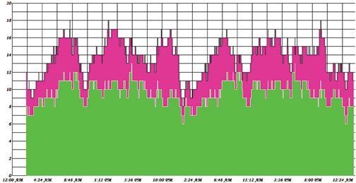


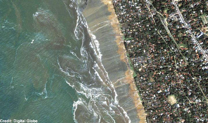

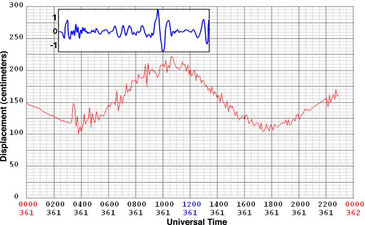
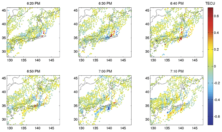
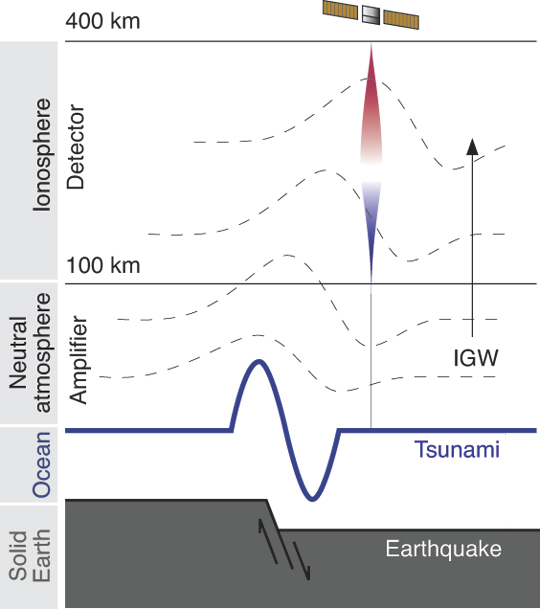
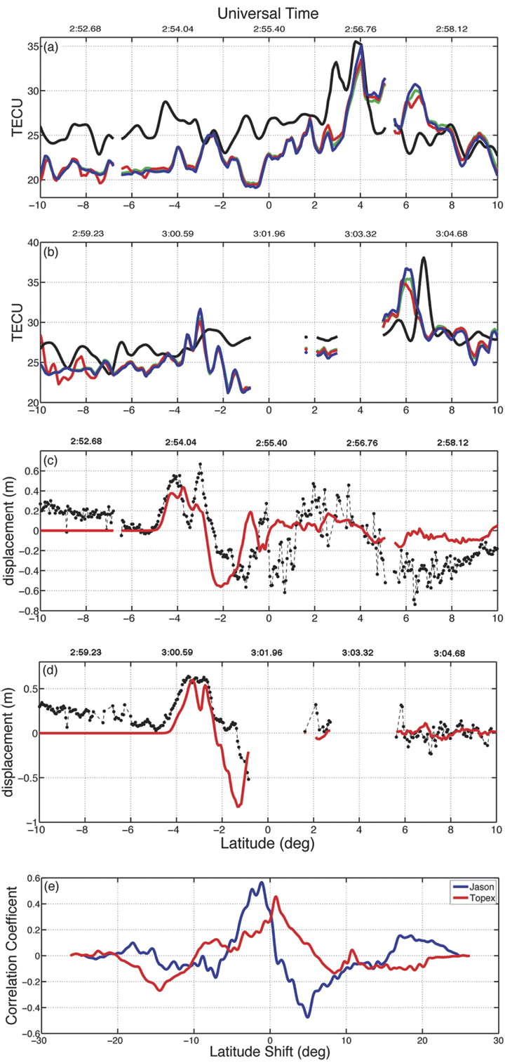
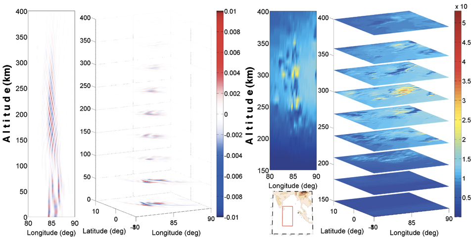
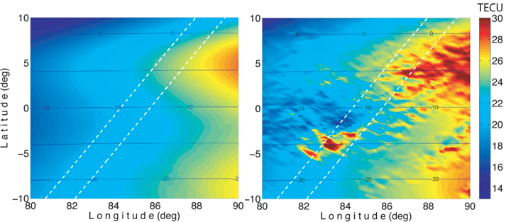
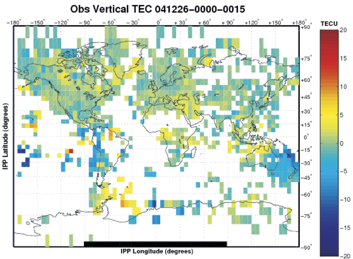


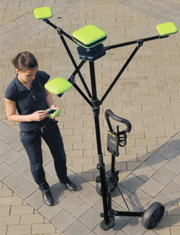