The new European Positioning, Navigation, and Timing (PNT) Industry Council (EPIC) will be a forum for organizations with an interest in all PNT systems including Global Navigation Satellite Systems (GNSS). EPIC shall serve as an information and distribution portal between all stakeholders in the PNT community. Its mandate includes all GNSS constellations and related augmentation systems worldwide, both operational and in development/modernization.
EPIC will undertake to serve the interests of all stakeholders within Europe, and on behalf of Europe on the global stage, recognizing that understanding and cooperation between the world’s stakeholders is key to the successful deployment of new and improved GNSS applications. We also envision that EPIC will become a thriving forum for the exchange of new ideas and best practices, as well as becoming a knowledge center hosting working groups and task forces focusing on specific GNSS issues. EPIC would thus not only serve as a gateway but actually assist stakeholders in developing common solutions to common problems in-house.
Representation
GNSS has applications in many commercial and non-commercial fields: academia, agriculture, airline operators, civil aviation authorities, air navigation service providers, emergency services, energy suppliers, logistics, manufacturing, maritime, communications, petrochemical, rail, surveyors, and more. Therefore, EPIC will work on behalf of all GNSS stakeholders regardless of their application or business model and represents the whole community, integral to the ongoing success of GNSS. In addition it will represent the needs of users and developers of downstream applications.
International
EPIC stands with sister organizations in North America and Asia:
United States GPS Industry Council
Japan GPS Council
Korean GNSS Technology Council
EPIC will maintain close ties to these organizations and will profit from shared practices and knowledge when mutually beneficial. Joint representation with these organizations to government GNSS authorities will be a key coordination activity.
Communication
EPIC will encourage communication and cooperation among its membership to develop new associations and partnerships to create new applications or share ideas and expertise. It will organize regional meetings, workshops, focus groups and social gatherings.
The organization will update members on the latest developments within GNSS and work to ensure that information is made available in a sensible, secure manner and shared as publicly as possible. We intend to keep EPIC a dynamic organization, reflecting the world of GNSS, responsive and adaptable to the needs of its members. Therefore, active involvement from the membership of EPIC will be crucial to its success in both setting the agenda and then realizing it. It is no accident that EPIC is intended as a forum — not just a place for debate but literally a marketplace of ideas where real transformative change can take place.
To get the ball rolling, EPIC will conduct a market survey over the next few months with potential members to clarify their requirements and ensure that EPIC starts with the issues and people that matter.
John Wilde has great experience in the GNSS field, specializing most recently in aviation requirements. He is the founder of EPIC. See also his February 2008 interview on the same subject.
At the Civil GPS Service Interface Committee meeting in Portland, Oregon, on September 20, Sergey Revnivykh, Deputy Director General of Roscosmos’s Central Research Institute of Machine Building, reported on the status and future of GLONASS.
He provided a number of details on the present constellation and how it will be augmented in the future, stressing that GLONASS is doing well and that a full constellation of 24 primary satellites will be in operation within months. The average signal-in-space range error has improved by a factor of five in the past three years and presently stands at about 1.8 meters (one sigma).
Figure 1. The GLONASS satellite generations through GLONASS-K2.
The present constellation consists of 20 healthy satellites with two reserve satellites, GLONASS 714 and 726. Revnivykh stated that GLONASS 726 had a failure of its navigation payload. It is known that the signal generator on the satellite is faulty and it had been set unhealthy since August 31, 2009. Nevertheless, it was placed in reserve status on March 19, 2010. GLONASS 714 is nominally healthy and could be brought back to service if needed. These initial reserve satellites are also being used to train the ground team to operate spare satellites in a full or nearly full constellation.
GLONASS 727, in orbital slot 3, which was taken out of service on September 8, has also had a failure of its navigation payload and may not be returning to service. The three new satellites launched on September 2 are expected to enter service in early October. About 11 more GLONASS-M satellites will be launched by the end of 2012.
Revnivykh announced that there will be two versions of the new GLONASS-K satellites: GLONASS-K1 and GLONASS-K2. GLONASS-K1 satellites will have a 10-year design life and a daily clock stability of 5 x 10-14.
The first GLONASS-K1 satellite will be launched this December from the Plesetsk Cosmodrome about 800 kilometers north of Moscow. This will be the first launch of a GLONASS satellite from other than the Baikonur Cosmodrome. Only one more GLONASS-K1 satellite will be built and launched after that. The K1 satellites will test an open service CDMA signal on the GLONASS L3 frequency in the 1205 MHz band. Although the launch of the first GLONASS-K1 satellite will occur in December, the design process for the CDMA signal structure is not yet finished, according to a subsequent e-mail message from Dr. Revnivykh. When the process is completed, the structure will be made public.
A completely new design, GLONASS-K2, will start launching in 2013. GLONASS-K2 satellites will have a 10-year design life and a daily clock stability of 1 3 10-14. Besides the CDMA signals on L3, CDMA signals will also be transmitted on L1 and L2. The GLONASS-K satellites will transmit the legacy FDMA satellites in addition to the CDMA signals.
A modernized GLONASS-K satellite, GLONASS-KM, for launch after 2015, is now under study. In addition to transmitting legacy FDMA signals on L1 and L2 and CDMA signals on L1, L2, and L3, CDMA signals may also be transmitted on the GPS L5 frequency at 1176.45 MHz. Also being studied is an alternative to the present three-plane, equally spaced satellite constellation. A different constellation design would be possible using CDMA signals. Such a move would require that the legacy FDMA signals be switched off. Revnivykh stated that any such move would require at least 10 years’ advance notice.
The signals that will be transmitted by the future generations of GLONASS satellites as well as those transmitted by the initial GLONASS satellites and the GLONASS-M satellites now on orbit are shown in Figure 2.
Figure 2. Signals transmitted by the different generations of GLONASS satellites. OF 5 open-access FDMA, SF 5 special (military) FDMA, OC 5 open-access CDMA, OCM 5 open-access CDMA modernized.
Revnivykh also spoke on the satellite-based augmentation system under development, System for Differential Correction and Monitoring (SDCM). Correction and integrity data will be transmitted by Luch geostationary communication satellites now under development. Luch 5A, to be launched in 2011 and positioned at 16°W longitude, and Luch 5B, to be launched in 2012 and positioned at 95°E longitude, will transmit signals on an L1 frequency. Luch 4, to be launched in 2013 and positioned at 167°E longitude, will transmit on two frequencies. The three satellites will provide almost global coverage. The satellite payloads are under development.
According to Revnivykh, the SDCM will make use of 12 monitor stations currently in operation in Russia and one in Antarctica at Russia’s Bellingshausen research station. However, the SDCM website indicates only 10 Russian stations currently in the test network. This anomaly might be explained by the fact that some locations have multiple monitor stations. Eight more monitor stations will be added in Russia and five more outside Russia. Revnivykh showed a map revealing the locations of the additional overseas stations as Cuba, Brazil, Vietnam, Australia, and an additional station in Antarctica. It is not intended, at least initially, that these stations would be used in generating the orbit and clock data broadcast by the GLONASS satellites themselves.
Finally, Revnivykh stated that a GLONASS performance document will be released in the 2012–2013 time frame. His full presentation is available on the U.S. Coast Guard Navigation Center website (www.navcen.uscg.gov).
Meanwhile, the three GLONASS-M satellites launched on September 2 have arrived at their designated orbital slots: GLONASS 736, plane 2, slot 9; 737, plane 2, slot 12; 738, plane 2, slot 16.
The operating frequencies are not yet fully known. GLONASS 736, in physical slot 09, is currently undergoing experimental tests. It is included in the broadcast almanac at slot 16 and is transmitting on frequency channel -6. Stations in the International GNSS Service ground network are tracking the satellite. According to the Roscosmos Information-Analytical Centre, when the tests are completed, GLONASS 736 will transmit on channel -2 and be identified as slot 09 in the almanac. It is unclear if GLONASS 736 will replace GLONASS 722 also currently in slot 9, with the latter becoming a spare, or if GLONASS 736 will become the spare as previously inferred.
GLONASS 737 and 738 have not started normal transmissions. Their assigned shared frequency channel is not yet known but -6 would be a likely candidate.
Future GPS Control Segment Advances
The Raytheon Company team developing the next-generation GPS Advanced Control Segment (OCX) successfully completed on schedule an integrated baseline review with the U.S. Air Force.
When completed, GPS OCX will deliver a control segment designed to provide secure, accurate, and reliable navigation and timing information to military, commercial, and civil users. Raytheon is the prime contractor on the $886 million program. The team includes ITT, The Boeing Company, Infinity Systems Engineering, Braxton Technologies, and NASA’s Jet Propulsion Laboratory.
Power Flex Positive
From September 7 to 12, the U.S. Air Force Space Command (AFSPC) activated the long-awaited Flex Power demonstration for GPS, a power increase on L1 and L2. The trial of a new capability designed for military use under special circumstances was deemed a success, essentially going off without a hitch, according to Colonel David Buckman, AFSPC Command Lead for PNT, and Colonel Bernie Gruber, GPS Wing Commander.
Officially, the flex power assessment ensured that the GPS control segment baseline (AEP 5.5) is properly integrated with the space segment with regard to command and control of High-Y Flex Power, a capability that increases the nominal transmit power of the desired signal by shifting power between signals (M-code and P(Y)) within a particular L-band. The net sum gain remains the same. High-Y Flex Power does not change total transmit power, does not affect phase stability between L1 and L2, is ICD-GPS-200E compliant, and does not affect the navigation message.
Only a handful of 10-year-old reference receivers may have been adversely affected, possibly due to an outdated algorithm. Many government, commercial, and civil agencies were involved in the test, and hundreds of GPS receivers were closely monitored. As far as impacts to the overwhelming majority of global users, it was a non-event. The 2nd Space Operations Squadron (2SOPS) was able, over the course of five days, to make power changes to several GPS satellites without causing a phase shift and without the majority of users even knowing what was happening, although various announcements and press releases had appeared to alert them of the fact.
All GPS satellites and signals have now returned to their normal power levels.
Air Force Fends off GAO Zinger
The U.S. Government Accountability Office has issued a follow-up to its alarming and much-criticized report, issued 16 months ago, on the health and prospects of the GPS constellation. Senior officers at the Air Force Space Command and Space and Missile Systems Center have characterized the new report as “overly pessimistic.”
The report’s principal findings — that the Air Force continues to face challenges in launching its satellites as scheduled, which could affect the availability of the baseline GPS constellation, that on-orbit performance of IIF satellites remains uncertain, that a disconnect exists between GPS III and OCX, and that a predicted possible delay in GPS III could affect GPS constellation performance — are discussed and rebutted in detail by GPS World defense editor Don Jewell, with further commentary (paraphrased) by Air Force Space Command, in his October column.
New Galileo ICD Embraced
European Commission (EC) officials held a briefing during ION-GNSS in Portland for industry representatives, to discuss the new Galileo Open Service Signal-in-Space Interface Control Document (OS SIS ICD). Hosts Paul Verhoef and Michel Bosco said they were pleased with what they characterized as positive feedback from U.S., European, and Japanese industry representatives regarding collaboration and consultation over changes made in the ICD. The updated version is available.
The EC grants free access to the technical information on the future Galileo open service signal: the specifications manufacturers and developers need to process data received from satellites. Anyone who wishes to use the intellectual property rights contained in the document simply needs to send an e-mail to [email protected] mentioning their request for a license agreement, which is without any exclusivity or geographic limitation.
FAA Green-Lights ADS-B
The U.S. Federal Aviation Administration (FAA) gave the go-ahead signal for full-scale, nationwide deployment of the satellite-based surveillance system called Automatic Dependent Surveillance – Broadcast (ADS-B) following its successful roll-out at four key sites. Air traffic controllers are now able to use the new technology to separate aircraft in areas with ADS-B coverage. Controller screens in those areas will show aircraft tracked by radar as well as aircraft equipped with ADS-B avionics, which broadcast their positions.
The new system tracks aircraft with greater accuracy, integrity, and reliability than the current radar-based system, the FAA said. ADS-B targets on controller screens update more frequently than radar and display information including aircraft type, call sign, heading, altitude, and speed.
Nationwide ADS-B coverage is scheduled to be complete in 2013. According to the FAA, every part of the country now covered by radar will have ADS-B coverage. More than 300 of the approximate 800 ADS-B ground stations that will comprise the entire network have been installed.
By 2020, aircraft flying in controlled airspace in the U.S. must be equipped with ADS-B avionics that broadcast their position.
The use of a precise wide-area positioning technique for airborne trajectory solutions for LiDAR surveys provides both relative and absolute accuracies similar to those derived from using a local GNSS reference station.
Airborne light detection and ranging (LiDAR) surveys are among the most advanced means of producing high-resolution, accurate surface elevation models used for many applications in surveying and civil engineering. Precise geolocation and orientation (or georeferencing) of the LiDAR instrument with a combination of on-board GNSS and inertial sensors at the times when the measurements are made provides the key to high-quality elevation products.
The usual practice deploys reference GPS/GNSS land receivers in the area where the aircraft will be flying, to obtain a precise trajectory by short-baseline differential GNSS techniques. This could mean installing and operating receivers at many sites during a flight mission if the area surveyed is a large one.
We have tried a different approach: using as reference receivers those of a sparse network of Continuously Operating Reference Stations (CORS) in New South Wales known as CORSnet-NSW, and a wide-area differential GPS technique for obtaining the aircraft trajectory with sub-decimeter accuracy even with baseline lengths of several hundred kilometers. This may be comparable in precision and accuracy to the short-baseline method, but without the cost and logistical complications. This opens up a new level of operational capability, allowing flexibility for weather conditions and priority response applications.
The tests described here were organized and conducted by the NSW government’s Land and Property Management Authority, in collaboration with the University of New South Wales, in June 2009. CORSnet-NSW consists, at this writing, of 46 stations and by 2012 will provide statewide GNSS positioning infrastructure across NSW with a planned 70 stations in operation.
Precise Wide-Area Positioning
We used a technique for long-baseline differential, off-line positioning, able to deliver centimeter precision for fixed receivers and sub-decimeter precision for moving receivers. This choice was dictated by three considerations:
The intended application was the geolocation of the data of an airborne scanning LiDAR sensor to be used in the generation of high-accuracy digital elevation models (DEM).
Off-line processing, where all the GNSS data collected during the flight are available for processing and (as in this case) there is no need for immediate results, is intrinsically more reliable than real-time processing, where the data are available only up to the present epoch, and accurate results must be obtained right away, with no chance for a second try.
Differential processing makes it possible to resolve the carrier-phase ambiguities using well-understood methods.
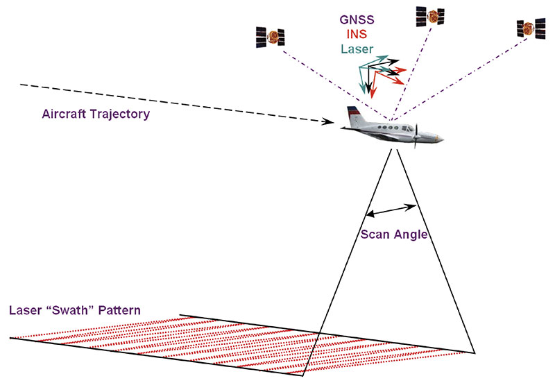
Technique. It is common practice in airborne LiDAR surveys to use GNSS both to position the instrument precisely, and to assist an inertial navigation system (INS) to obtain the orientation of the aircraft in space, as both position and orientation are needed to interpret the data properly. FIGURE 1 illustrates the relationship between the sensors used for airborne LiDAR surveys. The aircraft uses a GNSS antenna combined with an INS to georeference its trajectory. The bore-sight calibration process aligns the individual sensor orientations and standardizes the range measurements. However, if the survey is to achieve the now-expected high level of vertical accuracy (615 centimeters, 1 sigma), then the position of the GNSS/INS-derived aircraft trajectory for each laser swath must be determined with a relative precision in the order of just a few centimeters. This is achieved via differential GNSS post-processing of the kinematic airborne data together with static observations collected on precisely surveyed ground reference stations. The GNSS positions are then blended with high-frequency measurements taken by the onboard INS to produce the final trajectory and reference orientations.
Figure 1. Airborne LiDAR reference frame.
To such ends, the aircraft trajectory is usually determined by short-baseline differential GNSS, with ground receivers deployed near the intended flight path of the aircraft. In this way it is possible to use GNSS data analysis techniques that are both precise and quite straightforward to implement in software. The simplicity of these techniques is possible because, in short-baseline differential solutions, the data of the aircraft receiver and any nearby network receivers have much the same systematic errors (due to such things as satellite ephemerides errors, transmission delays, and so on) that cancel out — or nearly so — when their observations are differenced between them. This also makes it possible to resolve quickly and reliably the cycle ambiguities in the observed carrier phase, the most precise type of GNSS data, overcoming one of the main obstacles to obtaining good results. Furthermore, it is possible to get such results with single-frequency receivers, as ionospheric delay is one of the systematic effects that can be largely canceled out.
In wide-area solutions, those cancellations are not complete enough to ignore the systematic data errors, and they have to be included in the form of additional unknown parameters in the observation equations. Also, it is necessary to account for the ionospheric delays using dual-frequency data, which means using more expensive GNSS receivers and antennas.
Resolving the carrier-phase ambiguities is no longer straightforward or assured. The standard way of dealing with the ambiguities is to include them as unknowns in the observation equations and adjust them along with the other unknowns: this is often referred to as “floating the ambiguities.” Fixing (or resolving) those ambiguities to their most likely integer values in a matter of seconds to a minute is possible on occasion, when the aircraft is within less than 20 kilometers from a ground receiver, or very precise corrections for the ionospheric delay are available; otherwise slower techniques, that require tens of minutes, may be used. It is also necessary to correct as well as possible such things as the neutral atmospheric delay of the GNSS radio signals, the movement of the “fixed” stations due to plate tectonics, the solid earth tide using mathematical models, and, in the case of the tropospheric delay, estimating the error in the corrections made using a standard formula as an additional unknown per receiver.
Over the years all these difficulties have been gradually dealt with more effectively, more efficiently, more reliably and, from the user’s point of view, less painfully. Originally developed for the repeated determination of station positions to measure the slow tectonic deformations of the Earth’s crust, and to calculate precisely the orbit of Earth-observing satellites, these days, after nearly 30 years of steady progress, GNSS wide-area techniques and the corresponding software find many applications in science, engineering, and navigation, and are becoming widely used in remote sensing.
Software. We used the Interferometric Translocation (IT) wide-area positioning software developed by one of us for the long-baseline aircraft trajectory solutions and also to re-position in the IGS05 international reference frame some CORSnet-NSW stations, so their data could be used consistently in the differential wide-area solutions. These stations were originally given in the Geocentric Datum of Australia (GDA94). For both purposes we used the precise final GPS orbits computed and distributed by the IGS.
To validate the aircraft trajectories calculated with the wide-area method, we relied mainly on the quality of the LiDAR DEM results obtained with those trajectories. We also used commercial software to generate short-baseline differential solutions with receivers deployed near the intended aircraft flight-path, as is common practice in this type of survey, and compared them with the wide-area solutions (they turned out to be quite similar to short-baseline solutions obtained with the wide-area software).
Airborne Tests
This study has used data from two airborne LiDAR surveys conducted by the NSW Land and Property Management Authority (LPMA) in June 2009. The first took place near the township of Glen Innes, and the second was a bore-sight calibration flight near the city of Bathurst. For both LiDAR surveys, the following data were acquired:
Aircraft trajectory, raw dual-frequency GPS (1 Hz) and IMU data (200 Hz).
LiDAR (raw return data for each laser pulse).
GPS reference station data from local receivers and multiple CORSnet-NSW sites.
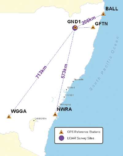
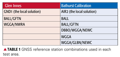
Glen Innes Test. This operational LiDAR survey established GND1 as the local reference station within the survey area. CORSnet-NSW data were collected for the test from GNSS receivers in Ballina (BALL), Grafton (GFTN), Nowra (NWRA), and Wagga Wagga (WGGA). FIGURE 2 shows the distribution of the reference stations and the flight runs.
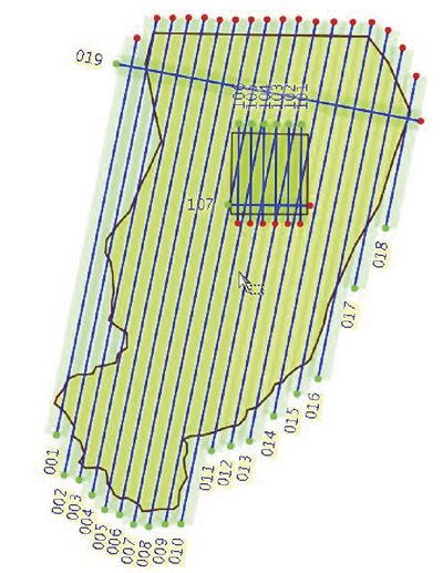
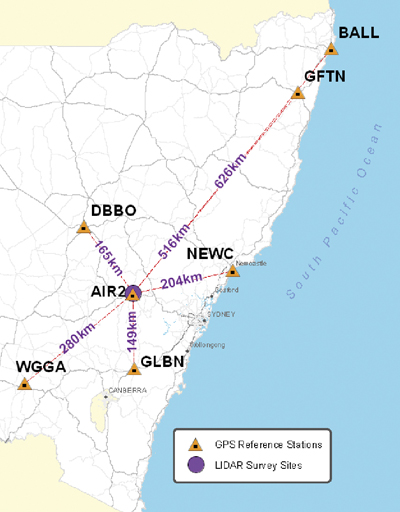
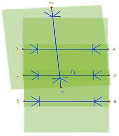
Figure 2. Glen Innes survey of June 9, 2009, showing the distribution of reference stations with baseline lengths and the survey area with (numbered) flight runs.Bathurst Test. Bathurst Airport is LPMA’s LiDAR calibration site and has various arrays of accurate ground checkpoints. AIR2, near the runway of the Bathurst airport, is the locally established GNSS reference station. CORSnet-NSW data were collected for the test from receivers in Ballina (BALL), Dubbo (DBBO), Grafton (GFTN), Newcastle (NEWC), Nowra (NWRA), and Wagga Wagga (WGGA). FIGURE 3 shows reference-station distribution and a schematic of the flight runs.
Figure 3. Bathurst test of June 16, 2009, showing the distribution of reference stations with baseline lengths and the survey area with (numbered) flight runs.
Effect on LiDAR Data
Rather than simply comparing aircraft trajectories, this study aimed to determine what effect the use of wide-area GNSS positioning has on the actual LiDAR point data and associated elevation surfaces. In terms of the horizontal accuracy required for LiDAR surveys, initial tests showed that the differences between the horizontal positions of various trajectories was negligible; therefore, only the vertical component was considered in this analysis.
To quantify differences between LiDAR data generated from trajectories using various combinations of distant GNSS reference sites, we applied four types of analysis:
Comparison of trajectories — directly compare the locally computed trajectory (assumed to be truth) with each wide-area derived trajectory.
Relative LiDAR point comparison — compare the positions for a sample of LiDAR ground points derived from the locally computed trajectory with those derived from each wide-area derived trajectory.
DEM comparison — difference the raster surfaces derived from the locally computed trajectory and a wide-area derived trajectory to find the effect over a LiDAR run.
Absolute LiDAR ground control comparison — compare the LiDAR derived surface from various trajectories to the surveyed ground control (Bathurst Calibration test site only). This also involves vertically shifting the resulting surface so that its offset relative to the one used as control is zero, thus removing the effect of using different reference frames for the GNSS trajectories and the control surface.
Trajectory Comparison
The comparison between the locally determined and each wide-area derived trajectory was made along the entire trajectory for each flight. The importance of this step lies in the assumption that all LiDAR data are directly positioned from the trajectory and so any systematic effect in the trajectory should be reflected on the ground. For each test site the locally derived solution is assumed to be “truth” with the vertical difference computed against wide-area solutions for each combination of reference stations used (TABLE 1).
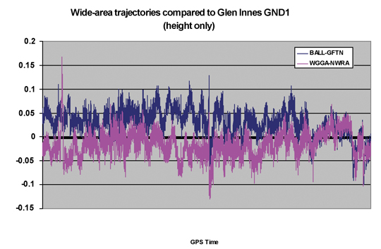
Glen Innes Test. FIGURE 4 shows the vertical comparison of two wide-area derived trajectories (using BALL and GFTN, and WGGA and NWRA, respectively) against the locally derived trajectory (using GND1). It can be seen that once the aircraft attained its stable operating altitude, the wide-area derived trajectories are generally within 5 centimeters of the locally derived solution.
Figure 4. Trajectory elevation differences for entire Glen Innes flight.
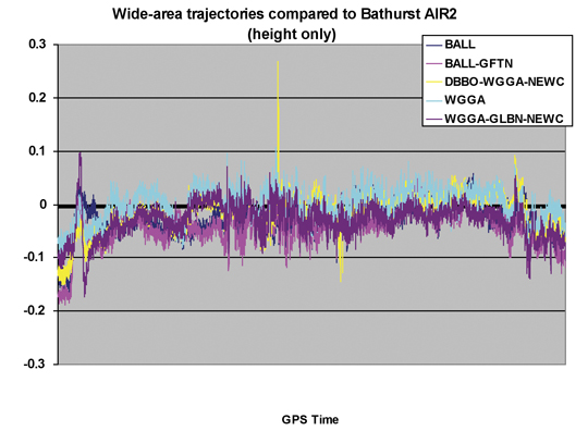
Bathurst Test. The Bathurst test differs from the Glen Innes test in that both the duration of the flight and the length of each run are significantly shorter. FIGURE 5 shows the vertical component of five wide-area derived trajectories, using several combinations of CORSnet-NSW reference stations, compared against the locally derived trajectory (using AIR2). The results once again show a remarkably consistent comparison with the locally derived solution. Data spikes showing up in the DBBO/WGGA/NEWC (yellow) solution were attributed to small data glitches at the DBBO CORSnet-NSW site. Unfortunately, LiDAR data were not collected at those instances; therefore, the effect on ground data could not be fully assessed.
Figure 5. Trajectory elevation differences for entire Bathurst calibration flight.
Relative Comparison
Regardless of the trajectory and orientation used to georeference LiDAR data, the same number of points will be created. It is therefore possible to create a LiDAR dataset using the same raw LiDAR data but different GNSS trajectories, and compare the results to determine the relative positioning differences on the ground.
Given the large number (many millions) of points in a LiDAR dataset, we used a representative sample of evenly spaced 10 2 10 meter areas each containing 50–100 points (on level ground) for statistical analysis. We calculated displacement vectors between points computed from the locally derived trajectory and those using wide-area trajectories. Results from flight run 002 at Glen Innes (see Figure 2) and run 7 at the Bathurst Calibration test site (see Figure 3) are presented here.
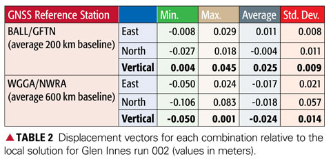
Glen Innes Test Run 002. The displacement vectors from 46 sample areas (4,620 points) are summarized in TABLE 2, being points computed using the two wide-area solutions compared with the locally derived solution using reference station GND1. Note the high accuracy achieved in the all important vertical component.
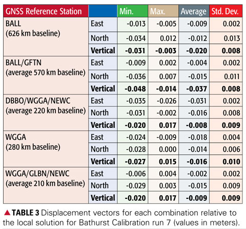
Bathurst Test Run 7. The displacement vectors from 25 sample areas (1,700 points) are summarized in TABLE 3, being points computed using the five wide-area solutions compared with the locally derived solution using reference station AIR2. Once again the results clearly show that the height values agree to within a few centimeters, even over baselines of more than 600 kilometers in length.
DEM Comparison
To investigate how the LiDAR surfaces derived from each trajectory compare across the entire data swath, we created raster surfaces from the LiDAR point data. Each surface was then subtracted from the local solution to create a difference surface. Visual inspection and interpretation was then used to discern any patterns or effects.
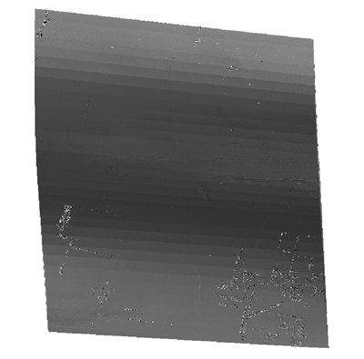
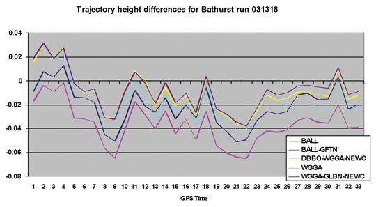
The result shown in FIGURE 6 (Bathurst Calibration flight run 7) was typical of the cyclical effect evident for all solutions. The magnitude of the difference was in the order of 2–3 centimeters and is in the direction of flight (north to south). If this cyclical variation is compared with the trajectory comparison for just the 33-second duration of flight run 7, a clear (expected) correlation with the variation in height is evident (FIGURE 7).
Figure 6. Subtraction surface for Bathurst Calibration run 7 (AIR2 vs. BALL).Figure 7. Trajectory comparison for Bathurst Calibration run 7 (031318).
No DEM comparison results are presented for the Glen Innes data because of significant variation in terrain and vegetation, making interpolation difficult and unreliable.
Absolute LiDAR Comparison
Ground control points serve two purposes in a LiDAR survey:
The calculation of statistics to describe vertical accuracy, that is, quantifying the match of the surface to the local height datum.
The calculation of a surface adjustment to enable transformation of the LiDAR points to fit the local height datum.
Additionally, ground control points with accurate heights are used to calibrate the sensor before use in active LiDAR surveys to account for internal electrical delays in the ranging and measurement system. LPMA maintains a calibration site at Bathurst Airport for this purpose, and regularly surveys the area to ensure the sensor is operating at maximum accuracy. It should be noted that the sensor was calibrated using Bathurst Airport ground control data prior to this study.
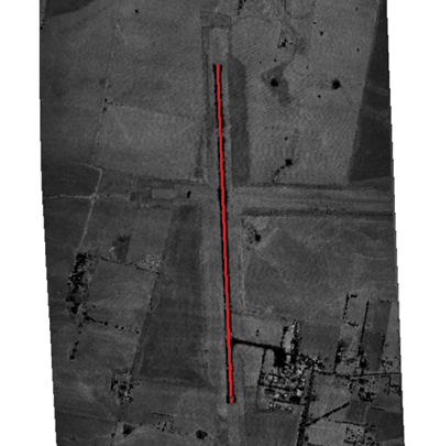
Surveyed Ground Control. The airport runway centerline vertical profile for the Bathurst Calibration site (FIGURE 8) was re-computed in terms of the same IGS05 reference frame determined for the LiDAR trajectories, thereby allowing an independent comparison with ground truth.
Figure 8. Runway vertical profile at the Bathurst Airport calibration site.
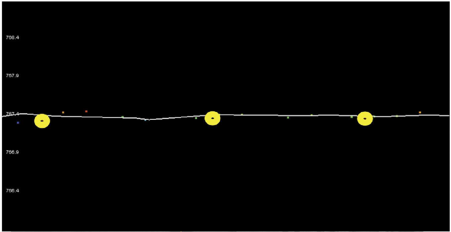
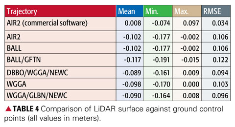
Point Comparison. Data from Bathurst run 7 were used to compare LiDAR results with the established ground control using a basic triangulated irregular network (TIN) surface comparison (FIGURE 9 and TABLE 4). In Figure 9, the TIN surface is indicated by the white line, while the ground control points are shown with yellow buffers.
Figure 9. Comparison of LiDAR surface and ground control points.
The first trajectory in Table 4 is the original calibration comparison using commercial software and orthometric height data. All wide-area solutions display a similar vertical offset, because of the use of different reference frames for the GrafNav and wide-area solutions (IGS05 vs. GDA94), and differences in the implementation in software of, for example, antenna corrections and atmospheric modeling. At first glance, the significant differences to the GrafNav trajectory caused the wide-area result to not satisfy the accuracy specifications for LiDAR. However, had the wide-area solutions been used for the sensor calibration, the figures would have been much closer to the ground truth.
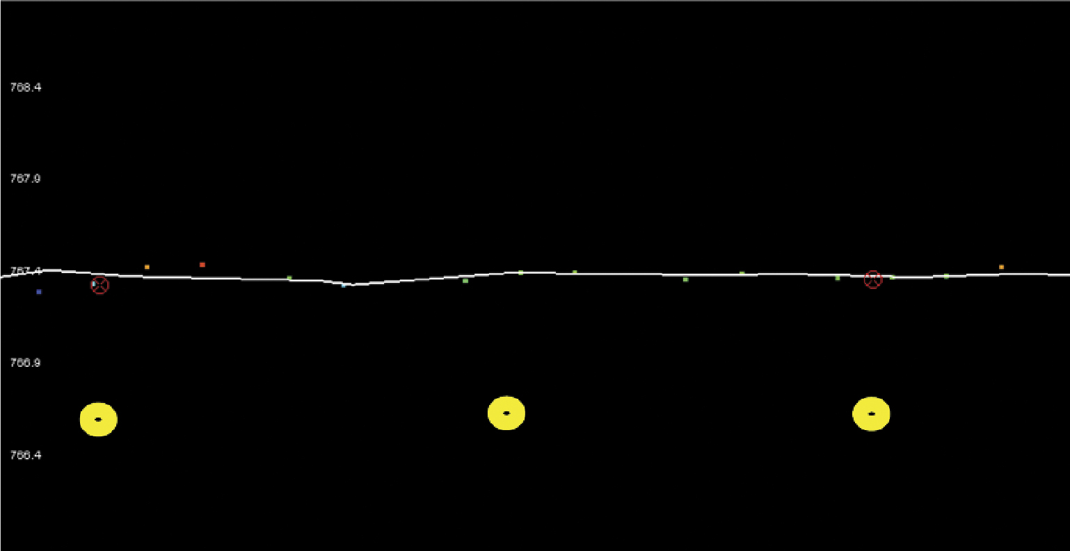
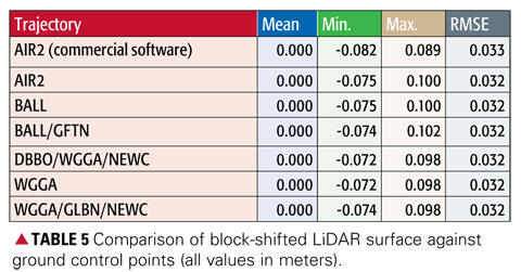
Block-Shifted Data Comparison. In an operational environment, because of systematic errors in the resulting DEM relative to the local height datum, this mean vertical offset is a common occurrence with comparisons against ground control similar to those shown in FIGURE 10. Again, the TIN surface is indicated by the white line, and the ground control points are shown with yellow buffers.
Figure 10. Usual operational comparison of LiDAR surface and ground control points.
In standard LiDAR operations, the mean vertical offset between the initial results and the ground control, at the control points, produces a zero-mean offset. Following this procedure in this case results in the variation in the comparison of LiDAR data with ground truth now being well within the required limits of 615 centimeters (TABLE 5). The values show that after a block shift, trajectory solutions are virtually identical with a root mean square error of 32 millimeters. Thus, local GNSS reference stations can be replaced by distant CORS sites without loss of accuracy.
Conclusions
A precise wide-area positioning technique for airborne trajectory solutions provides both relative and absolute accuracies similar to those derived from usinga local GNSS reference station. Irrespective of which reference sites are used and once calibration and antenna modeling issues are addressed, the absolute comparison with ground control is well within the required accuracies. With the configuration of a GNSS network such as CORSnet-NSW (when complete, at least one site will always be within 150 kilometers of any point within New South Wales), an airborne LiDAR survey in the network’s service area can provide data for computation of an accurate sensor trajectory. This potentially negates the need to place and maintain ground reference stations close to the survey area — an exercise which not only requires significant resources but also reduces the operational flexibility of the aircraft.
The challenge for this technique in an operational environment is to define and maintain a precise reference frame for all CORSnet-NSW sites and observations, including the use of a stable ellipsoidal height datum with compatible geoid modeling in order to provide local orthometric elevation data. The knowledge base required for computation of wide-area GNSS solutions is significant and requires understanding of geodesy, GNSS positioning, absolute antenna modeling, application of precise ephemerides, and derivation of the other parameters inherent to successful ambiguity resolution over long distances.
Regardless of processing method, a LiDAR survey will always require independent ground surveys for collection of vertical checkpoints, which provide quality control to ensure the accuracy meets specifications, and the means to define any transformations necessary to fit LiDAR data with local height datum.
Manufacturer
NovAtel’s WayPoint GrafNav software was used for comparison purposes.
The ”IT” Software
Runs under Windows, Unix, Linux, and FreeBSD.
Source code compatible with most Fortran compilers.
Follows the IERS 2003 conventions.
Available mainly for collaborative research purposes, with a Free Software Foundation General Public Lice
nse.
Stop-and-go for rapid mobile surveys with pre-surveyed waypoints.
Differential, precise point positioning, mixed mode (precise differential + point positioning).
Data corrected for: Earth tide, neutral atmosphere radio signal delays, carrier phase windup, and so on.
Estimated parameters:
Receiver position in the IGS05 reference frame, with the WGS84 reference ellipsoid, earth spin-rate, light speed, GM constant.
Biases in ionosphere-free carrier-phase linear combination (“floated” ambiguities).
Neutral zenith delay correction error.
Broadcast orbit errors (allows precise differential near-real time solutions).
Integer ambiguity resolution available in differential mode, with short baselines up to 20 kilometers (in minutes), and baselines of unlimited length (in tens of minutes — or just minutes, with a precise ionosphere correction).
Oscar L. Colombo received a degree in electrical engineering from the National University of la Plata, Argentina, and a Ph.D. in electrical engineering from the University of New South Wales, Australia. He is an independent consultant.
Shane Brunker is an airborne LiDAR and imaging specialist working in a consulting capacity for specialized LiDAR survey company Network Mapping (United Kingdom).
Glenn Jones is a senior surveyor at the NSW Land and Property Management Authority in Bathurst, Australia.
Volker Janssen is a GNSS surveyor (CORS Network) in the Survey Infrastructure and Geodesy branch at the NSW Land and Property Management Authority in Bathurst, Australia. He holds a Ph.D. from the University of New South Wales.
Chris Rizos is head of the School of Surveying and Spatial Information Systems of the University of New South Wales, has a surveyor’s degree and a Ph.D. from the same university, and is an specialist in geodesy and GNSS positioning.
By Chaminda Basnayake, Tom Williams, Paul Alves, and Gérard Lachapelle
Communication-enabled vehicle safety has the potential to change transportation’s future, particularly vehicle-to-vehicle (V2V) and vehicle-to-infrastructure (V2I), collectively represented as V2X. An automakers’ consortium conducted extensive field trials to determine GNSS service availability and accuracy for the V2X challenge.
V2X can include applications based on communications between any two or more entities on the road. Of all the potential V2X applications, V2V applications probably lead the way in terms of maturity of prototype development and test efforts. General Motors (GM) demonstrated the first working prototype V2V system in 2005. Information on further industry collaborative efforts in V2V system developments can be found at the U.S. Department of Transportation’s (DOT’s) IntelliDrive website. While a multitude of applications could be developed based on V2I capability, most of the related system prototype development efforts have taken place under the DOT’s Cooperative Intersection Collision Avoidance (CICAS) program.
Driving environments encountered in testing. Clockwise from top left: deep urban, urban thruway, local roads, mountains.
Accuracy Requirements
In terms of positioning accuracy requirements, Vehicle Safety Communications-Applications (VSC-A) prototype system capabilities as well as all V2X applications can be classified as:
Which Road. In this case, accuracy is only required to the extent of identifying the road traveled. For instance, if a vehicle is in a service road parallel to a freeway, knowing that it is on the service road and not on the freeway is sufficient. The need of a typical vehicle navigation device is another good example of this requirement category. The typical accuracy requirement for this case is better than 5 meters. However, this could be a relative accuracy requirement for certain applications. For instance, in a V2V scenario, one vehicle may only need to know if the other is on the same road or not, while in the absolute sense both vehicles could be in error by more than 5 meters. For V2I applications, however, this becomes an absolute accuracy requirement, as the infrastructure is always mapped and identified with respect to a global coordinate frame.
Which Lane. This accuracy level enables applications to identify other entities with lane level resolution. The typical requirement is 1.5 meters or better, which approximately corresponds to half of a lane width. A blind-spot advisor is a good example that requires this accuracy.
Where-in-Lane. This accuracy level enables the relative positioning of entities to better than 1 meter. Further refinements of blind-spot advisor-like applications are examples.
Availability Requirements
GNSS as a line-of-sight technology has obvious limitations in certain environments, and these limitations are well understood by the GNSS community. The focus of this study was to understand the limitations associated with a GNSS-only V2X solution such that requirements for augmentation technologies can be defined. Therefore, no availability requirements were set for the system; estimating availability of a GNSS-only solution was the goal.
Why So Complicated? At first glance, what needs to be done is straightforward; all V2X-capable entities need to be aware of each other’s positions. Hence, if all entities transmit their own location with respect to the same coordinate system, the problem is solved. Unfortunately, it’s not that simple.
Designing the system so that hundreds of entities, potentially using all sorts of GNSS software and hardware, can work together presents a significant challenge. This includes keeping backward compatibility way out into the future.
Even within the same receiver make and type, inclusion of a particular satellite in the solution of one vehicle can significantly affect the solution difference between vehicles. Inclusion of SBAS also contributes as a differentiator. In a V2X scenario, out of two adjacent vehicles, one vehicle may use SBAS while the other may not, due to hardware configuration or visibility. If none of the above situations occurred and everything else were ideal, transmitting just the current horizontal position of a V2X entity over-the-air (OTA) would be sufficient to do everything needed.
V2X thus requires a positioning system architecture that minimizes the impact of these complications and many other potential compatibility issues. Major system design considerations include:
Performance Requirements. The system must provide relative positioning accuracy that fits Which Road, Which Lane, or Where-in-Lane category and should identify the solution quality. For instance, a vehicle on a freeway with relatively open sky view may function in the Which Lane mode and may transition to Which Road mode as it enters an urban area with sky visibility limitations.
Deployment Constraints. The system must be affordable for automotive applications. This may also include considerations such as antenna placement, processing resource requirements, and power requirements.
Bandwidth Constraints. The volume of data transmission constitutes a major consideration for OTA communications. While some methods manage communication range and frequency as a way of optimally using the communication channels, keeping the OTA data volume to a minimum by design was a goal.
Study Goals
This study investigated the performance of two relative positioning methods: DPOS, a method of using the difference in position reported by two entities to calculate the 3D separation between the points; and real-time kinematic (RTK). While there are many other possible relative positioning methods, these two were selected as they collectively represent the most desirable availability and accuracy performance. In DPOS, vehicle coordinates are transmitted between vehicles in order for position differences between vehicles to be derived at each vehicle. In RTK, raw code and carrier-phase data is transmitted between vehicles, and the inter-vehicle position differences are calculated using RTK software in either fixed or float carrier-phase ambiguity mode at each vehicle. The RTK method is more intensive both from a data transmission and computational aspect, but retains only common satellites in the solution, eliminating the problem described earlier. Its use of carrier-phase measurements also makes it more accurate.
The study included two GPS receiver types. The first, a single-frequency L1 automotive-grade receiver, is identified as Type B receiver in this study. The second, identified as Type A, was of a higher quality with proprietary multipath mitigation technologies. Both receivers were capable of using WAAS support. Receiver B also allowed the user to reject selected satellites from its solution. These two devices were selected as they were capable of supporting both processing methods, and represent on the one hand an existing automotive-grade receiver, and on the other hand one that is expected to be a good representation of a product with technologies available for automotive deployment a few years from now.
Specific study goals were:
Accuracy performance of DPOS and RTK methods when all vehicles use same GPS receiver type.
Same when a receiver type or a receiver configuration mix is used.
Dependency of the accuracy performance on the driving environment.
Solution availability with same receiver and mix receiver combinations.
Implications of non-continuous V2I coverage.
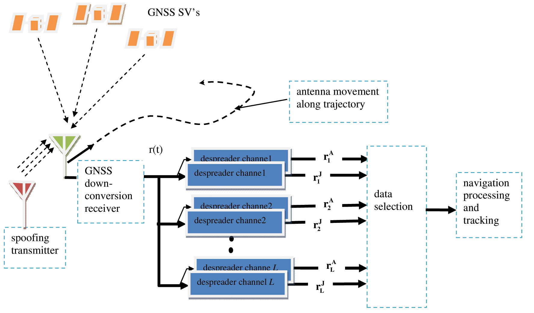
Prototype System
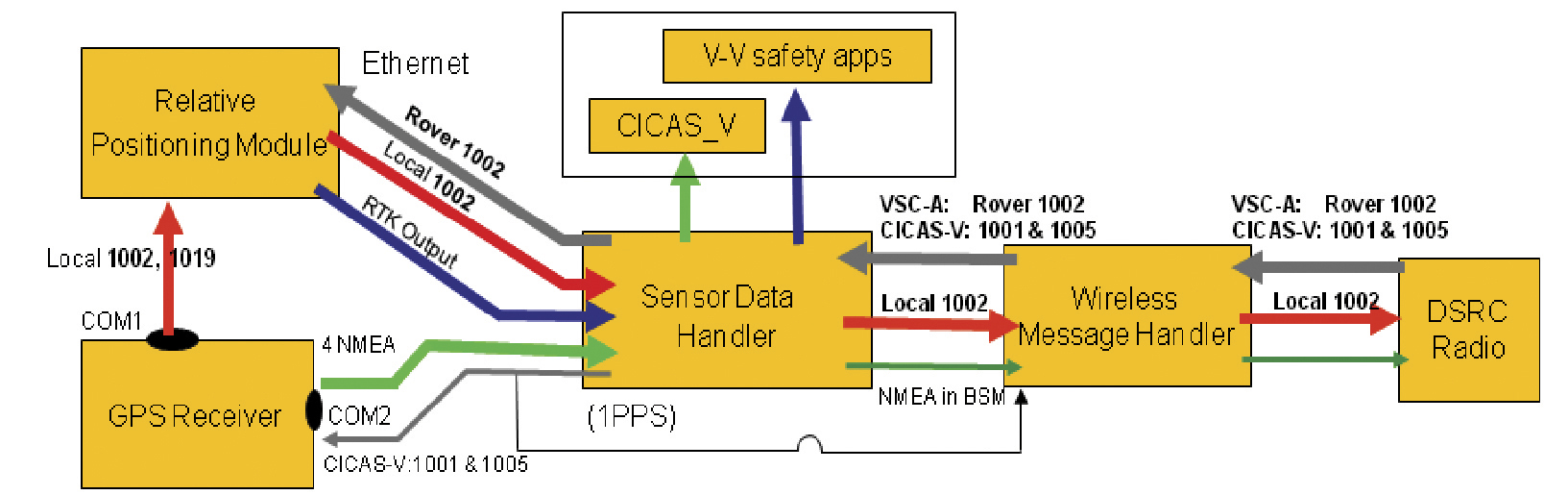
The system prototype (Figure 1) used for the study was a replica of the prototype relative positioning system implemented in the VSC-A project. It consists of a dedicated short-range communicatin (DSRC) interface with a DSRC radio, a GPS receiver/relative positioning module, and a sensor data handler.
In operation, a vehicle generates its own location information and GPS raw data in RTCM format and shares this data with other vehicles. OTA messaging was done using the SAE J2735 messages set with GPS raw data in RTCM format attached as optional data. As shown in Figure 1, RTCM v3 1002 messages were used to exchange VSC-A data. The system was also capable of using RTCM v3 messages 1001 & 1005 for V2I operation. The DPOS relative positioning logic was implemented in the sensor data handler, while the RTK implementation was done in a separate relative positioning module. This module takes in local and remote 1002 messages and outputs RTK data to the sensor data handler. Applications could access both RTK and DPOS relative positioning information from the sensor data handler.
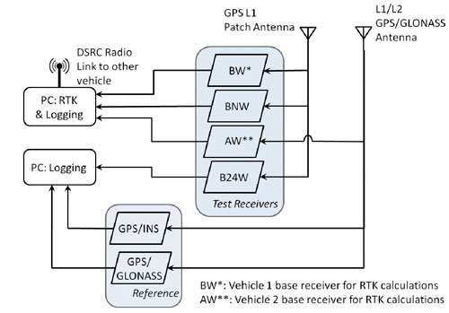
Vehicle Setup. Two vehicles were used for the V2X data collection. Four different GPS L1-only test receiver types were installed on each vehicle:
AW: high-quality receiver using WAAS corrections.
BW: high-sensitivity automotive-grade receiver with WAAS ranging and corrections enabled.
BNW: high-sensitivity automotive-grade receiver with WAAS ranging and corrections disabled.
B24W: high-sensitivity automotive-grade receiver using a maximum of the four primary satellites in each of the six planes (minimum guaranteed constellation) and with WAAS ranging and corrections enabled.
As shown in Figure 2, the AW and B type receivers were connected to different GNSS antennas. These antennas were mounted on roof-racks attached to the vehicles (see Photo). The patch antenna for the Type B receivers was mounted on an aluminum-topped wooden pedestal to bring it to approximately the same height as that used by the AW receivers, to provide a ground plane and to prevent shading from other equipment on the roof-racks. The spacing between the antennas was accounted for in all analysis.
Figure 2. High-level V2V hardware setup on each of the two test vehicles.
Figure 2 also shows that only three of the four test receivers, AW, BW, and BNW, were connected to the computer that ran the RTK software. This computer calculated the inter-vehicle vector (IVV) using information exchanged over the DSRC radio link in real time. The vehicles each had a designated base relative to which the IVV was calculated; for Vehicle 1 it was BW and for Vehicle 2 it was AW. Thus the computer on each vehicle calculated three instances of the IVV, for example, the computer on Vehicle 1 calculated BW1–BW2, BW1–BNW2, and BW1–AW2 (where Ri denotes the receiver of type R on vehicle i).
Transmission and reception of data between the two vehicles required for the IVV RTK calculations were achieved using wave radio modules with two magnetically mounted 802.11p antennas on each vehicle for redundancy. During testing, Vehicle 1 generally followed Vehicle 2. To minimize potential interference of roof-mounted instruments on between-vehicle communications, the antennas on Vehicle 1 were located close to the front of the roof, while those on Vehicle 2 were located close to the rear of the roof. In each case, 15 centimeters of roof space were left to provide ground planes for the antennas.
We used the single-point navigation solutions logged from each test receiver to calculate the IVV for each receiver combination using the DPOS method in post-processing. No real-time data transfer between the vehicles was used for this method.
Reference values of the IVV were calculated in post-processing using both geodetic grade GPS/GLONASS L1/L2 receivers and GPS/INS integrated systems in differential mode. Both were connected to the antenna used by the AW receiver. Differential GPS calculations were enabled by using stationary receivers with antennas at precisely known WGS84 locations on top of a building at the University of Calgary.
Two study vehicles with antennas attached to the roof-racks.
Test Scenarios
V2V data was collected in and around the city of Calgary in August 2009. In the majority of the tests, Vehicle 1 followed Vehicle 2 with a separation of less than 300 meters, the stated effective range of the DSRC link. For most tests the inter-vehicle separation was between 30 and 150 meters. Some driving environments forced modifications of the default behavior; for example, on highways, vehicles moved in between the two test vehicles, necessitating lane changes. Approximately 52 hours of data was collected over 12 days. After rejecting data due to various faults such as reference-system malfunction, more than 45 hours of data remained.
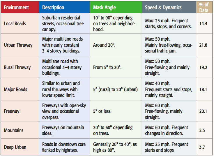
Data was collected in the seven test environments listed in Table 1. These environments were selected in accordance with Federal Highway Administration descriptions. Each environment provided different challenges for GNSS-based positioning. Obviously the deep urban environment was challenging because the reduced number of visible satellites and the large amount of multipath meant that navigation solutions were both rare and of poor quality. As another example, the mountain environment was interesting because often almost half the sky was occluded by trees on the mountain side, leading to an asymmetrical visible GPS satellite constellation with the associated solution degradation. The photos at the beginning of this article show selected driving environments encountered during testing.
Table 1. Description of driving environments used in V2V tests.
V2V Solution Accuracy. Positioning accuracy of the individual receiver was first investigated to estimate the V2V relative positioning accuracy when using the DPOS method. This was done for the entire dataset.
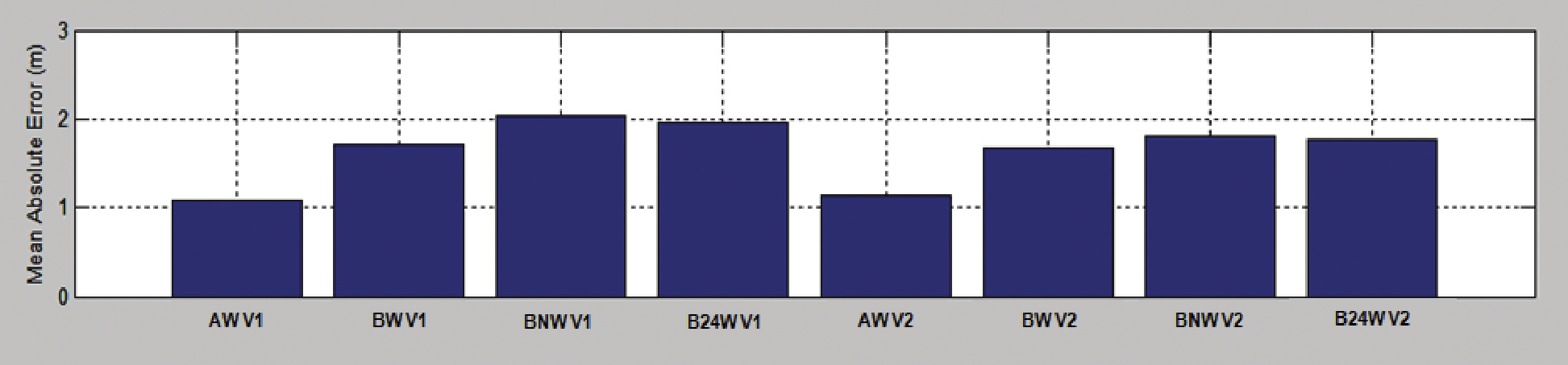
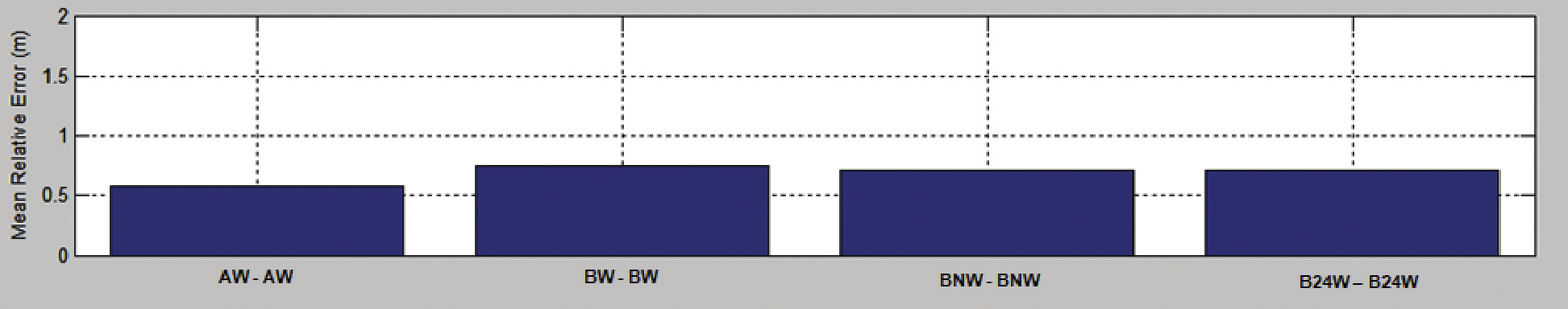
Figure 3A shows a representative freeway dataset to illustrate overall trends: the absolute 2D mean position errors observed from all eight GPS receivers used in both vehicles. The first set of four receivers shown were the AW, BW, BNW, B24W receivers in the first vehicle (V1), and the second set of receivers were the same type in the second vehicle (V2). As a general trend, Type A receivers provided better absolute accuracy meeting the Which Lane accuracy, whereas the Type B receivers provided Which Road accuracy. Also, the use of WAAS with receiver Type B has yielded some absolute accuracy improvement. Limiting the constellation to 24 (B24W) did not significantly degrade accuracy in this case.
As a second step, V2V relative accuracy when the same receiver type was used was estimated, and the mean errors are shown in Figure 3B. Based on the mean error for each pair, all four receiver pairs were able to provide Where-in-Lane relative position accuracy. The geodetic grade Type A receiver pair (AW–AW) yields the best relative accuracy at around 0.5 meters relative 2D error. In comparison with the mean absolute errors, the V2V relative accuracy is greatly improved as a result of cancellation of correlated errors, indicating a high degree of correlation of absolute errors in receivers under these test conditions.
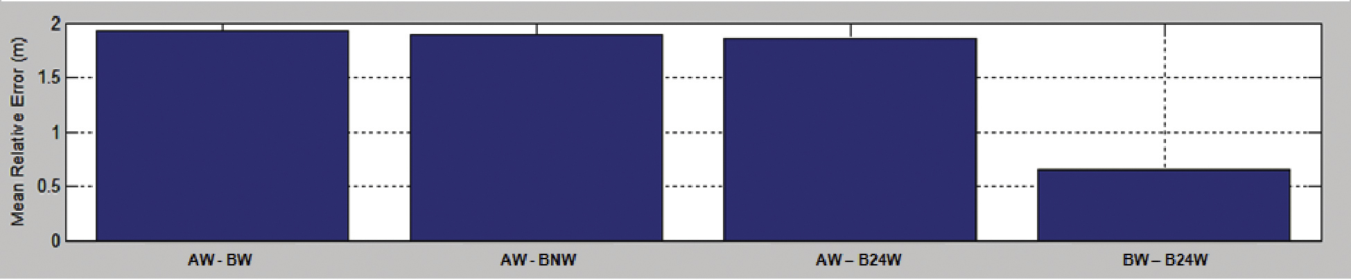
The relative accuracy with mixed receiver types or configurations was also estimated. With r
espect to receiver type mixes, the Type A receiver from vehicle 1 was used with the three Type B receivers in vehicle 2, yielding three combinations as AW–BW, AW–BNW, and AW–B24W. Mean error statistics for these three combinations and the combination of BW from vehicle 1 and B24W from the second vehicle are shown in Figure 3C. In comparison to the same type receiver pairing, this shows much larger mean errors. For instance, for all AW receiver mixes, the mean relative error is around 2 meters. Therefore, it is fair to conclude that error characteristics and modeling in the navigation solutions in receiver A and B are type-dependent, and they may not be compatible when a receiver mix is used. The BW–B24W combination does not show a significant increased mean error, indicating that the constellation difference in this test was not significant enough to result in an increased relative positioning error.
Figure 3A. Individual receiver absolute accuracy.Figure 3B. Relative accuracy with same receiver type.Figure 3C. Relative accuracy with receiver/configuration mix.
V2V Solution Availability
Availability statistics were generated for all accuracy categories (Which Road, Which Lane). At a more abstract level, solution availability statistics were also calculated for the DPOS and RTK methods. RTK solutions were defined as available whenever the software yielded a solution for that particular epoch. Data gaps in the RTK method could be caused by either communication failure due to, for example, a large truck entering the line of sight between vehicles, or one vehicle disappearing around a corner, or because insufficient observations from common satellites were available at the two vehicles. DPOS solutions, calculated in post-processing, were defined to be available whenever both receivers had observations from four or more satellites and were therefore able to calculate the necessary independent position solutions. While the two definitions of availability are not quite congruous, because only that for the RTK includes the possibility of communication failure, comparison of logs of data transmitted between the vehicles showed that out of approximately 45 hours of data, only 0.22 percent of missing RTK solutions could be attributed to failure of the DSRC link.
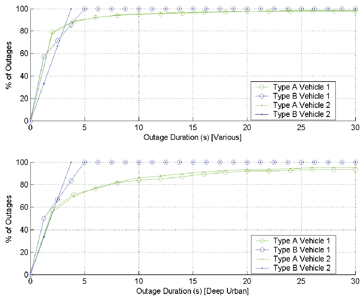
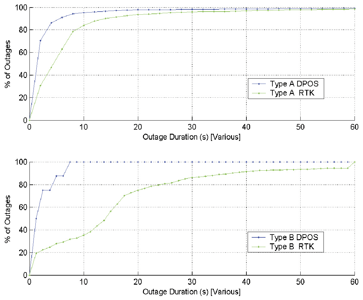
Figure 4 plots the distribution of GPS service outages observed by AW and BW receivers in individual vehicles in all of the test environments including deep urban. Here, as described for the DPOS method, an outage for a single receiver is identified on an epoch basis whenever the receiver has observations from less than four satellites. The total driving time included in this dataset is 45 hours and 4 minutes for each receiver. Figure 4 [deep urban] shows the same statistics for deep urban environment driving only, and this contains 1 hour and 40 minutes of driving for each receiver. The latter was selected specifically as this environment contained the most challenging conditions.
Figure 4. Distribution of GPS service outages for individual vehicles.
An important conclusion based on this data is that more than 98 percent of the individual vehicle-level service outages in the entire study lasted less than 30 seconds using any one of the receiver types. For the deep urban environment, 93 percent of the outages lasted less than 30 seconds. However, when using the high-sensitivity enabled Type B receivers, 100 percent of the outages lasted less than 5 seconds. No significant outage difference is seen between the observations from the same receiver type in the two vehicles.
GPS service availability for V2V applications was calculated using two approaches for the two relative positioning methods. For the DPOS method, individual vehicle service availabilities were time-synchronized in post-mission, and V2V DPOS solution availability was estimated. Figure 5 compares V2V solution outages using both receiver types and both relative positioning methods.
Figure 5. Distribution of GPS service outages for V2V applications.
The DPOS method yields better solution availability statistics than RTK. With both receiver types, more than 95 percent of DPOS solution outages are less than 10 seconds. With the RTK method, relatively longer outages were observed, especially for Type B receivers. With Type A receivers, the difference is only significant for outages shorter than 30 seconds. For Type B receivers, larger percentages of longer RTK outages were observed; this can be potentially attributed to poor carrier-phase tracking loop performance of these receivers and the impact on RTK.
Using GNSS Data
We anticipated performance issues arising from receiver type and configuration incompatibilities going into the prototype development effort. We identified use of raw GPS measurements instead of the DPOS method as one method to overcome this limitation, as the differencing techniques with measurement data guarantees correlated error cancellation. This was one reason to include the RTK capability in the prototype system. Therefore, confirming the fact that use of raw measurements eliminates the receiver type and configuration-related incompatibilities was a major goal of the study.
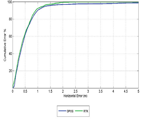
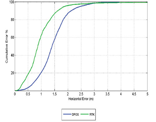
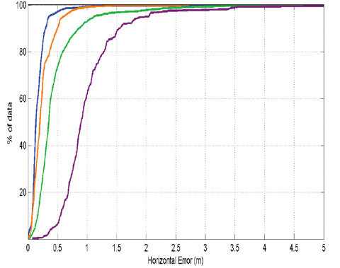
As discussed earlier, V2V relative position solutions using RTK were logged in real time as a part of the test setup. We compared these real-time RTK solutions and the DPOS solutions estimated in post-mission for all datasets. Figure 6 shows three cumulative probability distribution (CDF) plots generated using RTK and DPOS accuracy data from a freeway test dataset. The first CDF plot (left) shows the comparison of accuracy when both vehicles use Type A receivers with RTK and DPOS methods. The second CDF plot (center) shows the same CDFs when both vehicles use the Type B receivers. The third shows the DPOS and RTK accuracy CDFs when vehicle 1 uses Type A receiver and the other uses Type B receiver.
Figure 6 demonstrates that if higher quality GPS receivers similar to Type A are used in both vehicles, both RTK and DPOS methods would provide a solution of better than Which Lane accuracy more than 90 percent of the time. However, if Type B receivers are used, a solution with similar accuracy will only be available 60 percent of the time if the DPOS method is used for relative positioning of the vehicles. If the RTK method is used, this availability can be increased up to 90 percent.
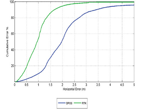
The performance difference between the two methods becomes even more prominent when the two vehicles use a mix of receiver types. In the right-most CDF of Figure 6, a solution with Which Lane accuracy is only available 30 percent of the time if DPOS method is used with the mixed receiver configuration. The RTK solution availability still remains around 90 percent even with the mixed configuration. This confirms that use of measurement data eliminates some of the limitations associated with the DPOS method.
Comparison of only the RTK performance between all three CDFs in Figure 6 shows that RTK V2V performance is only limited by the worst-performing receiver in the receiver combination. Out of the three CDFs, the middle (both vehicles using Type B) and the right (Type A and B mix) CDFs have almost identical RTK performance curves. Given that the RTK curve with both using Type A receivers shows much better performance, it is fair to conclude that in the mixed-receiver case, the RTK curve is limited by the performance of th
e Type B receiver. Figure 6 also shows that at Which Road accuracy, all receiver combinations and both processing methods yield almost identical performance.
Figure 6A. Comparison of V2V solutions using RTK and DPOS methods.Figure 6B. Comparison of V2V solutions using RTK and DPOS methods.Figure 6C. Comparison of V2V solutions using RTK and DPOS methods.
Other Approaches
Given that carrier-phase measurements are subject to cycle slips in some road environments, we ran a test using code measurements only in relative mode, using selected data sets collected on a mountainous highway. Only common satellites were used. Given that code measurements are not affected by a loss of phase lock, such a solution is more robust, but is subject to code noise and multipath. The RMS horizontal position differences between these solutions and the reference inter-vehicle separations were 25 centimeters and 1 meter for receiver Types A and B, respectively. Both receiver types meet the Where-in-Lane requirement in this test. Type A, with its low code noise and excellent code multipath-reduction capability, has a clear advantage.
Such an approach would represent a compromise between the DPOS and RTK approaches. Its advantage over the RTK approach is a lower data transmission-rate requirement, while that over the DPOS approach is the use of common satellites only. The latter is quite significant, since low-elevation satellites contribute the most to horizontal position solutions, but their measurements are affected more by atmospheric transmission errors that are most effectively removed in differential mode on a satellite-by-satellite basis.
V2V Operation with V2I
While infrastructure support can almost always improve the performance of other V2X applications, it can pose a challenge for positioning when such coverage is not continuous. The complication arises as a result of vehicles transitioning in and out of V2I coverage areas. V2I systems are highly likely to include GNSS augmentation capability so that vehicles within a coverage area benefit from better positioning capability. However, when vehicles transition from standard (V2V) operation mode to a V2I enhanced mode, some effects in the vehicle position domain can pose potential challenges for DPOS-based V2V.
The field study included test scenarios with limited V2I coverage in different driving environments: all of those described above with the exceptions of deep urban and mountains. In deployment, the infrastructure points (IPs) would broadcast aiding information to the vehicles within their coverage area, allowing real-time calculations. In the field study, in which the role of the IP was filled by a stationary high-grade receiver with a tripod-mounted antenna, all V2I estimates of the IVV were calculated using post-processing. Further, V2I estimates of the IVV were only calculated when at least one of the vehicles was within the coverage area of the IP, here chosen to be a circle of radius 300 meters centered at the IP. This range was chosen since it is the nominal effective range of the DSRC link.
The location of the IP, that is, the phase center of the stationary antenna, was determined using commercial RTK network software with additional stations at precise locations on the rooftop of a building at the University of Calgary. The estimated accuracy of this position was 5 millimeters (1 sigma). The distances of the vehicles from the IP, used to indicate when the vehicles transitioned into and out of the IP coverage area, were determined using the GPS/INS reference trajectories. In post-processing, once a vehicle was identified as having entered the IP coverage area, commercial RTK software was used to estimate the position of the vehicle, using the IP as base and each of the test receivers on that vehicle as rovers. The IVV was then calculated using the difference of the positions of the two vehicles. Thus, the V2I estimate of the IVV was determined using what is essentially the DPOS method with stationary base RTK-indicated vehicular positions, instead of the less accurate single-point GPS position solutions. When only one vehicle was within the coverage area, single-point solutions were used for the distal vehicle, resulting in a solution called V2I-S.
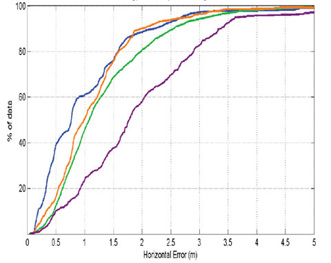
Figure 7 shows two sets of CDFs generated to illustrate the V2V positioning accuracy with V2I capability. The left plot corresponds to AW–AW receiver combination, and the right plot corresponds to the BW–BW combination. Each plot includes four curves. One pair of curves shows the V2V positioning accuracy without V2I, which includes performance when using the DPOS method (green) and another when using RTK (blue). The second pair shows the accuracy of the V2I and V2I-S estimates.
The most striking observation from Figure 7 is the separation of the V2I-S case from others for both receiver combinations (purple). It shows much worse positioning accuracy compared to the other three curves. For instance, using a BW–BW pair, the system will meet the Which Lane accuracy requirement around 80 percent of the time for either DPOS or RTK V2V without V2I support. However, when V2I coverage is available to only one vehicle, the V2I-S case, the accuracy requirement is only met at 40 percent confidence.
Figure 7A. Average relative positioning accuracy as a function of V2I positioning modes (orange V2I; green DPOS; blue RTK; purple V2I-S).Figure 7B. Average relative positioning accuracy as a function of V2I positioning modes (orange V2I; green DPOS; blue RTK; purple V2I-S).
Thus, system accuracy performance degrades when vehicles are operating in DPOS mode and are transitioning in and out of the V2I zones. This is because the V2I-S estimate is the difference of an accurate position solution for the vehicle within the coverage zone, and a potentially inaccurate single-point solution for the one outside the coverage zone. The beneficial cancellation of similar errors that occurs for DPOS estimates (using similar receivers and with common satellite observations) does not occur for V2I-S.
Potential solutions to this problem include using a V2I method of IVV calculation that is not dependent on the estimated position alone (that is, use RTK or other measurement-based methods as opposed to DPOS), or using a position-mode indicator with the DPOS mode such that a DPOS-based V2V solution is only generated when both vehicles are operating in the same mode (that is, V2I). However, the latter does not provide a remedy for the complications when the two vehicles are operating in two different modes. One could also consider a variation of the latter method whereby a V2I-augmented position and a non-augmented position is maintained by each vehicle, such that one of them could be used to generated a mode-matched DPOS V2V solution for a given sender.
Recommendations
These extensive trials provided valuable data demonstrating technical challenges associated with V2X positioning.
Error characteristics and modeling in the navigation solutions in receivers A and B are type-dependent, and they may not be compatible when a receiver mix is used with the DPOS mode. This is very likely to be the case for many other commercial receivers. Therefore, it is important to develop receiver hardware and software minimum-performance standards that define acceptable performance for measurement quality, satellite tracking and selection criteria, reliability estimates, navigation-solution parameters, and other such indicators.
Findings with RTK confirm the fact that use of measurement data eliminates some of the limitations associated with the DPOS method. While RTK is the most demanding raw data-based method in terms of processin
g requirements and OTA data needs, the study also conducted limited investigation on other methods that use raw code data and are less resource-intensive, and at the same time better performing than DPOS. Such an approach would represent a compromise between the DPOS and RTK approaches.
An important conclusion based on this data is that more than 98 percent of the individual vehicle-level service outages in the entire study lasted less than 30 seconds using any one of the receiver types. For the deep urban environment, 93 percent of the outages were less than 30 seconds. These statistics are useful for future research on suitable GNSS augmentation methods.
System accuracy performance degrades when vehicles operate in DPOS mode and transition in and out of the V2I zones. Potential solutions should be incorporated into the systems to take care of these limitations.
Acknowledgments
The authors thank the Crash Avoidance Metrics Partnership Vehicle Safety Communications-Applications team, in particular the Vehicle Positioning Technology Development team, for input. This work was conducted as a part of a CAMP VSC-A project under a cooperative agreement with the U.S. DOT.
CHAMINDA BASNYAKE is a senior research engineer at General Motors Global Research and Development and GNSS technology expert for GM OnStar. He leads GNSS-based vehicle navigation technology R&D efforts at GM and holds a Ph.D. in geomatics engineering from the University of Calgary.
TOM WILLIAMS is a postdoctoral researcher in the PLAN group in the Department of Geomatics Engineering at the University of Calgary.
PAUL ALVES is a Calgary-based geomatics consultant specializing in RTK. He obtained his doctorate from the University of Calgary.
GERARD LACHAPELLE holds an iCORE/CRC Chair in Wireless Location and heads the PLAN Group in the Department of Geomatics Engineering at the University of Calgary.
The Japan Aerospace Exploration Agency (JAXA) has controlled the orbit of the first quasi-zenith satellite system (QZSS) satellite, Michibiki. JAXA inserted Michibiki into the quasi-zenith orbit from the drift orbit starting on Sept. 21. The final orbit control operation was performed for about 50 seconds from 6:28 a.m. on Sept. 27 JST (Japan Standard Time).
After the operation, JAXA confirmed that the satellite was successfully injected into its preordained quasi-zenith orbit with its center longitude of about 135 degrees through the orbit calculation. The calculation results are as follows.
Michibiki was launched from the Tanegashima Space Center at 8:17 p.m. JST on Sept. 11.
JAXA will carry out the initial functional verification of the onboard mission devices in cooperation with organizations that will perform technological verifications for about three months. These organizations include the Geospatial Information Authority of Japan, the National Institute of Advanced Industrial Science and Technology, the National Institute of Information and Communications Technology, the Electronic Navigation Research Institute, and the Satellite Positioning Research and Application Center.
JAXA provided these definitions of drift and quasi-zenith orbit:
Drift orbit: The last step orbit prior to the quasi-zenith orbit. The orbit altitude and inclination (angle against the equator) are equal to those of the quasi-zenith orbit, but the longitude of the center of the figure-8 orbit is not above Japan. After being injected into the drift orbit, it will take a few days to maneuver the satellite to have its figure-8 center above Japan, thus it will ultimately fly in the quasi-zenith orbit.
Quasi-zenith orbit: While the quasi-zenith orbit has the same orbit period of 23 hours and 56 minutes as the geostationary orbit, it can let a satellite stay over Japan longer by taking an elliptical orbit with higher altitude above Japan and flying in a figure-8 orbit.
Global Positioning System experts from Air Force Space Command and the Space and Missile Systems Center will hold a media roundtable teleconference tomorrow, September 24, at 2:30 p.m. Mountain Time (4:30 p.m. Eastern Time) to discuss the recent GAO report titled “Global Positioning System: Challenges in Sustaining and Upgrading Capabilities Persist.” Colonel David Buckman, AFSPC command lead for positioning, navigation and timing, and Colonel Bernard Gruber, commander of the Global Positioning System Wing at Los Angeles Air Force Base, will participate in the teleconference.
Air Force Space Command, which has responsibility for sustaining and maintaining the Global Positioning System, feels that the GAO report is overly pessimistic and doesn’t adequately acknowledge what AFSPC has done to address constellation sustainment, according to a press release issued from the Air Force, Peterson Air Force Base, Colorado. “The Air Force has created the largest, most accurate constellation, with the greatest capability, in the history of GPS, with 31 operational satellites currently on orbit,” stated the press release. “This is well above the 24 minimum satellites needed for a full constellation and to meet constellation performance standards. Since 1995, GPS has never failed to exceed performance standards.”
The release continued, “AFSPC is working to mitigate the challenges identified by the GAO through a number of activities, including: applying a ‘back-to-basics’ approach to acquisition, continuing to identify additional ways to maximize the life of our operational satellites, implementing robust mission assurance processes, and transforming our launch enterprise.”
The first GPS IIF satellite completed on-orbit testing and checkout and was set operational on August 26 as planned, the Air Force said, The GPS IIF program is ready for full rate production and continues to build confidence in its production line. Through the institution of robust mission assurance processes, AFSPC is confident in the future of the GPS IIF program.
The follow-on program, GPS IIIA, recently completed critical design review, two months ahead of schedule, the Air Force said. “AFSPC is optimistic that its ‘back-to-basics’ approach, including stable requirements, mature technologies, and more government oversight, will ensure a successful program, providing the GPS IIIA and its ground segment, OCX, within a timeframe that maintains a robust GPS constellation and supports GPS users.”
At the Civil GPS Service Interface Committee meeting in Portland, Oregon, on Monday, Sergey Revnivykh, Deputy Director General of Roscosmos’s Central Research Institute of Machine Building reported on the status and future of GLONASS.
He provided a number of previously unpublished details on the present constellation and how it will be augmented in the future.
The present constellation officially has two reserve satellites, GLONASS 714 and 726. Revnivykh stated that neither of these satellites would ever be brought back to active service. 714 was a flight-test satellite, apparently, and 726 had a failure of its navigation payload. Rather than being possible replacement satellites, these vehicles are being used to train the ground team to operate spare satellites in a full or nearly full constellation.
GLONASS 727, in orbital slot 3, which was taken out of service on 8 September 2010 has also had a failure of its navigation payload and will not be returning to service. About 11 more GLONASS-M satellites will be launched by the end of 2012.
Revnivykh announced that there will be two versions of the new GLONASS-K satellites: GLONASS-K1 and GLONASS-K2. GLONASS-K1 satellites will have a 10-year design life and a daily clock stability of 5 ´ 10-14. The first GLONASS-K1 satellite will be launched this December from the Plesetsk Cosmodrome about 800 km north of Moscow. This will be the first launch of a GLONASS satellite from other than the Baikonur Cosmodrome. Only one more GLONASS-K1 satellite will be built and launched after that. The K1 satellites will test an open service CDMA signal on the GLONASS L3 frequency in the 1205 MHz band. When asked when the specific structure of the CDMA signal would be announced, Revnivykh said he didn’t know.
A completely new design, GLONASS-K2, will start launching in 2013. GLONASS-K2 satellites will have a 10-year design life and a clock stability of 1 ´ 10-14. Besides the CDMA signals on L3, CDMA signals will also be transmitted on L1 and L2. The GLONASS-K satellites will transmit the legacy FDMA satellites in addition to the CDMA signals.
A modernized GLONASS-K satellite, GLONASS-KM, for launch after 2015 is now under study. In addition to transmitting legacy FDMA signals on L1 and L2 and CDMA signals on L1, L2, and L3, CDMA signals may also be transmitted on the GPS L5 frequency at 1176.45 MHz. Also being studied is an alternative to the present three-plane, equally spaced satellite constellation. A different constellation design would be possible using CDMA signals. Such a move would require that the legacy FDMA signals be switched off. Revnivykh stated that any such move would require at least 10-years’ advance notice.
The design characteristics of the various generations of GLONASS satellites are shown in Figure 1, taken from Revnivykh’s presentation.
Figure 1. The GLONASS satellite generations through GLONASS-K2.
The signals that will be transmitted by the future generations of GLONASS satellites as well as those transmitted by the initial GLONASS satellites and the GLONASS-M satellites now on orbit are shown in Figure 2.
Figure 2. Signals transmitted by the different generations of GLONASS satellites. OF = open-access FDMA, SF = special (military) FDMA, OC = open-access CDMA, OCM = open-access CDMA modernized.
Revnivykh also spoke on the satellite-based augmentation system, SDCM (System for Differential Correction and Monitoring), under development. Correction and integrity data will be transmitted by Luch geostationary communication satellites now under development. Luch 5A, to be launched in 2011 and positioned at 16°W longitude and Luch 5B, to be launched in 2012 and positioned at 95°E longitude, will transmit signals on an L1 frequency. Luch 4, to be launched in 2013 and positioned at 167°E longitude, will transmit on two frequencies. The three satellites will provide almost global coverage. The satellite payloads are under development.
According to Revnivykh, the SDCM will make use of 12 monitor stations currently in operation in Russia and one in Antarctica at Russia’s Bellingshausen research station. However, the SDCM website indicates only 10 Russian stations currently in the test network. Eight more monitor stations will be added in Russia and five more outside Russia. Revnivykh showed a map revealing the locations of the additional overseas stations as Cuba, Brazil, Vietnam, Australia, and an additional station in Antarctica. It is not intended, at least initially, that these stations would be used in generating the orbit and clock data broadcast by the GLONASS satellites themselves.
And finally, Revnivykh stated that a GLONASS performance document will be released in the 2012-2013 time frame.
Launch of the first Quasi-Zentih Satellite System (QZSS) satellite, dubbed Michibiki, took place Saturday, September 11, at 11:17:00 UTC from the Tanegashima Space Center in Japan. At 28 minutes and 27 seconds after liftoff, Michibiki was separated from the launch rocket, H-IIA Launch Vehicle No. 18, according to Mitsubishi Heavy Industries, Ltd. and the Japan Aerospace Exploration Agency (JAXA).
JAXA performed the third apogee engine firing (AEF) for about 7 minutes from 12:21 p.m. on September 14
(Japan Standard Time, JST) by sending commands from the Okinawa station in Japan. Telemetry sent from the satellite confirms the third burn was a success. The satellite is in good health.
Another video can be viewed here. Below is an image of the ground track of the new orbit after the third AEF. Another two AEFs followed by thruster firings are required before the final orbit is obtained. Altogether the process is expected to take about two weeks.
As today’s handsets and consumer devices become more sophisticated, manufacturers continue to incorporate more and more functionality into a small and sleek form factor. Today’s range of smartphones incorporate voice and data transceivers, GPS, Bluetooth, Wi-Fi, cameras, music, touchscreen interfaces, compasses, motion sensors, cameras, storage cards, and many other technologies. Free turn-by-turn navigation services, such as offered on Google Android phones and iPhones, have created a compelling reason for many of us to own a GPS-equipped smartphone.
The pressure on manufacturers to integrate so many functions into one small printed circuit board has fueled a race among semiconductor suppliers to offer new solutions combining GPS and wireless connectivity. Phones that are small and comfortable to hold mean less and less space available for the internal electronics. Large screen sizes and the trend to thinner and thinner devices means smaller, less efficient antennas, placing pressure on chip designers to improve integrated circuit (IC) performance to make up for antenna constraints.
Finally, cost competition in these markets is intense, as operators compete to bring more users online.
These forces have shaped several changes in the wireless semiconductors found in new smartphones. Three important enabling technologies are:
reduced-geometry semiconductor technologies,
wafer-scale packaging, and
combo chip integration.
Let’s look at the trends in each area.
Semiconductor transistor sizes have been shrinking for decades. GPS processors in the market today use transistor geometries with gate widths of 0.18 micrometers, 0.13 micrometers, 90 nanometers (nm), and 65 nm, the latter showing up in the newest handsets on the market. 40-nm-based ICs have been announced as well, and will find their way into the market in the next year or two.
Each generation of technology offers a 50–100 percent increase in density for pure digital circuits. This so-called shrink has allowed designers to both reduce the size of chips and to pack in more performance — in GPS chips this usually means more tracking channels and more correlators for faster signal search. The area for non-digital circuits such as the radio receiver in a GPS has not been shrinking as fast as the digital portion. This had led to changes in architecture, with more and more functions going digital. Examples include digital band-shaping filters, digital gain adjustment, and sigma-delta analog- to-digital converters.
Wafer-scale packaging has moved into the mainstream for GPS and other wireless ICs. Traditional ball-grid array (BGA) packaging requires placing a semiconductor die on a substrate. The substrate carries the balls (pins) and some interconnects, and the semiconductor die is connected to the substrate via wire bonds. For small ICs the overall package size may be 50 percent larger than the die itself, because of overhead of the space needed for wire bonds.
By contrast, wafer-level ball grid array (WLBGA) packaging yields a finished packaged part with the same dimensions as the underlying die. Wire bonds are not used; a redistribution layer (RDL) is bonded to the silicon wafers and carries interconnections from the silicon to the balls. This type of packaging yields the smallest possible board footprint. It also places strict limitations on the number of package pins, since the pins must all fit under the chip and cannot be spaced too closely, due to board manufacturing constraints. Often designers struggle to provide the features customers seek while abiding by package pin-count limitations. Pins are shared or multiplexed to preserve flexibility.
Combo-chip integration offers the ultimate solution for small size. A single IC with multiple functions will almost always be considerably smaller than several ICs on a printed board. The last two years have seen the introduction of several combo ICs containing GPS, including the Broadcom’s BCM2075 Bluetooth-FM-GPS combo IC. Combo ICs like this allow manufacturers to build cellular handsets that would be difficult or impossible to create using discrete chip sets. Since GPS, FM, and Bluetooth have become standard features across many product lines, manufacturers not only benefit from small size but also economies of scale, designing a single part into dozens of devices.
The benefits of combo ICs are easy to understand, but making these devices brings unique challenges. First and foremost, these ICs are wireless devices containing multiple sensitive radios, where every fraction of a decibel of performance counts. With few exceptions, handset manufacturers and their wireless operator customers are not willing to sacrifice radio performance in their quest for miniaturization and cost reduction. Each function on the wireless combo IC must perform as well as its counterpart function in a stand-alone IC.
However, in a combo IC the radios are at most a few millimeters apart from each other. Designing for this type of integration requires engineering attention at multiple stages of the design. Up front, during the system engineering phase, component specifications must be set that minimize interference between radio subsystems, considering not just the radios on the combo IC but the influence of other radios in a handset as well. For example, in setting the specification for the second-order intercept point of the GPS receiver, system engineers must consider the fact that transmissions in 825 MHz cellular band can mix with Bluetooth transmissions at 2400 MHz to yield an intermodulation product at 1575 MHz, right in the middle of the GPS receive band. Designers also choose clock frequencies to avoid interference; for example, a GPS baseband processor that clocks at 100 MHz might be changed to 75 MHz to avoid the FM receive band. These are just a couple of examples of the many scenarios and considerations that must be examined early in the design process.
Once the system engineer has done his or her job, the next level of interference mitigation falls on the analog designers. They choose where to place circuits, how to structure the semiconductor layers, how to drive and load interconnects, and how to properly filter supply voltages to avoid undesired interactions. Keeping spurious products off local oscillator signals is a key challenge. GPS receivers have 100 dB or more of gain to amplify very weak GPS signals to a usable level. Due to this high gain, even a tiny spurious product on a local oscillator can have the effect of tuning in an undesired cellular transmitter. For example, a spurious product offset 135 MHz will tune a cellular transmitter at 1710 MHz down to 1575 MHz, again right in the middle of the GPS band. Avoiding these interactions requires experienced designers who can anticipate complex issues. Mistakes can be costly, with each mask for each IC iteration going into seven figures.
As the challenges of combo ICs are overcome, it’s likely the future will bring even more in the way of wireless technology integration. This in turn will provide even more opportunities for GPS to penetrate a broader set of handsets and cellular devices, making this exciting technology available to more consumers every day.
CHARLES ABRAHAM is senior director of engineering for the GPS Business Unit at Broadcom, which he joined via acquisition of Global Locate, a company he co-founded in 2000. Previously, he worked at Ashtech, Magellan, Trimble, and Hughes Electronics.
By John Nielsen, Ali Broumandan, and Gérard Lachapelle
Ubiquitous adoption of and reliance upon GPS makes national and commercial infrastructures increasingly vulnerable to attack by criminals, terrorists, or hackers. Some GNSS signals such as GPS P(Y) and M-code, GLONASS P-code, and Galileo’s Public Regulated Service have been encrypted to deny unauthorized access; however, the security threat of corruption of civilian GNSS signals increases constantly and remains an unsolved problem. We present here an efficient approach for the detection and mitigation of spoofed GNSS signals, as a proposed countermeasure to add to the existing system.
Current methods to protect GPS civilian receivers from spoofing signals are based on the cross-check with available internal/external information such as predictable characteristics of the navigation data bits or correlation with ancillary inertial-based sensors; alternately, a joint process of signals received at two separate locations based on processing the P(Y)-code.
The authentic GNSS signal sourced from a satellite space vehicle (SV) is very weak at the receiver’s location and is therefore vulnerable to hostile jamming based on narrowband noise radiation at a modest power level. As the GNSS frequency band is known to the jammer, the effectiveness of the latter is easily optimized by confining radiation to within the GNSS signal band. The jammed GNSS receiver is denied position or time estimates which can be critical to the mission. While noise jamming of the GNSS receiver is a threat, the user is easily aware of its existence and characteristics. The worst case is that GNSS-based navigation is denied.
A more significant jamming threat currently emerging is that of the spoofing jammer where bogus signals are transmitted from the jammer that emulate authentic GNSS signals. This is done with multiple SV signals in a coordinated fashion to synthesize a plausible navigation solution to the GNSS receiver. There are several means of detecting such spoofing jammers, such as amplitude discrimination, time-of-arrival discrimination, consistency of navigation inertial measurement unit (IMU) cross-check, polarization discrimination, angle-of-arrival (AOA) discrimination, and cryptographic authentication.
Among these authentication approaches, the AOA discriminator and spatial processing have been addressed and utilized widely to recognize and mitigate hostile attacks. We focus here on the antenna-array processing problem in the context of spoofing detection, with considerations to the pros and cons of the AOA discriminator for handheld GNSS receivers.
An exploitable weakness of the spoofing jammer is that for practical deployment reasons, the spoofing signals generally come from a common transmitter source. Hence, a single jamming antenna sources the spoofing signals simultaneously. This results in a means of possible discrimination between the real and bogus GNSS signals, as the authentic GNSS signals will emanate from known bearings distributed across the hemisphere.
Furthermore, the bearing of the jammer as seen from the GNSS receiver will be different than the bearing to any of the tracked GNSS satellites or space vehicles (SV). This immediately sets up some opportunities for the receiver to reject the spoofing jamming signals. Processing can be built into the receiver that estimates the bearing of each SV signal. Note that the relative bearings of the GNSS signals are sufficient in this case, as the bogus signals will all have a common bearing while the authentic GNSS signals will always be at different bearings.
If the receiver comprises multiple antennas that have an unobstructed line of sight (LOS) to the SVs, then there are possibilities of spoofing detection based on the common bearing of the received GNSS signals and eliminating all the jammer signals simultaneously by appropriate combining of the receiver antennas to form a pattern null coincident with the jammer bearing.
Unfortunately, the AOA discrimination will not be an option if the jammer signal or authentic signals are subjected to spatial multipath fading. In this case, the jammer and individual SV signals will come in from several random bearings simultaneously. Furthermore, if the GNSS receiver is constrained by the form factor of a small handset device, an antenna array will not be an option. As the carrier wavelength of GNSS signals is on the order of 20 to 25 centimeters, at most two antennas can be considered for the handset receiver, which can be viewed as an interferometer with some ability of relative signal-bearing estimation as well as nulling at specific bearings.
However, such an antenna pair is not well represented by independent isotropic field sampling nodes, but will be significantly coupled and strongly influenced by the arbitrary orientation that the user imposes. Hence, the handset antenna is poorly suited for discrimination of the spoofing signal based on bearing. Furthermore, handheld receivers are typically used in areas of multipath or foliage attenuation, and therefore the SV signal bearing is random with significant variations.
As we discuss here, effective spoofing detection is still possible for a single antenna GNSS receiver based on the differing spatial correlation of the spoofing and authentic signals in the proximity of the receiver antenna. The basic assumption is that the antenna will be spatially moved while collecting GNSS signal snapshots. Hence, the moving antenna generates a signal snapshot output similar to that of a synthetic array (SA), which, under some additional constraints, can provide an effective means of detecting the source of the GNSS signals from a spoofing jammer or from an authentic set of SVs.
We assume here an arbitrary antenna trajectory with the spoofing and authentic signals subjected to random spatial multipath fading. The processing will be based on exploiting the difference in the spatial correlation of the spoofing and the authentic signals.
Spoofing Detection Principle
Consider a GNSS handset receiver (Figure 1) consisting of a single antenna that is spatially translated in time along an arbitrary trajectory as the signal is processed by the GNSS receiver. There are L authentic GNSS SV signals visible to the receiver, along with a jammer source that transmits spoofing replicas of the same Lauthentic signals.
FIGURE 1. GNSS receiver with a single antenna and 2L parallel despreading channels simultaneously providing channel gain estimates of L authentic and L spoofing signals as the antenna is moved along an arbitrary spatial trajectory.
It is assumed that the number of spoofed signals range from 1 to L, which are coordinated such that they correspond to a realistic navigation solution at the output of the receiver processing. The code delay and Doppler associated with the spoofing signals will typically be different than those of the authentic signal. The basic technique of coordinated spoofing jamming is to present the receiver with a set of L signals that appear to be sufficiently authentic such that the spoofing and authentic signal sets are indistinguishable. Then the spoofing signals separate slowly in terms of code delay and Doppler such that the navigation solution corresponding to the L spoofing signals will pull away from the authentic navigation solution.
The focus herein is on methods where the authenticity of the L tracked GNSS signals can be tested directly by the standalone receiver and then selected for the navigation processing. This is in contrast with other methods where the received signals are transmitted back to a communication command center for verification of authenticity. The consideration here is on the binary detection problem of assessing if each of the 2L potential signals is authenti
c or generated by a spoofing source. This decision is based on observations of the potential 2L GNSS signals as the antenna is spatially moved through the trajectory.
The complex baseband signal at the output of the antenna, denoted by r(t), can be expressed as
where i is the GNSS signal index, the superscripts A and J indicate authentic and jamming signals respectively, p(t) shows the physical position vector of the moving antenna phase center relative to a stationary spatial coordinate system, ΛAi(p(t),t) and ΛJi(p(t),t) give the channel gain for the authentic and the spoofing signals of the ith SV at time t and position p, ci(t) is the PN coding modulation of ith GNSS signal, πAi and πJi are the code delay of ith PN sequence corresponding to the authentic and the spoofing sources respectively, fDiA and fDiJ are the Doppler frequency of the ith authentic and the spoofing signals and w(t) represents the complex baseband of additive noise of receiver antenna. For convenience, it is assumed that the signal index iε[1, 2,…,L] is the same for the spoofing and authentic GNSS signals. The spoofer being aware of which signals are potentially visible to the receiver will transmit up to L different spoofing signals out of this set.
Another simplification that is implied by Equation 1 is that the message coding has been ignored, which is justifiable as the GNSS signals are being tracked such that the message symbol modulation can be assumed to be removable by the receiver by some ancillary process that is not of interest in the present context. The objective of the receiver despreading operation is to isolate the channel gains ΛA(p(t),t) ΛJ(p(t),t), which are raw observables used in the subsequent detection algorithm.
It is assumed that the GNSS receiver is in a signal tracking state. Hence, it is assumed that the data coding, code phase of the spreading signal and Doppler are known inputs in the despreading operation. The two outcomes of the ith despreading channel for authentic and jamming signals are denoted as riA(t) and rkJ(t) respectively, as shown in Figure 1. This notation is used for convenience and not to imply that the receiver has knowledge of which of the pair of GNSS signals corresponds to the authentic or spoofer cases. The receiver processing will test each signal for authenticity to select the set of L signals that are passed to the navigation estimator.
The despread signals riA(t) and rkJ(t) are collected over a snapshot interval of tε[0,T]. As the notation is simplified if discrete samples are considered, this interval is divided into M subintervals each of duration ΔT such that the mth subinterval extends over the interval of [(m−1)ΔT,mΔT]for mε[1,,2,…,M]. The collection of signal over the first and mth subintervals is illustrated in Figure 2. ΔT is considered to be sufficiently small such that ΛAi(p(t),t) or ΛJk(p(t),t) is approximately constant over this interval leading a set of M discrete samples for each despreading output. From this the vectors form of channel gain sample and outputs of despreaders can be defined by
where ΛAi(p(mΔT),mΔT) and ΛJi(p(mΔT),mΔT) are the mth time sample of the ith despreader channel for the authentic and jamming GNSS signals.
Figure 2. Spatial sampling of the antenna trajectory into M subinterval segments.
Pairwise Correlation
The central tenet of the spoofing detection is that the array gain vector denoted here as the array manifold vector for the jammer signals ΛJ will be the same for all of the L spoofing signals while the array manifold vector for the authentic signals ΛA will be different for each of the L authentic signals. If the random antenna trajectory is of sufficient length, then the authentic signal array manifold vectors will be uncorrelated. On the other hand, as the jammer signals emerge from the same source they will all have the same array manifold vector regardless of the random antenna trajectory and also regardless of the spatial fading condition. This would indicate that a method of detecting that a spoofer is present to form the Mx2L matrix of all of the despreader output vectors denoted as r and given as
where it is assumed that M≥2L.
Basically what can be assumed is that, if there is a spoofer from a common source that transmits more than one GNSS signal simultaneously, there will be some residual spatial correlation of the observables of ΛJi with other despreader outputs of the receiver. Therefore, if operations of pairwise correlations of all of the 2L despreader outputs result in high correlation, there is a likelihood of the existence of spoofing signals. These pairwise correlations can also be used to distinguish spoofing from authentic signals. Note that even during the time when the spoofing and authentic signals have the same Doppler and code offset, the superposition manifold vector of ΛAi and ΛJi will be correlated with other spoofing manifold vectors. The pairwise correlation of the various spoofing signals can be quantified based on the standard numerical estimate of the correlation coefficient given as
where ri is the ith column vector of r defined in Equation 3, and the superscript H denotes the complex conjugate operator.
Toward Spoofing Detection
Figure 3 shows the spoofing attack detection and mitigation methodology:
The receiver starts with the acquisition process of a given GNSS code. If, for each PN sequence, there is more than one strong peak above the acquisition threshold, the system goes to an alert state and declares a potential spoofing attack. Then the receiver starts parallel tracking on each individual signal.
The outputs of the tracking pass to the discriminator to measure the correlation coefficient ρ among different PN sequences. As shown in Figure 3, if ρ is greater than a predefined threshold ϒ, the receiver goes to defensive mode. As the spoofer attempts to pull the tracking point off the authentic signals, the spoofer and authentic signals for a period of time will have approximately the same code offset and Doppler frequency. Hence, it may not be possib
le to detect more than one peak in the acquisition mode. However, after a while the spoofer tries to pull tracking mode off.
The outputs of the parallel tracking can be divided into two groups: the J group is the data set that is highly correlated, and the A group is the set that is uncorrelated. It is necessary that the receiver antenna trajectory be of sufficient length (a few tens of the carrier wavelengths) such that M is moderately large to provide a reasonable estimate of the pairwise correlation.
The A group will be constrained in size based on the number of observable satellites. Usually this is known, and L can be set. The receiver has control over this by setting the bank of despreaders. If an SV signal is known to be unobtainable due to its position in the sky, it is eliminated by the receiver. Hence the A group can be assumed to be constrained in size to L. There is the possibility that a spoofer will generate a signal that is clear, while the SV signal is obscured by shadowing obstacles. Hence a spoofing signal can inadvertently be placed in the A group. However, as this signal will be correlated with other signals in the J group, it can be transferred from the A to the J group.
When the spoofing navigation solution pulls sufficiently away from the authentic solution, then the navigation solution can create two solutions, one corresponding to the authentic signals and the other corresponding to the spoofing signals. At this stage, the despreading code delay and Doppler will change such that the authentic and spoofing signals (corresponding to the same GNSS signal) will appear to be orthogonal to each other.
Proper placement of the members in the J and A groups can be reassessed as the set of members in the A group should provide the minimum navigation solution variance. Hence, in general there will be a spoofing and authentic signal that corresponds to the GNSS signal of index i. If the spoofing signal in group J appears to have marginal correlation with its peer in group A and, when interchanged with its corresponding signal in group A, the latter generates a lower solution variance, then the exchange is confirmed.
Figure 3. Spoofing detection and mitigation methodology.
Experimental Measurements
We used two data collection scenarios in experiments of spoofing detection, based on utilizing a single antenna that is spatially translated, to demonstrate the practicality of spoofing-signal detection based on spatial signal correlation discrimination. In the first scenario, the spoofing measurements were conducted inside a modern three-story commercial building. The spoofing signals were generated by a hardware simulator (HWS) and radiated for a few minutes indoors, using a directional antenna pointing downward to affect only a small area of the building. The intention was to generate NLOS propagation conditions with significant multipath.
The second data collection scenario was based on measuring authentic GPS L1 C/A signals under open-sky conditions, in which case the authentic GPS signals are temporally highly correlated. At the particular instance of the spoofing and the authentic GPS signal measurement scenarios, the SVs were distributed as shown in Figure 4. The GPS receiver in both scenarios consisted of an active patch right-hand circular polarized (RHCP) antenna and a down-conversion channelizer receiver that sampled the raw complex baseband signal. The total data record was subsequently processed and consisted in acquiring the correlation peaks based on 20-millisecond coherent integration of the spoofing signals and in extracting the channel gains L as a function of time.
Figure 4. Skyplots of available satellites: a) spoofing signals from Spirent generator, b) authentic signals from rooftop antenna.
Figure 5 shows a plot of the samples of the magnitude of despreader outputs for the various SV signals generated by the spoofing jammer and authentic signals. The signal magnitudes in the spoofing case are obviously highly correlated as expected, since the jammer signals are all emanating from a common antenna. Also, the SNRs are moderately high such that the decorrelation due to the channel noise is not significant.
The pairwise correlation coefficient using Equation 4 are calculated for the measurement results represented in Figure 5 and tabulated in Table 1 and Table 2 for the spoofing and the authentic cases respectively. As evident, and expected, the correlations for the spoofing case are all very high. This is anticipated, as the spoofing signals all occupy the same frequency band with exception of small incidental shifts due to SV Doppler.
Figure 5. Normalized amplitude value of the signal amplitude for different PRNs: a) generated from the same antenna, b) Authentic GPS signals.TABLE 1. Correlation coefficient deter- mined for the set of spoofing signals.TABLE 2. Correlation coefficient deter- mined for the set of authentic signals.
Conclusions
Spoofing signals generated from a common source can be effectively detected using a synthetic array antenna. The key differentiating attribute exploited is that the spoofing signals emanating from a single source are spatially correlated while the authentic signals are not. The method works regardless of the severity of multipath that the spoofing or authentic signals may be subjected to. The receiver antenna trajectory can be random and does not have to be jointly estimated as part of the overall spoofing detection.
A patent is pending on this work.
Manufacturers
The experimental set-up used a Spirent GSS7700 simulator, National Instruments receiver (NI PXI-5600 down converter, and NI PXI-5142 digitizer modules), TECOM directional helical antennas as the transmitter antenna, and NovAtel GPS-701-GG as the receiver antenna.
JOHN NIELSEN is an associate professor at the University of Calgary.
ALI BROUMANDAN is a senior research associate in the Position Location And Navigation (PLAN) group at the University of Calgary. He obtained a Ph.D. in Geomatics Engineering from the University of Calgary in 2009.
GERARD LACHAPELLE holds an iCORE/CRC Chair in Wireless Location and heads the PLAN Group in the Department of Geomatics Engineering at the University of Calgary.
The first time I ever heard of the Magnavox Research Laboratory in Torrance, California, was in 1966, as a young engineer working at Hughes Aircraft. We were building large (46-foot diameter) ground stations for the Defense Satellite Communications System (DSCS). Magnavox was supplying the secret anti-jam modems used in the terminals.
Because of this, I also learned a little about spread-spectrum pseudo-noise (PN), something quite esoteric at the time and not taught in engineering school. I noticed a widespread respect for Magnavox from my colleagues who referred to the company and its equipment as “Magicbox.”
Within a year I had transferred to the Hughes division responsible for developing satellites. We were working on a study known as 621B, for using satellites for positioning. Our teammate for the study was Magnavox. That team was responsible for the payload signal design, for which the team chose PN as the modulation to provide for multiple access, ranging, data transmission, and anti-jam.
Before long, my boss decided to leave Hughes and go work for Magnavox. He took two of his systems engineers with him. I was one of them.
In1968, the U.S. Air Force could not yet sell the 621B concept as an Advanced Development Program, so instead opted to experiment and prove that PN modulation could be used to accurately measure a half-mile of cable. Hughes bowed out since there wasn’t any satellite procurement in the offing. Magnavox and the other 621B contractor, TRW, each took on the challenge of measuring the cable.
Where Hughes had been 10-deep in Ph.D.s in every discipline, Magnavox was 10-deep in PN experts, which I believe at that time was the world’s majority. Thus it was natural for the Air Force to ask them to continue, and develop a receiver to be used in the next phase of 621B. An inverted range was set up with four PN transmitters, and an aircraft with the receiver and a bottom antenna flew over them. The aircraft’s position was determined using the PN range measurements and the known locations of the transmitters. The data from that receiver, called the MX450, was used to help justify the Department of Defense (DoD) decision to proceed into the Advanced Development Phase of GPS. Some of the people who contributed to this were named in Dr. Brad Parkinson’s recent articles on the origins of GPS. During that time I was working on the next generation of spread-spectrum modems for the DSCS.
Magnavox went on to develop these PN satcom modems for all three services, and thus was a natural choice to develop the first military GPS receivers (known as X and Y sets and the first Manpack), as well as the first C/A receiver, the Z set, and the very first spaceborne receiver called GPSPAC.
As soon as we completed the first Manpack, I approached Col. Paul Weber, the Joint Program Office Army Deputy Program Manger, and asked if he would pose with the Manpack on his back for a brochure we wanted to produce to show to potential Army and Marine Corps users. He agreed, dressed in his combat uniform, and went with our photographer into the wild woods of San Pedro (near the Port of Los Angeles) for the picture shown in the brochure.
Magnavox also developed the military GPS Engineering Models in competition with Rockwell Collins. Magnavox lost the production contract to Rockwell Collins a year after I left to join IEC, now known as L-3 Communications.
Magnavox also pioneered commercial GPS sets for use in the marine and survey markets. Today, you will still find many of the original GPS user equipment developers still at it as consultants and engineers at Raytheon, Navcom, Trimble, IEC, and others. Perhaps our most famous alumni is Dr. Min Kao, the “min” of Garmin.
Len Jaconbson
LEN JACOBSON is a consultant to the GPS industry and has served as an expert witness in many legal proceedings involving GPS. He is the author of the book GNSS Markets and Applications, published in 2007, and is a longstanding member of this magazine’s Editorial Advisory Board.
I wish to second Jim Spilker’s comments in his recent letter to the editor regarding the two wonderful GPS history articles by Brad Parkinson. My endorsement of his comments also includes those about the origins of the L5 signal with reference to the 1999 paper by Spilker and Van Dierendonck, “Proposed New Civil GPS Signal at 1176.45 MHz.” Jim commented in the letter that “. . . . the work I did in designing the GPS L5 signal was performed as a gift to the U.S. Air Force, Federal Aviation Administration, and our country, . . .” It was a generous contribution, and I applaud it.
However, this leads me to comment on other very important but underreported gifts to L5 and subsequent signal developments. A small indication of the L5 contributions is given in the brief acknowledgement at the end of the referenced paper, “The authors wish to acknowledge the contributions of Dr. C.R. Cahn and Thomas Stansell in the selection of this signal.” It also is important to recognize that the L5 signal structure was formulated within an RTCA committee of mostly volunteers. Among other key participants, in addition to A.J., was Dr. Chris Hegarty.
The L5 signal design included several innovations which influenced subsequent development of modernized GPS signals and of signals for other GNSS. My ranking of the most important L5 innovations is:
Center frequency of 1176.45 MHz in an ARNS band
Two signal components, one with a data message and the other without (pilot signal)
Forward error correction (FEC) (first GPS use, borrowed from WAAS)
Overlay code to frame symbols and eliminate need for bit synchronization
CNAV message structure for better accuracy and more flexibility
The list doesn’t include the 10.23 MHz code clock rates or having two signals in phase quadrature, which were included in the first GPS satellite launched in 1978. The new center frequency was recommended by Karl Kovach (then with ARINC and now with Aerospace) and adopted before the signal design began, but it was central to the L5 purpose of having a civil signal in an ARNS band. This same center frequency also will be provided by Galileo and Compass, so it was a vital innovation. Although forward error correction had been adopted for WAAS, the first use on GPS was the L5 design. In one form or another, it too will be used on most if not all other GNSS signals.
The second and fourth innovations in the list above were contributed by Dr. Charlie Cahn with help and encouragement from Richard (Rich) Keegan and myself. Having a dataless or pilot signal provides a significant boost to performance and has been adopted for almost every subsequent GNSS signal. The problematic C/A bit synchronization process has been eliminated by the data symbol overlay code (or equivalent) in all subsequent signals. The CNAV message format was principally developed by Karl Kovach with significant help from Art Dorsey of Lockheed Martin.
In summary, Brad Parkinson helped memorialize many of the early “GPS Heroes” who made GPS what it is today. Other heroes have contributed to GPS modernization, and credit should be given where credit is due. Brad mentioned Charlie Cahn, one of my real heroes, who helped shape the 621B and early GPS signals and has continued to contribute in many ways. In addition to the very significant innovations mentioned above, Charlie was key to similar improvements made in the subsequent L2C, M-code, and L1C signal designs.
— Tom Stansell
Kauai, Hawaii
An Advisor Bids Farewell
Paul Cross
Many thanks for the kind invitation to GPS World’s Leadership Dinner. I have to decline as I won’t attend ION-GNSS this year. I will retire from University College London at the end of September. I don’t plan to remain active in the world of GNSS after my retirement so this would be a good time for me to step down from the Editorial Board. I’ve very much enjoyed my association with GPS World and have benefited enormously from it.
I wish you and the magazine continued success. You have come a long way over the past twenty years or so and you are now, and have been for some time, the premier source of news (and very useful gossip!) relating to GNSS worldwide. I don’t know anyone of any significance who doesn’t read GPS World every month. Your highly accessible technical articles have been of enormous help to many cohorts of students here at UCL, and all over the world.