Epson recently announced in a news release the launch of its Pro G7000-Series large venue projectors for simulators, mapping, digital signage and command centers.
New features include increased brightness and motorized lenses, uncompromising image quality, low total cost of ownership and $199 replacement lamps, Epson says. Eight models deliver up to 8,000 lumens of color brightness and 8,000 lumens of white brightness.
The series also features the world’s first zero-offset ultra short-throw lens with 0.35 throw ratio for space constrained venues and digital signage applications. The Pro G-Series will be on display at ISE 2016 in Amsterdam from Feb. 9–12 at Epson’s booth, No. 1-H90.
“The Epson Pro G-Series offers bright, brilliant images combined with advanced features, making them our best-selling large venue projectors,” said Phong Phanel, product manager of large venue projectors, Epson America Inc. “The new Pro G7000-Series raises the bar with higher brightness, 4K Enhancement resolution, new motorized lenses and advanced technology to captivate any audience, underscoring our commitment to delivering a broad portfolio of solutions to the large venue projector market.”
Epson projectors offer three times higher color brightness than competitive 1-chip DLP models to ensure vivid colorful images. The Pro G Series 3-chip 3LCD projectors are ideal for large venues, including events staging, auditoriums and sanctuaries.
The Epson Pro G7000-Series will be available in May starting at $3,799 MSRP. The projectors come with a three-year limited warranty with next business day replacement, including free shipping both ways7, and a 90-day limited lamp warranty.
The color brightness specification — measuring red, green and blue — published by the Society for Information Display (SID) allows consumers to compare projector color performance without conducting a side-by-side shootout.
From (L to R) John Palatiello, MAPPS executive Director; Jim Green; Mike Sitar and Michel Stanier of Optech Teledyne.
Teledyne Optech‘s ALTM Titan lidar sensor earned the 2015 Grand Award in the ninth annual MAPPS Geospatial Products and Services Excellence Awards, MAPPS recently announced in a news release. The awards ceremony was held Feb. 2 at the Green Valley Ranch in Henderson, Nev.
Teledyne was also presented with an award in the Technology Innovation category.
The company said in a news release that Titan is easy to handle in complex scenarios, such as acquiring three wavelengths simultaneously; incorporating a metric camera imbedded in the system; creating a sensor that fits in a 16-inch gyro-stabilized mount; and increasing the depth penetration of the bathymetric sensor. To achieve this, Vaughan, Ontario-based Teledyne Optech had to develop new fiber lasers and a triple wavelength receiver which allowed for the collection of bathymetric lidar, topographic lidar and multispectral lidar in one single sensor.
“Teledyne Optech’s ALTM Titan is a marvel in lidar engineering,” said Robert Burtch PS, CP, professor emeritus at Ferris State University in Big Rapids, Mich., and chairman of the panel of judges. “This development allows the collection of bathymetric lidar, topographic lidar and multispectral lidar in one single sensor.”
The MAPPS awards competition recognizes the professionalism, value, integrity and achievement that member firms have demonstrated in their projects and technology developments over the previous year.
MAPPS also honored winners in six technical categories.
Woolpert of Dayton, Ohio, was selected in the Photogrammetry/Elevation Data Generation category with the Little Bighorn Battlefield National Monument Headstone Mapping Project that utilized lidar to locate and map 4,320 headstones and 280 battlefield markers.
The winning project in the Remote Sensing category was by Aerial Services Inc. of Cedar Falls, Iowa, for The Race for Now: Maximizing Crop Yields Using Innovations in Remote Sensing project, which acquired imagery using multiple sensors during the critical growing phases to produce a web-based precision agriculture service in the State of Iowa.
In the GIS/IT category, Merrick & Company of Greenwood Village, Colo., was selected for GIS Models Visualize Ancient Flooding Problems in the country of Columbia. As project manager, Merrick provided technology transfer and GIS data and training, and introduced a new methodology, “monotonicity,” which guarantees that acoustic bathymetry, lidar and breaklines are correctly integrated.
The winner in the Surveying/Field Data Collection category was the Baltimore, Md., office of AECOM for its Protocol for Determining Grass Channel Credits project. Using GIS, lidar and aerial imagery, AECOM worked with the Maryland State Highway Administration to identify roadway ditches to assure compliance with the Department of the Environment grass channel treatment criteria.
TerraSond of Palmer, Ark., earned the award in the Small Projects category for the Bradley Lake Hydro Power project. TerraSond teamed to perform an inspection of a diversion tunnel to a dam and power tunnel inlet in Homer, Alaska to identify the quantity of debris that was covering the inlet screen by comparing the debris profile with the as-built drawings to determine the amount of debris that needed to be removed.
Titan, Teledyne Optech’s multi-spectral lidar sensor, also won in the Technology Innovation category.
A panel of independent judges evaluated projects submitted by MAPPS members for the awards program.
When I entered the civilian part of my GIS career as the GIS manager for the Atlanta Regional Commission, I tried to get first responders interested in GIS. Of course, in the early ’90s we were happy to be able to accurately draw points, lines and polygons on a piece of paper. Soon we had the luxury of ortho imagery as a backdrop for our GIS data, but I still couldn’t build a lot of enthusiasm among those first responders.
That changed completely when we started using metric oblique imagery provided by Pictometry. I realized that since we live in an oblique/3D world many non-GIS users had real difficulty visualizing objects or locations using two-dimension visualizations such as drawings, blueprints, maps or even ortho imagery.
By contrast, oblique views made visualization much easier for the vast majority of non-GIS users, and use of oblique imagery coupled with GIS tools exploded. Since then, many of us have been searching for faster, easier and cheaper ways to collect oblique imagery and video, and build 3D models.
For more than a decade, major defense contractors developed leading-edge systems to capture and exploit aerial imagery and video. Although effective, as one would expect of new custom technology, the systems were very expensive and out of reach for most local government agencies. Remote GeoSystems seems to have developed a system that leverages current technology to provide capabilities that may address some of those needs at a reasonable price.
Remote GeoSystems is in the business of capturing, displaying and managing “georeferenced” video and imagery. The company has designed and built high-end geospatial video recording systems for full motion video (FMV) and GIS mapping software primarily aimed at regulatory compliance of energy corridors, grids and critical infrastructure inspection applications.
Fortunately, my UAV is a DJI Inspire 1. I chose the Inspire because of its reputation, and because it seems to be the best combination of features needed for first-responder work at a prosumer price (about $3,500). The Inspire can record up to 4K video/12-mp stills, has a 94-degree field of view so there is no wide angle “fish-eye” distortion typical of an action camera, and has “Lightbridge” technology that permits positive control up to 3 miles and the ability to stream live 720p video (now 1080p) back to the ground controller.
The controller can feed large-screen video for command center group viewing via an HDMI output. Most important, the Inspire records GPS position data and altitude along with the video/imagery stream. (The DJI Phantom 3 Pro is a cheaper alternative that also records telemetry data, but if one upgrades to a 4K camera and the Lightbridge transmitter/receiver, the price approaches the integrated Inspire 1 price.)
An .srt file.
Since I’m always leery of marketing pieces and company demos, I wanted to try the system myself, and Remote Geo was happy to oblige. My first hands-on test was very satisfying. The LineVision software downloaded, unpacked and loaded quickly with no problems. I then recorded some aerial video of our condo building on Lake Guntersville near Huntsville, Alabama. I chose this building because it was convenient, safe to fly and a multi-story building in the open.
In addition to recording the video, one needs to turn on the DJI Inspire metadata recording to generate the .srt file. This is done in the DJI application “General Settings/Camera” by toggling “Video Caption” on. The .srt file was initially designed to provide altitude and location data as on-screen captions, but the data can be used as needed for other purposes.
When done with the flight and recording, transfer the video file and .srt file to your computer. Make sure the video file .mov/.mp4 and .srt file are in the same folder. Open LineVision and you will see an ArcGIS window. From the pull-down menu, load the video and you will instantly see the video play in a separate window with red position dots on the ArcMap view. As the video plays, the dot associated with the location of the UAV will turn yellow. If you click on any dot, the video will jump to that location/position on the video.
Here are screen captures of LineVision showing the ArcGIS view of an ortho image with red dots illustrating the path of the UAV:
One advantage of LineVision for first responders is that it is a complete package with ArcGIS embedded, all for a price well below $1,500. There is no need for a separate ArcMap license. Additionally, although LineVision Esri ArcGIS can display GIS data from online sources, if you have GIS data for your location loaded on your computer the system will operate in a disconnected remote environment. These sample screengrabs don’t do the system and video justice, since I recorded at 1080p rather than 4K. My laptop, this website and the reader’s playback equipment limit accurate playback of 4K content, so I did my work at 1080p.
I can envision a disaster-response scenario where the response team arrives on site, launches a UAV, and starts recording the scene. The captured video could then be loaded, viewed, indexed and cataloged with GIS data overlays on a laptop all in a matter of minutes, even in a disconnected environment. Hours, days or months later, finding the right video clip for analysis or forensics should be significantly easier and faster.
With the explosion of UAV hardware and software, it’s going to be an exciting year as new smaller, cheaper and more capable systems hit the market. Remote GeoSystems is working with UAV manufacturers to make LineVision capability available for many of the newcomers.
Leveraging UAV and LineVision capability, Skyline has worked with Remote GeoSystems to bring yet another capability: rapid 3D model creation. Taking appropriate geo-located frames of the video, Skyline uses its PhotoMesh software to build fully metric 3D models in short order. The full capability of this system and its 3D viewer TerraExplorer is so extensive that I will cover it in a future column, after this month’s ESRI Federal Users’ Conference. If you see me at the UC Feb. 24-25, please stop me and say hello.
Abstracts must be received by Feb. 15 and must be written for public release. For more information and instructions on submitting an abstract, visit the ION website.
The JNC is the largest U.S. military positioning, navigation and timing (PNT) conference of the year with joint service and government participation. For Official Use Only (FUOU) U.S. ONLY sessions will be held June 6-9 at the Dayton Convention Center in Dayton, Ohio. The U.S. ONLY CLASSIFIED sessions will be held June 9 at the Air Force Institute of Technology.
The ION Joint Navigation Conference, sponsored by the ION’s Military Division, will focus on technical advances in guidance, navigation and control (GN&C) with emphasis on joint development, test and support of affordable GN&C systems, logistics and integration.
From an operational perspective, the conference will also focus on advances in battlefield applications of GPS; critical strengths or weaknesses of fielded navigation devices; warfighter PNT requirements and solutions; and navigation warfare.
The ION JNC features more than 200 operational presentations on a diverse array of topics. It also features a technical exhibit and showcase of GNC technology products and services and operational product demonstrations.
Attendance Restricted. Conference attendance for both FOUO U.S. ONLY (June 6-8) and U.S. ONLY Secret Clearance (June 9) sessions will be screened by the Joint Navigation Warfare Center and will be restricted to U.S. ONLY.
Basic procedures and tools for ensuring GNNS-derived orthometric heights meet the project’s desired accuracy
So far, this series of columns has addressed the following topics: basic concepts of GNSS-derived heights (Part 1), National Geodetic Survey’s (NGS) guidelines for establishing GNSS-derived ellipsoid heights (NGS 58) (Part 2), differences between hybrid and scientific geoid models (Part 3), and procedures and tools for detecting GNSS-derived ellipsoid height data outliers (Part 4).
These four columns were meant to provide the reader with basic concepts and procedures for estimating GNSS-derived ellipsoid heights and understanding hybrid and scientific geoid models. Now that the reader has a basic understanding of GNSS-derived ellipsoid heights and geoid models, this column will discuss procedures for estimating GNSS-derived orthometric heights.
Determining valid North American Vertical Datum of 1988 (NAVD 88) published heights is the most important process when using GNSS data and geoid models to estimate GNSS-derived orthometric heights. As mentioned in Part 4, NGS has developed procedures for estimating GPS-derived orthometric heights and these guidelines are documented in NOAA Technical Memorandum NOS NGS 59. The NGS 59 guidelines are separated into three basic rules, four control requirements, and five procedures that need to be adhered to for computing accurate NAVD 88 GNSS-derived orthometric heights. This column will address the NGS 59 guidelines and methods for evaluating the results of the GNSS project.
The three basic rules are fairly simple to understand and implement, provided that the reader has followed the previous columns in this series.
Three Basic Rules for Estimating GNSS-Derived Orthometric Heights:
Rule 1: Follow NGS 58 guidelines for establishing GNSS-derived ellipsoid heights when performing GNSS surveys (Parts 2 and 4 addressed this rule),
Rule 2: Use NGS’ latest National hybrid geoid model (such as GEOID12B) and latest experimental geoid model (such as xGeoid15B) — when computing GNSS-derived orthometric heights (Part 3 addressed this rule), and
Rule 3: Use the latest National Vertical Datum — for instance, NAVD 88 — height values to control the project’s adjusted heights (this column will address this rule).
The four basic control requirements are also simple, but, in certain regions of the country, may be difficult to implement.
Four Basic Control Requirements for Estimating GNSS-Derived Orthometric Heights:
Requirement 1: GNSS-occupy stations with valid NAVD 88 orthometric heights; stations should be evenly distributed throughout project.
Requirement 2: For project areas less than 20 km on a side, surround project with valid NAVD 88 benchmarks, i.e., minimum number of stations is four; one in each corner of project. [NOTE: The user may have to enlarge the project area to occupy enough benchmarks, even if the project area extends beyond the original area of interest.]
Requirement 3: For project areas greater than 20 km on a side, keep distances between valid GNSS-occupied NAVD 88 benchmarks to less than 20 km.
Requirement 4: For projects located in mountainous regions, occupy valid benchmarks at the base and summit of mountains, even if the distance is less than 20 km.
Figure 1 depicts the NCGS Rowan County Height Modernization project discussed in Part 4. Looking at Figure 1, there are stations with published leveling-derived NAVD 88 orthometric heights distributed throughout the project (requirement number 1).
What do I mean by published leveling-derived NAVD 88 orthometric heights? This is important to note because all NGS datasheets provide the NAVD 88 height with an attribute that describes what method was used to establish their height. The following is a list of attributes used on the NGS datasheet for NAVD 88 published heights:
There are various Vertical Control sources, as specified below:
ADJUSTED = Direct Digital Output from Least Squares Adjustment
of Precise Leveling. (Rounded to 3 decimal places.)
ADJ UNCH = Manually Entered (and NOT verified) Output of Least Squares Adjustment of Precise Leveling. (Rounded to 3 decimal places.)
POSTED = Pre-1991 Precise Leveling Adjusted to the NAVD 88 Network After Completion of the NAVD 88 General Adjustment of 1991. (Rounded to 3 decimal places.)
READJUST = Precise Leveling Readjusted as Required by Crustal Motion or Other Cause. (Rounded to 2 decimal places.)
N HEIGHT = Computed from Precise Leveling Connected at Only One Published Benchmark. (Rounded to 2 decimal places.)
RESET = Reset Computation of Precise Leveling. (Rounded to 2 decimal places.)
COMPUTED = Computed from Precise Leveling Using Non-rigorous Adjustment Technique. (Rounded to 2 decimal places.)
GPSCONLV = Leveled Orthometric Height tied to GPS HT_MOD Orthometric Height. (Rounded to 2 decimal places.)
LEVELING = Precise Leveling Performed by Horizontal Field Party. (Rounded to 2 decimal places.)
H LEVEL = Level between control points not connected to benchmark. (Rounded to 1 decimal places.)
GPS OBS = Computed from GPS Observations. (Rounded to 1 decimal places.)
VERT ANG = Computed from Vertical Angle Observations. (Rounded to 1 decimal place; If No Check, to 0 decimal places.)
SCALED = Scaled from a Topographic Map. (Rounded to 0 decimal places.)
U HEIGHT = Unvalidated height from precise leveling connected at only one NSRS point. (Rounded to 2 decimal places.)
VERTCON = The NAVD 88 height was computed by applying the VERTCON shift value to the NGVD 29 height. (Rounded to 0 decimal places.)
During the design of the survey, the user should first select as many stations with the attribute of ADJUSTED or LEVELING. If there aren’t any stations in a certain area of the project with the attribute of ADJUSTED or LEVELING, then stations labeled as GPS OBS with values rounded to 2 decimal places should be occupied. The other types of NAVD 88 heights aren’t accurate enough to validate your GNSS results.
Looking at Figure 1, there appears to be a few void areas in the north and east sections of the project. Although, it should be noted that the design meets the 20 km spacing rule (Rule number 3). Figure 2 depicts the NAVD 88 published heights for all leveling-derived stations and GPS-derived orthometric heights published to two decimal places (i.e., cm level). The published GPS-derived orthometric NAVD 88 heights filled in the void areas of the project. This is the practical reality of implementing the guidelines of NGS 59.
In some areas of the United States it may be difficult to locate enough valid NAVD 88 heights in the project’s area. First, let’s define a valid NAVD 88 height. Valid NAVD 88 height values include, but are not limited to, the following: control points which have not moved since their heights were last determined, were not misidentified, and are consistent with NAVD 88. This appears to be fairly simple, but it may be difficult for some users to determine if a station has moved since the height was last determined. In addition, in some areas of the country the user may not find valid NAVD 88 benchmarks every 20 km due to crustal movement. The user then may have to perform some classical precise leveling observations to evaluate the existing NAVD 88 heights and determine the relative accuracy of the geoid model in the areal extent of the project.
This doesn’t mean that the user must perform a leveling survey such that all GNSS stations are leveled to or even perform a large leveling network survey. The purpose of the leveling is to evaluate the geoid model and properly connect to the NAVD 88. Since each case is difference, i.e., NAVD 88 height problems and geoid accuracy will vary in each region of the country, as well as each individual project accuracy requirement will be different, it is impossible to describe exactly what the user will have to do. NGS will, however, assist users when they’re planning their surveys. You can contact a NGS advisor through their Regional Advisor Program.
The five basic procedures for estimating GNSS-derived orthometric heights may appear to users to be the most complex and most difficult to understand. However, as users perform more GNSS surveys and discuss their results with others, they seem to quickly understand why these procedures are needed.
Five Basic Procedures for Estimating GNSS-Derived Orthometric Heights:
Procedure 1: Perform a 3-D minimum-constraint least squares adjustment of the GNSS survey project, i.e., constrain one latitude, one longitude, and one orthometric height value. This procedure was described in Part 4.
. Procedure 2: Using the results from the adjustment in procedure 1, detect and remove all data outliers. (NOTE: If the user follows NGS’ guidelines for establishing GNSS-derived ellipsoid heights (NGS 58), the user will already know which vectors may need to be rejected and following the GNSS-derived ellipsoid height guidelines should have already re-observed those base lines.)
The user should repeat procedures 1 and 2 until all data outliers are removed.
Procedure 3: Compute the differences between the set of GNSS-derived orthometric heights from the minimum constraint adjustment (using the latest National geoid model, for example GEOID12B, and National experimental geoid model, for example xGeoid15B) from procedure 2 above and the corresponding published NAVD 88 benchmarks.
Procedure 4: Using the results from procedure 3, determine which benchmarks have valid NAVD 88 height values. This is the most important step of the process. Determining which benchmarks have valid heights is critical to computing accurate GNSS-derived orthometric heights. (NOTE: The user should include a few extra NAVD 88 benchmarks in case some are inconsistent, i.e., are not valid NAVD 88 height values.)
Procedure 5: Using the results from procedure 4, perform a constrained adjustment holding one latitude value, one longitude value, and all valid NAVD 88 height values fixed.
As mentioned in Part 4, during the analysis of the GNSS-derived ellipsoid heights, the user needed to perform a minimum-constraint least squares adjustment and look for outliers. This ensures that the GNSS-derived ellipsoid heights meet the user’s desired standards. Now, the user must ensure that the NAVD 88 heights that are going to be used to control the final set of GNSS observations and geoid heights are valid.
Part 4 described in detail how to analyze the project’s ellipsoid heights. If the user followed the procedures outlined in Part 4, then procedures 1 and 2 were performed.
The techniques described below are meant to be fairly simple for users to implement. They are not rigorous and are not the only way to detect outliers. They will, however, assist the user in determining which NAVD 88 benchmarks are valid. Procedure 3 is simply computing the GNSS-derived orthometric heights and comparing the results with the published leveling-derived NAVD 88 heights. The set of GNSS-derived orthometric heights are obtained by performing procedure 1. Figures 3 and 4 provide the differences between the GNSS-derived orthometric heights using GEOID12B and published leveling-derived NAVD 88 orthometric heights. (NOTE: One station’s latitude, longitude, and orthometric height (Buffalo 2) was constrained in the minimum-constraint least squares adjustment. Since any of the stations with a published height could have been constrained in a minimum-constraint least squares adjustment, an average difference (a bias) computed using all of the differences was removed from each difference.)
All relative height differences between adjacent station pairs should agree within 2 cm for 2-cm surveys and 5 cm for 5-cm surveys to be considered valid NAVD 88 benchmarks. Relative height differences that do not meet this guideline should be investigated.
Part 3 discussed the difference between hybrid and scientific geoid models and that the user should use both models during their analysis of GNSS surveys. As mentioned above, Figures 3 and 4 provided the difference using GEOID12B; Figures 5 and 6 provide the differences using xGeoid15b. Tables 1 and 2 provide this information in tabular form.
Table 1. Differences between GNSS-derived orthometric heights from a minimum-constraint adjustment (using GEOID12B) and published NAVD 88 heights (GEOID12B results sorted and highlighted).Table 2. Differences between GNSS-derived orthometric heights from a minimum-constraint adjustment (using xGeoid15b) and published NAVD 88 heights (xGeoid15b results sorted and highlighted).
The reader should note that most differences in Figure 3 are less than 2 cm, but there is a several differences greater than +/- 2cm. Eight stations have differences greater than +/- 2 cm [see Table 1, column labeled “GNSS-Derived Orthometric Height (using GEOID12B) minus Published NAVD 88 Height (cm)”]. These stations should be investigated as a potential outliers.
Looking at Figure 3, the reader should notice that several stations less than 20 km apart have a relative differences greater than 4 cm.
For example, the following three station pairs have large relative height differences: [Buffalo 2 (AB6805) – Phaniel (AB6836): 4.9 cm], [V 49 (FA0151) – Phaniel: 5.6 cm], and [Row 9 (DG5715) – Phaniel: 5.7 cm]. To investigate this further, we need to introduce the scientific geoid model in the analysis. Figures 5 and 6 are plots of the differences using xGeoid15b. The user should notice that the relative differences using the scientific geoid model (Figure 5) between the same stations pairs are all less than the differences using GEOID12B (Figure 3).
For example, the relative differences between Phaniel and Buffalo 2 is 4.9 cm [(2.8 – (-2.1)] using the GEOID 12B geoid model. The relative differences between the same two stations using xGeoid15b is only 0.7 cm [4.2 – 3.5]. This implies that the hybrid geoid model may have been distorted to agree with stations that may have moved since the last time they were observed. This could be an indication that station Phaniel and/or Buffalo 2 may have moved since they were last surveyed. If so, once again, they should not be constrained in the final adjustment.
It should also be noted that only five stations have differences greater than +/- 2 cm using xGeoid15b [see Table 2, columns labeled “GNSS-Derived Orthometric Height (using xGeoid15b) minus Published NAVD 88 Height (cm)”]. However, the five outliers are significantly larger than the rest of the differences (see highlighed section on Table 2). All other differences using xGeoid15b are less than +/- 1.7 cm. These five leveling-derived heights should be investigated for possible movement before constraining their heights in the final adjustment.
As previously mentioned, looking at Figures 5 and 6, stations Phaniel and Buffalo 2 seem inconsistent with the other stations in the southern half of the project. Another potential outlier highlighted in Table 2 is station Row 3 with a difference of -3.8 cm. These stations should definitely be investigated for potential movement.
When performing constrained GNSS-derived orthometric height adjustments, it is important to determine the effect of the constraints on the adjusted heights of the unconstrained stations. If a station’s published height is not valid, then constraining that value could distort the final set of adjusted coordinates. Users should compare the differences between the adjusted heights from the constrained adjustment with the adjusted heights from the minimum-constraint adjustment. Figures 7 and 8 are plots that depict the differences between the adjusted heights obtained from a fully constrained adjustment (using GEOID12B) and a minimum-constraint adjustment.
Looking at Figures 7 and 8, the reader should notice that several of the heights of stations in the southern portion of the network have changed by more than 3 cm. More importantly, some of the closely spaced stations have large differences in relative height changes. For example, the adjusted height at station Phaniel changed -4.9 cm (this station was constrained) and its neighbor station Moose (4 km from Phaniel) only changed -3.1 cm. This means the constraint changed the height difference between Phaniel and Moose by 1.8 cm. If the constraint is valid, then the user should use it in the constrained adjustment. However, during our analysis of this project, we identified station Phaniel as a potential outlier which means that station Phaniel may have moved since it was last surveyed. As previously mentioned, if a station moved since it was last surveyed it should not be constrained because it may distort the adjusted heights around it. Saying that, it is important to maintain consistency in a National Vertical Control Network, e.g., NAVD 88, when incorporating survey data into the network. If the station is not constrained and it did not move since it was last surveyed, then all stations surrounding the superceded station will be inconsistent with its neighbors. Therefore, if a user cannot determine that the station has moved since it was last surveyed, it should be constrained in the final adjustment.
To determine the effect of constraining station Phaniel, another constrained adjustment was performed constraining all published NAVD 88 leveling-derived orthometric heights except for station Phaniel. Figures 9 and 10 are plots that depict the differences in adjusted heights due to constraining all published NAVD 88 leveling-derived orthometric heights except for station Phaniel. The plots indicate that by not constraining Phaniel, the changes in adjusted heights due to that constraint were all reduced. All differences in the area of station Phaniel are less than 3 cm and the relative height changes have been significantly reduced. For example, the relative height change involving station Phaniel and Moose was reduced from -1.8 cm [-4.9 – (-3.1)] to -0.2 cm [-1.9 – (-1.7)], and from station Phaniel to Cold, the relative height change decreased from -2.9 cm [-4.9 – (-2.0)] to -0.6 cm [-1.9 – (-1.3)]. (See Figures 8 and 10.) This is a reason why it is very important to determine if a station’s published height is still a valid NAVD 88 height.
This column discussed procedures for estimating GNSS-derived orthometric heights following NGS 59 guidelines. It provided methods for evaluating the results of the project and identifying stations with valid NAVD 88 published heights. More analysis needs to be performed to identify all the valid stations to be constrained in this project. In the next column, we will continue to analyze the changes in adjusted heights due to different constraints, compare the results to the published NAVD 88 GNSS-derived orthometric heights observed in this project, and investigate the leveling network used to establish the published NAVD 88 leveling-derived orthometric heights.
Sokkia has introduced the latest addition to its line of field controllers for use with construction and surveying applications, the SHC5000. Operating MAGNET Field, Site and Layout software, the newest field controller is designed to provide a more versatile and faster handheld computer for GNSS receivers and total stations, with the largest screen size in the Sokkia line.
“The SHC5000 boasts a 7-inch sunlight-viewable screen, which makes it the largest in our line of field controllers,” said Ray Kerwin, director of global surveying products. “The display’s capacitive touch interface comes with finger, glove, small tip stylus and water capable options. Operators can change the screen from portrait to landscape when viewing maps or drawings, depending on which orientation is preferable.”
The SHC5000 comes with two built-in cameras. One uses an 8 MP camera with autofocus and LED flash that is designed for uses such as field photography. The second has a 2 MP camera on the front side of the unit for purposes such as video meetings.
Additional features include 64 GB of flash storage, an optional 4G LTE cellular modem, internal GPS navigation, Bluetooth and Wi-Fi, and a battery life of 10-plus hours.
Topcon Positioning Group has released the latest addition to its ES total station series, the ES-50. Featuring advanced reflectorless capabilities, the new ES-50 is designed to provide an entry-level total station option with a fast and powerful electronic distance meter (EDM).
“With the functionality of many high-end robotic total stations, our ES series is known to be full-featured and ready to tackle modern job sites,” said Ray Kerwin, director of global surveying products. “The ES-50 incorporates all those time-honored expectations, along with a reflectorless EDM of up to 350 meters, and 4,000 meters with the use of a prism.”
The ES-50 offers 2- and 5-arc second accuracies for distance measurements in projects such as land surveying, topography and as-built, construction and layout, or foundation and exterior job sites.
Additional features include a battery life of up to 15 hours, dual-axis compensation, a waterproof design and a laser pointer.
Topcon Positioning Group has released an indicate dozer machine control system — the i-53. The new system comes with the latest Topcon GNSS receiver, a graphical user interface and machine-control software designed to deliver a versatile indicate dozer system at an economical price.
The system expands the Topcon dozer indicate product line by offering a single-GNSS-plus-slope sensor designed for complete control of elevation and slope.
“The i-53 features the Topcon GX-55 control box with audible grade reference alarms and visual LED lights, as well as the new MC-i4 GNSS receiver,” said Kris Maas, director of construction product management. “With safety and work efficiency in mind, the bright screen and grade guidance features deliver the highest quality graphical experience for modern machine control.
“The communication of the machine is handled by the innovative MC-i4 GNSS receiver that allows various radio configurations in one receiver for the Sitelink3D site management solution and/or network corrections,” Maas said.
“Topcon continually strives to provide the greatest value indicate systems in the market. Now by utilizing slope sensors in an indicate system — we are able to greatly improve the blade’s cutting edge position and angle — which advances the grading capabilities of the dozer,” Maas said.
Additional features include integrated virus protection and easy-access USB ports for saving and downloading job files.
A surrogate LDUUV is submerged in preparation for a test to demonstrate the capability of the Navy’s Common Control System at the Naval Undersea Warfare Center Keyport in Puget Sound, Washington. (U.S. Navy photo)
The U.S. Navy tested its newly developed Common Control System (CCS) with a submersible unmanned vehicle during a series of underwater missions at the Naval Undersea Warfare Center Keyport in Puget Sound, Washington.
The CCS successfully demonstrated its capability to provide command and control to a surrogate Large Displacement Unmanned Undersea Vehicle (LDUUV).
CCS is a software architecture with a common framework, user interface and components that can be integrated on a variety of unmanned systems. It will provide common vehicle management, mission planning and mission management capabilities for the Naval unmanned systems portfolio.
During the test events in Dec. 7-11, operators from Submarine Development Squadron 5 Detachment UUV used CCS to plan and execute several surveillance and intelligence preparation missions. The CCS sent pre-planned missions — via radio link — to the LDUUV’s autonomous controller and displayed actual vehicle status information to operators during the test. The vehicle was able to maneuver to the target areas and collect imagery.
“These tests proved that operators could use CCS from a single global operations center to plan, command and monitor UUVs on missions located anywhere in the world,” said Capt. Ralph Lee, who oversees the Navy’s CCS program at Patuxent River, Maryland. “This event also showed us that CCS is adaptable from the UAV (unmanned aerial vehicle) to UUV missions.”
Teams from the Navy’s Strike Planning and Execution and Unmanned Maritime Systems program office (PMA-281), Naval Air Warfare Center Weapons Division, Space and Naval Warfare Systems Command Pacific, John Hopkins and Penn State universities worked together to design, develop and test the software before executing the live demonstration in December.
“We had a really talented group of people working on this project,” said Vern Brown, who supports the CCS Advanced Development team based in China Lake. “It was exciting taking the CCS concept of controlling an undersea vehicle from inception early in the year to a successful in-water demonstration.”
CCS is intended to be compatible across all domains — air, surface, undersea and ground. The Navy initially plans to deploy the CCS on unmanned air vehicles. It will provide common vehicle management, mission planning and mission management capabilities for the Naval unmanned systems portfolio.
“Ultimately, CCS will eliminate redundant efforts, encourage innovation and improve cost control for unmanned systems,” Lee said.
Personnel supporting the Navy’s CCS program review data during a test event in December 2015 at the Naval Undersea Warfare Center Keyport in Puget Sound, Wash. (U.S. Navy photo)
Carnegie Mellon University and Sikorsky Aircraft researchers have used an autonomous helicopter and an autonomous ground vehicle to demonstrate for the U.S. Army that ground and air robots can perform complex, cooperative missions, the university announced Jan. 20.
During the Oct. 27 demonstration, an unmanned Black Hawk helicopter picked up an unmanned ground vehicle (UGV), flew a 12-mile route, delivered the UGV to a ground location and released it. The drop-zone collaboration promises to keep warfighters out of harm’s way, enabling them to perform missions more effectively.
An unmanned Black Hawk delivers an autonomous ground vehicle to a remote site in a demonstration for the U.S. Army of a joint robotic air-ground mission. (Photo: CMU)
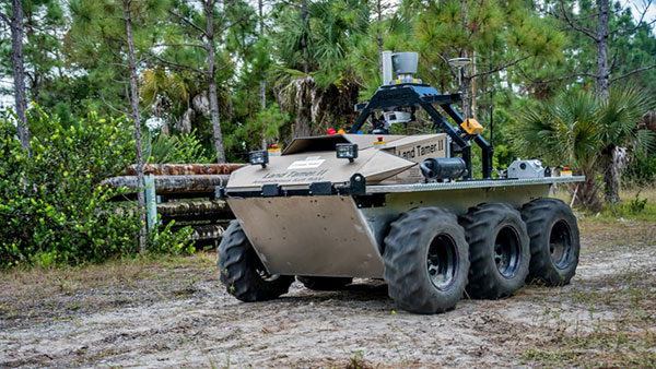
The Black Hawk was equipped for autonomous operation by Sikorsky, a Lockheed Martin Co. It delivered a Land Tamer autonomous unmanned ground vehicle from Carnegie Mellon’s National Robotics Engineering Center (NREC) to a remote site, where the vehicle performed environmental monitoring for potential contamination, the type of robotic mission that could prevent warfighters’ exposure to hazardous conditions, such as chemically or radiologically contaminated areas.
“We were able to demonstrate a new technological capability that combines the strengths of air and ground vehicles,” said Jeremy Searock, NREC technical project manager. “The helicopter provides long-range capability and access to remote areas, while the ground vehicle has long endurance and high-precision sensing.”
The demonstration took place at Sikorsky’s Development Flight Center in West Palm Beach, Florida, for the Army’s Tank Automotive Research, Development and Engineering Center (TARDEC).
Once the helicopter lowered the vehicle to the ground, the Land Tamer drove itself off its transport platform to commence its leg of the mission. The vehicle, equipped with sensors for detecting chemical, biological, radiological or nuclear contamination, then found and surveyed several potentially contaminated sites, autonomously traversing six miles in the process.
When the vehicle sensors detected potential contamination, operators were able to switch the vehicle from autonomous operation into a tele-operated mode for a more detailed exploration of the site.
The helicopter delivered the Land Tamer, Carnegie Mellon’s unmanned ground vehicle. (Photo: CMU)
“The teaming of unmanned aerial vehicles and unmanned ground vehicles, as demonstrated here, has enormous potential to bring the future ground commander an adaptable, modular, responsive and smart capability that can evolve as quickly as needed to meet a constantly changing threat,” said Paul Rogers, TARDEC director.
NREC has developed the unmanned Crusher off-road vehicle for the Defense Advanced Research Projects Agency (DARPA), the Advanced Platform Demonstrator for TARDEC and a tactical unmanned ground vehicle, called Gladiator, for the U.S. Marines, as well as advanced off-road autonomous driving technology. NREC was also part of CMU’s Tartan Racing Team that won the $2 million 2007 DARPA Urban Challenge robot race with its autonomous SUV called Boss.
The Black Hawk helicopter used in the demonstration was a UH-60MU model, equipped for “fly-by-wire” operation. Sikorsky installed its Matrix technology, which it has been developing since 2013.
In the demonstration, a Black Hawk helicopter equipped with Sikorsky’s Matrix autonomy kit flew NREC’s Land Tamer all-terrain vehicle, slung beneath the aircraft in a specially designed cage, to a remote area.
Piksi is a low-cost, high-performance GPS receiver with real-time kinematic (RTK) functionality for centimeter-level relative positioning accuracy.
Its small form factor, fast position-solution update rate, and low-power consumption make Piksi ideal for integration into autonomous vehicles and portable surveying equipment. An open-source architecture with a high-performance DSP on-board and our flexible correlation accelerator make it the perfect platform for GNSS research.
Piksi is designed for autonomous vehicle guidance, such as formation flight and autonomous landing; GPS/GNSS research; and surveying systems.
Swift Navigation is a San Francisco-based startup building centimeter-accurate GPS technology for automotive, surveying, robotics, agriculture and drones.
The company says its products are 100 times more accurate than the GPS in a cell phone, at a tenth of the price of the competition.
In November, the company raised $11 million in a series-A investment round led by Pierre Lamond and Lior Susan at Eclipse Ventures. Swift Navigation plans to use the funds for taking current customers to scale and growing their team, with a focus on core engineering. Another focus continues to be research and development, with a second new product due out this year.
For most GIS professionals, Esri’s new ArcGIS Earth will replace the soon-to-be-discontinued Google Earth Enterprise. I take a tour through the new software, which is much like Google Earth with a few added features. Plus: Q&A from our December UAV webinar.
In early 2015, Google announced that Google Earth Enterprise is being deprecated. In the software world, deprecated means the software is heading towards obsolescence and the vendor isn’t going to develop it further.
Google’s announcement stated that Google Earth Enterprise was being deprecated as of March 20, 2015, but will be supported through March 22, 2017. According to Esri, Google will continue to provide map and location services APIs as well as content.
Here comes Esri, introducing ArcGIS Earth.
At the Esri User Conference last summer, Jack Dangermond announced Esri is working on ArcGIS Earth. Last week, Esri announced the introduction of ArcGIS Earth 1.0. You can download ArcGIS Earth for free.
The opening screen looks a lot like Google Earth, but clearly with an Esri touch via the toolbar in the upper left corner.
You can connect to ArcGIS Online and access its library of data, or import SHP and KML data (no TIF/TFW import, though).
Here are the convenient editing and querying tools (measure).
I imported a KML file containing an orthophoto I created from a UAV flight. Sorry for the orthophoto offset (darned horizontal datum thing).
As it stands now, ArcGIS Earth 1.0 is much like Google Earth with a few added features. However, based on what I perceive Jack Dangermond’s mantra to be, ArcGIS Earth is going to evolve into a powerful mapping tool and platform for consumerizing feature-rich GIS data, much like Google Earth did in the past 10 years, but in a much more GIS way. I look forward to that.
December’s UAV webinar
Speaking of imagery, Google Earth and UAVs, in December I participated in a webinar entitled “Introduction to Using UAVs for Mapping” along with my colleagues from Applanix and C-ASTRAL. If you missed the webinar, you can still view it by signing up here.
It was a solid, 60-minute discussion about the basics of mapping using UAVs. We had a few questions that we didn’t have time to address during the webinar, so I provide answers below. Also, I added some questions that may have been answered, but deserve mention again.
How significant is the quality of GNSS sensors for UAV mapping performance?
In my experience so far, you need precision GNSS measurements either in the air or on the ground if you want high-accuracy results. If you want to use a consumer UAV that has a consumer GNSS receiver in it, you’ll need to use more ground-control points that are mapped with high-precision GNSS receivers. On a wide-open 150-acre site (think agriculture field), that means setting 10-15 ground-control targets. On the other hand, if your UAV has an RTK GNSS receiver in it, you can get by with very few ground-control points. The type of topography also has a significant impact. For example, heavy tree cover, water bodies and other homogenous terrain (such as snow) make it more difficult for image-processing software to process the images.
How accurate can volumes be obtained on stockpiles?
I plan on running some tests and compare volumes computed using terrestrial measurement techniques vs. volumes computed by low-cost UAV images. Based on my experience, I’m willing to wager that the results will be very close.
What are the reasonable accuracies achievable with UAV mapping these days?
With a low-cost UAV (12MP camera), I’m collecting images with a 2-cm/pixel resolution. Horizontal accuracy (with RTK ground control points) is 30 cm or better. Thirty centimeter (30 cm) elevation contours are achievable, and possibly better than that. I’m still exploring how far we can push low-cost UAVs.
Can we use a UAV with our own GPS-RTK base station?
The best use of your GPS-RTK base station is to use it to set RTK ground control for image processing. It’s likely not feasible that you can send corrections from your GPS-RTK base to the UAV unless the UAV is specifically designed to accept those corrections.
Can you tell us the benefits of fixed wing vs. rotary UAVs for mapping work (such as considerations of weather conditions and the benefits of a gimbal-based camera versus a non-gimbal camera typical in fixed-wing UAVs)?
A fixed-wing UAV can cover a much greater area per battery than a rotary UAV, but if you’re located in the U.S., you are restricted to line-of-sight operations. That severely limits the value of a fixed-wing UAV. Fixed-wing UAVs also require a much larger landing area and are trickier to land. It takes much more training to land a fixed-wing UAV than a rotary UAV. I can’t answer your question about gimbal vs. non-gimbal, except that the rotary UAV that I operate has a gimbal for dampening the effects of vibration. With it, vibration doesn’t seem to be an issue.
In forestry, one of the real challenges is stitching the photos together. Did I hear right that RTK will ensure stitching will be greatly improved?
In my limited experience with flying over heavy tree canopy, the best way to handle this scenario is to fly with a heavy overlap (such as 90 percent) or fly at a higher elevation. Since most commercial authorizations in the U.S. limit flight elevation to 200 feet, there’s not a choice to fly higher, so you must fly with a higher overlap.
Eric, could you change the camera to a near infrared camera?
Mine is a consumer UAV, so there’s little support for customization unless I want to really tear it apart myself. There is some after-market support for NDVI and NIR sensors on consumer UAVs, but I’m not knowledgeable about the quality of those. I think that after-market and manufacturer support of various sensors (cameras, NIR, NDVI, lidar) will become more popular on higher-end consumer UAVs.
Eric, the contours seem to capture the curbs in the upper right. Is that correct?
Correct, it’s pretty impressive for a consumer UAV. Granted, I set a dozen or so RTK ground-control points on a 5-acre site, but I’m pretty sure I could cut that in half and achieve the same result. By the way, I should smooth the elevation contours next time.
What software was used to create DEM?
I used Agisoft PhotoScan Pro.
Currently, the use of UAVs seems to be limited to a relatively small project area and required line of sight. Within the natural resource sector, what is the critical barrier at this point to expanding the project size and thus the range of flight — is it technology or air traffic regulations?
In the U.S., the limitation is a regulatory one. The FAA requires visual line-of-sight at all times when operating the UAV. The FAA is testing beyond visual line-of-sight (BVLOS), and we hope that someday BVLOS rules will be issued for commercial operators. For now, you are correct in that UAVs are limited to relatively small areas.
How do the new FAA drone registration rules affect commercial mapping?
According to the FAA, you need to apply for a Section 333 Exemption and CoA (Certificate of Authorization or Waiver) from the FAA to fly UAVs for commercial purposes. This applies even if you want to fly above your own land or even if you don’t charge for flying. If you fly for any other purpose than as a hobby, it gets complicated very quickly.
Look for more content on UAVs in the near future. I’m pushing consumer UAVs to the maximum to see what we can reliably expect from them.
 Epson recently announced in a news release the launch of its Pro G7000-Series large venue projectors for simulators, mapping, digital signage and command centers.