Spirent is one of only 226 organizations in the United Kingdom to be recognized with the Queen’s Award, which acknowledges the company’s excellence in international trade.
Spirent is headquartered in the UK, with its positioning business in Paignton, Devon, developing and manufacturing positioning, navigation and timing (PNT) test solutions. It also has a research and development facility in Daventry, Northamptonshire.
“As reliance on PNT technology continues to grow, our positioning technology business is the trusted partner of the world’s foremost PNT developers, delivering maximum performance without compromise through our dedicated test and validation solutions,” said Martin Foulger, general manager, Spirent Positioning. “We are honored to receive the prestigious Queen’s Award accolade, which is testament to the hard work of our employees in enabling us to achieve such tremendous success worldwide.”
Powered by its international trade, its exports outside of the UK represent a significant proportion of its business, serving a global customer base across five continents and more than 40 countries. Its technology has represented the global gold standard for commercial and government research and development facilities since the inception of GPS.
Its core business is the simulation of GNSS signals in laboratories for the development of applications used in advanced aircraft, chipsets, satellites, smartphones, cars, autonomous systems, marine vessels and defense systems, as well as the navigation systems themselves.
“Market leaders who are developing PNT applications have placed their trust in our test solutions for decades due to our unrivaled performance, realism and reliability,” said Foulger. “Furthermore, Spirent expertise is directly enabling and driving innovation in connected and autonomous vehicles and machine learning, as well as helping to make the world more sustainable through working closely with fields such as smart cities and precision agriculture.”
Now in its 56th year, the Queen’s Award are the most prestigious awards for businesses in the UK and a globally recognized royal seal of approval for companies. As a winner of the award, Spirent is permitted to display the esteemed Queen’s Awards Emblem for the next five years.
Spirent Federal Systems is hosting its annual training seminar in person for the first time in two years. The event will take place July 12-13 in Huntsville, Alabama.
At the seminar, experts in positioning, navigation and timing (PNT) will share the latest GNSS and alternative radiofrequency navigation developments and provide advanced training on Spirent’s test equipment.
The two days of rigorous training includes hands-on workshops and a half-day for official use only (FOUO) session (restricted to U.S. citizens only).
The seminar is free, with breakfast and lunch included. Hotel rooms are additional.
Training topics will include:
Fundamentals of GPS/GNSS Testing
GNSS updates
Basic set-up and use of GNSS simulator
Fundamentals of GPS/GNSS testing
Calibration
Creating Realistic Scenarios
Recreating realistic environments in the lab
Multipath and obscuration modeling
Utilizing remote control and motion
Advanced simulation techniques
GPS/GNSS Vulnerabilities
Interference
Spoofing and other threats
Vulnerability Mitigation
CRPA test systems & anechoic chamber applications
MNSA M-code and Y-code
Alternative PNT navigation
Inertial navigation systems
Flex power
Multi-GNSS constellations
LEO constellation testing
A full agenda will be released soon. The FOUO Session, for U.S. citizens only, will be held on the afternoon of Wednesday, July 13.
Venue. The event will take place 8 a.m. t0 5 p.m. July 12-13 in the Huntsville Marriott at the Space & Rocket Center, 5 Tranquility Base, Huntsville, Alabama.
The Huntsville Marriott is offering a discount for registrants and a limited number of rooms at the government rate. A link to reserve hotel rooms will be provided upon registration.
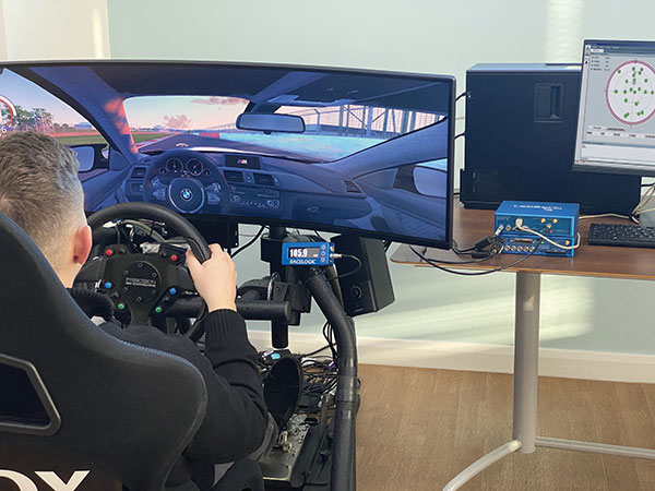
An off-the-shelf PC provides the computing power for complex GNSS driving simulations. (Photo: Racelogic)
By Julian Thomas Managing Director, Racelogic
Driving simulators are commonly used by vehicle manufacturers to expedite the test and development process of their many electronic systems. This not only saves the considerable time and expense of using a real car on a test track, but it is, of course, significantly more environmentally friendly.
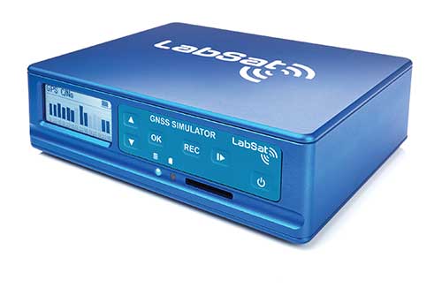
LabSat simulators are used by many leading technology companies and car manufacturers to develop and verify the performance of their new products containing GNSS receivers. These tests are performed using either a pre-recorded or an artificially generated RF signal. This RF signal contains the combination of multiple satellite signals, which are decoded by the GNSS engine, tracking the artificial satellites as though they were real. Static or moving scenarios can be generated, and the user can select parameters to suit their own application, such as time, date and available constellations.
Julian Thomas Managing Director Racelogic
Recently, an automotive LabSat customer had a specific requirement to synchronize a GNSS receiver with the real-time trajectory data generated by one of their driving simulators. This was for a hardware-in-the-loop test rig where a human driver would navigate a route around a virtual test track, while the normal electronic systems reacted as if the vehicle were being driven around a real environment.
The challenge in this customer’s application was that the time delay between the trajectory coming from the simulator and the generation of the corresponding GNSS signals had to be less than 100 ms. This low latency was necessary to achieve realistic synchronization between the driver’s inputs and the resulting output from the GNSS-based device under test.
Traditionally, low-latency real-time simulators use bulky expensive hardware that relies on power-hungry field programmable gate arrays (FPGAs) to create the necessary satellite signals. However, due to the inevitable tick of Moore’s Law, and with some clever optimizations, your entry-level desktop PC now packs more than enough punch to simulate multiple constellations and signals with very low latency.
Using a standard PC to do the heavy lifting means that the hardware required to output the simulated signal is much easier to obtain, can be a lot simpler, and is considerably more cost effective. For example, an 8-core, 3-Ghz Intel i7 processor can generate the signals from 20 satellites in real-time, which normally is sufficient to simulate all but the most complex scenarios.
Our LabSat SatGen software has been continuously developed and optimized during the past 15 years, so it did not take us long to enable the reception of an NMEA trajectory stream with a latency of less than 100 ms. We then streamed this simulated data via USB to our LabSat Real-Time, which generated a corresponding RF signal that can be connected directly to the RF input of any modern GNSS engine.
Using a PC to generate the signals does not mean a loss of fidelity, with the resulting output achieving a repeatable position of less than 10 cm, while the trajectory data can be received at up to 100 Hz.
The resulting solution can take trajectory data from any kind of simulator that has an API to obtain real-time data, such as many popular off-the-shelf driving and flight software simulators, and use this to provide a real-time signal that can be utilized by the GNSS device under test.
Our future development roadmap includes synthesizing external signals, such as CAN-based sensors or inertial measurement units, and then synchronizing these signals with the incoming trajectory. With the amazing power of a modern PC, we are finding that this kind of complex simulation is now much more cost effective and easier to achieve.
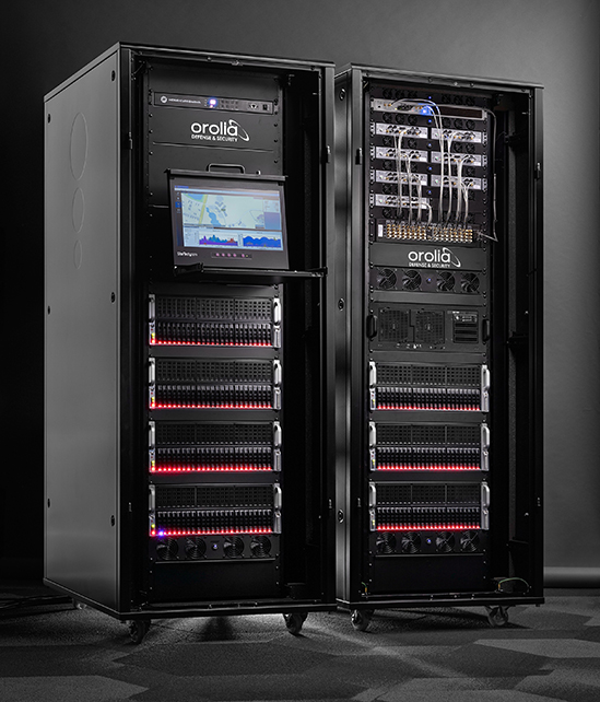
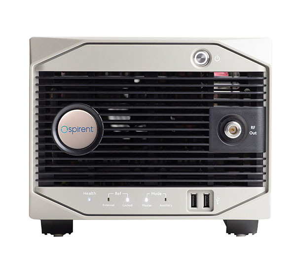
Orolia Defense & Security, provider of software-defined simulation solutions for navigation warfare, will supply a BroadSim Wavefront to the U.S. Air Force Guided Weapons Evaluation Facility (GWEF). BroadSim Wavefront is an innovative, Skydel-powered advanced GNSS simulator.
The BroadSim Wavefront simulator from Orolia Defense & Security. (Photo: Orolia)
The GWEF provides laboratory testing and simulation tools for developing precision-guided weapon technology, including a comprehensive scope of GPS plus inertial navigation systems (INS) and integrated components such as sensors, signals of opportunity and controlled reception pattern antennas (CRPAs). CRPAs are fundamental in many platforms due to their enhanced protection against electronic attacks in NAVWAR environments.
The Broadsim Wavefront simulator will be integrated into a test environment for networked, collaborative and autonomous weapon systems being developed under the Golden Horde program. Golden Horde is one of four Air Force Vanguard programs designed to rapidly advance emerging weapons systems and warfighting concepts through prototype and experimentation.
Of the several capabilities the GWEF required, features such as low-latency hardware-in-the-loop, automated calibration, and the flexibility to quickly integrate future signals and sensors were the most critical and serve as a key reason Orolia’s BroadSim Wavefront was selected. The system will also be capable of testing eight-element CRPA systems, eight simultaneous fixed radiation pattern antenna systems (FRPA), or a combination of CRPA and FRPA systems.
“When designing BroadSim Wavefront, we re-imagined every aspect for the user,” said Tyler Hohman, director of products for Orolia Defense & Security. “Though the GWEF unit contains eight nodes (corresponding to each antenna element), it can be scaled from four to 16 antenna elements. One of the greatest advancements is our continuous phase monitoring and compensation technique. It automatically monitors, aligns and adjusts the phase of each RF output continuously throughout the duration of a scenario.”
“Gone are the days of re-calibrating each frequency on your system, limiting your scenario duration or re-calibration every time you power cycle your system,” Hohman said. “Simply turn the system on, start the scenario, and your Wavefront system phase aligns and remains aligned for the entirety of the test.”
Leveraging the Skydel Simulation Engine, BroadSim Wavefront also supports high-dynamics, MNSA M-code, alternative RF navigation, open-source inertial measurement unit (IMU) plug-ins and a 1000-Hz iteration update rate.
“Because of the software-defined architecture, many upgrades don’t require additional hardware, which has been a crucial advantage for customers who are already using this solution,” Hohman said.
Syntony GNSS has joined TCCA, a global representative body for the critical communications ecosystem.
With offices in France, the United States and Canada, Syntony designs and manufactures GNSS products, including receivers and simulators dedicated to mission-critical applications, transportation, aerospace and defense.
According to an industry report, the global GNSS simulators market size is set to grow from USD 106 million in 2020 to USD 165 million by 2025, at a CAGR of 9.3% during the forecast period. Various factors such as rapid penetration of consumer IoT, the contribution of 5G in enabling ubiquitous connectivity, and increasing use of wearable devices utilizing location information are expected to drive the adoption of the GNSS simulators hardware, software and services.
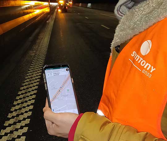
Syntony GNSS manufactures SubWAVE, a solution that enables GPS to work underground and makes possible critical safety services. SubWAVE enables emergency call location in underground tunnels and stations from any smartphone. It also provides the location of any first responder using a compatible P25 or TETRA receiver.
A Syntony team member in a Swedish road tunnel during SubWAVE testing shows the positioning in an underground environment on a smartphone. (Photo: Syntony GNSS)
SubWAVE is typically deployed in underground subway networks (stations and tunnels). It covers 100% of the underground stations of the Stockholm subway, for example. It is also suitable for underground road and rail tunnels, underground parking, and in the mining industry.
“We invented SubWAVE to save lives: to be able to precisely locate a firefighter inside a tunnel, for example, is critical to his or her safety, and this is what our system does,” said Joel Korsakissok, Syntony president and founder. “Also, being able to pinpoint the location of emergency calls made from road or rail tunnels will enhance first responders’ ability to provide assistance and rescue. We are very proud to become a member of TCCA, whose DNA is focused on life-saving through critical communications.”
“Reliable GPS/GNSS coverage in underground and denied locations such as subways, rail and road tunnels and mining is now an essential requirement for emergency services and asset operator personnel navigation and response as well as citizen safety,” said Kevin Graham, TCCA CEO. “General citizens and many businesses now rely on GPS/GNSS signals for their navigation and tracking use cases. We welcome the expertise of Syntony GNSS to enhance knowledge within TCCA of this critical area, and look forward to working with Joel and his team.”
How inertial systems and GNSS availability will help
By Kana Nagai, Matthew Spenko, Ron Henderson and Boris Pervan
Self-driving cars in urban environments can be problematic. The required multi-sensor automated systems will include GNSS, but buildings block and reflect GNSS signals, reducing system availability and accuracy. Researchers from the Illinois Institute of Technology report on how inertial navigation systems coupled with wheel-speed sensors and vehicle dynamic constraints can help.
Innovation Insights with Richard Langley
ARE WE THERE YET? This was a familiar refrain from the backseats of parents’ cars when traveling to a holiday destination or to grandparents when I was growing up. We didn’t have videos on a display attached to the seats in front of us or (who could imagine?) our own personal communication device on which we could call up games, movies or social media channels.
But I’m not talking about that complaint from our childhoods. I’m asking if we have arrived at the era of the self-driving car. The answer is yes and no. It all depends on what you mean by “self-driving.” We reviewed some of the technologies needed for self-driving or autonomous vehicles in this column in June 2019. And we indicated in the introduction to that column that vehicle autonomy has several levels. SAE International, formerly known as the Society of Automotive Engineers, has defined six levels of autonomy that can be briefly described as Level 0 – no automation; Level 1 – hands on/shared control; Level 2 – hands off; Level 3 – eyes off; Level 4 – mind off; and Level 5 – steering wheel optional.
Already, Level 1 automation is widely available in modern cars with adaptive cruise control, parking assistance, lane-keeping assistance and automatic emergency braking among the features being offered.
Level 2 automation, where the automated system takes full control of the vehicle’s acceleration, braking and steering, is available in some production models, although the “hands-off” designation is not to be taken literally — most motor vehicle laws require drivers to keep their hands on the steering wheel.
Between Level 2 and Level 3, we have conditional automation — the car can drive itself, but the driver must stay alert and be prepared to take over immediately.
Level 3 is high automation, where a computer fully drives the car at certain times on certain routes such as a highway; while the driver can perform other tasks such as reading a book, they must be prepared to take over operation of the vehicle within a few seconds if alerted by the automated system. While test campaigns are still ongoing, some jurisdictions permit Level 3 operation by ordinary drivers on some roads, and customers will soon be able to buy vehicles with this level of automation. Widespread use of
Level 4 and Level 5 automation is further off (some would say quite a way off) and remains in development. But famously, last year, Toyota operated Level 4 self-driving shuttle vehicles around the Tokyo 2020 Olympic Village.
A lot more work needs to be done before we will have arrived at the era of the fully self-driving car that will be able to travel on any road, anywhere in the world, all year around, in all weather conditions. In particular, self-driving cars in urban environments (as opposed to highway driving) can be problematic.
The required multi-sensor automated systems will include GNSS, but buildings block and reflect GNSS signals, reducing system availability and accuracy. In “Innovation” this month, researchers from the Illinois Institute of Technology report on how inertial navigation systems coupled with wheel-speed sensors and vehicle dynamic constraints can help.
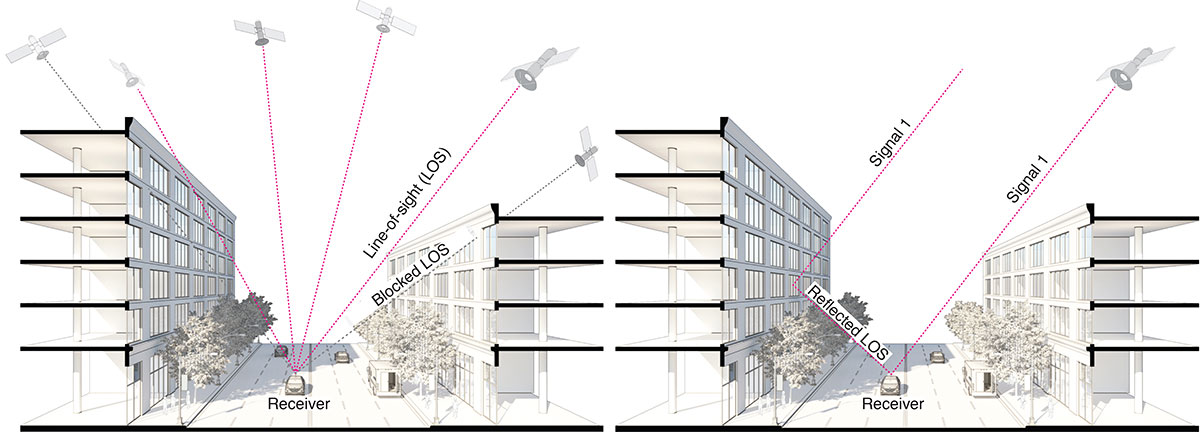
GNSS provides navigation services globally, but satellite visibility in urban areas is limited by high-rise buildings. This creates a mixture of GNSS available and denied environments (see FIGURE 1) — users do not generally know where the system can maintain sufficient levels of accuracy and integrity for a particular application. To begin to address the issue for self-driving cars, we evaluated GNSS-only availability in downtown Chicago.
FIGURE 1. The figure depicts three types of potential GNSS signal reception: direct LOS signals and blocked LOS signals (left) and reflected LOS signals (right). (Image: Authors)
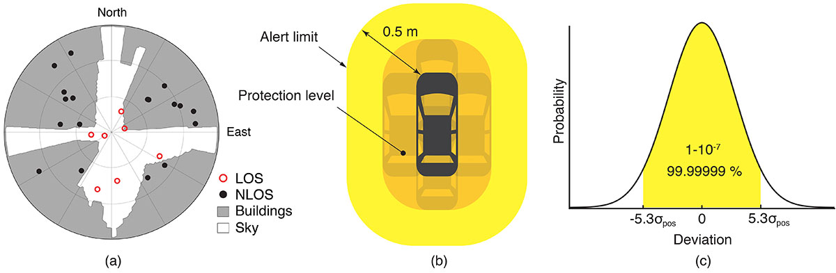
GNSS signal prediction in urban environments has been conducted in previous work. For example, the concept of “shadow matching” was developed to identify GNSS signal blockages in urban canyons. Overlaying sky plots on a hemispherical sky view can be used to distinguish between line-of-sight (LOS) and non-line-of-sight (NLOS) signals (see FIGURE 2a). Reflected rays can be predicted using Householder transformations to reveal potential multipath conditions. Satellites producing blocked or reflected (NLOS) signals should be excluded to maintain integrity.
FIGURE 2. (a) A hemispherical sky view in an urban environment. (b) Illustration of a protection level and an alert limit. To ensure integrity, the protection level must not exceed an alert limit. (c) The allowable probability of exceedance is assumed to be 10−7 in this work. (Image: Authors)
When the number of visible satellites is greater than three, GNSS can resolve vehicle position. However, even in cases where enough satellites are visible, the satellite geometries are generally weak because the dilution of precision (DOP) is adversely affected by the buildings partially blocking the sky. Horizontal positioning error must be bounded by a protection level computed by the vehicle. Then, for navigation to be deemed available, the protection level must not exceed a required alert limit (see FIGURE 2b). The maximum allowed probability of exceedance (see FIGURE 2c) and the alert limit can together be used to determine the maximum allowable position error standard deviation.
Even if the protection level is far below the alert limit in an open-sky environment, it will frequently exceed the alert limit once the vehicle enters a city. GNSS alone is generally not able to maintain availability, so integration with other sensors is needed. Tightly coupling inertial navigation systems (INS) with GNSS using the extended Kalman filter (EKF) provides better estimation in urban environments. The EKF algorithm also enables integration of wheel-speed sensors and vehicle dynamic constraints. These integrated navigation systems will improve availability, but it is still unclear how long such a system can be expected to maintain fault-free integrity in a congested city.
Focusing on the problem of self-driving cars in urban environments, we evaluate protection levels of navigation with practical integrated sensors: GNSS, INS, a wheel-speed sensor (WSS) and vehicle dynamic constraints (VDC). The goal is to develop the means by which we can determine locations where external ranging sources (such as lidar) are needed to maintain continuous navigation with fault-free integrity.
GNSS-ONLY AVAILABILITY
For GNSS availability evaluation, we assume an integrity requirement that the probability of exceeding a 0.5-meter alert limit must be lower than 10−7. The 0.5-meter alert limit therefore corresponds to approximately five times the position standard deviation, so the maximum allowable position error standard deviation is then approximately 0.1 meters. Accuracy at this level clearly requires differential GNSS carrier-phase measurements. We assume a nominal GNSS double difference (DD) carrier ranging error standard deviation of approximately 0.02 meters, and that carrier cycle ambiguities can be readily resolved in an open-sky environment prior to initiation of vehicle motion.
Given the assumptions made of the maximum allowable position error standard deviation and the GNSS ranging error standard deviation, the maximum allowable horizontal dilution of precision (HDOP) is about 5.
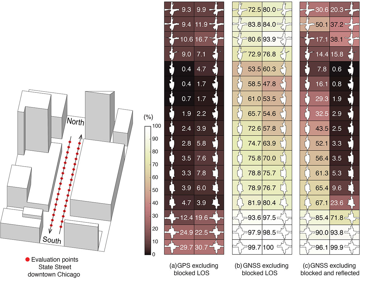
FIGURE 3 shows GPS and GNSS availability — the fraction of time the HDOP requirement is met over 24 hours — along a section of State Street in downtown Chicago. The availability results using GPS only and excluding only blocked LOS signals ranged from 0% to 9% along the block and 9% to 30% at the intersections (see FIGURE 3a). Using four full GNSS constellations (GPS, Galileo, GLONASS and BeiDou), availability ranged from 48% to 82% along the block and 72% to 100% at the intersections (see FIGURE 3b).
FIGURE 3. The percentage of GPS or GNSS availability in 3D-mapped downtown Chicago. We exclude satellites producing blocked LOS signals or both blocked and reflected LOS (NLOS) signals from the measurements. Each column expresses a lane of southbound or northbound travel. The availability is the percentage of total time when HDOP meets the self-driving car integrity requirements in 24 hours. (Image: Authors)
When we also excluded satellites producing reflected LOS signals that reach the vehicle, the availability dropped significantly at every point (see FIGURE 3c). We assert that FIGURE 3c expresses the reality of GNSS availability because building-reflected multipath signals degrade positioning accuracy and would affect integrity negatively. It’s obvious from these results that GNSS alone is insufficient to meet the autonomous driving requirements in an urban environment, and multi-sensor integrated navigation systems are needed to augment poor GNSS signal availability.
MULTI-SENSOR INTEGRATION
We begin by considering tightly coupled INS/GNSS integration using an EKF, and then integrate a realistic sensor suite including WSS and vehicle dynamic constraints that enforce resistance to lateral sliding and vertical movement. If it is known from another source that the vehicle is not moving (for example, it is in the parking gear), a static mode constraint (SMC) can also be applied.
INS/GNSS Integration. Tightly coupled INS/GNSS integration with an EKF uses the INS measurement to predict vehicle motion. The continuous process model uses a state vector having the position in the navigation frame, the velocity, the attitude, bias errors and cycle ambiguities, with the input vector having accelerometer-specific force measurement in the body frame and gyro-rotation-rate measurements. A white-noise vector drives the inertial measurement unit (IMU) states.
The GPS/GNSS measurement model includes the measurement vector having carrier and code phases, and the observation matrix containing LOS vectors and the vector of white receiver thermal noise.
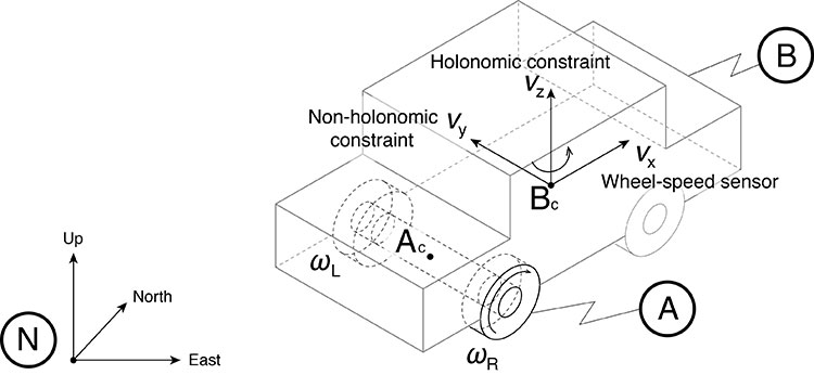
INS/GNSS/WSS/VDC Integration. For the vehicle in motion, we developed a model consisting of a WSS measurement in the along-track direction, a non-holonomic constraint resisting lateral sliding, and a holonomic constraint on vertical movement (see FIGURE 4).
The INS/GNSS/WSS/VDC integration using the EKF consists of the process model and the measurement models.
FIGURE 4. The measurement model consisting of the WSS measurement in the along-track direction (vx), non-holonomic constraint resisting lateral sliding (vy), and holonomic constraint on vertical movement (vz). N is the navigation frame, Ac is the rear-axle center point and Bc is the center point of the body-fixed frame. (Image: Authors)
INS/GNSS/SMC Integration. The static mode constraint provides zero-velocity measurements to the EKF measurement update to mitigate position error propagation. We use SMC only when it is known that the vehicle is not moving; for example, when the vehicle is in the parking gear.
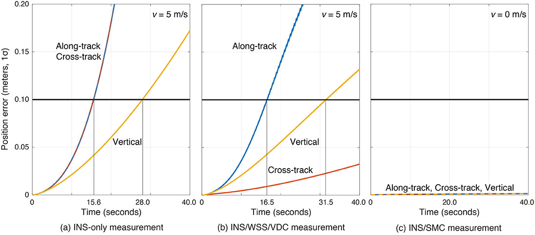
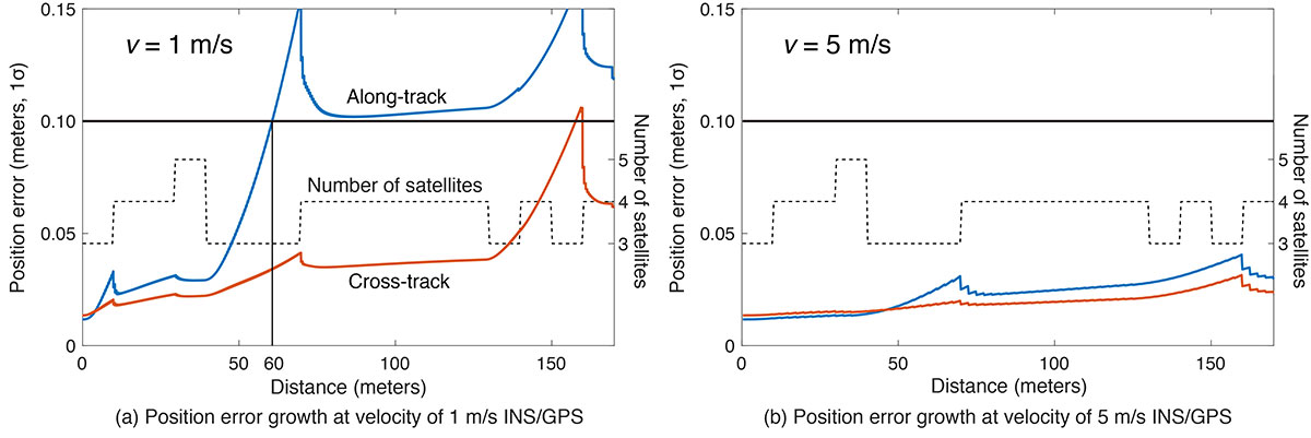
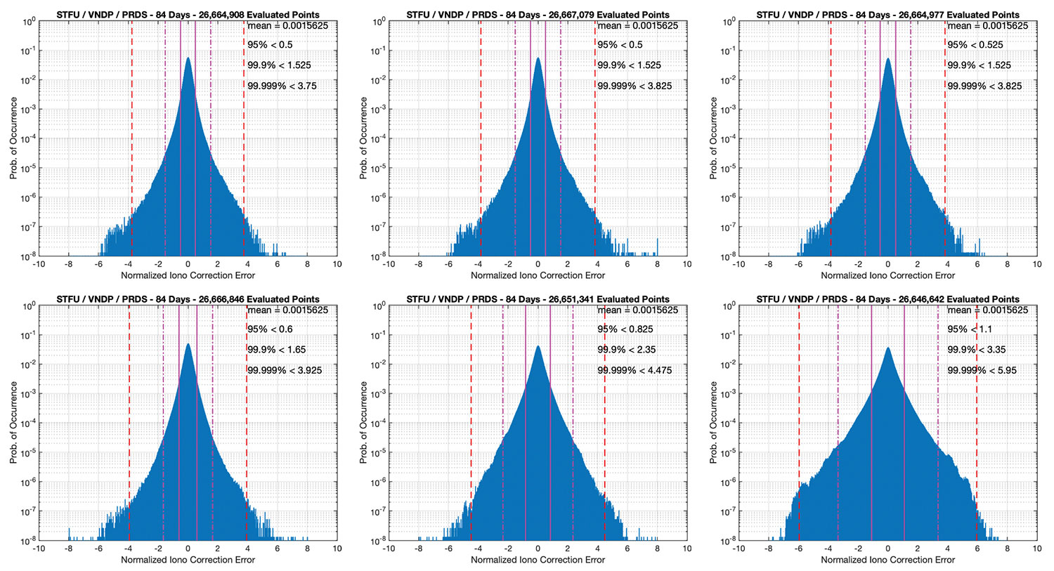
Error Propagation Analysis. We tested the time from perfect initialization to when position error exceeds 0.1 meters in GNSS-denied environments. FIGURE 5 shows the error growth in the along-track (x), the cross-track (y) and the vertical (z). The error specifications for a STIM300 tactical-grade IMU are used in this analysis. The standard deviation of the WSS measurement noise is assumed to be 0.05 meters per second, and the standard deviation of the movement constraint violations is 0.001 meters per second. The vehicle is moving at 5 meters per second except when we test the SMC.
The INS can coast 15.6 seconds before the position error standard deviation exceeds 0.1 meters in both the along-track and the cross-track directions (see FIGURE 5a). The INS/WSS/VDC can coast 16.5 seconds in the along-track direction, and significantly more than 40 seconds (the simulation duration) in the cross-track direction (see FIGURE 5b). In static mode, INS/SMC estimate errors do not grow with time in any direction, as expected (see FIGURE 5c). In GNSS-denied environments, the non-holonomic constraint suppresses the cross-track position error, but the WSS measurement hardly affects the along-track position error. The SMC works perfectly, but the usage is limited to when the vehicle is known to be stationary.
FIGURE 5. The vehicle position error growth vs. time in the along-track (x), cross-track (y) and vertical (z) directions. Each graph represents the navigation system introduced in the multi-sensor integration section. The vehicle is moving at 5 meters per second (a and b) or 0 meters per second (c). (Image: Authors)
SIMULATION SCENARIO
We imagine a future driverless-car mission scenario in which multi-sensor navigation systems are practicable. To minimize congestion in a city, autonomous vehicles will be held outside the urban core when not in use. In the clear open-sky environment, a vehicle in a parking lot completes GNSS initialization using the INS/GNSS/SMC system. Once requested for action, the vehicle departs for the city from the parking lot, and the motion of the vehicle improves alignment by the INS/GNSS system. Safe navigation can be ensured using the system to provide continuity under overpasses and bridges in the open-sky environment. Upon entering the urban core, navigation becomes more dependent on the INS/WSS/VDC system.
A reasonable numerical target for differential GNSS initialized position error is 0.02 meters, and for the INS alignment yaw angle error 0.1 degrees.
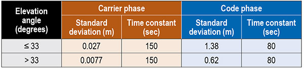
Local GNSS multipath errors from nearby vehicles will vary with the satellite elevation angle. Prior experimental results show that lower elevation-angle satellite signals (below 33 degrees) are much more likely to be impacted by multipath than higher ones (see TABLE 1).
Table 1. The nominal GNSS multipath error values in the simulation.
INITIALIZATION AND ALIGNMENT
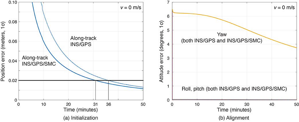
Initialization takes place in a parking lot with a clear sky view. A vehicle is in the parking gear, enabling SMC to be applied. FIGURE 6a shows a typical example: with INS/GPS/SMC, system initialization takes about 31 minutes, and with INS/GPS, about 36 minutes. Therefore, SMC does speed up GPS initialization, although the improvement is modest.
The yaw angle is not aligned during the initialization, but roll and pitch are immediately aligned (see FIGURE 6b). Earth’s gravity affects roll and pitch angle alignment but not yaw angle.
Yaw angle alignment cannot be performed when the vehicle is stationary or moving with constant velocity. Accelerated motion, either straight or turning, is required.
FIGURE 6. (a) Comparisons of initialization time between INS/GPS and INS/GPS/SMC in an open-sky environment. The INS/GPS/SMC system initializes rapidly. (b) Transitions of roll, pitch, yaw alignment during the initialization. Yaw angle alignment cannot be performed when the vehicle is stationary. (Image: Authors)
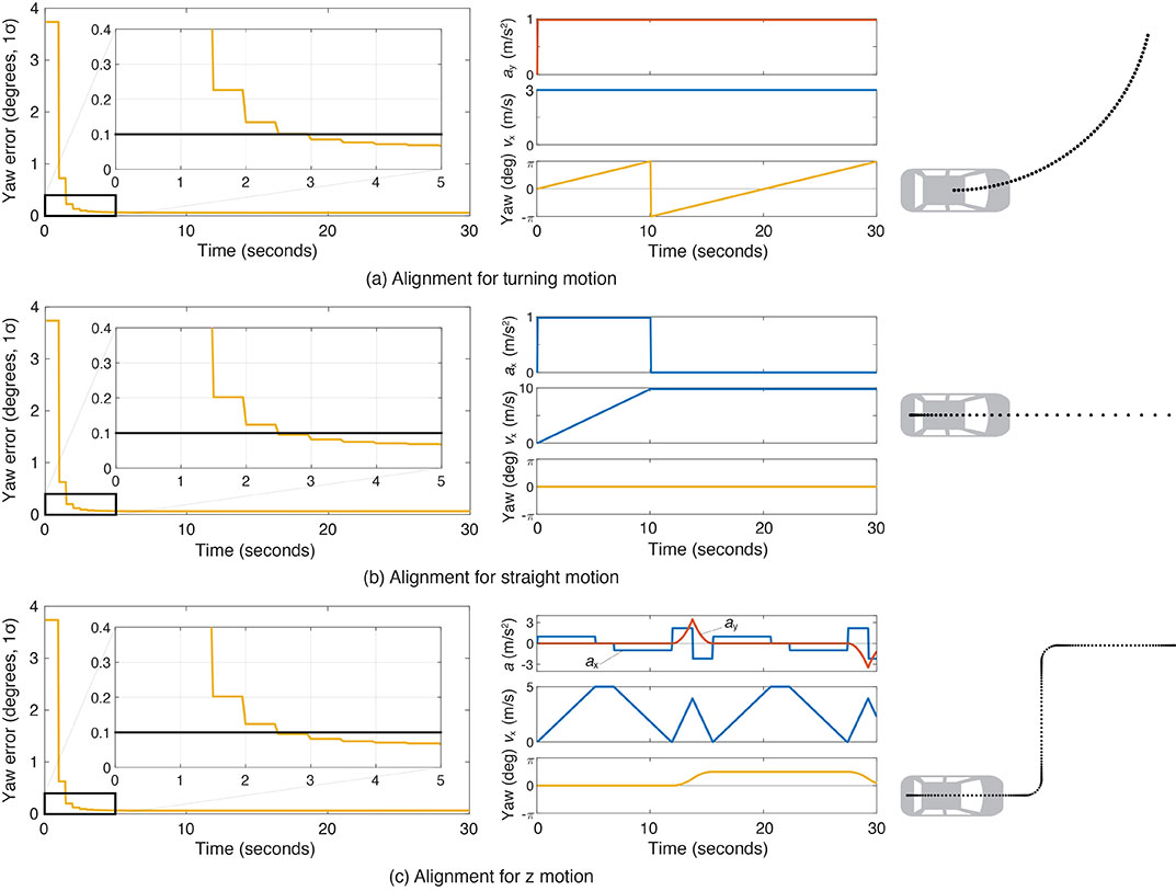
FIGURE 7 shows the behavior of the yaw angle error standard deviation using the INS/GPS system when centripetal (see FIGURE 7a) or tangential (see FIGURE 7b) acceleration is applied. The yaw angle can be aligned in a couple of seconds for either type of acceleration. To represent typical initial motions of self-driving cars, we model a parking-lot departure via a “Z”-shaped path. In this scenario, the yaw alignment error reaches 0.1 degrees within a couple of seconds (see FIGURE 7c).
FIGURE 7. The behavior of yaw angle error when centripetal (a) or tangential (b) acceleration is applied; (c) shows the behavior while following a z-shaped path. The yaw angle can be aligned in a couple of seconds in each case. (Image: Authors)
EVALUATION IN URBAN ENVIRONMENTS
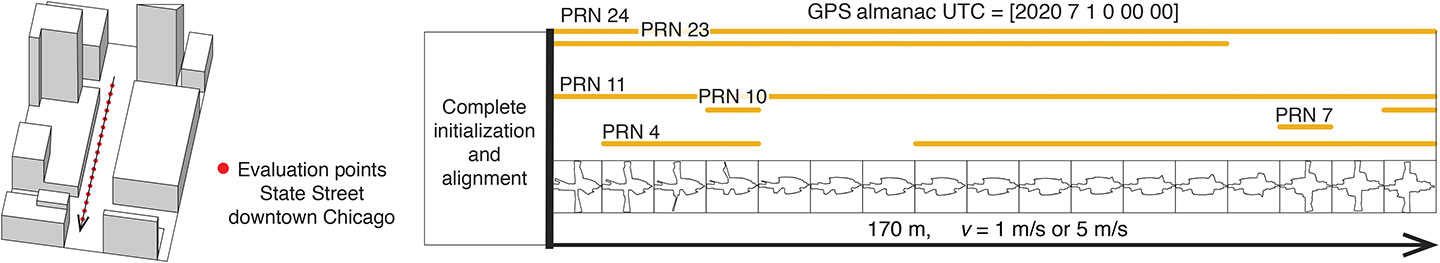
After initialization and alignment in the open-sky environment, we simulated the vehicle traveling into the urban core. The urban environment in our study is 3D-mapped State Street in Chicago, which runs north-south and transits from low-rise neighborhoods to central downtown. We selected one congested section surrounded by tall buildings and computed the position error standard deviation along the path. The evaluation points are at 10-meter intervals over a total distance of 170 meters. The yellow lines in FIGURE 8 denote the visible satellites, identified by their pseudorandom noise (PRN) code numbers, at each point. We assume for convenience that the INS/GPS system is initialized and aligned at the first evaluation point. In reality, we would expect a degraded initial condition because we are starting the simulation in an urban canyon.
FIGURE 8. Evaluation points and PRN numbers of visible satellites at each point. (Image: Authors)
In the first simulation, the car equipped with the INS/GPS system moved either 1 or 5 meters per second. The y-axis in FIGURE 9 represents the position error standard deviation, and the x-axis represents the distance in meters. The dotted line expresses the number of visible satellites. The error when the vehicle velocity is 1 meter per second exceeded the maximum allowable position error standard deviation of 0.1 meter, at the distance of 60 meters. However, when the velocity was 5 meters per second, the maximum allowable position error standard deviation was never reached. It is also clear from the figures that error propagation is significantly affected by the number of visible satellites.
FIGURE 9. A comparison of position error growth between velocities of 1 meter per second and 5 meters per second. (Image: Authors)
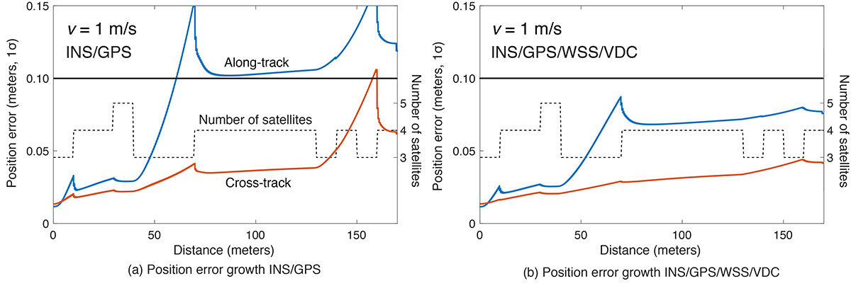
In the second simulation, we compared two different navigation systems, INS/GPS and INS/GPS/WSS/VDC. The vehicle moved at 1 meter per second in the same urban environment. The INS/GPS/WSS/VDC system does provide relief, but the error propagation is still clearly affected by the number of visible satellites (see FIGURE 10).
FIGURE 10. A comparison of position error growth between the INS/GPS and INS/GPS/WSS/VDC systems for a velocity of 1 meter per second. (Image: Authors)
In GNSS-challenged environments, INS error propagation is a function of time. When a vehicle moves faster, it clears the blockage area more quickly, reducing the impact of INS drift — a function of time, not distance. In contrast, GNSS error is completely determined by location. Because INS error propagation depends on how long the vehicle stays in an area of GNSS outage, protection levels for trips through the same area will be different if the vehicle is smoothly cruising or gets stuck in a traffic jam.
CONCLUSION
To gain a better understanding of how long and under what local conditions multi-sensor integrated navigation systems can maintain fault-free integrity, we evaluated navigation positioning errors in 3D-mapped downtown Chicago. The system we developed consists of sensors with which self-driving cars would reasonably be equipped: GNSS, INS, WSS and dynamic constraints. We showed that INS/GPS position errors along the path depend very strongly on the vehicle’s speed. When the system is augmented with WSS/VDC, position errors are suppressed, but the error propagation is still strongly influenced by the number of visible satellites.
ACKNOWLEDGMENTS
The research described in this article is supported by the National Science Foundation. Figure 1 was created by Alexis Arias of the Landscape Architecture + Urbanism Program at the Illinois Institute of Technology (IIT). The authors greatly appreciate the advice and help of Nilay Mistry from that program.
This article is based on the paper “Evaluating INS/GNSS Availability for Self-Driving Cars in Urban Environments” presented at ION ITM 2021, the virtual 2021 International Technical Meeting of The Institute of Navigation, Jan. 25–28, 2021.
KANA NAGAI is a Ph.D. candidate and research assistant in mechanical and aerospace engineering at IIT.
MATTHEW SPENKO is a professor of mechanical and aerospace engineering at IIT. He earned his M.S. and Ph.D. degrees in mechanical engineering from the Massachusetts Institute of Technology.
RON HENDERSON is a professor and director of the Landscape Architecture + Urbanism Program at IIT. He earned his Master of Landscape Architecture and Master of Architecture from the University of Pennsylvania.
BORIS PERVAN is a professor of mechanical and aerospace engineering at IIT. He earned his M.S. from the California Institute of Technology and Ph.D. from Stanford University.
Program will support positioning, navigation and timing (PNT) research at colleges and universities around the world
Orolia has created the Orolia Academic Partnership Program (OAPP) to build a community to help foster global PNT research and collaboration at top engineering schools and research institutions.
Orolia will provide qualified institutions with access to the company’s signature Skydel GNSS simulation engine, an advanced GNSS and PNT testing and simulation tool.
Webinar scheduled
Orolia will host a webinar on Dec. 14 at 11:00 a.m. EST to introduce OAPP and answer questions about the program and Skydel. Register here.
Orolia also created an online forum to support its vision to form an interactive community focused on the future of GNSS and PNT research and education.
The forum allows users to interact with other users and Orolia experts, share information, ask questions and receive feedback. A host of white papers, application notes and detailed technical documents are also available.
The Skydel platform
Skydel is an innovative GNSS simulation platform that leverages software, advanced graphics cards and software-defined radios. Users can build custom signals and connect to other systems and devices (such as sensors and inertial measurement units) through Orolia’s open-source plug-in capabilities.
Skydel also includes the ability to generate and test the vulnerability of GNSS/GPS with integrated interference, jamming and spoofing capabilities. Because Skydel leverages commercial off-the-shelf hardware, it can run independently of simulation vendors’ hardware.
“Skydel platform’s versatility and capabilities allow users to perform tests in the field, in the lab, and at home — whether you are running a turnkey system provided by Orolia, our partners, or through your own proprietary hardware,” said Lisa Perdue, director, PNT Testing and Simulation at Orolia. “Unlike other GNSS simulators, Skydel is the only professional platform offering a plug-in architecture that provides real-time and direct access to the core simulation engine. This plug-in architecture unlocks a new range of application and customization that is impossible to imagine with traditional instruments.”
Perdue added that plug-ins can be shared with the open-source community to leverage all the benefits from a collaborative ecosystem. “We believe this modern architecture is the perfect approach to support academic research as well as allowing users to go further into system integration and customization,” she said.
The University of Stuttgart in Germany is an academic partner. (Photo: Regenscheit, Universität Stuttgart)
Stuttgart Institute a Pioneer
More than 40 schools throughout North America, Europe, South and Central America and Asia-Pacific are enrolled in OAPP, including the Institute of Navigation (INS) at the University of Stuttgart in Germany, where Skydel is fueling pioneering student research.
“Skydel allows our students to carry out complex field tests, such as simulating laboratory scenarios in real time and using radio hardware to send signals to commercial or self-developed receivers,” said Thomas Hobiger, INS. “We can compare our navigation solutions with the simulated trajectories while showing the absolute accuracy of our algorithms, meaning the deviation from the actual position.”
Hobiger added the INS wants graduates to be well-prepared for the demands of the industry and future innovation. According to Statista consumer research, the installed base of GNSS devices worldwide stood at 6.4 billion units in 2019. The Asia-Pacific region led the way, accounting for 3.4 billion GNSS devices, with forecasts suggesting this is set to rise to 5.1 billion devices by 2029.
“OAPP members can contribute to this community to share their advancements, upload code or make their work available to others in our GitHub repository,” Perdue said. “The goal is to ensure that members can access ideas and expertise of other users across the globe.
“The need for continuous and reliable GNSS signals as well as methods to protect those signals from jamming, spoofing or meaconing is growing exponentially worldwide,” Perdue said. “These are the main reasons why engineering students should gain valuable experience using a platform that provides accurate PNT simulation and measurement.”
Hoptroff’s Traceable Time as a Service to become an option for Orolia’s product portfolio; webinar scheduled for Dec. 15
Orolia and timing solutions provider Hoptroff are partnering to deliver a service combining Orolia’s resilient positioning, navigation and timing (PNT) solutions with Hoptroff’s timing synchronization software.
The collaboration will offer Hoptroff’s Traceable Time as a Service (TTaaS) as an add-on to Orolia’s suite of products, providing precise and verifiable time to customers in enterprise, financial, telecom, utilities, public safety, and other markets where traceable time is critical.
Webinar scheduled
Orolia and Hoptroff will host a joint webinar to discuss the partnership and new resiliency options for customers on Dec. 15 at 12 p.m. EST. Register here.
Hoptroff’s TTaaS offers an additional level of security and precision to meet stringent regulatory and resilient infrastructure requirements by delivering accurate time over the network using a VPN connection over broadband or fiber networks.
The bundled solution will simplify the challenge of getting accurate, traceable time in applications where GNSS access is not available or dependable. It can also serve as an accurate, reliable backup to GNSS to provide a high level of resiliency to timing systems being used in critical infrastructure.
“As industries evolve and computer applications become more complex and widely distributed, it is essential that devices in a distributed process share the same accurate timescale to reconstruct digital events after the fact,” said Tim Richards, COO at Hoptroff. “Network-based traceable timing, such as TTaaS, provides resilient backup to a GNSS installation in the case of signal disruption, monitors the quality of performance of time servers, and keeps a record of this timing quality at a location of the customer’s choice. Our partnership with Orolia means businesses will now be able to back up and monitor physical time servers and virtual servers in the cloud, so that they can be sure they share the same accurate timescale, and they have the records to prove it.”
“The partnership with Hoptroff aligns with Orolia’s resilient PNT strategy by providing a wireline solution to augment its space-based PNT solutions. This allows us to further simplify the challenge customers face when building a highly resilient timing solution,” said Jeremy Onyan, Orolia’s director of time sensitive networks. “By combining Orolia’s anti-jamming and anti-spoofing solutions, high-performance GNSS-based timing products, alternative signals like STL, a local high-quality oscillator, and now a wireline-based TTaaS we have one of the most robust portfolios of resilient PNT solutions in the market. Additionally, with the recent acquisition of Seven Solutions, we are well positioned to extend our capabilities into high-accuracy time distribution.”
Seven Solutions is a global innovator in White Rabbit sub-nanosecond time transfer and synchronization technology. “With the capability to distribute time with little to no accuracy loss, Orolia’s customers using Hoptroff’s TTaaS or other time references such as GNSS can extend that time to other parts of their networks and create a high level of resiliency against potential outages,” Onyan added.
By Brandon Weaver, Gianluca Zampieri and Okuary Osechas
Innovation Insights with Richard Langley
IT’S A FACT. GPS and its brethren global (and regional) navigation satellite systems are susceptible to outages caused by both natural and engineered events. Several reports issued in the past couple of decades have documented the vulnerability of GNSS. Twenty years ago this past August, the U.S. Department of Transportation’s John A. Volpe National Transportation Systems Center issued a report, commonly referred to as the Volpe Report, in which they found that “GPS service is susceptible to unintentional disruptions from ionospheric effects, blockage from buildings, and interference from narrow and wideband sources.” Although not explicitly mentioned in the report, besides emissions from communications systems, wideband interference can come from solar radio noise storms overpowering GPS signals. The report also highlighted that the “GPS signal is subject to degradation and loss through attacks by hostile interests. Potential attacks cover the range from jamming and spoofing of GPS signals to disruption of GPS ground stations and satellites.”
The Volpe Report recommended a number of actions to mitigate the vulnerabilities of the GPS signal to disruption or loss, including the need for backups for positioning, navigation and timing — particularly for GPS applications involving the potential for life-threatening situations such as the loss of GPS use for safety-of-life navigation, which would include, for example, aircraft navigation.
With the introduction of GPS (and subsequently the other GNSS and their augmentations) and its widespread adoption by the aviation industry, legacy navigation systems such as Omega, aviation radiobeacons, VHF Omnidirectional Range (VOR) and Distance Measuring Equipment (DME), were either shut down, reduced in their number of installations, or displaced as the primary method of navigation. These systems could not offer the same capabilities as GNSS, and that has led to the high reliance now on GNSS for getting aircraft safely from one airport to another.
But as the Volpe Report pointed out, GPS and (by inference) all other GNSS are susceptible to outages, and so a reliable alternative PNT system that can be readily used for aircraft navigation is needed. Deutsche Flugsicherung, the German air traffic control organization, has proposed such a system, called Mode N. It builds on some aspects of existing navigation systems and aviation-certified signals not originally intended for navigation, including some used for communications and surveillance.
In this month’s column, a team of researchers from the German Aerospace Center introduce us to Mode N, looking at its signal format, required ground infrastructure, aircraft avionics and the potential position accuracy this system could offer.
To accommodate the continued growth of air traffic, air navigation service providers (ANSPs) are planning and implementing programs to increase the capacity and efficiency of airspace. These programs, which include the Next Generation Air Transportation System (NextGen) led by the U.S. Federal Aviation Administration (FAA) and the Single European Sky ATM (Air Traffic Management) Research Programme (SESAR) commissioned by the European Union, heavily rely on GNSS to enable certain capabilities to reach program goals. While intended to serve as the primary source of positioning, navigation and timing (PNT) for aviation services going forward, GNSS is vulnerable to sources of interference. For this reason, efforts have been taken to identify and develop an alternative PNT (APNT) system that can maintain capabilities supported by GNSS when a GNSS outage occurs.
The ANSP for Germany, Deutsche Flugsicherung (DFS), has proposed a concept for such a system that they call Mode N. The proposed design leverages current navigation and surveillance technology to provide a completely new solution to navigation. As the current APNT environment is filled with a variety of proposed solutions spanning the entire field of communications, navigation and surveillance (CNS) technologies, it is useful to describe Mode N within the context of these other APNT systems. This contextual description serves to highlight the interaction of Mode N with current aviation systems — an important consideration for any system intended to serve aviation users. Additionally, as the Mode N design uses similar technological principles as other navigation and surveillance systems, the extensive research performed for APNT can be applied to the Mode N design to provide a preliminary assessment of its navigation performance over Germany.
Development of APNT
The current state of aviation navigation can be simplified by acknowledging that GNSS has replaced legacy navigation systems such as Distance Measuring Equipment (DME) and VHF Omnidirectional Range (VOR) beacons as the primary method of navigation for aircraft. GNSS PNT services enable many capabilities in the airspace that are relied upon by modernization efforts to accommodate the expected increase in air traffic in a safe and efficient manner. Because of GNSS vulnerabilities outlined in the 2001 Volpe Report, it was recognized that an alternative system that could enable the same capabilities as GNSS would be necessary to continue safe and efficient operation of airspace as envisioned if GNSS is unavailable.
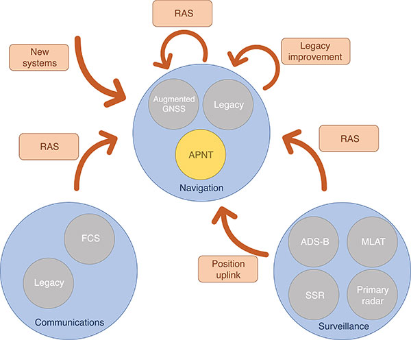
Proposed APNT solutions are generally sourced from the existing CNS environment. A common strategy is to use an aviation-certified signal not originally intended for navigation, which we have termed repurposed aviation signals (RAS). Other proposals include improving legacy systems, transmitting the ground-computed position to an aircraft, and creating new systems entirely. These sources of APNT are summarized in FIGURE 1 with explanations of the abbreviations to follow.
FIGURE 1. Sources of APNT for navigation. (Image: Weaver et al)
A natural candidate for APNT is the use of existing non-GNSS navigation infrastructure. Prior to GNSS, VOR beacons providing beacon-relative heading information and DME navaids supplying two-way range information were the primary navigation infrastructure. Improvement in DME avionics enabled tracking of multiple DME stations, providing a DME-only position solution referred to as DME/DME. Adding DME ground stations and upgrading existing hardware to increase accuracy and coverage of DME/DME positioning was therefore an attractive APNT option.
Another option sourced from the existing navigation infrastructure was to use RAS for positioning. One such RAS is that of the DME reply signal to a non-existent aircraft. By triggering DME responses in a desired fashion, aircraft can use the triggered responses for passive ranging without any change to the DME ground stations.
Communication systems for aviation are also undergoing modernization efforts. Future communication systems (FCS) are being developed to provide broadband communication capability between aircraft and controllers.
Surveillance is the domain of ground-based systems that determine the position of remote objects and is fundamental to allowing safe spacing of aircraft. Its origins reside in the development of primary radar, which was then complemented with secondary surveillance radar (SSR). Both primary radar and SSR use a rotating antenna to measure range and bearing to determine the location of the remote objects. Radar systems tend to be clustered around airports, limiting their area of coverage. To expand coverage in challenging terrain where radar is difficult to install, a technique known as multilateration is used, where a surveillance ground system can receive a signal from an aircraft and determine its position by comparing the time of arrival (TOA) of the signal between its ground stations. These systems were considered as a source of APNT by providing the aircraft position computed on the ground back to the aircraft via data uplink, but timely authentication and integrity concerns have stalled this approach in the United States.
Surveillance RAS for APNT. The other branch of surveillance-sourced APNT is by using RAS, and this is very relevant to the design of Mode N. The system providing many of the RAS for navigation is ADS-B. With this service, an aircraft broadcasts its GNSS-derived position (ADS-B Out) to ground-based stations and any aircraft capable of receiving ADS-B transmissions. ADS-B is an important part of airspace modernization strategies; it is mandated for aircraft operating in most U.S. airspace, with European mandates following suit. ADS-B ground stations, referred to as ground-based transceivers (GBT) or radio stations (ADS-B RS), collect ADS-B Out messages for use by air traffic operators. These ADS-B RS also provide their own transmissions for use by aircraft that can receive ADS-B broadcasts (ADS-B In capability) and include weather information, nearby air traffic and so on.
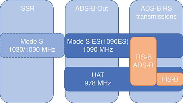
ADS-B can use different protocols to transmit its signals. The Mode S (S for selective) protocol was designed to allow SSR ground stations to selectively interrogate aircraft in their coverage area, reducing congestion on the reply frequency. The Mode S reply format consists of a four-pulse preamble and a data block containing either 56 or 112 information bits for the aircraft to provide information dependent on the interrogation received. Mode S is internationally standardized, and an extended format known as Mode S Extended Squitter was adopted for Automatic Dependent Surveillance Broadcast (ADS-B) services. Mode S Extended Squitter or 1090ES (as it’s transmitted exclusively on 1090 MHz) is also used by the ADS-B RS that rebroadcast ADS-B Out (ADS-R) and provide traffic information services (TIS-B) to nearby aircraft with ADS-B In capability.
Another protocol, used in the United States, is the Universal Access Transceiver (UAT) format. Like 1090ES, UAT is used by certain aircraft to transmit their ADS-B Out messages. Similarly, ADS-B RS transmits TIS-B and ADS-R messages with the UAT protocol; it also includes additional information that it transmits with the Flight Information Service – Broadcast (FIS-B). UAT signals are transmitted in the United States on an unused DME channel frequency of 978 MHz. FIGURE 2 summarizes the relationship between these surveillance signals and the services that use them.
FIGURE 2. Services using Mode S and UAT signal formats.(Image: Weaver et al)
Research investigating the ground-transmitted (ADS-B RS) 1090ES and UAT signals for ranging measurements greatly supports the assessment of Mode N presented here, as the Mode N system operates on a similar basis with a signal that blends characteristics of 1090ES and UAT.
Mode N Overview
Mode N (N for navigation) is a passive ranging system concept from DFS that seeks to provide APNT while reducing the spectrum congestion caused by existing aeronautical navigation and surveillance systems. The design includes the possibility for two-way and air-to-air ranging, but this overview focuses on the preferred passive mode of operation. It is designed around the Mode S format, which as mentioned, is used for SSR and ADS-B services. Despite early references to an SSR/N system, Mode N is not a new SSR mode but rather a new navigation system.
The basic concept is for Mode N ground stations to transmit on a single frequency signals that include ground station ID/coordinates, allowing aircraft with Mode N avionics to receive those signals and determine position in a similar manner to GNSS. As a single frequency is desired to minimize spectrum usage, the ground stations would space their transmissions apart to avoid intersystem interference. This scheme, known as time division multiple access (TDMA), would require information within the signal message on the scheduled time a ground station transmits, which the Mode N format allows.
Because Mode N shares many design aspects with Mode S, DME and other surveillance RAS, it is able to leverage previous APNT work for the benefit of its own analysis. Therefore, the overview of the design is described here relative to other APNT systems, as this is the basis of the preliminary performance assessment we present.
The Mode N Signal. The Mode N design proposes using the Mode S downlink signal format as the basis for its ranging signal to be used by the aircraft for passive position determination, with some key differences. The frequency channel on 1090 MHz is too congested to accommodate more signals; thus, the first difference is that Mode N intends to transmit on a different frequency. While the channel selection is still ongoing, unused DME channels have been identified as options for frequency allocation.
The second difference is the message content. As the Mode S downlink format transmits mainly aircraft-specific information, Mode N ground transmitters would instead populate their messages with information needed for passive ranging: ground station coordinates and time of transmission (TOT). The study of 1090ES messages (which also contain aircraft-specific information despite being transmitted by ground stations) as RAS required some special techniques to first identify which station was transmitting the message. The TOT is not present in 1090ES signals, but more importantly the time of transmission is not synchronized to any consistent reference. Aside from transmission frequency and message content, the Mode N signal design follows the Mode S downlink format (modulation, pulse shape and so on).
The Mode N signal also shares some aspects with the UAT signal, particularly the FIS-B segment. First, UAT is also transmitted in the United States on an unused DME channel. The FIS-B message, which provides weather information, transmits the ground station coordinates and information that can be used to estimate the TOT. Specifically, UAT messages are synced to UTC, and each ADS-B RS has a designated time slot within a one-second interval where it transmits its FIS-B message. This time slot is included in the message, and can be used to determine the TOT of the signal. Mode N is designed to work in this exact manner, minus the weather information. One crucial difference between UAT and the Mode N design is the type of modulation. Like Mode S, Mode N proposes using pulse-position-modulation (PPM) or on-off keying (OOK). The resulting wider bandwidth — estimated to be less than 4.6 MHz at –3dB — has better resistance to multipath, whereas UAT is frequency modulated to maintain a narrow bandwidth to avoid interference with DME and is more susceptible to multipath. Research on UAT signals for pseudoranging capability (also determined at a higher update rate than once per second) would be necessary for navigation, an important consideration for the final Mode N design.
Ground Infrastructure. The Mode N design, while based on RAS from the surveillance capability, requires new ground stations to transmit the Mode N signal. Requirements for the ground stations are that they provide adequate coverage to meet the requirements of an APNT system and that they are sufficiently synchronized in time. An initial time-synchronization scheme is the use of a radio frequency (RF) network consisting of the ground stations themselves, which requires radio line-of-sight of stations throughout the network. DFS performed a study and found that additional time-beacon stations would be necessary to maintain this RF time network, even though navigation coverage was provided using existing DME sites as hypothetical Mode N stations. Since these aspects of the design are still developing, the preliminary assessment we present assumes a network layout and time synchronization tolerance. As the Mode N design blends various CNS principles, a natural baseline design for the ground station locations consists of existing DME and surveillance sites in Germany. Using these locations for the ground stations enables computation of a horizontal dilution of precision (HDOP) at discrete locations throughout Germany. The assumed time synchronization is discussed further when developing a model of the Mode N ranging accuracy.
Avionics. An interesting aspect of the Mode N design is its proposed avionics unit. The Mode N avionics must be capable of receiving Mode N messages, which it can do with the existing DME antennas on aircraft. The Mode N avionics unit must then decode the messages for position determination. Its active mode for two-way and air-to-air ranging would require the Mode N avionics to transmit Mode N messages, again using the existing DME antenna.
Recognizing the continuing investment in the DME network by multiple countries, the Mode N avionics sensor is essentially built around a fully functional DME unit. This is intended to provide a seamless transition as Mode N stations are brought on line. The design of the avionics has little effect on the coverage assessment, aside from guaranteeing a minimum level of performance based on the current DME network, but is an important part of the implementation strategy. Furthermore, this blend of avionics has also been proposed for a unit compatible with DME and ADS-B (1090ES and UAT) signals.
Preliminary Coverage Assessment
Preliminary coverage assessments are a typical method to determine the feasibility of a proposed system to provide the required level of performance over a given area. A simple method of characterizing the position performance is in terms of the linear relationship between range error and DOP, where the range errors are assumed to be zero-mean, uncorrelated, and have identical distributions.
As the aircraft is assumed to have additional sensors for determining its altitude, HDOP is commonly used to characterize the expected horizontal position performance.
With range measurements, HDOP is a function of the transmitter geometry available to an aircraft at a given point. It is a straightforward computation to perform for a grid of points over the area of interest. The HDOP computation does depend on the type of range measurement, so passive (pseudo-) range, two-way range, and time difference of arrival (TDOA) measurements all have their corresponding DOP computation. Determining a model for the range error is less straightforward, and assessing the coverage potential of Mode N requires an estimation of the expected range error.
Modeling Mode N Range Accuracy. As Mode N is not an existing system, abundant quantities of real measurements are unavailable for empirically characterizing the range performance. However, since Mode N is heavily based on the Mode S signal format and functions similarly to the DME and UAT signals, which all exist and have been measured extensively, research investigating those signals can help derive the model for the Mode N range performance.
An alternate approach is to reference the standards for a specified performance level. For example, ICAO documentation specifies that the Airborne Collision Avoidance System (ACAS) logic use a zero-mean normal distribution range error model with a standard deviation of 50 feet, or about 15 meters. As ACAS also uses the Mode S signal format, this appears to be a reasonable source for the Mode N range error. However, since ACAS is an airborne two-way surveillance method, it does not exactly translate to a ground-based passive TDOA system such as Mode N. The 15-meter standard deviation is still useful, as it provides a check on the estimated Mode N accuracy. Other specifications suffer from similar drawbacks — Mode N does not directly apply to any single system. Thus, we apply the blended approach using previous APNT research.
The fundamental measurement for the passive ranging mode of Mode N is the TDOA between pairs of ground stations. This measurement is in seconds, and is translated to a range difference by using the speed of radio signal propagation in a vacuum. (See our conference paper for further details.)
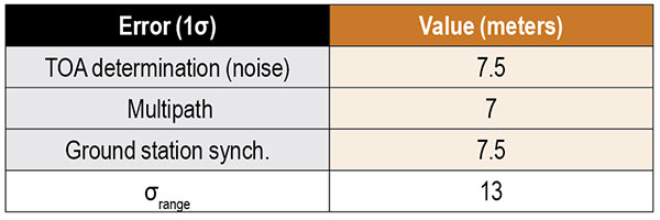
Errors can be present in the TOA measurement, synchronization of the nominal TOT of the signals, and parsing of the time slot data field. The TOA measurement can have errors by inaccurate determination of the actual TOA due to noise or multipath and by the actual TOA differing from the nominal arrival time of the signal due to atmospheric delay. For terrestrial systems, propagation errors are considered to be dominated by multipath, so we don’t consider atmospheric effects here. Time synchronization errors are very important to the ranging accuracy, but it is assumed the time slot data field is parsed accurately. Other sources of error, such as inaccurate ground station coordinates, can affect the position error but have no effect on the range error. Additionally, the error originating from the change in aircraft position between reception of signals at ground stations is not considered in this article. The model of range accuracy can then be expressed as the root-sum-square (RSS) of the dominant individual error components.
We studied each error component in isolation, selecting the applicable APNT research to leverage based on the Mode N design aspect that most corresponds with that error.
Since the Mode N design also uses a pulsed signal, the evaluation of DME (specifically, DME/N) ranging performance is the starting point for estimating the TOA noise error. Part of the APNT effort was evaluating current DME performance, as it was thought it exceeded the specified performance in standards. A study found that current DME performance allowed a budgeted TOA error of 15 meters, 2σ.
For the Mode N error model, a 7.5-meter error is an attractive option to choose as it is the average of two other sources and is the most recent. This value is a conservative estimate of the TOA accuracy for Mode N because the Mode N/S pulse shape is narrower than the DME pulse with a greater bandwidth, improving theoretical accuracy. For the preliminary coverage assessment, a conservative estimate is desired, because the actual TOA accuracy will vary over an area depending on transmitter distance — which impacts the level of signal noise. Note that the DME TOA errors are not divided by two as is done for the total DME error as they apply to a one-way TOA measurement.
After assessing the relevant studies, we modeled the multipath component of the error following that from Mode S as 7 meters, 1σ.
The final error component to estimate for Mode N is that of the synchronization of the ground stations. Based on the results from studies of the UAT signal and those from eLoran, we set a 15-meter maximum bias as a 2σ error component in the Mode N error model.
Our error analysis is summarized in TABLE 1.
TABLE 1. Predicted Mode N range accuracy. (Data: Weaver et al)
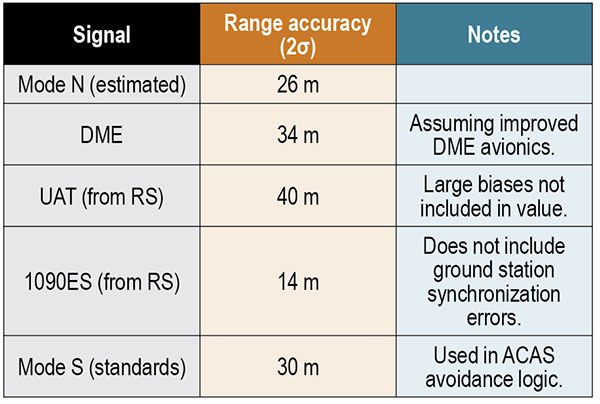
A total 2σ error for current DME performance of 92 meters has been established, which translates to 46 meters of range accuracy after dividing by two (since the DME signal is a two-way range). A substantial part of this error derives from the avionics bias, which is minimized for a “potential” DME error budget due to an assumed improved avionics performance. This results in a DME range 2σ error of 34 meters. We chose this value to compare as the effect of avionics has less of an impact in a passive ranging system such as Mode N.
Range performance for UAT signals was evaluated with measurements showing 20-meter (1σ) error when compared to GNSS truth, not including large biases attributed to ground station synchronization or processing errors. The 1090ES signals do not have an inherent ranging capability, so the TDOA measurement error of two ground station signals to one receiving station is difficult to measure. Instead, researchers have measured the differential TOA (DTOA) of one ground station signal received by two (GPS-synchronized) receiving stations to first identify which station transmitted the signal. When compared to the true DTOA based on ground station and receiving station coordinates, the measurements contained small biases around 10 meters with a standard deviation also less than 10 meters. Being DTOA measurements, these do not contain ground station synchronization errors, so the reported standard deviations correspond mostly with propagation and determining TOA. The 10-meter DTOA 1σ error can still be converted to a range error resulting in 14 meters (2σ). These results are summarized in TABLE 2.
TABLE 2. Comparison of Mode N with other APNT signals. (Data: Weaver et al)
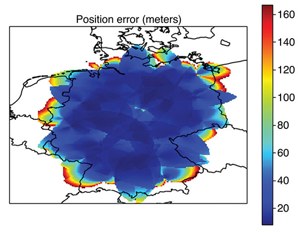
Coverage Assessment. With the estimated ranging accuracy, a preliminary coverage over Germany could now be assessed. Using the current 29 surveillance site locations in Germany and assuming that a minimum of three stations is necessary for positioning, the estimated position accuracy is shown in FIGURE 3.
FIGURE 3. Estimated position error (in meters) for aircraft within a 100 nautical mile coverage radius using existing surveillance sites as installation locations for Mode N ground stations. (Image: Weaver et al)
The coverage assessment used a “flat” Germany model with the estimated range accuracy from the preceding section (13 meters, 1σ). Atmospheric and terrain considerations were not applied in the assessment. It is important to note that this level of coverage would degrade at lower altitudes.
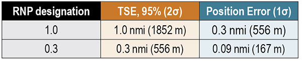
To determine whether this level of accuracy is sufficient for the airspace modernization efforts in Europe, the desired Required Navigation Performance (RNP) accuracy requirement must be examined. For RNP 1.0, where 1.0 refers to the required 95% or 2σ total system error (TSE) accuracy in nautical miles, the position error allocation is assumed to be 30% of the RNP/TSE value. The required position accuracy is shown in TABLE 3.
TABLE 3. RNP required horizontal position accuracy. (Data: Weaver et al)
From Figure 3, aircraft at altitudes within the service volume supported by a 100-nautical-mile coverage radius are capable of meeting the accuracy requirement for RNP 1.0 and 0.3 within most of Germany. Coverage along the border is unavailable as only German surveillance site locations were used.
Conclusions
Although our derivation of accuracy and the coverage assessment method we used made several simplifying assumptions, the results indicate that Mode N has the potential to be a feasible APNT system. To be a part of the modern airspace navigation infrastructure, additional accuracy requirements must also be met. The integrity requirement is harder to meet than accuracy, and requires either redundant information available to the aircraft for a receiver autonomous integrity monitoring-like algorithm or a ground-based monitoring/augmentation system. Perhaps the biggest challenge to implementing the Mode N infrastructure is maintaining an RF-based time synchronization network. Convincing aircraft operators to update their avionics is another challenge to Mode N implementation, although the inclusion of DME functionality in the Mode N avionics seeks to ease that transition.
DISCLAIMER
The views expressed herein are those of the authors and are not to be construed as official or reflecting the views of Deutsche Flugsicherung.
ACKNOWLEDGMENT
This article is based on the paper “An Overview of the Proposed Mode N System in the Context of Alternative Position, Navigation, and Timing (APNT) Development” presented at ION ITM 2021, the virtual 2021 International Technical Meeting of The Institute of Navigation, Jan. 25–28, 2021.
BRANDON WEAVER is a researcher at the German Aerospace Center (DLR) and works on alternative navigation systems.
GIANLUCA ZAMPIERI joined the Alternative Navigation Systems Group at DLR’s Institute for Communication and Navigation in 2019.
OKUARY OSECHAS leads the Alternative Navigation Systems Group in the Institute of Communications and Navigation at DLR.
The General Lighthouse Authorities (GLA) of the United Kingdom and Ireland has named Alan Grant to the top post of its research and development team. Grant assumed his new role on Nov. 1.
As part of his duties, he heads the GLA’s research and development program, considering existing and future maritime requirements and operational strategy. GLA Research and Development (GRAD) is tasked with improving maritime safety by developing innovative and cost-effective maritime aids-to-navigation (AtoN).
GRAD projects have included all aspects of AtoN including human and machine interaction, operational life and environment. The team has deep technical expertise and experience with automatic identification systems (AIS) , the VHF Data Exchange System (VDES) , eLoran, e‑navigation, GNSS, SBAS and visual signaling.
The organization is well known for its expertise in electronic navigation aids and was an important contributor to the MarRINav project. The project effort was funded by the European Space Agency and examined what combination of electronic aids to navigation are needed to ensure uninterrupted UK shipping.
Grant joined the GLA in 2003 and has worked on a variety of systems during his time with GRAD. He led a series of successful GPS jamming trials and the development of the multi-system radionavigation receiver performance standards, from initial concept to international recognition at the IMO. He continues to support resilient positioning, navigation and timing in maritime navigation at both technical and strategic levels.
Grant is a Fellow of the Royal Institute of Navigation, where he is a member of the council and served as vice president, 2019-2021. He is also a member of the U.S. Institute of Navigation and served on the ION Council, 2013-2017.
Grant chairs the International Association of Marine Aids to Navigation and Lighthouse Authorities (IALA) radionavigation services working group and is a member of several international standards bodies. He is a chartered engineer, a chartered physicist, and author of more than 120 journal papers, magazine articles, and conference papers.
Martin Bransby, the prior GRAD leader, has taken a position with Telespazio in the UK.
Longstone Lighthouse is situated on the Outer Farne Islands on the Northumberland Coast in Northern England. (Photo: ad_foto/iStock/Getty Images Plus/Getty Images)
Simulator vendors explain their evolution in response to changes in GNSS/PNT, comment on technical challenges they face, and outline principal markets.
GNSS receivers — which were never as simple as FM radio receivers or garage door remote controls — are becoming increasingly complex. The causes for this include continuing efforts to:
reduce their size, weight, and power (SWAP)
utilize new signals from up to four GNSS constellations
integrate them with other sensors, such as inertial measurement units (IMUs), cameras, and lidars
take advantage of a growing number of public and private, global, regional, and local correction services
meet the requirements of booming new markets, such as autonomous vehicles
mitigate the threats posed by the proliferation of unintentional and intentional RF interference, the latter better known as jamming, and by spoofing.
In short, receiver manufacturers must constantly adapt to a GNSS/PNT landscape that is, as one of the respondents to this Q&A put it, “ever evolving.”
In turn, the growing complexity of GNSS receivers requires increasingly sophisticated simulators to test receivers and their integrations in controlled conditions before field testing and deployment. Increasingly, this is achieved by replacing with software what was once done in hardware. Simulation remains a vital, though often underappreciated, segment of our industry.
On the following pages, five simulator vendors briefly explain their evolution in response to changes in GNSS/PNT, comment on the principal technical challenges they face, and outline their principal markets.
Spirent Federal Systems’ GSS6450 RF record and playback GNSS simulator is portable, for testing automotive applications in the field. (Photo: Spirent Federal)Lisa Perdue Product Line Director, Simulation Orolia
OROLIA
How has your approach to simulation changed over the years and in response to what changes in GNSS/PNT?
We have transitioned away from the GNSS simulator approach of using fixed, allocated hardware that we used in our early simulators to the more modern software-defined approach we use today. Given the ever-evolving PNT landscape, it is difficult to design hardware that will support all future GNSS and PNT simulation needs. Instead, we focus on the development of the Skydel software platform, which can then be used with the supported COTS hardware or turnkey system to generate the necessary signals. This gives us the benefit of maximum scalability and flexibility while being truly future proof.
The software-defined approach also allows us to offer Skydel in new and exciting ways. We aim to make PNT simulation accessible to everyone and we can do that through subscription and cloud-based simulation services.
What are currently the greatest technical challenges to GNSS/PNT simulation?
Today GNSS is only a part of the PNT picture. GNSS receivers are often tightly integrated with other sensors and many times the GNSS receiver cannot be isolated to test it on its own. Other sensors must also be stimulated or simulated and included as part of testing. Correction services are becoming more common, but many are proprietary with no public specification. With no common standards available, it can be technically challenging to create a one-size-fits-all test solution.
We tackle these challenges through our plug-in feature. The plug-in architecture allows you to expand the capabilities of Skydel by adding your own features or complex integration with other systems. It allows you to exchange information with the Skydel Engine and even integrates it into the Skydel UI. With our open-source SDK, which includes example plug-ins, you can create your data outputs synchronized to the GNSS simulation, such as IMU or correction services data.
In what markets and applications are your simulators used? Are they used only in labs or also in the field?
At Orolia, we say ‘Skydel Everywhere.’ Skydel is used in applications ranging from military encrypted receiver testing (SAASM, M-Code, PRS) to commercial applications supporting any of the GNSS signals available.
Skydel is used in systems that are found in labs, but you can also find Skydel at an individual engineer’s desk, or even home offices. In the field, Skydel has provided simulation and threat generation capability to authorized test ranges and field test events.
The broadsim software-defined GNSS is powered by Orolia’s Skydel GNSS simulator engine. (Photo: Orolia)
RACELOGIC
Julian Thomas Managing Director Racelogic
How has your approach to simulation changed over the years and in response to what changes in GNSS/PNT?
Over the years, GNSS technology has changed significantly but our approach of identifying a need and creating a solution hasn’t changed since we launched our first LabSat GNSS simulator. We created LabSat because we needed a cost-effective, accurate and easy to use record and replay simulator that we could use for product development and production line testing for our VBOX Automotive and VBOX Motorsport technologies. This need could not be met by any other simulator manufacturer, so we developed our own solution, which in turn became LabSat. Although our approach has not changed, the needs of users, including our own engineers, have, so we continue to develop and improve LabSat to meet these needs.
With the increasing number of satellite launches in market segments such as communication and navigation, the number of requests for testing space-qualified receivers has increased dramatically. To test these kinds of scenarios, we have been making some major upgrades to simulate rocket launches and Earth orbit trajectories that require very different characteristics from land-based simulation.
As the number of constellations and signals has expanded very rapidly, the number of simultaneous signals that need to be simulated has put a far greater requirement on the computing power needed to render them. We have been working very hard on optimizing our routines to make the most of the new breed of high-performance multi-core processors. The result has been a big decrease in the time taken to create a scenario, and an increase in the number of signals that can be simulated in real-time.
What are currently the greatest technical challenges to GNSS/PNT simulation?
The biggest challenge is in simulating a large number of constellations and signals in real-time without using dedicated, expensive hardware to create them. The good news is that with the latest Intel Xeon processors boasting up to 40 cores and 80 threads, a much larger number of signals can now be created in real-time using off-the-shelf PC components.
In what markets and applications are your simulators used? Are they used only in labs or also in the field?
With the global pandemic causing national lockdowns, many engineers switched to working from home. Our largest growth in the simulator market has therefore been due to providing these engineers with a small, low cost, easy to use simulator that they can have on their desks at home, allowing them to continue to develop GNSS applications without having to go into the office. The markets these engineers work within are as varied as the markets that use GNSS technology.
We have also seen a big increase in the use of our simulators to test mass produced satellites used in providing global internet coverage. These satellites are being produced in large volumes, and the need for a low cost, reliable testing method on the production line has driven strong growth in this area.
Our simulators are often used in the field to gather data for in-lab testing, as small size and battery life are very important factors in this environment.
SPIRENT FEDERAL SYSTEMS
Phillip Bonilla Senior Systems Engineer
How has your approach to simulation changed over the years and in response to what changes in GNSS/PNT?
Spirent has provided highly accurate simulation solutions since the early phases of GPS availability, starting with defined hardware for each signal type. As the GNSS landscape has grown, Spirent has worked closely with leading developers, adding key flexibility and functionality to adapt and provide a growing product portfolio. By adopting a robustly defined system architecture, and employing signal-agnostic hardware, Spirent simulators can generate any of the available constellations and frequencies, with no more than a few clicks of a mouse.
While broadening the support for the increasing number of constellations has been a focus, so too has the necessity to provide users with high numbers of available channels and auxiliary simulation needs. To complement GNSS simulation, significant effort is being devoted to resilient application testing, providing users with flexible solutions for introducing jamming and spoofing to the test environment. Our agnostic hardware supports signal generation using software defined radio (SDR), including interference sources and user-defined IQ signal data. As customer demands have grown, alternative RF and PNT sensors have been—and continue to be—incorporated, allowing users an expanded and comprehensive test environment.
The new spirent simulator generates alternative RF navigation signals concurrently with GNSS signals. (Photo: Spirent Federal)
What are currently the greatest technical challenges to GNSS/PNT simulation?
Today, nearly all industries rely on GNSS or other PNT sources to some extent. With such varied and widespread use, laboratory testing is critical, and maintaining the highest levels of accuracy, reliability and robustness remains one of the greatest challenges. For modern hardware-in-the-loop configurations, simulation systems must be able to keep latency consistent to enable powerful post-processing of results. With this challenge in mind, we at Spirent design and manufacture our own hardware, ensuring precision and ultra-low latency.
Another significant test challenge posed by modern applications is the growth in vehicle speed and maneuverability. Creating a truly realistic test environment for supersonic and even hypersonic vehicles with high rates of spin and jerk places huge demands on a simulator. Spirent recently has introduced the industry’s first 2 kHz update rate, enabling the most accurate trajectories for the most mobile technologies.
Lastly, positioning engines are becoming more complex. In addition to GNSS and inertial, vision systems and a range of other sensors and signals-of-opportunity are providing developers greater opportunity for precision and robustness. Therefore, a core part of Spirent’s mission statement is delivering test equipment that is designed to be integrated into wider test benches and ensuring that equipment is always orders of magnitude more accurate than any device under test.
In what markets and applications are your simulators used? Are they used only in labs or also in the field?
Spirent simulators are used in all phases of the product life cycle across nearly all applications. Receiver manufacturers use our solutions beginning with initial research and development, throughout product development, and well into production and field testing. Along with the ability to use Spirent’s simulators for live range testing, Spirent’s GSS6450 record and playback system enables users to record the real world in high dynamic detail for repeatable lab testing.
JACKSON LABS
Gregor Said Jackson President and CTO
How has your approach to simulation changed over the years and in response to what changes in GNSS/PNT?
Initially, we saw a large demand for GPS-only solutions. We are shipping units into this market and it is growing more than 30% year over year for us. Recently, customers are looking to also supporting other constellations. There is an emerging market for LEO simulation capability. Many LEO constellations are becoming reality, such as OneWeb, Kuiper, Starlink, Iridium, Xona, and others, and customers are more frequently asking if we can support these types of signals in our simulators. Demand also is arising for additional base-band signals to accommodate the RF signals, such as synchronized raw IMU data and other observables. Jamming and spoofing signals also are being requested and reproducing these as faithfully as possible is a big challenge for synthesized simulation. Lastly, we see demand rising for mil-type secure applications, such as M-Code, PRS (Galileo) and P(Y) code SAASM of course. The complexity of future simulators will rise in lockstep with the complexity of the RF spectrum coming to us from space.
What are currently the greatest technical challenges to GNSS/PNT simulation?
The STL-1400 positioning and timing receiver is designed for battery-operated low SWaP-C applications. (Photo: Jackson Labs)
A faithful reproduction of the real live-sky RF signals would rank high on this list. There are almost an unlimited number of out-of-band and in-band benign and adversary RF signals on a typical GNSS antenna these days, and more recently the sun has been acting up with solar flare activity that can disrupt GNSS signals. As GNSS receivers mature and become capable of tracking four, five or more carrier frequencies and constellations at once it becomes increasingly challenging to supply these types of signals from a simulator, and at a reasonable price-point. Sometimes, a wideband recording and playback system can do a better job at reproducing live-sky signals, however these systems are limited to playing back the same exact mission over and over again of course, and thus are not very flexible.
In what markets and applications are your simulators used? Are they used only in labs or also in the field?
Our simulators are built for two different applications: the first is a traditional type of GPS signal simulation where a Windows application allows a user to set up static or dynamic scenarios, allows them to upload NMEA playback files, create jamming or spoofing signals, and generally tweak the RF signal in many ways, such as modifying power levels and antenna patterns and even creating space vehicle failures in real time. Our customers range from car, aircraft, and avionics manufacturers, to R&D labs, to the government and academia.
Our simulators also are used for a hardware-in-the-loop application that we call transcoding. It allows glueless retrofitting of existing GPS equipment with any and all the emerging PNT solutions such as LEO positioning and timing, celestial navigation, INS/IMU, CSAC holdover, and concurrent/multi-frequency GNSS using a 1×1-in. transcoder module. Our transcoders fly on Air Force aircraft, are used to retrofit telecom equipment, and allow deep-indoors and underground GPS reception. Transcoders created an entirely new market for simulators.
SYNTONY GNSS
Sylvain Daubas GNSS Simulators R&D Teams
How has your approach to simulation changed over the years and in response to what changes in GNSS/PNT?
Manufacturers of GNSS receivers are targeting more precision and availability, especially in urban areas, which require acquiring more signals from more constellations and greater effort to minimize multipath errors. This confirms that an SDR design for signal generation is decisive to keep systems cost-efficient, as it directly benefits from Moore’s law. For instance, our new RTGS4-12 configuration is about four times more powerful (240 channels) than our previous standard configuration, for a similar budget level.
Regarding precision and RF quality, our simulators benefit from the same RF cards as Echo, our high-fidelity record and playback equipment, with a state-of-the-art RF front end: three channels at a 100 MHz sampling rate and a 16 bit IQ. The capacity to simulate protected signals is also crucial: with PRN Link, Constellator is ready for any present or future signal with encrypted spreading codes.
What are currently the greatest technical challenges to GNSS/PNT simulation?
Building a CRPA simulator is not an easy task, as this requires extreme levels of phase and time synchronization between several RF outputs, typically four, seven or more. This can be done in two ways: with a dedicated new RF board running with a single synthesizer for all channels or using the classical one, to which one should add a complex calibration mechanism. SYNTONY has made the tough choice, investing more at first in a mono-synthesizer version. However, this will benefit our customers, for which the usage will be simplified and it will save them a lot of time by shortening the calibration phase. This version already is available for sale.
On another note, it is a significant challenge to keep our product and its interfaces user friendly while also enabling our clients to configure each of the more than 500 parameters available (at the last count). We also keep in mind that new signals may appear, from LEO constellations for instance, answering to new needs such as autonomous driving. Constellator is HW ready for them, only requiring a software update.
In what markets and applications are your simulators used? Are they used only in labs or also in the field?
Constellator currently is mainly used in laboratories, in many market segments. Because it was initially built in partnership with spacecraft manufacturers, it benefits from the high standards of performance of space industries and includes several advanced space-dedicated features.
On top of the typical usage inside the labs, two other SYNTONY simulator products that are directly derived from Constellator are used in the field:
ECHO Recorder & Playback is used to record the GNSS environment with ultra-high fidelity: today @ 100Mhz, and before the end of 2021 even up to @ 200Mhz. ECHO has been used by our customers in cars, trains and often in aircraft test flights. Another usage of ECHO is to detect and record scintillation phenomena, as we will soon do in Brazil.
SubWAVE (GNSS coverage extension for underground places) allows indoor positioning with precision, directly compatible with standard GPS receivers, which can be crucial for safety or operational reasons. We have installed SubWAVE inside subways stations and tunnels (for example, in Stockholm, Paris and New York), in road tunnels (soon in France, in the “Tunnel du Mont Blanc”), in an underground bus terminal (also in Stockholm), in underground train stations (in Switzerland), and before the end of 2021 also in an underground mine (in Finland).
PUB QUIZ QUESTION:Who was Jean-Baptiste Alphonse Karr? He was a 19th-century French critic, journalist and novelist. He was at one time the editor of Le Figaro, the French daily newspaper. But he is most commonly known for the quotations from his works including the aphorism plus ça change, plus c’est la mêmechose commonly translated as “the more things change, the more they stay the same.” But what has this to do with GNSS you might ask?
One of the major sources of error in GNSS positioning is the ionosphere. As I have written in the Springer Handbook of GNSS, “[t]he ionosphere is that region of the Earth’s atmosphere in which ionizing radiation (principally from solar extreme ultraviolet (EUV) and x-ray emissions) cause electrons to exist in sufficient quantities to affect the propagation of radio waves. It extends from about 50 to 1000 km or more, above which we have the plasmasphere (also known as the protonosphere).” While GNSS technology has advanced over the years, Mother Nature stays pretty constant in the long term (global warming notwithstanding). And so the ionosphere is still a factor controlling the accuracy of single-frequency GNSS positioning as it has been for the past 40 years or more. The GPS navigation message includes values of the parameters of a simple ionospheric model known as the broadcast or Klobuchar model, named after its developer Jack Klobuchar. This model permits an estimate of the zenith ionospheric delay to be computed at a receiver’s location at a particular time of day and is driven by recent solar conditions as interpreted by the GPS control segment. The other GNSS use similar approaches in an attempt to reduce the positioning error of single-frequency positioning.
But the ionosphere is also an issue for dual- or multi-frequency positioning. Yes, the ionosphere is a dispersive medium so that by linearly combining simultaneous measurements (either pseudoranges or carrier phases) on two frequencies such as the GPS L1 and L2 frequencies, an observable virtually free of ionospheric effects can be constructed and used for position determinations. And high-accuracy positioning, particularly with carrier-phase observations, is possible with a relatively short period of observations using relative or differential positioning. However, the technique of precise point positioning or PPP requires tens of minutes or more of continuous carrier-phase observations to approach an accuracy level of a few centimeters — the well-known convergence problem of PPP. Back in 2014, Simon Banville, one of my former Ph.D. students, demonstrated that ionospheric corrections could be used to reduce the convergence time of PPP to 10-cm horizontal accuracies from about 30 minutes to a few minutes. This approach has drawn the attention of the positioning industry, which is looking into several aspects of its use including questions about the level of accuracy that can be achieved depending on the state of the ionosphere, the latency of corrections supplied in real-time PPP, as well as the location and coverage of the network of stations required to determine the corrections.
In this month’s article, researchers at Stanford University and Hexagon Positioning Intelligence team up to help answer these questions.
By Todd Walter, Juan Blanch, Lance de Groot and Laura Norman
Figure 1. The three station locations. (Image: Authors)
Hexagon is investigating the utility of applying ionospheric corrections to decrease the overall convergence time of the precise point positioning (PPP) filter. Stanford University has conducted several analyses on the accuracy of these ionospheric corrections over the course of the past two years. Stanford has created MATLAB tools to process data from multiple days and locations as well as to investigate intervals with larger disagreements between the raw ionospheric measurements and the provided corrections. In addition, the tool can apply varying magnitudes of latency to examine its effect on correction accuracy and error bounding.
The current study was performed using data from April 12–May 9, 2020. These days exhibit typical ionospheric behavior for a solar minimum period. Hexagon provided 1-Hz correction data for three International GNSS Service (IGS) sites to evaluate its accuracy:
Stanford University (IGS 4-letter identifier: STFU), 1-Hz data
Vandenberg Space Force Base (VNDP) in southern California, measurements at every 15 seconds
Priddis, Alberta, Canada (PRDS), measurements every 30 seconds.
These sites were chosen because they tend to have high volumes of good quality data and are covered by the ionospheric correction service.
The provided corrections were specifically calculated for the three selected reference sites. They include corrections for both GPS and GLONASS satellites. We downloaded RINEX data for the three sites for all 28 days from IGS. FIGURE 1 shows the locations of the three sites.
PROCESSING METHODOLOGY
The residual errors were determined by comparing the measured ionosphere to the corrections for all satellites. These differences contain a common mode effect due to the changing inter-frequency biases that are part of the corrections. We formed double differences for all satellite pairs (within each constellation) that have measurements and corrections present at the same time. For each such pair, the continuous tracks are determined, and a constant offset for each continuous track is subtracted to obtain the final residual error. This process is illustrated in the flowchart shown in FIGURE 2 as well as in the following example.
Figure 2. The processing flowchart. (Image: Authors)
FIGURE 3 shows the raw ionospheric measurements for GPS satellites with pseudorandom noise codes (PRNs) 3 and 31. The blue plus signs use the L2-frequency minus L1-frequency code-measurement difference divided by (γ–1) where γ is the square of the ratio of the L1 and L2 carrier frequencies (𝑓12/𝑓22≅1.65). The green circles are the L1 code minus the L1 carrier divided by two, and the red dots are the L1 minus L2 carrier measurement difference divided by (γ–1). The different measurements are formed to help identify erroneous measurements that might corrupt the evaluation. Fortunately, the vast majority of the measurement data is well behaved. The traces shown in Figure 3 are all self-consistent and indicative of valid measurement data. The carrier-phase difference measurements are then used in the remainder of the processing, as these have the least amount of measurement noise.
Figure 3 Raw ionospheric measurements for GPS PRNs 03 (left) and 31 (right). (Image: Authors)
On the left side of FIGURE 4, we present the carrier phase ionospheric delay measurements of PRNs 3 and 31 alongside their corresponding corrections. The middle section of the figure shows the differences between measured and estimated correction values for each satellite. Notice that there are common mode drifts that span ~50 centimeters for this example. The right side of Figure 4 shows the difference between the two curves in the middle portion. This double difference is the difference between these two corrected satellites for the periods of time that they are simultaneously observed by each reference station. For each continuous double-difference track (that is, it has no detected bias break), we subtract the mean value (provided that the track spans at least four minutes). We examine this residual error in meters and the normalized residual error where we divide by the root-sum-square of the provided correction 1σ values. The process begins by comparing PRNs 1 and 2, then comparing PRNs 1 and 3 and so on until PRN 31 has been compared to PRN 32. We then repeat the same process for the GLONASS PRNs.
Figure 4. Ionospheric measurements and corrections for GPS PRNs 3 and 31 (left), differences between the measurements and corrections (middle) and double differences between the satellite pair (right). (Image: Authors)
These values are put into histograms, and the 95%, 99.9% and 99.999% quantiles are determined for each metric. These are calculated on a daily basis across all satellite pairs as well as aggregated over multiple days and stations. By comparing different quantile behaviors, we can see whether the full distributions are close to Gaussian (well behaved) or if they have outliers that create large tail values (poorly behaved). FIGURE 5 shows the histograms of data for the Stanford University station for the first day analyzed.
Figure 5. Histogram of double-differenced residual error at Stanford (left) and normalized error (right). (Image: Authors)
As can be seen, the data is very well behaved (the histograms are plotted on a semi-log scale to emphasize the performance of the tails). If the data strictly followed a Gaussian distribution, we would expect that about 95% of the values would fall within 2σ, 99.9% within 3.29σ, and 99.999% within 4.42σ where σ is the standard deviation of the distribution. Often, similar data would have much wider tails and include many outliers; however, this data has only slightly wider tails than would be expected for a Gaussian distribution. The double difference includes the noise from two sets of measurements and two different corrections. The values in the right side of Figure 5 should be divided by the square root of 2 to assess the magnitude of error affecting just one satellite. The values on the left histogram use the square root of the sum of the variances associated with the corrections, so no similar adjustment is required there.
FIGURE 6 shows the results of evaluating the Stanford station over all 28 days. Here the 95%, 99.9%, 99.999% and maximum values are shown for each individual day. The 95% values are fairly consistent over the 28-day period, but there is more variability in the tails of these distributions. The same data was analyzed for Vandenberg and for Priddis. The errors are largest for Vandenberg, which is situated near the edge of coverage for the corrections, with a maximum value above 35 centimeters. Priddis has the smallest errors with a maximum value below 20 centimeters, likely due to good network coverage and smaller ionospheric delays nearer to the Earth’s polar regions.
Figure 6. Ionospheric corrections accuracy quantiles for GPS and GLONASS at Stanford April 12–May 9, 2020. Ionospheric delay double-differenced residuals (left) and normalized values (right). (Image: Authors)
FIGURE 7 shows the aggregate histograms for all of the data across the three stations for the full 28 days. Note that the84-days reference in the figure headers refers to station-days (28 × 3). The accuracy of these corrections for the vast majority of the data remains quite impressive; the 95% value indicates a 1σ accuracy of ~1 centimeters (3 centimeters/(2√2)). The higher quantiles indicate slightly larger values due to the wider tails of the distribution with the 99.9% indicating a 1σ of ~1.7 centimeters (8 centimeters/(3.29√2)) and the 99.999% indicating a 1σ of ~2.9 centimeters (18 centimeters/(4.42√2)). The provided error bounds are conservative for most of the data. For 95% they are four times larger than necessary, and for 99.9% two times larger. However, by 99.999%, they are only 10% larger than strictly necessary and are insufficient for even smaller probabilities. This highlights the larger tail behavior and that the error bounds, which are currently only a function of elevation angle, should be updated to reflect more information about the transformation of the reference measurements into the estimate of ionospheric delay. Corrections near to the edge of coverage or that make use of fewer or less accurate measurements would be expected to have larger error bounds.
Figure 7. Ionospheric correction histograms for GPS and GLONASS at all three sites April 12–May 9, 2020. Ionospheric delay double-differenced residuals (left) and normalized values (right). (Image: Authors)
KLOBUCHAR CORRECTIONS
We are currently at a solar minimum period, and the ionospheric delays are both smaller and smoother than are typically experienced during other phases of the ionospheric solar cycle. To demonstrate that the corrections are accurately following the ionospheric behavior, and that the demonstrated accuracy is not merely a reflection of an extremely smooth ionosphere, we repeated the same process using the single-frequency global ionospheric model broadcast by the GPS satellites. This model is commonly referred to as the Klobuchar model after its developer. FIGURE 8 uses the same measurement data as Figure 7, but now the corrections are replaced with the Klobuchar model from each day and the error bound is set to a constant 1 meter 1σ value. As can be seen, the error magnitude is significantly increased to values of 50–60 centimeters 1σ. Thus, the provided corrections are accurately following the ionospheric behavior to within a few centimeters, and the actual variations in the ionosphere are more than an order of magnitude larger.
Figure 8. Klobuchar correction histograms for GPS and GLONASS at all three sites April 12–May 9, 2020. Ionospheric delay double-differenced residuals (left) and normalized values (right). (Image: Authors)
To examine the changes in ionospheric variability over the solar cycle, we examined four eastern stations during a significant ionospheric disturbance on Oct. 29, 2003. These stations are in Bermuda; Greenbelt, Maryland; Santiago de Cuba, Cuba; and Washington, D.C. They experienced very large ionospheric gradients during that event. FIGURE 9 shows similar data for the four stations from that day. Note that, again, the figure headers refer to station-days and the x-axis for each graph had to be expanded to include all the errors. Here the errors are between 2.8 and 7.4 meters 1σ.
Figure 9. Klobuchar correction histograms for GPS and GLONASS at four sites on Oct. 29, 2003. Ionospheric delay double-differenced residuals (left) and normalized values (right). (Image: Authors)Ionospheric delay double-differenced residuals (left) and normalized values (right).
EFFECTS OF LATENCY
We are able to configure the tool to implement different levels of latency for the corrections. This is configured as a minimum age for the corrections before they can be applied to the measurements. In all cases, the maximum age of the data beyond the initial latency value was set to 30 seconds. For example, when set to 60 seconds of latency, corrections had to be at least 60 seconds old to apply to the current epoch. If no correction existed that was between 60 and 90 seconds old, then the measurement would not be corrected.
FIGURES 10 and 11 show results for this latency study. The top row of each corresponds to 0, 30 and 60 seconds from left to right. There was surprisingly little effect for this range of latencies, most likely due to the benign ionosphere during the current solar minimum period. The accuracy quantiles increased only by less than half of a centimeter over this period. The normalized errors saw somewhat larger growth, but the sigma values are still appropriately bounding the errors. The bottom rows correspond to 120, 240 and 360 seconds of latency, from left to right. Here we begin to see more effect from latency; the residual error is doubled by 360 seconds. Between 240 and 360 seconds, the 99.999% normalized residual error exceeds 4.42, which corresponds to the expected Gaussian value. We can also see more outliers beyond 6σ.
Figure 10. Histograms showing the double-difference residual accuracy for differing amounts of latency. (From left) Top row: 0, 30 and 60 seconds. Bottom row: 120, 240 and 360 seconds.Figure 11. Histograms showing the normalized double-difference residual accuracy for differing amounts of latency. (From left) Top row: 0, 30 and 60 seconds. Bottom row: 120, 240 and 360 seconds.Bottom row: 120, 240 and 360 seconds. (Image: Authors)
We fit the quantiles vs. the latency times and found a strong quadratic dependence. TABLE 1 shows the resulting growth rates for the overall error and the 1σ values for each quantile. For the observed level of ionospheric activity, we recommend adding an increase to the 1σ confidence value as a function of the age of the correction. We recommend an added value of 4.5 × 10⁻⁵ centimeters/second2; thus, after 200 seconds, the 1σ value should be increased by 1.8 centimeters. However, for solar maximum periods and during significant ionospheric disturbances, we feel that this error bound will need to be increased, perhaps significantly. This error-bound term should be linked to the state of the ionosphere.
The correction accuracy is generally quite good, with 95% daily values almost always below 4 centimeters and below 6.25 centimeters overall. There are, however, outliers that affect the daily 99.9% and 99.999% percentiles, particularly at Vandenberg, which is toward the edge of the correction coverage region. The provided error bounds are mostly conservative, but there were still some occasional outliers. These error bounds should be more than simply functions of elevation angles. They should include real-time updates on the state of the ionosphere and quality of the correction based on the input measurements.
We evaluated the effects of latency and found that during this solar minimum period, fairly long latency times (up to 120 seconds) showed little impact on performance. It was not until more than 240 seconds that the sigma values stopped adequately bounding the tails and the overall accuracy degraded appreciably. We advocate including a quadratic term to the error bound to account for the age of the correction. During solar minimum time, we observed that this term can be quite small (4.5 × 10⁻⁵ centimeters/second2), but anticipate it needing to be significantly larger during times of ionospheric disturbance.
ACKNOWLEDGMENT
This article is based on the paper “Assessment of Ionospheric Correction Behavior for Use with Precise Point Positioning (PPP)” presented at the virtual 2021 International Technical Meeting of The Institute of Navigation, Jan. 25–28, 2021.
TODD WALTER is a research professor in the Department of Aeronautics and Astronautics at Stanford University. He received his Ph.D. in applied physics from Stanford in 1993.
JUAN BLANCH is a senior research engineer at Stanford University, where he works on integrity monitoring algorithms for radionavigation. He received a Ph.D. in aeronautics and astronautics from Stanford in 2003.
LANCE DE GROOT works for Hexagon Positioning Intelligence, Calgary, Alberta, Canada, in the Safety Critical Systems Group. He holds a B.Sc. and an M.Sc. in geomatics engineering from the University of Calgary.
LAURA NORMAN works for Hexagon Positioning Intelligence in the Safety Critical Systems Group. She obtained her B.Sc. and M.Sc. in geomatics engineering from the University of Calgary.