Tag: digital edition

  • The role of atomic clocks in data centers

    The role of atomic clocks in data centers

    How the atom went from data’s worst enemy to its best friend

    By David Chandler, product marketing manager, Frequency and Timing Systems business unit, Microchip Technology

    GNSS constellations are precise timing systems. (Image: Microchip Technology)
    GNSS constellations are precise timing systems. (Image: Microchip Technology)

    Timing from atomic clocks is now an integral part of data-center operations. The atomic clock time transmitted via Global Position System (GPS) and other Global Navigation Satellite System (GNSS) networks is synchronizing servers across the globe, and atomic clocks are deployed in individual data centers to preserve synchronization when the transmitted time is not available. 

    This high level of synchronization is vital to ensure the zettabytes of data collected around the globe every year can be meaningfully stored and used in many applications, whether due to system requirements or to ensure regulatory compliance. The quantum nature of an atom enables the precision time and is a critical part of ensuring that more data at faster speeds will be processed in the future — ironic, as just a few years ago the quantum nature of the atom was seen as the ultimate death of this increase in data processing and speed. 

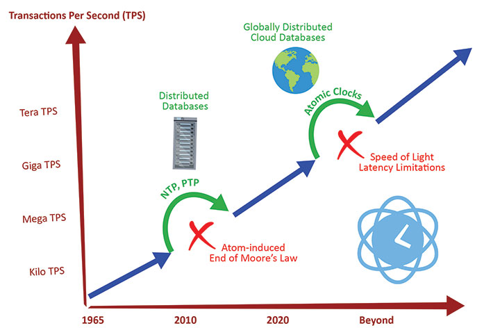
    In 1965, Gordon Moore predicted the transistor count on an integrated circuit would double every year. This was eventually revised to doubling every two years. Along with this increase in transistor density came an important increase in speed as well as decreases in cost and power consumption. 

    It may have been hard in 1965 to imagine there would be any real-world need to have a semiconductor with 50 billion transistors on it in 2021, but as semiconductor technologies kept up with the law, so did application demands. Cell phones, financial trading and DNA mapping are all applications that rely heavily on the number of operations per second a microprocessor can execute, which is closely tied to the transistor count on a chip. 

    Photo:
    Satirical image of an engineer trying to keep up with Moore’s Law. (Image: Microchip Technology)

    The Demise of Moore’s Law

    Unfortunately, Moore’s Law is rapidly coming to an end due to a limit imposed by physics. With wafer fabrication now in the sub-10-nm technology nodes, the transistor sizes are only about 10 to 50 times that of a silicon atom. At this scale, the size and quantum properties of atoms and free electrons significantly prohibit further size reduction. In essence, you could think of the atom as the ultimate court that struck down the law. 

    But while Moore’s Law will come to an end, the thirst for increased processing power will continue to grow. With the advent of the internet of things (IoT), streaming services, social media posts and autonomous self-driving cars, the amount of data generated every day continues to increase exponentially. 

    In 2021, every day an estimated 2.5 exabytes (2,882,303,761,517,120,000 bytes) was generated. Exabyte databases managing more than 100,000 transactions per second (a transaction consists of multiple operations) are currently in use, and the size of the databases and the transactions per second will continue to grow for the foreseeable future.

    Synchronizing the Machines

    This explosive growth in the volume of data — coupled with the speed at which the data must be written, read, copied, analyzed, manipulated and backed up — required data-center architects to find a way around the end of Moore’s Law. The architects employed horizontal scaling in a data center with distributed databases, where instead of an entire database residing on one server, the database is distributed over multiple servers in a cluster. 

    In this configuration, the cluster essentially functions as one giant machine, hence the size and speed of the system now becomes limited by the physical size of a data center rather than by the size of an atom. (Take that, atom!)

    Software engineers now make careers writing code that enables horizontal scaling. For all the software to work, however, all the machines must be synchronized. Otherwise it violates a concept called causality. 

    What is causality? It is easiest to explain through an example. Suppose you have two cameras to record images for a 100-meter dash, each with its own internal clock. The first camera is at the starting blocks. The second camera is at the finish line. Both sensors are continually firing and timestamping each image with the time from their respective clocks. 

    Photo:Clock uncertainty causes issues with causality. In this case, a race officially finished before it started. (Image: Microchip Technology)
    Clock uncertainty causes issues with causality. In this case, a race officially finished before it started. (Image: Microchip Technology)

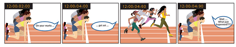
    To determine the official time of the winning sprinter in the race, the first camera’s images are reviewed for the point in time when the first runner left the block and this time-stamp is subtracted from the time-stamp on the last camera’s image for that runner crossing the finish line. 

    For this to work, both cameras must be synchronized to an acceptable level of uncertainty. If the synchronization of the clocks is only ±0.05 seconds, you would be unable to determine if someone who was recorded as running 9.6 seconds actually broke the world record of 9.58 seconds. What if they were only synchronized to ±5 seconds from the stadium clock? 

    Imagine this scenario: Observed from the main stadium clock, a race starts at exactly 12:00:00:00 p.m. The first runner crosses the finish line at 12:00:09:60 p.m. From the perspective of the main stadium clock, the official race time was 9.6 seconds. 

    But what if the first camera’s clock was exactly 5 seconds fast and the second camera’s clock was exactly 5 seconds slow? The race would officially start at 12:00:05:00 p.m and finish at 12:00:04:60 p.m. The race would officially finish 0.4 seconds before it started, the world record would be shattered, the laws of physics would be broken, and the current record holder would most likely be wrongfully dropped by all his sponsors. 

    Applying Causality to a Database

    The same principle of causality is important in a database. Transactional record updates must appear in the database in the sequential order in which they occurred. If you count on the direct deposit of your paycheck arriving prior to having a direct withdrawal to pay your monthly mortgage, and the bank’s database did not record these in the correct sequence, you will be charged an overdraft fee. On one machine, causality errors are easy to prevent, but on multiple servers, each with its own internal clock, the servers must be synchronized and timestamp every transaction.

    To achieve this, one server must act as a reference clock, much like the stadium clock, and it must distribute time to each server in a way that minimizes the time error of each server clock. The uncertainty of each timestamp (±5 seconds in the race) forms a time envelope that is twice the uncertainty of the clock (10 seconds for the race). For a distributed database, the number of nonoverlapping time-envelopes that can fit into a second should be at least on the order of the number of transactions per second expected for the system. 

    Probability, criticality of causality, and cost of implementation will ultimately all play a role in the final solution, but this relationship is a good starting point. A system with time-stamp uncertainties of ±1 millisecond would have time-envelopes of 2 milliseconds, and a maximum of 500 non-overlapping time-envelopes would fit in one second. This system could support approximately 500 transactions per second. 

    Where NTP and PTP Fall Short

    Time-over-Ethernet technologies known as Network Time Protocol (NTP) and Precision Time Protocol (PTP) are used to synchronize all the servers in a distributed database in a data center. These protocols can ensure a local area network can distribute time with sub-millisecond (NTP) or sub-microsecond (PTP) uncertainties, enabling thousands (NTP) or millions (PTP) of transactions per second.

    Unfortunately, even with these solutions that enabled a detour around the atom-imposed demise of Moore’s Law, physics has thrown another roadblock in the path of distributed databases in the form of the speed of light. 

    Imagine a well-synchronized distributed database operating with PTP in San Jose, California, happily executing 100,000 transactions per second with no causality issues. One of the database architects is sitting in his office in New York and his boss asks him to update a large series of records. 

    The architect wants to be able to exploit his new database to its full extent and show off the system capabilities. He plans on executing 100,000 transactions per second. 

    To update records per the request, he creates a simple transaction that adds the value of one record to a second record only if the value of the first record is greater than the second record. To accomplish this, he must issue a read to both records. His local machine in New York will then compare the values, then send a write command to the second record when needed.

    After completing this, he then wants to execute the next transaction that compares a third value to the new sum. If the new sum is greater than the third record, then the third record is replaced with the sum. He wants to repeat this for 6 million records. Because the database is capable of 100,000 transactions per second, he thinks it will be done in roughly a minute. He tells his boss he will have the records updated in five minutes, then leaves to get a cup of coffee. 

    While drinking his coffee, he reads a story about how the new 100-meter dash record is negative 0.4 seconds which defies the laws of physics, and that the previous record holder is suing the stadium officials because he has lost all his endorsement money. The architect laughs to himself and thinks that the stadium should have hired him as the synchronization expert.

    He comes back to his desk five minutes later and is dismayed to see that his database update has completed fewer than 1,500 transactions. He sadly realizes his mistake and prepares his résumé to send it over to the stadium, where he hopes his PTP deployment won’t have the same problem. 

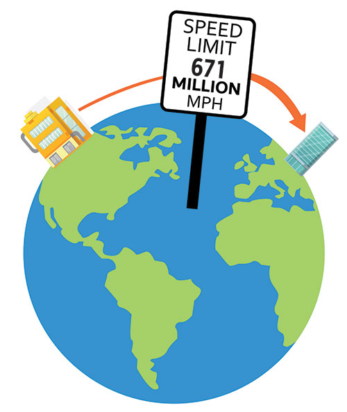
    What went wrong? The speed of light limits the theoretical fastest possible transmission of data between New York and San Jose to 13.7 milliseconds. 

    The speed of light imposes a theoretical limit to the speed at which data can be transferred between two points. (Image: Microchip Technology)
    The speed of light imposes a theoretical limit to the speed at which data can be transferred between two points. (Image: Microchip Technology)

    The Distance Problem

    Unfortunately, real world transactions are even slower. Even with a dedicated fiber-optic link between the two locations, the refractive index of the fiber, the real-world path of the fiber and other system issues make this transit time even slower. So just one transmission from New York will take 40 to 50 milliseconds to arrive in San Jose. 

    However, in this transaction there are four unique operations. There are two read operations, which could happen in parallel, which then have to be sent back to New York. The round trip takes 80 to 100 milliseconds. Then, once both values are compared, a write operation is issued and a write acknowledgement must be sent back indicating the write operation completed before the next transaction can start. 

    Suddenly, it doesn’t matter that the database can perform 100,000 transaction per second, because the distance is limiting the system to 5 transactions per second. To complete the 6 million transactions, this system would take 13 days, more than enough time for several more cups of coffee and to update a résumé. This delay is referred to as communications latency.

    Circumventing Latency 

    But just like with Moore’s Law, database architects figured out how to circumvent latency. Database replications are created near the users, so they can work with the data without having to send signals across the country. 

    Periodically, the replications are compared and reconciled to ensure consistency. During the reconciliation process, the transaction time-stamps are used to determine the actual sequence of transactions, and records are sometimes rolled back when there is an irreconcilable difference such as when the transaction time-envelopes overlap. Reducing clock uncertainty reduces the number of irreconcilable differences in replicated instances, as more time-envelopes reduce the probability of overlaps. This results in higher efficiencies and lower probabilities of data corruptions. 

    But now the timestamping has to be accurate not only within each data center, but also between the data centers, which can be separated by thousands of miles and connected via the cloud. This is a much more difficult task, as it requires an external reference with very low uncertainly that is readily available in both locations.

    Down to the Atomic Level

    Enter the previous foe of the database architect, the atom. While the atom was busy repealing Moore’s Law, its subatomic particles were busy spinning. The neutrons and protons in the nucleus were rotating, while at the same time the electrons were busy orbiting about the nucleus, while also spinning on their own axes. This is analogous to Earth orbiting around the sun while simultaneously spinning on its axis. 

    The electrons can spin around their axes clockwise or counterclockwise. Considering there are roughly 7 octillion (7 with 27 zeros after it) atoms in a human, with all the subatomic particles spinning in our bodies, it is amazing we aren’t permanently dizzy. (Note: The subatomic particles aren’t really busy spinning and orbiting, they are really busy giving us probability wave functions and magnetic interactions that would give us results similar to what would happen if they were spinning and orbiting. But if the thought of all the spinning makes you dizzy, trying to comprehend the reality of quantum mechanics will make you positively nauseous.)

    Conceptual atoms with nucleus and valence electron with nuclear spin, electron spin and orbital spin. (Image: Microchip Technology)
    Conceptual atoms with nucleus and valence electron with nuclear spin, electron spin and orbital spin. (Image: Microchip Technology)

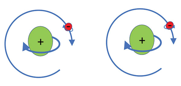
    When microwave radiation at a very specific precise frequency is absorbed by an electron, the direction of spin about the electron axis can be changed. If this happened to Earth, the Sun would suddenly set in the east and rise in the west! 

    Atomic clocks are machines designed to detect the state of the electron spin, and then change that direction through microwave radiation. The frequency varies depending on the element, the isotope, and the excitation state of the electrons. 

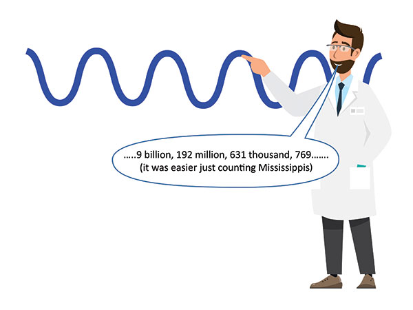
    Once the machine determines the frequency, known as the hyperfine transition frequency, the period can be determined as the inverse of the frequency, and the number of periods can be counted to determine the elapsed time. The international definition of the second is 9,192,631,770 periods of the radiation required to induce the hyperfine transition of an electron in the outer orbital shell of a cesium atom.  

    Atomic clocks are the most stable commercially available clocks in the world. An atomic clock the size of a deck of cards called the chip-scale atomic clock (CSAC) will drift 1 millionth of a second in 24 hours, whereas an atomic clock the size of a refrigerator called a hydrogen maser will only drift 10 trillionths of a second in 24 hours. (Coincidentally, 10 trillionths is also about the ratio of the radius of the hydrogen atom to the height of the sprinters in the 100-meter dash and of the now-unemployed data-center architect in New York.)

    With the accuracy provided by these atomic clocks, approximately 500,000 to ~50 billion non-overlapping time-envelopes can be provided for a distributed database running in data centers in Tokyo, London, New York, Timbuktu or anywhere else in the world.

    The unit second is defined by counting 9,192,631,770 cycles of the cesium hyperfine transmission radiation frequency. (Image: Microchip Technology)
    The unit second is defined by counting 9,192,631,770 cycles of the cesium hyperfine transmission radiation frequency. (Image: Microchip Technology)

    Time for Distribution

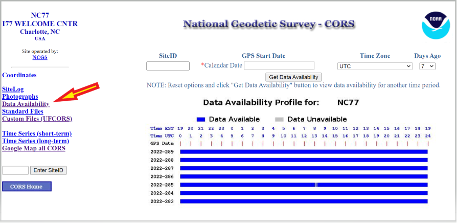
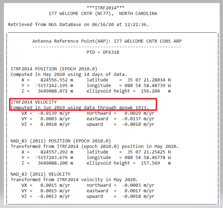
    How does time get to all the data centers from these atomic clocks? Universal Coordinated Time (UTC) is a global time distributed by satellites, fiber optic networks, and even the internet. UTC itself is derived from a collection of high precision atomic clocks located in national laboratories and timing stations around the world. Contributors to UTC receive a report that provides the UTC time from these clocks and their individual offset from calculated UTC. The labs and other facilities then transmit the time to the world. 

    The UTC report is published monthly and tells the national labs their miniscule timing offset from UTC during the previous month. Technically, we don’t know precisely what time it was up until a month after the fact. And to make things worse, extra seconds are periodically added to UTC, called leap seconds, which are inserted due to variations in the Earth’s rotation and our relative position to observable stars. While this aligns Earth to the universe, it causes havoc in data centers and 100-meter dashes. 
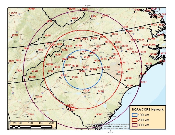
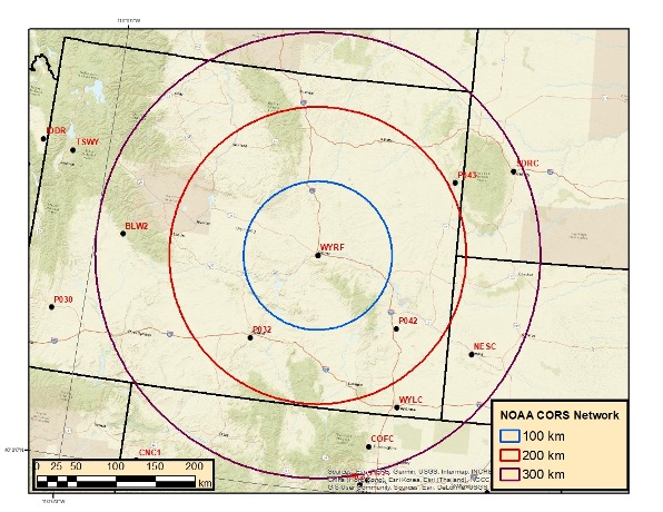
    The hyperfine transition frequency produced in a hydrogen maser, 1.420405751 GHz, will cause spin reversal in an electron. (Image: Microchip Technology)
    The hyperfine transition frequency produced in a hydrogen maser, 1.420405751 GHz, will cause spin reversal in an electron. (Image: Microchip Technology)

    Enter GNSS

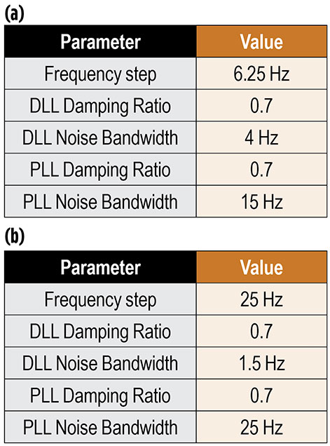
    Two common methods used by data centers to acquire UTC are via the internet using publicly available NTP time servers and via satellite using GPS or other GNSS networks. While timing through public NTP timeservers over the internet was common during early deployment of distributed databases, inherent performance, traceability and security issues have created the push to move away from this solution. 

    Even though GPS and other GNSS are typically thought of as positioning and navigation systems, they really are precision timing systems. Position and time at a receiver are determined by the transit time of signals traveling at the speed of light from multiple satellites to the receiver. Ironically, this is another case of a physics principle causing a problem — in this case the speed of light instead of the atom — but also contributing to the solution. 

    The satellites have their own onboard atomic clocks, which are synchronized to UTC that was transmitted to the satellites from ground stations. Acquiring UTC with this method can provide time uncertainties in the 5-nanosecond range, enabling 100 million time-envelopes per second. 

    This method is far more reliable and accurate than public NTP servers, and while these signals can be interrupted by such events as solar storms or intentional signal jamming, backup clocks that have been synchronized to the satellite signals when present can be placed in each individual data center to provide the desired uncertainty levels during these interruptions.

    The evolution of database transaction rates and the enabling and disabling technologies. (Image: Microchip Technology)
    The evolution of database transaction rates and the enabling and disabling technologies. (Image: Microchip Technology)

    Next Up: Jumping Electrons

    As our quest to acquire, store and transact data in the future continues to grow, novel atomic-clock technologies and time transmission systems with lower uncertainties will be needed. Currently, national timing labs are developing atomic clocks that work on the optical transitions that occur when an electron jumps orbital shells. These offer frequency stabilities to a quintillionth of a Hertz and will eventually be used to redefine the unit second.

    Signal transmission through dedicated fiber-optic links or airborne lasers are already yielding improved transmission accuracy. With these continued innovations data, the atom and light will continue their complex love-hate relationship to enable ever larger quantities of data processed at ever increasing rates without consistency issues or causality casualties. 

  • Seen & Heard: Finding Nemo, weighing bears

    Seen & Heard: Finding Nemo, weighing bears

    “Seen & Heard” is a monthly feature of GPS World magazine, traveling the world to capture interesting and unusual news stories involving the GNSS/PNT industry.


    Photo: Alexey_Seafarer/iStock/Getty Images Plus
    Photo: Alexey_Seafarer/iStock/Getty Images Plus

    HOW BIG IS THAT BEAR?

    Monitoring the weight of polar bears — an important health factor — usually means tranquilizing them from the air and lifting them with a tripod attached to a scale. However, technology might provide a non-invasive solution. Various zoos and sanctuaries are testing the accuracy of lidar scanners to measure the weight of polar bears, reports Geo Week News. The scans could be done using drones and mobile mapping equipment and techniques, according to Joel Cusick, a GIS specialist for the National Parks Service.


    Photo: PaulFleet/iStock/ Getty Images Plus
    Photo: PaulFleet/iStock/ Getty Images Plus

    SLIP SLIDING AWAY

    Researchers used a combination of GNSS and interferometric synthetic aperture radar (InSAR) data from Sentinel-1 satellites to determine subsidence in
    99 cities around the world between 2015 and 2020. Subsidence rates in Tianjin, Semarang and Jakarta exceed 30 mm per year. Even in mostly stable cities, areas are sinking faster than sea level is rising, with Istanbul, Lagos, Taipei, Mumbai, Auckland and Tampa sinking faster than 2 mm per year in some areas. Besides climate change, causes include groundwater extraction, mining, reclamation of natural wetlands, infrastructure projects and ecological disturbances. The study is published in Geophysical Research Letters.


    Photo: NOAA Fisheries/Raymond BolandPhoto:
    Photo: NOAA Fisheries/Raymond Boland

    FINDING NEMO

    National Oceanic and Atmospheric Administration (NOAA) ocean mapping ship Rainier completed a five-month expedition to the Mariana Islands in September, combining mapping and charting with coral-reef ecosystem surveying. Collection of high-resolution mapping data in near real time improved the effectiveness of the traditional marine science data collection as the combined team mapped 4,000 square nautical miles of seabed and conducted 1,800 SCUBA dives. The data will improve navigation safety through updated NOAA nautical charts and increase understanding of coral reefs through the National Coral Reef Monitoring Program. Besides charts, the seabed mapping data supports marine protected areas, sustainable fisheries, and offshore wind siting — and, in the Marianas, is important for tsunami modeling.


    Photo: mikulas1/iStock/Getty Images Plus
    Photo: mikulas1/iStock/Getty Images Plus

    GRAVITY DOWN UNDER

    An airborne gravity sensor is flying above 80,000 square kilometers of New South Wales (NSW), Australia, collecting data that will improve the accuracy of real-world heights from GNSS positioning to just a few centimeters. Data for the 18-month NSW Gravity Model project will be captured in five stages, starting in Western NSW. The resulting model is expected to enable better resource management, infrastructure planning and natural hazard preparation. It is also a critical building block for developing digital twins, replacing datasets that predate GNSS positioning.

  • Research Roundup: Atmospheric effects on GNSS

    Research Roundup: Atmospheric effects on GNSS

    Photo: buradaki/iStock/Getty Images Plus/Getty Images
    Photo: buradaki/iStock/Getty Images Plus/Getty Images

    GNSS researchers presented hundreds of papers at the 2022 Institute of Navigation (ION) GNSS+ conference, which took place Sept. 19–23 in Denver, Colorado, and virtually. The following five papers focused on atmospheric effects on GNSS signals. The papers are available at www.ion.org/publications/browse.cfm. 

    Addressing Scintillation Error

    Mitigating the scintillation effect at low latitude is a complex matter: several kinds of experimental data must be collected, realistic models must be developed, and, most importantly, useful real-time indices and alerts must be made available.

    The authors introduce a prototype based on a patent owned by SpacEarth Technology to address scintillation error detection and mitigation, supporting precision GNSS-based services at low latitudes in any season and space weather conditions. The patent relates to a method of total electron content (TEC) and scintillation empirical forecasting, in particular short-term forecasting (seconds to minutes). The output of the method is necessary to feed mitigation algorithms aiming at improving accuracy on GNSS precise positioning techniques (RTK, NRTK, and PPP) under ionospheric harsh conditions.

    The prototype is designed with a Central Elaborating Facility, which collects the data provided by a network of GNSS monitoring stations detecting scintillation events, and broadcasts foreseen scintillation parameters. Users with a rover mitigation device can apply the parameters from the central facility for scintillation error mitigation. 

    Vincenzo Romano, INGV and SpacEarth Technology; Claudio Cesaroni, INGV; Luca Spogli, Alessandro Fiorini, INGV and SpacEarth Technology; Marco Fermi, Gter; Lorenzo Benvenuto, Gter and University of Genoa; Tiziano Cosso, Gter; Marcin Grzesiak, SRC/PAS; Joao Francisco Galera Monico, Italo Tsuchiya, UNESP; Gabriel Oliveira, Marcos Guandalini; “Ionospheric Scintillation Mitigation at Low Latitude to Improve Navigation Quality.”

    Ring of Fire GUARDIAN 

    Commonly, natural hazards release energy into the Earth’s atmosphere in the form of acoustic-gravity waves, which propagate up to the ionosphere. The resulting traveling ionospheric disturbances (TIDs) can be detected using GNSS signals, through the computation of the integrated total electron content (TEC) along the lines of sight between GNSS receivers and satellites. The global distribution of ground-based GNSS receivers constantly tracking multiple GNSS constellations (GPS, Galileo, GLONASS, BeiDou, and others) provides excellent spatio-temporal coverage around the world, including in areas of limited coverage by existing warning systems.

    The authors present the operational GNSS-based Upper Atmospheric Real-time Disaster Information and Alert Network (GUARDIAN). Based on dual-frequency GNSS data from the Global Differential GPS (GDGPS) network of the Jet Propulsion Laboratory, the GUARDIAN architecture computes slant TEC time series in near real time.

    As part of the GDGPS network, 78 stations around the Pacific ring of fire monitor the four GNSS constellations: GPS, Galileo, GLONASS and BeiDou. Cycle slips are corrected and the time series are filtered, both in real time. The resulting data stream is output live to a user-friendly public website, benefitting the general public and the scientific community. 

    The current GUARDIAN focuses on the Pacific region. However, the architecture can readily be extended to a worldwide coverage.

    Léo Martire, S. Krishnamoorthy, L. J. Romans, B. Szilágyi, P. Vergados, A. W. Moore, A. Komjáthy, Y. E. Bar-Sever, A. B. Craddock, NASA Jet Propulsion Laboratory, California Institute of Technology; “GUARDIAN: A Near Real-Time Ionospheric Monitoring System for Natural Hazards Early Warnings.”

    Civil Aviation Interference

    The authors provide a survey on GNSS receiver architectures with emphasis on new carrier-tracking techniques for mitigating the adverse effect of ionospheric scintillation within the context of civil aviation. The survey is complemented by results gathered from simulations on the impact of ionospheric scintillation in conventional receiver architectures. A review on scintillation mitigation techniques is carried out, covering several “technique families,” highlighting their potential for performance improvement, as well as their shortcomings and challenges in implementation.

    A semi-analytical simulation campaign is carried out for different modulations: L1, L5 for GPS, and E1, E5a for Galileo. Here, the performance of a standard receiver tracking a set of GPS and Galileo satellites affected by ionospheric scintillation is analyzed to pinpoint existing vulnerabilities to this effect.

    The simulation results show that ionospheric scintillations are responsible for large variations in carrier-to-noise ratio, which in turn can be responsible for losses of lock and large phase variations, increasing phase RMSE and in some cases leading to cycle slips of the phase estimation. Thus, the adopted solution must be robust to signal power fluctuations and the occurrence of cycle slips and able to maintain phase lock.

    António Negrinho, GMV-PT Pedro Boto, GMV-PT Marta Cueto, GMV-ES Mikael Mabilleau, EUSPA Claudia Paparini, EUSPA Ettore Canestri, EUSPA; “Survey on Signal Processing Techniques for GNSS Ionospheric Scintillation Mitigation.”

    Tonga Eruption Data Analyzed

    Extreme natural disasters, such as volcanic eruptions, can create visible pressure waves in the atmosphere and trigger observable ionospheric wave responses that can travel hundreds of kilometers in the ionosphere. The acoustic and gravity waves generated can cause ionospheric TEC perturbations and variations. The TEC determines the GNSS ionospheric delay and can cause significant positioning errors, which may affect the performance of GNSS-based applications.

    The researchers processed GNSS data collected from the Hong Kong Satellite Positioning Reference Station Network to analyze the ionospheric activity and positioning performance responding to the Tonga volcanic eruption on Jan. 15, 2022. To detect and repair cycle-slip jumps, the researchers applied theTEC rate and Melbourne Wubbena Wide Lane (MWWL) linear combinations. A Savitzky-Golay low-pass filter with a 30s window was used to improve the TEC accuracy.

    The team investigated the changes in TEC, Rate of TEC index (ROTI) and positioning errors in the eastward, northward and upward directions after the anomalous ionospheric propagation to Hong Kong between 11:30 and 14:30. The team found the ionospheric anomaly could generate large changes in the three parameters, with peaks up to three times the calm period. Their prompt research contributes to a better understanding of the coupling of extreme ionospheric activities and dynamics caused by volcanic eruptions. 

    Xiaojia Chang, Kai Guo, Zhipeng Wang, Kun Fang, Hongxia Wang, Beihang University; Hailong Chen, China Academy of Aerospace Electronics Technology; “Ionospheric Anomaly and GNSS Positioning Responses to the January 2022 Tonga Volcanic Eruption.” 

    Toolbox for Monitor Network

    The MONITORtoolbox is a set of Python-coded software tools to perform automatized large-scale processing of data from the Monitor network of the European Space Agency (ESA). The Monitor network aims to continuously monitor ionospheric scintillation events from multiple ground stations strategically located around the globe. It accommodates a repository with a large number of GNSS measurements containing scintillation events for users to analyze scintillation data or for research purposes.

    This paper shows the potential of the MONITORtoolbox for providing access to a large amount of data that otherwise, without a systematic processing, becomes practically useless. The software developed implements the means to collect data and store it in a local database for quick offline access. It detects the presence of scintillation events based on certain conditions and criteria defined by the user and identifies its properties in terms of duration, time of occurrence, intensity and satellite location. It implements the tools to compute relevant statistics, providing insights on ionospheric scintillation phenomena.

    Sergi Locubiche-Serra, Alejandro Pérez-Conesa, Diego Fraile-Parra, Gonzalo Seco-Granados, José A. López-Salcedo, Universitat Autònoma de Barcelona, IEEC-CERES; Juan M. Parro-Jiménez, Raúl Orús-Pérez, ESTEC, European Space Agency; “MONITORtoolbox — Software Tool for the Analysis of Ionospheric Scintillation Data from the ESA Monitor Network.” 

  • Delivering security through systems engineering

    Delivering security through systems engineering

    Achieving PNT resilience for critical infrastructure applications

    GNSS are magic. They are. One dictionary defines magic as “a power that allows people (such as witches and wizards) to do impossible things by saying special words or performing special actions.” By this definition, we have all become witches and wizards, doing what previous generations would have deemed impossible.

    This magic, however, can be affected by external forces that render it useless at best and, at worst, dangerous. Warnings about GNSS positioning, navigation and timing (PNT) service vulnerabilities have been raised for 25+ years. Numerous organizations have warned of the potential safety, security and economic impacts of GNSS interference. Still, like modern-day Cassandras, their warnings have been ignored, and sole use of PNT services that rely on space-based signals continues to expand.

    “Magic services” are addictive and cannot be ignored. Yet, it is well past the time to merely admire the problem of GNSS interference — benefitting from magical GNSS services while ignoring existing and emerging threats and challenges. It is time to draw a line and implement resilient, complementary PNT solutions to support all critical infrastructure sectors and applications in the event of any GNSS disruption, due to jamming or spoofing or systemic causes. “Magic” is magical when it works. When it does not, first and foremost, it should “do no harm.” 

    Threats, Challenges and Needs 

    Presidential Policy Directive (PPD) 21, Critical Infrastructure Security and Resilience, issued in 2013, defines resilience as “the ability to prepare for and adapt to changing conditions and withstand and recover rapidly from disruptions.” It also notes that “resilience includes the ability to withstand and recover from deliberate attacks, accidents, or naturally occurring threats or incidents.”

    In 2016, the UK Department of International Development noted that “Resilience covers both ‘physical and societal systems” through four “R” principles: robustness, redundancy, resourcefulness and rapidity (see Figure 1).

    Figure 1. Infrastructure resilience properties. (Image: UK Department of International Development)
    Figure 1. Infrastructure resilience properties. (Image: UK Department of International Development)

    More recently, Andy Proctor (RethinkPNT) pointed out that “A resilient PNT system protects its critical capabilities (assets) from harm by using protective resilience techniques to passively resist or actively detect threats, respond to them, and recover from the harm they cause.” 

    Policies, processes, financial arrangements and incentives are also crucial to achieving resilience — and that has been, and remains, the problem. Lacking the emergence of strong leadership from our institutions, the ability to achieve actual resilience will continue to falter and admiration of the problem will continue.

    Developing a resilient PNT system is always a balance of technical complexity and non-technical aspects, for example, costs. The key consideration for users must be the required performance metrics they need for their use-case(s) to ensure their resilience — including accuracy, availability, integrity, continuity and coverage. The one least understood and many times omitted is integrity — the level of trust a user/use-case needs to safely and securely use the PNT services. The ability to trust PNT services must always be a consideration for critical infrastructure applications.

    Unfortunately, many users of critical infrastructure PNT do not know some of the PNT metrics they need to ensure safety and security. More troubling, there is no guidance as to what constitutes “significant economic impact” (see PPD 21) or acceptable economic loss — and over what period or range of use cases. This understanding will require analysis of their design, development and operational experiences, and working with PNT systems engineers to first derive these metrics and then drive the continuous improvements (see Figure 2) needed to achieve and retain truly complementary PNT capabilities. Without clear metrics and guidance, one cannot claim that any solution will meet any “required level of resilience.”

    Figure 2. Resilient PNT lifecycle.
    Figure 2. Resilient PNT lifecycle.

    Supporting PNT Users

    As with all systems engineering (SE) activities, PNT system resilience begins with identifying and documenting user needs based on their specific user stories/use cases. Figure 3 depicts different aspects of resilience that can be sought, depending on the unique use-case “demands.”

    Figure 3. Resilience aspects. (Photo: UK Space Agency)
    Figure 3. Resilience aspects. (Photo: UK Space Agency)

    While the resilience needs of different use cases will differ, for any specific use case, a given “PNT solution” will either achieve the required/threshold level of resilience (based on the operational environment) or it will not. Some use cases may also require fail-safe or fail-soft capability and the ability to recover to known, trusted and usable states. Shouldn’t many, if not all critical sector use cases require this?

    Equally important is the identification of risks and threats, as they are critical to understanding the challenges that the system must face while continuing to provide the necessary P, N and/or T service performance. It is also key to understand and document the system architecture and environment in which it must perform. With knowledge of a user’s needs, the threats, hazards and challenges they face, and the system architecture, the SE process can develop an understanding of the “gaps” that exist and of the levels of risk they impose on a critical infrastructure system’s functional, physical and operational performance. Understanding this, essential use-appropriate mitigations can be identified, or if need be, developed, and a resilient, solution-agnostic PNT requirement document created.

    The Way Forward

    The Critical Infrastructure Resilience Institute (CIRI), a U.S. Department of Homeland Security Center of Excellence, notes that “critical infrastructure systems are facing a myriad of challenges. Solutions must address the cyber, physical and human dimensions.” They keyed into four areas where critical infrastructure resilience activities should be directed: building the business case, information policy and regulation, developing new tools and technologies, fostering and educating the workforce.

    These include the recognition that “policy and regulation have a powerful impact on market forces.” While the fact that “most U.S. infrastructure is owned and operated by the private sector” is a challenge, it should not be an excuse.

    We must start immediately to re-establish strong SE practices, policies, and principles to help critical users understand their needs and determine the metrics required to ensure safety and “preclude significant economic impact.” Only then can we understand from a national perspective, the needed safety and security metrics and what constitutes significant economic impact, and then establish categories of solution-agnostic requirements. Lacking these clear resilience targets, detailed planning, and required resource commitments, the growing threats of PNT vulnerability will continue only to be admired, rather than be mitigated. Hope is not a strategy, but this systems engineer hopes that it does not take a truly catastrophic event to finally prompt much needed and long overdue actions. 


    Mitch Narins is the principal consultant/owner of Strategic Synergies LLC, a consultancy he formed following more than 40 years of U.S. government service. He is a Fellow of the Royal Institute of Navigation, a aenior member of the Institute of Electrical and Electronic Engineers, a member of the Institute of Navigation and head of its Washington, D.C., section, and a member of RTCA, RTCM, IEEE and SAE Standards Committees.

  • Brazilian operator adopts 5G high-precision protocol with Microchip Technology

    Brazilian operator adopts 5G high-precision protocol with Microchip Technology

    Microchip LogoTIM Brasil’s partnership with Microchip Technology provides the accuracy needed for high-performance network architectures, enabling more efficient data transmission

    Now that it has implemented 5G coverage in all Brazilian state capitals, network operator TIM Brasil has enabled precision time protocol (PTP) in its commercial 5G service.

    To accomplish this, TIM has partnered with Microchip Technology, supplier of the TimeProvider 4100 technology, which allows full compatibility and meets the stringent synchronization requirements of 5G mobile network standards.

    PTP allows precise synchronization and times that can reach nanoseconds among cellular base stations, with security of the data transmitted, by encryption.

    Signal synchronization is essential for a successful 5G consumer experience, ensuring better performance, including reduced latency, more accuracy and better transmission quality.

    “The evolution of the 5G offer by the operator does not occur only in the expansion of coverage, but in the possibility of providing the evolution of the service to the consumer,” said Marco Di Costanzo, network director at TIM Brasil. “We want TIM customers to be able to enjoy 5G networks with the best possible experience.”

    He added, “We are satisfied with the easiness of management and robustness of the new TimeProvider 4100, perceived during our extensive field trials, and we are confident this is a perfect match for the demanding requirements in our mobile deployments. It’s a robust synchronization platform, with high scalability, capacity and flexibility for future growth needs.”

    Tests of the new technology were carried out after TIM’s implementation of 5G networks in Brazilian state capitals, and prove the evolution of the service already used by TIM in its partnership with Microchip for the last 10 years.

    The application of the TimeProvider 4100 technology can have a positive impact on the reduction of latency time and can help improve the signal distribution in indoor networks.

    “Our TimeProvider 4100 offers a robust solution with the flexibility to deploy in a wide range of environments accommodating standards required for mobile 5G implementations due to its impressive versatility,” said Randy Brudzinski, corporate vice president for Microchip’s Frequency & Time Systems business unit. “The device uniquely provides a 1588 grandmaster supporting these standards with the high-precision, accuracy and reliability requirements needed for leading mobile operators like TIM Brasil.”

  • Innovation: Software-defined radios for GNSS

    Innovation: Software-defined radios for GNSS

    A Step-by-Step Exposition of an Educational Resource

    Innovation Insights with Richard Langley
    Innovation Insights with Richard Langley

    THE RADIO. It’s been around for more than 100 years. Pioneering work by Guglielmo Marconi and others in the1890s and 1900s resulted in practical wireless telegraphy devices that permitted point-to-point communications with ships at sea and between stations on land hundreds and thousands of kilometers apart and even between stations on different continents. The first radio broadcasts (point-to-multipoint) were time signal transmissions and weather broadcasts. Experimental audio transmissions took place in the early 1900s, and by 1920 or so, radio stations were established in many countries for broadcasting speech and music to the general public.

    The first radio receivers were simple crystal sets. It wasn’t until the mid-1920s that tube radios became commercially available. Eventually, tubes were replaced by transistors, and transistors by integrated circuits. The introduction of microprocessors resulted in digital receivers, with the conversion of the received analog radio signals into audio being carried out digitally for the most part.
    One of the latest advances in radio technology is the software-defined radio or SDR. An SDR typically consists of two components: a piece of hardware, called a radio frequency (RF) front end, and a piece of software run on a general-purpose computer. The job of the front end is to convert a portion of the radio spectrum received by its antenna to a digital data stream processed by the software. The software decodes the data to produce the desired result. Since the software does most of the “heavy lifting” in processing a radio signal, it is often called the SDR itself. And by the way, there are SDR transmitters, too.

    It should come as no surprise that SDR technology has come to the GNSS field. In fact, in 2007, the seminal text on GNSS SDRs, A Software-Defined GPS and Galileo Receiver: A Single-Frequency Approach, was published along with the sale of an inexpensive RF front-end in a thumb-drive-sized package that allowed graduate students and others to experiment with a GNSS SDR themselves. And we have covered GNSS SDR developments in this column from time to time, most recently in January 2018 (“The Continued Evolution of the GNSS Software-Defined Radio: Getting Better All the Time”).

    In this month’s column, researchers from the lab that helped produce the SDRs documented in the 2007 book (which is still in print) discuss their development and testing of additional freely available SDR codebases covering all four GNSS (GPS, Galileo, BeiDou and GLONASS). They provide an excellent resource for learning how GNSS receivers actually work.


    By Joan Bernabeu, Nicolas Gault, Yafeng Li and Dennis M. Akos

    With the publication of the book A Software-Defined GPS and Galileo Receiver: A Single-Frequency Approach by Kai Borre, Dennis Akos and their fellow authors, an open-source GNSS software-defined radio (SDR) receiver developed using Mathwork’s Matlab language was made available, together with sample data sets that facilitated the testing process for all interested readers. The first SDR implementation focused on processing the GPS L1 C/A-code legacy signal and served as a starting point for students and researchers in the Radio Frequency (RF) and Satellite Navigation Laboratory at the University of Colorado Boulder, where later activities aimed to improve the software code and add new features as new GNSS signals emerged. As a result, the initial codebase evolved into a complete collection of SDRs capable of processing all GNSS signals from every satellite constellation, with BeiDou’s B1I, B1C, B3I and B2a signals the latest additions. The most recent efforts were dedicated to collecting all SDR codebases, putting them in a common format, and testing them to give an account of their performance. This article describes our efforts, placing special emphasis on explaining the test framework designed to test each SDR, as well as on reporting the adjustments made and the results obtained. GPS test cases have been taken as examples to show how some SDRs were assessed when issues were found in the results they provided.

    OPEN-SOURCE GNSS SDR COLLECTION

    The whole SDR collection has been developed in Mathwork’s Matlab programming language. To run the code and perform tests, users simply require an active Matlab license and the software available on their computer. Once these requirements are met, the user can choose to download any of the available codebases and the corresponding data set to start experimenting. 

    We recommend using version control software to keep track of changes made to the original version of the code. Users should consult the Borre et al. text for further details on running the codebases.

    A total of 12 SDR codebases are aimed at processing each of the GNSS signals (see TABLE 1). All code files for each SDR are organized in the same subdirectories, and most of them have the same filenames. 

    Table 1. All GNSS signals that can be processed by the SDR collection, organized by their corresponding satellite systems.
    Table 1. All GNSS signals that can be processed by the SDR collection, organized by their corresponding satellite systems.

    All SDRs are set to work with a default configuration. They are all run using an init.m script, which collects user settings (input data file path, sampling frequency and so on) from the initSettings.m configuration script. Given this, the first file that users may want to modify is initSettings.m, to define the run settings for a given test. Most of the SDRs operate in an identical way, however some include particular features oriented at exploiting certain characteristics of the corresponding GNSS signal. The GPS L2C SDR, for example, gives the user the option of whether to process the pilot component of the signal.

    The test samples available in the public directory were obtained in accordance with the characteristics depicted in TABLE 2 for every signal. The first two columns from the left show all the signals the SDR collection can process and the central carrier frequency at which they are transmitted. The third column gives the bandwidth selected in the recording process for every signal. This value must match the sampling frequency defined in the initSettings.m file for each SDR. Only three frequency bandwidths can be used to record GNSS data, so as to make the configuration structure more homogeneous across different SDRs. They were selected to ensure similar characteristics for each signal in terms of performance, encompassing most of the signal power for each modulation, but also keeping the recorded GNSS data files within a reasonable size.

    Table 2. Summary of the tested GNSS signals’ center frequencies and the selected bandwidth (BW) for their processing. The common IF for all signals is 20 MHz.
    Table 2. Summary of the tested GNSS signals’ center frequencies and the selected bandwidth (BW) for their processing. The common IF for all signals is 20 MHz.

    All the signals were mixed to a common intermediate frequency (IF) of 20 MHz in the recording process. Both the frequency bandwidth and the IF are fundamental to obtain the expected results from each SDR codebase. These are set in the settings file. The default configuration was validated in the testing campaign explained in later sections, and should only be modified to meet the user’s specific needs, being aware that some SDR performance characteristics may also be affected.

    BASIC GNSS SDR STRUCTURE

    While the general SDR receiver structure is similar across all codebases, each comes with adjustments and/or additions to adapt the code to the format of a specific signal. The general codebase structure can be summarized in four major modules:

    • signal acquisition
    • tracking stage
    • navigation data decoding
    • position, velocity and time (PVT) computation.

    An important remark is that the SDR collection developed is designed to process files of limited duration. The code is designed to use enough data to provide a successful initial acquisition, and then use a single set of satellites for the remaining execution. In other words, there is no extra logic oriented at acquiring or reacquiring satellites after the first acquisition is achieved.

    Signal Acquisition. The design of the acquisition scheme depends on the characteristics of the signal the SDR is aiming to process. There are numerous GNSS signal configurations for each constellation that follow different strategies concerning spreading codes, navigation data and secondary codes, which must be accounted for in the acquisition codebase.

    All codebases follow a fast Fourier transform (FFT) accelerated serial search-acquisition approach to obtain estimates of the signal’s carrier frequency and code delay, where a number of signal replicas are generated iteratively, separated by a defined frequency interval in the frequency domain. All the frequency offsets are arranged in what are known as frequency bins. This frequency separation will be referred to as the frequency step. The latter is inversely proportional to the integration time and tells the maximum error allowed in the carrier frequency estimate, which is half the frequency step. Both the frequency step and the coherent integration time are parameters that have a strong effect in acquisition results, as will be seen below.

    Each local replica is correlated with the input signal to obtain a code-phase estimate. The length of this correlation is the so-called coherent integration time. The maximum correlation measurement from all frequency bins is then divided by the second maximum found. This ratio is called the peak metric and is used in all SDRs to give a measure of the magnitude difference between the maximum obtained and the remaining correlation results. If the peak metric is not high enough, this implies that the maximum is close to other cross-correlation products and so could not correspond to the result obtained after correlating both input and local replica signals with the right code-phase alignment. When the peak metric surpasses the threshold defined in initSettings.m, the satellite is considered to be acquired. 

    It is worth noting that in all SDR implementations the local replica is constructed by concatenating a whole primary code and a block of zeros of the same length. This prevents navigation bit transitions from affecting the correlation results. For example, GPS L2C-CM SDR’s acquisition correlates 40 milliseconds of data with 20 milliseconds of pseudorandom noise (PRN) spreading code followed by 20 milliseconds of zeros (the zero padding technique). 

    Tracking Stage. The tracking stage is oriented at refining and keeping track of the code and carrier estimates provided by the acquisition stage as well as demodulating the navigation data. This is achieved using feedback loops organized in channels, which are typically referred to as tracking channels. There will be as many tracking channels as the number of satellites acquired. Each tracking channel makes adjustments to the corresponding local signal replica for the given satellite, so that it resembles the real received signal as much as possible. When the replica is sufficiently accurate, the tracking loop locks onto the signal, removes the carrier and spreading code components, and starts registering data bit transitions. The task of every tracking channel is to account for signal variations so that they can keep locked on the signal for as long as the satellite is available for use.

    Tracking channels implement two feedback loops, the delay lock loop (DLL) and the Costas phase lock loop (PLL). The former is focused on the signals’ code phase while the latter on the carrier phase. These modules depend on two major parameters that determine the properties of the loop filter: the damping ratio and the noise bandwidth. On the one side, the damping ratio controls how fast the filter reaches the settling stage. On the other side, the noise bandwidth informs the amount of noise allowed in the filter.

    While all SDRs follow similar tracking loop schemes, some signals, such as GPS L2C, need some adjustments to the parameters mentioned above so that they provide the expected results, as we point out later. Tracking results are stored in a Matlab .mat file, but also can be assessed in the plot the tracking stage generates after it finishes processing all the channels.

    FIGURES 1a and 1b show an example of two different tracking results plots, each of which include seven figures. These show the in-phase/quadrature (I/Q prompts), the navigation data bits decoded, the changes in the raw/filtered Costas loop and DLL discriminators, and the early-prompt-late metrics. Note that the plots in Figure 1a suggest the navigation data bits were demodulated successfully. In contrast, in Figure 1b, data bits cannot be distinguished because the tracking stage failed to demodulate the navigation message.

    Figure 1. (a) shows the plot generated for a successful tracking channel. In contrast, (b) illustrates the results obtained when the tracking loop in question did not lock appropriately to the signal and therefore was not able to demodulate navigation data. (Image: Authors)
    Figure 1. (a) shows the plot generated for a successful tracking channel. In contrast, (b) illustrates the results obtained when the tracking loop in question did not lock appropriately to the signal and therefore was not able to demodulate navigation data. (Image: Authors)

    Navigation Data Decoding. This stage extracts the navigation data required by the SDR codebase to compute PVT estimates from the results delivered by the tracking stage. The latter outputs I/Q prompt samples representing data bits, containing the encoded navigation data. The navigation data format for each signal can be found in the interface control document issued by each satellite constellation operator.

    The general process that each SDR implements to demodulate navigation data from I/Q samples is summarized as follows:

    1. detect a preamble within data bits
    2. arrange the bit sequence in the corresponding structures, such as frames
    3. remove secondary code if present
    4. de-interleave and decode
    5. check if the bit stream has errors
    6. extract navigation parameters

    Once navigation parameters are extracted, they are stored and later used by the functions involved in the PVT computation stage.

    PVT Computation. The PVT stage takes the decoded navigation data, computes satellite positions, and solves the geometry problem, whose solution is the receiver’s location.

    As with all the other stages, all SDRs follow the same approach, and use the least-squares method to solve for a position estimate once all the data is available. Position estimates are delivered in both Earth-centered Earth-fixed and east-north-up coordinates.

    Similarly to the tracking stage, the PVT computation stage returns a plot showing some PVT statistics to help the user get an idea of the PVT performance of the test conducted. FIGURES 2a and 2b show an example of two positioning plots obtained for two different data files. 

    Figure 2. (a) shows the plot of a priori, good statistics for the navigation solution; (b) shows a navigation plot for a file that presented a problem affecting the PVT solution. (Image: Authors)
    Figure 2. (a) shows the plot of a priori, good statistics for the navigation solution; (b) shows a navigation plot for a file that presented a problem affecting the PVT solution. (Image: Authors)

    EXPERIMENTAL SET-UP AND TESTING

    In this section, we present the equipment we used in our tests (see FIGURE 3) and detail the process we followed to collect GNSS data, as well as the testing framework designed to exercise the SDR collection. 

    Figure 3: The antenna was connected to the RF port of the USRP. The USRP sampled the analog data delivered by the antenna using the TCXO as the reference oscillator. The resulting sampled data was stored in a Linux-based computer. (Image: Authors)
    Figure 3: The antenna was connected to the RF port of the USRP. The USRP sampled the analog data delivered by the antenna using the TCXO as the reference oscillator. The resulting sampled data was stored in a Linux-based computer.
    (Image: Authors)

    RF Antenna. The device used to sense the RF GNSS signals was a Trimble Zephyr2 antenna, which has enhanced capabilities for multipath minimization as well as low-elevation-angle satellite tracking properties. 

    The antenna was installed on the rooftop of the Ann and H.J. Smead Department of Aerospace Engineering Sciences building at the University of Colorado Boulder.

    USRP and TCXO Devices. An Ettus Universal Software Radio Peripheral (USRP) B200 hardware SDR connected to an IQD temperature-compensated crystal oscillator (TCXO) was used to collect digital samples from GNSS analogue signals sensed by the antenna.

    The B200 device was controlled by means of the USRP hardware driver (UHD) through a computer running a Linux operating system. UHD is a software application programming interface (API) that enables the development of code to manage USRP settings and operation. 

    PC Setup. The PC setup consisted of a Linux computer  with all the required drivers and program dependencies, as well as with Mathworks’ Matlab software installed. Matlab was used to program and automate the data recording process.

    Recording Process. The equipment described in previous subsections was used to record data suitable for each SDR codebase. The process to obtain signal data for all 12 codebases was reduced to eight stages by selecting an adequate frequency bandwidth, as some signals share the same central carrier frequency (see Table 2).

    For each stage, a total of 100 files with 61 seconds of I/Q GNSS data were recorded over a 24-hour time period. The I/Q samples recorded by the USRP were formatted as 8 bit sine carriers. All the data sets recorded are available together with a description file based on the Institute of Navigation’s metadata standard for GNSS.

    TESTING FRAMEWORK

    The workflow we followed to test every codebase from the collection is outlined in the following steps:

    1. Record data samples. A set of one hundred files were recorded with 61 seconds of GNSS data.
    2. Debug the SDR with the selected files. A debugging stage preceded every test case to ensure the codebase performed well enough, or else to make the required adjustments.
    3. Run the SDR for one hundred trials. A total of one hundred tests, one per file, were performed for all SDRs.
    4. Log metrics and present results. The results from all SDR stages (acquisition, tracking and data demodulation) were stored for each file. Also, each iteration returned a message that summarized the execution results.

    All of the messages returned for every file corresponded to one of the cases summarized as follows:

    1. Codebase issue. Message type returned when the codebase failed because of a coding issue.
    2. No navigation solution. The codebase was not able to deliver a navigation solution either due to a malfunction of the codebase or due to a lack of satellite availability. Navigation solutions are only available when both the tracking channel and the navigation data demodulation stages are successful for more than three satellites.
    3. Navigation solution with accuracy worse than 30 meters. A position solution fix more than 30 meters (in three dimensions) from the known antenna location was considered a non-accurate estimate.
    4. Navigation solution with accuracy under 30 meters. When the 3D positioning error was < 30 meters, the navigation solution for the position was considered accurate.

    All codebases passed a debugging stage before being tried with the whole set of available data. This was done to ensure that they performed as expected, and were able to achieve the required performance in terms of the metrics mentioned above in this section. An example of this debugging stage will be explained in further detail below. We take the GPS L2C codebase as an example of how all implementations were assessed in an attempt to improve their initial performance and make them more robust to code errors. See our proceedings paper for further details of our test cases.

    GPS L2C Test Case. The problem observed for GPS L2C was that some satellites acquired with a high acquisition metric were failing the tracking stage. The result was that no navigation data was demodulated from them. An in-depth study was required to find out the adjustments needed in the codebase that would help to solve this issue.

    The GPS L2C signal encompasses two signal components called civil moderate (CM) and civil long (CL). The CM component is formed by a spreading code that modulates a navigation message. The CL component is a pilot (data-less) signal modulated with a longer spreading code allowing for longer coherent and non-coherent integration times, yielding better sensitivity. 

    For CM signal acquisition, the 20 millisecond code length limits the coherent integration time to 20 milliseconds, due to the overlaid navigation message. This integration time defines the minimum frequency resolution required to obtain the expected correlation results. The CL component is used in the SDR to accumulate consecutive correlation results non-coherently, contributing to the receiver’s sensitivity by allowing it to operate with higher acquisition metrics in general.

    The initial configuration for this SDR codebase is represented in TABLE 3a.

    Table 3. Configurations for GPS L2C test case.
    Table 3. Configurations for GPS L2C test case.

    With this configuration, a total of 10 satellites were acquired. However, it was observed that for some satellites acquired with high peak metrics, it was not possible to demodulate their navigation data, and thus they were not considered for the navigation solution in later stages. This situation was abnormal, as typically this behavior is more characteristic of weaker signals whose bit transitions are too noisy to be decoded. This problem suggested that either the code-phase or the carrier frequency estimates (or both) were not accurate enough for each tracking channel to generate a proper replica to lock onto the input signal.

    The first step taken to address this matter was to inspect the SDR’s acquisition stage for a file presenting the mentioned problems. For instance, taking a closer look at the carrier and code-phase 3D representation for those satellites acquired with a high acquisition metric that were not successfully tracked afterwards. After doing so, some satellites were identified with the irregular characteristics described above, as for example the PRN 10 satellite. PRN 10 is taken as a reference throughout this subsection.

    The metric analyzed for PRN 10 was the matrix built by the acquisition’s serial search process. This matrix contains the correlation results obtained for each frequency bin. The width of each frequency bin is determined by the frequency step size defined in the configuration file. In this way, the smaller the frequency step, the more frequency bins that the corresponding matrix contains. This implies a better frequency resolution. 

    With this in mind, the frequency resolution was progressively increased by decreasing the frequency step size. Extra logic had to be added to the acquisition algorithm to implement this feature. It was found that when using a step size of 6.5 Hz, the tracking stage was then able to lock and demodulate navigation bits from PRN 10 effectively. This was the most significant determining factor to overcome the issue in question for the majority of the satellites available. However, other smaller adjustments also improved tracking results in general. These are depicted in TABLE 3b.

    CODE AVAILABILITY

    All the resources concerning the SDR collection are publicly available at the portal hosted by University of Colorado Boulder. Through this portal, all the GNSS codebases along with the data sets for testing can be acquired, as well as access to the discussion forum.

    CONCLUSION

    The first version of the SDR collection was made available after the seminal text by Borre et al. was published and consisted of a GPS L1C/A SDR and multiple data sets. From then on, this project kept evolving by adding more SDRs as new GNSS signals emerged across different satellite constellations.

    Our most recent work was to collect all the SDR codebases, arrange them in a common format, and test each implementation to assert their robustness and extract statistics concerning their performance.

    Future work will be dedicated to adding more features aiming at refining the PVT estimates delivered by each SDR.

    More progress is expected to be made soon, with additional improvements made in the GNSS laboratory. In addition, there is plenty of room for contributions from other researchers who want to support and collaborate with this open-source initiative. Our portal provides a convenient way to manage these contributions.

    ACKNOWLEDGMENTS

    We thank the many individuals who collaborated in the development of the open-source GNSS SDR collection. 

    This article is based on the paper “A Collection of SDRs for Global Navigation Satellite Systems (GNSS)” presented at ION ITM 2022, the 2022 International Technical Meeting of the Institute of Navigation, Jan. 25–27, 2022. 


    JOAN BERNABEU is a Ph.D. student at the Institut Supérieur de l’Aéronautique et de l’Espace, Toulouse, France. He also works as a satellite navigation engineer for GMV, Spain.

    NICOLAS GAULT is a Ph.D student at École Nationale d’Aviation Civile, Toulouse, France. He was a visiting scholar in the Department of Aerospace Engineering Sciences at the University of Colorado (CU) Boulder in 2020-2021.

    YAFENG LI is an associate professor in the School of Automation at the Beijing Information Science and Technology University, China. He was a visiting researcher with the Department of Aerospace Engineering Sciences, CU Boulder in 2017–18.

    DENNIS M. AKOS is a faculty member in the Department of Aerospace Engineering Sciences at CU Boulder.

  • Launchpad: Rescue beacon, satellite imagery, z-axis positioning

    Launchpad: Rescue beacon, satellite imagery, z-axis positioning

    A roundup of recent products in the GNSS and inertial positioning industry from the November 2022 issue of GPS World magazine.


    OEM

    GNSS Module

    For UAV, precision agriculture and autonomous machines

    Photo: Unicore Communications
    Photo: Unicore Communications

    The UM982 GNSS module is a high-precision, dual-antenna real-time kinematic (RTK) positioning and heading module. It supports BeiDou B1I/B2I/B3I; GPS L1/L2/L5; GLONASS L1/L2; Galileo E1/E5a/E5b, QZSS L1/L2/L5; and SBAS in dual-antenna mode. The highly integrated, compact (16 mm × 21 mm × 2.6 mm) module can reduce the design area of an OEM board by 72% compared to previous modules. Power consumption is less than 0.6 W. The NebulasIV GNSS system-on-chip is a key part of the UM982’s navigation system. The NevulasIV integrates RF, baseband and high-precision algorithms on a single chip, with supporting functions built in. High-level performance indicators include raw observation accuracy, RTK positioning accuracy, precise point positioning accuracy, and time to first fix. The two antennas can independently participate in deriving an RTK solution and outputting the positioning results.

    Unicore Communications, en.unicorecomm.com

    GNSS Antenna

    Alternative to ceramic patch provides omni-directional performance

    Photo: Antenova
    Photo: Antenova

    The Agosti (part number SR4G080) is a new miniature surface-mount-designed (SMD) antenna for GNSS applications. It measures 9.0 mm x 5.8 mm x 1.7 mm and operates with exceptional efficiency in a reduced space on a corner of a printed circuit board. It has a small ground-plane requirement of 40 mm x 20 mm, 70 mm x 25 mm and 80 mm x 30 mm, making it suitable for small form-factor designs such as wearable devices, trackers and onboard diagnostics.

    Antenova, antenova.com

    Timing Antenna

    Housed Dual-Band antenna with Accutenna technology

    Photo: Tallysman
    Photo: Tallysman

    The dual-band TW3885T antenna supports GPS/QZSS L1/L5; Galileo E1/ E5a/b; BeiDou B1/B2/B2a; GLONASS G1/G3; and satellite-based augmentation systems in the region of operation: WAAS (North America), EGNOS (Europe), MSAS (Japan) or GAGAN (India). It is housed in a through-hole mount, weatherproof (IP69K) enclosure. It mitigates the effects on GNSS receivers of new signals or harmonic frequencies from adjacent LTE bands on the radio-frequency spectrum. For permanent installations, L-bracket (PN 23-0040-0) or pipe (23-0065-0) mounts are available. Tallysman provides an antenna installation guide that recommends a 100 mm –125 mm ground plane and provides antenna installation and cable connector waterproofing best practices.

    Tallysman Wireless, tallysman.com

    Front End

    Simplifies product development for high-precision applications

    Photo: Taoglas
    Photo: Taoglas

    The TFM.110A is the first in a new series of high-precision, multi-band GNSS front ends for autonomous vehicles, precision agriculture, automotive applications and robotics. It comes fully integrated with two cascaded low noise amplifiers (LNA) and pre-filters in a small, low-profile, shielded surface-mount package. When used between the device’s GNSS receiver and antenna, the two-stage amplifier solution eliminates the need for complex and challenging onboard filter and amplifier circuits. It supports L1, L2 and L5 bands and enables seamless signal transmission, signal purity and position accuracy in high-precision applications.

    Taoglas, taoglas.com


    SIMULATORS

    Signal Simulator

    Provides interference, spoofing, encryption and authentication capability

    Photo: IFEN GmbH
    Photo: IFEN GmbH

    Version 2.8 of the NCS Nova RF signal simulator offers advanced capabilities. With integrated interference generation capability, the Nova can generate coherent interference signals with a signal power of up to –30 dBm. The ability to assign two users to one RF output enables integrated spoofing scenarios with a single RF output, meaning spoofing is available even with an entry-level single RF Nova. The new release has advanced navigation message authentication simulation capability compliant to User ICD 1.0 for the Galileo E1-B OSNMA, meaning specific OSNMA events can be simulated — key to ensuring compliant receiver behavior. Supported events include renewal and revocation of both a public key and a TESLA keychain. GPS cross-authentication and generation of Galileo E6-C encrypted codes are also supported.

    IFEN GmbH, ifen.com


    MOBILE

    Z-Axis Positioning

    Enables first responders to locate callers on floor levels

    Photo: Polaris Wireless
    Photo: Polaris Wireless

    Z-axis location service enables the pinpointing of a smartphone user within one floor level inside a multi-story building. The technology — demonstrated to meet the 3-meter vertical location accuracy requirement of the Federal Communications Commission (FCC) — is integrated into Schok Gear’s newly released flip phones. The Schok phones provide consumers with a simple, powerful device. Adding indoor and vertical location to these phones enables first responders to locate all wireless 911 callers with floor-level accuracy in multi-story buildings.

    Polaris Wireless, polariswireless.com

    Rescue Beacons

    Connected with free mobile app

    Photo: ACR Electronics
    Photo: ACR Electronics

    The new ACR Electronics GlobalFix V5 Emergency Position-Indicating Radio Beacon (EPIRB) and ResQLink AIS Personal Locator Beacon (PLB) have integrated the automatic identification system (AIS) to increase the speed of location and aid. They also are compatible with Return Link Service (RLS) alerting. The combination of services ensures faster rescue and increases chance of survival of both boat (EPIRB) and crew (PLB). The safety beacons deliver mobile connectivity to a cell phone with a free mobile app, made possible with the addition of near-field communication technology in the beacons. With the app, users can monitor their beacons, review self-test results, view GNSS test locations, and monitor beacon performance and maintenance by scanning the beacons with their mobile phones. Besides GNSS positioning, the lightweight beacons have 406-MHz Cospas-Sarsat distress signal with MEOSAR compatibility and 121.5-MHz local homing signal.

    ACR Electronics, acrartex.com

    Device Management Platform

    For Internet of Things deployments

    Photo: Laird Connectivity
    Photo: Laird Connectivity

    The Canvas Device Manager simplifies workflows for configuration and maintenance of internet of things (IoT) device deployments. It enables users to easily set up devices, monitor performance, and keep software up-to-date across the entire IoT device fleet. Device parameters can be remotely managed, and performance monitored. Canvas enables users to organize large numbers of devices to quickly build and maintain IoT solutions, and software updates can be remotely and rapidly deployed, thwarting security attacks.

    Laird Connectivity, lairdconnect.com


    SURVEYING & MAPPING

    Slim Receiver

    Advanced technologies in a slim, portable unit

    Photo: ComNav
    Photo: ComNav

    The N2 Palm RTK GNSS receiver is suitable for surveying, mapping and construction. It has a highly integrated main board and a three-in-one antenna, yet weighs 0.72 kg with battery and measures 48 mm. Powered by ComNav’s SinoGNSS K8 high-precision module, the N2 can track 1,590 channels, including all existing and planned signals of GPS, BDS-2, BDS-3, GLONASS, Galileo, QZSS and SBAS. Its advanced satellite-tracking technology ensures it works well even in harsh environments, such as under heavy foliage or close to buildings. A third-generation inertial measurement unit (IMU) makes the N2 immune to magnetic disturbance, which greatly improves its reliability. Pole-tilt compensation of up to 60° allows surveyors to locate points within 2.5 cm. By using the company’s Quantum algorithm, the N2 achieves calibration-free operation — after 10 seconds of initialization, users can make tilt measurements with centimeter-level accuracy for an extended period, greatly improving efficiency.

    ComNav Technology, comnavtech.com

    Image Library

    Now with Pléiades Neo 30-cm imagery

    Photo: Airbus
    Photo: Airbus

    Airbus has added 30-cm Pléiades Neo imagery to its OneAtlas Living Library service. The new data source will complement the service which already allows users to instantly access a premium catalogue of Pléiades 50 cm and SPOT 1.5 m data via streaming, download and API. The Living Library provides frequent updates over urban areas, airports, harbors and military sites to name a few. Imagery is updated every day and processed in the cloud, with flexible options for integration into GIS workflows. With the OneAtlas Living Library, Airbus offers a pay-per-order option but also a subscription-based service that allows users to access premium content quickly available into their account, as well as a deeper archive of more than 10 years of imagery by Pléiades and SPOT satellites at a higher incidence angle and cloud coverage threshold, which will be available in just a few hours. OneAtlas also provides access to several other data services, such as reactive tasking, that allows users to task a full suite of optical and radar satellites, including Pléiades Neo, or access more than 15 years of global radar data, as well as the ability to download the WorldDEM product suite among others.

    Airbus, https://oneatlas.airbus.com/service/living-library

    Satellite Imagery 3

    Free, user-friendly tool shows the Earth’s changes

    Photo: Kermap
    Photo: Kermap

    The Nimbo Maps platform provides monthly 10 m-resolution images of changes on Earth in a user-friendly format. The images are chronological, seamless and free of clouds, and include intuitive comparison timelapse features. The platform, developed by French startup Kermap, relies on innovative artificial intelligence methods to process satellite images supplied by the European Union’s Copernicus program through its Sentinel missions. APIs automatically retrieve data extracted from satellite imagery, providing Kermap customers with real-time, strategic, value-added information in the fields of agriculture, land planning and environmental transitions. Current coverage includes Europe, the Middle East and the United States, with plans to provide global coverage by early 2023.

    Kermap, www.kermap.com; Nimbo, nimbo.earth

    3D Imaging System

    A lightweight payload package

    Photo: GeoCue
    Photo: GeoCue

    The TrueView 655/660 3D imaging system uses the Riegl miniVUX-3UAV laser scanner and three fully integrated mapping cameras (right, left and nadir) for high-accuracy mapping with excellent vegetation penetration and wire detection. Previous TrueView 3D systems carried dual oblique cameras to maximize mapping coverage. The TrueView 655/660 adds a third RGB camera, allowing for imagery directly below the sensor to be captured. The third camera provides a direct view of the ground below to maximize data collection for time flown, while improving the quality of photogrammetry and colorized point clouds.

    GeoCue, geocue.com

  • GPS interference harms the economy, national security and everyday people

    GPS interference harms the economy, national security and everyday people

    GPS relies on faint radio signals from satellites about 12,000 miles away, requiring a quiet spectrum neighborhood to operate. (Photo: NASA)
    GPS relies on faint radio signals from satellites about 12,000 miles away, requiring a quiet spectrum neighborhood to operate. (Photo: NASA)

    By Alex Damato
    Acting Executive Director
    GPS Innovation Alliance

    From its humble beginnings in the 1970s to its expanded use in the present day, GPS technology has been vital for nearly every industry from defense and aviation to farming and construction. GPS devices are designed to receive faint GPS signals transmitted from satellites about 12,000 miles away. Acknowledging this reality, regulators have historically maintained for GPS, which relies on such faint radio signals and sensitive equipment, an appropriately quiet spectrum neighborhood—populated by similar users.


    With the NASEM report’s confirmation of harmful interference, the deficiencies of the FCC’s April 2020 decision are even more striking


    Although these GPS signals and equipment have benefitted from decades of optimization, it is impractical to place highly sensitive GPS receivers designed to capture faint signals from remote transmission facilities immediately next to high-power communications equipment. Unlike those from communications systems, GPS signals are below the thermal noise floor when they are received. As a result, increases in that noise floor often decrease the availability of GPS services, which in turn places at risk high-consequence and safety-of-life services that rely on GPS.

    Alex Damato
    Alex Damato

    Why does this matter? In April 2020, the FCC approved a plan to deploy a terrestrial network in spectrum adjacent to the frequency bands used by GPS — operating communications signals that would be around two billion times more powerful than GPS signals at the same location.

    This past September, the National Academies of Sciences, Engineering, and Medicine (NASEM) released a report detailing the harmful effects of a terrestrial communications network that would operate in a frequency band close to that of GPS.

    Expert concern within 14 federal agencies and departments, a broad coalition in Congress, and the GPS industry resulted in a congressional mandate that NASEM conduct an independent technical review of potential interference to GPS. After a thorough review of the materials, NASEM concluded that the proposed terrestrial network would result in harmful interference to a substantial number of GPS receivers.

    In particular, the report noted that high precision GPS devices, which are used in the most economically significant GPS applications, are the most vulnerable receiver class and likely to be affected by interference. The potential for any interference with GPS, especially with devices used by the Department of Defense, poses a threat to national security, the economy, and our daily lives.

    With the NASEM report’s confirmation of harmful interference, the deficiencies of the FCC’s April 2020 decision are even more striking: potentially millions of farmers, pilots, construction companies, and first responders may be required to repair or replace GPS equipment at their own cost. Although the FCC assumed that this equipment could be repaired through upgrades or filters, some devices cannot be filtered without significant financial and performance costs, and some devices simply cannot be filtered at all.

    GPS is estimated to provide up to $300 billion annually in benefits to the economy. Any disruption in GPS accuracy and usage would have detrimental effects on productivity and economic growth. Moreover, the year before the FCC’s flawed decision, another key report revealed that the loss of GPS service would have an average impact of $1 billion per-day on the nation.

    The GPS Innovation Alliance will continue to work with all federal and industry stakeholders to maintain open channels of communication to connect, listen, and learn from all those involved in the discussion. As technological innovation continues, these debates on harmful interference are not going away, and GPSIA is looking forward to engaging further.

  • Seen & Heard: Goodbye to QE2, saving Ukrainian heritage

    Seen & Heard: Goodbye to QE2, saving Ukrainian heritage

    “Seen & Heard” is a monthly feature of GPS World magazine, traveling the world to capture interesting and unusual news stories involving the GNSS/PNT industry.

    Photo:
    Screenshot: Lying in State Queue tracker

    Queue Tracker for the Queen

    After the passing of Queen Elizabeth II on Sept. 8, the British government launched a live queue tracker app to give people an idea how long they would have to wait to pay their respects at her lying in state at the Palace of Westminster. The app also used What3Words to help locate the end of the line using a three-word tag. The queue grew dramatically in the days before the funeral as tens of thousands lined up, some waiting as long as 16 hours. The app also showed locations of public toilets, drinking water and first-aid stations along the queue route.


    Lake Sarez. (Photo: Astronaut Photography Collection/NASA)
    Lake Sarez. (Photo: Astronaut Photography Collection/NASA)

    A Dam Problem Solved

    Lake Sarez, deep in the Pamir mountains of Tajikistan, was created only a century ago when a strong earthquake triggered a massive landslide. The area experiences considerable seismic activity, which could result in massive flooding downstream should a landslide dam break. With the help of 40 donkeys, 10 scientists and 30 staff from the National Time Service Center of the Chinese Academy of Sciences transported and installed a BeiDou-based deformation monitoring system at the dam. The team had to resolve technical problems in the rugged area, such as providing sufficient solar power and communications. With the system now operating, the dam is being monitored in real time down to the millimeter.


    Figure 3. (Image: CC BY 4.0, Remote Sensing 14, no. 17: 4274) Photo:
    Figure 3. (Image: CC BY 4.0, Remote Sensing 14, no. 17: 4274)

    Counting the Forest for the Trees

    Integration of aerial and ground-based mobile mapping sensors and systems is enabling a team of Purdue digital forestry researchers to locate, count and measure more than a thousand trees in a matter of hours. “The quick, accurate inventory of the global forest ecosystem will improve our ability to prevent forest fires, detect disease, perform accurate carbon counting and make informed forest management decisions,” said Songlin Fei, the Dean’s Remote Sensing Chair. The Purdue-made systems integrate GNSS and inertial navigation devices with lidar and cameras, deployed with manned aircraft, drones and backpack-mounted systems. The technology gathers a variety of information about each tree, including height, trunk diameter and branching formation. The team maintains the precise location and time tags of all acquired features.


    Photo: Skeiron
    Photo: Skeiron

    Saving Ukranian Heritage

    By the end of May, at least 367 incidences of destruction had occurred to Ukraine’s museums, churches, theaters and libraries. Through the project #SaveUkranianHeritage, mapping company Skeiron is capturing sites in high detail using laser scanning and photogrammetry. For a UNESCO-protected church in Lviv, the team gathered more than 300 individual laser scans and 6,000 photos to create a 3D model. The company has two laser scanners — a Leica C10 and Leica ScanStation P20, DLSR cameras and a drone. To support the project with funding or equipment, visit skeiron.com.ua/en/saveukrainianheritage/.

  • Seeking machine control ubiquity

    Seeking machine control ubiquity

    Guidance and precision control, the base elements of modern machine control for construction, have continued to evolve since broad productization began in the mid-1990s. However, the value proposition has become even sweeter since, with value being realized beyond the return on investment (ROI) of the general contractors and the total project price tag for the clients. While the majority of equipment globally is still non-digital, new levels of simplicity and affordability are helping to fill that gap.

    The roots of machine control stretch back a century. The Historical Construction Equipment Association (HCEA) posits that the A.W. French & Co. “utility grader” of the 1920s, a crawler-mounted unit that used stringline control, may be the very first example — and this before electronics and computing. However, it was the advent of real-time kinematics (RTK) for GPS in the mid-1990s that brought machine control as we know it to the construction site, and coincidentally to precision agriculture.

    Initially, the focus was on guidance. Then it moved to precision control, such as blade control, and later propagated to more classes of motorized equipment, improved with further sensor integration.

    The impact on construction and agriculture has been undeniable: productivity gains, less rework, more efficient handling of materials, shorter timelines, site safety improvements, and more. These benefits are as obvious to clients and operators as they were in the early days of adoption, gains from nearly three decades of innovation.

    What form have these growing benefits taken, and who is realizing them? We sought insights from industry experts to find out.

    Grading and Excavation

    Automation is not just about speed; it is also about better control of the load and stress on the equipment and moving just the right amount of materials so as not to place a burden on it. Photo: CHCNav
    Automation is not just about speed; it is also about better control of the load and stress on the equipment and moving just the right amount of materials so as not to place a burden on it. (Photo: CHCNAV)

    These two activities, as each of our interviewed experts attest, represent the lion’s share of realized productivity gains.

    While not the complete picture of overall value, the sheer volume of equipment that has been, or could be, automated speaks, well, volumes. “Apart from the skid steer systems, there are more excavators manufactured than all the other equipment types combined,” said Daniel Sass, product manager of machine control at Hemisphere GNSS. “Excavators are the workhorse. And people use them differently, and they use other pieces of equipment to complement excavators somewhat differently. Certainly, the bulk of our sales is excavators, and in fact a key part of our value proposition is focused on compact machines, but also all the way up to mining shovels. Certainly, by volume it is excavators and compact excavators.”

    Numbers help tell the story. “In the United States, at least in a three-year period from 2019 to 2022, about 253,000 excavators were sold, for which I have pretty reliable data, but only 61,000 dozers and only 7,000 scrapers,” Sass said. “That’s North America, where we also use a lot of dozers and scrapers. If you go to Europe, where they use excavators for many other tasks, the proportional impact might be higher.”

    Operators can easily gauge the ROI of going digital for individual pieces of equipment such as excavators, but part of the incentive could be that general contractors are requiring subcontractors to be equipped and ready to fit into a more complete digital site. “Some definitely require it,” said Randy Noland, vice president of global sales at Hemisphere GNSS. “A lot of … larger sites. I wouldn’t say everybody mandates it yet, but that it is growing.”

    “Operator assistance is not only helping someone cut to grade faster, but is also the best way to cut to grade,” said Cameron Clark, earthmoving industry director, Trimble Civil Construction. “How do you move the material? That directly ties into productivity by only moving the material you need to move, which also equates to less fuel because you can do it faster.” With operator assistance, Clark said, it is not uncommon to see productivity gains of 30% to 40%, even with inexperienced operators. And with automatics, this could exceed 75%, depending on the work done.

    There are substantial gains to be made in operator assistance for less complex heavy equipment, such as compactors. “Often a contactor will put a less experienced operator in the compactor,” Clark said. “In manual days, to overcome the potential of under-compaction and missing spots, they’d create quite a big overlap, maybe up to 40% of overlap between paths. By adding steering control, we can automate the compactor to where it needs to be — to stay on line every day, all day. And you can reduce the overlap to 10% or 15%; having to compact a smaller area means that you’re quicker, say 30% quicker.”

    “Grade control gains can be 30% to 50%,” said Magnus Thibblin, president, machine control division, Hexagon Geosystems. “Depending on the machine and the job application, and how experienced the crew is, it can be similar for excavators.” Thibblin was an end user from the early days of machine control. He saw its potential and how it might work better. Its benefits came not just from automating elements of the equipment, he said, but from implementing a more complete digital workflow.

    “How much are you working with the digital design from the start?” Thibblin said. “I’m one of those who believes you should have 3D from the start; for any kind of layer that the machines can build to. Incidentally, in North America, working to models is implemented for a lot of graders and dozers. In Europe, there is a large excavating market, but it’s the same foundation. If you work from the design, you will have savings in fuel, time, efficiency, safety, etc. Depending on all of these things, the total value proposition may be 30% to 70%.”

    Wenming Sun, vice general manager for digital construction, CHCNAV, reiterates these points. “Currently, our machine control solutions are mainly installed on earthmoving machines, including bulldozers, excavators and motor graders,” Sun said. “The greatest value of these solutions is to improve construction efficiency, shorten construction time, reduce fuel consumption and mechanical wear while ensuring construction quality.”

    CHCNAV is a relatively new player in the construction machine control market, launching initially in Europe and Asia. The company has been developing automation and steering systems for equipment that can yield the highest gains for their customers. “For example, our 3D TG63 automatic control system for motor graders can double efficiency compared to manual operation of machines and reduce time by 50% for the same workload,” Sun said.

    Getting to the designed grade, or trench line, of earthworks geometry faster is a huge benefit, while reducing or removing finishing steps is a bonus. “Now we’re seeing that with excavators that have automatics, the finishing we can get out of an excavator is amazing,” Clark said. “You used to get dozers cleaning up after excavators. Now, with the performance you can get with an automatic excavator, you often don’t need to run the dozer — the excavator can get it done the first time.”

    However, dozers are used for many other tasks. Clark noted that about 95% of blade-control systems for dozers sold have automatics. He said grade control brings tremendous productivity gains, but that excavation is right up there as well. “When you look at the number of machines out there, it’s in a different league,” Clark added. “In 2021, for example, globally about 370,000 crawler excavators and 325,000 mini excavators were sold.”

    Lateral Benefits

    GNSS has revolutionized automation for many classes of heavy equipment. However, for certain high precision work, particularly finished elevations, site levels and totals stations are essential. Photo: Hexagon
    GNSS has revolutionized automation for many classes of heavy equipment. However, for certain high precision work, particularly finished elevations, site levels and totals stations are essential. (Photo: Hexagon)

    For the general contractor, ROI is a key measure. This can be reasonably easy to gauge, as this ROI calculator shows: intelligent-construction.com/roi-calculator/. However, what matters is not just the upfront time and cost for grading and excavating, but also avoiding lateral time and costs. “If you can do jobs faster and more accurately, it lends itself to less rework,” Clark said. “You do it right the first time, which again goes into less fuel, and then also less material. For example, let’s say your excavator is digging down to a trench and the operator digs too deep, which happens often. That material dug out of the trench potentially needs to be carted away. So, extra fuel and trucks are needed to take the material away. They’ve got to put high quality material back in, so that means they actually have to cart more material back to put in the trench, and you have to spread the material.

    Again, it’s a flow-on effect — a chain reaction. When you look at sustainability, what we do has direct and indirect effects — it’s 1 gallon of fuel you don’t use that saves about 22 pounds of carbon emissions.”

    The green dividend goes beyond just what individuals and firms wish to see. Increasingly, infrastructure developers and owners may be subject to sustainability requirements. Depending on where the work is being done, sustainable development goals are being acted on. This includes not just the environmental goals, but also requirements for the digitalization of design and construction, and ultimately smarter and more sustainable infrastructure. Machine control in construction can deliver some of the most substantial benefits in meeting these goals.

    Like overall value for the operators and clients, gauging the highest green dividend becomes a proposition of sheer volume. “On average, your dozer is going to burn much more fuel. However, we sell four times as many excavator solutions as we do for dozers,” said Miles Ware, vice president of marketing and global customer care, Hemisphere GNSS. “The excavator solution is critical for both an ROI and an environmental impact.” Among the most-sold excavators in the United States are the Kubota 4-ton, the John Deere 3.5-ton and 5-ton, and the Caterpillar 5-ton. “The smaller excavators are going to use a lot less fuel,” Ware added. “If we compare this to mid- and large-sized excavators and dozers, we might be getting close to a point of equilibrium, when it comes to environmental impact. Those that consume huge amounts of fuel move massive amounts of earth. However, the ability to have the larger units operate much more efficiently, complete jobs much faster, and get on site and off site quicker with fewer passes in fewer hours adds up to a green dividend. Then you take the smaller volumetric scale of so many excavators and the environmental benefit really starts to balance out. There are huge incentives for all these platforms, whether it be dozers or excavators, to have the technology in place.” Hemisphere announced at the Bauma Exhibition in October that it now has systems to support loaders and scrapers.

    “One of the things that’s really intriguing to me about the loader solution is that it represents a crossover point between construction earthmoving and agriculture,” Ware said. “There’s a huge benefit for feedlots and agriculture-related operations, where they use machine-controlled loaders to avoid damaging base layers. We have a growing machine-control audience, and a substantially growing precision agriculture audience. It is just one example of how technologies are cross-pollinating in different verticals.”

    The benefits of machine control are broadly recognized across the industry. “Improved construction efficiency and shorter construction time means that the machine operating time is shortened for the same workload,” Sun said. “According to our own calculation results, using for instance our system for motor graders, fuel consumption can be reduced by 35% to 50% under different working conditions. Thanks to the full real-time automation of its blade, the grader can achieve the expected finish accuracy in one or two passes, whereas an unequipped machine would require four to five passes. This effectively reduces fuel consumption and, as a result, minimizes the carbon footprint of construction projects.”

    Automation means you can build to the model in less time and refine the movements of the equipment to move just the right amount of material — enough to improve productivity, but not so much as to put an undue strain on it. “Any time you have a piece of equipment that needs to be repaired or is out of service, it is disruptive to the project of course, but it can also have an environmental impact, and sustainability is something we all work toward,” Thibblin said.

    Connectivity and Collaboration

    Going to a fully digital site means working fully in 3D, from a digital model, and seeking to eliminate 2D plans sets. No more interpretation, no more estimation—the right amount of material is moved rapidly and reliably by multiple machines working in harmony. (Photo: Hemisphere GNSS)
    Going to a fully digital site means working fully in 3D, from a digital model, and seeking to eliminate 2D plans sets. No more interpretation, no more estimation—the right amount of material is moved rapidly and reliably by multiple machines working in harmony. (Photo: Hemisphere GNSS)

    Moving forward, there may be additional incremental gains in the productivity of individually automated equipment, yet this may be modest in contrast to the time since the introduction of machine control decades ago. For the next sea change in construction productivity, we should be looking beyond simply the machines. “Let’s take the holistic viewpoint,” Thibblin said. “You have everything from the machines that of course have either machine control or different levels of autonomy, everything from semi-autonomous to semi-automatic. Then you have the trucks, which can be connected also with the tracker devices, which enables optimal routing, enhanced safety, and coordinating material handling cycles.”

    Total project and site coordination has been in the works for vertical construction for quite some time; we hear a lot about building information modeling. However, heavy civil is catching up. “We anticipate that the ongoing integration of digital construction solutions with internet of things technologies will bring more choice and functionality to customers,” Sun said.

    Further, real-time collaborative software platforms are already in use. Many vendors for machine control have added live connectivity for such coordination.

    “Our customers are using ConX,” Thibblin said, referring to Leica ConX, a cloud-based collaboration tool. “It is remotely connecting to the mission, which is support, service, file transfers, project updates.” While online collaborative tools have been around for years, current offerings have reached such a level of maturity that they have driven a boom in adoption for even smaller operations. Customers need to make sure that projects are working optimally, and continuously.

    Another major difference from the early days of machine control is that the relative cost of outfitting equipment with automation components is far less. Therefore, it is more practical to automate nearly all equipment on a site, making a truly coordinated digital site possible. “It’s not just the larger businesses that are investing, it’s also the smaller businesses that understand and can calculate the ROI. It is also a difference in competency level: how complex and support-intensive the system was. Now, it’s much more integrated,” Thibblin said.

    Today’s systems are tighter, work better, connect better with original equipment manufacturers (OEMs), and the learning curve not as steep. The machines have become smarter, yet easier to use and integrate. “You do not have to be a nuclear scientist to understand the systems,” Thibblin said. “The equipment and collaboration tools are now much simpler. Not simple to make, but we do that for you.”

    It is a chain reaction: the equipment gets smarter yet simpler, and both characteristics drive more adoption. More of a site gets automated, enabling digital collaboration, and with that comes more efficiency, saving on time, costs, materials and fuel. The sum of the parts yields productivity gains, the site gets safer, and of course there is a green dividend as well. “It is not just the one thing that gets to this,” Thibblin said. “It is many parts.”

    Clark reiterates, “The biggest driver and the biggest impact is when we can actually control the site, optimize how we coordinate groups of machines working together, and efficiently run the job site. That’s where you’re going to see the biggest benefit for sustainability and reducing the carbon footprint. You don’t just optimize productivity at the machine — it’s the coordination of the site and how the machines work together.”

    What about the smaller firms and short-duration projects? Should the same level of full site integration happen for each job? Perhaps not. However, there are alternative ways to realize nearly all the benefits of automation without a full digital site. “There’s a lot of focus on short-duration jobs, not only for the typical small contractors, but also for large contractors,” Clark said. “Some large contractors actually target a decent portion of jobs for smaller duration, to balance out changes in market dynamics.” There is a lot of demand for small contractors with technology, and many small contractors have to automate just to stay in the game.

    “People using grade control see all the benefits, and that affects their costs,” Clark said. “They can get jobs at a different price than someone who isn’t benefiting from grade control. We’re seeing this a lot in the adoption of our earthworks and grade-control products.”

    A challenge to adoption by smaller firms used to be that with a small staff, they might not have the necessary office software, a surveyor, a design engineer, or a 3D modeler. While there is a cottage industry of drafters who do small 3D modeling contracts for that market, there are now more alternatives. “We’ve added features to our systems that enable these contractors, on these short duration jobs, to create designs without requiring office software,” Clark said. “Typically, without a 3D design, you are eyeballing, and you have to do grade checks. There are conventional systems that can include lasers and line tracers, but now that simple designs can be added to the machine-control systems without additional office steps, more operators will be able to use them on a greater number of small jobs.”

    Multi-sensor integration has enabled more equipment on the site to be automated. Not long after the first GPS-guided machine control systems came along, more sensors were added, such as inertial measurement units (IMUs). Besides IMUs, the sensors in play can include GNSS receivers, lasers, lidar scanners, sonics, optics, cameras, displacement sensors, pressure sensors, thermal sensors, inclinometers, vehicle distance measurement instruments and telematics.

    Beyond GPS, the wealth of additional GNSS satellites and signals has brought more robust and reliable solutions in mixed environments. Recently, a heavy equipment operator called to ask if there was “something wrong with GPS” that day. He reported having spotty fixes and wildly varying results. After some standard troubleshooting of his communications and correction sources, we determined he was using a legacy broadcast format, and his GNSS receiver, while fully multi-constellation enabled, was only using one constellation. Once a newer correction format was chosen — bam! — he was fixed instantly with results as good as he’d ever seen. Things are getting better on all tech fronts.

    Coordination of a fully digital site often involves integrating as many operations as possible through a back-end site management software, connecting as much equipment as possible, and working from standard models. This can be a relatively simple proposition if a site is under a single solution. However, general contractors may not be in a position to use equipment from a single brand. They may have a diverse equipment portfolio and seek flexibility in being able to onboard subcontractors. Vendors have recognized this and offer different levels of interoperability. “In addition to high-performance and real-world site-smart software features, our systems play well with mixed fleets,” Noland said. “Meaning multi-brand GNSS systems, radios and various file formats. This is key for firms that have already made investments, as well as new users entering the market concerned about how compatible their equipment will be.”

    “If you have a mixed fleet, you can easily grow it,” Ware said. “Or, you can interoperate with other contractors or entities. So, if there’s a brand X already working, and if a Hemisphere GradeMetrix contractor is added to that project, they can seamlessly come in and handle most of the files, go immediately to work, and further expand the use of the technology on that particular project.”

    The Underserved Market

    Machine control has evolved in the decades since initial productization from navigation and guiance to include precision control of blades, buckets and more, and the ability of even smaller equipment to work from 3D models. (Photo: Trimble)
    Machine control has evolved in the decades since initial productization from navigation and guiance to include precision control of blades, buckets and more, and the ability of even smaller equipment to work from 3D models. (Photo: Trimble)

    If the construction industry is going to help meet growing global infrastructure needs, to fill the existing multi-trillion-dollar infrastructure gaps, then a lot more equipment needs to be automated.

    “Let me just make a general comment that speaks to both productivity gains and a lower carbon footprint: as an industry, we can do much better,” Noland said. “Only about 15% to 20% of the equipment that could be outfitted for machine control has been, and the other 80% is up for grabs.” Noland credited other key players — such as Trimble, Topcon, and Leica — with providing excellent solutions for certain sectors of machine control, yet he sees an opportunity for Hemisphere to excel.

    “The next wave is the underserved part of the market,” Noland said. “If we’re successful, then your climate impact is greater and your productivity gains higher.” He noted that in addition to systems for large equipment, a particular focus for Hemisphere has been providing a range of affordable solutions for smaller equipment. “We feel like we are tapping into that part of the market that has been underserved. It’s not necessarily new features from what everybody already has, as much as it is democratizing the technology to that underserved 80%.”

    Autonomy and the Near Future

    It is exciting to think about, but is the next sea change for construction machine control going to be full automation? Is that truly an inevitability? Or is the road to autonomy already paved with productivity gold?

    “The autonomous machine, and the autonomous site; it is what we are doing to get there that continually boosts productivity,” Clark said. “As more operator assistance is added, the semi-autonomy that many systems already provide means that the operator can concentrate on more aspects of the operation; and this definitely enhances site safety.”

    Autonomy might not necessarily reach every piece of equipment, and contractors may not want it for every task. With the prospects of anything like a fully autonomous site being on a sliding horizon, contractors and clients are not waiting around — they are already reaping the benefits of automation on the individual equipment level. Productivity gains and a green dividend will only increase as sites become more fully integrated. In some ways, the best parts of such a future are already here.

    Gavin Schrock is a practicing surveyor, technology writer and operator of a cooperative GNSS network.

    Featured Photo: Trimble

  • The inverted geospatial pyramid shows our vulnerability

    The inverted geospatial pyramid shows our vulnerability

    Last year I was privileged to be part of a Blue-Ribbon Review Panel for an American Society of Civil Engineers (ASCE) surveying publication. The book is Surveying and Geomatics Engineering: Principles, Technologies, and Applications. I recently received my copy of the published book in the mail and decided to highlight some sections. While preparing this column, the chapters reminded me of how geodesy has expanded into so many different disciplines.

    I first mentioned this in my July 2020 article for the “First Fix” column of GPS World, where I stated that the shortage of American trained geodesists poses a significant economic risk for the United States. In that column, I mentioned how geodetic science and technology now underpin many sciences, large areas of engineering (such as driverless vehicles and drones), navigation, precision agriculture, smart cities and location-based services. That is why I believe understanding geodesy is more critical today than ever. In January 2022, Mike Bevis, collaborating with others, prepared a white paper titled “The Geodesy Crisis,” documenting the concern about the lack of trained geodesists in the United States.

    Image: Dana Caccamise II
    Image: Dana Caccamise II

    “The inverted geospatial pyramid” graphic depicts how the entire $1 trillion geospatial economy is supported and dependent on geodesy, and how it’s close to collapsing without an increase of support for geodesy. A lack of geodetic expertise in the United States presents a significant challenge, with future impacts on positioning, navigation, mapping and dependent geospatial technologies.

    In my opinion, without investment in geodesy, the United States will not have the available skills and knowledge to develop new geodetic technologies and improve models to address challenges to society, such as

    • how the Earth’s surface is changing as sea level rises and the Earth’s glaciers and ice sheets change on timescales of months
    • how the tectonic plates are deforming and what physical processes control earthquakes, and
    • the ability to monitor the temporal changes in Earth’s water reservoirs by measuring changes in Earth’s gravitational field as it responds to the moving water mass and the deformation of the solid Earth caused by moving water.

    These challenges need a well-maintained, stable terrestrial reference frame (TRF) with sub-1 mm/year vertical accuracy. Errors in TRF heights can propagate systematically into estimates of atmospheric water vapor, sea level, satellite orbits and other parameters. An accurate TRF can lead to important observations and discoveries because it enables revelations from coherent global motions. (My previous column described the latest International Reference Frame of 2020 [ITRF2020].)

    Geodesy has been a significant part of my life for 50 years. I’ve seen a lot, and unless we address the Geodesy Crisis, the innovations in geodetic science of the past will not continue in the future. At least not in the United States.

    The Geodesy Crisis paper was mentioned in the Fall 2022 ION Quarterly Newsletter by Everett Hinkley (see the box below). Hinkley noted, “The geospatial community relies on geodesists, though few in the community are fully aware of this connection nor understand the importance of geodesy to their work.” I encourage everyone to download the white paper and the ION Quarterly Newsletter to understand the importance of the need for more trained geodesists.

    Excerpt from Everett Hinkley’s Article

    “In January 2022, a white paper entitled America’s loss of capacity and international competitiveness in geodesy, the economic and military implications, and some modes of corrective action was released (Bevis et al.). This collaborative paper paints an alarming picture of the dwindling pool of trained geodesists within the United States. The report highlights America’s loss of capacity and international competitiveness in geodesy and states: ‘The U.S. is on the verge of being permanently eclipsed in geodesy and the downstream geospatial technologies. This decline in capability threatens our national security and poses major risks to an economy strongly tied to the geospatial revolution, on Earth and, eventually, in space.’ Though the word crisis correctly describes the dire predicament well, it didn’t occur overnight. Due to several converging trends, the geodesy crisis has been decades in the making. A national lack of geodetic expertise presents a significant challenge with downstream impacts on positioning, navigation, mapping, and dependent geospatial technologies. The Department of Defense, intelligence community, and federal civil agencies’ mapping entities rely on accurate and precise maps for a broad range of purposes, and reliable maps depend on an accurate geodetic underpinning. The geospatial community relies on geodesists, though few in the community are fully aware of this connection nor understand the importance of geodesy to their work.” (Reproduced with permission from ION.)

    In my “First Fix” column, I mentioned that I attended The Ohio State University (OSU) to obtain my graduate degree in Geodetic Science in 1979. Therefore, I admitted that I am a little biased — once a geodesist, always a geodesist. That said, in OSU’s geodesy heyday (1960–1990s), many Americans trained were sent there by federal agencies: National Geospatial-Intelligence Agency (NGA), NOAA/National Geodetic Survey (NGS), USGS, Army, Navy and Air Force. During the 1970s, NGS sent two employees back to school every year. These agencies needed geodesists because they were undertaking significant projects, such as the NGS projects to readjust the U.S. national horizontal (NAD83) and vertical geodetic (NAVD88) networks. I was one of the employees NGS sent to OSU to be trained to support the NAD83 and NAVD88.

    Today, the environment is different. U.S. federal agencies still need geodesists to develop enhanced and refined geodetic models and tools. However, major U.S. companies, such as Google and FedEx, the automobile industry, the construction industry (automated machine guidance), precision farming companies and mining companies also need more accurate geodetic models, tools and algorithms. Therefore, these companies also need trained geodesists to perform essential research on topics that address their geodetic requirements. As indicated in “the inverted geospatial pyramid” graphic, the entire $1 trillion geospatial economy is supported by geodesy.

    As implied in Hinkley’s article, geodesy has played a role in developing geospatial products but most users didn’t realize that it was their foundation. Since it’s been in the background, everyone assumes it will always be there. A participant at one of my workshops stated that “GPS has made geodesists out of all of us.” In my opinion, the advancements in GNSS equipment and processing software provided some users with a “false sense of knowledge or security” that they understood what was happening within the “black box.” One of my colleagues at NGS said that the new equipment and software programs were creating a field force of “buttonologists.”

    https://www.yourdictionary.com/buttonology

    These statements concerned me at the time and concern me today. With the last generation of trained geodesists either retired or getting ready to retire, we are at a critical stage of not being able to meet the geospatial needs of the future. As indicated in the white paper, there are significant challenges in rebuilding programs that support the training of geodesists.

    Hinkley’s article summarized several action items that could help improve the lack of trained geodesists in the United States. I’ve provided his list in the box below. I’ve highlighted several items the surveying and mapping community can help achieve.

    So how do we build and educate the next generation of geodesists?

    • Make the White House and Congress aware of this crisis, particularly its national security implications; seek direct support in the federal budget to correct this issue. It has become clear that, without engagement at the highest echelons of the U.S. government, averting this current crisis and its eventual outcome is unlikely.
    • Teach rigorous math in our public schools; follow the scholastic math approach used in many Asian and European countries.
    • Encourage creative thinking!
    • Actively market geodesy in high schools as a rewarding career for the math stars before college entry.
    • Build back, support and sponsor geodesy programs at select universities. This support needs to be strategic, with backing from the highest levels of the U.S. government.
    • Break our cultural trend of reactions to crises and seize the opportunity to be proactive and prevent the foreseen consequences of this crisis.
    • Encourage U.S. government support in the form of grants, professional development of staff, and research collaborations/affiliations. There are early efforts underway to bring new talent into the pipeline:
      • the National Geospatial-Intelligence Agency (NGA) is forming an emerging scientist consortium (ESCON) with partnerships that exist with Ohio State, UT-Austin, and other industry/academic/government partners
      • a pilot Ph.D. geodesy educational program with three NGA and one NGS employee is in place; the NGA expects to continue growing this program.
      • the NGA’s new western headquarters in St. Louis will bring 350 companies and organizations into the regional GEOINT ecosystem.

    If we answer this call to action collectively, there is hope that a new cadre of U.S. geodesists can be cultivated before it’s too late to recover.

    (Reproduced with permission from ION.)

    With all that said about the need for more geodesists, one thing that this ASCE publication may do is make some readers realize how much they don’t know about the roots of the technology that they’re using to create geospatial products and services. This knowledge gap is not just correctly using GNSS and other geospatial technology to perform a survey, but also integrating various instruments to create an accurate mapping system, such as mobile mapping and terrestrial laser systems. My intent is not to criticize the expertise or knowledge of anyone, and I only mean to point out that in today’s use of computers and programs, many technical concepts are hidden in “black boxes.” I learned many things about some topics by reviewing this book.

    The book is 556 pages and has 15 chapters. As part of my responsibilities as a Blue-Ribbon Panel member, I read every word in the book, and not many people will read the entire book. Still, I would encourage surveyors, engineers, geodesists, photogrammetrists and GIS and remote-sensing practitioners to obtain a copy of the book for reference and to understand the limitations of geospatial technology.

    Surveying and Geomatics Engineering: Principles, Technologies, and Applications Edited by Daniel T. Gillins, Ph.D., P.L.S. ; Michael L. Dennis, Ph.D., P.E., P.L.S.; and Allan Y. Ng, P.L.S.
    Surveying and Geomatics Engineering: Principles, Technologies, and Applications
    Edited by Daniel T. Gillins, Ph.D., P.L.S.; Michael L. Dennis, Ph.D., P.E., P.L.S.; and Allan Y. Ng, P.L.S.

    Now to the book’s content. I want to highlight that the forward is written by Juliana Blackwell, director of the National Geodetic Survey (NGS). She states that “A common thread running through the manual is the importance of the National Spatial Reference System (NSRS) to modern geospatial applications.”

    Most of my columns highlight something relevant to the NSRS. That’s because the NSRS is the foundation layer for United States federal geospatial products, and geodesy provides the foundation for all geospatial products and services as indicated in the “The inverted geospatial pyramid” figure.

    I would also like to highlight a statement by Gene Roe in the preface. He states, “Because entire books could be devoted to each of these topics, this manual only provides a summary, and it points the readers to important references where they can find more details. The manual is meant to provide a comprehensive but general overview to help support education and inform practicing engineers on the important role of the surveying engineer. It is too important for this not to occur.”

    I agree with Roe’s statement that the book is important for surveying engineers. Still, I would add that this book is important to anyone working with GNSS and other geospatial data, especially geodesists, surveyors and GIS practitioners.

    This publication is edited by three individuals that are licensed surveyors; two of them are geodesists who work for NGS. These individuals have performed a fantastic job of ensuring that all chapters have been reviewed for correctness and that the information provided is current and essential for users of geospatial data.

    Readers can download copies of the book and specific chapters here. You can buy it as an e-book or in print. The “Abstract” box summarizes the book from the ASCE Library website.

    Abstract

    Sponsored by the Surveying Committee of the Surveying and Geomatics Division of the Utility Engineering and Surveying Institute of ASCE and the National Geodetic Survey of the US National Oceanic and Atmospheric Administration

    Surveying and Geomatics Engineering: Principles, Technologies, and Applications, MOP 152, is a comprehensive yet general overview to help support education and inform practicing engineers on the important role of the surveying engineer. It provides a much-needed update on the modern practice of surveying and geomatics engineering.

    Topics include:

    • geodesy
    • coordinate systems and transformations
    • least squares adjustments and error propagation
    • modern surveying and remote sensing technology
    • analysis and establishment of control
    • geographic and building information systems
    • construction surveying, and
    • best practices.

    MOP 152 can be used as a summary and a reference for practicing engineers, surveying and otherwise, to help provide a solid understanding of the state of the surveying and geomatics engineering field.

    Below is a list of the chapters and their authors. This column cannot highlight everything important in this book, but I will select a few items to which I believe users of geospatial data should pay attention.

    Chapter Titles

    Chapter Number Chapter Title Author(s)
    Forward Juliana P. Blackwell
    Preface Gene V. Roe
    Acknowledgments Daniel T. Gillins
    1 Engineering Surveying Within ASCE Gene V. Roe
    2 Geodesy and Geodetic Computations Earl F. Burkholder
    3 Map Projections and Local Coordinates Systems Michael L. Dennis
    4 Local, Regional, and Global Coordinates Transformations Michael L. Dennis
    5 Analysis and Adjustment of Observational Errors Charles D. Ghilani
    6 Satellite-Based Surveying Technology Jan Van Sickle
    7 Leveling and Total Stations N.W.J. Hazelton
    8 Terrestrial Laser Scanning Michael J. Olsen
    9 Mobile Terrestrial Laser Scanning and Mapping Michael j. Olsen, Jaehoon Jung, Erzhuo Che, Chris Parrish
    10 Aerial Surveying Technology Michael J. Starek, Benjamin E. Wilkinson
    11 Survey Control Daniel T. Gillins
    12 Construction Surveys Marlee A. Walton
    13 Survey Records Andrew C. Kellie
    14 Information Systems in Civil Engineering Yelda Turkan, Dimitrios Bolkas, Jaehoon Jung, Matthew S. O’banion, Michael Bunn
    15 Professional Services and Design Professionals Agreements David E. Woolley, Lisa D. Herzog

    As a geodesist, I usually focus on topics relevant to geodetic science. This book has a lot of topics that use geodesy concepts to create an engineering product or service. For example, chapter 2, “Geodesy and Geodetic Computation” by Earl Burkholder, provides a good summary of geodetic concepts that anyone using or generating geospatial products should know and understand. It gives basic equations without lengthy derivations of how they were developed.

    In my opinion, chapter 3, “Map Projections and Local Coordinates Systems” by Michael Dennis, does the best job of explaining the concepts of map projections that are relevant to the surveying and mapping community. Many GIS practitioners use map projections in their software but don’t have a working knowledge of what’s happening to their original data. This chapter describes the current United States State Plane Coordinate System of 1983 (SPCS83) and the future State Plane Coordinate System of 2022 (SPCS2022) that is scheduled to be adopted in 2025. Dennis uses figures and diagrams to describe map projections, angular and linear distortion, and methods for reducing map projection distortion to make it easier for readers to understand the concepts. One section of interest to many surveyors after SPCS2022 is adopted is the Low-Distortion Projection (LDP) Coordinate Systems section. This is useful because, in SPCS2022, many states have designed LDP systems for their state’s SPCS2022. The box below provides a diagram with the number of zones for each state.

    Photo:
    Image: NGS Presentations Webpage “Grids for the Future: A New Approach for Designing State Plane Coordinate System Zones” by Michael Dennis.

    One purpose of an LDP is to reduce linear distortion; it is not a new concept. Many surveyors have performed a simplified form of it for decades. It’s known by many as a “modified” or “scaled” State Plane. The American Congress on Surveying and Mapping (ACSM) taught a workshop for decades describing how to compute a “modified” State Plane Coordinate. I was an instructor of this class in the 1980s and 1990s. “Modified” State Plane Coordinates had several issues, but they worked reasonably well in small areal extents. Today, with the advancements in computers and computer software, there are better ways to accomplish an LDP. Dennis’ section does a great job explaining the new SPCS2022 and the design of LDPs in the SPCS2022. The use-case examples provide a simplified description of understanding the linear distortion behavior in an area.

    Chapter 4, “Local, Regional, and Global Coordinate Transformation” by Michael Dennis, is one that every surveyor and GIS practitioner should read. Dennis highlighted the differences between “equation-based” transformations and “grid-based” transformations, as well as combined equation-based transformations with grid-based transformations. Understanding the information provided in chapter 4 will be important when NGS replaces the NAD 83 (2011) and NAVD 88 datums with the new, modernized NSRS in 2025. NGS will provide models and tools for users to perform coordinate transformations, but hopefully, some users will want to understand what’s happening behind the scenes.

    Chapters 8 and 9 discuss laser scanning systems. In chapter 8, “Terrestrial Laser Scanning,” the “Data Quality Considerations” section highlights common artifacts or limitations encountered with terrestrial lidar system data. The authors provide many examples of these artifacts, making the concept easy to understand. At the end of this chapter, there are 14 pages of references that will be very helpful to users involved with terrestrial laser scanning systems.

    Chapter 9, “Mobile Terrestrial Laser Scanning and Mapping,” is very informative, especially the section on georeferencing. This section is not just the description of properly using GNSS to perform a survey, but also the integration of various instruments to create an accurate mobile mapping system. I like how the authors discussed the error sources in georeferencing the system, listed the source, and provided an explanation of the error.

    Anyone performing a GNSS survey project that meets NGS’s requirements needs to read chapter 11. I like the section describing how users should evaluate CORSs before using them as control. Evaluating CORS is something all users should do before using any CORS in their project, because not all CORS are created equal. See the excerpt from chapter 11 below for the recommended steps from the author.

    Excerpt from Chapter 11 – Steps for Evaluation of CORS

    The author recommends the following steps:
    1. Choose stations that are within 100-300 km of a project site. It is well known that errors in GNSS baseline processing are directly correlated with baseline length (Chapter 6). Tropospheric delay is reduced when baselines are shorter and atmospheric conditions at each end of the line are similar. In addition, mutual satellite visibility at each end of the line for differencing diminishes as baselines grow longer. That said, errors in GNSS processing are more occupation time-dependent than baseline length-dependent (Eckl et al. 2001). Therefore, for short GNSS sessions (i.e., < 2 hours), choose CORS within approximately 100 km as control; for moderate GNSS sessions (i.e., 2 to 8 h), choose CORS within approximately 300 km. Note that even longer baselines can be successfully processed when GNSS sessions are very long in duration (e.g., up to 2,000 km for 24 h sessions).

    2. Determine if GNSS data are available at a given CORS during the time of your survey. Of course, if data are unavailable, then the station simply cannot be used as control. NGS provides a tool known as “User Friendly CORS (UFCORS)” for entering a date and time range to view available data at a given station (NGS 2021c). This tool can also be used to download the raw GNSS data for processing and adding a station to the survey network.

    3. As discussed previously and when possible, choose a CORS with computed velocities rather than modeled velocities from HTDP. NGS provides tables of official coordinates with “computed” versus “htdp” coordinates and velocities on the website for CORS.

    4. Review the aforementioned short-term time-series plot for the station, ideally at the time of the project. Stations with large spikes, data gaps, bias from the published “red” line, or large standard deviations should be avoided. A good rule-of-thumb is for the RMS in the short-term time-series plot (Figure 11-2) to be less than 1.0 cm in north and east and 2.0 cm in the up direction in a local geodetic horizon frame at the station.

    5. Examine the formal uncertainties for the official coordinates of the CORS. Standard deviations in north, east, and up are provided on the station’s datasheet, accessible from the webpage for the CORS (more on datasheets are discussed in the following under Passive Control). Stations with unusually large standard deviations (> 3 cm) should be avoided. Note that standard deviations are not available for CORSs with modeled velocities.

    I believe that the evaluation of NOAA CORS is critical, so I’ve described Dan Gillins’ “Steps for Evaluation of CORS” below. First, users can access the NOAA CORS using the NGS CORS Map utility. After the map appears, users can move the cursor over the center of the project area, where it provides the location of the cursor and the three closest CORS. Users can click on a CORS icon and get coordinates and other information about the CORS. Also, they can place an X on the map, and the utility will draw a 250-km circle around the point. The box in the lower left-hand side of the map provides a list of the sites within 250 km of the marked location.

    Using CORS Map to Identify CORS

    Image: https://geodesy.noaa.gov/CORS_Map/
    Image: https://geodesy.noaa.gov/CORS_Map/

    Users can download the NOAA CORS coordinates and velocities (computed and modeled). I downloaded the files and plotted three circles (with radii of 100, 200, and 300 km) around CORS NC77 in Charlotte, North Carolina. I only plotted CORS that are operational and have computed velocities. North Carolina has a lot of CORS to select from. In contrast, I’ve plotted three circles (also with radii of 100, 200 and 300 km) around CORS WYRF in Casper, Wyoming.

    Buffer Zones around Charlotte, NC

    Image: Dave Zilkoski
    Image: Dave Zilkoski

    The plot depicting the buffer zones around Casper indicates that there are no CORS within the 100-km circle and only a few between 100 and 200 km.

    Buffer Zones around Casper

    Image: Dave Zilkoski
    Image: Dave Zilkoski

    The data availability of the CORS site can be obtained by clicking on the CORS icon, selecting “Get Site Information,” and then selecting “Data Availability.”

    Data Availability at CORS NC77

    Image from https://geodesy.noaa.gov/cgi-cors/corsage_2.prl?site=nc77
    Image: https://geodesy.noaa.gov/cgi-cors/corsage_2.prl?site=nc77

    The position and velocity for the CORS can be obtained by clicking on the Coordinates button on that CORS webpage.

    Position and Velocity Sheet for CORS NC77

    Image from https://www.ngs.noaa.gov/cgi-cors/CorsSidebarSelect.prl?site=nc77&option=Coordinates14
    Image: https://www.ngs.noaa.gov/cgi-cors/CorsSidebarSelect.prl?site=nc77&option=Coordinates14

    The CORS Short- and Long-Term plots can be obtained by clicking on the Time Series button on that CORS webpage.

    Short-Term Plot of CORS NC77

    Image from https://www.ngs.noaa.gov/cgi-cors/CorsSidebarSelect.prl?site=nc77&option=Time%20Series%20(short-term)
    Image: https://www.ngs.noaa.gov/cgi-cors/CorsSidebarSelect.prl?site=nc77&option=Time%20Series%20(short-term)

    The Datasheet for the CORS can be obtained by clicking on the Coordinates button and then on the Datasheet button on that CORS webpage.

    Datasheet for CORS NC77

    Image from https://www.ngs.noaa.gov/cgi-bin/ds_cors.prl?CorsSelected=|NC77&CorsTypeSelected=Arp
    Image: https://www.ngs.noaa.gov/cgi-bin/ds_cors.prl?CorsSelected=|NC77&CorsTypeSelected=Arp

    There are too many chapters to describe each one, but I encourage users to check each chapter’s abstract on the ASCE website and decide which ones would be the most beneficial to them (see the box titled “Abstract for Chapter 11 Survey Control”). The manual provides numerous references and can serve as a helpful resource for finding further details on the fields of geodesy and surveying.

    Abstract for Chapter 11 Survey Control

    Image from https://ascelibrary.org/doi/10.1061/9780784416037.ch11
    Image: https://ascelibrary.org/doi/10.1061/9780784416037.ch11

    A goal of mine is for some readers of this column to obtain enough knowledge to “whet their appetite” and encourage them to pursue an education in geodesy and surveying. Others who are influential in federal government programs and those responsible for geospatial research for industries will recognize the need for more trained geodesists in the United States and help by doing the following:

    • actively market geodesy in high schools as a rewarding career for the math stars before college entry
    • build back, support, and sponsor geodesy programs at select universities; this support needs to be strategic with backing from the highest levels of the U.S. government
    • encourage U.S. government support in the form of grants, professional development of staff, and research collaborations/affiliations.
  • RX Networks collaborates with Qualcomm to provide smartphone location accuracy

    RX Networks collaborates with Qualcomm to provide smartphone location accuracy

    Logo: Rx NetworksRx Networks, Inc., a GNSS data services company, announced the availability of TruePoint.io precise location services on Qualcomm’s Snapdragon 8 Gen 1 and Snapdragon 888 5G Mobile Platforms. TruePoint.io integration empowers Android smartphones to achieve enhanced location accuracy down to a meter or less – something previously only seen with high-grade receivers.

    With enhanced location accuracy, superior user experience for such use cases as rideshare, micro-mobility, health and fitness and lane-level requirement applications can now be realized. The enablement of reliable meter-level location accuracy on mobile phones will unlock the potential of location-based services and open the door for other innovative and unique use cases. The limitations of a standalone GNSS chipset no longer become the barrier to pursuing the vision of connected ecosystems reliant on location.

    TruePoint.io enables scalable, reliable, and affordable ways to leverage high-precision location on smartphones powered by Snapdragon mobile platforms. Rx Networks’ global coverage, including China, gives smartphone OEMs the advantage of a single GNSS corrections vendor that works across all continents.

    “Rx Networks provision of GNSS data services for accurately positioning smartphones using Snapdragon mobile platforms will enable meter-level location accuracy almost everywhere smartphones can connect to a terrestrial cellular network,” said Francesco Grilli, Vice President, Product Management at Qualcomm Technologies, Inc. “Meter-level location accuracy is poised to improve smartphone user experiences and spur the creation of exciting and innovative services for businesses and consumers.”

    TruePoint.io is scheduled to be available on Snapdragon mobile platforms initially in China in Q4 2022 and globally in H1 2023.