Tag: GPS interference

Personal Privacy Jammers: Locating Jersey PPDs Jamming GBAS Safety-of-Life Signals

By Joseph C. Grabowski

When jamming interfered with GPS signals at Newark Airport, a three-month effort determined that low-power, mobile personal-privacy devices were responsible. This article describes how they were found and outlines how the observable parameters of such devices encompass a wide variation in RF spectra and internal modulation.

Personal privacy devices (PPDs) are now recognized as being responsible for causing interference to GPS receivers. However, in November of 2009, when the Local-Area Augmentation System (LAAS) installed its first Ground-Based Augmentation System (GBAS) at Newark International Airport (EWR), this fact was not known. Within the first month of its installation, anomalies in GBAS processing were correlated to the presence of radio-frequency interference (RFI). Initial efforts to determine the source of this unexpected RFI were not successful.

The Federal Aviation Administration (FAA) had a significant interest in finding this RFI source, leading to deployment of RFI detection and location equipment by several groups. Zeta Associates temporarily installed equipment in early January 2010 that was capable of detecting and characterizing RFI but did not have emitter location capability.

Determining that an RFI transmitter is in motion is more certain if the RFI is observed simultaneously by multiple sensors. However, analysis from hundreds of RFI events indicates that when an RFI source is in motion, observations collected by a single sensor can provide sufficient information to determine that the RFI transmitter is in motion.

Continuing interest in understanding PPD effects on GPS receivers led to the installation of remotely accessible monitoring equipment that provides detailed characteristics of these devices. Remote access facilitates monitoring, particularly since PPDs are present for 30 to 60 seconds at a time and only a few times a day.

Background

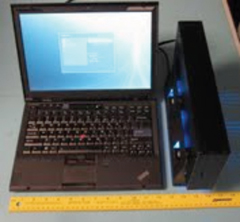
The January 2010 deployment included a WAAS GPS receiver, spectrum analyzer, and a Zeta custom-developed Snapshot System, assembled from commercial off-the-shelf (COTS) equipment for conducting WAAS site-installation surveys, and capable of capturing intermittent short-duration RFI events. It consists of a tuneable receiver (10 MHz to 3 GHz) whose RF front end spans 25 MHz that is digitized at a sample rate of 56 MHz, with storage capacity sufficient for up to 80 minutes. Once captured, the time-series data can be analyzed in many different ways. Possible analysis techniques include examination of the raw time samples, generation of spectral plots, or demodulation of the RFI signal. Each approach can lead to a better understanding of the underlying interference signal. If digital data is present and can be demodulated, it might be possible to associate the demodulated bits with a known transmitter.

Data can be captured manually or programmatically using a trigger determined by an algorithm that monitors WAAS GPS receiver automatic gain control (AGC) logs. The AGC function within a WAAS receiver has a well-behaved response for normal Gaussian noise RF environments. When RFI is present, the AGC exhibits atypical responses that then trigger the Snapshot System. As WAAS receivers utilize both L1 and L2, and each RF path has its own AGC, it is possible to detect the presence of potential RFI at either L1 or L2.

The Snapshot System RF input for this deployment was from a PCTEL antenna identical to those used at WAAS reference sites. This antenna incorporates a triplexer that provides three separate 40 MHz passbands each centered on L1, L2, and L5, with approximately 50 dB of gain. This antenna was located approximately one mile north of the four LAAS antennas within Port Authority of New York and New Jersey (PANYNJ) Building 80.

Within the first hour of being deployed on January 20, 2010 the Snapshot System had detected and captured one RFI event in the GPS L1 band. After one day, the Snapshot System had detected and captured more than 25 separate instances of RFI within the GPS L1 band. Most RFI events were narrowband (10s of kHz bandwidth) and short duration (no more than 3 seconds).

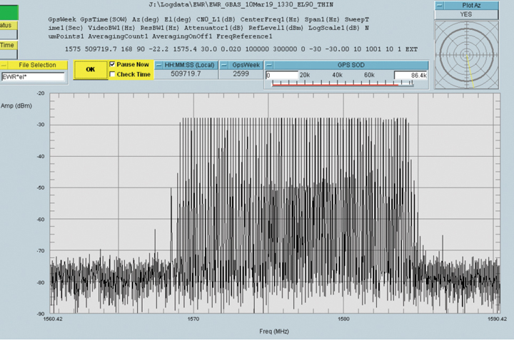
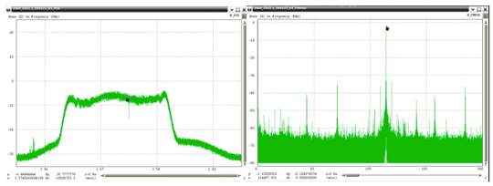
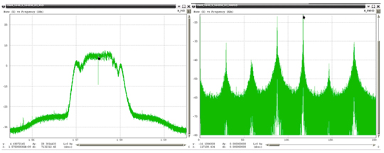
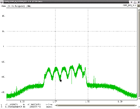
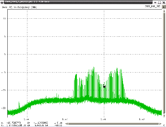
However, there also were five RFI events that spanned more than 15 MHz across L1 (Figure 1) were present as long as 20 seconds and at a power level as much as 25 dB above the receive antenna’s noise floor. Some of these RFI events were strong enough to reduce a WAAS G-II receiver C/N₀ by as much as 20 dB and thereby resulted in loss of tracking for lower-elevation GPS satellites. Higher-elevation GPS satellites were able to continue tracking throughout these events but at a lower C/N₀. The wideband RFI events were also detected by the SLS 4000 GBAS monitor and coincided with tracking problems in the LAAS GBAS receivers.

FIGURE 1. EWR wideband RFI.

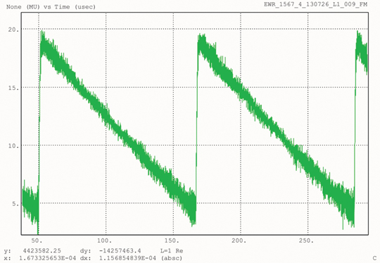
Two of the captured broadband RFI events were demodulated and analyzed. The underlying linear frequency modulation (FM) signal swept over more than 15 MHz in less than 1 millisecond (Figure 2).

FIGURE 2. FM demodulated wideband RFI.

At that time, it was not known if the source of the RFI was stationary or moving, whether it was unintentional (emanating from a licensed transmitter but with malfunctioning electronics), inadvertent (equipment normally used for test purposes and capable of operating in the GPS band but accidentally left on), or intentional (purposeful jamming of GPS).

Since the RFI was observed by GPS receivers separated by 1,700 meters, a search was undertaken to identify any other GPS receivers in the vicinity of EWR. One National Geodetic Survey (NGS) continuously operating reference site (CORS) NJI2 is located near EWR about 4,500 meters northwest from Building 80. Analysis of data from NJI2 during the same time periods that RFI was detected by the WAAS and LAAS receivers did not contain any indication of RFI, and therefore suggested that the source of RFI was more localized to EWR.

The Snapshot System remained in place for approximately two weeks before moving to another location. Collected data was analyzed, showing that wideband RFI was associated with significant degradation to both the WAAS and LAAS receivers. Additional characteristics noted the RFI was intermittent, lasting typically 30 seconds but no more than 60 seconds, was observed more often Monday through Friday, and most frequently around 8 a.m. local time.

Locating The RFI

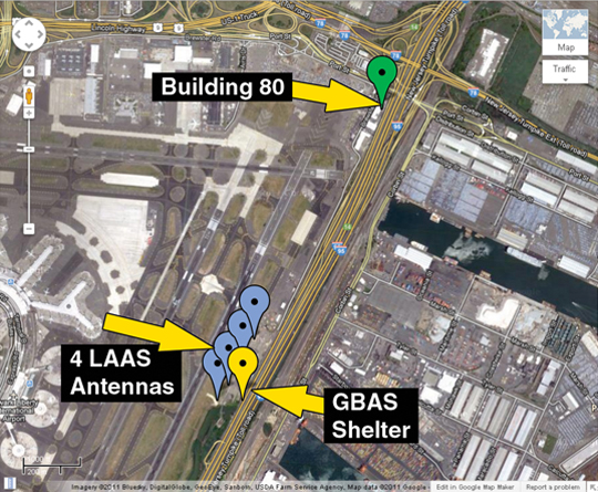
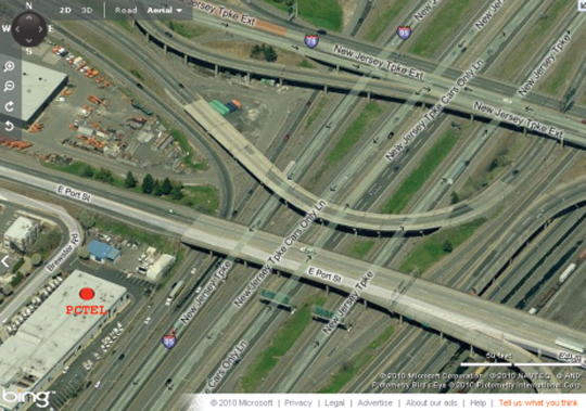
Figure 3 shows a Google map of EWR with blue dots indicating the location of the four LAAS antennas, a green dot for Building 80, and a yellow dot for the GBAS shelter. EWR is adjacent to the New Jersey Turnpike (NJT), which has seven southbound and seven northbound lanes of traffic.

FIGURE 3 Google map of EWR.

Since the Snaphsot System did not include location capability, other teams with direction-finding equipment, including beam-forming antennas, travelled to EWR to try to locate the RFI source. These teams were on site at various times from February to March. However, those efforts did not provide sufficiently reliable information to reduce the search area. By mid-March, the search area remained identical to that of January.

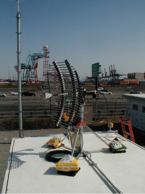
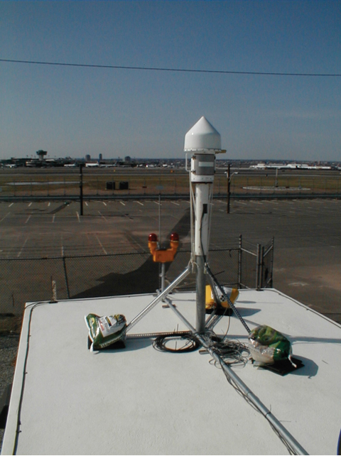
Zeta then deployed two WAAS G-II receivers separated by considerable distance (1,722 meters) to monitor for RFI, and analyze each receiver’s response only when RFI sufficient to significantly degrade GPS reception was detected. One receiver was located within Building 80, and the second receiver within the GBAS shelter near the LAAS antennas. This configuration was designed to determine degradation relative to each reference receiver and thereby establish probable search areas for the RFI emitter. The Zeta equipment also incorporated a rotating directional antenna (at the GBAS shelter shown in Figure 4) that was commanded to rotate only when significant RFI was detected.

FIGURE 4A. Antennas on roof of GBAS shelter.

FIGURE 4B. Antennas on roof of GBAS shelter.

The expectation was that RFI would be detected simultaneously by both GPS receivers, and that the relative degradation in normalized C/ N0 would provide an indication as to which location lay in closer proximity to the RFI source. The rotating high-gain directional antenna would then indicate a reduced probable search area consistent with the relative degradation between the two receivers. At the time this equipment was deployed, it was still thought that the RFI was most likely stationary and high-power. However, the measurement results were quite different than expected. Subsequent data analysis from this equipment revealed that the RFI was low-power and moving, specifically moving along the NJT.

The Zeta equipment was deployed on March 19, 2010, and remained in place while operating automatically. On March 25, data collected during the previous week were analyzed. During this 1-week collection there were 11 instances when both receivers detected wideband RFI events and one antenna rotation even partially tracked one wideband RFI emitter. Such data was indicative of a non-stationary emitter, a finding that was quite significant. Based on data from the two receivers, the apparent velocity of the RFI emitters ranged between 45 miles per hour (mph) to 72 mph. Initial analysis of antenna-rotation data also indicated the RFI source was east of the GBAS shelter and moving south on the NJT.

Understanding the importance of degradations from both receivers was crucial in determining that the RFI has attributes of transmitting at low power and is moving. Had a single stationary RFI emitter been responsible for these observations, the degradations measured at each receiver would have occurred at essentially the same time, not 50 to 80 seconds apart. A high-power moving RFI emitter would also have produced degradations at both receivers at the same time, and since that was not observed, the conclusion was that the RFI emitter was relatively low in output power. Low-power RFI emitters will cause significant degradation to GPS receivers only when they are in close proximity to them, on the order of hundreds of meters.

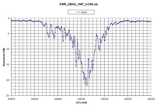
Receiver data logs were processed specifically for degradation in normalized C/N₀. Normalized C/N₀ was only computed for those satellites above 20 degrees, and all of those results were averaged together. Prior knowledge regarding WAAS PCTEL antennas has established an expected C/N₀ versus satellite elevation that is accurate to approximately ±1 dB with a nominal mean of 0 dB. This normalized C/N₀ represents an average of all satellites in view. However, individual satellite signal strength can vary greater than ± 1 dB. Significant deviations of more than –3 dB are indicative of strong RFI within the GPS processing band. Normalized C/N₀ was plotted for each day that data was collected, followed by expanding those time periods where significant degradation was present.

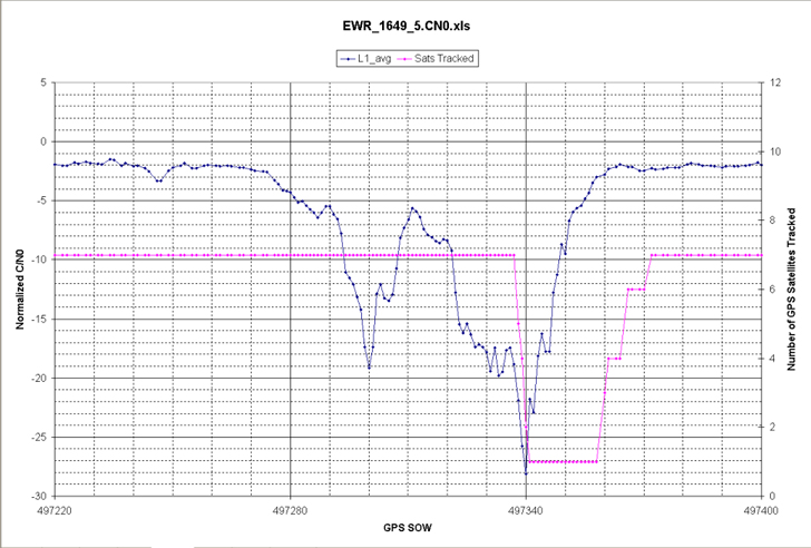
Figure 5 shows data of the first evidence of a low-power moving PPD. Data for Building 80 receiver is in blue and data from the GBAS shelter receiver in pink. Since Building 80 is north of the GBAS shelter, when degradations occurred first at Building 80, this implies that the RFI emitter is moving from north to south. Similarly, when degradations were first seen at the GBAS shelter, the RFI emitter was moving from south to north. This plot uses major time grids of 60 seconds and minor grids of 10 seconds.

FIGURE 5. Normalized C/N0 observed at Building 80 and GBAS shelter.

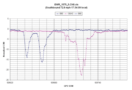
The double separate degradations observed by the Building 80 receiver have only been observed from monitoring equipment located at that building, and have since been associated with travel paths of PPDs on the nearby highways. Both GPS receiver and spectral data contain this same characteristic. This characteristic is due to the fact that vehicles traveling south on the NJT have clear line of sight to the roof of Building 80 (shown by Figure 6) before they travel under Interstate 78, after which they pass next to Building 80. During the time that they are under Interstate 78, their transmissions are blocked in the direction of the roof of Building 80.

FIGURE 6A. View of NJT near Building 80.

FIGURE 6B. View of NJT near Building 80.

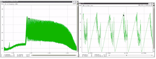
Spectral data as observed by the 4-foot reflector is shown in Figure 7. Figure 8 shows spectral maximum data as collected by the 4-foot linearly polarized reflector along with additional information.

FIGURE 7. Wideband RFI observed by 4-foot reflector (click to enlarge.)

FIGURE 8A. Pink represents spectral maximum data as observed through the reflector, green represents the azimuth of that antenna, and blue the reported degradation of the GBAS shelter receiver.

FIGURE 8B. Pink represents spectral maximum data as observed through the reflector, green represents the azimuth of that antenna, and blue the reported degradation of the GBAS shelter receiver.

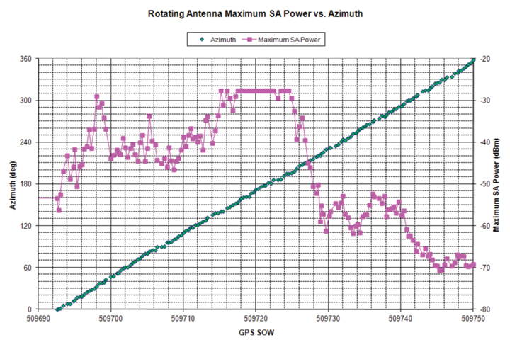
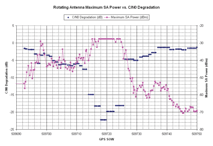
When the GBAS shelter receiver at first detected RFI, the reflector began rotating from an azimuth of 0 degrees in a clockwise direction. At the same time, a spectrum analyzer began capturing spectra at a rate of 3 per second. The first spectral maximum was observed at an azimuth of 30 degrees, a direction in which the antenna was pointed towards the NJT, to a location approximately 900 meters away from the GBAS shelter. The next time spectra were at high levels occurred for azimuths between 145 to 195 degrees, or southeast of the GBAS shelter. The approach of using a rotating antenna was originally intended to provide a direction towards a stationary source and not to track a moving emitter. However, it appears that to some extent, the rotating antenna in fact did track a moving emitter from north to south.

On the afternoon of the day these results were communicated to the FAA lead for the EWR RFI investigation, all search activities were shifted to the NJT and away from the airport operating area. Just south of the GBAS shelter there is an official-use overpass that straddles the NJT. All detection equipment was positioned onto the overpass, under the hypothesis that the RFI was emanating from vehicles traveling the NJT. Evidence substantiating this initial finding was found within a day, and approximately one month later a concerted effort was undertaken to identify and stop a single vehicle that was using a PPD.

The Zeta equipment remained in place for many months and continued to provide additional evidence of PPD characteristics. Early in the investigation it was hoped that only a few PPDs had been responsible, but as more data was collected it became evident that many different types of PPDs were traveling along the NJT past EWR.

Modeling PPD Effect

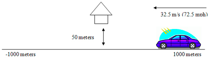
Once it was realized that the RFI was from low power moving emitters, a simple model was used to predict their degradation effect on WAAS GPS receivers. The model shown in Figure 9 was used for the purpose of computing distance between the RFI emitter and a WAAS antenna and to then compute the additional level of interference noise power that the WAAS antenna would receive. Here, the WAAS PCTEL antenna is located 50 meters from a road that is 2000 meters long and straight and has an RFI emitter transmitting +25 dBm, moving at 32.5 meters per second (72.5 mph) and with clear line of sight to the WAAS antenna.

FIGURE 9. Simple model of moving emitter.

FIGURE 10. Model of normalized C/No due to a PPD.

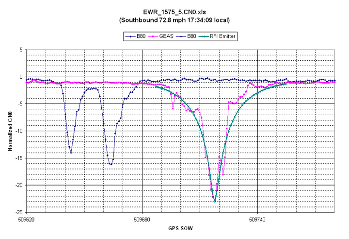
With these assumptions it is a simple matter to compute the additional noise power at the WAAS antenna. Non-coherent summation of the RFI noise and inherent system noise was used to compute the total noise power and therefore the additional degradation in C/N₀. The resulting predicted degradation was overlaid on one of the actual RFI events and is shown as a green line in Figure 10. The predicted degradation closely resembles actual event data logged by receivers.

The shape of degradation in normalized C/N₀ versus time has been observed in nearly all of the EWR RFI events that have been analyzed. The magnitude of degradation depends on the power of the RFI and its proximity to the GPS antenna, while its time duration depends on the velocity of the vehicle carrying the PPD. The shape is directly related to the distance versus time between the vehicle and the WAAS antenna. Faster/slower moving vehicles with PPDs will simply shrink/stretch the time scale. Curved roadways would have different shapes that could also be readily predicted.

CORS data was revisited after realizing that PPDs were traveling the NJT. Specifically, two CORS sites CTDA (70 meters from Interstate 95) and NJDY (380 meters from Interstate 95) were identified. Data from those two sites were analyzed for a couple of weekdays. Possible evidence of PPDs was found within that data. Reported Signal to Noise Ratio (SNR) from CTDA and NJDY contained variations similar to those observed by GPS receivers at EWR during times when PPD induced RFI has been detected.

Continued RFI Monitoring

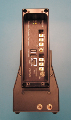
The LAAS program desired continued monitoring of RFI from PPDs near EWR, including estimates of their effective isotropic radiated power (EIRP). Additional equipment was assembled to provide this capability and installed on March 3, 2011. This monitoring equipment is located within the GBAS shelter at EWR and comprises several COTS components that incorporate improvements beyond the first Snapshot System used at EWR. Improvements include an upgraded Snapshot System (Figure 11), an RHCP directional antenna, and a wireless modem that provides remote access to the monitoring equipment.

Figure 11A. Snapshot System ICEPOD6-M5.

FIGURE 11B. Snapshot System laptop.

Remote access makes it possible to analyze captured RFI data from any computer connected to the Internet, and to modify software if necessary. The new equipment configuration, specifically the use of an AEL AST 1507AA RHCP antenna, was chosen with the explicit purpose of establishing more accuracy in estimated EIRP.

Analysis of data collected during 2010 indicated three significant sources of error in estimating EIRP; Free Space Loss (FSL) from not knowing the exact position of the PPD on the NJT, polarization mismatch loss between the PPD antenna and the receive antenna, and the effects due to transmission from within a vehicle. Differences in FSL loss between the closest southbound lane on the NJT and the most distant northbound lane is on the order of 11 dB. If it is known that the PPD is traveling south, the difference in FSL between the nearest to farthest southbound lanes is less but still about 6 dB. FSL differences for northbound lanes are smaller, on the order of 3 dB. Knowing the direction of travel reduces this uncertainty but does not eliminate it. The WAAS PCTEL antenna is RHCP, but at the horizon has an axial ratio of approximately 5 dB. Many PPDs appear to be using quarter wavelength dipole antenna that are mounted with a rotatable connector. Assuming all PPD antennas are linearly polarized, there would then be an uncertainty of about 5 dB when using data observed by the WAAS PCTEL antenna. The AEL antenna has an axial ratio of 0.2 dB at L1 and significantly reduces uncertainty of polarization mismatch loss. Even though the AEL antenna has a 3 dB mismatch loss, that loss has an uncertainty of 0.2 dB for any orientation of the PPD antenna. The PCTEL antenna has a symmetric gain response relative to the NJT. The AEL antenna was pointed to the north intentionally so that observed RFI power will be stronger when a PPD is north of the GBAS shelter. Simultaneous capture of real time samples from both antennas by the ICEPOD6-M5 provides an indication of the direction in which the PPD is traveling. The third uncertainty comes from the effects of the PPD being located within a vehicle. Vehicular effects on the PPD transmitters were not accounted for due to difficulty in using a simple model. Aloi [1] has measured vehicular effects of quarter wavelength dipole antenna (typically used by PPDs) and has previously published [1] [2] on the effect of vehicles on GPS signals. His most recent findings have not yet been published but indicate that the type of vehicle, the location of a dipole antenna within it, and the position outside of the vehicle from which power is being measured, can lead to significant variation (10 to 15 dB) of the observable power. Consequently, the reported EIRP estimates from the Snapshot System have been referenced to a point just outside the vehicle and do not attempt to account for vehicular effects.

Figure 12 shows a block diagram of the current monitoring equipment. The PCTEL antenna along with the WAAS G-II receiver is used for monitoring GPS signals. WAAS G-II receiver logs are monitored continuously and saved to disk, but snapshots are only taken if the RFI algorithms indicate that RFI is present. A snapshot will be taken if any of three tests (based on AGC, normalized C/N₀, or spectral power) are exceeded. Narrowband RFI tends to most impact the AGC response, while wideband RFI tends to trigger the normalized C/N₀ metric. Since the Snapshot System is also continuously monitoring the RF spectra from both antennas, an additional test checks if there are significant spectra changes.

FIGURE 12. Current Snapshot monitoring block diagram.

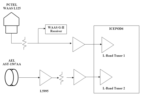
The AEL antenna is connected to a filter/low noise amplifier (LNA) (Delta Microwave L5995) identical to those within the PCTEL antenna, before it is connected to one of the two L-band tuners (900 to 2200 MHz) of the ICE-Online ICEPOD6-M5, which includes 1 TB of long-term storage and 8 GB of high-speed RAM and is capable of sustained data transfers of as high as 400 MB/s between the L-band tuners and disk. Sample rates and RF filtering are programmable and have been set to use a complex sample rate of 40 MSPS and an RF bandwidth of 30 MHz. When RFI is present, data transfers are 320 MB/s. The internal 1 TB disk can store approximately 100 minutes of RFI. Software parameters limit RFI data capture for any single event to no more than 90 seconds. Implementation of a circular buffer within the high-speed RAM (8 seconds for each L-band tuner path) allows continuous capture of RF data while waiting for a trigger indicating that RFI is present. To reduce false alarms, RFI must be present for at least 4 seconds before data is captured. However, no RFI data is lost, because the circular buffer is longer than 4 seconds. RFI data captures typically contain 3 seconds of data at the beginning, with no RFI, and therefore make it possible to observe the onset of the RFI.

The new equipment has captured hundreds of RFI events, spanning a wide range in bandwidth (7 MHz to an estimated 150 MHz), chirp rate (9 kHz to 170 kHz), and power levels (–10 dBm to as much as +20 dBm). Accurately estimating EIRP of moving emitters is a challenge and requires detailed knowledge of the characteristics of all components used in generating the estimate. Furthermore, distance to the RFI source can only be inferred, since its movement precludes exact measurement, and consequently there will always be some uncertainty in any reported EIRP. However, even with these qualifications, there is evidence from Snapshot System data that some of the RFI sources are transmitting at power levels as much as +20 dBm.

Modeling Antenna Responses

The use and orientation of the two antennas was chosen to determine the direction that PPDs are traveling and thereby reduce some of the uncertainty with respect to their exact location. Figure 13 shows the direction (58 degrees) in which the AEL antenna is pointed.

FIGURE 13. Pointing direction of the AEL antenna.

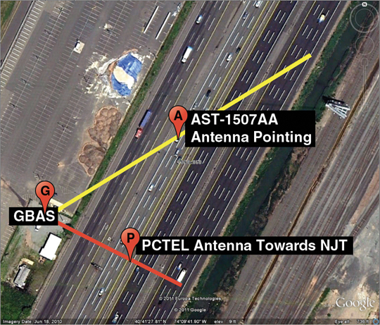
The combination of its beam width (70 degrees) and axial ratio (0.2 dB) results in a nearly uniform gain across all lanes north of the GBAS shelter. Although FSL still depends on the exact location of the PPD, this approach does reduce many of the uncertainties associated with estimating EIRP. Since the PCTEL antenna has an omnidirectional pattern it will have a symmetrical response.

To determine the time that maximum PPD power would be observed by each antenna, a model was used that assumed the PPD was transmitting at constant power, with fixed polarization, travelling at a constant velocity, and there were no obstacles between the transmitter and each antenna. FSL was calculated for each second of travel and used to determine the magnitude of RFI power that would be received. This value was then used to calculate a nominal Interference to Signal (I/S) relative to the GPS signal. The distance between each antenna and each of the travel lanes on the NJT were also used. The intent of this model was to understand how I/S would vary with time for each of the NJT travel lanes. Figure 14 shows the predicted I/S for the PCTEL antenna and Figure 15 for the AEL antenna. In each of these plots red, yellow and orange represent 3 of the 7 south bound travel lanes and green, blue and purple represent 3 of the 7 north bound travel lanes. A time of 0 was used for the time when the PPD is nearest physically to the GBAS shelter. A nominal velocity of 30 meters/second (67 MPH) was used for the PPD and I/S was computed for 30 seconds before and after its closest approach (± 900 meters north and south of the GBAS shelter). If the PPD travels slower than 30 m/s then the following curves would be wider for the same times. Similarly, if the PPD travels faster, these same curves would be narrower.

FIGURE 14. Predicted I/S for PCTEL antenna (click to enlarge.)

FIGURE 15. Predicted I/S for AEL AST-1507AA (click to enlarge.)

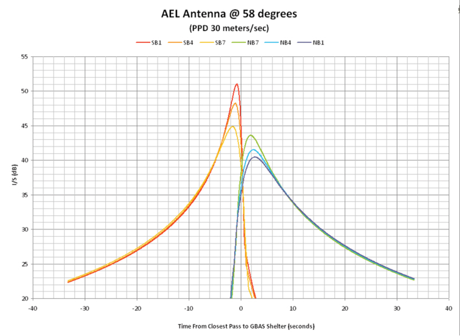
Modeling of the AEL antenna took into account its pattern and orientation. It has less gain towards the south, and consequently observed power from a PPD located south of the GBAS shelter is much less. A southbound PPD will initially be within the main beam of the AEL antenna; therefore the expected interference to signal ratio (I/S) will gradually increase until it passes to the south of the GBAS shelter. Similarly, a northbound PPD will not exhibit significant I/S until north of the GBAS shelter. Figure 15 indicates that the maximum I/S occurs within 2 seconds of the point where the PPD is closest to the GBAS shelter. Typical GPS receivers can tolerate an I/S of 30 dB for CW type signals.

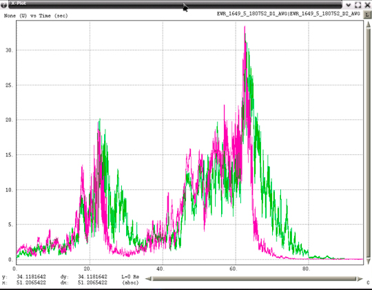
Processed RFI data does display some of these characteristics but with some important differences. PPD power was measured once every millisecond using Snapshot System data and total power within the bandwidth of that PPD was calculated. Total power from both the PCTEL (green) and AEL (pink) antennas were then plotted together with one example for a southbound PPD in Figure 16 and a northbound PPD in Figure 17.

FIGURE 16. RFI Power of southbound PPD (click to enlarge.)

FIGURE 17. RFI Power of northbound PPD (click to enlarge.)

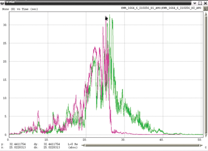
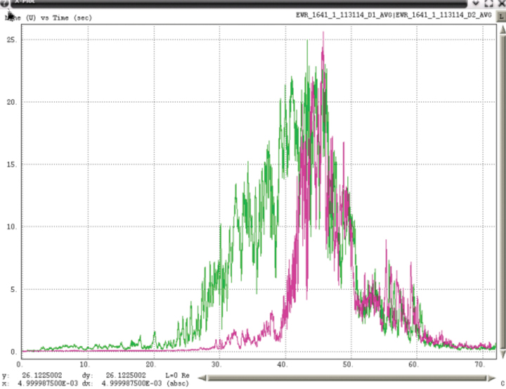
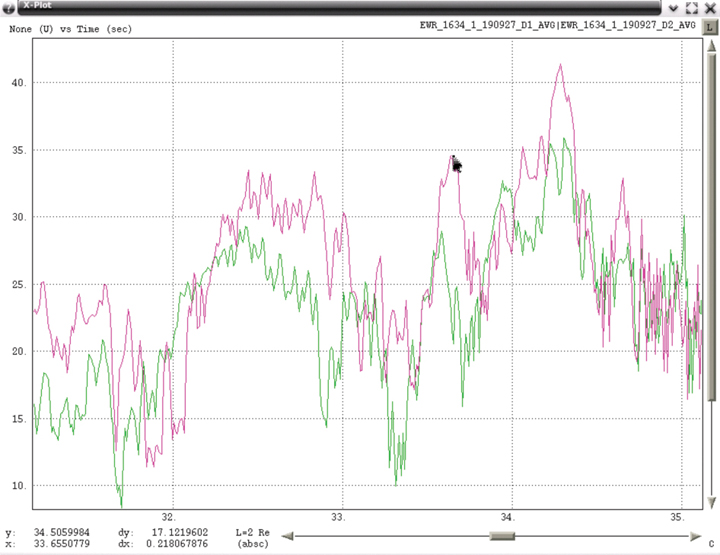
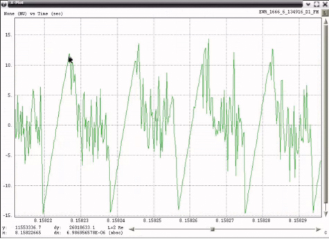
Although the envelope of the measured average power tends to have the shape that modeling predicts, there are significant variations over short periods of time. Figure 18 expands a portion of one example and indicates that RFI power varied by more than 17 dB in 0.2 seconds. Examination of spectral data for time intervals of less than one second frequently contains significant changes in observable power. Swept CW from PPDs should exhibit relatively flat RF spectral power, but typical observed spectra include sloping across the band and notches. Possible explanations for these observations include: blockage and diffraction from other vehicles near the one containing the PPD, multipath from other vehicles on the NJT, and the effect of transmitting from within a vehicle. Although some of the snapshot captures exhibit smooth power variation similar to predicted, the vast majority of the hundreds of snapshots exhibit significant variations in power.

FIGURE 18. RFI Power of southbound PPD (expanded).

Examples of Observed PPDs

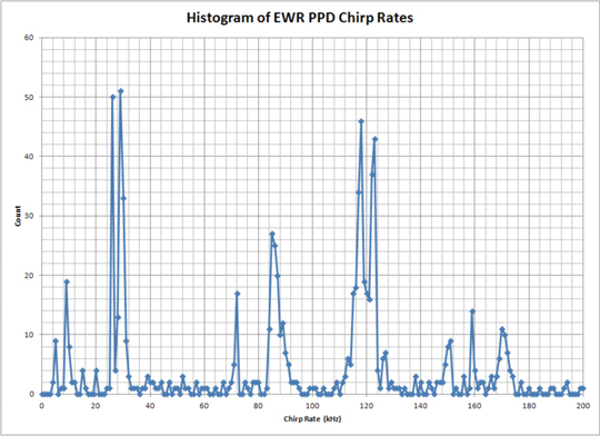
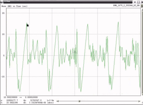
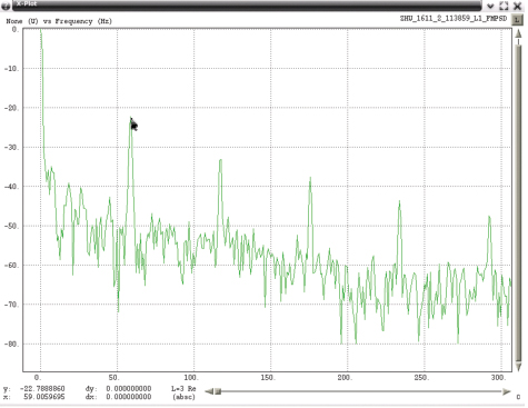
The variety of PPDs observed by the updated EWR monitoring equipment has been surprising. Within its first month of operation, more than 40 PPDs were observed with no less than 19 from unique and different PPD transmitters. Classification of PPD transmitters is based on the combination of RF spectra and the spectrum of the FM demodulated data. Although the observed PPD transmitters use a linearly swept FM sawtooth, most contain deviations from a pure linear sweep. Figure 19 shows examples of FM demodulated time series. Rather than attempting to uniquely describe the attributes of each type of deviation, it is simpler to compute the spectrum of the FM demodulated data. The fundamental frequencies of chirp rates that have been observed have spanned 9 kHz to 170 kHz. Figure 20 shows a histogram of chirp rates observed near EWR and indicates that the most frequent rates have been 9, 26, 29, 72, 85, 118, 123, 159 and 170 kHz.

FIGURE 20. Histogram of EWR PPD chirp rates.

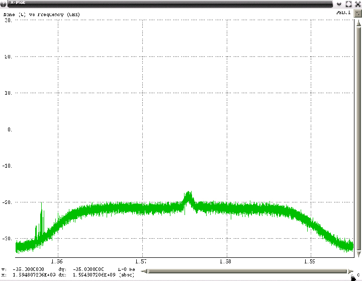
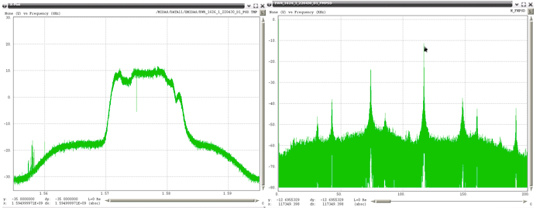
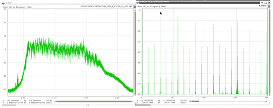
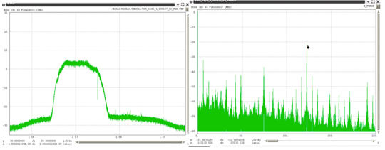
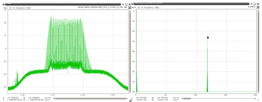
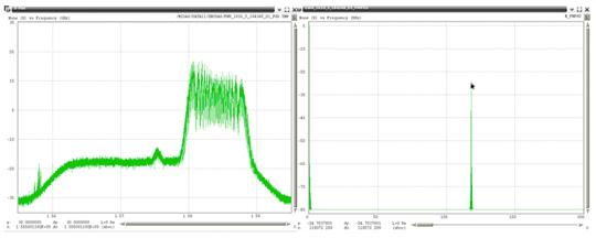
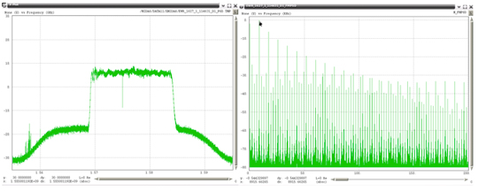
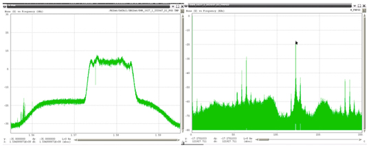
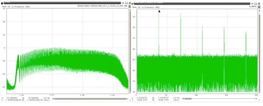
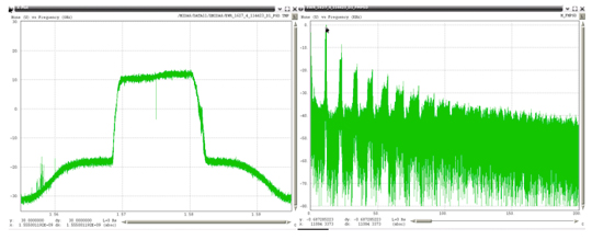
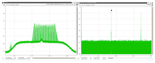
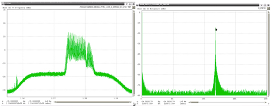
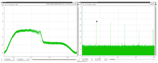
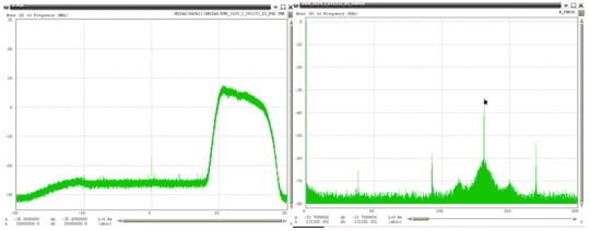
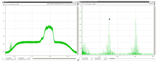
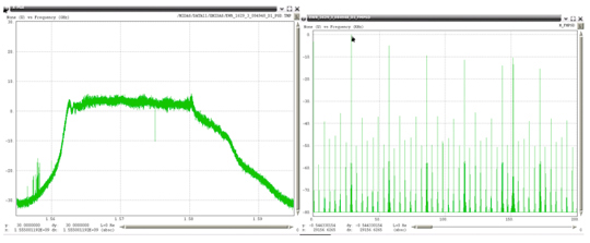
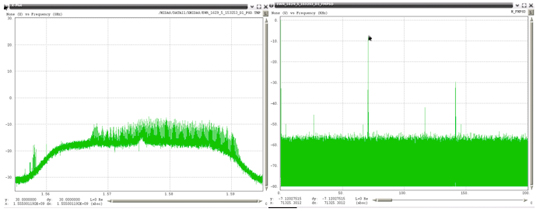
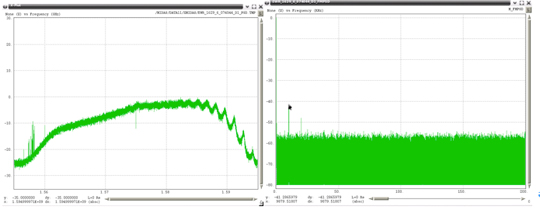
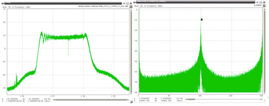
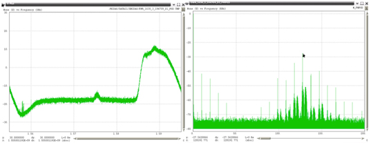
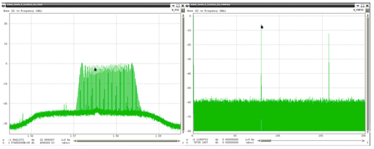
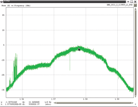
Examples of the 19 unique PPDs (detected within one month) are shown in Figure 22 through Figure 40, with the RF spectrum shown on the left, and the spectrum of the FM demodulated shown on the right. In each of these plots the scaling for the RF spectra is identical, spanning 40 MHz centered on 1575 MHz with a vertical scale using 10 dB per grid. All of the FM demodulated spectra use a horizontal axis that spans 0 to 200 kHz. For references purposes Figure 21 shows the RF spectra when no RFI is present.

Some of these PPDs were transmitting at power levels (observed by the PCTEL antenna) as much as 40 dB above the LNA noise floor. Most spectra were not centered symmetrically about L1 with some completely outside the mainlobe of the GPS C/A code. A few were transmitting outside the programmed 40 MHz bandwidth of the Snapshot System (1555 to 1595 MHz). For those PPDs transmitting outside this band, estimates were made of the upper or lower frequencies using the linear slope of the FM demodulated data, and then extrapolating that slope based on the chirp interval.

Some of the FM demodulated spectra contain a single spectral line that indicates the waveform modulating the RF has a very linear sweep. Most contain additional harmonic lines about the major component and a few appear to have bandwidth about their main spectral component. The current hypothesis is that many of these devices are poorly shielded and that the internal oscillator used to modulate the RF is affected by other nearby signals that are then appearing at the RF output. Some of the possible sources could be circuits that are within the device itself but there is some evidence that a few of these devices are susceptible to energy external to the PPD. A Snapshot System located near Houston International Airport (ZHU) has captured data from PPDs that contain strong components at 58.7 Hz in addition to its linearly swept 97 kHz waveform. Since this frequency is sufficiently different from utility AC power sources (60 ± 0.03 Hz), it has been hypothesized the vehicle carrying that PPD, also has a power inverter. Most power inverters are specified to provide a frequency output of 60 ± 3 Hz. Figure 32 shows a spectral notch that was present at that single frequency throughout the complete capture and suggests that that particular device may have had an impedance matching problem in its transmission path.

FIGURE 21. Spectra with No RFI Observed by PCTEL (click to enlarge).

FIGURE 22. 1570 to 1583 MHz, Chirp 117.35 kHz.

FIGURE 23. 1556 to 1583 MHz, Chirp 28.43 kHz.

FIGURE 24. 1565 to 1578 MHz, Chirp 123.13 kHz.

FIGURE 25. 1568 to 1583 MHz, Chirp 111.08 kHz.

FIGURE 26. 1578 to 1589 MHz, Chirp 118.07 kHz.

FIGURE 27. 1568 to 1584 MHz, Chirp 8.92 kHz.

FIGURE 28. 1572 to 1584 MHz, Chirp 121.93 kHz.

FIGURE 29. 1557 to 1622 MHz, Chirp 36.14 kHz.

FIGURE 30. 1568 to 1582 MHz, Chirp 11.08 kHz.

FIGURE 31. 1570 to 1585 MHz, Chirp 85.06 kHz.

FIGURE 32. 1572 to 1582 MHz, Chirp 118.07 kHz.

FIGURE 33. 1529 to 1577 MHz, Chirp 39.52 kHz.

FIGURE 34. 1578 to 1594 MHz, Chirp 131.33 kHz.

FIGURE 35. 1575 to 1582 MHz, Chirp 75.66 kHz.

FIGURE 36. 1561 to 1586 MHz, Chirp 29.16 kHz.

FIGURE 37. 1568 to 1592 MHz, Chirp 71.33 kHz.

FIGURE 38. 1560 to 1595 MHz, Chirp 9.88 kHz.

FIGURE 39. 1564 to 1582 MHz, Chirp 100.48 kHz.

FIGURE 40. 1584 to 1599 MHz, Chirp 128.20 kHz.

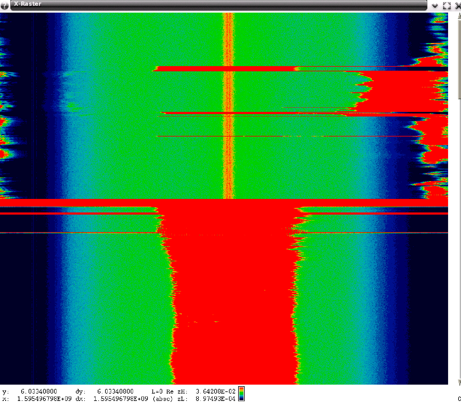
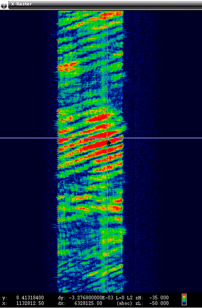
A few snapshots have also provided evidence that some of the PPDs are erratic and probably not functioning as their manufacturer intended. Figure 41 contains a raster of 6 seconds of spectral data that shows a PPD whose output was meant to be between 1560 and 1580 MHz but for short periods of time was transmitting at frequencies above 1580.

FIGURE 41. Spectral Raster, PPD with Unstable Output.

Remarks on Additional PPDs

Since April 2011 the Snapshot System has captured many additional and different PPDs. No effort has been carried out to catalog all of the different types that have been observed but the following describes interesting and notable PPDs.

Figure 42 shows characteristics of a PPD that has had estimated EIRP approaching +20 dBm, to a point just outside the vehicle, and has also been associated with GPS receiver C/N₀ degradation of more than -27 dB, strong enough to cause the WAAS receiver, located at the GBAS shelter, to lose lock on all GPS satellites for a short period of time.

FIGURE 42. 1568 to 1582 MHz, Chirp 118 kHz

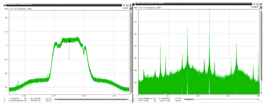
Figure 43 shows a PPD that is one of the most frequently observed PPDs but that has not been associated with any significant degradation to the GPS receivers. Estimated EIRP for these PPDs has been on the order of no more than +10 dBm. One device with similar characteristics was procured and its measured power at the antenna output port was no more than +14 dBm. Marketing information on the internet for that PPD specified its output power as +25 dBm.

FIGURE 43. 1572 to 1589 MHz, Chirp 85 kHz.

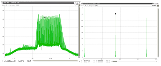
Figure 44 shows a PPD that is transmitting at both L1 and L2. The EWR Snapshot System has been configured to only capture snapshot data at L1 due to the fact that LAAS only uses L1. However, the WAAS receiver used to monitor for RFI is a dual frequency receiver that on occasion has indicated simultaneous RFI at both L1 and L2. Even though the EWR Snapshot System has not captured data at L2, the simultaneous presence of both L1 and L2 RFI, provides strong circumstantial evidence that this RFI source was transmitting on both frequencies. A Snapshot System monitoring the WAAS Reference Station (WRS) at Leesburg Virginia has captured simultaneous L1 and L2 RFI events. Demodulation of that data indicated the two RF outputs had similar modulation but the demodulated data was not coherent. Therefore, that PPD was probably using individual, but similar waveform generators, for each RF output.

FIGURE 44. 1562 to 1583 MHz, Chirp 114 kHz.

Almost all PPDs have been observed individually. However, there have been at least three times in the last two years when two unique PPDs have been observed within 60 seconds of each other. Figure 45 plots normalized degradation in C/N₀ while Figure 46 plots snapshot measured power for the same RFI event. Analysis of snapshot data for each of the times that had strong RFI power are shown in Figure 47 and Figure 48 and confirmed that there were in fact two unique PPDs observed approximately 40 seconds apart. Both were traveling south on the NJT and approximately 1200 meters apart.

FIGURE 45. Normalized C/N0 August 19, 2011

FIGURE 46. Snapshot Power August 19, 2011.

FIGURE 47. C/N0 -19.0 dB, Chirp Rate 78.97 kHz.

FIGURE 48. C/No -28.0 dB, Chirp Rate 117.24 kHz.

Most of the observed RFI events last for no more than 50 seconds although a few that lasted much longer have been correlated with slow traffic on the NJT. Figure 49 is from June of 2010, before the updated monitoring equipment was in place, and displays normalized degradation of C/N₀. The time duration for which this RFI was observed was more than 3 minutes and was during a time when traffic was ‘slow’ on the NJT.

FIGURE 49. June 9, 2010, PPD, Estimated Velocity 10 m/s.

Very wide-bandwidth PPDs have recently been observed more often. The frequency span these devices are transmitting has had to be estimated due to the fact that the Snapshot monitor has 40 MHz of bandwidth, and these PPDs are transmitting beyond this bandwidth. Figure 50 through Figure 52 show examples of these types of PPDs. The left plot in these figures is the RF spectra and the right plot is the FM demodulated waveform. The latter each contain a linear component that is present for only a portion of the chirp interval. Under the assumption that the modulating waveform would be linear for the repetition interval, the slope of the visible linear component was extrapolated to the total chirp time interval. It is not possible to estimate the upper and lower frequency points for the last two examples, since neither of those had a frequency that began or ended within the observable 40 MHz bandwidth of the monitor.

FIGURE 50. 1566 MHz to 1601 MHz, chirp 26.74 kHz.

FIGURE 51A. Estimate 70 MHz span, chirp 53.89 kHz.

FIGURE 51B. Estimate 70 MHz span, chirp 53.89 kHz.

FIGURE 52A. Estimate 135 MHz span, chirp 74.69 kHz.

FIGURE 52B. Estimate 135 MHz span, chirp 74.69 kHz.

Although the Snapshot System L-band tuners can be programmed for greater bandwidth, the limiting bandwidth is the bandpass filters contained within the LNA modules, which have bandwidths of 40 MHz.

Data captured by a Snapshot System operating near ZHU contains evidence that external energy may have coupled into that PPD and affected the modulation waveform. Figure 53 shows a plot of the RF spectra and an expanded portion of the FM demodulated spectra indicating the presence of a 58.7 Hz component. A raster of the demodulated FM, shown in Figure 54, highlights the 58.7 Hertz component.

FIGURE 53A. ZHU chirp 118 kHz with 58.7 Hz.

FIGURE 53B. ZHU chirp 118 kHz with 58.7 Hz.

FIGURE 54. ZHU raster of FM showing 58.7 Hz (Click to enlarge).

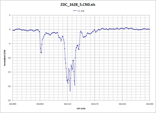
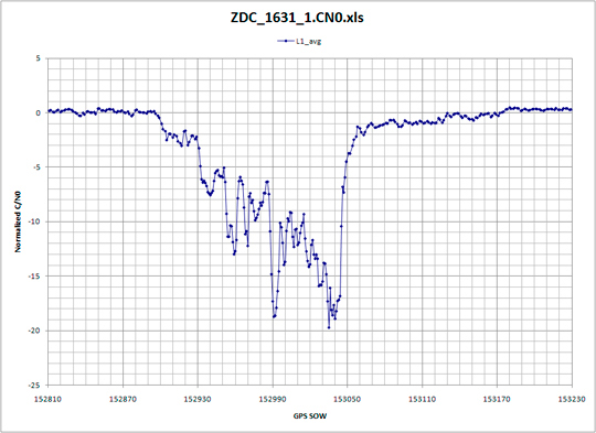
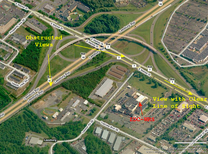
Careful analysis of normalized C/N₀ has also provided clues as to the possible travel paths that a PPD might be using. RFI was suspected at the WRS located at Leesburg Virginia (ZDC). A Snapshot System was installed to detect and characterize possible RFI. Analysis of snapshot data did confirm that a few PPDs were traveling past ZDC. One of the PPDs was more disruptive than the others but fortunately was also following a very predictable schedule. It was regularly detected twice a day, first within 10 minutes of 4:30 AM local and next within 30 minutes of 2:30 PM. Normalized C/N₀ contained similar patterns for each time of day and are shown in Figure 55 and Figure 56. Examination of the local roadways, shown in Figure 57, suggested the possible roads and direction in which this PPD was traveling. The WAAS antennas on the roof of ZDC have clear line of sight to state highway 7 for vehicles that are east of ZDC. Normalized C/N₀ for morning events tended to have a relatively abrupt onset followed by a gradual return to normal while the afternoon events exhibited a gradual increase in degraded C/N₀followed by a quick return to normal. This observation lead to hypothesizing that the PPD was traveling east in the morning and west in the afternoon.

FIGURE 55. ZDC Typical Morning Degradation.

FIGURE 56. ZDC Typical Afternoon Degradation.

FIGURE 57. Roads near ZDC (click to enlarge.)

FAA Spectrum personnel were informed of this analysis and confirmed that this hypothesis was correct. Using this information they were able to detect the vehicle that was responsible and remove this particular PPD from service.

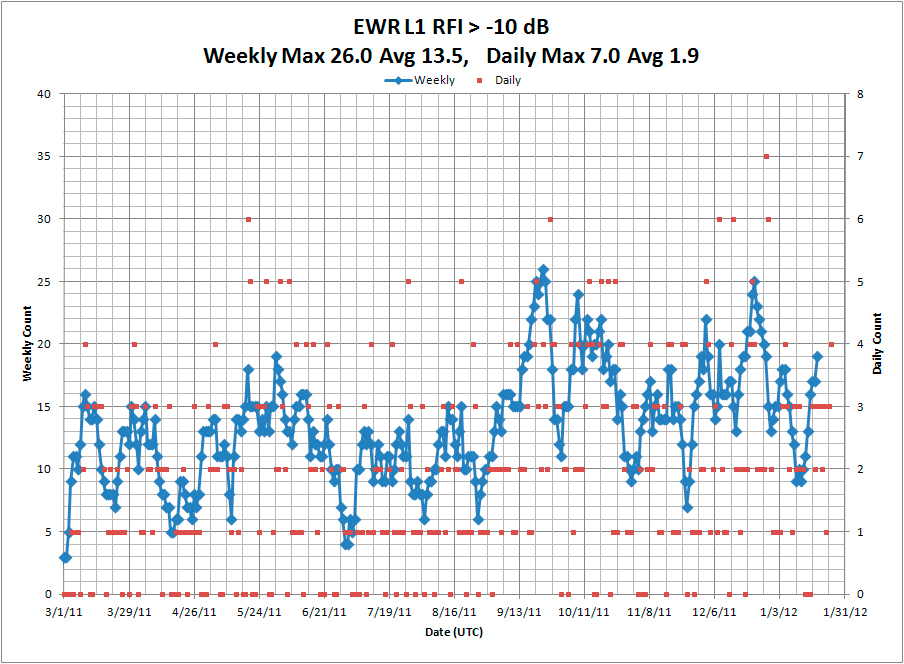
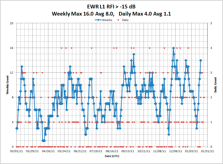
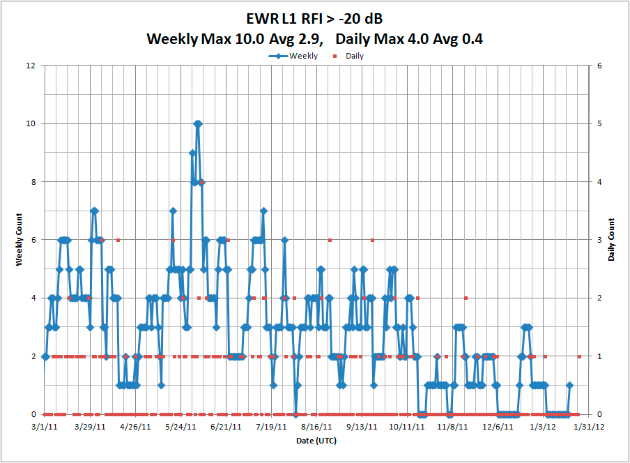
EWR RFI Event Statistics

A large number of RFI events have been detected at EWR since the updated Snapshot System was installed on March 3, 2011. These RFI events have been ranked according to the magnitude of degradation in normalized C/N₀, as reported by the GBAS shelter WAAS receiver. The following plots show the total number of RFI events per day (red dots) and for every seven consecutive days (blue line). On average, PPD-induced receiver degradation of at least 10 dB has been observed two times a day. Although a small number of narrowband RFI events produced receiver degradation of as much as 10 dB, the vast majority of RFI events causing 10 dB or more of receiver degradation are due to PPDs.

Figure 58 indicates that since March 2011, more PPD RFI events are being observed. However, Figure 60 indicates that the higher-power PPDs are not being observed as often. One possible explanation is that the previously observed PPDs have stopped working, and the individuals using them have either not acquired replacements or they have acquired different ones with less-damaging RFI.

FIGURE 58. History of RFI > –10 dB (click to enlarge).

FIGURE 59. History of RFI > –15 dB (click to enlarge).

FIGURE 60. History of RFI > –20 dB.

Many recent PPDs have been transmitting with estimated frequency spans of 65 MHz to 140 MHz. Although the estimated EIRP of many of these very wide bandwidth PPDs has been as much as +10 dBm, their effect on GPS receiver processing has not been as damaging due to the fact that the RFI is within the GPS receiver processing bandwidth for only a portion of the time.

Spectra of Swept FM with Multipath

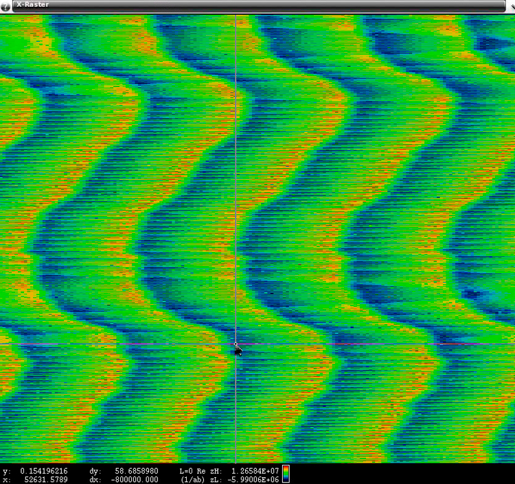
One of the most commonly observed characteristics in PPD spectral data has been uniformly spaced nulls as shown in Figure 61 and Figure 62. Figure 63 displays a spectral raster that shows how the nulls shift in frequency over time. Initially, there was uncertainty as to the mechanism responsible for these observations. Under the hypothesis that multipath might be responsible, a single ray multipath model was used to predict the spectral characteristics of a PPD that includes a multipath component. This analysis was pursued in the hope that it might provide additional information as to the exact location of PPDs.

FIGURE 61. PPD spectral nulls 2.4 MHz apart.

FIGURE 62. PPD spectra nulls 4.7 MHz apart.

FIGURE 63. Spectra raster shifting nulls.

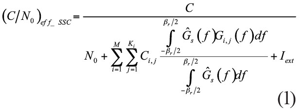
The swept CW signals used by PPDs provide a useful source for characterizing multipath between the PPD and monitoring antennas. Equation (1) models observed CW that is the sum of the direct path and a single reflection in which reflected component has a path length difference of d meters.

(1)

Assuming the reflection is from a metal surface, it should experience a phase reversal. Therefore, destructive cancellation between the direct and multipath component will be present for those frequencies that have a path length difference that is an integer multiple of the wavelength. Equation (2) represents this condition.

(2)

Simplification results in the following expression.

(3)

As an example, if spectral nulls are observed at intervals of 10 MHz, then the path length difference is approximately 30 meters. Spectral nulls have been observed at frequency intervals ranging from 2 MHz to as much as 30 MHz. These null spacing’s translate to path length differences of between 150 meters to 10 meters. Multipath with a path length difference of less than 8 meters will exhibit a single null in the 40 MHz bandwidth of the Snapshot System and therefore cannot be estimated accurately using this technique. A path length difference of 8 meters is also what might be expected for two vehicles traveling side by side on interstate highways since interstate highway specifications require lanes to be approximately 4 meters wide.

Once a possible mechanism for the spectral nulls was hypothesized, additional analysis was performed on specific RFI events in which uniformly spaced spectral had been observed. Snapshot and GPS receiver data indicates the direction of travel for a PPD. With direction of travel known, it is possible to approximate the distance that the PPD is from the monitoring equipment. However, for those RFI events that were examined, the calculated path length difference was similar to or greater than the distance between the PPD and monitoring equipment. The most likely location of surfaces that would reflect the PPD transmission was other vehicles on the NJT. Had the surfaces responsible for the reflections been stationary objects nearby, then it might have been possible to hypothesize the most likely location of the PPD by combining receiver proximity and path length differences.

The magnitude of the reflection coefficient can be estimated by comparing the relative power of the spectral maximum and minimum. However the magnitude of the reflection coefficient can only be bounded since it depends on both the reflection coefficient and the relative path length difference. Since the reflected path travels farther, its magnitude will inherently be reduced, in addition to the loss from the reflection, and therefore the observed relative difference will be smaller than shown by equation (4).

(4)

For the examples shown in Figure 61 and Figure 62 the spectral max/min was on the order of 10 dB. By using 10 dB for SpectraMaxMin in equation (4), a reflection coefficient of at least 0.5 is calculated. Reflection coefficients of trucks with shipping containers will probably be much greater than 0.5 and could easily be as high as 0.9.

Direction-Finding Methods

After examining more than a thousand examples of PPDs and their effect on GPS receivers, I have concluded that any type of ground-based direction finding system intended to detect and locate low power moving PPDs over a large area using time-difference-of-arrival (TDOA) or beam forming (angle-of-arrival, AOA) techniques will face significant challenges.

Accuracy of TDOA-based location systems can be decomposed into two components: measurement accuracy, and the geometry of the equipment used to make these measurements. In 1982, Paul Chestnut calculated the relationship between accuracy and these two components, showing that geometry is a multiplicative factor. Direction-finding conceptual design typically strives to position the measurement equipment such that it surrounds the area to be monitored, if possible. For those situations where it is not possible to encircle the area, the measurement equipment will typically have a long baseline between its sensors and with a perpendicular orientation with respect to the monitored area. This strategy reduces errors due to geometry.

Measurement error depends on the observable power of the signal to be located. This component will most likely limit the ability to accurately locate low-power moving PPDs. Measurement data from GPS receivers demonstrate the ability to reliably detect the presence of these PPDs, but only when they have been within hundreds of meters. Most PPDs have been observed for 30 to at most 60 seconds. For PPDs traveling along the NJT at a velocity of 30 m/s, this time span implies that they were not detected until they were within 900 meters. Reliable detection was not demonstrated unless they were within 500 meters. This is a direct consequence of the fact that all GPS antenna are designed for hemispherical coverage for satellites above the horizon. The PPDs are at the horizon or lower relative to most GPS antenna patterns. If GPS antennas were used as part of a TDOA-based system, they would need to be positioned no further apart than approximately 600 meters. Using GPS antennas to detect and locate PPDs is inherently limited to proximity detection.

The ability to locate low-power PPDs within a larger area requires a system to be able to detect a PPD by all of its sensors simultaneously from distances much greater than 600 meters. In principal, higher-gain antennas orienting their main beam along the NJT would increase the distance over which PPDs could be detected. Even when high-gain directional antennas have been positioned along the NJT, the observed power has not followed predictions based strictly on FSL. One reason for this is that clear line-of-sight could not be achieved between the high gain antenna and the PPD. Vehicular effects might also be responsible for these observations. What is known is that the power observed by ground-based antennas has shown significant fluctuation, much greater than could be explained by FSL propagation. Ground-based direction finding systems for low-power moving PPDs must be able to simultaneously detect RFI by multiple sensors, in an environment that may at times shield the PPD from its sensors, and that also has fluctuating observable power.

The ability to observe, detect, and locate low-power moving PPDs over a large area would require a system to have its monitoring antenna located high above the NJT, and oriented to look down on the NJT and the surrounding area. Although such a system must still contend with shielding from the vehicle itself, it would be the only approach that could potentially observe these PPDs over a large area, simultaneously by all of its measurement sensors. Implementing such a concept may be expensive.

A less expensive approach might rely on proximity detection, with many sensors on the ground, each monitoring their own small area, and only report PPDs that travel close to each of them. One such approach, referred to as crowd sourcing, uses cell phones to aid in detecting and locating PPDs. Crowd sourcing is a form of proximity detection.

Summary

The first evidence of low-power moving PPDs along the NJT used two GPS receivers separated by considerable distance and then correlated their responses. This approach is only useful for detection of PPDs traveling in close proximity to the GPS receivers. Analysis of GPS receiver normalized C/N₀ also provided a basis for determining if RFI might be from a moving emitter. The shape of normalized C/N₀ versus time not only provides clues that the RFI source is in motion, but may even be correlated with their possible travel paths, when blockage exists between the GPS antenna and local roadways.

Autonomous operation is a necessity for detecting low-power moving PPDs, since they may be observable only a few times a day and for less than 60 seconds.

Capturing real-time samples of these intermittent RFI events determined the existence of many different types of PPDs. Almost all use some form of swept FM modulation. Analysis of their spectra and modulation indicates that many devices are probably not operating as their manufacturer intended. Modulation waveforms of PPDs have included triangle, highly linear sawtooth, sawtooth with synchronous perturbations on top of the fundamental sawtooth, and sawtooth with analog modulation. The leading hypothesis for this observation is that the devices are not shielded very well and that the internal modulator is susceptible to coupling from either other circuits within the PPD itself or from external electronic devices operating in the vicinity of the PPD.

Acknowledgments

The author thanks the FAA for support in this investigation, Rich Holley of ICE-Online for help in utilizing capabilities of the ICEPOD6-M5, and Julian Babel of the FAA Technical Center for regularly swapping external hard drives attached to the Snapshot System.

Joe Grabowski is a systems engineer at Zeta Associates where he works on a variety of GPS projects in support of the FAA, as well as communications systems and digital signal processing applications. He received an M.S.EE from Purdue University. Since 2010 he has been involved in the investigation of personal privacy device impacts on FAA SBAS and GBAS sites.

April 1, 2012
Engineers Invited to Explore GNSS Filters at JAVAD GNSS

Javad Ashjaee, president and CEO of JAVAD GNSS, invites engineers “who want to roll up their sleeves” to a working session at his company’s San Jose, California facility on Tuesday, January 17, to “find solutions and discuss technical details” related to the LightSquared/GPS conflict. The invitation comes at the end of a lengthy statement, “A Technical Story of a Bad Filter and a Good Filter — Which Turned Political!,” downloadable as a PDF from the company’s website.

A few excerpts from the paper, which will also appear as an advertisement in the January issue of GPS World magazine, follow. The GPS World webinar that is mentioned in the paper is also downloadable as an audio file with presentation slides, a 50-minute talk given by Javad Ashjaee on December 8: A Proposed Solution for LightSquared Effects on High-Precision GPS.

From the recently released paper:

“I have been reflecting on events related to the GPS interference issue and LightSquared. What I discovered revealed the root of this problem, and as I will describe in this paper, it is entirely caused by poor design of GPS receivers The problem can be solved easily and with existing technology. In fact, it already has been solved.

[ . . . . ] “In order to defend the GPS system and provide technical data, I started my own investigation of the problem. I soon realized that my own company had a fundamental problem in the first stage of our antenna system. It was allowing other radio energies into the receiver in addition to the Global Navigation Satellite System (GNSS) signals. I recognized that the flaw in our filter system would degrade the performance of our GNSS receivers whether LightSquared’s system is deployed or not.

“As an engineer, I always strive to innovate my products and took it upon myself to see if we could develop a device that filters out as much noise as possible from the adjacent band without affecting the integrity of the GNSS signals. Unfortunately, this was never a priority in our industry – we always used filters that offered little protection against interference. I soon drew the conclusion that the standard operating procedure resulted in degraded performance.

[ . . . . ] “Our challenge is to build the best filter that keeps the GNSS signals intact and blocks unwanted signals as much as possible. In other words, make the side slopes, or skirts, of a filter as steep as possible. How difficult it is to build such a filter? How much would it cost?

[ . . . . ] “If we build better filters and better GNSS receivers, both general purpose users and high-precision users of GNSS will get improved results. In addition, the Figure 5 [all figures are shown in the downloadable PDF at JAVAD GNSS website] filter will protect the receiver from hearing LightSquared signals. This is shown in Figure 7, below. The GPS and GLONASS signals are shown in green. Our new steep-skirt filter is shown in grey, and the LightSquared signals are pink. Note that this new filter completely blocks out the LightSquared signals without reducing the signal strength of GNSS signals.”

[ . . . . ] “The reaction from many of my industry peers to my scientific analysis was decidedly unscientific. My pure technical findings were tagged as hostile, harsh, disrespectful, political, self-serving and betraying. I ask my critics: How in the world could I possibly want to cause harm to GNSS systems that I have worked so hard in the past 30 years to improve?
If GNSS system receives any harm, my company and I are among the first to feel the damage!

“I’m not a stranger to controversy, so I chose to ignore them. I received similar personal attacks for ten years when I was working on GLONASS. Déjà vu!

[ . . . . ] “This technical matter has a lot of lawyers, lobbyists and spin doctors involved, but it’s the engineers who have the ability to solve this problem.

No matter what happens to LightSquared, I am determined to build a better filter system for our GNSS receivers and offer better products to surveyors worldwide, and if we can accomplish this while facilitating a better RTK network, all the more reason.

I would like to invite engineers who want to roll up their sleeves and find solutions and discuss technical details to join me and several of my peers on Tuesday, January 17, 2012 in my San Jose facility. Please RSVP to javad at javad dot com.”

January 3, 2012
The Economics of Disruption: $96 Billion Annually at Risk

“The Economic Benefits of Commercial GPS Use in the United States and the Costs of Potential Disruption” was presented by Nam D. Pham, Ph.D., of NDP Consulting, during a June 21 webinar sponsored by the Coalition to Save Our GPS.

The author stated that his study concentrated on GPS use in precision agriculture, construction, and surveying. It explicitly does not encompass GPS use in aviation, nor in the consumer sector, nor in timing or financial infrastructure.

The report states: “The direct economic benefits of GPS technology on commercial GPS users are estimated to be over $67.6 billion per year in the United States. In addition, GPS technology creates direct and indirect positive spillover effects, such as emission reductions from fuel savings, health and safety gains in the work place, time savings, job creation, higher tax revenues, and improved public safety and national defense. Today, there are more than 3.3 million jobs that rely on GPS technology, including approximately 130,000 jobs in GPS manufacturing industries and 3.2 million in the downstream commercial GPS-intensive industries. The commercial GPS adoption rate is growing and expected to continue growing across industries as high financial returns have been demonstrated. Consequently, GPS technology will create $122.4 billion benefits per year and will directly affect more than 5.8 million jobs in the downstream commercial GPS-intensive industries when penetration of GPS technology reaches 100 percent.

Further, “the GPS industry directly creates jobs and economic activities, which spur economic growth. Evidence shows that innovative industries, such as the GPS industry, create both high- and low-skilled jobs during economic expansions and downturns, pay their employees higher-than-national-average wages, raise output and sales per employee, increase U.S. competitiveness, which is reflected in increased exports and reduced U.S. trade deficits, and spend large sums on R&D and capital investment. In addition to creating these direct economic benefits, innovative industries create productivity benefits to the downstream industries, including increased sales, profits, and investment returns. Empirical studies have shown sustained productivity benefits support further growth and job creation in downstream industries and the U.S. economy as a whole.”

Finally, “The direct economic costs of full GPS disruption to commercial GPS users and GPS manufacturers are estimated to be $96 billion per year in the United States, the equivalent of 0.7 percent of the U.S. economy. This annual total cost is the sum of $87.2 billion and $8.8 billion imposed on commercial GPS users and commercial GPS manufacturers, respectively. GPS user costs consist of $67.6 billion per year in foregone GPS benefits — increased productivity and input cost savings — and another $19.6 billion book value of investment losses in GPS equipment. GPS manufacturer costs consist of $8.3 billion per year in foregone commercial GPS equipment sales and an additional $0.55 billion per year in R&D spending and associated costs to attempt to mitigate the so-called LightSquared Problem.Systemn

“If the operation of LightSquared will disrupt 50 percent of commercial GPS equipment, the direct economic impacts are expected to be $48.3 billion per year. Except the R&D spending and the opportunity cost of R&D spending performed by GPS manufacturers to find attempt to mitigate interference, direct economic costs to commercial GPS users and foregone GPS equipment sales are assumed to be half of total direct costs under the scenario of 100 percent degradation. In addition to direct economic impacts, there are other forgone direct and indirect economic and social benefits that are threatened by the LightSquared Problem. On the macroeconomic level, GPS disruption would reduce productivity and, consequently, hinder the competitiveness of GPS downstream users.”

Figure 1. Revenue shares of GPS equipment in North America, 2005–2010, according to Bone, Dominique and Stuart Carlaw, 2009, “Global Navigation Satellite Positioning Solutions,” ABI Research; and authors’ estimates.

Figure 2. Commercial GPS equipment revenues in North America, 2005–2010, according to Bone, Dominique and Stuart Carlaw, 2009, “Global Navigation Satellite Positioning Solutions,” ABI Research; and authors’ estimates.

July 1, 2011
Expert Advice: GNSS Interference, Detection, and Mitigation
Sally Basker

Interference, detection, and mitigation — these have become topics of paramount importance to the GNSS community recently, surpassing at times even those old familiar standards accuracy, availability, and integrity.

In March, a large expert audience attended a GNSS Interference, Detection, and Mitigation (IDM) conference at the United Kingdom’s National Physical Laboratory near London. My conclusions first, followed by reportage of the details. In brief, GNSS has revolutionized positioning, navigation, and timing (PNT), but clearly, GNSS vulnerability is real, the risk is ever increasing, and we need urgently to improve interference, detection, and mitigation.

Many GNSS-related benefits that we enjoy today come from integrated systems, automation, and new, high-performance concepts of operation with fewer and less-skilled people. Reversion to older concepts of operation is not an option in many cases, and so we must build resilience into our systems.

Resilience costs money. It can be accomplished piecemeal, where each sector does its own thing, but ubiquitous solutions — standards and backup systems, among others — that draw on economies of scale will be more cost-effective.

I suspect that productive response will be hindered by a combination of ignorance, disbelief, over-confidence, technical complexity, and economic sensitivity. To wit:
- ignorance of the role of GNSS in embedded systems;
- disbelief that policy makers could have put all the eggs in one basket and burnt the other basket;
- overconfidence because in-car navigators work so well;
- the difficulty of explaining complex, technology causal loops and their impact at a business level;
- the lack of desire to spend money at this point of the economic cycle.
I hope I am proved wrong.

Just prior to the conference, the UK’s Royal Academy of Engineering released its report warning of over-reliance on global navigation satellite systems. The balanced report makes key recommendations on raising awareness and analying impact, policy responses, and increasing resilience.

Further presentations during the day addressed high-level policy issues in the UK and U.S., interference detection using terrestrial and space techniques, and mitigation based on improving receiver and antenna design, integration and eLoran. All this was underpinned by a number of themes based on the ever-increasing risks (reliance and threat) and the emerging detection and mitigation response.

James Caverley (U.S. Department of Homeland Security, DHS) and Martyn Thomas (UK Royal Academy of Engineering) both addressed reliance. Caverley stressed the level of ignorance outside the GNSS community, particularly with embedded systems. He discussed a DHS timing study that found GPS timing was essential for 11 of 18 critical infrastructure and key resource sectors — although their leaders originally said GPS wasn’t needed!

Thomas stated the UK and other developed countries are dangerously dependent on GPS as a source of PNT, and that nobody has a full picture of the dependencies or vulnerabilities. But the real cause for concern is that up to 7 percent of Europe’s gross domestic product is dependent on GNSS, and many of the backups are inadequate and not exercised.

The increasing interference threat is based on capability and intent. Caverley noted the commercialization of GPS jammers, and that Canada has intercepted large numbers of jammers intended for the criminal market. The intent is varied: career criminals covering their tracks, lovesick swains wanting privacy, and the general public objecting to poor policy implementation (for example, road user charging) using GPS. Mentioning Lightsquared, Caverley stated that the DHS had been surprised by the FCC decision and that it was working hard to ensure that interference is not a problem.

IDM is at the early stage of its product life-cycle, and so a number of different detection techniques are being considered. The main challenge is that it is very hard to detect mobile interferers. The UK Technology Strategy Board has funded several projects: Charles Curry (Chronos Technology) discussed the GAARDIAN and SENTINEL projects developing IDM probe networks. Stuart Eves (Surrey Satellite Technology) discussed space-based techniques. Washington Ochieng (Imperial College) gave a fascinating presentation on the use of integrity monitoring for detecting interference. Nigel Davies (Qinetiq) described a jamming and interference mitigation system funded by the EC.

Mitigation is an even wider topic. Stephen Harding (Ofcom) outlined the UK’s regulatory options and discussions with the police of enhancing current laws. He revealed that Europe has been in discussions with LightSquared for two years. Peter Soar (Qinetiq) outlined how technical design and integration with inertial systems can mitigate jamming to some extent, but noted that best-practice is not discussed because companies want to protect their intellectual property.

Thomas expressed strong support for eLoran as a backup, and George Shaw (General Lighthouse Authorities) described a business case where eLoran had the largest, positive economic return over the cost-benefit period; all other approaches were negative. Caverley stated that a nationally accessible backup for timing is important, but he is not sure whether the U.S. needs a ubiquitous system.

Sally Basker, former director of research and radionavigation at the General Lighthouse Authorities of the UK and IReland, has opened Sally Basker Consulting: strategy, business, and technology advice with expertise in navigation services. See www.baskerconsulting.com.
May 1, 2011
The System: First GPS Intereference Report Sent to FCC
First Overload Interference/Desensitization to GPS Receivers, Systems, and Networks Report to FCC

The joint working group co-led by the U.S. GPS Industry Council and Lightsquared, investigating potential problems of LightSquared/GPS interference, delivered its first monthly report on March 15 as directed by the FCC. The report (PDF) lays out a schedule for receiver selection and testing and names 34 members, two working group co-chairs, and four information facilitators of a technical working group (TWG) supervising and analyzing the assessment of GNSS receivers operating under conditions of a dense national network of high-powered cell-phone transmitters. “TWG members represent a diverse group of interested parties including equipment and chipset manufacturers, aerospace/aviation companies, wireless providers, engineering firms, public safety, and various federal agencies. Additionally, several individuals have volunteered to be advisors to the TWG,” said the report.

The TWG held its first meeting on March 3 in Arlington, Virginia, and via a conference bridge for members around the globe who were unable to attend in person. In that and subsequent teleconferences, the TWG focused on the first seven items from the Work Plan:

Establish pertinent analytical and test methodologies and assumptions underlying the test regime: definition of harmful interference, relevant information regarding terrestrial broadband network, interference analysis assumptions, and evaluation of potential test methodologies.
- Select categories of receivers and receivers to be tested.
- Develop operational scenarios.
- Establish methodology for analyzing test results.
- Derive test conditions based on the established operational scenarios.
- Write test plan and procedures.
- Identify and engage appropriate test facilities.
LightSquared provided technical details to the TWG regarding the equipment planned for its terrestrial broadband deployment, including the channelization plan, output power, out-of-band emission (OOBE) characteristics, and emissions mask.

The GPS community is concerned that desensitization/overload due to strong signals outside of the GPS band may cause GPS receivers to operate in a non-linear mode with reduced gain (that is, gain compression) for the desired GPS signal. Other receiver impairments may also arise as a result of the nearby strong signals.

The TWG has agreed to move forward with a combination of laboratory-based and field-based testing programs. Field testing will be performed at outdoor test locations using transmitters, filters, and antennas similar to those that LightSquared plans to deploy in its commercial operations.

Other items of interest in the report:

Definition of Harmful interference at the GPS/GNSS/Augmentations/L-Band Receiver. “The TWG members have discussed a number of receiver parameters related to the definition of harmful interference. In the FCC Rules, harmful interference is defined as ‘interference which endangers the functioning of a radionavigation service or of other safety services or seriously degrades, obstructs, or repeatedly interrupts a radiocommunication service operating in accordance with [the ITU ] Radio Regulations.’

“Harmful interference affects different types of receivers in different ways. The key factors that pertain to the functioning of GPS receivers and/or whether service is degraded, obstructed, or interrupted are accuracy (position, velocity, time), availability (ability to perform a given function), coverage (within what space can a function be performed), integrity (what is the probability that the results are correct), and continuity (what is the probability that a given function can be completed). Metrics for harmful interference are developed from an understanding of the consequential relationship between negative impacts and receiver parameters, which include effective C/N₀, PVT accuracy, time to first fix, loss of lock, cycle slips, etc. The signal conditions to be taken into account are defined in the GPS Standard Positioning Service (SPS) Performance Standard, 4th Edition, Interface Specifications (ISs), GPS policy, and both the present and planned future signal environments will be considered.Environmental and field conditions in which GPS receivers operate will also be considered.

“It should be possible to assess interference impact, up to that which includes harmful interference, using metrics in terms of receiver parameters that include measurable changes in effective C/N₀ as well as position accuracy, time to first fix, loss of lock, cycle slips, etc. Related to this discussion is whether there is any margin that could be budgeted for terrestrial broadband operation, and if so, what that amount could be. When considering systems guaranteed for safety-of-life operations, there may be very little or no margin.

“There is general agreement within the TWG that the device testing protocols should include changes in effective C/N₀ and degradation of other key performance measures so as not to exclude data that might be relevant for the post-testing analytical phase using operational scenarios.

Overload interference/desensitization at the GPS/GNSS/Augmentations/L-band Receiver. “Desensitization/overload due to strong signals outside of the GPS band may cause the GPS receiver to operate in a non-linear mode with reduced gain (i.e., gain compression) for the desired GPS signal; there may also be other receiver impairments caused by strong signals outside the GPS band. The TWG will consider these mechanisms further after testing is underway and sufficient samples are available to adequately assess such mechanisms.”

Evaluation of Potential Test Methodologies. “The TWG has agreed to move forward with a combination of laboratory-based and field-based testing programs. Laboratory tests are repeatable, allow for the creation of a fully controlled environment and the ability to test multiple scenarios and many devices in an efficient, repetitive manner. Field tests expose devices to a real-world environment where measurements can be performed at various distances and morphologies from terrestrial broadband network sites in order to gauge the effects of distance and physical environments on terrestrial broadband signal strength and potential interference. One advantage of field testing is that it captures a complete, live test environment comprehensively and helps develop keener testing or analysis insights that modeling cannot offer. The major disadvantage or concern is that field testing uses the present environment, not the environment that might exist at some future or past time. Interference testing analysis has to consider worse-case assumptions, and not only the current test reality.

“Laboratory testing will be performed either using conducted testing, where devices are connected directly to transmission sources via 50 ohm connectors, or through radiated testing in anechoic or other radiated emissions chambers. While conducted testing is the preferred laboratory methodology, anechoic chambers will be used where conducted testing is not practical, is not recommended by the manufacturer, or where connectorized devices cannot be made available within the established test timeline.

“Field testing will be performed at outdoor test locations that will utilize transmitters, filters, and antennas similar to those that will be deployed by Lig
htSquared in its commercial operations.”

The TWG identified seven categories of receivers that it considers representative of non-military GPS user equipment operating in the United States: aviation, cellular, general location/navigation, high precison, timing, space-based receivers, and networks.

Seven sub-teams are focusing on these receiver categories. The sub-teams are responsible for determining device selection and prioritization criteria, defining operational scenarios, listing testing conditions and test plan procedures, and recommending appropriate test facilities.

Save Our GPS Coalition Forms

Representatives from a variety of industries and companies have formed the Coalition to Save Our GPS to resolve what it terms a serious threat to the national positioning, navigation, and timing service: the FCC conditional waiver to Lightsquared allowing expansion of terrestrial use of the satellite spectrum immediately neighboring that of GPS, potentially causing severe interference to millions of GPS receivers.

“GPS is essential to Americans every day — it’s in our cars, the airplanes in which we fly and the ambulances, police cars, and fire trucks that help keep us safe. It’s also used in many industrial applications and even synchronizes our wireless, computer, and utility networks,” the group stated. “LightSquared’s plans to build up to 40,000 ground stations transmitting radio signals one billion times more powerful than GPS signals as received on earth could mean 40,000 ‘dead spots’ — each miles in diameter — disrupting the vitally important services GPS provides.”

The Coalition (www.SaveOurGPS.org) includes representatives from aviation, agriculture, transportation, construction, engineering, surveying, and GPS-based equipment manufacturers and service providers.

Initial members of the coalition are the Aeronautical Repair Stations Association, Air Transport Association, Aircraft Owners and Pilots Association, American Association of State Highway and Transportation Officials, American Rental Association, Associated Equipment Distributors, Association of Equipment Manufacturers, Case New Holland, Caterpillar Inc., Edison Electric Institute, Esri, Garmin, General Aviation Manufacturers Association, Deere & Company, National Association of Manufacturers, OmniSTAR, and Trimble. More members are expected to join in the near future.

The following is from a statement issued by the coalition:

“[In] The unusual waiver granted in January to LightSquared by the FCC . . . the usual FCC process of conducting extensive testing followed by approvals was not followed. Instead, the process was approve first, then test. Additional safeguards are needed, so the coalition recommends:

“The FCC must make clear, and the NTIA must ensure, that LightSquared’s license modification is contingent on the outcome of the mandated study. The study must be comprehensive, objective, and based on correct assumptions about existing GPS uses rather than theoretical possibilities.

“The FCC should make clear that LightSquared and their investors should not proceed to make any investment in operating facilities prior to a final FCC decision (or at least make it explicit that they do so at their own risk). While this is the FCC’s established policy, it failed to make this explicit in its order.

“Further, the FCC’s, and NTIA’s, finding that ‘harmful interference concerns have been resolved’ must mean ‘resolved to the satisfaction of preexisting GPS providers and users.’ Resolution of interference has to be the obligation of LightSquared, not the extensive GPS user community of millions of citizens. LightSquared must bear the costs of preventing interference of any kind resulting from operations on LightSquared’s frequencies.

“This is a matter of critical national interest. There must be a reasonable opportunity for public comment of at least 45 days on the report produced by the working group.”

WAAS Official Again

The Federal Aviation Administration (FAA) announced on March 18 that WAAS PRN 135 has resumed normal operations. “The WAAS team recently received the final report from Lockheed Martin on the failure of Galaxy 15,” reported FAA GNSS program manager Leo Eldredge. “After a review of that report, the team determined that the satellite was ready to be returned to operations.”

The FAA said that PRN 135 is currently located at ~120°W and enroute to its final destination of 133.1°W, but is now broadcasting operational corrections that can be used by both aviation and ground users, including those in Northwest Alaska.

In April 2010, satellite operator Intelsat reported it had lost contact with PRN 135 (named Galaxy 15) and it was drifting uncontrolled. At that time, the FAA reported that it would drift out of WAAS service within a few weeks. Instead, PRN 135 remained within a usable condition/location, although drifting east, until December 2010, when it ceased operating. On December 23, Intelsat reported that the power from the Galaxy 15 battery completely drained during its loss of Earth lock and the baseband equipment command unit reset, as it was designed to do. Shortly thereafter Galaxy 15 began accepting commands, and Intelsat engineers began receiving telemetry in the operations center.

Intelsat determined that static electricity charge caused the initial failure, and has uploaded new software to prevent the event from occurring again. There are now three operational WAAS GEO satellites:

◾ PRN 133 located at 98°W.

◾ PRN 135 located at 133.1°W (currently at ~120°W); will arrive at 133.1°W on or about April 4, 2011.

◾ PRN 138 located at 107.3°W.

EGNOS SOL Operational

The European Geostationary Navigation Overlay Service (EGNOS) was declared operational for safety-of-life (SOL) services on March 2. The service consists of GPS corrected signals intended for transport applications, particularly aviation, where lives could be endangered if the performance of the navigation system is degraded.

The SOL coverage area, expected performances, and conditions of use are described in the EGNOS Safety-Of-Life Service Definition Document (SDD, see env-gpsworld-integration.kinsta.cloud/egnosSOL). The two operational EGNOS satellites — Inmarsat-3-F2/AOR-E at 15.5 degrees west longitude using PRN code 120, and Artemis at 21.5 degrees east longitude using PRN code 124 — now transmit Message Type 2, indicating that the signals are available for safety-critical purposes.

Air-navigation service providers can now publish SBAS precision approach procedures, localizer performance with vertical guidance (LPV), based on EGNOS. On March 22, EGNOS operator European Satellite Services Provider published the first EGNOS LPV approaches for use at Pau Airport, near the Pyrénées in southern France.

EGNOS improves accuracy and provides integrity to the GPS signal over most of Europe and parts of North Africa. The system uses a monitoring network of 40 ground stations to provide the corrections with 99.9 percent availability over the core service region. Accuracy is measured by GPS user equivalent range error typically about 4.2 meters after EGNOS corrections for GPS signals from satellites at a 5-degree elevation, and 2.4 meters for satellite signals arriving from a 90-degree elevation. If reliability falls below a minimum level, EGNOS users are alerted within six seconds.

Russian SBAS Satellite Passes Transponder Tests

The Luch-5A geostationary communication satellite under construction has successfully completed a cycle of transponder tests. The satellite includes a transponder for the System for Differential Correction and Monitoring (SDCM), the Russian satellite-based augmentation system. SDCM will provide integrity monitoring of
GPS and GLONASS satellites and differential corrections and analyses of GLONASS performance: real-time differential corrections with horizontal accuracy of 1–1.5 meters, vertical of 2–3 meters.
April 1, 2011
The System: Test Data Predicts Disastrous GPS Jamming by FCC-Authorized Broadcaster

Representatives of the GPS industry presented to members of the Federal Communications Commission (FCC) laboratory evidence of interference with the GPS signal by a proposed new broadcaster on January 19 of this year. The meeting and subsequent filing did not dissuade FCC International Bureau Chief Mindel De La Torre from authorizing Lightquared to proceed with ancillary terrestrial component operations, installing up to 40,000 high-power transmitters close to the GPS frequency, across the United States.

The document describing the testing states that the Lightsquared initiative “will have a severe impact on the GPS band” and “will create a disastrous interference problem for GPS receiver operation to the point where GPS receivers will cease to operate (complete loss of fix) when in the vicinity of these transmitters.”

On January 26, the FCC waived its own rules and granted permission for the potential interferer to broadcast in the L Band 1 (1525 MHz–1559 MHz) from powerful land-based transmitters. This band lies adjacent to the band (1559–1610 MHz) where GPS and other GNSSs operate.

The FCC called for further testing to be led by LightSquared and completed by June 15.

Prior to the decision, representatives of the U.S. GPS Industry Council and GPS manufacturers Garmin and Trimble presented “Experimental Evidence of Wide Area GPS Jamming That Will Result from LightSquared’s Proposal to Convert Portions of L Band 1 to High Power Terrestrial Broadband,” to five members of the FCC’s Office of Engineering and Technology, including its chief, two members of the FCC International Bureau, one from the Public Safety and Homeland Security Bureau, and two from the Wireless Telecommunications Bureau.

A full PDF of “Experimental Evidence of Wide Area GPS Jamming” is available.

The document conveys results of testing on a common portable consumer automotive navigation device and on a common general aviation receiver. The consumer GPS device began to be jammed at a power level representing a distance of 3.6 miles (5.8 kilometers) from the simulated LightSquared transmitter. The consumer device lost a fix at 0.66 miles (1.1 kilometers) from the transmitter.

The Federal Aviation Administration (FAA)-certified aviation receiver began to be jammed at a distance of 13.8 miles (22.1 kilometers) and experienced total loss of fix at 5.6 miles (9.0 kilometers) from the transmitter.

During the laboratory testing, GPS signals were simulated by a Spirent GSS6560 GPS simulator, representing a constellation of 31 GPS satellites, the current configuration. LightSquared’s signal was simulated using a Rhode and Schwartz SMIQ-03S signal generator with digital modulation, amplified to achieve the relevant signal strengths. Full technical specifications and parameters are described in the Experimental Evidence document linked above.

The industry report concludes: “The proposed LightSquared plan . . . will deny GPS service over vast areas of the United States.”
In its decision document on January 26, the FCC not only authorized LightSquared to proceed, it turned up its nose at assertions that the entire process had been conducted in near-stealth mode as well as on an accelerated track.

LightSquared was established in mid-2010 by “an experienced team of global telecommunications executives and investors.” From 2001 to 2005, Lightsquared executive vice president Jeff Carlisle served as deputy chief and then chief of the FCC’s Wireline Competition Bureau.

See also “Act Now to Protect GPS Signal.”

and

“The FCC’s Decision on LightSquared: High-Precision Users Would Be Affected Most.”

Galileo’s GATE Opened

The Galileo Test and Development Environment (GATE) in Berchtesgaden, Germany, officially opened on February 4. The system operator, IFEN GmbH of Poing, Germany, jointly with the German Federal Minister of Transport, Building and Urban Development, announced the opening for use by commercial and organizational entities seeking to test equipment with the coming Galileo signals. GATE was developed on behalf of the German Aerospace Center (DLR) with funding by the German Federal Ministry of Economics and Technology.

The test area extends across a valley of approximately 65 square kilometers, southeast of Munich, where antennae atop surrounding peaks broadcast the various Galileo signals. Technical details and specifications of the test environment are at www.gate-testbed.com.

The GATE infrastructure is capable of transmitting the Galileo Open Service, the Safety-of-Life Service (functional, with certification as a next step), the Commercial Service, and a Public Regulated Service dummy signal.

The GATE system upgrade has been further extended to also support user integrity testing, simulating simple alarm-triggering events on the system/satellite level, supporting GPS and GATE/Galileo dual-constellation receiver-autonomous integrity monitoring (RAIM), individual user integrity test scenarios, and tests of receivers with different RAIM functionalities.

Next-Generation GLONASS

As this magazine goes to press, a Soyuz rocket carring a new GLONASS-K1 satellite has moved to the Plesetsk Cosmodrome launch pad for a scheduled blast-off on February 24. Assuming all goes well, the satellite’s eventual transmissions will include Russia’s new CDMA signal on a GLONASS L3 frequency. Further information and photos will be posted to env-gpsworld-integration.kinsta.cloud/glonassk.

In Other Developments. Roscosmos, the Russian space agency, said it lost contact with a military satellite launched on February 1, a painful incident following the failed launch of three GLONASS-M satellites in December.

The Geo-IK-2 satellite, designed for geodetic studies, remains in its transfer orbit because the upper stage failed to restart for its second circularizing burn. Based on the GLONASS-M bus, Geo-IK-2 carries laser reflectors, GPS/GLONASS receiving equipment, and an altimeter. Communications with the satellite have been re-established but it is not clear how useful it will be in its current orbit.

Galileo IOV August Launch

The European Space Agency announced that the first two Galileo in-orbit validation (IOV) satellites will rise on August 31. They will ride aboard a Soyuz-ST-B rocket from the Kouros, French Guiana, Space Center. There was no word about the third and fourth IOV satellites, which had at one point been scheduled for an October launch, at a time when the first two were penciled for a June launch.

JAVAD Receivers Track Compass B1 Signal

JAVAD GNSS has announced that, with modified firmware, all of the company’s receivers can now track the Chinese Compass B1 signal. The company states that Compass is the sixth GNSS system that its receivers can track, joining GPS, GLONASS, Galileo (the two GIOVE in-orbit validation experimental satellites), SBAS (the European Geostationary Navigation Overlay Service or EGNOS), and Japan’s Quasi-Zenith Satellite System (QZSS).

JAVAD GNSS made available several plots, shown here. One is a log file, collected on JAVAD’s TR_G3TH board in Moscow during the last weekend in January, reporting up to 26 satellites from the various systems, locked simultaneously. Also provided below are several other plots showing the new capability.

The company further stated that it will add Compass tracking to almost all receivers in near future, as a firmware upgrade.

March 1, 2011
GNSS RF Compatibility Assessment: Interference among GPS, Galileo, and Compass

By Wei Liu, Xingqun Zhan, Li Liu, and Mancang Niu

A comprehensive methodology combines spectral-separation and code-tracking spectral-sensitivity coefficients to analyze interference among GPS, Galileo, and Compass. The authors propose determining the minimum acceptable degradation of effective carrier-to-noise-density ratio, considering all receiver processing phases, and conclude that each GNSS can provide a sound basis for compatibility with other GNSSs with respect to the special receiver configuration.

Power spectral densities of GPS, Galileo, and Compass signals in the L1 band.

As GNSSs and user communities rapidly expand, there is increasing interest in new signals for military and civilian uses. Meanwhile, multiple constellations broadcasting more signals in the same frequency bands will cause interference effects among the GNSSs. Since the moment Galileo was planned, interoperability and compatibility have been hot topics. More recently, China has launched six satellites for Compass, which the nation plans to turn into a full-fledged GNSS within a few years. Since Compass uses similar signal structures and shares frequencies close to other GNSSs, the radio frequency (RF) compatibility among GPS, Galileo, and Compass has become a matter of great concern for both system providers and user communities.

Some methodologies for GNSS RF compatibility analyses have been developed to assess intrasystem (from the same system) and intersystem (from other systems) interference. These methodologies present an extension of the effective carrier power to noise density theory introduced by John Betz to assess the effects of interfering signals in a GNSS receiver. These methodologies are appropriate for assessing the impact of interfering signals on the processing phases of the receiver prompt correlator channel (signal acquisition, carrier-tracking loop, and data demodulation), but they are not appropriate for the effects on code-tracking loop (DLL) phase. They do not take into account signal processing losses in the digital receiver due to bandlimiting, sampling, and quantizing. Therefore, the interference calculations would be underestimated compared to the real scenarios if these factors are not taken into account properly. Based on the traditional methodologies of RF compatibility assessment, we present here a comprehensive methodology combining the spectral separation coefficient (SSC) and code tracking spectral sensitivity coefficient (CT_SSC), including detailed derivations and equations.

RF compatibility is defined to mean the “assurance that one system will not cause interference that unacceptably degrades the stand-alone service that the other system provides.” The thresholds of acceptability must be set up during the RF compatibility assessment. There is no common standard for the required acceptability threshold in RF compatibility assessment. For determination of the required acceptability thresholds for RF compatibility assessment, the important characteristics of various GNSS signals are first analyzed, including the navigation-frame error rate, probability of bit error, and the mean time to cycle slip. Performance requirements of these characteristics are related to the minimum acceptable carrier power to effective noise power spectral density at the GNSS receiver input. Based on the performance requirements of these characteristics, the methods for assessing the required acceptability thresholds that a GNSS receiver needs to correctly process a given GNSS signal are presented.

Finally, as signal spectrum overlaps at L1 band among the GPS, Galileo, and Compass systems have received a lot of attention, interference will be computed mainly on the L1 band where GPS, Galileo, and Compass signals share the same band. All satellite signals, including GPS C/A, L1C, P(Y), and M-code; Galileo E1, PRS, and E1OS; and Compass B1C and B1A, will be taken into account in the simulation and analysis.

Methodology

To provide a general quantity to reflect the effect of interference on characteristics at the input of a generic receiver, a traditional quantity called effective carrier-power-to-noise-density (C/N₀), is noted as (C/N₀)_{eff_SSC}. This can be interpreted as the carrier-power-to-noise-density ratio caused by an equivalent white noise that would yield the same correlation output variance obtained in presence of an interference signal. When intrasystem and intersystem interference coexist, (C/N₀)_{eff_SSC} can be expressed as

Ĝ_s(f) is the normalized power spectral density of the desired signal defined over a two-sided transmit bandwith ß_T, C is the received power of the useful signal. N₀ is the power spectral density of the thermal noise. In this article, we assume N₀ to be –204 dBW/Hz for a high-end user receiver. Ĝ_i,j(f) is the normalized spectral density of the j-th interfering signal on the i-th satellite defined over a two-sided transmit bandwith ß_T, C_i,j the received power of the j-th interfering signal on the i-th satellite, ß_r the receiver front-end bandwidth, M the visible number of satellites, and K_i the number of signals transmitted by satellite i. I_ext is the sum of the maximum effective white noise power spectral density of the pulsed and continuous external interference.

It is clear that the impact of the interference on (C/N₀)_{eff_SSC} is directly related to the SSC of an interfering signal from the j-th interfering signal on the i-th satellite to a desired signal s, the SSC is defined as

From the above equations it is clear that the SSC parameter is appropriate for assessing the impact of interfering signals on the receiver prompt correlator channel processing phases (acquisition, carrier phase tracking, and data demodulation), but not appropriate to evaluate the effects on the DLL phase. Therefore, a similar parameter to assess the impact of interfering signals on the code tracking loop phase, called code tracking spectral sensitivity coefficient (CT_SSC) can be obtained. The CT_SSC is defined as

where Δ is the two-sided early-to-late spacing of the receiver correlator.

To provide a metric of similarity to reflect the effect of interfering signals on the code tracking loop phase, a quantity called CT_SSC effective carrier power to noise density (C/N₀), denoted (C/N₀)_{eff_CT_SSC}, can be derived. When intrasystem and intersystem interference coexist, this quantity can be expressed as

where I_GN_{SS_CT_SSC} is the aggregate equivalent noise power density of the combination of intrasystem and intersystem interference.

Equivalent Noise Power Density. When more than two systems operate together, the aggregate equivalent noise power density I_GN_SS ( I_GN_{SS_SSC} or I_GN_{SS_CT_SSC} ) is the sum of two components

I_Intrais the equivalent noise power density of interfering signals from satellites belonging to the same system as the desired signal, and I_Inter is the aggregate equivalent noise power density of interfering signals from satellites belonging to the other systems.

In fact, recalling the SSC and CT_SSC definitions, hereafter, denoted or as , the equivalent noise power density (I_Intra or I_Inter) can be simplified as

where C_i,j is the user received power of the j-th signal belonging to the i-th satellite, as determined by the link budget.

For the aggregate equivalent noise power density calculation, the constellation configuration, satellite and user receiver antenna gain patterns, and the space loss are included in the link budget. User receiver location must be taken into account when measuring the interference effects.

Degradation of Effective C/N₀. A general way to calculate (C/N₀)_eff, (C/N₀)_{eff_SSC} , or (C/N₀)_{eff_CT_SSC} introduced by interfering signals from satellites belonging to the same system or other systems is based on equation (1) or (4). In addition to the calculation of (C/N₀)_eff , calculating degradation of effective C/N₀ is more interesting when more than two systems are operating together. The degradation of effective C/N₀ in the case of the intrasystem interference in dB can be derived as

Similarly, the degradation of effective C/N₀ in the case of the intersystem interference is

Bandlimiting, Sampling, and Quantization. Traditionally, the effect of sampling and quantization on the assessment of GNSS RF compatibility has been ignored. Previous research shows that GNSS digital receivers suffer signal-to-noise-plus interference ration (SNIR) losses due to bandlimiting, sampling, and quantization (BSQ). Earlier studies also indicate a 1.96 dB receiver SNR loss for a 1-bit uniform quantizer. Therefore, the specific model for assessing the combination of intrasystem and intersystem interference and BSQ on correlator output SNIR needs to be employed in GNSS RF compatibility assessment.

Influences of Spreading Code and Navigation Data. In many cases, the line spectrum of a short-code signal is often approximated by a continuous power spectral density (PSD) without fine structure. This approximation is valid for signals corresponding to long spreading codes, but is not appropriate for short-code signals, for example, C/A-code interfering with other C/A-code signals. As one can imagine, when we compute the SSC, the real PSDs for all satellite signals must be generated. It will take a significant amount of computer time and disk storage. This fact may constitute a real obstacle in the frame of RF compatibility studies. Here, the criterion for the influences of spreading code and navigation data is presented and an application example is demonstrated. For the GPS C/A code signal, a binary phase shift keying (BPSK) pulse shape is used with a chip rate f_c = 1.023 megachips per seconds (Mcps). The spreading codes are Gold codes with code length N = 1023. A data rate f_d = 50 Hz is applied. As shown in Figure 1, the PSD of the navigation data (G_d(f) = 1/f_d sin c² (f/f_d) ) replace each of the periodic code spectral lines. The period of code spectral lines is T = 1/LT_C. The mainlobe width of the navigation data is B_d =2f_d.

Figure 1. Fine structure of the PSD of GPS C/A code signal (fd = 50 Hz ,without
logarithm operation).

For enough larger data rates or long spreading codes, the different navigation data PSDs will overlap with each other. The criterion can be written as:

Finally,

When criterion L ≥ f_c/f_d is satisfied, navigation signals within the bandwidth are close to each other and overlap in frequency domain. The spreading code can be treated as a long spreading code, or the line spectrum can be approximated by a continuous PSD.

C/N₀ Acceptability Thresholds

Receiver Processing Phase. The determination of the required acceptability thresholds consider all the receiver processing phases, including the acquisition, carrier tracking and data demodulation phases.The signal detection problem is set up as a hypothesis test, testing the hypothesis H₁ that the signal is present verus the hypothesis H₀ that the signal is not present. In our calculation, the detection probability p_d and the false alarm probability p_f are chosen to be 0.95 and 10^–4, respectively. The total dwell time of 100 ms is selected in the calculation.

A cycle slip is a sudden jump in the carrier phase observable by an integer number of cycles. It results in data-bit inversions and degrades performance of carrier-aided navigation solutions and carrier-aided code tracking loops. To calculate the minimum acceptable signal C/N₀ for a cycle-slip-free tracking, the PLL and Costas loop for different signals will be considered. A PLL of third order with a loop filter bandwidth of 10 Hz and the probability of a cycle slip of 10–5 are considered. We can find the minimum acceptable signal C/N₀ related to the carrier tracking process. For the scope of this article, the vibration induced oscillator phase noise, the Allan deviation oscillator phase noise, and the dynamic stress error are neglected.

In terms of the decoding of the navigation message, the most important user parameters are the probability of bit error and the probability of the frame error. The probability of frame error depends upon the organization of the message frame and various additional codes. The probability of the frame error is chosen to be 10^–3. For the GPS L1C signal using low-density parity check codes, there is no analytical method for the bit error rate or its upper bound. Due to Subframe 3 data is worst case, the results are obtained via simulation. In this article, the energy per bit to noise power density ratio of 2.2 dB and 6 dB reduction due to the pilot signal are taken into account, and the loss factor of the reference carrier phase error is also neglected.

Minimum Acceptable Degradation C/N₀. The methods for accessing the minimum acceptable required signal C/N₀ that a GNSS receiver needs to correct
ly process a desired signal are provided above. Therefore, the global minimum acceptable required signal carrier to noise density ratio (C/N₀)_{global_min} for each signal and receiver configuration can be obtained by taking the maximum of minima. In addition to the minimum acceptable required signal C/N₀, obtaining the minimum acceptable degradation of effective C/N₀ is more interesting in the GNSS RF compatibility coordination. For intrasystem interference, when only noise exists, the minimum acceptable degradation of effective C/N₀ in the case of the intrasystem interference can be defined as

Similarly, the minimum acceptable degradation of effective C/N₀ in the case of the intersystem interference can be expressed as

Table 1 summarizes the calculation methods for the minimum acceptable required of degradation of effective C/N₀.

Simulation and Analysis

Table 2 summarizes the space constellation parameters of GPS, Galileo, and Compass.

For GPS, a 27-satellite constellation is taken in the interference simulation. Galileo will consist of 30 satellites in three orbit planes, with 27 operational spacecraft and three in-orbit spares (1 per plane). Here we take the 27 satellites for the Galileo constellation. Compass will consist of 27 MEO satellites, 5 GEO, and 3 IGSO satellites. As Galileo and Compass are under construction, ideal constellation parameters are taken from Table 2.

Signals Parameters. The PSDs of the GPS, Galileo and Compass signals in the L1 band are shown in the opening graphic. As can be seen, a lot of attention must be paid to signal spectrum overlaps among these systems. Thus, we will concentrate only on the interference in the L1 band in this article. All the L1 signals including GPS C/A, L1C, P(Y), and M-code; Galileo E1 PRS and E1OS; and Compass B1C and B1A will be taken into account in the simulation and analysis.

Table 3 summarizes GPS, Galileo and Compass signal characteristics to be transmitted in the L1 band.

Simulation Parameters. In this article, all interference simulation results refer to the worst scenarios. The worst scenarios are assumed to be those with minimum emission power for desired signal, maximum emission power for all interfering signals, and maximum (C/N₀)_eff degradation of interference over all time steps. Table 4 summarizes the simulation parameters considered here.

SSC and CT_SSC. As shown in expression (1) or (4), (C/N₀)_eff is directly related to SSC or CT_SSC of the desired and interfering signals. Figure 2 and Figure 3 show both SSC and CT_SSC for the different interfering signals and for a GPS L1 C/A-code and GPS L1C signal as the desired signal, respectively. The figures obviously show that CT_SSC is significantly different from the SSC. The results also show that CT_SSC depends on the early-late spacing and its maximal values appear at different early-late spacing.

FIGURE 2. SSC and CT_SSC for GPS C/A-code as desired signal.

FIGURE 3. SSC and CT_SSC for GPS L1C as desired signal.

The CT_SSC for different civil signals in the L1 band is calculated using expression (3). The power spectral densities are normalized to the transmitter filter bandwidth and integrated in the bandwidth of the user receiver. As we saw in expression (3), when calculating the CT_SSC, it is necessary to consider all possible values of early-late spacing. In order to determine the maximum equivalent noise power density (I_Intra or I_Inter), the maximum CT_SSC will be calculated within the typical early-late spacing ranges (0.1–1 chip space).

Results and Analysis

In this article we only show the results of the worse scenarios where GPS, Galileo, and Compass share the same band. The four worst scenarios include:

◾ Scenario 1: GPS L1 C/A-code ← Galileo and Compass (GPS C/A-code signal is interfered with by Galileo and Compass)

◾ Scenario 2: GPS L1C ← Galileo and Compass (GPS L1C signal is interfered with by Galileo and Compass)

◾ Scenario 3: Galileo E1 OS ← GPS and Compass (Galileo E1 OS signal is interfered with by GPS and Compass)

◾ Scenario 4: Compass B1C ← GPS and Galileo (Compass B1C signal is interfered with by GPS and Galileo)

Scenario 1. The maximum C/N₀ degradation of GPS C/A-code signal due to Galileo and Compass intersystem interference is depicted in Figure 4 and Figure 5.

Scenario 2. Figure 6 and Figure 7 also show the maximum C/N₀ degradation of GPS L1C signal due to Galileo and Compass intersystem interference.

Scenario 3. The maximum C/N₀ degradation of Galileo E1OS signal due to GPS and Compass intersystem interference is depicted in Figure 8 and Figure 9.

Scenario 4. For scenario 4, Figure 10 and Figure 11 show the maximum C/N₀ degradation of Compass B1C signal due to GPS and Galileo intersystem interference.

From the results from these simulations, it is clear that the effects of interfering signals on code tracking performance may be underestimated in previous RF compatibility methodologies. The effective carrier power to noise density degradations based on SSC and CT_SSC are summarized in Table 5. All the results are expressed in dB-Hz.

C/N₀ Acceptability Thresholds. All the minimum acceptable signal C/N₀ for each GPS, Galileo, and Compass civil signal are simulated and the results are listed in Table 6. The global minimum acceptable signal C/N₀ is summarized in Table 7. All the results are expressed in dB-Hz.

Effective C/N₀ Degradation Thresholds. All the minimum effective C/N₀ for each GPS, Galileo and Compass civil signal due to intrasystem interference are simulated, and the results are listed in Table 8. Note that the high-end receiver configuration and external interference are considered in the simulations. According to the method summarized in Table 1, the effective C/N₀ degradation acceptability thresholds can be obtained. The results are listed in Table 9.

As can be seen from these results, each individual system can provide a sound basis for compatibility with other GNSSs with respect to the special receiver configuration used in the simulations. However, a common standard for a given pair of signal and receiver must be selected for all GNSS providers and com
munities.

Conclusions

At a minimum, all GNSS signals and services must be compatible. The increasing number of new GNSS signals produces the need to assess RF compatibility carefully. In this article, a comprehensive methodology combing the spectral separation coefficient (SSC) and code tracking spectral sensitivity coefficient (CT_SSC) for GNSS RF compatibility assessment were presented. This methodology can provide more realistic and exact interference calculation than the calculation using the traditional methodologies. The method for the determination of the required acceptability thresholds considering all receiver processing phases was proposed. Moreover, the criterion for the influences of spreading code and navigation data was also introduced.

Real simulations accounting for the interference effects were carried out at every time and place on the earth for L1 band where GPS, Galileo, and Compass share the same band. It was shown that the introduction of the new systems leads to intersystem interference on the already existing systems. Simulation results also show that the effects of intersystem interference are significantly different by using the different methodologies. Each system can provide a sound basis for compatibility with other GNSSs with respect to the special receiver configuration in the simulations.

At the end, we must point out that the intersystem interference results shown in this article mainly refer to worst scenario simulations. Though the values are higher than so-called normal values, it is feasible for GNSS interference assessment. Moreover, the common standard for a given signal and receiver pair must be selected for and coordinated among all GNSS providers and communities.

This article is based on the ION-GNSS 2010 paper, “Comprehensive Methodology for GNSS Radio Frequency Compatibility Assessment.”

WEI LIU is a Ph.D. candidate in navigation guidance and control at Shanghai Jiao Tong University, Shanghai, China. XINGQUN ZHAN is a professor of navigation guidance and control at the same university. LI LIU and MANCANG NIU are Ph.D. candidates in navigation guidance and control at the university.

December 1, 2010