Harbinger Capital Partners, the hedge-fund firm that owns wireless-network company LightSquared, which recently launched a frontal assault on the GPS signal, announced on July 6 that its chief operating officer (COO) had resigned by “mutual agreement.” Peter Jenson had been responsible for all operational activities of the funds. His exact role in the application for a Federal Communications Commission (FCC) conditional waiver to broadcast a powerful L1 signal from 40,000 U.S.-based terrestrial cell towers is unknown at this time; however, it is certain to have been key.
Harbinger and LightSquared received a recent rebuff of sorts when the FCC-appointed Technical Working Group filed its final report on June 30, calling for a move of the company’s signal out of the L-Band. Close on the heels of that report came an announcement that the U.S. Departments of Transportation and Defense asked the Administrator of the National Telecommunications and Information Administration to advise the FCC to continue to withhold authorization for LightSquared to commence commercial service per its proposed deployment of a terrestrial service within the 1525-1559 MHz bands.
On that same June 30 date, Harbinger Group Inc., a publicly traded company majority-owned by Harbinger Capital, appointed Omar Asali as acting president, replacing Harbinger founder Phil Falcone, who will continue to serve as chairman and chief executive.
Harbinger faces investor requests to withdraw about $1 billion invested in its funds, The Wall Street Journal reported in June. According to the newspaper, Harbinger told investors withdrawing money that they would be paid in part with stakes in LightSquared; the paper also reported that Harbinger has shrunk to about $6 billion in assets from a peak of $26 billion in 2008.
Asali is a managing director for Harbinger Capital and had previously served as the company’s head of global strategy, so his involvement in the GPS episode is also very probable. The personnel changes cannot be said to reflect a shift away from the contra-GPS initiative. LightSquared rhetoric has actually increased in vehemence on that topic. The moves can be conjectured to be strategic in nature, to satisfy or defuse investor discontent.
“Based on the analysis performed, LightSquared should not be permitted to use the L-Band spectrum for a densely-deployed, non-integrated terrestrial-only network. Such a network would cause unacceptable interference to GPS operations, wiping out an installed base of over 500 million units used in a wide array of public safety, aviation, industrial and consumer applications. While mitigation techniques utilizing filters were discussed in theory, they could not be tested as part of the WG effort because filters do not exist, even in prototypes. No information considered by the WG demonstrated that any mitigation techniques — other than relocation of the proposed terrestrial network to an alternative band — would be successful.” (From the U.S. GPS Industry Council’s overview of the WG report)
The final report to the Federal Communications Commission (FCC) on three months of research by the technical working group (TWG) tasked to investigate and analyze effects of powerful terrestrial L-band transmitters on the GPS signal and services finally appeared on June 30, nearly two weeks after its assigned date. LightSquared had requested an extension, and apparently the lawyers on its staff used the extra time to write many pages of self-justification and further argumentation of the company’s case. But the facts are clear: the LightSquared signal would devastate services for users of all GPS receivers tested.
The final report is not easy to find on the FCC’s labyrinthine website. Read the full “final report of the Working Group (WG) that was formed to study the GPS overload/desensitization issue as described by the Federal Communications Commission (FCC) in DA 11-133” here.
See also four appendices: one, “Appendix A.1: MOPS Based Procedure for Minimum Recommended Testing of LightSquared RFI to GPS Aviation Receivers” two, “Appendix G.2: from Alcatel-Lucent Labs, LightSquared L-Band GPS Receiver Equipment Impact Evaluation Testing” three, “Appendix H.1.1: JPL/NASA Report on Laboratory Testing of Receivers for the Space-Based Sub-Team and the High Precision Sub-Team”
and four, “Appendix H.1.10: High Precision Receivers – NAVAIR Anechoic Chamber Test Results.”
Full data for all device tests conducted by the Working Group is available for download at: ftp://twg:[email protected]
The TWG conclusions of widespread disruption and harm to GPS services are consistent with those reached by third parties that have reported independent analyses: RTCA, Inc., a Federal Advisory Committee that evaluates aviation, and the National Public Safety Telecommunications Council (NPSTC).
“The TWG faced an extraordinary challenge of trying to determine if the laws of physics would allow the high-power LightSquared signals to co-exist in adjacent radio spectrum with the low-power satellite signals of GPS over and above the complex regulatory challenges of managing spectrum sharing,” said Charles Trimble, chairman of the U.S. GPS Industry Council. “In the end, the laws of physics won out.”
Trimble, who co-chaired the TWG, added, “There is no single, simple solution that can eliminate interference for all classes of GPS receivers in the near term. GPS touches every aspect of our lives. It goes beyond the most widely known navigation applications such as car navigation and cell phones to hugely important applications such as agriculture, electric power grids, communications networks, infrastructure monitoring and construction.”
Regarding possible effective solutions, he offered the view that “greater separation of the LightSquared signals and those of GPS are necessary if the value of GPS is to be protected and broadband communications can grow to its potential over the long term.”
In the area of high-precision receivers used for precision agriculture, survey, construction, machine control, mining, geographic information systems (GIS), structural deformation monitoring, and science, the group found that damaging interference existed at times at very long distances for the LightSquared transmitters. NovAtel president and CEO Michael Ritter said, “Allowing LightSquared to interfere with the utilization of these high precision receivers would eliminate the productivity improvements provided to these industries and applications during the past 20 years and will result in significantly higher prices for goods and services from these industries to the consumer.”
Key Results and Findings from the WG Report:
1. The LightSquared Terrestrial Broadband Service Will Cause Harmful Interference to Nearly All GPS Receivers and GPS-Dependent Applications
2. Limited Testing of LightSquared Terrestrial Broadband Operations in the “Lower” 4G LTE Channel Does Not Eliminate Harmful Interference to GPS Receivers and GPS-Dependent Applications.
3. Increasing Filtering on GPS Receivers Is Not an Available Mitigation Technique.
No Suitable Filters Exist;
Even if Filters Were Available, They Have Undesirable Performance Impacts on GPS Receivers That Have Not Been Evaluated.
Increased Filtering Does Not Mitigate Interference to Hundreds of Millions of GPS Users in the Installed Base.
4. The Only Feasible Solution to the Harmful Interference Effects LightSquared’s Proposed 4G LTE Terrestrial Broadband Service Will Cause to GPS Receivers and GPS-Dependent Applications Is to Relocate the LightSquared Service to Spectrum that is Not Adjacent to GPS/RNSS, outside of the L-Band.
Mitigation Through Adaptive Filtering for Machine Automation Applications
By Luis Serrano, Don Kim, and Richard B. Langley
Multipath is real and omnipresent, a detriment when GPS is used for positioning, navigation, and timing. The authors look at a technique to reduce multipath by using a pair of antennas on a moving vehicle together with a sophisticated mathematical model. This reduces the level of multipath on carrier-phase observations and thereby improves the accuracy of the vehicle’s position.
INNOVATION INSIGHTS by Richard Langley
“OUT, DAMNED MULTIPATH! OUT, I SAY!” Many a GPS user has wished for their positioning results to be free of the effect of multipath. And unlike Lady Macbeth’s imaginary blood spot, multipath is real and omnipresent. Although it may be considered beneficial when GPS is used as a remote sensing tool, it is a detriment when GPS is used for positioning, navigation, and timing — reducing the achievable accuracy of results.
Clearly, the best way to reduce the effects of multipath is to try avoiding it in the first place by siting the receiver’s antenna as low as possible and far away from potential reflectors. But that’s not always feasible. The next best approach is to reduce the level of the multipath signal entering the receiver by attenuating it with a suitably designed antenna. A large metallic ground plane placed beneath an antenna will modify the shape of the antenna’s reception pattern giving it reduced sensitivity to signals arriving at low elevation angles and from below the antenna’s horizon. So-called choke-ring antennas also significantly attenuate multipath signals. And microwave-absorbing materials appropriately placed in an antenna’s vicinity can also be beneficial.
Multipath can also be mitigated by special receiver correlator designs. These designs target the effect of multipath on code-phase measurements and the resulting pseudorange observations. Several different proprietary implementations in commercial receivers significantly reduce the level of multipath in the pseudoranges and hence in pseudorange-based position and time estimates. Some degree of multipath attenuation can be had by using the low-noise carrier-phase measurements to smooth the pseudoranges before they are processed. The effect of multipath on carrier phases is much smaller than that on pseudoranges. In fact, it is limited to only one-quarter of the carrier wavelength when the reflected signal’s amplitude is less than that of the direct signal. This means that at the GPS L1 frequency, the multipath contamination in a carrier-phase measurement is at most about 5 centimeters. Nevertheless, this is still unacceptably large for some high-accuracy applications.
At a static site, with an unchanging multipath environment, the signal reflection geometry repeats day to day and the effect of multipath can be reduced by sidereal filtering or “stacking” of coordinate or carrier-phase-residual time series. However, this approach is not viable for scenarios where the receiver and antenna are moving such as in machine control applications. Here an alternative approach is needed.
In this month’s column, I am joined by two of my UNB colleagues as we look at a technique that uses a pair of antennas on a moving vehicle together with a sophisticated mathematical model, to reduce the level of multipath on carrier-phase observations and thereby improve the accuracy of the vehicle’s position.
Real-time-kinematic (RTK) GNSS-based machine automation systems are starting to appear in the construction and mining industries for the guidance of dozers, motor graders, excavators, and scrapers and in precision agriculture for the guidance of tractors and harvesters. Not only is the precise and accurate position of the vehicle needed but its attitude is frequently required as well.
Previous work in GNSS-based attitude systems, using short baselines (less than a couple of meters) between three or four antennas, has provided results with high accuracies, most of the time to the sub-degree level in the attitude angles. If the relative position of these multiple antennas can be determined with real-time centimeter-level accuracy using the carrier-phase observables (thus in RTK-mode), the three attitude parameters (the heading, pitch, and roll angles) of the platform can be estimated.
However, with only two GNSS antennas it is still possible to determine yaw and pitch angles, which is sufficient for some applications in precision agriculture and construction. Depending on the placement of the antennas on the platform body, the determination of these two angles can be quite robust and efficient.
Nevertheless, even a small separation between the antennas results in different and decorrelated phase-multipath errors, which are not removed by simply differencing measurements between the antennas.
The mitigation of carrier-phase multipath in real time remains, to a large extent, very limited (unlike the mitigation of code multipath through receiver improvements) and it is commonly considered the major source of error in GNSS-RTK applications. This is due to the very nature of multipath spectra, which depends mainly on the location of the antenna and the characteristics of the reflector(s) in its vicinity. Any change in this binomial (antenna/reflectors), regardless of how small it is, will cause an unknown multipath effect.
Using typical choke-ring antennas to reduce multipath is typically not practical (not to mention cost prohibitive) when employing multiple antennas on dynamic platforms. Extended flat ground planes are also impractical. Furthermore, such antenna configurations typically only reduce the effects of low angle reflections and those coming from below the antenna horizon.
One promising approach to mitigating the effects of carrier-phase multipath is to filter the raw measurements provided by the receiver. But, unlike the scenario at a fixed site, the multipath and its effects are not repeatable. In machine automation applications, the machinery is expected to perform complex and unpredictable maneuvers; therefore the removal of carrier-phase multipath should rely on smart digital filtering techniques that adapt not only to the background multipath (coming mostly from the machine’s reflecting surfaces), but also to the changing multipath environment along the machine’s path.
In this article, we describe how a typical GPS-based machine automation application using a dual-antenna system is used to calibrate, in a first step, and then remove carrier-phase multipath afterwards. The intricate dynamical relationship between the platform’s two “rover” antennas and the changing multipath from nearby reflectors is explored and modeled through several stochastic and dynamical models. These models have been implemented in an extended Kalman filter (EKF).
MIMICS Strategy
Any change in the relative position between a pair of GNSS antennas most likely will affect, at a small scale, the amplitude and polarization of the reflected signals sensed by the antennas (depending on their spacing). However, the phase will definitely change significantly along the ray trajectories of the plane waves passing through each of the antennas.
This can be seen in the equation that describes the single-difference multipath between two close-by antennas (one called the “master” and the other the “slave”):
(1)
where the angle is the relative multipath phase delay between the antennas and a nearby effective reflector (α0 is the multipath signal amplitude in the master and slave antennas, and is dependent on the reflector characteristics, reflection coefficient, and receiver tracking loop).
As our study has the objective to mimic as much as possible the multipath effect from effective reflectors in kinematic scenarios with variable dynamics, we decided to name the strategy MIMICS, a slightly contrived abbreviation for “Multipath profile from between receIvers dynaMICS.”
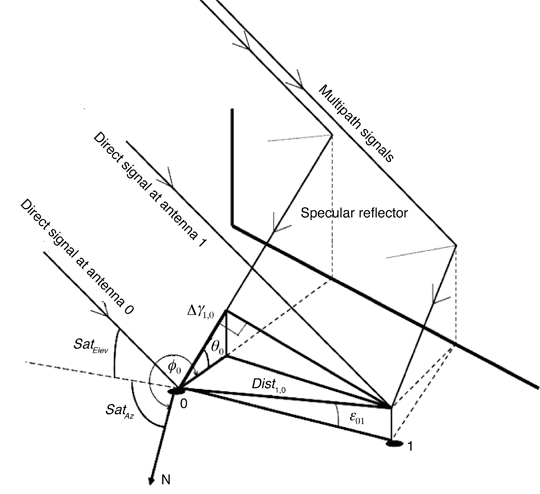
The MIMICS algorithm for a dual-antenna system is based on a specular reflector ray-tracing multipath model (see Figure 1).
Figure 1. 3D ray-tracing modeling of phase multipath for a GNSS dual-antenna system. 0 designates the “master” antenna; 1, the “slave” antenna; Elev and Az, the elevation angle and the azimuth of the satellite, respectively. The other symbols are explained in the text.
After a first step of data synchronization and data-snooping on the data provided by the two receiver antennas, the second step requires the calculation of an approximate position for both antennas, relaxed to a few meters using a standard code solution.
A precise estimation of both antennas’ velocity and acceleration (in real time) is carried out using the carrier-phase observable. Not only should the antenna velocity and acceleration estimates be precisely determined (on the order of a few millimeters per second and a few millimeters per second squared, respectively) but they should also be immune to low-frequency multipath signatures. This is important in our approach, as we use the antennas’ multipath-free dynamic information to separate the multipath in the raw data.
We will start from the basic equations used to derive the single-difference multipath observables.
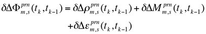
The observation equation for a single-difference between receivers, using a common external clock (oscillator), is given (in distance units) by:
(2)
where m indicates the master antenna; s, the slave antenna; prn, the satellite number; Δ, the operator for single differencing between receivers; Φ, the carrier-phase observation; ρ, the slant range between the satellite and receiver antennas; N, the carrier-phase ambiguity; M, the multipath; and ε, the system noise.
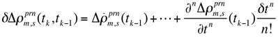
By sequentially differencing Equation (2) in time to remove the single-difference ambiguity from the observation equation, we obtain (as long as there is no loss of lock or cycle slips):
(3)
where
(4)
One of the key ideas in deriving the multipath observable from Equation (3) is to estimate given by Equation (4). We will outline our approach in a later section.
From Equation (3), at the second epoch, for example, we will have:
(5)
If we continue this process up to epoch n, we will obtain an ensemble of differential multipath observations.
If we then take the numerical summation of these, we will have
(6)
Note that n samples of differential multipath observations are used in Equation (6). Therefore, we need n + 1 observations.
Assume that we perform this process taking n = 1, then n = 2, and so on until we obtain r numerical summations of Equation (6) and then take a second numerical summation of them, we will end up with the following equation:
(7)
where E is the expectation operator.
Another key idea in our approach is associated with Equation (7). To isolate the initial epoch multipath, , from the differential multipath observations, the first term on the right-hand side of Equation (7), , should be removed.
This can be accomplished by mechanical calibration and/or numerical randomization. To summarize the idea, we have to create random multipath physically (or numerically) at the initialization step. When the isolation of the initial multipath epoch is completed, we can recover multipath at every epoch using Equation (5).
Digital Differentiators. We introduce digital differentiators in our approach to derive higher order range dynamics (that is, range rate, range-rate change, and so on) using the single-difference (between receivers connected to a common external oscillator) carrier-phase observations. These higher order range dynamics are used in Equation (4).
There are important classes of finite-impulse-response differentiators, which are highly accurate at low to medium frequencies. In central-difference approximations, both the backward and the forward values of the function are used to approximate the current value of the derivative.
Researchers have demonstrated that the coefficients of the maximally linear digital differentiator of order 2N + 1 are the same as the coefficients of the easily computed central-difference approximation of order N.
Another advantage of this class is that within a certain maximum allowable ripple on the amplitude response of the resultant differentiator, its pass band can be dramatically increased. In our approach, this is something fundamental as the multipath in kinematic scenarios is conceptually treated as high-frequency correlated multipath, depending on the platform dynamics and the distance to the reflector(s).
Adaptive Estimation. To derive single-difference multipath at the initial epoch, , a numerical randomization (or mechanical calibration) of the single-difference multipath observations is performed in our approach. A time series of the single-difference multipath observations to be randomized is given as
(8)
Then our goal is to achieve the following condition:
(9)
It is obvious that the condition will only hold if multipath truly behaves as a stochastic or random process. The estimation of multipath in a kinematic scenario has to be understood as the estimation of time-correlated random errors. However, there is no straightforward way to find the correlation periods and model the errors.
Our idea is to decorrelate the between-antenna relative multipath through the introduction of a pseudorandom motion. As one cannot completely rely only on a decorrelation through the platform calibration motion, one also has to do it through the mathematical “whitening” of the time series.
Nevertheless, the ensemble of data depicted in the above formulation can be modeled as an oscillatory random process, for which second or higher order autoregressive (AR) models can provide more realistic modeling in kinematic scenarios. (An autoregressive process is simply another name for a linear difference equation model where the input or forcing function is white Gaussian noise.) We can estimate the parameters of this model in real time, in a block-by-block analysis using the familiar Yule-Walker equations. A whitening filter can then be formed from the estimation parameters.
We obtain the AR coefficients using the autocorrelation coefficient vector of the random sequences. Since the order of the coefficient estimation depends on the multipath spectra (in turn dependent on the platform dynamics and reflector distance), MIMICS uses a cost function to estimate adaptively, in real time, the appropriate order. An order too low results in a poor whitener of the background colored noise, while an order too large might affect the embedded original signal that we are interested in detecting.
The cost function uses the residual sum of squared error. The order estimate that gives the lowest error is the one chosen, and this task is done iteratively until it reaches a minimum threshold value. Once this stage is fulfilled, the multipath observable can be easily obtained.
Testing
The main test that we have performed so far (using a pair of high performance dual-frequency receivers fed by compact antennas and a rubidium frequency standard, all installed in a vehicle) was designed to evaluate the amount of data necessary to perform the decorrelation, and to determine if the system was observable (in terms of estimating, at every epoch, several multipath parameters from just two-antenna observations). Receiver data was collected and post-processed (so-called RTK-style processing) although, with sufficient computing power, data processing could take place in real, or near real, time.
In a real-life scenario, the platform pseudorandom motions have the advantage that carrier-phase embedded dynamics are typically changing faster and in a three-dimensional manner (antennas sense different pitch and yaw angles). Thus a faster and more robust decorrelation is possible.
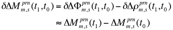
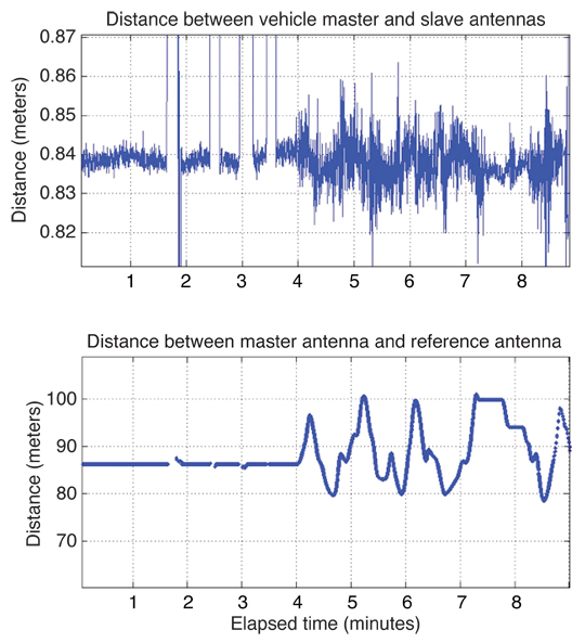
One can see from the bottom picture in Figure 2 the façade of the building behaving as the effective reflector. The vehicle performed several motions, depicted in the bottom panel of Figure 3, always in the visible parking lot, hence the building constantly blocked the view to some satellites. We used only the L1 data from the receivers recorded at a rate of 10 Hz.
In the bottom panel of Figure 3, one can also see the kind of motion performed by the platform. Accelerations, jerk, idling, and several stops were performed on purpose to see the resultant multipath spectra differences between the antennas. The reference station (using a receiver with capabilities similar to those in the vehicle) was located on a roof-top no more than 110 meters away from the vehicle antennas during the test. As such, most of the usual biases where removed from the solution in the differencing process and the only remaining bias can be attributed to multipath. The data from the reference receiver was only used to obtain the varying baseline with respect to the vehicle master antenna.
In the top panel of Figure 3, one can see the geometric distance calculated from the integer-ambiguity-fixed solutions of both antenna/receiver combinations. Since the distance between the mounting points on the antenna-support bar was accurately measured before the test (84 centimeters), we had an easy way to evaluate the solution quality. The “outliers” seen in the figure come from code solutions because the building mentioned before blocked most of the satellites towards the southeast. As a result, many times fewer than five satellites were available.
Figure 3. Correlation between vehicle dynamics (heading angle) and the multipath spectra.
Looking at the first nine minutes of results in Figure 4, one can see that when the vehicle is still stationary, the multipath has a very clear quasi-sinusoidal behavior with a period of a few minutes. Also, one can see that it is zero-mean as expected (unlike code multipath). When the vehicle starts moving (at about the four-minute mark), the noise figure is amplified (depending on the platform velocity), but one can still see a mixture of low-frequency components coming from multipath (although with shorter periods).
These results indicate, firstly, that regardless of the distance between two antennas, multipath will not be eliminated after differencing, unlike some other biases. Secondly, when the platform has multiple dynamics, multipath spectra will change accordingly starting from the low-frequency components (due to nearby reflectors) towards the high-frequency ones (including diffraction coming from the building edges and corners). As such, our approach to adaptively model multipath in real time as a quasi-random process makes sense.
Figure 4. Position results from the kinematic test, showing the estimated distance between the two vehicle antennas (upper plot) and the distance between the master antenna and the reference antenna.
Multipath Observables. The multipath observables are obtained through the MIMICS algorithm. It is quite flexible in terms of latency and filter order when it comes to deriving the observables. Basically, it is dependent on the platform dynamics and the amplitude of the residuals of the whitened time series (meaning that if they exceed a certain threshold, then the filtering order doesn’t fit the data).
When comparing the observations delivered every half second for PRN 5 with the ones delivered every second, it is clear that the larger the interval between observations, the better we are able to recover the true biased sinusoidal behavior of multipath. However, in machine control, some applications require a very low latency. Therefore, there must be a compromise between the multipath observable accuracy and the rate at which it is generated.
Multipath Parameter Estimation. Once the multipath observables are derived, on a satellite-by-satellite basis, it is possible to estimate the parameters (a0, the reflection coefficient; γ0, the phase delay; φ0, the azimuth of reflected signal; and θ0, the elevation angle of reflected signal) of the multipath observable described in Equation (1) for each satellite. As mentioned earlier, an EKF is used for the estimation procedure.
When the platform experiences higher dynamics, such as rapid rotations, acceleration is no longer constant and jerk is present. Therefore, a Gauss-Markov model may be more suitable than other stochastic models, such as random walk, and can be implemented through a position-velocity-acceleration dynamic model.
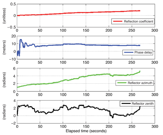
As an example, the results from the multipath parameter estimation are given for satellite PRN 5 in Figure 5. One can see that it takes roughly 40 seconds for the filter to converge. This is especially seen in the phase delay.
Converted to meters, the multipath phase delay gives an approximate value of 10 meters, which is consistent with the distance from the moving platform to the dominant specular reflector (the building’s façade).
Figure 5. PRN 5 multipath parameter estimation.
Multipath Mitigation. After going through all the MIMICS steps,
from the initial data tracking and synchronization between the dual-antenna system up to the multipath parameter estimation for each continuously observed satellite, we can now generate the multipath corrections and thus correct each raw carrier-phase observation.
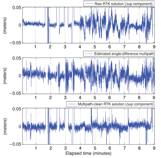
One can see in Figure 6 three different plots from the solution domain depicting the original raw (multipath-contaminated) GPS-RTK baseline up-component (top), the estimated carrier-phase multipath signal (middle), and the difference between the two above time series; that is, the GPS-RTK multipath-ameliorated solution (bottom). A clear improvement is visible. In terms of numbers, and only considering the results “cleaned” from outliers and differential-code solutions (provided by the RTK post-processing software, when carrier-phase ambiguities cannot be fixed), the up-component root-mean-square value before was 2.5 centimeters, and after applying MIMICS it stood at 1.8 centimeters.
Figure 6. MIMICS algorithm results for the vehicle baseline from the first 9 minutes of the test.
Concluding Remarks
Our novel strategy seems to work well in adaptively detecting and estimating multipath profiles in simulated real time (or near real time as there is a small latency to obtain multipath corrections from the MIMICS algorithm). The approach is designed to be applied in specular-rich and varying multipath environments, quite common at construction sites, harbors, airports, and other environments where GNSS-based heading systems are becoming standard. The equipment setup can be simplified, compared to that used in our test, if a single receiver with dual-antenna inputs is employed.
Despite its success, there are some limitations to our approach. From the plots, it’s clear that not all multipath patterns were removed, even though the improvements are notable. Moreover, estimating multipath adaptively in real time can be a problem from a computational point of view when using high update rates. And when the platform is static and no previous calibration exists, the estimation of multipath parameters is impossible as the system is not observable. Nevertheless, the approach shows promise and real-world tests are in the planning stages.
Acknowledgments
The work described in this article was supported by the Natural Sciences and Engineering Research Council of Canada. The article is based on a paper given at the Institute of Electrical and Electronics Engineers / Institute of Navigation Position Location and Navigation Symposium 2010, held in Indian Wells, California, May 6–8, 2010.
Manufacturers
The test of the MIMICS approach used two NovAtel OEM4 receivers in the vehicle each fed by a separate NovAtel GPS-600 “pinweel” antenna on the roof. A Temex Time (now Spectratime) LPFRS-01/5M rubidium frequency standard supplied a common oscillator frequency to both receivers. The reference receiver was a Trimble 5700, fed by a Trimble Zephyr geodetic antenna.
Luis Serrano is a senior navigation engineer at EADS Astrium U.K., in the Ground Segment Group, based in Portsmouth, where he leads studies and research in GNSS high precision applications and GNSS anti-jamming/spoofing software and patents. He is also a completing his Ph.D. degree at the University of New Brunwick (UNB), Fredericton, Canada.
Don Kim is an adjunct professor and a senior research associate in the Department of Geodesy and Geomatics Engineering at UNB where he has been doing research and teaching since 1998. He has a bachelor’s degree in urban engineering and an M.Sc.E. and Ph.D. in geomatics from Seoul National University. Dr. Kim has been involved in GNSS research since 1991 and his research centers on high-precision positioning and navigation sensor technologies for practical solutions in scientific and industrial applications that require real-time processing, high data rates, and high accuracy over long ranges with possible high platform dynamics.
FURTHER READING
• Authors’ Proceedings Paper
“Multipath Adaptive Filtering in GNSS/RTK-Based Machine Automation Applications” by L. Serrano, D. Kim, and R.B. Langley in Proceedings of PLANS 2010, IEEE/ION Position Location and Navigation Symposium, Indian Wells, California, May 4–6, 2010, pp. 60–69, doi: 10.1109/PLANS.2010.5507201.
• Pseudorange and Carrier-Phase Multipath Theory and Amelioration Articles from GPS World
“It’s Not All Bad: Understanding and Using GNSS Multipath” by A. Bilich and K.M. Larson in GPS World, Vol. 20, No. 10, October 2009, pp. 31–39.
• Dual Antenna Carrier-phase Multipath Observable
“A New Carrier-Phase Multipath Observable for GPS Real-Time Kinematics Based on Between Receiver Dynamics” by L. Serrano, D. Kim, and R.B. Langley in Proceedings of the 61st Annual Meeting of The Institute of Navigation, Cambridge, Massachusetts, June 27–29, 2005, pp. 1105–1115.
“Mitigation of Static Carrier Phase Multipath Effects Using Multiple Closely-Spaced Antennas” by J.K. Ray, M.E. Cannon, and P. Fenton in Proceedings of ION GPS-98, the 11th International Technical Meeting of the Satellite Division of The Institute of Navigation, Nashville, Tennessee, September 15–18, 1998, pp. 1025–1034.
• Digital Differentiation
“Digital Differentiators Based on Taylor Series” by I.R. Khan and R. Ohba in the Institute of Electronics, Information and Communication Engineers (Japan) Transactions on Fundamentals of Electronics, Communications and Computer Sciences, Vol. E82-A, No. 12, December 1999, pp. 2822–2824.
• Autoregressive Models and the Yule-Walker Equations Random Signals: Detection, Estimation and Data Analysis by K.S. Shanmugan and A.M. Breipohl, published by Wiley, New York, 1988.
• Kalman Filtering and Dynamic Models Introduction to Random Signals and Applied Kalman Filtering: with MATLAB Exercises and Solutions, 3rd edition, by R.G. Brown and P.Y.C. Hwang, published by Wiley, New York, 1997.
Developments in the LightSquared saga came fast and furious in June; highlights are listed below and briefly recapped in the adjacent news story. It will be dated by the time you receive this issue, as it went to press three weeks prior.
For current events, see Top Story and Latest News, and the full versions of stories abridged here. The Navigate, Survey Scene, and GNSS Design & Test e-newsletters, free at env-gpsworld-integration.kinsta.cloud/subscribe, will keep you up to date.
In chronological order, from late May to late June:
LightSquared Las Vegas Test Towers Flawed, FCC Filing Shows
House Bill Ensures FCC Takes No Action that Would Harm Military Use of GPS
Test Data Shows LightSquared Slams Medium, High-Precision GPS Receivers
PNT Advisory Board Finds Interference, Says Move It
LightSquared, FCC Rebuttals Distort Record
NPEF Report on Military Receivers Calls for FCC Recision
LightSquared Asks for, Receives Extension on Final Interference Report
Claims of LightSquared Solution Discounted
Air Transport Association Tells Congress to Protect GPS
Interference with GPS Poses Major Threat to U.S. Economy
LightSquared Applies to International Telecommunications Union for Global Signal
Flawed Test Towers
Results from a key round of field tests conducted near Las Vegas, Nevada, may show overly optimistic results regarding the effects of the LightSquared terrestrial signal on GPS receivers. According to a LightSquared addendum filed with the Federal Communications Commission (FCC) a week after the May 16 Working Group report, the company’s equipment broadcast during the tests at lower-than-planned levels for its eventual deployment across the United States. Further, LightSquared may not currently be prepared or equipped to broadcast according to the terms of its business plan or its conditional waiver.
LightSquared does not appear to have developed the full software suite nor possess the full equipment to implement the plan the company says has been in preparation for many years. Critical testing was conducted under conditions that do not truly replicate what may be the case should the FCC allow the plan to go forward.
House Bills Target the Waiver
On May 27, the U.S. House of Representatives passed a bill stating that the FCC shall not provide final authorization for LightSquared operations until Defense Department concerns about GPS interference have been resolved. The bill then went to the U.S. Senate for its action.
On June 23, the House Appropriations Committee approved action that would stop the FCC from expending any funds related to the LightSquared conditional waiver until all concerns have been resolved about interference with GPS. The amendment passed in a unanimous voice vote by the full committee, underscoring growing congressional concern about harm to GPS.
The House actions and a letter to the FCC signed by 32 U.S. senators may presage a showdown over the issue between Congress and the president, who has promised increased broadband access. A 4G wireless network providing this access could be facilitated by LightSquared sales of service via its tower transmitters to wireless carriers. LightSquared has already signed a $20 billion, 15-year deal with Sprint.
Tests Slam High-Precision Receivers
Data from Las Vegas field tests show that wide-bandwidth, high-precision GPS receivers started feeling the effects of the LightSquared transmission about 1,800 meters from the tower. Medium-bandwidth high-precision GPS receivers started feeling the effects of the LightSquared transmission at about 1,200 meters from the tower. In each case, there was about a 200-meter buffer from when the GPS receivers started to feel the effects of the LightSquared transmission to the GPS receiver being jammed, at 1,600 meters and 1,000 meters respectively.
GPS World has received further details of the tests but has not been authorized to publish them yet.
Deere & Company, a major provider of precision agriculture equipment and services, notified the FCC on May 26 of substantial interference with its GPS receivers by the LightSquared signal. Deere receivers registered impact of and interference by the LightSquared signal as far away as 22 miles from a transmitter. Further, the company has found no practicable technical solution to the problem.
PNT Advisory Board: Move ATC
At its June 9–10 meeting, the National Space-Based Positioning, Navigation and Timing (PNT) Advisory Board found that GPS services cannot be assured if the LightSquared plan is approved, and that the only viable option for continued availability of GPS as well as new wireless broadband is to find another spectrum for LightSquared not adjacent to the GPS frequency.
The formal recommendation reads: “The provision of GPS services cannot be assured if the LightSquared proposal for satellite and terrestrial broadband provision using the MSS L-Band receives final approval.
“The only reasonable and viable option to continue ubiquitous availability of GPS and the provision of a new 4G wireless broadband capability would be for the FCC to assign an alternate frequency spectrum to LightSquared that has little or no probability of affecting the delivery or utilization of GPS/GNSS services.”
During the discussion, one advisory board member, a former goveronor of the state of Wyoming, told presenter Jeff Carlisle of LightSquared, “Your definition of mitigation seems more tied to a legal argument than a common-sense argument.”
Rebuttals Distort Record
Claims by LightSquared’s Carlisle and FCC chair Julius Genachowski, that the GPS industry knew long ago about LightSquared’s plan for powerful terrestrial transmitters, contradict the truth. Examination of FCC filings show that the GPS industry knew about and agreed to a plan by a previous ownership of the company, for a different purpose, with a different business concept, and employing a completely different technological approach, one that would not have harmed GPS transmissions and disabled GPS users the way the current LightSquared plan does.
The terrestrial broadband operations first unveiled in November 2010 cannot be described as ancillary to the purpose for which Lightsquared predecessors Motient, MSV, and SkyTerra received their spectrum and licenses — that is, to provide a service that was primarily a mobile satellite service. The November letter to the FCC described a new business model that turns the original concept on its head. LightSquared for the first time revealed plans to build a “nationwide network of 40,000 terrestrial base stations,” and stated that “the capacity of its fully deployed terrestrial network across all base stations will be tens of thousands of times the capacity of either of [its] satellites.”
The deviations from established policy required to accommodate LightSquared’s new business model are not technicalities. They represent a fundamental change to a complex and interrelated set of rules that were carefully designed to protect GPS users from interference.
The predecessor companies had to protect their own primary satellite operations from interference. The protection that their own satellite operations required was also sufficient — at that time — to protect GPS receivers. The terrestrial network and powerful signal LightSquared now proposes bear no resemblance to the operations the FCC authorized in 2003.
Military Report Calls for FCC Retreat
The National PNT Engineering Forum concluded after testing classified and GPS receivers under LightSquared terrestrial transmission conditions: “Significant concerns remain that operation of an ATC integrated service as originally envisioned by the FCC cannot successfully coexist with GPS.”
The NPEF report calls for rescinding the FCC waiver for LightSquared terrestrial transmissions, conducting more thorough studies on impacts, and revisiting the 2003–2010 authorizations. The group tested a variety of military receivers under classified categorization, also known as “government receivers.”
Final Report Withheld
At the last minute of a June 15 deadline for the final Working Group report on interference, LightSquared asked for a two-week extension. Federal regulators granted the request, and the final report is now due on July 1.
A spokesperson for the Coalition to Save Our GPS revealed that “The Working Group results show devastating interference to GPS and no proven method of mitigation. Delay will not change these results. These results are the same results the FCC had had before it granted the waiver.”
Some Solution. Three days after requesting the delay, LightSquared announced it had solved the problem, by proposing to broadcast only from the lower end of its permitted spectrum band. GPS experts countered that this would still disable the functioning of high-precision receivers.
Air Transport Opposes Waiver
The Air Transport Association and the Aircraft Owners & Pilots Association told Congress that the only acceptable mitigation is for LightSquared’s operations to be moved outside of the L-band and away from GPS. “With so much of the early evidence showing that LightSquared’s proposed network would potentially endanger nearly every flight operating in U.S. airspace, it seems evident that no further development of this system can be allowed.”
Going Global
LightSquared has filed documents relative to the International Telecommunications Union, signaling intent to use its entire band at the full authorized power. The company’s goal appears to be to work internationally, circumventing U.S. regulation, to obtain permits to broadcast a terrestrial signal globally.
By Jenna R. Tong, Robert J. Watson, and Cathryn N. Mitchell, University of Bath
Using signal-to-noise measurements from a single commercial-grade L1 GPS receiver, it is possible to detect interference or jamming that is above the thermal noise floor and below a power that causes loss of position.
Interference, intentional or unintentional, is an acknowledged vulnerability of GPS systems. Many of the potential sources of interference are unintentional: interference can caused by harmonics of out-of-band signals, electronic noise, or malfunctioning equipment. The effect, however, is the same independent of intent.
The presence of high-power interference which causes continual denial of service is fairly easy to detect, but lower power interference may still degrade performance, for example by causing loss of lock on some satellites, thus increasing position dilution of precision, although the receiver continues to output a position. Short periods of denial of service caused by intermittent high-power interference may not be immediately detected depending on the timing and ability of the system in use to deal with temporary loss of signal.
Therefore, to fully characterize an antenna environment requires a 24/7 system, whether the purpose is to determine whether a location is suitable prior to installation, to identify whether problems at an existing site are due to interference, or to provide warnings of the presence of interference on a continuous basis. In particular, information on timing — for example finding a time of day or day of the week when interference is regularly seen — may assist in determining the source of the interference.
This research forms part of the GNSS Availability Accuracy Reliability anD Integrity Assessment for timing and Navigation (GAARDIAN) project, which provides a mesh of sensors to monitor the integrity, reliability, continuity, and accuracy of the locally received GPS (or other GNSS) and eLoran signals continuously and to detect anomalous conditions such as local interference, differentiating between possible sources of errors such as interference, multipath, satellite errors, or space weather.
Here we look at using the signal-to-noise ratio (SNR) values from a single-frequency GPS receiver to detect interference. There are two stages to the algorithm: determining the local environment of the antenna in terms of multipath and interference, and identifying and recording potential interference events.
Since this method uses values output from a GPS receiver, characterizing the response to interference of the receiver used in the probe is necessary, to indicate what level interference can be detected with the system, as well as ensuring that false positives are not produced, and the effects of interference can be separated from those of multipath and scintillation, which can also cause decreases in SNR.
We used a commercial, single-frequency receiver, recording this data from NMEA messags for analysis:
SNR, in dB, reported as an integer
elevation, in degrees, reported as an integer
azimuth, in degrees, reported as an integer
carrier lock time, in seconds.
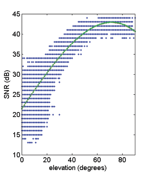
Algorithm. To determine the presence of interference, the normal state of the receiver must first be calculated. Initially it is assumed the receiver is fixed with an unchanging multipath environment. SNR and elevation values from all satellites are accumulated for several hours. To reduce influence of the unknown multipath environment, values from satellites below 10 degrees elevation and from those where the carrier lock time is less than four minutes are removed from the data set.
A polynomial fit between elevation and SNR is then calculated from the remaining data. A second- or third-degree polynomial generally fits the high-elevation data with deviations from the profile at low elevations being primarily due to multipath where interference is not present.
The standard deviation of SNR at each elevation is then calculated. The combination of the polynomial and these values of standard deviation characterize the normal environment of the receiver, for the case where interference is not present in the data gathered (Figure 1).
Figure 1. Raw SNR data against elevation, for all satellites in view over a period of 12 hours (blue), and a polynomial fitting to the same data (green).
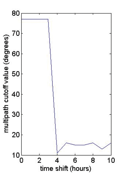
To confirm that the threshold values returned by the first stage of the algorithm are valid, a value is calculated for the elevation where the SNR value drops below the polynomial curve by the greatest amount.
If interference is not present, this is normally found at the point where multipath begins to influence the incoming signal and can be considered as a rough multipath cutoff, used to remove signals that may be influenced by multipath from later stages of the analysis.
Assuming a well-sited antenna, a value greater than 25 degrees for this value indicates the possible presence of interference in the data used to calculate the polynomial. In cases where this value is high, the data in question would be rejected, and optionally a user may be warned that there may be pre-existing interference. If the antenna-receiver combination has been previously calibrated in a known good environment, it would be also possible to identify interference based on the difference in polynomial and standard deviation values between that environment and the location being tested.
Figure 2 shows the value of this multipath cutoff (in degrees) for a set of data where interference was known to be present initially, against the start time for the data used to calculate the polynomial and multipath cutoff values, by number of hours from the start of the file.
Once the mask is developed, a threshold value can be set to be n standard deviations below the polynomial, and events are detected by the combination of:
At least four satellites with elevations above the multipath cutoff which are below the threshold value or which were above the multipath cutoff previous to losing lock.
This status is continuous for more than a set time t.
Requiring multiple satellites limits the effects of other influences on SNR such as multipath; requiring an extended time period removes very short-term fluctuations.
The number of false positives and the power of interference required to cause an alarm then depends primarily on the value of the threshold factor n, and on the time period t, which here we kept at a constant of 30 seconds.
Testing
To avoid radiating interference, we constructed an RF network to facilitate injection of jamming signals into the GPS signal path. The GPS signal from a roof-mounted choke-ring antenna was passed through an amplifier and attenuator chain to provide 0 dB forward gain, but around 40 dB reverse isolation. An additional stepped attenuator (0–40 dB in 1 dB steps) was also included. The buffered signal from the antenna was then combined with the output of a vector signal generator used to provide the jamming signal.
The combined signal was then fed into the GPS receiver via a DC-block to remove the antenna bias voltage. The signal generator is capable of producing a wide variety of jamming including matched spectrum wideband noise, CW, and pulsed signals. The adjustment of both the signal generator output power and the signal attenuator a
llow the replication of a variety of signal-to-noise and jammer-to-noise scenarios.
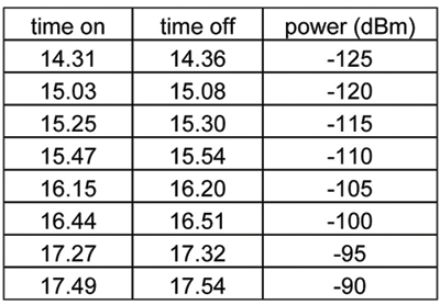
With the receiver locked onto a stable position, CW signals at L1 frequency were introduced into the receiver at levels from –125 dBm to –90 dBm in steps of 5 dBm, with at least 15 minutes of buffer time for the receiver to recover between each step (Table 1). Data was logged at 1 Hz throughout. We collected 20 hours of data, to calculate threshold values from data with no known interference.
Table 1.
Results
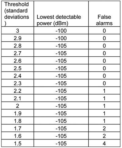
Twelve hours of data from a period where no known interference was present was used to form the SNR mask, and events longer than 30 seconds were looked for using various values of n for the threshold across all 20 hours of data. A false alarm was considered to be any event where interference was detected while the signal generator was off. Table 2 summarizes the response for different threshold levels.
Table 2.
In this test, CW interference of –100 dBm was required before the number of satellites with carrier lock dropped below four even for a single epoch, and –90 dBm was required to cause a sustained loss of lock, but jamming of –105 dBm was still detectable by this system with no false positives returned.
Decreasing the threshold began to produce false positives without detecting the smaller interference signals. This is not surprising as the thermal noise floor, assuming 2 MHz bandwidth, is about –110 dBm.
In the raw data from the detected events, a sharp dip in SNR is often seen at the beginning of an event, followed by recovery as the receiver compensates. In this particular case, where the aim is to detect the interference, this could lead to interference going undetected if the initial sharp dip was underneath the time threshold (30 seconds) and the recovery took the SNR of some of the satellites above the SNR threshold (Figure 3).
Figure 3. Value of polynomial mask (blue) and actual SNR (red) as recorded for four satellites during the period around the injection of the -100 dBm CW signal, showing initial dip and partial recovery.
Conclusion
Using only SNR values from a low-cost L1 GPS receiver, it is possible to detect CW interference which is above the thermal noise floor and below a power that causes loss of position. Different types of interference are expected to produce a different response, and unintentional interference is likely to be broadband or not directly centered on L1. The antenna used may also have a strong effect. These factors have not been examined here, although in practice the algorithm has run in multiple locations with different antennas, both direct and via splitters.
Regardless of the precise type of interference, the system would be expected to detect any interfering signal which impacts the SNR of the receiver, and to do so even if the signal strength was below a level which caused denial of service in that area.
The results are specific to the receiver used and its response to interference, although the algorithm would be capable of using data from any receiver that provided SNR values. Ideally the system used for measurement would have little or no built-in interference rejection.
Although this data was collected and then examined after the fact for signs of interference, the system works in precisely the same way in real time. Further trials will test the algorithm’s performance in real time and with different jamming scenarios, and compare results from multiple receivers in a single location and the performance of the algorithm with different antennas.
Acknowledgments
This work was funded by the Engineering and Physical Sciences Research Council and the Technology Strategy Board.
Jenna R. Tong is a postdoctoral researcher in electronic and electrical engineering at the University of Bath. Her Ph.D. in electron tomography is from the University of Cambridge.
Robert J. Watson received a Ph.D. degree in electronic engineering from the University of Essex, and is senior lecturer in electronic and electrical engineering at the University of Bath.
Cathryn N. Mitchell is a professor of engineering at the University of Bath and the Director of Invert Centre for Imaging Science. She received a Ph.D. from the University of Wales Aberystwyth.
The recent broadcast of the first CDMA signal from the new GLONASS-K satellite culminates a long series of events that began in 1989. A key participant gives a first-hand account of the history of many meetings, formal and informal, that created true interoperability between the two major satellite systems, giving users a modern GNSS in action.
October 18, 1989, the Queen Elizabeth Auditorium in London, around 8:30 am. Unknown to me, two 60-minute periods were about to imprint themselves indelibly on my memory.
I walked up the stairs to the exhibition booth of my company, Ashtech, at The Royal Institute of Navigation conference. My good friend, the late Ann Beatty, met me and asked, “Any news from home?”
I thought it was just a casual customary question, and replied: “Thanks, all OK.” She had a strange look on her face. She continued: “Are all your family really OK?” I replied again: “Thanks, all good.” She then realized that I had no clue about the cataclysmic event that had hit the San Francisco Bay area. She abruptly said, “Don’t you know? The big one came! The big earthquake hit San Francisco!”
Californians know the rumors that when The Big One comes, Nevada will have ocean frontage. Now she was telling me that The Big One came! I rushed to the phone, and the recorded AT&T message said, “All lines to your area are out of service.” It took me another hour to find out that this was not yet The Big One, and that my family was safe. I will never forget these 60 minutes of my life. Never!
Nor will I ever forget the events of the next 60 minutes.
After the stress had settled a bit, a delegation from the Russian Space Agency visited our booth. First they expressed their sympathy regarding the earthquake. Then we discussed GPS technology and its similarities with GLONASS. Both systems were fairly new then, although GPS had started first, with a Block I launch in 1978, followed by GLONASS with a launch in 1982. At the time we met in London, GPS was flying 12 satellites, and GLONASS also had 12 in orbit.
The Russian delegation visited all GPS manufacturers’ booths in the exhibition hall and then gathered in the coffee area for their private discussions. A few hours before the conference closed, they returned to our booth and said, “We want to combine GPS and GLONASS, and you are our first choice.” Simply put, I was fascinated and excited.
After working out visa and travel details, four months later I arrived in Moscow in the cold days of February 1990. It was still the Soviet Union.
I had grown up in Iran where the U.S.S.R. was our neighbor to the north. Remembering the global political landscape of my childhood days, I felt both fascination and fear as my airplane landed at Moscow airport.
Upon meeting the people who greeted me at the airport, my fears disappeared, and my fascination grew stronger.
Our first formal meeting took place in the Institute of Space Device Engineering (ISDE), a division of the Russian Space Agency that was responsible for the GLONASS program. The opening photo shows me with the late Dr. Nikolay Yemelianovich Ivanov, director of the GLONASS program, at that first meeting.
I want to focus a bit on the GLONASS team and applaud them for their efforts. What makes the GLONASS team special is that they worked under much harder political and financial conditions than the GPS or Galileo teams. But still they were able to make the project successful. The Soviet Union and later Russia went through huge political, economic, social, and geographical revolutions, but the GLONASS team managed to keep the satellite navigation program alive and successful.
Galileo’s management, while enjoying much more stability and financial luxury, can certainly appreciate and understand the significance of what the GLONASS team accomplished. Galileo also benefitted from the European integration of 27 countries, while the Soviet Union disintegrated into 15 separate nations.
Despite all their heroic work, individuals on the GLONASS team have received almost no international recognition. At home they went unnoticed, due to their political situations. For example, the highest international recognition that Dr. Ivanov received was that he became a member of the GPS World Advisory Board, which I facilitated. In this article, I want to salute some members that I know and at least keep their names and photos recorded in the GPS World archives.
In the first meeting, everyone recognized and emphasized the great potential of combining GPS and GLONASS for a variety of applications. I became more assured of the deep desires of my hosts to make this happen. They had prepared detailed charts and plans, especially for high-precision applications. They also gave me the GLONASS Interface Control Document (ICD) for the first time.
We signed a cooperation protocol and agreed to explore technical details in our next meeting, which occurred a few months later. There I began to know Dr. Stanislav “Stas” Ulianovich Sila-Navitsky, at that time the chief scientist of Dr. Ivanov’s team. Later he became my vice president in three companies that I founded. He also became my best friend of 19 years, before he passed away on May 7, 2010.
We had several meetings in Moscow and one in Paris in the headquarters of our partner SAGEM.
I have wonderful memories of all the meetings. One meeting in Paris included General Leonid Ivanovich Gusev, the head of ISDE. One evening Stas called my hotel room and asked me to cancel our dinner at a famous French restaurant and instead join them for a “real dinner.” Apparently General Gusev was tired of French food! The real dinner took place in the General’s hotel room, and the menu consisted of dark Russian bread, Russian kielbasa sausage, Russian seledka herring, and an abundance of Russian vodka.
Our first announcement of combining GPS and GLONASS was published in GPS World magazine, in only its second issue, March/April 1990. That year we had a poster banner in our Institute of Navigation exhibition, showing the American flag and the Soviet flag (hammer and sickle) next to each other. My very good friend, Colonel Gaylord Green, the second director of the GPS Joint Program Office, refused to have his picture taken with me in front of that banner. Instead, we stood over to another side of the booth for his photo.
A few months after the Paris meeting, the political process known as perestroika began and caused the Soviet Union to end. Life became extremely difficult for Russians.
I called Stas to discuss the situation. We concluded that we had no choice but to continue the plan on our own if we wanted to combine GPS and GLONASS. I went back to Moscow several times, and in February 1992 officially opened the Moscow office of Ashtech. This office is still operational in Moscow with about 10 percent of the original team. It is now in the process of being purchased by Trimble Navigation. What a turn of events!
In 1996 we introduced the first combined GPS and GLONASS receiver; the product announcement appeared in GPS World, July 1996
Back home in the United States, the situation was different. Supporting GLONASS was an unpatriotic act. The most prominent figures of GPS teased me for wasting my time with GLONASS. The news favored their arguments: the Russian economy was going downhill. In September 1998, the Russian ruble collapsed more than 300 percent within a week. Banks closed. Even Coca Cola was not able to pay its employees in Russia because of bank closures. Many western companies left Russia. During that period, I intentionally stayed longer times in Moscow and managed to pay our employees without a day of delay. Furthermore, a more than three-fold rate change in favor of the dollar made our employees relatively rich, because their salaries were based on the U.S. dollar.
I remained confident that GLONASS would succeed because I had seen the enthusiasm and dedication of GLONASS management and engineers.
My Ashtech partners wanted to take the company public to recoup their investments. They thought Wall Street would negatively view GLONASS and the Russian connection. So my aspiration did not match theirs, and I started Javad Positioning System (JPS) in 1996. About 90 percent of the staff engineers followed me to JPS.
One of John Scully’s vice presidents did to Ashtech what Scully did to Apple. Meanwhile JPS became very successful, as Apple did when Steve Jobs returned.
Subsequent to another event and termination of some obligations and commitments, I started JAVAD GNSS in June 2007. Almost all of the key people followed me again. Our current team has a history of working together for close to 20 years.
In JAVAD GNSS we raised the bar of GPS/GLONASS integration to a higher level and focused in two new directions. The first was to eliminate the problem of GLONASS inter-channel biases, which is inherent to the GLONASS frequency-division multiple access (FDMA) signal structure. The second was to support the opinion of GLONASS engineers who were pushing for a new code-division multiple access (CDMA) signal for GLONASS, similar to the GPS signal.
We resolved the GLONASS inter-channel biases issue around 2009 and announced, “Our GLONASS is as good as GPS.”
On the second front, we worked with the top managements of ISDE and the Information Analysis Center (IAC) of the Russian Space Center to demonstrate the advantages of CDMA for high-precision applications.
Some years ago, Stas had confided in me that the issue of CDMA was nothing new, and had been extensively deliberated at all levels of various GLONASS organizations during the early design phase of the system. The result of all these discussions was that engineers and technical people favored CDMA, but the higher management, mostly influenced by the military organizations, held out for FDMA. The reason for favoring FDMA is still a secret, though some believe that they just wanted to be different from GPS and did not see much advantage in CDMA. Some also believed FDMA gave better jamming protection.
Of course in those very early days, no one imagined using GPS or GLONASS for high-precision applications, and as such truly there was not much difference between CDMA and FDMA. Much later, the notion of using carrier phase of GPS and GLONASS signals for high-precision applications was discovered, and then the advantages of CDMA became relevant, as Dr. Ivanov also hinted in our first meeting.
After we combined GPS and GLONASS, and as a lot of our worldwide users began comparing the two systems, the issue of CDMA versus FDMA again came up for discussion among the GLONASS authorities.
More recently, since 2007, we had several meetings in the offices of ISDE in Moscow, in IAC in Korolev (the Russian Space City), and several in our JAVAD GNSS office in Moscow. Most importantly, we had several meetings in my Moscow apartment, enhanced by Russian vodka and the best Armenian cognac, courtesy of Sergey Revnivykh, head of IAC. All meetings were open and candid, discussing and demonstrating the advantages of CDMA, in support of the ISDE engineers who were reluctant to express their opinion above certain levels.
I also met with the head of the Russian Space Agency, Dr. Anatoly Nikolayevich Perminov, who personally supported and sponsored me in obtaining an extended Russian residency visa. Let me also express my appreciation for receiving the Medal of Honor from the Russian Cosmonauts Federation, along with the official astronaut watch. I don’t understand the reason for receiving a Kalashnikov AK-47 semi-automatic rifle from ISDE for my birthday. I wonder how I can transport it home!
General Anatoly Shilov (deputy director of the Russian Space Center), Dr. Vicheslav Dvorkin (GLONASS deputy general designer), Sergey Revnivykh, Viktor Kosenko (first deputy of chief GLONASS designer) and Sergey Karutin (GLONASS senior scientist) are the new generation of GLONASS leaders who deserve credit for supporting CDMA on GLONASS. Recently, a new GLONASS-K sat-ellite was launched, transmitting an experimental CDMA signal in addition to the legacy signals. Almost immediately, we announced tracking of the new GLONASS-K satellite and its new L3 signal details, hours after it started transmitting. See GPS World archives and our website for details of this signal which seems, in all aspects, as good as GPS.
Another new issue of significant international concern was a new frequency for GLONASS. This issue was more political than technical, and is discussed under the umbrella of interoperability.
In the early days of my frequent travels to Russia, the KGB probably suspected that I was a CIA agent — and the CIA probably suspected that I was a KGB agent! I would not be surprised if both the CIA and KGB monitored every bit of my travels and activities. After some years, the San Francisco airport authorities stopped interrogating me for my activities in Russia any time I came back home. Perhaps because of their deep investigations, I earned the trust and friendship of both sides, and their confidence that I had nothing in mind other than helping to integrate GPS and GLONASS. I was an unofficial member and friend of both U.S. and Russian delegations during the so-called interoperability discussions since 2007, which sometimes touched on the CDMA issue as well.
Some of the most fruitful and friendly discussions between the U.S. and Russian delegations occurred in my apartment in Moscow, after their official meetings. Ken Hodgkins of U.S. State Department; Mike Shaw, director of the National Space-Based Positioning, Navigation, and Timing Coordination Office; David Turner, director of the Center for Space Policy & Strategy; Scott Feairheller of the U.S. Air Force; and Tom Stansell, consultant to the GPS Wing were some of my honored guests.
The new GLONASS frequency discussions are still in progress, and I am proud to host and support both sides the best that I can. Sometimes it is fun to observe that discussions resemble poker games where hands are known to all sides, but players still try to bluff each other! Let’s leave it at that for now.
In May of this year, I had a conversation with General Anatoly Shilov, now second-in-command of the Russian Space Agency, reporting to the first deputy of the minister of defense, General Vladimir Popovkin, who recently replaced Dr. Perminov as head of the Russian Space Center. This is an indication of increased attention and support from the Russian government to its GLONASS program. In our conversation, General Shilov was enthusiastic and optimistic that the GLONASS program will move forward faster.
GLONASS has proven to be a real and reliable complement to GPS. If it were not for the failure of the launch of three GLONASS satellites in December 2010, its constellation would be complete and fully, globally operational today. It will happen soon. Sergey Revnivykh estimates that currently the system has 99.8 percent global coverage.
Today, a truly reliable and fast RTK is not possible without combining GPS and GLONASS satellites.
The most recent testimony to the success of GLONASS comes from the long-time GLONASS opponents who once criticized me for supporting the system. Recently they had to pay a lot of money to acquire the first company that I founded in Moscow, which they believed would never survive.
This year at JAVAD GNSS, I and most of my original employees and GLONASS designers are celebrating our 20th year in Russia, and we are working harder to make the integration of GPS and GLONASS even better.
On May 7, 2010, Stas lost to leukemia. He was not present to witness the successful introduction of our TRIUMPH-VS receivers. My refrigerators in Moscow are full of medicines that he brought for me any time I had a little cold. I miss him a lot, and our team is dedicated to following the path that Stas loved so much.
I want to briefly summarize the current status and the future of GPS and GLONASS from the users’ point of view.
GLONASS now has 24 satellites transmitting FDMA signals in two frequency bands. The failure in the last launch to deploy three more satellites delayed completion of the constellation to the end of 2011. The good thing about GLONASS is that both of its L1 and L2 signals are not encrypted and give better data than GPS P1 and P2 that are encrypted.
GLONASS is considering a plan to add CDMA signals to all satellites and not suffer from inter-channel biases. But it will take about 10 years for this plan to become complete for public use, even if the plan is approved and followed. At JAVAD GNSS, we have already mitigated the effect of GLONASS inter-channel biases to the accuracy of better than 0.2 millimeters. We made GLONASS FDMA the same as GPS CDMA by adding some innovations (patent pending) and enhanced algorithms.
The GPS plan is to add a third frequency signal (called L5) and add an unencrypted signal in L2. But it will take several years to have enough new satellites transmitting these new signals to make them usable for daily work.
In the near term, we have two complete systems, consisting of about 30 GPS and 27 GLONASS satellites. The current non-encrypted GLONASS signals give it an edge over the current GPS encrypted signals, given the fact that we have mitigated the GLONASS FDMA inter-channel biases.
GLONASS is also enhancing its control segment to better monitor GLONASS satellites and improve the system’s clock and orbit parameters. Most of these errors are cancelled in differential and high-precision applications anyway.
Existence of two complete and free systems, GPS and GLONASS, will place some doubt on the future of Galileo, as it will be extremely difficult for Galileo to hope to collect money from users to fund itself. The addition of Galileo, as a third system, will not really add much benefit for users anyway. The only push for deploying Galileo must come from some European military organizations to support their specific interest.
I have been extremely fortunate also to have had the opportunity to work on GPS from its early days, co-pioneering high-precision applications at Trimble Navigation. I owe a lot to Charlie Trimble, who helped me to lift myself up when I sought refuge in the United States in 1981. He taught me GPS as well as dedication in business. I also benefitted from Sunday meetings with Dr. Bradford Parkinson, the first program director of GPS, who was and still is a board member of Trimble Navigation. I am curious to find out how Brad, as a board member, voted in the recent matter of the purchase of Ashtech. Since leaving Trimble, my innovative products at Ashtech, JPS, and JAVAD GNSS have been well documented through the years in GPS World.
My emphasis on GLONASS in this memoir is only to record some histories and recognize GLONASS and some of its pioneers who were often overlooked. GPS is already a well-known, well-established system and is the backbone of GNSS.
As a final note, let me add that our current JAVAD GNSS products have the option of tracking all current and future signals of GPS, GLONASS, QZSS, and Galileo. Yes, Galileo too!
Improving Single-Frequency RTK in the Urban Enviornment
By Mojtaba Bahrami and Marek Ziebart
A look at how Doppler measurements can be used to smooth noisy code-based pseudoranges to improve the precision of autonomous positioning as well as to improve the availability of single-frequency real-time kinematic positioning, especially in urban environments.
INNOVATION INSIGHTS by Richard Langley
WHAT DO A GPS RECEIVER, a policeman’s speed gun, a weather radar, and some medical diagnostic equipment have in common? Give up? They all make use of the Doppler effect. First proposed in 1842 by the Austrian mathematician and physicist, Christian Doppler, it is the change in the perceived frequency of a wave when the transmitter and the receiver are in relative motion.
Doppler introduced the concept in an attempt to explain the shift in the color of light from certain binary stars. Three years later, the effect was tested for sound waves by the Dutch scientist Christophorus Buys Ballot. We have all heard the Doppler shift of a train whistle or a siren with their descending tones as the train or emergency vehicle passes us. Doctors use Doppler sonography — also known as Doppler ultrasound — to provide information about the flow of blood and the movement of inner areas of the body with the moving reflectors changing the received ultrasound frequencies. Similarly, some speed guns use the Doppler effect to measure the speed of vehicles or baseballs and Doppler weather radar measures the relative velocity of particles in the air.
The beginning of the space age heralded a new application of the Doppler effect. By measuring the shift in the received frequency of the radio beacon signals transmitted by Sputnik I from a known location, scientists were able to determine the orbit of the satellite. And shortly thereafter, they determined that if the orbit of a satellite was known, then the position of a receiver could be determined from the shift. That realization led to the development of the United States Navy Navigation Satellite System, commonly known as Transit, with the first satellite being launched in 1961. Initially classified, the system was made available to civilians in 1967 and was widely used for navigation and precise positioning until it was shut down in 1996. The Soviet Union developed a similar system called Tsikada and a special military version called Parus. These systems are also assumed to be no longer in use — at least for navigation.
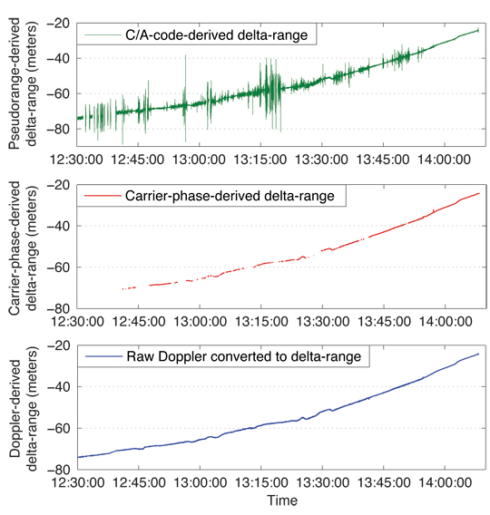
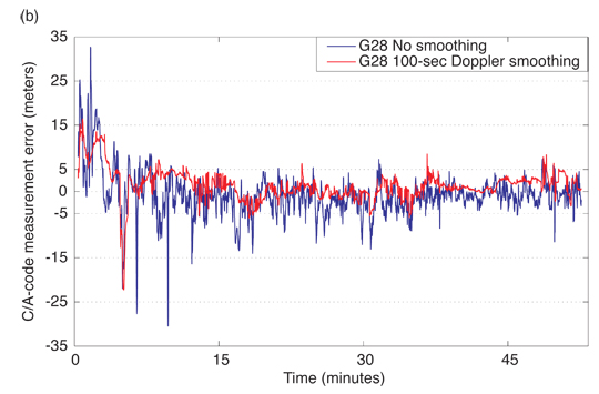
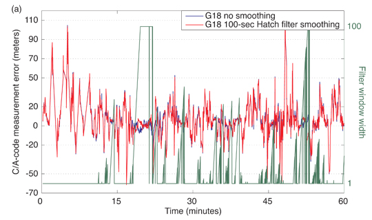
GPS and other global navigation satellite systems use the Doppler shift of the received carrier frequencies to determine the velocity of a moving receiver. Doppler-derived velocity is far more accurate than that obtained by simply differencing two position estimates. But GPS Doppler measurements can be used in other ways, too. In this month’s column, we look at how Doppler measurements can be used to smooth noisy code-based pseudoranges to improve the precision of autonomous positioning as well as to improve the availability of single-frequency real-time kinematic positioning, especially in urban environments.
Correction and Further Details
The first experimental Transit satellite was launched in 1959. A brief summary of subsequent launches follows:
Transit 1A launched 17 September 1959 failed to reach orbit
Transit 1B launched 13 April 1960 successfully
Transit 2A launched 22 June 1960 successfully
Transit 3A launched 30 November 1960 failed to reach orbit
Transit 3B launched 22 February 1961 failed to deploy in correct orbit
Transit 4A launched 29 June 1961 successfully
Transit 4B launched 15 November 1961 successfully
Transits 4A and 4B used the 150/400 MHz pair of frequencies and provided geodetically useful results.
A series of Transit prototype and research satellites was launched between 1962 and 1964 with the first fully operational satellite, Transit 5-BN-2, launched on 5 December 1963.
The first operational or Oscar-class Transit satellite, NNS O-1, was launched on 6 October 1964.
The last pair of Transit satellites, NNS O-25 and O-31, was launched on 25 August 1988.
“Innovation” is a regular column that features discussions about recent advances in GPS technology and its applications as well as the fundamentals of GPS positioning. The column is coordinated by Richard Langley of the Department of Geodesy and Geomatics Engineering at the University of New Brunswick, who welcomes your comments and topic ideas. To contact him, email lang @ unb.ca.
Real-time kinematic (RTK) techniques enable centimeter-level, relative positioning. The technology requires expensive, dedicated, dual-frequency, geodetic-quality receivers. However, myriad industrial and engineering applications would benefit from small-size, cost-effective, single-frequency, low-power, and high-accuracy RTK satellite positioning. Can such a sensor be developed and will it deliver? If feasible, such an instrument would find many applications within urban environments — but here the barriers to success are higher. In this article, we show how some of the problems can be overcome.
Single-Frequency RTK
Low-cost single-frequency (L1) GPS receivers have attained mass-market status in the consumer industry. Notwithstanding current levels of maturity in GPS hardware and algorithms, these receivers still suffer from large positioning errors. Any positioning accuracy improvement for mass-market receivers is of great practical importance, especially for many applications demanding small size, cost-effectiveness, low power consumption, and highly accurate GPS positioning and navigation. Examples include mobile mapping technology; machine control; agriculture fertilization and yield monitoring; forestry; utility services; intelligent transportation systems; civil engineering projects; unmanned aerial vehicles; automated continuous monitoring of landslides, avalanches, ground subsidence, and river level; and monitoring deformation of built structures. Moreover, today an ever-increasing number of smartphones and handsets come equipped with a GPS receiver. In those devices, the increasing sophistication of end-user applications and refinement of map databases are continually tightening the accuracy requirements for GPS positioning.
For single-frequency users, the RTK method does appear to offer the promise of highly precise position estimates for stationary and moving receivers and can even be considered a candidate for integration within mobile handhelds. Moreover, the RTK approach is attractive because the potential of the existing national infrastructures such as Great Britain’s Ordnance Survey National GNSS Network-RTK (OSNet) infrastructure, as well as enabling technologies such as the Internet and the cellular networks, can be exploited to deliver RTK corrections and provide high-precision positioning and navigation.
The basic premise of relative (differential) positioning techniques such as RTK is that many of the sources of GNSS measurement errors including the frequency-dependent error (the ionospheric delay) are spatially correlated. By performing relative positioning between receivers, the correlated measurement errors are completely cancelled or greatly reduced, resulting in a significant increase in the positioning accuracy and precision.
Single-Frequency Challenges. Although RTK positioning is a well-established and routine technology, its effective implementation for low-cost, single-frequency L1 receivers poses many serious challenges, especially in difficult and degraded signal environments for GNSS such as urban canyons. The most serious challenge is the use of only the L1 frequency for carrier-phase integer ambiguity resolution and validation. Unfortunately, users with single-frequency capability do not have frequency diversity and many options in forming useful functions and combinations for pseudorange and carrier-phase observables. Moreover, observations from a single-frequency, low-cost receiver are typically “biased” due to the high level of multipath and/or receiver signal-tracking anomalies and also the low-cost patch antenna design that is typically used. In addition, in those receivers, measurements are typically contaminated with high levels of noise due to the low-cost hardware design compared to the high-end receivers. This makes the reliable fixing of the phase ambiguities to their correct integer values, for single-frequency users, a non-trivial problem. As a consequence, the reliability of single-frequency observations to resolve ambiguities on the fly in an operational environ
ment is relatively low compared to the use of dual-frequency observations from geodetic-quality receivers. Improving performance will be difficult, unless high-level noise and multipath can be dealt with effectively or unless ambiguity resolution techniques can be devised that are more robust and are less sensitive to the presence of biases and/or high levels of noise in the observations.
Traditionally, single-frequency RTK positioning requires long uninterrupted initialization times to obtain reliable results, and hence have a time-to-fix ambiguities constraint. Times of 10 to 25 minutes are common. Observations made at tens of continuous epochs are used to determine reliable estimates of the integer phase ambiguities. In addition, these continuous epochs must be free from cycle slips, loss of lock, and interruptions to the carrier-phase signals for enough satellites in view during the ambiguity fixing procedure. Otherwise, the ambiguity resolution will fail to fix the phase ambiguities to correct integer values. To overcome these drawbacks and be able to determine the integer phase ambiguities and thus the precise relative positions, observations made at only one epoch (single-epoch) can be used in resolving the integer phase ambiguities. This allows instantaneous RTK positioning and navigation for single-frequency users such that the problem of cycle slips, discontinuities, and loss of lock is eliminated. However, for single-frequency users, the fixing of the phase ambiguities to their correct integer values using a single epoch of observations is a non-trivial problem; indeed, it is considered the most challenging scenario for ambiguity resolution at the present time.
Instantaneous RTK positioning relies fundamentally upon the inversion of both carrier-phase measurements and code measurements (pseudoranges) and successful instantaneous ambiguity resolution. However, in this approach, the probability of fixing ambiguities to correct integer values is dominated by the relatively imprecise pseudorange measurements. This is more severe in urban areas and difficult environments where the level of noise and multipath on pseudoranges is high. This problem may be overcome partially by carrier smoothing of pseudoranges in the range/measurement domain using, for example, the Hatch filter. While carrier-phase tracking is continuous and free from cycle slips, the carrier smoothing of pseudoranges with an optimal smoothing filter window-width can effectively suppress receiver noise and short-term multipath noise on pseudoranges. However, the effectiveness of the conventional range-domain carrier-smoothing filters is limited in urban areas and difficult GNSS environments because carrier-phase measurements deteriorate easily and substantially due to blockages and foliage and suffer from phase discontinuities, cycle-slip contamination, and other measurement anomalies. This is illustrated in Figure 1. The figure shows that in a kinematic urban environment, frequent carrier-phase outages and anomalies occur, which cause frequent resets of the carrier-smoothing filter and hence carrier smoothing of pseudoranges suffers in robustness and effective continuous smoothing.
Figure 1. Satellite tracking and carrier-phase anomaly summary during the observation time-span. These data were collected in a dense urban environment in both static and kinematic mode. The superimposed red-points show epochs where carrier-phase observables are either missing or contaminated with cycle slips, loss of locks, and/or other measurement anomalies.
Doppler Frequency Shift. While carrier-phase tracking can be discontinuous in the presence of continuous pseudoranges, a receiver generates continuous Doppler-frequency-shift measurements. The Doppler measurements are immune to cycle slips. Moreover, the precision of the Doppler measurements is better than the precision of pseudoranges because the absolute multipath error of the Doppler observable is only a few centimeters. Thus, devising methods that utilize the precision of raw Doppler measurements to reduce the receiver noise and high-frequency multipath on pseudoranges may prove valuable especially in GNSS-challenged environments. Figure 2 shows an example of the availability and the precision of the receiver-generated Doppler measurements alongside the delta-range values derived from the C/A-code pseudoranges and from the L1 carrier-phase measurements. This figure also shows that frequent carrier-phase outages and anomalies occur while for every C/A-code pseudorange measurement there is a corresponding Doppler measurement available.
Figure 2. Plots of C/A-code-pseudorange-derived delta-ranges (top), L1 carrier-phase-derived delta-ranges (middle), and L1 raw receiver-generated Doppler shifts that are transformed into delta-ranges for the satellite PRN G18 during the observation time-span when it was tracked by the receiver (bottom).
Smoothing. A rich body of literature has been published exploring aspects of carrier smoothing of pseudoranges. One factor that has not received sufficient study in the literature is utilization of Doppler measurements to smooth pseudoranges and to investigate the influence of improved pseudorange accuracy on both positioning and the integer-ambiguity resolution. Utilizing the Doppler measurements to smooth pseudoranges could be a good example of an algorithm that maximally utilizes the information redundancy and diversity provided by a GPS/GNSS receiver to improve positioning accuracy. Moreover, utilizing the Doppler measurements does not require any hardware modifications to the receiver. In fact, receivers measure Doppler frequency shifts all the time as a by-product of satellite tracking.
GNSS Doppler Measurement Overview
The Doppler effect is the apparent change in the transmission frequency of the received signal and is experienced whenever there is any relative motion between the emitter and receiver of wave signals. Theoretically, the observed Doppler frequency shift, under Einstein’s Special Theory of Relativity, is approximately equal to the difference between the received and transmitted signal frequencies, which is approximately proportional to the receiver-satellite topocentric range rate.
Beat Frequency. However, the transmitted frequency is replicated locally in a GNSS receiver. Therefore, strictly speaking, the difference of the received frequency and the receiver locally generated replica of the transmitted frequency is the Doppler frequency shift that is also termed the beat frequency. If the receiver oscillator frequency is the same as the satellite oscillator frequency, the beat frequency represents the Doppler frequency shift due to the relative, line-of-sight motion between the satellite and the receiver. However, the receiver internal oscillator is far from being perfect and therefore, the receiver Doppler measurement output is the apparent Doppler frequency shift (that includes local oscillator effects). The Doppler frequency shift is also subject to satellite-oscillator frequency bias and other disturbing effects such as atmospheric effects on the signal propagation.
To estimate the range rate, a receiver typically forms an average of the delta-range by simply integrating the Doppler over a very short period of time (for example, 0.1 second) and then dividing it by the duration of the integration interval. Since the integration of frequency over time gives the phase of the signal over that time interval, the procedure continuously forms the carrier-phase observable that is the integrated Doppler over time. Therefore, Doppler frequency shift can also be estimated by time differencing carrier-phase measurements. The carrier-phase-derived Doppler is com
puted over a longer time span, leading to smoother Doppler measurements, whereas direct loop filter output is an instantaneous measure produced over a short time interval.
Doppler frequency shift is routinely used to determine the satellite or user velocity vector. Apart from velocity determination, it is worth mentioning that Doppler frequency shifts are also exploited for coarse GPS positioning. Moreover, the user velocity vector obtained from the raw Doppler frequency shift can be and has been applied by a number of researchers to instantaneous RTK applications to constrain the float solution and hence improve the integer-ambiguity-resolution success rates in kinematic surveying. In this article, a simple combination procedure of the noisy pseudorange measurements and the receiver-generated Doppler measurements is suggested and its benefits are examined.
Doppler-Smoothing Algorithm Description
Motivated both by the continual availability and the centimeter-level precision of receiver-generated (raw) Doppler measurements, even in urban canyons, a method has been introduced by the authors that utilizes the precision of raw Doppler measurements to reduce the receiver noise and high-frequency multipath on code pseudoranges. For more detail on the Doppler-smoothing technique, see Further Reading. The objective is to smooth the pseudoranges and push the accuracy of the code-based or both code- and carrier-based positioning applications in GNSS-challenged environments.
Previous work on Doppler-aided velocity/position algorithms is mainly in the position domain. In those approaches, the improvement in the quality of positioning is gained mainly by integrating the kinematic velocities and accelerations derived from the Doppler measurement in a loosely coupled extended Kalman filter or its variations such as the complementary Kalman filter. Essentially, these techniques utilize the well-known ability of the Kalman filter to use independent velocity estimates to reduce the noise of positioning solutions and improve positioning accuracy. The main difference among these position-domain filters is that different receiver dynamic models are used.
The proposed method combines centimeter-level precision receiver-generated Doppler measurements with pseudorange measurements in a combined pseudorange measurement that retains the significant information content of each.
Two-Stage Process. The proposed Doppler-smoothing process has two stages: (1) the prediction or initialization stage and (2) the filtering stage. In the prediction stage, a new estimated smoothed value of the pseudorange measurement for the Doppler-smoothing starting epoch is obtained. In this stage, for a fixed number of epochs, a set of estimated pseudoranges for the starting epoch is obtained from the subsequent pseudorange and Doppler measurements. The estimated pseudoranges are then averaged to obtain a good estimated starting point for the smoothing process. The number of epochs used in the prediction stage is the averaging window-width or Doppler-smoothing-filter length. In the filtering stage, the smoothed pseudorange profile is constructed using the estimated smoothed starting pseudorange and the integrated Doppler measurements over time. The Doppler-smoothing procedures outlined here can be performed successively epoch-by-epoch (that is, in a moving filter), where the estimated initial pseudorange (the averaged pseudorange) is updated from epoch to epoch. Alternatively, an efficient and elegant implementation of the measurement-domain Doppler-smoothing method is in terms of a Kalman filter, where it can run as a continuous process in the receiver from the first epoch (or in post-processing software, but then without the real-time advantage). This filter allows real-time operation of the Doppler-smoothing approach.
In the experiments described in this article, a short filter window-width is used. The larger the window width used in the averaging filter process, the more precise the averaged pseudorange becomes. However, this filter is also susceptible to the ionospheric divergence phenomenon because of the opposite signs of the ionospheric contribution in the pseudorange and Doppler observables. Therefore, the ionospheric divergence effect between pseudoranges and Doppler observables increases with averaging window-width and the introduced bias in the averaged pseudoranges become apparent for longer filter lengths.
Using the propagation of variance law, it can be shown that the precision of the delta-range calculated with the integrated Doppler measurements over time depends on both the Doppler-measurement epoch interval and the precision of the Doppler measurements, assuming that noise/errors on the measurements are uncorrelated.
Experimental Results
To validate the improvement in the performance and availability of single-frequency instantaneous RTK in urban areas, the proposed Doppler-aided instantaneous RTK technique has been investigated using actual GPS data collected in both static and kinematic pedestrian trials in central London. In this article, we only focus on the static results and the kinematic trial results are omitted. It is remarked, however, that the data collected in the static mode were post-processed in an epoch-by-epoch approach to simulate RTK processing.
In the static testing, GPS test data were collected with a measurement rate of 1 Hz. At the rover station, a consumer-grade receiver with a patch antenna was used. This is a single-frequency 16-channel receiver that, in addition to the C/A-code pseudoranges, is capable of logging carrier-phase measurements and raw Doppler measurements. Reference station data were obtained from the Ordnance Survey continuously operating GNSS network. Three nearby reference stations were selected that give different baseline lengths: Amersham (AMER) ≈ 38.3 kilometers away, Teddington (TEDD) ≈ 20.8 kilometers away, and Stratford (STRA) ≈ 7.1 kilometers away. In addition, a virtual reference station (VRS) was also generated in the vicinity (60 meters away) of the rover receiver.
Doppler-Smoothing. Before we present the improvement in the performance of instantaneous RTK positioning, the effect of the Doppler-smoothing of the pseudoranges in the measurement domain and comparison with carrier-phase smoothing of pseudoranges is given. To do this, we computed the C/A-code measurement errors or observed range deviations (the differences between the expected and measured pseudoranges) in the static mode (with surveyed known coordinates) using raw, Doppler-smoothed and carrier-smoothed pseudoranges. FIGURE 3a illustrates the effect of 100-second Hatch-filter carrier smoothing and FIGURE 3b shows a 100-second Doppler-smoothing of the pseudoranges for satellite PRN G28 (RINEX satellite designator) with medium-to-high elevation angle. The raw observed pseudorange deviations (in blue) are also given as reference. The quasi-sinusoidal oscillations are characteristic of multipath. Comparing the Doppler-smoothing in Figure 3b to the Hatch carrier-smoothing in Figure 3a, it can be seen that Doppler-smoothing of pseudoranges offers a modest improvement and is more robust and effective than that of the traditional Hatch filter in difficult environments.
Figure 3. Smoothed pseudorange errors (observed range deviations) using the traditional Hatch carrier-smoothing filter. Smoothing filter length in the experiments for both filters was set to 100 seconds. Satellite PRN G28 was chosen to represent a satellite at medium-to-high elevation angle.Figure 3. Smoothed pseudorange errors (observed range deviations) using the Doppler-smoothing filter. Smoothing filter length in the experiments for both filters was set to 100 seconds. Satellite PRN G28 was chosen to represent a satellite at medium-to-high elevation angle.
Figure 4a illustrates carrier-phase Hatch-filter smoothing for low-elevation angle satellite PRN G18. In this figure, the Hatch carrier-smoothing filter reset is indicated. It can be seen that due to the frequent carrier-phase discontinuities and cycle slips, the smoothing has to be reset and restarted from the beginning and hardly reaches its full potential. In contrast, Doppler smoothing for PRN G18 shown in FIGURE 4b had few filter resets and managed effectively to smooth the very noisy pseudorange in some sections of the data.
Figure 4. Smoothed pseudorange errors (observed range deviations) and filter resets and filter length (window width) using the traditional Hatch carrier-smoothing filter. Smoothing filter length in the experiments for both filters was set to 100 seconds. Satellite PRN G18 was chosen to represent a satellite at low elevation angle as it rises from 10 to 30 degrees.Figure 4. Smoothed pseudorange errors (observed range deviations) and filter resets and filter length (window width) using the Doppler-smoothing. Smoothing filter length in the experiments for both filters was set to 100 seconds. Satellite PRN G18 was chosen to represent a satellite at low elevation angle as it rises from 10 to 30 degrees.
Considering RTK in this analysis, we can demonstrate the increase in the success rate of the Doppler-aided integer ambiguity resolution (and hence the RTK availability) by comparison of the obtained integer ambiguity vectors from the conventional LAMBDA (Least-squares AMBiguity Decorrelation Adjustment) ambiguity resolution method using Doppler-smoothed pseudoranges with those obtained without Doppler-aiding in post-processed mode. The performance of ambiguity resolution was evaluated based on the number of epochs where the ambiguity validation passed the discrimination/ratio test. The ambiguity validation ratio test was set to the fixed critical threshold of 2.5 in all the experiments. In addition to the ratio test, the fixed solutions obtained using the fixed integer ambiguity vectors that passed the ratio test were compared against the true position of the surveyed point to make sure that indeed the correct set of integer ambiguities were estimated.
The overall performance of the single-epoch single-frequency integer ambiguity resolution obtained by the conventional LAMBDA ambiguity resolution method without Doppler-aiding is shown in Figure 5 for baselines from 60 meters up to 38 kilometers in length. In comparison, the performance of the single-epoch single-frequency integer ambiguity resolution from the LAMBDA method using Doppler-smoothed pseudoranges are shown in Figure 6 for those baselines and they are compared with integer ambiguity resolution success rates of the conventional LAMBDA ambiguity resolution method without Doppler-aiding. Figure 6 shows that using Doppler-smoothed pseudoranges enhances the probability of identifying the correct set of integer ambiguities and hence increases the success rate of the integer ambiguity resolution process in instantaneous RTK, providing higher availability. This is more evident for shorter baselines. For long baselines, the residual of satellite-ephemeris error and atmospheric-delay residuals that do not cancel in double differencing potentially limits the effectiveness of the Doppler-smoothing approach. It is well understood that those residuals for long baselines strongly degrade the performance of ambiguity resolution. Relative kinematic positioning with single frequency mass-market receivers in urban areas using VRS has also shown improvement.
Figure 5. Single-epoch single-frequency integer ambiguity resolution success rate obtained by the conventional LAMBDA ambiguity resolution method without Doppler-aiding.Figure 6. Plots of integer ambiguity resolution success rates: single-epoch single-frequency integer ambiguity resolution success rate obtained by the conventional LAMBDA ambiguity resolution method without Doppler-aiding (in blue) and using Doppler-smoothed pseudoranges (in green).
Conclusion
In urban areas, the proposed Doppler-smoothing technique is more robust and effective than traditional carrier smoothing of pseudoranges. Static and kinematic trials confirm this technique improves the accuracy of the pseudorange-based absolute and relative positioning in urban areas characteristically by the order of 40 to 50 percent.
Doppler-smoothed pseudoranges are then used to aid the integer ambiguity resolution process to enhance the probability of identifying the correct set of integer ambiguities. This approach shows modest improvement in the ambiguity resolution success rate in instantaneous RTK where the probability of fixing ambiguities to correct integer values is dominated by the relatively imprecise pseudorange measurements.
The importance of resolving the integer ambiguities correctly must be emphasized. Therefore, devising innovative and robust methods to maximize the success rate and hence reliability and availability of single-frequency, single-epoch integer ambiguity resolution in the presence of biased and noisy observations is of great practical importance especially in GNSS-challenged environments.
Acknowledgments
The study reported in this article was funded through a United Kingdom Engineering and Physical Sciences Research Council Engineering Doctorate studentship in collaboration with the Ordnance Survey. M. Bahrami would like to thank his industrial supervisor Chris Phillips from the Ordnance Survey for his continuous encouragement and support. Professor Paul Cross is acknowledged for his valuable comments. The Ordnance Survey is acknowledged for sponsoring the project and providing detailed GIS data.
Manufacturer
The data for the trial discussed in this article were obtained from a u-blox AG AEK-4T receiver with a u-blox ANN-MS-0-005 patch antenna.
Mojtaba Bahrami is a research fellow in the Space Geodesy and Navigation Laboratory (SGNL) at University College London (UCL). He holds an engineering doctorate in space geodesy and navigation from UCL.
Marek Ziebart is a professor of space geodesy at UCL. He is the director of SGNL and vice dean for research in the Faculty of Engineering Sciences at UCL.
FURTHER READING
• Carrier Smoothing of Pseudoranges
“Optimal Hatch Filter with an Adaptive Smoothing Window Width” by B. Park, K. Sohn, and C. Kee in Journal of Navigation, Vol. 61, 2008, pp. 435–454, doi: 10.1017/S0373463308004694.
“Optimal Recursive Least-Squares Filtering of GPS Pseudorange Measurements” by A. Q. Le and P. J. G. Teunissen in VI Hotine-Marussi Symposium on Theoretical and Computational Geodesy, Wuhan, China, May 29 – June 2, 2006, Vol. 132 of the International Association of Geodesy Symposia, Springer-Verlag, Berlin and Heidelberg, 2008, Part II, pp. 166–172, doi: 10.1007/978-3-540-74584-6_26.
“The Synergism of GPS Code and Carrier Measurements” by R. Hatch in Proceedings of the 3rdInternational Geodetic Symposium on Satellite Doppler Positioning, Las Cruces, New Mexico, February 8-12, 1982, Vol. 2, pp. 1213–1231.
• Combining Pseudoranges and Carrier-phase Measurements in the Position Domain
“Position Domain Filtering and Range Domain Filtering for Carrier-smoothed-code DGNSS: An Analytical Comparison” by H. Lee, C. Rizos, and G.-I. Jee in IEE Proceedings Radar, Sonar and Navigation, Vol. 152, No. 4, August 2005, pp. 271–276, doi:10.1049/ip-rsn:20059008.
“Complementary Kalman Filter for Smoothing GPS Position with GPS Velocity” by H. Leppakoski, J. Syrjarinne, and J. Takala in Proceedings of ION GPS/GNSS 2003, the 16th International Technical Meeting of the Satellite Division of The Institute of Navigation, Portland, Oregon, September 9–
12, 2003, pp. 1201–1210.
“GPS Navigation: Combining Pseudorange with Continuous Carrier Phase Using a Kalman Filter” by P. Y. C. Hwang and R. G. Brown in Navigation, Journal of The Institute of Navigation, Vol. 37, No. 2, 1990, pp. 181–196.
• Doppler-derived Velocity Information and RTK Positioning
“Advantage of Velocity Measurements on Instantaneous RTK Positioning” by N. Kubo in GPS Solutions, Vol. 13, No. 4, 2009, pp. 271–280, doi: 10.1007/s10291-009-0120-9.
• Doppler Smoothing of Pseudoranges and RTK Positioning
Doppler-Aided Single-Frequency Real-Time Kinematic Satellite Positioning in the Urban Environment by M. Bahrami, Ph.D. dissertation, Space Geodesy and Navigation Laboratory, University College London, U.K., 2011.
“Instantaneous Doppler-Aided RTK Positioning with Single Frequency Receivers” by M. Bahrami and M. Ziebart in Proceedings of PLANS 2010, IEEE/ION Position Location and Navigation Symposium, Indian Wells, California, May 4–6, 2010, pp. 70–78, doi: 10.1109/PLANS.2010.5507202.
“Getting Back on the Sidewalk: Doppler-Aided Autonomous Positioning with Single-Frequency Mass Market Receivers in Urban Areas” by M. Bahrami in Proceedings of ION GNSS 2009, the 22nd International Technical Meeting of the Satellite Division of The Institute of Navigation, Savannah, Georgia, 22–25 September 2009, pp. 1716–1725.
• Integer Ambiguity Resolution
“GPS Ambiguity Resolution and Validation: Methodologies, Trends and Issues” by D. Kim and R. B. Langley in Proceedings of the 7th GNSS Workshop – International Symposium on GPS/GNSS, Seoul, Korea, 30 November – 2 December 2000, Tutorial/Domestic Session, pp. 213–221.
“The Least-Squares Ambiguity Decorrelation Adjustment: a Method for Fast GPS Integer Ambiguity Estimation” by P.J.G. Teunissen in Journal of Geodesy, Vol. 70, No. 1–2, 1995, pp. 65–82, doi: 10.1007/BF00863419.
Plus: GLONASS CDMA Tracked, Third Beidou-2 Launched
The second report from non‐governmental members of the LightSquared/GPS Technical Working Group (TWG) was filed with the Federal Communications Commission (FCC) on April 15. For those anxious to see actual results of interference/desensitization of GPS receivers by the proposed LightSquared terrestrial signal — or, conversely, absence of said results — the report does not contain any such hard news. It relates the set-up of TWG work sub-teams to test various categories of GPS devices and receivers.
The sub-teams have identified laboratories for testing activities, developed test plans, and identified devices, receivers, and systems to be tested. Attachments to the report include current draft test plans and the current list of devices and receiver models submitted for testing by companies.
The following sections summarize the testing laboratories and devices selected for testing by each sub-team:
aviation
cellular
general location/navigation
high precision, networks, and timing. These three sub-teams are collaborating to a large extent.
space-based receivers.
The full report also includes a “high-level description of test plan” by each sub-team.
Aviation Sub‐Team. The aviation sub‐team will rely primarily on testing, funded by the Federal Aviation Administration (FAA), that will be performed at Zeta Associates Incorporated of Fairfax, Virginia.
Additional testing is planned by the U.S. government at White Sands Missile Range and Holloman Air Force Base, both in New Mexico, for use by the National PNT Engineering Forum (NPEF) LightSquared Working Group. These results will be considered for inclusion in the TWG Final Report by the aviation sub‐team. Presumably, this group will test military receivers, under classified categorization.
The aviation receivers are representative of those in use today. Their selection was based mainly upon device availability (those already owned by the FAA Technical Center). They are: Canadian Marconi GLSSU 5024; Garmin 300XL; Garmin GNS 430W; Garmin GNS 480; Rockwell Collins GLU‐920 multimode receiver; Rockwell Collins GLU‐925 multimode receiver; Rockwell Collins GNLU‐930 multimode receiver; Symmetricomm timing card (used for an FAA automation system); WAAS NovAtel G‐II ground reference station; and Zyfer timing receiver (used for the WAAS ground network).
Cellular Sub‐Team. The cellular sub‐team is in the process of engaging PC TEST, Columbia, Maryland; CETECOM, Milpitas, California; InterTek, Lexington, Kentucky; and ETS Lindgren, Cedar Park, Texas, for device testing.
The cellular sub‐team expects to test approximately 50 different device models. The selections represent current and legacy devices and have been prioritized based on sales volumes. While it is expected that there will be some representation of data‐only devices and femtocells, the testing will focus largely on handheld devices.
Those designated for testing are: Apple iPhone 4 (GSM and CDMA); HTC A6366; HTC ADR6200; HTC ADR63002; HTC ADR63003; HTC ADR6400L; HTC Touch Pro 2; LG Lotus Elite; LG Rumor Touch; LG VN250; LG VS740; LG VX5500; LG VX5600; LG VX8300; LG VX8360; LG VX8575; LG VX9100; LG VX9200; Motorola A855; Motorola DROID X; Motorola VA76R; Motorola W755; Nokia 6650; Nokia E71x; RIM 8330C; RIM 8530; RIM 9630; RIM 9650; RIM 9800; Samsung Moment; Samsung SCH‐U310; Samsung SCH‐U350; Samsung SCH‐U450; Samsung SCH‐U640; Samsung SCH‐U750; Samsung SGHi617; Samsung SGHi917; Sierra Wireless 250 U USG 3G/4G; and Sony Ericsson W760a.
General Location/Navigation. This sub-team has chosen Alcatel/Lucent as its initial facility for testing. Twenty-six devices were selected based on nominations by manufacturers represented on the sub‐team, considering the percentage of the installed user base.
They include: Garmin Forerunner 110 and 305; Garmin ETREX‐H; Garmin Dakota 20; Garmin Oregon 550; Garmin GTU 10; BI Inc. ExacuTrack One; Garmin GPS 17X; Garmin GPSMAP 441; Hemisphere Vector MV101; GM OnStar (model TBD); Garmin GVN 54; TomTom XL335; TomTom ONE 3RD Edition; TomTom GO 2505; Garmin nűvi 2X5W, 13XX, 3XX, and 37XX; Garmin GPSMAP 496; Garmin aera 5xx; Honeywell Bendix/King AV8OR; Trimble iLM2730; Trimble TVG‐850; Trimble Placer Gold; and Hemisphere Outback S3.
High Precision-Networks-Timing. The HPN&T sub‐teams are collaborating extensively to develop joint test plans and procedures. The joint sub-teams have chosen the U.S. Navy’s NAVAIR facility for testing.
To be tested are: Hemisphere R320; Hemisphere A320; Deere iTC; Deere SF‐3000; Deere SF‐3050; Trimble MS990; Trimble MS992; Trimble AgGPS 252, AgGPS 262, AgGPS 442, and AgGPS EZguide 500; Trimble CFX 750; Trimble FMX; Trimble GeoExplorer 3000 series GeoXH and GeoXT; Trimble GeoExplorer 6000 series GeoXH and GeoXT; Trimble Juno SB; Trimble NetR9 and NetR5; Trimble R8 GNSS; Trimble 5800; Leica SR530; Leica GX1200 Classic; Leica GX1230GG; Leica GR10; Leica Uno; Leica GS15; Topcon HiPer Ga and HiPer II; Topcon GR‐3 and GR‐5; Topcon MC‐R3; Topcon NET‐G3A; Topcon TruPath/AGI‐3; NovAtel PROPAK‐G2‐Plus; NovAtel FLEXG2‐STAR; NovAtel FLEXPAK‐G2‐V1, FLEXPAK‐G2‐V2 and FLEXPAK6; NovAtel PROPAK‐V3; NovAtel DL‐V3; Septentrio PolaRx3e; and Septentrio AsteRx3.
Space‐Based Receivers. Lab testing has been conducted at the NASA Jet Propulsion Laboratory (JPL) in California. The receivers are used by NASA for space‐based missions and high-precision science applications. The TWG agreed that these would be tested at JPL by NASA, with participation by LightSquared personnel, and the results provided to the TWG; see Appendix G
The devices tested are current or representative of GPS receivers in use by NASA or planned for use in the near future for space and science applications: TriG (NASA Next‐generation Space Receiver) and IGOR (Space Receiver).
NASA/JPL also tested the following high-precision receivers and shared the results with the HPT&N sub‐team: JAVAD Delta G3T (High Precision‐IGS) and Ashtech Z12 (High Precision‐IGS).
Conclusion. For all sub-teams, analyses will consider both LightSquared’s expected transmit power of 62 dBm per channel and its maximum authorized transmit power of 72 dBm per channel.
The WG co‐chairs will update the Commission on its progress in a subsequent report on May 16.
The April 15 TWG report contains these appendices: Working Group Roster; List of Receivers and Devices; Aviation Test Procedure; Cellular Test Plan Draft; General Location/Navigation Test Plan Draft; High Precision/Networks/Timing Test Plans Draft; Space‐Based Receivers Test Process.
GLONASS CDMA: New Era’s Dawn Glimpsed from Multiple Receivers
The newest Russian satellite, launched on February 26, began transmitting its new code-division multiple-access (CDMA) signal on April 7. In a clear break from all previous GLONASS signals, which are frequency-division multiple-access (FDMA), the new signal is expressly designed to be interoperable with current and future GPS signals, and with the coming Galileo signals, all of which have a CDMA structure. Thus, a new era of GNSS, truly global navigation satellite systems, began on April 7.
JAVAD GNSS was the first company to announce that it had tracked CDMA signals of the GLONASS-K satellite in
the L3 GLONASS band. Data was logged at the company’s Moscow office on April 8 from 02:30 until 07:30 UTC. The satellite’s pseudorange (in chips) and signal-to-noise ratio (in relative numbers) are shown in Figures 1 and 2.
Figure 1. GLONASS-K’s pseudorange in chips, courtesy of JAVAD GNSS. The y-axis goes from 0 to 12,000 in increments of 2,000; the x-axis goes from 0 to 500 in increments of 100. (Click to enlarge.)Figure 2. GLONASS-K’s signal-to-noise ratio (in relative numbers), courtesy of JAVAD GNSS. The y-axis goes from 0 to 10,000 in increments of 2,000; the x-axis goes from 0 to 500 in increments of 100. (Click to enlarge.)
On April 11, the satellite’s code-minus-phase and signal-to-noise ratio were tracked (Figures 3 and 4). Data quality is quite similar to GPS, according to the company.
Figure 3. GLONASS-K satellite’s code-minus-phase data (courtesy of JAVAD GNSS). (Click to enlarge.)Figure 4. GLONASS-K satellite’s signal-to-noise ratio (courtesy of JAVAD GNSS). (Click to enlarge.)
Future GLONASS satellites of the K1 and subsequent K2 generations will broadcast CDMA signals in multiple frequency bands. GLONASS-K satellites are markedly different from their predecessors. They are lighter, use an unpressurized housing (similar to that of GPS satellites), have improved clock stability, and a longer, 10-year design life. There will be two versions: GLONASS-K1 will transmit a CDMA signal on a new L3 frequency, and GLONASS-K2 will in addition feature CDMA signals on L1 and L2 frequencies. The CDMA signal in the L3 band has a center frequency of 1202.025 MHz.
The new generations of GLONASS signals and satellites are described in detail in the April “Innovation” column of GPS World, edited by Richard Langley.
Septentrio Navigation of Leuven, Belgium, also tracked GLONASS CDMA L3 signal with its AsteRx3 receivers. Figure 5 shows the C/N0 in dB-Hz of the legacy L1-C/A signal and of the data component of the new L3 CDMA signal. The graph covers the time span starting at 20:30 (UTC) on April 10 and ending at 02:00 on April 11. Figure 6 shows the de-trended code minus phase from L1-C/A and L3 signals. Such a plot provides a glimpse of the code measurement multipath and noise, according to the company.
Figure 5. GLONASS-K1 AsteRx3 measurements; C/N0 in dB-Hz of L1-C/A and L3 CDMA (courtesy of Septentrio Navigation).Figure 6. GLONASS-K1 AsteRx3 measurements; de-trended code minus phase of L1-C/A and L3 CDMA (courtesy of Septentrio Navigation).
Topcon Positioning Systems (TPS) also released data on the new signal, stating that signals from the new satellite “provide an additional accuracy advantage over older satellites.” Figures 7 and 8 show data from the company’s Moscow office.
Figure 7. Pseudorange-phase of four signals transmitted by the new K1 satellite (courtesy of Topcon Positioning Systems). (Click to enlarge.) Figure 8. Signal-to-noise ratios of four signals transmitted by the new K1 satellite (courtesy of Topcon Positioning Systems). (Click to enlarge.)
Finally, the German Aerospace Center’s Institute of Communications and Navigation recorded the spectrum of the GLONASS CDMA signal, captured with a 25-meter dish antenna, Raisting Satellite Earth Station, near Munich.
The signal spectrum spans at least 40 MHz (Figure 9). It contains additional sidelobes not shown in the plot. The plot indicates total power of all components of the transmitted signal.
Figure 9. GLONASS CDMA signal’s power over frequency (courtesy of the German Space Agency, DLR).
Third Beidou-2 IGSO Launched
China’s BeiDou-2 (Compass) satellite launched on April 9 has attained a circularized orbit, joining two inclined geosynchronous orbit (IGSO) satellites to form a mini-constellation centered on an east longitude of about 120 degrees. While BeiDou-IGSO-3’s orbit might still be tweaked slightly, it is clear that the orbits of the three satellites are arranged so that there will always be one satellite with a high elevation angle over China, according to the CANSPACE news service operated by the University of New Brunswick.
The latest spacecraft joins four geostationary satellites, a middle-Earth orbiting vehicle, and the two other IGSO satellites now on orbit. As the first Chinese launch in 2011, the new arrival presages much activity to come. With eight now flying, six more spacecraft are scheduled to rise by 2012, completing a 14-satellite constellation to provide a regional service over eastern Asia. The regional system will consist of five geostationary or GEO, five IGSO, and four medium-Earth orbit satellites.
Long-range plans envision a 35-satellite constellation providing global service by 2020: 27 MEOs, 5 GEO satellites, and 3 IGSOs. The satellites will transmit signals on the 1195.14–1219.14 MHz, 1256.52–1280.52 MHz, 1559.05–1563.15 MHz, and 1587.69-1591.79 MHz carrier frequencies.
Compass satellites have an announced lifespan of eight years.
Three IGSO satellite tracks over China (image courtesy of CANSPACE).
By Thomas A. Stansell, Kenneth W. Hudnut, and Richard G. Keegan
The new GPS L1C signal will be broadcast by the Block III satellites, with first launches as early as 2014. L1C innovations significantly enhance PNT performance as well as interoperability with other GNSS signals. The authors describe the benefits of its new features and how best to make use of each one.
A highly evolved racehorse of a signal with outstanding technical performance, L1C was designed to significantly improve autonomous navigation, and to be interoperable with L1 signals from other GNSS providers. Its structure evolved from the earliest GPS signals: it shares with the C/A signal the L1 center frequency of 1575.42 MHz, coherence between the carrier frequency, the code clock rates, and the data rate, and the provision of a navigation data message.
L1C inherited significant improvements from subsequent developments, specifically WAAS, L5, and L2C. WAAS was the first GPS-related signal to use forward error correction (FEC) for its data. L5 was the first open signal design to use longer spreading codes (10,230 chips), to have separate data and data-less (pilot carrier) signal components, to employ an improved navigation message structure (CNAV), and to employ overlay codes to achieve a longer equivalent code length, improve correlation performance, and eliminate the need for bit synchronization. The L2C signal adopted most of these improvements but, instead of an overlay, substituted a much longer pilot carrier spreading code, not only to optimize correlation performance but also to decrease the number of time ambiguities after tracking the spreading codes.
The L1C signal design is amazing, not only because of its highly evolved and outstanding technical performance but also because a committee designed this racehorse of a signal rather than it becoming a camel. Table 1 lists key members of the L1C technical committee in alphabetical order. The list has two groups, technical contributors and government chairpersons. When each new signal aspect is introduced, the key contributor or contributors from this list will be identified.
Table 1. Key L1C contributors.
L1C is intended to be interoperable with L1 signals from other GNSS providers. To identify its signal type, we note that Galileo officials have identified three types of services, “open”, “commercial”, and “publicly regulated”. An open service is freely available to all users. A commercial service is limited to users who pay a fee to access the signal, which otherwise is denied by encryption. A publicly regulated service (PRS) also is encrypted but intended only for public safety applications. GPS is adopting the open service definition but will continue to distinguish encrypted signals as “military” because there are no encrypted commercial GPS services. L1C will be a new GPS open service signal, joining L1 C/A, L2C, and L5.
Although the term “civil signal” often is used, there can be confusion about its meaning. Within the U.S. government it is common to use the word “civil” to mean civil government agencies, e.g., the Department of Transportation (DOT). However, it’s clear the GPS C/A, L2C, L5, and L1C signals are “open” and intended for use by anyone. Therefore, we will use the term “civilian” or “open” in order not to imply that any of these signals is restricted in its use.
L1C Signal Development
The L1C signal structure has evolved from the earliest GPS signals first launched in 1978. It shares with the C/A signal the L1 center frequency of 1575.42 MHz, coherence between the carrier frequency, the code clock rates, and the data rate, and the provision of a navigation data message. Significant improvements have been inherited from subsequent developments, specifically WAAS, L5, and L2C. For GPS or GPS-related signals, WAAS was the first to use forward error correction (FEC) for its data. L5 was the first open signal design to use longer spreading codes (10,230 chips), to have separate data and data-less (pilot carrier) signal components, to employ an improved navigation message structure (CNAV), and to employ overlay codes to achieve a longer equivalent code length, improve correlation performance, and eliminate the need for bit synchronization. The L2C signal adopted most of these improvements but, instead of an overlay, substituted a much longer pilot carrier spreading code, not only to optimize correlation performance but also to decrease the number of time ambiguities after tracking the spreading codes, i.e., extend the duration of GPS time ambiguity from 1 ms after tracking the C/A code and 20 ms after tracking the L5Q code to 1.5 sec for L2C.
Before giving details of the L1C signal in which we identify the primary contributor(s) for each innovation, it’s appropriate to recognize the special contributions of two members of the L1C technical team.
The first is Dr. Charles R. (Charlie) Cahn. Cahn has been a major contributor to GPS since before GPS was conceived. In particular, he was a key contributor to the Air Force 621B program which anticipated GPS. (He, Dr. James J. (Jim) Spilker, Dr. Robert Gold, and Mr. Burt Glazer deserve most of the credit for developing the original GPS C/A and P code signal structures, other than the NAV message.) Cahn discussed the merits of having a separate data-less or pilot channel in a 621B report [1], with Stansell he again recommended this for GPS in a 1975 Spartan Study Report, and finally the idea was adopted by the RTCA for L5 in accordance with recommendations from Cahn, Stansell, and Keegan. Also, Cahn was the first to recommend an overlay code on the L5 data signal to eliminate the need for the always problematic bit synchronization process. In a step toward L1C, Cahn was a primary contributor to the L2C design. In particular, he designed the code generators, including the 1.5 sec pilot code, and the chip by chip multiplexing technique which permitted two signal components in one bi-phase signal. In addition to consulting for The Aerospace Corporation and several commercial GPS companies, Cahn recently invented a more effective method to combine multiple signals on one carrier, called Phase-Optimized Constant-Envelope Transmission (POCET) modulation [2]. It is expected to be used on later versions of GPS III satellites to improve transmitter efficiency.
The second special recognition is for Dr. John Betz. Betz has played a very significant role for more than a decade in helping define the military M-code, in working with international partners to define and negotiate compatibility and interoperability signal parameters, in helping negotiate a significant part of the 2004 EU/US agreement, and in evaluating and supporting a wide variety of GPS programs and initiatives. Betz was a vital contributor to the overall L1C design through interaction with other team members, development of ways to compare alternatives, suggesting use of new signal processing concepts, and bringing experts from MITRE who performed significant analyses and developed key signal components.
Table 2 lists, in order of the authors’ judgment of value to user communities, the most important new characteristics of the L1C signal. The list also shows the primary contributor(s) for each characteristic.
Table 2. L1C Innovations in order of judged value.
Improvements made to the previously modernized civilian GPS signals, L5 and L2C, were a starting point for the L1C design. These included: having a pilot carrier; longer spreading codes (10,230 chips minimum); overlay or long pilot codes to eliminate the need for bit synchronization, to improve correlation properties, and to decrease the number of time ambiguities aft
er locking to the spreading codes; use of FEC to improve data demodulation performance and provide bit synchronization; and the flexible and higher precision CNAV message. The following paragraphs describe the additional improvements incorporated in L1C.
A key issue was whether additional signals could be added to the L1 carrier without negatively impacting legacy signals. Several combining methods were considered, and it was determined that, with the right combining technique, L1C could be added without detriment. Use of POCET, subsequently invented by Cahn, will further enhance this capability.
An “industry standard” rate ½ constraint length 7 convolutional coding method had been adopted for forward error correction (FEC) on WAAS, L2C, and L5 signals. However, the team agreed it was appropriate to consider other possibilities. Betz arranged for Ma to address the team on at least two occasions, providing a good tutorial on other advanced FEC methods which would allow message demodulation at even lower signal-to-noise ratios.
While the FEC options were being considered, another breakthrough occurred. Since at least 1999 Stansell had encouraged development of a way to take better advantage of GPS message redundancy. Rising to this challenge, Kovach proposed a modification of the CNAV message structure that he and Art Dorsey (Lockheed-Martin) had developed for L5 and L2C. The modified message, called CNAV-2, is equally flexible, equally precise, but more efficient, allows faster time to first fix (TTFF), and permits message demodulation at signals as weak as the carrier can be tracked. This final attribute requires FEC encoding of entire message blocks (sub-frames) rather than having the continuous process used for L2C and L5. As a result, when signal levels are very weak, bit symbols from two or more messages can be combined to improve the energy available per symbol, i.e., the L1C data demodulation threshold can be improved by combining symbols from two or more messages.
As a result of the message format improvements and performance evaluations by Shane, the team settled on the Low Density Parity Check (LDPC) FEC block encoding technique. This technique is as effective as turbo codes but without intellectual property constraints. Software developed by Shane was used by Sklar and Wang to define the specific L1C implementation, with performance simulation help from Kasemsri and Zapanta.
The most important new attribute of L1C resulted from a proposal by Betz to take advantage of the improved FEC and message redundancy attributes of L1C by having two separate data messages. Half the total signal power would be in the pilot carrier and the other half would be split evenly between two messages, one with full precision and the second with less precision but which could be acquired more quickly for faster TTFF. Stansell appreciated the opportunity for less power in the message but recommended that instead of having a second message the saved power should be added to the pilot carrier, for a 75/25 split between pilot and data power. The reasoning was that code and carrier measurements on the pilot are vital to navigation whereas messages are redundant, slowly changing, and are becoming available from other sources, such as the Internet and from cell phone networks. The issue was settled by an international survey of manufacturers, universities, and government organizations. The final L1C signal design, with the 75/25 power split, was selected by these experts from a group of five signal options.
Another L1C message innovation came about through a collaboration between Kovach and Cahn. The idea was to have a separate message sub-frame with very powerful encoding to identify GPS time of week to within a two hour interval. The sub-frame is called Time of Interval (TOI), and Cahn recommended a 52 symbol (26 bit) BCH code to provide the 9 bits of TOI information. Although orbit parameters may be available from a number of sources, precise and unambiguous time is vital for navigation, and TOI serves this and other purposes. With this level of encoding, TOI can be obtained from just one message at very low signal levels. Furthermore, the identical TOI is broadcast from every GPS satellite at the beginning of every 18 second L1C message. Therefore, it is possible to combine symbols from two or more GPS signals to demodulate TOI even under very adverse signal conditions. After locking to the pilot code and its overlay, one TOI establishes time of week within ±1 hour for all GPS signals.
TOI is particularly effective because of a recommendation by Cahn to overlay the pilot spreading code with another code which frames the entire data message. The L1C overlay code is 18 seconds long (the message length) and is unique to each GPS satellite. Because of this, the TOI defines which of the 400 possible 18 second intervals within a 2 hour time span begins at the next message frame, which also is the beginning of the next overlay code. If receiver time is known or can be determined to within an hour, TOI and the GPS spreading codes establish time for all GPS satellites.
Although it would have been adequate to adopt spreading codes from the L5 signal design, Betz introduced Rushanan to the L1C technical team and recommended that he study alternate code structures with improved characteristics. After an extensive study, Rushanan recommended a set of length-10223 Weil-codes extended with a fixed 7-bit pad to provide the primary L1C spreading codes. These codes have improved performance characteristics, as detailed in [3], [4], and [5]. In addition, the team asked Rushanan to define the 1800 chip pilot overlay codes, also described in [3], [4], and [5]. Stansell specifically requested that Rushanan optimize the ability to synchronize to the overlay code with as little observation time as possible. As a result, within one or two seconds after a signal is acquired, its 18-second time frame is established. After the first satellite is acquired, the maximum time difference for signals from other satellites is less than ±10 ms for receivers near the earth, so only two possible states of the overlay code must be examined to resolve the 18 second message phase for any other satellite. If the GPS almanac, an estimated position, and even a rough time estimate are available, as usually is the case, message time phase can be resolved even faster for subsequent signal acquisitions.
The L1C waveform originally was to have been a pure BOC(1,1) (a 1.023 MHz square wave modulated by a 1.023 MHz spreading code). Negotiations between the U.S. and the European Union (EU) at that time resulted in an agreement [6] that both GPS and Galileo would use a baseline BOC(1,1) signal. However, the EU reserved the right to further optimize their signal within certain bounds. Some of the optimization proposals were known as CBCS and CBCS. However, in further EU/US discussions it was decided that L1C and the Galileo E1 open service signal should have identically the same spectrum. This was a significant challenge because of different baseline signal structures and existing designs. The breakthrough came when Betz proposed what is called MBOC. The MBOC waveform has 10/11th of its power in BOC(1,1) and 1/11th in BOC(6,1). However, L1C and E1 OS achieve this result in very different ways. The Galileo technique is called CBOC, as described in a number of papers. [8], [9], and [10]. The GPS technique is called TMBOC and is defined by IS-GPS-800A [11] as well as by [3], [4], [5], and [8]. Whereas Galileo has a 50/50 power split between pilot and data and includes the BOC(6,1) component in each, GPS includes the BOC(6,1) waveform only in the pilot component by modulating four of every 33 spreading code chips with a 6 MHz square wave and 31 chips with a 1 MHz square wave. With 75% of the power in the pilot, the result is 3/4 x 4/33 or 1/11, as required. It is likely the BOC(6,1) signal component will be ignored by consumer grade GNSS receivers where a narrow RF bandwidth is preferred. Fortunately that is a loss of only 12% (0.56 dB) of the L1C pilot power. However, for commercial and professional grade receivers, the extra waveform transitions (wider Gabor bandwidth) can be used to improve code tracking signal-to-noise ratio, and with certain advanced techniques it should be possible to improve multipath mitigation. This final point depends on careful control or calibration of the transmitted code timing and symmetry.
Finally, Dafesh recommended that the team consider data symbol interleaving. The team accepted this suggestion, and Sklar and Wang designed the interleaver. Because of the powerful FEC, by scattering data symbols throughout sub-frames 2 and 3, it is possible to recover an entire message even if portions are blocked by, for example, walking or driving past trees or other obstructions.
All team members deserve credit for sharing, challenging, and improving concepts. Particular examples are the strong aviation navigation background provided by Hegarty and the in depth design experience for a wide range of receiver types and civilian applications provided by Keegan. In addition, Yi had the primary responsibility for documenting L1C in IS-GPS-800.
It also is important to recognize the contributions of the many professionals who responded to the worldwide survey of manufacturers, universities, and government experts. Stansell conducted each of the survey presentations, some in person and others over the Internet. One or more of the Government Chairpersons also participated, usually Hudnut or Lenahan. There were responses from organizations in 10 countries: Japan (34), the USA (26), Russia (7), the United Kingdom (5), Canada (4), Australia (1), Finland (1), Germany (1), Switzerland (1), and Taiwan (1). This is not a complete picture because a number of the responses were from individual experts while others were a consensus response from a larger group. Five signal design options were presented, and the preferred design received 62 percent of the 81 responses. As a result, the L1C signal has a 75/25 split between pilot and data power and the data rate is 50 bits per second.
L1C Signal Description
The official L1C signal description is given by IS-GPS-800; the most recent version A was released on June 8, 2010. Figures 1 and 2 show the L1C power spectral density with, respectively, a logarithmic (dBW/Hz) scale and a linear (Watts per Hz) scale. Figure 3 is the same as Figure 1 but also includes the C/A and M Code signals; it assumes both signals are transmitted with the same total power.
Figure 1.Figure 2.Figure 3.
These plots illustrate three important aspects of the L1C spectrum. First, L1C is designed to have only a small impact on reception of the legacy C/A signal. This is important for the compatibility of signals with respect to each other. A good way to evaluate the impact of one signal on another is called the Spectral Separation Coefficient (SSC), which quantifies the amount of interfering power from one signal to another, under the assumption that each signal is transmitted with the same power but with different spreading codes.
The SSC between a C/A signal and the L1C signal is –68.3 dB/Hz. The spectral separation illustrated in Figures 1, 2, and 3 assures that L1C signals will have very little impact on acquiring and tracking the legacy C/A signals. Therefore, L1C is judged to be compatible with the C/A signal.
Figure 3 also illustrates that L1C and the M Code signals have very little impact on each other. The SSC between L1C and M Code is –82.8 dB/Hz. This is important because M-Code power may be substantially higher than the civilian signals, so a larger negative SSC is important to maintaining compatibility.
The third aspect of the L1C spectrum is the additional signal power at ±6.138 MHz. This component of signal power differentiates a binary offset carrier BOC(1,1) waveform from the L1C multiplexed BOC or MBOC waveform. Exactly 1/11th of the L1C signal power is a BOC(6,1) component, whereas 9/11th of the power is a BOC(1,1) component.
75 Percent in the Pilot Carrier. Figure 4, which shows the required post-correlator C/N0 required to phase track either the L1C or C/A signals as a function of tracking loop bandwidth, illustrates the main advantages of having 75 percent of the L1C signal power in the pilot component. The carrier-tracking threshold for equivalent signal power using a Costas loop is 6 dB worse than tracking with a phase-locked loop (PLL). A Costas loop is needed for the C/A signal because it is modulated by data, whereas a PLL can be used for the dataless L1C pilot signal. This 6 dB advantage more than compensates for having only 75 percent (-1.25 dB) of the L1C power in the pilot. The vertical displacement between the two curves illustrates the 4.75 dB L1C tracking threshold advantage.
Figure 4. Required post Correlator C/N0 versus tracking loop bandwidth.
The horizontal displacement of the curves shows another L1C advantage. For a given C/N0 threshold, the L1C loop bandwidth can be increased by a factor of three. In turn, this allows tracking with G forces 32, or nine times higher. For third-order loops capable of tracking acceleration, this allows tracking with 27 times higher jerk. Such differences are likely to be more important than tracking threshold for high-dynamic applications such as machine control.
Although Figure 4 assumes the L1C and L1 C/A signals have the same total power, the minimum received L1C signal power specified in IS-GPS-800A is –157 dBW, and the equivalent for C/A in IS-GPS-200E is –158.5 dBW. In other words, the intent is for L1C to be transmitted with 1.5 dB more power than C/A. Therefore, the figure is conservative by 1.5 dB in evaluating the L1C advantages over C/A. Thus, the actual threshold advantage is 4.75 + 1.5 = 6.25 dB.
For narrowband or other receivers not punctual correlating the BOC(6,1) signal component, the pilot carrier is 29/33 or 0.56 dB weaker, so the net advantage is 4.75 – 0.56 + 1.5 = 5.69 dB.
LDPC Block Encoding
Low-density parity check (LDPC) encoding provides three key advantages. First, to demodulate the critical part of the L1C message with a bit error rate (BER) of 10-5 requires an Eb/N0 (ratio of energy per bit to the noise power in a 1-Hz bandwidth) of 2.2 dB versus 96 dB for the C/A signal. When taking into account that only 25 percent of L1C signal power is in the data component, the required total power of the L1C signal can be 1.4 dB less than the C/A signal for an equivalent BER. As a result, this performance allows the pilot component of L1C to have 75 percent of the total L1C power.
Second, LDPC gives near-optimum performance with no intellectual property constraints. Third is the ability to block-encode Subframes 2 and 3 of the L1C message, described next.
CNAV-2 Message. Figure 5 compares the L5 and L2C CNAV message structure to the L1C CNAV-2 structure. CNAV was a major step forward compared to the original NAV message in terms of flexibility, precision, time to first fix (TTFF), and integrity. Instead of the fixed 30-second structure of the NAV message, CNAV consists of multiple six-second messages that are differentiated by a message-type number. The sequence of broadcast message types is defined by the GPS control segment, which greatly improves flexibility. The round-off error in the NAV message can affect pseudorange calculations
by up to 40 centimeters, whereas the equivalent CNAV error contributes about 3 centimeters. Orbit and clock precision is substantially improved. Because a minimum of three message types are needed for the necessary orbit and clock parameters, as little as 18 seconds is needed to gather the necessary information after locking to a signal. On the other hand, if four message types are being sent sequentially, and the receiver locks just after the beginning of a message, it can take 30 seconds to gather the necessary data. TTFF typically is improved. Importantly, each CNAV message includes a 24-bit cyclic redundancy check (CRC) word that makes it practically impossible to have bit errors in a message that passes the CRC check.
Figure 5. CNAV and CNAV-2 message structures.
CNAV-2 improvements to the CNAV structure all but guarantee an 18-second TTFF after signal acquisition. Message efficiency is improved by eliminating the need to identify each six-second message, to have complete time-of-week (TOW) information in each six-second message, and to have three rather than two 24-bit CRC words every 18 seconds. Even more important, GPS time is defined modulo 18 seconds upon acquisition of only one signal, and it is defined modulo two hours by decoding only one 26-bit, 0.52-second time-of-interval (TOI) word at the beginning of each message. In addition, TOI is so well encoded (52 symbols for nine data bits) that it can be demodulated in very weak signal conditions, which can be further enhanced by combining the identical TOI symbols transmitted by every satellite at the beginning of every 18-second message.
Figure 6 illustrates the ability to combine message symbols from several sequential Subframe 2 data blocks so vital clock and ephemeris data can be demodulated at the weakest signal level the receiver can track. This feature is made possible because the symbols in subframe 2 will not change for at least 15 minutes (50 repeats) and typically no more often than one to two hours (200 to 400 repeats). This provides up to 8.4 dB of message demodulation improvement. The figure also shows other L1C improvements: 4.8 dB of carrier track threshold extension, and a TTFF of 18 seconds after successfully demodulating subframe 2 from the minimum number satellites for a position fix.
Subframe 3 of the L1C message contains less time-critical information such as almanac, ionospheric correction terms, and so on. This subframe also is LDPC block-encoded so it is quite robust, although it does not offer the ability to combine symbols from sequential messages.
Figure 6. L1C and C/A performance comparison.
Pilot Overlay Code
Figure 5 shows that the pilot overlay code consists of 1,800 chips that frame the 18-second message. In comparison with the L5 20-millisecond (ms) pilot overlay code, it not only is 900 times longer but also is unique to each satellite. This improves cross-correlation performance in general and particularly when two satellites have the same pseudorange.
The long L1C overlay code can be acquired reliably after only one or two seconds of signal lock. Its length does not cause a relevant delay in TTFF, but it provides many advantages. First, synchronizing to the overlay code on one satellite defines GPS time for all satellites modulo 18 seconds (in comparison to 1 ms with the C/A code). Even with infrequent use, the receiver’s RTC, which typically is better than 5 parts per million (ppm), should have sufficient accuracy — better than ± 9 seconds — to completely resolve GPS time with one signal acquisition. In 24 hours with a clock frequency error of 5 ppm the time drift would be less than ½ second.
Even if the RTC is in error by several times 18 seconds, resolving accurate time can be done quickly by computing position fixes with multiple time hypotheses spaced 18 seconds apart. Pseudorange changes at rates up to ±1,440 kilometers per 18 seconds. Because some satellites are approaching, others are moving away, and all of them are changing range at different speeds (different Doppler frequencies), determining which position fix is correct out of several 18-second GPS time hypotheses will be straightforward since only one will be reasonable. (Care must be taken to avoid any extremely rare instances where two results may seem reasonable.)
The worst clock error with aided GPS (A-GPS) is ±2 seconds, which is adequate to completely resolve GPS time after acquiring only one L1C signal. This capability can aid acquisition of and navigation with other signals, such as C/A or signals from other GNSS providers. The 18-second overlay code will provide benefits as soon as even a few L1C signals are available.
The L1C overlay code, in conjunction with the repeating symbols of message subframe 2, also enables data demodulation to begin at any point within an 18-second message. It is not necessary to wait for the message frame to begin. The receiver can begin collecting data symbols at any time, and 18 seconds later it will have assembled all the subframe 2 clock and ephemeris information and can begin to navigate. An exception occurs when the satellite message is updated, between once every 15 minutes to once every two hours. This capability significantly improves TTFF whenever satellite messages are needed for navigation, for example, when they aren’t still valid from a previous collection or aren’t provided by an A-GPS service.
Spreading and Overlay Code Designs
The L1C MBOC waveform (time-multiplexed BOC, or TMBOC), shown in Figure 7, enabled GPS and Galileo to have open-service L1 signals with an identical spectrum, although implemented quite differently. L1C places all the BOC(6,1) chips in the pilot carrier. This is because the BOC(6,1) component is intended to improve code-tracking performance by increasing code loop signal-to-noise ratio (SNR) and by allowing advanced multipath-mitigation techniques to have the advantage of more code transitions. Because these measurements are made almost exclusively on the three times (4.8 dB) more powerful pilot signal, there is no reason to lose the code tracking benefit by having BOC(6,1) chips in the data signal component. In addition, narrowband receivers such as those predominantly used for consumer applications cannot process BOC(6,1) chips, so it would be undesirable to deny full message signal power to such receivers.
Figure 7. The GPS MBOC (TMBOC) modulation.
For receivers tracking only the BOC(1,1) component of L1C MBOC, there are on average 43.5 code transitions per 33 chips. For those tracking both components, there are on average 89.5 code transitions per 33 chips. This provides up to 3.1 dB of improvement in code loop SNR for wideband receivers code tracking with both types of chips. (The amount of improvement depends on receiver RF bandwidth.)
Classic multipath-mitigation techniques such as the double-delta don’t work well with the BOC(6,1) waveform, but recent advances promise improvement by using the extra transitions in the MBOC signal. Some developers worry that the full benefit may not be achieved unless code symmetry and time alignment of the two components is better than the signal specification permits. If the satellites cannot provide the needed signal symmetry and alignment, such problems likely can be overcome by ground calibration of these characteristics, either directly by each receiver or indirectly by an observing network.
Symbol Interleaving. Symbol interleaving means that before a message is transmitted, the satellite scatters the 10-ms message data symbols from subframes 2 and 3 throughout these subframes in
a fixed and known pattern. After a receiver has demodulated (or otherwise measured) the symbols belonging in a subframe, they are reassembled into the proper order before the LDPC block decoding is performed. In other words, the scattering done in the satellite is undone by the receiver. The objective is to provide a measure of protection against certain types of signal fading. For example, if a sequence of symbols from the satellite is lost because the receiver passes behind an object such as a tree, only half the symbols in this part of the message would be affected if the adjacent symbols in the original message are received either before or after the signal blockage. Thus, with reasonable signal levels and the benefit of powerful LDPC block encoding, the entire message could be reconstructed.
Performance Metrics and Comparison
A main objective for the L1C signal structure was to significantly improve the autonomous navigation capability for GPS users. Key weaknesses in the current C/A signal include the thresholds for bit synchronization, message synchronization, and data-bit demodulation. To achieve navigation at very low signal levels, users of the L1 C/A signal had to employ external sources for time synchronization, data acquisition, and, to extend the tracking loop threshold, external data-bit aiding to enable phase-locked tracking rather than Costas tracking of the C/A signal. The new signal structure addresses all of these shortcomings and provides a robust autonomous navigation system that requires no external aiding for most commercial applications.
Message Frame Synchronization and Time of Transmission. For autonomous navigation, frame synchronization has two important roles. The first is to set GPS time, modulo frame duration, which is required to establish the unambiguous time of transmission. Frame synchronization, or knowledge of frame start, also enables assembly of the received bits into the appropriate data words. In both L1 C/A and L5, frame synchronization is accomplished by recognizing a synch word within a data subframe, which requires accurate demodulation of data bits. For L1C, frame synchronization is inherent in the signal structure and does not require demodulation of data bits. This is very important for two reasons. The first is to establish GPS time of transmission very quickly, especially when the satellite message is not needed, for example, if it was acquired previously or obtained by other means. The second is when satellite ephemeris data is necessary, but the signals are very weak. The L1C message structure facilitates this capability.
Overlay Code on Pilot Carrier. One frame of data consists of 1,800 symbols modulated onto the data carrier which, at 100 symbols per second, is 18 seconds long. However, synchronized to this 18-second data frame is a pseudorandom code modulated on the dataless pilot carrier. This 100 chips per second overlay code is a linear-shift-register code that is truncated to be 1,800 chips long. The overlay codes were chosen to have very low minor auto-correlation and cross-correlation peaks so a very short segment of the code can be used to establish its underlying code phase.
If a 100-chip segment of the received code is correlated over a replica of the entire code, the proper correlation peak would be easily distinguished, thus establishing the GPS time epoch at the start of the code. Since this code epoch and the start of the data frame are synchronized, the start of the entire data frame is established, modulo 18 seconds. The start of the data frame by definition establishes the GPS time of transmission, also modulo 18 seconds. This is accomplished without decoding a single data bit by using the power advantage of the pilot carrier.
However, using the message to resolve the 18-second time ambiguity often is not needed. For example, the receiver’s real time clock (RTC) is likely to be accurate to within ±9 seconds. Alternately, almost any source of external aiding can provide time to within ±2 seconds. In either case, if the receiver already has a valid satellite ephemeris, navigation can begin after receiving a little over 1 second of the stronger pilot carrier signal. Ephemeris data can be available in a number of ways, including prior reception from the satellite, from a separate communications channel, or from one of several predicted ephemeris sources.
Message Frame – Data Format. A message frame consists of 1,800 symbols that comprise two distinct data types. The first data type, in subframe 1, is the Time of the Frame (TOI or Time of Interval) modulo two hours. The second data type is further separated into two blocks, subframe 2 containing data that is fixed for a period of time and subframe 3 containing data that can change from frame to frame.
Time of Interval Subframe. The TOI is a count of the number of 18-second message intervals in each 2 hour time period. Two hours is the maximum duration of any ephemeris message before being replaced by the satellite. (Fifteen minutes is the minimum.) There are 400 18-second intervals in 2 hours, so it requires 9 bits to represent the 400 intervals. These nine bits are block-encoded into 52 symbols using a BCH(51,8) code, where the 8 data bits are the least significant bits of the TOI. The most significant bit (MSB) of the TOI is then mod-2 added to the BCH codeword and also appended to the resulting codeword as its MSB, resulting in a 52-symbol codeword. This coding provides a BER of 10-5 for an Eb/N0 of –1.9 dB per coded symbol or a C/N0 of +18.2 dB-Hz at the correlator output for the data channel. Since the data channel contains only 25 percent of the total L1C power, the C/N0 of the composite signal would be +24.2 dB Hz. Symbol demodulation is performed using the pilot carrier tracked by a PLL as the phase reference. Since the pilot carrier contains 75 percent of the total power, its C/N0 would be +23 dB-Hz. With a (single-sided) loop-noise bandwidth of 10 Hz, the loop SNR for the carrier channel PLL would be +10 dB.
Note that a 10-5 BER is not required for successful demodulation of TOI. Therefore, weaker signals can be used successfully if the PLL loop bandwidth can be smaller in such weak signal conditions.
The most straightforward method to decode the TOI is brute force maximum likelihood estimation. All possible code words for the 400 possible data words can be pre-computed. Each then can be compared (correlated) with the received code word. The data word that corresponds to the code word with the highest correlation would be the result of the decoding process.
Finally, since all satellites simultaneously transmit the same TOI, the received code word from several satellites can be combined to increase the effective Eb/N0. The target BER of 10-5 thus can be achieved at an even a lower C/N0 than the single satellite value. In this case, the decoding process described above can be performed on a composite code word derived from two or more satellite signals, weighted appropriately for the signal strength from each one.
As an example, consider a receiver with access to an external source of the ephemerides. By combining the TOI code word from five satellites, the average C/N0 required per satellite would only be 17.2 dB-Hz, so time could be established to ±1 hour in slightly over 1 second.
Because of the 18-second overlay code, decoding TOI is not required for receivers with an internal clock good to ±9 seconds or with external time aiding, the worst of which today is within ±2 seconds.
Data Subframes. The remaining data bits are separated into two additional subframes. (TOI is in the first subframe.) The second subframe contains data that does not change for at least 15 minutes, and typically for an hour or two. This subframe provides the satellite ephemeris and the interval time-of-week (ITOW) count, which identifies the start time of the two-hour interval since the beginning of the GPS week, which, in turn, frames the TOI count of 18-second intervals within each two-hour frame. The third subframe contains data that normally changes from frame to frame, such as the satellite constellation almanac.
The block of data containing the satellite ephemeris (subframe-2) consists of 576 clock and ephemeris bits along with a 24-bit CRC, for a total of 600 bits. These are encoded with a rate-½ LDPC Block code into 1,200 symbols. The block of data containing variable data (subframe-3) consists of 250 data bits along with a 24-bit CRC, for a total of 274 bits. These are also encoded with a rate-½ LDPC Block code into 548 symbols. The 1,748 symbols of the two data subframes are combined and interleaved using a simple 38 x 46 row-column block interleaver. These interleaved symbols plus the 53 TOI symbols make up the entire 1,800-symbol (900-bit) message frame.
Since both the LDPC codes and the interleaver operate on independent blocks of data, the resulting symbols for subframe-2 are identical and in the same location in each message frame for between 15 minutes and two hours. Since the data decoding uses the pilot carrier as the phase reference, the subframe-2 symbols can be coherently combined over many 18-second message frames before decoding to improve BER performance.
One reasonable subframe-2 strategy would be to check the CRC after LDPC-decoding the first received message to determine if there are any remaining bit errors. If errors are detected, do the same with the second message. If errors exist in the second message, coherently combine the symbols from the two messages, properly weighted, LDPC-decode the combination, and check the resulting CRC for errors. If necessary, this process can be used on as many messages as needed to obtain a perfect result.
Framing the data messages with the pilot overlay code and the repeating characteristic of subframe 2 permits data collection over any arbitrary 18-second interval. It doesn’t matter where data collection begins. The overlay code tells the receiver which symbol is which, and the repeating subframe-2 message can be compiled from any place in the previous message to the same place in the following message. The powerful CRC assures that a good message is perfect. When the ephemeris is needed from a satellite, rather than from an alternate source, these characteristics allow TTFF to be slightly over 18 seconds, with assurance the information is correct.
Since LDPC FEC has been adopted by the current state-of-the-art wireless standards such as 802.11n and 802.16e, employing it in the latest GPS signal structure should be simple for the receiver designer. In fact, synthesizable cores are available for WiMax LDPC decoders from several sources, and LDPC decoders are as commonplace in wireless signal basebands as Viterbi decoders for the convolutional codes of L2C, L5, and SBAS have become in GPS basebands.
For subframe-2 data, the Eb/N0 required to achieve a BER of 10-5 is approximately 2.2 dB. For subframe-3 data, the Eb/N0 required for this same performance is approximately 2.7dB.
Signal Structure
The L1C signal is a composite of two signals that are phase/frequency coherent with synchronized spreading codes and symbol timing. The pilot signal has 75 percent of the total power, is a carrier-only signal, and is spread by a 10-ms long code plus an 18-second overlay code. The data signal has 25 percent of the total power, is spread by a 10-ms long code, and is data modulated with 10-ms symbols.
Spreading Codes. The spreading code for both L1C signals are 10,230 chip codes with a chip rate of 1.023 MHz, producing a 10-ms long code. This corresponds to one symbol for the data carrier and one chip of the overlay code for the pilot carrier. These codes are not linear shift register sequences like all other codes employed by GPS, but are pseudo-random sequences derived from Weil sequences of length 10223. This sequence is extended by a 7-bit sequence 0110100, which is the same for all satellites, to the required length of 10230. The location within the particular Weil sequence where the extension sequence is inserted is called the insertion index. A pair of Weil indices and a corresponding pair of insertions points then determines the pair of codes for each satellite.
Synchronization to one of these Weil-based codes can be accomplished with a standard time-domain correlator, but the number of potential hypotheses has increased by a factor of ten compared to the C/A signal. However, this is no different than time-domain correlation for an L5 code, which also are 10,230 chips long. Synchronization also can be accomplished using FFT-based frequency-domain correlation, however it does require an FFT of length 65,536 (for a standard radix-2 implementation) since the FFT must span 2 full code periods at a minimum of 2 samples per code chip (40,920).
To compare L1C frequency domain correlation with L1 C/A, a frequency search window and integration time must be hypothesized. A simple example would be a 10-ms coherent integration time and ±250 Hz frequency uncertainty. Table 3 compares the number of complex operations required for L1 C/A vs. L1C.
Table 3. Comparison of FFT-based correlation for L1C versus L1 C/A. (Click to enlarge.)
For cases where large search window uncertainties exist, and frequency domain correlation provides a computational benefit, an alternate approach to L1C synchronization would be to first obtain L1 C/A synchronization using an FFT-based search, providing frequency and 10 timing hypotheses (perhaps more with potential cross-correlations for L1 C/A). These L1C hypotheses could be tested by simple time-domain correlation that would benefit from the much better cross-correlation properties of the L1C codes.
For cases where time uncertainty is not large, a time domain search of the L1C code would be no more difficult than the equivalent for L1 C/A. For cases where the time uncertainty is small but the frequency uncertainty is large, time-domain partial-period correlations could be combined in an FFT structure that would span a large frequency uncertainty with a single time hypothesis. For example, the 10,230 chips could be separated into 62 segments, each 165 chips long. The 62 segments could then be combined using a zero filled 64-pt FFT to produce 64 full correlations spanning ±3 kHz.
MBOC Waveform. The L1C spreading code is further modulated with a code clock synchronized 1.023 MHz square wave creating the BOC(1,1) signal that forms the majority of the L1C code symbols. This produces a code that appears as a 1 MHz square wave, synchronized to the Weil-based code edge, whose polarity indicates the state of the Weil-based code chip. This BOC(1,1) sequence modulates all of the data channel chips and 29 of every 33 pilot channel chips. The other 4 out of 33 Pilot channel chips are modulated by a BOC(6,1) code symbol in which a 6 MHz square wave is used instead of the 1 MHz square wave for the BOC(1,1) chips. (Recall that ‘1’ signifies 1.023 MHz and ‘6’ signifies 6.138 MHz.) For receiver designers who choose not to punctual correlate the BOC(6,1) component of the pilot carrier, the pilot carrier power will be reduced by ~0.6 dB.
The BOC(6,1) signal component provides an opportunity for better performance of advanced multipath mitigation techniques. The presence of multipath interference not only impacts the code-tracking process of a GPS receiver but also distorts the waveform seen by the phase-tracking process of the receiver. The distortion of the phase of the received signal is most problematic when the reflector creating the multipath signal is very close to the receiving antenna, because the path length of such a multipath signal changes very slowly. Since the path length changes very slowly, it appears as an almost constant bias error in the phase measurements. The only way to observe this distortion, and hence measure its impact on the phase measurements, is to observe the phase of the carrier very close to the code transitions. The estimate of this distortion obviously is better the more frequently it can be observed. This is particularly important because the distortion is not constant but slowly changes. The MBOC signal combination provides
just over twice the number of transitions at which to observe the phase distortion than the BOC(1,1) signal alone, which is important for higher fidelity measurements during short intervals when the slowly changing distortion is highly correlated .
L1C Status
Companies already are designing L1C into their new chipsets, even though the first satellite to carry the signal is not expected before 2014. When will L1C be available from enough satellites to be meaningful? Figure 8 is a guesstimate of how modernized GPS signals will become available over the next decade. The projections assume either two or three successful satellite launches per year, and many observers think two per year may be realistic. Because GPS only launches on need to sustain the constellation, the actual launch rate depends on the lifetime of the satellites now in orbit. The first launch of a GPS III may be delayed until all IIF satellites have been launched, or the first GPS III, if available, may be launched before the last IIF to test the new design in space as soon as possible.
Some L1C signal and message characteristics will significantly benefit users of C/A and other GNSS signals by, for example, quickly resolving time for all GNSS signals. Therefore, L1C will provide meaningful benefit as soon as even one signal can be tracked from any location on earth. That might be possible with as few as six GPS III satellites in orbit, depending on where in the constellation they are deployed.
Figure 8. Guesstimate of modernized GPS signal availability.
Tom Stansell heads Stansell Consulting, after eight years with the Johns Hopkins Applied Physics Laboratory, 25 years with Magnavox (staff VP), and five years with Leica Geosystems (VP), pioneering Transit and GPS navigation and survey products. He led technical development of the GPS L2C signal and coordinated the GPS L1C project (2004–2006). He is a member of the Editorial Advisory Board of GPS World.
Ken Hudnut applies new technologies such as GPS to earthquake research as a geophysicist for the U. S. Geological Survey in Pasadena, California. He served as project manager for the GPS L1C signal design project from 2003. He received his Ph.D. from Columbia University.
Rich Keegan has 36 years of experience in radio navigation including Transit, Timation, Omega, Loran C, as well as GPS for the past 28 years. He has been the principal of a consultancy in digital communications and navigation since 2000. He was a member of the L2C and L1C modernization committees.
GNSS RECEIVER TESTING SHOULD NEVER BE LEFT TO CHANCE. Or should it? There are two common approaches to testing GNSS receivers: synthetic and realistic. In synthetic testing, a signal simulator is programmed with specific satellite orbits, receiver positions, and signal propagation conditions such as atmospheric effects, signal blockage, and multipath. A disadvantage of such testing is that the models used to generate the synthetic signals are not always consistent with the behavior of receivers processing real GNSS signals. Realistic testing, on the other hand, endeavors to assess receiver performance directly using the signals actually transmitted by satellites. The signals may be recorded digitally and played back to receivers any number of times. While no modeling is used, the testing is specific to the particular observing scenario under which the data was recorded including the satellite geometry, atmospheric conditions, multipath behavior, and so on. To fully examine the performance of a receiver using data collected under a wide variety of scenarios would likely be prohibitive. So, neither testing approach is ideal. Is there a practical alternative? The roulette tables in Monte Carlo suggest an answer.
Both of the commonly used testing procedures lack a certain characteristic that would better assess receiver performance: randomness. What is needed is an approach that would easily provide a random selection of realistic observing conditions. Scientists and engineers often use repeated random samples when studying systems with a large number of inputs especially when those inputs have a high degree of uncertainty or variability. And mathematicians use such methods to obtain solutions when it is impossible or difficult to calculate an exact result as in the integration of some complicated functions. The approach is called the Monte Carlo method after the principality’s famous casino. Although the method had been used earlier, its name was introduced by physicists studying random neutron diffusion in fissile material at the Los Alamos National Laboratory during the Second World War.
In this month’s article, we look at an approach to GNSS receiver testing that uses realistic randomization of signal amplitudes based on histograms of carrier-to-noise-density ratios observed in real-world environments. It can be applied to any simulator scenario, independent of scenario details (position, date, time, motion trajectory, and so on), making it possible to control relevant parameters such as the number of satellites in view and the resulting dilution of precision independent of signal-strength distribution. The method is amenable to standardization and could help the industry to improve the testing methodology for positioning devices — to one that is more meaningfully related to real-world performance and user experience.
Virtually all GNSS receiver testing can be classified into one of two broad categories: synthetic or realistic. The former typically involves simulator-based trials, using a pre-defined collection of satellite orbits, receiver positions, and signal propagation models (ionosphere, multipath, and so on). Examples of this type of testing include the 3rd Generation Partnership Project (3GPP) mobile phone performance specifications for assisted GPS, as well as the “apples-to-apples” methodology described in an earlier GPS World article (see Further Reading).
The primary advantage of synthetic testing is that it is tightly controllable and completely repeatable; where a high degree of statistical confidence is required, the same scenario can be run many times until sufficient data has been collected. Also, this type of testing is inherently self-contained, and thus amenable to testing facilities with modest equipment and resources.
Synthetic approaches have significant limitations, however, particularly when it comes to predicting receiver performance in challenging real-world environments. Experience shows that tests in which signal levels are fixed at predetermined levels are not always predictive of actual receiver behavior. For example, a receiver’s coherent integration time could in principle be tuned to optimize acquisition at those levels, resulting in a device that passes the required tests but whose performance may degrade in other cases. More generally, it is useful to observe that the real world is full of randomness, whereas apart from intentional variations in receiver initialization, the primary source of randomness in most synthetic tests is simply thermal noise.
By comparison, most realistic testing approaches are designed to measure real-world performance directly. Examples include conventional drive testing and so-called “RF playback” systems, both of which have also been described in recent literature (see Further Reading). Here, no modeling or approximation is involved; the receiver or recording instrument is physically operated within the signal environment of interest, and its performance in that environment is observed directly. The accuracy and fidelity of such tests come with a price, however. All measurements of this type are inherently literal: the results of a given test are inseparably linked to the specific multipath profile, satellite geometry, atmospheric conditions, and antenna profile under which the raw data was gathered. In this respect, the direct approach resembles the synthetic methods outlined above — little randomness exists within the test setup to fully explore a given receiver’s performance space.
Designing a practical alternative to the existing GNSS tests, particularly one intended to be easy to standardize, represents a challenging balancing act. If a proposed test is too simple, it can be easily standardized, but it may fall well short of capturing the complexities of real-world signals. On the other hand, a test laden with many special corner cases, or one that requires users to deploy significant additional data storage or non-standard hardware, may yield realistic results for a wide variety of signal conditions, but it may also be impractically difficult to standardize.
With those constraints in mind, this article attempts to bridge the gap between the two approaches described above. It describes a novel method for generating synthetic scenarios in which the distribution of signal levels closely approximates that observed in real-world data sets, but with an element of randomness that can be leveraged to significantly expand testing coverage through Monte Carlo methods. Also, the test setup requires only modest data storage and is easily implemented on existing, widely deployed hardware, making it attractive as a potential candidate for standardization.
The approach consists of several steps. First, signal data is gathered in an environment of interest and used to generate a histogram of carrier-to-noise-density (C/N0) ratios as reported by a reference receiver, paying particular attention to satellite masking to ensure that the probability of signal blockage is calculated accurately. The histogram is then combined with a randomized timing model to create a synthetic scenario for a conventional GNSS simulator, whose output is fed into the receiver(s) under test (RUTs). The performance of the RUTs in response to live and simulated signals is compared in order to validate the fidelity and usefulness of the histogram-based simulation. This hybrid approach combines the benefits of synthetic testing (repeatability, full control, and compactness) with those of live testing (realistic, non-static distribution of signal levels), while avoiding many of the drawbacks of each.
Histograms
The method explored in this article relies on cumulative histograms of C/N0 values reported by a receiver in a homogeneous signal environment. This representation is compact and easy to implement with existing simulator-based test setups, and provides information that can be particularly useful in tuning acquisition algorithms.
Motivation and Theoretical Considerations. To motivate the proposed approach, consider an example histogram constructed from real-world data, gathered in an environment (urban canyon) where A-GPS would typically be required. This is shown in FIGURE 1, together with a representative histogram of a standard “coarse-time assistance” test case (as described in the 3GPP Technical Standard 34.171, Section 5.2.1) for comparison. (Note that the x-axis is actually discontinuous toward the left side of each plot: the “B” column designates blocked signals, and thus corresponds to C/N0 = –∞.)
From the standpoint of signal distributions, it is evident that existing test standards may not always model the real world very accurately.
FIGURE 1a. Example histogram of a real-world urban canyon, the San Francisco financial district;.Figure 1b. Example histograms of 3GPP TS 34.171 “coarse-time assistance” test case).
The histogram is useful in other ways as well. Since the data set is normalized (the sum of all bin heights is 1.0), it represents a proper probability mass function (PMF) of signal levels for the environment in question. As such, several potentially useful parameters can be extracted directly from the plot: the probability of a given signal being blocked (simply the height of the leftmost bin); upper and lower limits of observed signal levels (the heights of the leftmost and rightmost non-zero bins, respectively, excluding the “blocked” bin); and the center of mass, defined here as
(1)
where y[n] is the height of the nth bin (dimensionless), x[n] is the corresponding C/N0 value (in dB-Hz), and x[“B”] = –∞ by definition.
Finally, representing environmental data as a PMF enables one additional theoretical calculation. The design of the 3GPP “coarse-time assistance” test case illustrated above assumes that a receiver will be able to acquire the one relatively strong signal (the so-called “lead space vehicle (SV)” at -142 dBm) using only the assistance provided, and will subsequently use information derivable from the acquired signal (such as the approximate local clock offset) to find the rest of the satellites and compute a fix. Suppose that for a given receiver, the threshold for acquisition of such a lead signal given coarse assistance is Pi (expressed in dB-Hz). Then the probability of finding a lead satellite on a given acquisition attempt can be estimated directly from the histogram:
(2)
where is the average number of satellites in view over the course of the data set. A similar combinatorial calculation can be made for the conditional probability of finding at least three “follower” satellites (that is, those whose signals are above the receiver’s threshold for acquisition when a lead satellite is already available).
The product of these two values represents the approximate probability that a receiver will be able to get a fix in a given signal environment, expressed solely as a function of the receiver’s design parameters and the histogram itself. When combined with empirical data on acquisition yield from a large number of start attempts in an environment of interest, this calculation provides a useful way of checking whether a particular histogram properly captures the essential features of that environment. This validation may prove especially useful during future standardization efforts.
Application to Acquisition Tuning. In addition to the calculations based on the parameters discussed above, histograms also provide useful information for designing acquisition algorithms, as follows.
Conventionally, the acquisition problem for GNSS is framed as a search over a three-dimensional space: SV pseudorandom noise code, Doppler frequency offset, and code phase. But in weak signal environments, a fourth parameter, dwell time – the predetection integration period, plays a significant role in determining acquisition performance. Regardless of how a given receiver’s acquisition algorithm is designed, dwell time (or, equivalently, search depth) and the associated signal detection threshold represent a compromise between acquisition speed and performance (specifically, the probabilities of false lock and missed detection on a given search). To this end, any acquisition routine designed to adjust its default search depth as a function of extant environmental conditions may be optimized by making use of the a priori signal level PMF provided by the corresponding histogram(s).
Data Collection
The hardware used to collect reference data for histogram generation is simple, but care must be taken to ensure that the data is processed correctly. The basic setup is shown in FIGURE 2.
Figure 2. Data collection setup with a reference receiver generating NMEA 0183 sentences or in-phase and quadrature (I/Q) raw data and one or more test receivers performing multiple time-to-first-fix (TTFF) measurements.
It is important to note that the individual components in the data-collection setup are deliberately drawn here as generic receivers, to emphasize that the procedure itself is fundamentally generic. Indeed, as noted below, future efforts toward standardizing this testing methodology will require that it generate sensible results for a wide variety of RUTs, ideally from different manufacturers. Thus, the intention is that multiple receivers should eventually be used for the time-to-first-fix (TTFF) measurements at bottom right in the figure. For simplicity, however, a single test receiver is considered in this article.
Procedure. The experiment begins with a test walk or drive through an environment of interest. Since an open sky environment is unlikely to present a significant challenge to almost any modern receiver, a moderately difficult urban canyon route through the narrow alleyways of Stockholm’s Gamla Stan (Old Town) was chosen for the initial results presented in this article. The route, approximately 5 kilometers long, is shown in FIGURE 3 (top). For the TTFF trials gathered along this route, assisted starts with coarse-time aiding (±2 seconds) were used to generate a large number of start attempts during the walk, ensuring reasonable statistical significance in the results (115 attempts in approximately 60 minutes, including randomized idle intervals between successive starts).
Once the data collection is complete, the reference data set is processed with a current almanac and an assumed elevation angle mask (typically 5 degrees) to produce an individual histogram for each satellite in view, along with a cumulative histogram for the entire set, as shown in Figure 3 (bottom). The masking calculation is particularly important in properly classifying which non-reported C/N0 values should be ignored because the satellite in question is below the elevation angle mask at that location and time, and which should be counted as blocked signals.
Figure 3a. Data collection, Gamla Stan (Old Town), Stockholm (route and street view).Figure 4. Fluctuation timing models (top: “Multi SV” variant; bottom: “Indiv SV” variant).
In addition to proper accounting for satellite masking, the raw source data should also be manually trimmed to ensure that all data points used to build the histogram are taken homogeneously from the environment in question. Thus the file used to generate the histogram in Figure 3 was truncated to exclude the section of “open sky” conditions between the start of the file and the southeast corner of the test area, and similarly between the exit from the test area and the end of the file.
Finally, the resulting histogram is combined with a randomized timing model to create a simulator scenario, which is used to re-test the same RUTs shown in Figure 2.
Reference Receiver Considerations. The accuracy of the data collection described above is fundamentally limited by the performance of the reference receiver in several ways.
First, the default output format for GNSS data in many receivers is that of the National Marine Electronics Association (NMEA) 0183 standard (the histograms presented in this article were derived from NMEA data). This is imperfect in that the NMEA standard non-proprietary GSV sentence requires C/N0 values to be quantized to the nearest whole dB-Hz, which introduces small rounding errors to the bin heights in the histograms. (In this study, this effect was addressed by applying a uniformly distributed ±0.5 dB-Hz dither to all values in the corresponding simulated scenario, as discussed below.) If finer-grained histogram plots are required, an alternative data format must be used instead.
Second, many receivers produce data outputs at 1 Hz, limiting the ability to model temporal variations in C/N0 to frequencies less than 0.5 Hz, owing to simple Nyquist considerations. While the raw data for this study was obtained at walking speeds (1 to 2 meters per second), and thus unlikely to significantly misrepresent rapid C/N0 fading, studies done at higher speeds (such as test drives) may require a reference receiver capable of producing C/N0 measurements at a higher rate.
A third limitation is the sensitivity of the reference receiver. Ideally, the reference device would be able to track all signals present during data gathering regardless of signal strength, and would instantaneously reacquire any blocked signals as soon as they became visible again. Such a receiver would fully explore the space of all available signals present in the test environment. Unfortunately, no receiver is infinitely sensitive, so a conventional commercial-grade high sensitivity receiver was used in this context. Thus the resulting histogram is, at best, a reasonable but imperfect approximation of the true signal environment.
Finally, a potentially significant error source may be introduced if the net effects of the reference receiver’s noise figure plus implementation loss (NF+IL) are not properly accounted for in preparing the histograms. (If an active antenna is used, the NF of the antenna’s low-noise amplifier essentially determines the first term.) The effect of incorrectly modeling these losses is that the entire histogram, with the exception of the “blocked” column, is shifted sideways by a constant offset.
The correction applied to the histogram to account for this effect must be verified prior to further acquisition testing. This can be done by generating a simulator scenario from the histogram of interest, as described below, and recording a sufficiently long continuous data set using this scenario and the reference receiver. A corresponding histogram is then built from the reference receiver’s output, as before, and compared to the histogram of the original source data. The amplitude of the “blocked” column and the center of mass are two simple metrics to check; a more general way of comparing histograms is the two-sided Kolmogorov-Smirnov test (see “Results”).
Timing Models
The histograms described in the preceding section specify the amplitude distribution of satellite signals in a given environment, but they contain no information about the temporal characteristics of those signals. This section briefly describes the timing models used in the current study, as well as alternatives that may merit further investigation.
In real-world conditions, the temporal characteristics of a given satellite signal depend on many factors, including the physical features of the test environment, multipath fading, and the velocity of the user during data collection. Various timing models can be used to simulate those temporal characteristics in laboratory scenarios.
Perhaps the simplest model is one in which signal levels are changed at fixed intervals. This is trivial to implement on the simulator side, but it is clearly unlikely to resemble the real-world conditions mentioned above. A second alternative would be to generate timing intervals based on the Allan (or two-sample) variance of individual C/N0 readings observed during data collection as a measure of the stability of the readings. While this is more physically realistic than an arbitrarily chosen interval as described above, it is still a fixed interval. These observations suggest that a timing model including some measure of randomness may represent a more realistic approach.
One statistical function commonly used for real-world modeling of discrete events (radioactive decay, customers arriving at a restaurant, and so on) is the Poisson arrival process. This process is completely described with a single non-negative parameter, λ, which characterizes the rate at which random events occur. Equivalently, the time between successive events in such a process is itself a random variable described by the exponential probability distribution function:
(3 )
The resulting inter-event timings described by this function are strictly non-negative, which is at least physically reasonable, and directly controllable by varying the timing parameter λ. For simplicity, then, the Poisson/exponential timing model was chosen as an initial attempt at temporal modeling, and used to generate the results presented in this article.
Two variants of the Poisson/exponential timing model are considered. In the first, defined herein as the “Multi SV” case, a single thread determines the timing of fluctuation events, and the power levels of one or more satellites are adjusted at each event. In the second variant, defined as the “Indiv SV” case, each simulator channel receives its own individual timing thread, and all fluctuation events are interleaved in constructing the timing file for the simulator. These two variants are shown schematically in FIGURE 4.
Once a target histogram is available, it is necessary to generate random signal amplitudes for use with a simulator scenario. This is done by means of a technique known as the probability integral transform (PIT). This approach uses the c
umulative distribution function (or, in the discrete case considered here, a modified formulation based on the cumulative mass function) of a probability distribution to transform a sequence of uniformly distributed random numbers into a sequence whose distribution matches the target function.
Finally, the random signal levels generated by the PIT process are assigned to individual simulator channels according to a set of timed events as described in the preceding section, completing the randomized scenario to be used for testing.
Results
Given a simulator scenario constructed as described above, the RUTs originally included in the data collection campaign are again used to conduct acquisition tests, this time driven from the simulator.
To validate that a particular fluctuating scenario properly represents the live data, it is necessary to quantify two things: how well a generated histogram matches the source data, and how well a receiver’s acquisition performance under simulated signals matches its behavior in the field. At first these may appear to be two qualitatively different problems, but a mathematical tool known as the two-sided Kolmogorov-Smirnov (K-S) test can be used for both tasks.
Validation of Experimental Setup. As a first step toward validating that the C/N0 profile of the simulated signals matches that of the reference data, TABLE 1 gives the values of the two-sided K-S test statistic, D (a measure of the greatest discrepancy between a sample and the reference distribution), for histograms generated with the reference receiver for the two timing-thread models described above and several values of the Poisson/exponential parameter, λ. The reference cumulative mass function (CMF) for each test was derived from the histogram generated for the raw (empirically collected) data set.
These results illustrate good agreement (D < 0.05) between the overall signal distribution profile in the empirical data set and that in each of the six simulated fluctuating scenarios.
As a further check, TABLE 2 shows the same K-S statistic for the histogram generated from the “Multi SV” timing model as a function of several NF+IL values. As before, the reference CMF comes from the raw (empirically collected) data set, and the same reference receiver was used to generate data from the simulator scenario. Evidently, an NF+IL value of 4 dB gives good agreement between empirical and simulated data sets.
Validation of Receiver Performance. Finally, TTFF tests with the simulated scenarios described above are conducted with the same receiver(s) used in the original data gathering session. Here, the K-S test is used to compare the live and simulated TTFF results rather than signal distributions. An example result, illustrating cumulative distribution functions of TTFF, is shown in FIGURE 5 for the live data set collected during the original data gathering session, alongside three results from the “Multi SV” fluctuating model, generated with NF+IL = 4 dB and several different values of the Poisson/exponential timing parameter, λ. While agreement with live data is not exact for any of the simulated scenarios, the λ-1 = 3.0 seconds case appears to correspond reasonably well (D < 0.10).
FIGURE 5 Time-to-first-fix cumulative distribution functions from live and simulated data (“Multi SV” variant with NF+IL = 4 dB).
Conclusions and Future Work
This article has introduced a novel approach to testing GNSS receivers based on histograms of C/N0 values observed in real-world environments.
Much additional work remains. For the proposed method to be amenable to standardization, it is obviously necessary to gather data from many additional environments. Indeed, it appears likely that no one histogram will encapsulate all environments of a particular type (such as urban canyons), so significant additional experimentation and data collection will be required here. Also, as mentioned at the beginning of the article, the proposed method will need to be tested with multiple receivers to verify that a particular result is not unique to any specific brand or architecture. Finally, higher rate C/N0 source data may also be necessary to capture the rapid fades that may be encountered in dynamic scenarios, such as drive tests, and the fluctuation timing models will need to be revisited once such data becomes available.
Acknowledgments
The author gratefully acknowledges the assistance of Jakob Almqvist, David Karlsson, James Tidd, and Christer Weinigel in conducting the experiments described in this article. Thanks also to Ronald Walken for valuable insights on the accurate treatment of the source environment in calculating target histograms. This article is based on the paper “Fluctuation: A Novel Approach to GNSS Receiver Testing” presented at ION GNSS 2010.
Alexander Mitelman is the GNSS research manager at Cambridge Silicon Radio, headquartered in Cambridge, U.K. He earned his S.B. degree from the Massachusetts Institute of Technology and M.S. and Ph.D. degrees from Stanford University, all in electrical engineering. His research interests include signal-quality monitoring and the development of algorithms and testing methodologies for GNSS.
Universal Mobile Telecommunications System (UMTS); Terminal conformance specification; Assisted Global Positioning System (A-GPS); Frequency Division Duplex (FDD), 3GPP Technical Specification 34.171, Release 7, Version 7.0.1, July 2007, published by the European Telecommunications Standards Institute, Sophia Antipolis, France. Available online at http://www.3gpp.org/.
“Proper GPS/GNSS Receiver Testing” by E. Vinande, B. Weinstein, and D. Akos in Proceedings of ION GNSS 2009, the 22nd International Technical Meeting of the Satellite Division of The Institute of Navigation, Savannah, Georgia, September 22–25, 2009, pp. 2251–2258.
“Advanced GPS Hybrid Simulator Architecture” by A. Brown and N. Gerein in Proceedings of The Institute of Navigation 57th Annual Meeting/CIGTF 20th Guidance Test Symposium, Albuquerque, New Mexico, June 11–13, 2001, pp. 564–571.
• Receiver Noise
“Measuring GNSS Signal Strength: What is the Difference Between SNR and C/N0?” by A. Joseph in Inside GNSS, Vol. 5, No. 8, November/December 2010, pp. 20–25.
Global Positioning System: Theory and Applications, Vol. I, edited by B.W. Parkinson and J.J. Spliker Jr., published by the American Institute of Aeronautics and Astronautics, Inc., Washington, D.C., 1996.
• Test Statistics
“The Probability Integral Transform and Related Results” by J. Agnus in SIAMReview (a publication of the Society for Industrial and Applied Mathematics), Vol. 36, No. 4, December 1994, pp. 652–654, doi:10.1137/1036146
• NMEA 0183 NMEA 0183, The Standard for Interfacing Marine Electronic Devices, Ver. 4.00, published by the National Marine Electronics Association, Severna Park, Maryland, November 2008.
The Galileo Test and Development Environment (GATE) in Berchtesgaden, Germany, officially opened on February 4. The system operator, IFEN GmbH of Poing, Germany, jointly with the German Federal Minister of Transport, Building and Urban Development, announced the opening for use by commercial and organizational entities seeking to test equipment with the coming Galileo signals. GATE was developed on behalf of the German Aerospace Center (DLR) with funding by the German Federal Ministry of Economics and Technology.
The test area extends across a valley of approximately 65 square kilometers, south-east of Munich, where antennae atop surrounding peaks broadcast the various Galileo signals. Technical details and specifications of the test environment are at www.gate-testbed.com.
GATE has completed its signal upgrade phase according to the latest version of the European Space Agency’s Galileo Signal-In-Space (SIS) Interface Control Document (ICD) and the European GNSS Agency’s Public Galileo Open Service (OS) ICD. The GATE infrastructure is capable of transmitting the Galileo OS, the Galileo Safety-of-Life (SoL) Service (functional), the Galileo Commercial Service (CS), and a Galileo Public Regulated Service (PRS) dummy signal.
The GATE system upgrade has been further extended to also support user integrity testing. GATE can simulating simple alarm-triggering events on the system/satellite level, supporting GPS and GATE/Galileo dual-constellation receiver-autonomous integrity monitoring (RAIM), individual user integrity test scenarios, and tests of receivers with different RAIM functionalities.
The next step will be certification of the GATE test infrastructure as an officially accredited open-air test infrastructure to perform the necessary tests needed for the process to certify Galileo SoL equipment.
Günter Heinrichs, head of customer applications and business development for IfEN GmbH, described the goals and capabilities of GATE in a 2007 GPS World article. He gave an update on developments in a 2009 video interview. A recent simulation of emergency response scenarios using the Galileo signal is described at Galileo to the Rescue.
u-blox and Rohde & Schwarz (R&S), a supplier of test and measurement equipment, have successfully concluded a simulation of the European Galileo satellite positioning system. The test, carried out with the R&S SMBV100A vector signal generator and its GNSS simulation options, verified the u-blox proof-of-concept and the compatibility of u-blox receiver technology with the Galileo transmission protocol.
The cooperation with R&S is also being extended to the Russian GLONASS satellite system, which is targeted to be fully operational with 24 satellites in 2012.
“Our close cooperation with R&S has proven to be a valuable and strategic asset, allowing us to develop advanced satellite receiver technology well before the actual satellites are available” said Clemens Bürgi, vice president of software development at u-blox.
“u-blox, with its depth of expertise in GNSS technologies, has helped us to validate our satellite simulator technology,” said Andreas Pauly, head of R&D Signal Generators Baseband at Rohde & Schwarz. “Now we have developed cutting-edge test equipment that simulates the protocol and physical layer.”