On April 2, German Federal Minister of Transport, Building and Urban Development Peter Ramsauer will officially open the German Galileo test and development infrastructure GATE with the operator IFEN GmbH. The official opening will be carried out in the presence of the operator of GATE, IFEN GmbH, and guests.
GATE has now completed its signal upgrade phase, according to the latest version of the ESA Galileo Signal-In-Space (SIS) Interface Control Document (ICD) and the European GNSS Agency (GSA) Public Galileo Open Service (OS) ICD after successful final acceptance by the German Space Agency of the DLR at the end of November 2010.
The GATE test infrastructure is now capable of transmitting the Galileo OS, the Galileo Safety-of-Life (SoL) Service (functional), the Galileo Commercial Service (CS), and a Galileo Public Regulated Service (PRS) dummy signal.
The GATE system upgrade has been further extended to also support user integrity testing. GATE is now capable of simulating simple feared events on system/satellite level, so that the GATE system will support GPS and GATE/Galileo dual constellation RAIM, individual user integrity test scenarios as well as test of receivers with different RAIM functionalities.
The next step will be the aspired certification of the GATE test infrastructure as an officially accredited open-air test infra- structure to perform the necessary tests needed for the certification process to certify Galileo SoL equipment.
In November, December, and January, a regulatory drama with high potential impact on the GPS signal and domestic U.S. GPS users began unfolding before the Federal Communications Commission (FCC). As this magazine goes to press on January 24, the issue remains far from resolved, although hearings and far-reaching decisions may have transpired by mid-February.
A company called LightSquared applied to the FCC in late November for modification of its authority for ancillary terrestrial component (ATC). It asked the FCC to grant it permission to broadcast a co-primary terrestrial wireless service in the L-band frequencies typically reserved for space systems and radionavigation satellite services. Lightsquared wants to broadcast in those frequencies, not only from space but from powerful terrestrial transmitters that could effectively overload the GPS signal for millions of users in metropolitan areas across the United States. LightSquared asked the FCC to fast-track its request.
The National Telecommunications and Information Administration (NTIA) has expressed its concern that LightSquared’s proposal to sell wholesale terrestrial-only services could interfere with navigation and E-911 systems. NTIA is concerned that terrestrial-based devices operating in the mobile satellite services band could interfere with GPS timing receivers, aeronautical communications, and the Inmarsat mobile satellite service used by the Department of Defense.
Write to Congress. Members of the GPS community who are concerned by the proposal may contact their Congressional representatives, to advocate for a fully independent technical study by the NTIA before the FCC takes any action. Contact information and appropriate case file numbers are given at env-gpsworld-integration.kinsta.cloud/fcc.
The FCC may have decided not to follow the Administrative Procedures Act, which directs it to consider a waiver request under an open and transparent rule-making, so that all affected parties may comment. It appears that the FCC could grant a waiver to LightSquared for a terrestrial wireless broadband service, but condition the service going operational on interference studies. Lightsquared has proposed that such studies be conducted under its own direction.
Voices within the GPS community have asked for an independent, third-party, unbiased technical analysis to precede a fact-based rule-making, rather than a study organized and led by the interested party.
LightSquared previously received authorization to build a hybrid network using satellite and terrestrial-based communications. The waiver would allow its wholesale customers to offer terrestrial-only services. The company’s buildout is scheduled to include a 40,000-cell-site terrestrial network deployed by Nokia Siemens Networks that will cover around 90 percent of the population of the United States.
The trade publication RCR Wireless reported that Lightsquared may have run short of funds. “The company has raised about $2 billion to date. Reuters is reporting that Harbinger Capital Partners, which is funding LightSquared, has let some employees go as it attempts to right-size the company. The Harbinger fund now is valued at about $7 billion, a steep drop from the $26 billion it once counted.” The finding may shed light on why Lightsquared sought fast-track approval over winter holidays.
24+3 GPS Configuration
The U.S. Air Force 50th Space Wing announced completion of phase one of the two-phase GPS constellation expansion called Expandable 24, also known informally as 24+3, to increase global coverage and provide users with more robust satellite availability.
Phase one concluded when the last of three satellites that began repositioning maneuvers in January, 2010, completed its journey on January 18. Phase two, a repositioning of three more satellites, started in August 2010 and is expected to end in June of this year. At that time, the GPS constellation will attain the most optimal geometry in its 42-year history, maximizing GPS coverage for all users.
GPS IIF-2. The second satellite of the next generation, GPS IIF-2, received a launch date of June 23 from Cape Canaveral, Florida.
EC: $1 Trillion in Europe Depends on GPS
The European Commission (EC) presented its mid-term review on the development of Galileo and the European Geostationary Navigation Overlay Service (EGNOS). The report reiterates previous statements that Galileo will deliver initial services in 2014 — despite outside and unofficial speculation that the date may slip to 2015. The report also estimates that 6–7 percent of the gross domestic product (GDP) of developed countries in Europe, an amount that equals €800 billion ($1 trillion U.S.) depends on satellite navigation; that is, on GPS, for the time being.
A December editorial in this magazine hypothesized that, on that basis, roughly $3 trillion of the global economy depends on GPS.
Costs Rising. An EC message to the European Parliament and European Council served notice that reaching full operational capability for Galileo will cost €1.9 billion more than the €3.4 billion already allocated. The EC foresees an average annual expense of €800 million to operate Galileo and EGNOS.
The administrative body for the European government issued one of its strongest statement yet as to the value of the satnav systems, however. “The ultimate objectives are not being called into question.” EC Vice President Antonio Tajani added, “We are satisfied with the progress made so far and committed to bringing this project to fruition.” The EC indicated its willingness to find alternative methods of financing the project.
Check-up. Meanwhile, the first in-orbit validation (IOV) satellite goes through readiness testing at the European Space Agency’s technical center in the Netherlands. Four identical Galileo IOV satellites are in preparation, and the first to be completed has been selected for qualification testing, as the Protoflight Model (PFM). Satellite payloads were designed, developed, and assembled by EADS Astrium in Portsmouth, UK, with the overall satellite designed and developed by Astrium in Ottobrunn, Germany, and assembled by Thales Alenia Space in Rome, Italy.
The PFM will endure simulated launch vibrations on an electrodynamic shaker, followed by sudden shocks simulating those during separation from the launch vehicle. Finally, it will take an acoustic battering matching the launcher’s sound pressure and frequency. The Galileo IOV satellites will be launched two at a time; a dispenser will hold them together within the launcher fairing and eventually release them in orbit. Pyrotechnic devices will shoot them safely away from the dispenser and each other.
Once ESTEC testing is complete in February, the PFM will be reunited with the rest of the IOV quartet in Italy for a follow-up round of thermal vacuum testing, to prove that they can withstand the temperature extremes of space. Finally, the satellites will travel to Europe’s spaceport in Kourou, French Guiana in South America, to be launched on Russian Soyuz rockets.
Pictured: Galileo protoflight model runs through its test paces at ESA.
Michibiki Produces 3-Centimeter Accuracy
According to a report in the Japanese business daily Nikkei, researchers in Japan conducted a test that yielded continuous 3-centimeter positioning accuracy for a car driving at 20 kilometers (approximately 12 miles) per hour, using a conventional GPS receiver equipped to receive corrections from the new QZSS satellite Michibiki. The authors imply that, unaided, the same equipment would have produced accuracy in the range of about 10 meters.
The report also states that the Japan Aerospace Exporation Agency (JAXA) and Mitsubishi, who have partnered to develop and launch the Quasi-Zenith Satellite System (QZSS), have conducted further tests shown that the augmentation system maintains its accuracy with cars driving up to 80 kilometers (48 miles) per hour.
QZSS’s current Michibiki satellite can cover Japan for eight hours a day; two additional satellites, planned for the future, will join it to provide continuous coverage and GPS corrections over mainland Japan and parts of Australia.
As a commenter from the United States pointed out, “There’s nothing new about 3-centimeter GPS accuracy. The surveying, construction, and agriculture industries have been using 2–5 centimeter level real-time kinematic GPS technology for well over a decade. Post-processing can get GPS accuracy down to the millimeter level and measure tectonic plate movements. By the way, Michibiki (aka QZSS) does not work without GPS. The United States helped Japan build QZSS.”
Nonetheless, if the tests used a conventional, consumer-grade GPS receiver, the results are indeed impressive. The availability that a full QZSS constellation will bring — the explicit goal of the project — in Japan’s skyscraper-dominated urban landscape should enable many heretofore impractical or impossible projects in car navigation, construction, tracking and monitoring, and location-based services.
Shelton Space Commander
Gen. William L. Shelton assumed command of Air Force Space Command (AFSPC) on January 5. Shelton replaces Gen. C. Robert Kehler, who will take over at the U.S. Strategic Command.
Shelton has served in various assignments, including research and development testing, and space operations. As commander of AFSPC, he is responsible for organizing, equipping, training, and maintaining mission-ready space and cyberspace forces and capabilities for North American Aerospace Defense Command, U.S. Strategic Command, and other combatant commands around the world. Shelton also oversees Air Force network operations; manages a global network of satellite command and control, communications, missile warning and space launch facilities; and is responsible for space system development and acquisition. AFSPC is comprised of more than 46,000 professionals, assigned to 88 locations worldwide and deployed to an additional 35 global sites.
Des Dorides for European GNSS Supervisory Agency
Carlo des Dorides of Italy will head the European GNSS Agency, formerly known as the European GNSS Supervisory Authority (GSA). The Czech Republic’s Transport Ministry joined the European Commission (EC) in making the announcement. The GSA will gradually move its headquarters to Prague over the next two years.
“The election of the Italian candidate is unambiguously good news for both the Czech Republic and Galileo itself,” said Karel Dobes, the Czech government envoy for the Galileo system. “His idea of the future shape of the agency rests in a stronger and greater agenda than nowadays, which would provide greater opportunity for our firms to get lucrative orders. It is a business with the highest value added, thanks to which local firms and the whole Czech Republic may get billions of crowns in the future.”
Des Dorides was profiled by GPS World magazine as one of the 50 Leaders to Watch in GNSS in 2006. At that time he was head of the Concession Division of the Galileo Joint Undertaking, the GSA’s predecessor.
GLONASS Goes for Ten-Year Plan
The GLONASS plan for 2011–2020 is ready and now undergoing the final stages of approval, Sergey Revnivykh, Deputy Director General of the Central Research Institute of Machine Building of the Federal Space Agency, told a Russian business newspaper.
“In March–April, the program will be presented to the government. I can say that the amount [of funding] is sufficient to meet the prospective demands of consumers and ensure parity with other navigation systems. During the program period, 2012-2020, GLONASS, in [terms of its] parameters will not yield to the planned development of the GPS and Galileo systems.”
According to Revnivykh, by 2019 the GLONASS constellation will consist entirely of new-generation GLONASS-K satellites. In addition to existing FDMA signals, they will transmit CDMA signals in the format of CDMA (the same format as GPS and Galileo) and their service lifetime will increase to 10 years. Flight testing of a GLONASS-K prototype, originally scheduled for December 27, was postponed to a later date, to be determined in early February.
Two prominent executives associated with GLONASS were dismissed, and the program came under increased scrutiny after a launch disaster drowned three new satelites in the Pacific Ocean.
Although the sun can become disturbed at any time, solar activity is correlated with the approximately 11-year cycle of spots on the sun’s surface. We are just coming out of a minimum in the solar cycle and headed for the next maximum, predicted to occur around the middle of 2013. How significantly will GNSS users be affected? In this month’s column, two ionosphere experts tell us what might be in store.
INNOVATION INSIGHTS by Richard Langley
“HERE COMES THE SUN / here comes the sun / And I say / it’s all right.”
Is it? Of course, George Harrison was referring to the welcome return of the sun after a long dreary English winter. But can GNSS users sing the same refrain?
The signals from global navigation satellites must transit the ionosphere on their way to receivers on or near the Earth’s surface. The passage exacts a toll in the form of an added delay of the pseudorandom-noise-code signals and an advance of the phase of the signals’ carriers, due to the presence of the ionosphere’s free electrons. These perturbations must be ameliorated in some way to achieve high accuracy in GNSS positioning, navigation, and timing applications.
Where do the ionosphere’s electrons come from? For the most part, they are valence electrons, stripped from upper atmosphere atoms and molecules by the extreme ultraviolet light continuously emitted by the sun. On the Earth’s night-side, the electrons and the ionized atoms and molecules tend to recombine. This ionization and recombination process, along with the interactions of the particles with the Earth’s magnetic field, governs the density of the electrons at a particular location and time. The ionosphere is also affected by the solar wind, and its associated magnetic field, but the cocoon established by the Earth’s magnetic field (the magnetosphere) tends to deflect the solar wind so that it usually has little influence on the ionosphere.
Normally, the sun is quiescent: its electromagnetic and particle radiation is fairly constant, and its effects on the ionosphere benign. The delay in GNSS code observations and the advance in phase observations can be readily estimated and removed from the observations using a variety of models and methods. However, the sun can become disturbed, giving rise to occasional violent outbursts with large increases in electromagnetic and particle radiation. These outbursts can radically change the distribution of the electrons in the ionosphere, reducing the effectives of some amelioration methods. The electron density variability can become so rapid that a GNSS receiver can lose lock on satellite signals. And an increase in the sun’s radio emissions can become so large as to drown out GNSS signals on the sunlight side of the Earth.
Although the sun can become disturbed at any time, solar activity is correlated with the approximately 11-year cycle of spots on the sun’s surface. We are just coming out of a minimum in the solar cycle and headed for the next maximum, predicted to occur around the middle of 2013. How significantly will GNSS users be affected? In this month’s column, two ionosphere experts tell us what might be in store.
GNSS satellite signals are affected by the space environment and the Earth’s atmosphere as they travel from satellites at an altitude of about 20,000 kilometers above the surface of the Earth to receivers located at, or close to, the surface.
In the upper part of the Earth’s atmosphere, the ionosphere, which is located from about 80 to 1,000 kilometers above the surface of the Earth, satellite signals are affected by the free electrons stripped from atoms and molecules by ionization. The signals are refracted by this plasma, which changes their speed of travel. The effect is mainly a function of the number of free electrons present, the electron density.
In the lower parts of Earth’s atmosphere, in the troposphere and the stratosphere — where the atoms and molecules are electrically neutral — the satellite signals experience additional refraction. Here the effect is a function of pressure, temperature, and humidity. The effect of the troposphere and stratosphere is often just referred to as the “tropospheric effect” in GNSS positioning as it is in the troposphere where most of the neutral atmosphere refraction occurs.
The ionospheric and tropospheric effects on satellite signals must be accounted for in the GNSS positioning process in order to obtain reliable and accurate position solutions. In this article, we look at the ionospheric effect on satellite signals. Although the variation in signal speed is the largest direct ionospheric effect on the GNSS satellite signals, scintillation is another important effect. Scintillation occurs when irregularities in the electron density of the ionosphere cause rapid changes in the phase and amplitude of the transmitted signals. These changes might cause a GNSS receiver to lose lock on a satellite signal. This means in practice that satellite signals are lost, or signal tracking can be rather difficult, during scintillation events. However, we restrict our article to the subject of the propagation speed of the signals and do not consider scintillation further.
In the following, we review characteristics of the ionospheric effect on GNSS satellite signals as well as the predictions of increased ionospheric activity for the coming years and the consequences for GNSS users.
Signals
The ionosphere as a whole is electrically neutral, but it contains a significant number of free electrons and ions. The negatively charged free electrons affect the electromagnetic satellite signals in various ways. Most important is the signal delay affecting code (pseudorange) measurements, also called the “ionospheric delay” (and the associated advance of carrier-phase measurements), which is caused by a change in the refractive index along the signal path. The refractive index changes continuously as a function of the composition of the transmission media all the way from the satellites to the GNSS receivers.
For the majority of the signal path — that is, from the satellite at an altitude of about 20,000 kilometers down to approximately 1,000 kilometers above the surface of the Earth — the change in the refractive index is usually sufficiently small to ignore when the GNSS satellite signals are used for positioning at the surface of the Earth (although, at times, the region above the ionosphere — the plasmasphere — can affect GNSS signals). We therefore use the approximation that the first part of the signal path is in a vacuum where the propagation of GNSS satellite signals is not affected.
Then, when the signals enter the ionosphere, we must consider the signal delay, and even though the density of electrons is largest at an altitude around 300 kilometers, we must consider the total number of electrons experienced by a satellite signal all the way through the ionosphere.
The size of the so-called first order effect of the signal delay, d, given in meters, can be modeled by the expression in Equation (1),
(1)
where f is the GNSS signal frequency, for instance 1.57542 x 10⁹ Hz for the GPS L1 frequency. The constant 40.3 is derived from the values of the electron charge, the electron mass, and the permittivity of free space. Finally, TEC is an abbreviation for total electron content and this value is given by integrating the number of free electrons along the signal path in a cross section of one square meter.
It turns out that the “delay” affecting carrier-phase measurements has exactly the same magnitude as the signal delay but is negative. In other words, the phase is advanced.
In practice, for single-frequency receivers, it is not possible to obtain the actual number of electrons along the signal path for every satellite signal, and we therefore need other models to predict or estimate the electron density or the signal delay.
A large number of models and methods for estimating the ionospheric signal delay have been developed. A comparison of some of them is given in a paper by Allain and Mitchell (see Further Reading). The most widely used model is probably the Klobuchar model, named after John Klobuchar, its developer. Coefficients for the Klobuchar model are determined by the GPS control segment and distributed with the GPS navigation message to GPS receivers where the coefficients are inserted into the model equation and used by receivers for estimation of the signal delay caused by the ionosphere.
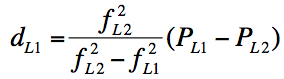
Dispersion. The ionosphere is dispersive for radio waves, which means that the GNSS ionospheric signal delay is a function of the frequency of the signal. If pseudorange measurements from more than one frequency are available, for instance from dual-frequency GPS receivers, this can be used for enhanced modeling of the ionospheric effect by using combinations of the measurements made on both frequencies.
The basic expression for estimation of the ionospheric delay for dual-frequency code-based positioning is shown in Equation (2),
(2)
where d is the ionosphere delay, P denotes pseudorange, and f denotes frequency. The subscript notation L1 and L2 refers to the GPS L1 and L2 frequencies, respectively.
For high-accuracy carrier-phase-based positioning, an ionosphere-free combination of carrier-phase observations of the L1 and L2 frequencies is often used to reduce the effect of the ionospheric phase advance in the positioning process.
Estimating the ionosphere delay with Equation (2) for code observations or utilizing the ionosphere-free combination of the phase observations compensates for the first order ionospheric effect. This is the major part of the effect, but higher order effects are present, and the size of the residual higher order effects is increased (up to some centimeters) when the ionospheric activity is increasing.
For high-accuracy applications, the difference in the time of transmission and reception of the satellite signals of the various frequencies also must be considered as the signals on various frequencies are not transmitted from the satellites (nor received at a GNSS receiver) at exactly the same time epochs. These differences are normally referred to as the satellite and receiver differential code biases.
It is important also to note in this context that the noise level on the pseudorange corrected for the ionosphere and on the ionosphere-free carrier-phase observation is increased compared to using the pure single-frequency observations for positioning, but nevertheless these first-order approaches are used successfully in most software and receiver firmware for dual-frequency positioning.
Further developments of ionosphere-free combinations will evolve in the future as the new GPS L5 frequency and the new Galileo and GLONASS frequencies become fully available for multi-frequency ionosphere-free combinations. These more advanced combinations have the potential to further reduce the residual effect of the ionospheric delay in the positioning process.
Summing up, the GNSS signal delay caused by the ionosphere is a function of the electron density of the ionosphere. But what is driving the variation in electron density, and how do we know if it is changing?
Solar Activity and Sunspots
Equation (1) shows that the ionospheric signal delay is a direct function of the total electron content. The number of free electrons in the ionosphere is not constant; it varies significantly with time and space. The number of free electrons is driven by the ionization and recombination processes of the ionosphere, and these processes are in turn driven mainly by extreme ultraviolet radiation from the sun. Radiation from other cosmic sources also has an influence but it is minor compared to the effect of the solar radiation. There are also significant short-term (minutes to hours) changes caused by wave activity from the neutral atmosphere. The ionosphere itself is embedded in the neutral atmosphere — at these altitudes this is known as the thermosphere. The thermosphere is in constant movement due to waves and tides that are generated in situ or ascending from the underlying atmosphere. This thermosphere activity affects the ionosphere and causes some of the short-term variability in the electron density. However, the term “ionospheric activity” generally refers to the variability in electron density as driven by solar activity.
The fact that ionospheric activity is mainly driven by solar activity implies that the temporal variation of the electron content of the ionosphere follows a daily cycle, with the largest TEC values in the early afternoon local time, when the effect of the solar radiation has reached a maximum. Consequently, we see the lowest activity late at night just before sunrise.
There is also a geographic variability in the electron content with the highest electron density in the equatorial region and the lowest density in the high latitude regions. The latter, however, is affected by a larger variability, correlated with auroral activity.
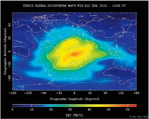
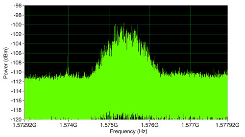
The geographic variation of TEC is illustrated with a global ionosphere map from the Center for Orbit Determination in Europe (CODE) shown in Figure 1. Global ionosphere maps are generated at CODE on a daily basis, and the maps are available on the CODE website (see Further Reading).
Figure 1. Global ionosphere map for November 22, 2010, at 14:00 UTC. (Map generated by CODE, University of Bern.)
The TEC is provided in TEC units (TECU), where one TECU equals 1016 electrons per meter squared.
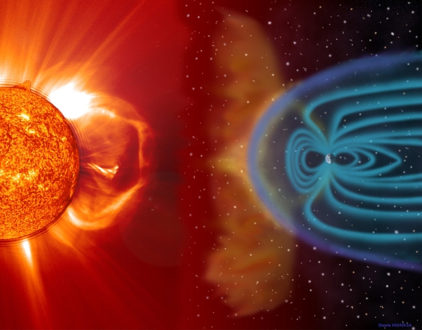
The sun also emits a constant flow of charged particles called the solar wind. The particles, mostly electrons and protons with energies between about 10 and 100 kilo-electron-volts, travel at an average speed of about 450 kilometers per second, but varying from 200 to 900 kilometers per second depending on solar activity. Although the Earth’s magnetosphere deflects most of the solar wind, the interplanetary magnetic field, which is associated with the solar wind, can cause disturbances in the geomagnetic field. When this happens, particles of the solar wind enter the geomagnetic field and cause increased ionization in the ionosphere. The solar wind therefore also has a large influence on the variability of ionospheric activity. Also, sudden eruptions of the sun such as solar flares and coronal mass ejections (CMEs) cause increased ionization and thereby a larger ionospheric variability.
Figure 2 shows a CME blast and subsequent impact at the Earth.
Figure 2. Coronal mass ejection (CME) and subsequent impact at the Earth. The left part of the illustration is composed of an image from NASA’s Solar Dynamics Observatory spacecraft superimposed on an image from the Solar and Heliospheric Observatory spacecraft jointly operated by NASA and the European Space Agency. The CME cloud arrives at the Earth about two to four days later and is shown being mostly deflected around the Earth’s magnetosphere. The blue paths emanating from the Earth’s poles represent some of its magnetic field lines. (Image: NASA/Goddard Space Flight Center.)
Solar activity and the quantity of emissions from the sun are highly correlated with the number of sunspots on its surface. A sunspot looks like a dark spot because the temperature in a sunspot is lower than that in its surroundings. The generation of sunspots is not well understood, but it is related to anomalies in the solar magnetic field. What is well known, however, is the history of the number of sunspots, because these have been observed since the early 1600s.
The number of sunspots generally follows a cycle of about 11 years. During the last few years (2007–2009), we have experienced a time period with a low number of sunspots. In fact, there were many days in a row without any sunspots visible (see Figure 3). During the next three to four years, the number of sunspots is expected to increase, and this will be followed by a decrease until we reach a new period of low solar activity in 2019–2020.
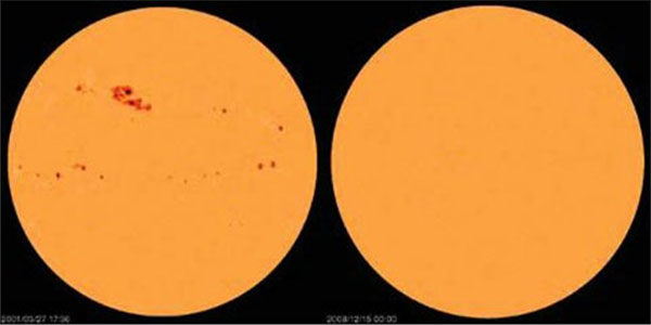
Figure 3. Images of the sun taken by the Solar and Heliospheric Observatory spacecraft. On the left is an image taken on March 27, 2001, at the peak of the last sunspot cycle. The daily sunspot count was 241. On the right is an image taken on December 15, 2008, near the minimum of the last sunspot cycle, showing no sunspots. (Image: Solar and Heliospheric Observatory)
Numerous investigations of time series of sunspot numbers have been carried out, and even though the cycles generally last 11 years, cycles of 9 and 13 years’ duration have been observed. Also, the cycles vary with respect to the maximum number of sunspots observed during a cycle, and various “cycles of cycles” appear to be present with respect to the strength of the sunspot cycles. For instance, a cycle with a period of about 420 years has been identified in the historic listings of sunspot numbers combined with other observations contributing to the knowledge of solar activity. A very low number of sunspots was observed for a number of years between 1645 and 1715 when the sun was especially calm. This period is often referred to as the Maunder Minimum after the solar astronomer Edward W. Maunder. If the theory of the 420-year cycle is correct, then we will see a period with lower solar activity and fewer sunspot numbers by the end of this century.
But let’s turn our attention to the previous and current sunspot cycles referred to as cycles number 23 and 24 (The 1755–1766 cycle is traditionally numbered “1.”). A new cycle begins with the first observed high-latitude, reversed-polarity sunspot. Reversed polarity means a sunspot with opposite magnetic polarity compared to sunspots from the previous solar cycle. Sunspots from the new and previous cycles initially coexist. Eventually, only the new-cycle sunspots are present. Cycle 24 began on January 4, 2008, when the first reversed-polarity sunspot appeared.
Analyses of observations of solar activity show that the density of the solar wind increases with increasing sunspot number. Also, with a large sunspot number, solar flares and CMEs happen more frequently. Ionospheric storm activity is more common when the sunspot number is high, and this activity increases the variability in ionospheric delays. This all adds up to an increased number of free electrons in the ionosphere and a larger variability, which provides a larger and more variable signal delay for all types of GNSS-based positioning, navigation, and timing during periods with high sunspot numbers.
We know that the sunspot number is expected to increase during the next three to four years. What can be expected and what can we do to minimize the effects of the increased ionospheric activity on positioning, navigation, and timing applications?
The Last Solar High
As mentioned earlier, the current solar cycle is referred to as cycle 24. During the last solar cycle, cycle 23, the GNSS community was alert and aware of what could happen, and therefore many events were observed and analyzed. Among the most well-known events is a sequence of storms during October and November 2003, commonly referred to as the Halloween Storms. The most extreme was the storm on October 30, 2003, which resulted from a CME on October 29 at 20:49 UTC, which subsequently impacted Earth’s magnetic field at 16:20 UTC on October 30 and produced a great geomagnetic storm, which lasted for many hours.
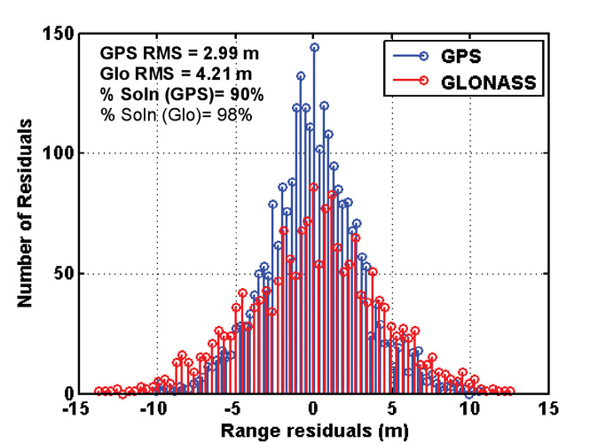
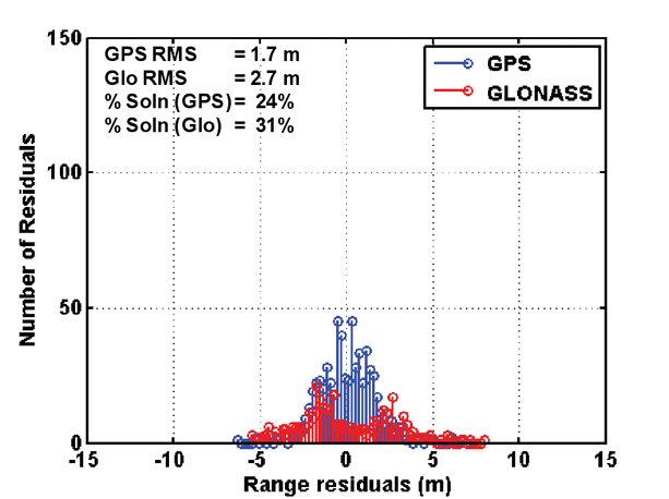
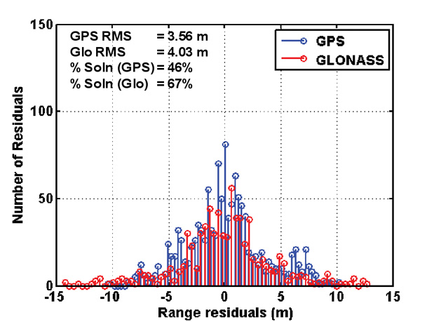
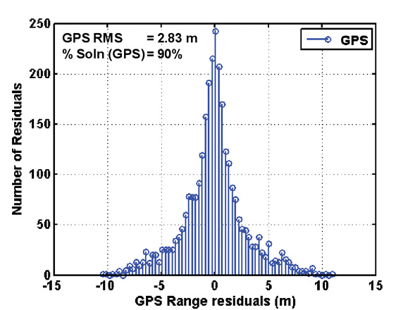
Effects on GPS positioning of this storm have been documented by the GNSS research group of the Royal Observatory of Belgium, where kinematic analyses of data from 36 GNSS stations in Europe showed position errors of more than 10 centimeters in the horizontal and up to 26 centimeters in the vertical between 21:00 and 22:00 UTC on October 30. The position errors were largest for locations in northern Europe including Sweden and Norway. The data analysis was carried out using high-quality carrier-phase data, and the processing was based on using an ionosphere-free linear combination of observations from the L1 and L2 frequencies, whereby the first-order effect of the ionosphere is removed from the results. The position errors are thus caused by mainly higher order ionospheric effects.
For navigation-grade GPS positioning, a U.S. National Atmospheric and Oceanic Administration technical memorandum (see Further Reading) reported that the Wide Area Augmentation System (WAAS) vertical error limit of 50 meters was exceeded for a period of about 11 hours on October 30, 2003. This means that, in practice, WAAS was not available for precision aircraft approaches during that time. The European Geostationary Navigation Overlay Service (EGNOS) was not transmitting during the storm, but simulations carried out later by ESA showed that the boundary regions of the EGNOS coverage area would have been especially affected by a reduction in service availability of about 20–60 percent during that day. The simulations also showed, however, that in the center of the EGNOS coverage area (in the vicinity of northern Italy), the effect would have been much smaller with a reduction in service availability of only 5–6 percent over the day.
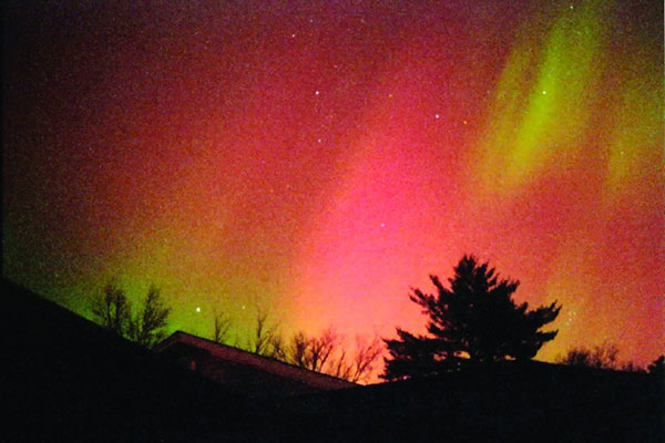
Such large storms are also often accompanied by displays of aurora (aurora borealis and aurora australis) at lower latitudes than normal. Figure 4 shows full-sky aurora observed near Fredericton, New Brunswick, Canada (46 degrees north latitude) on October 31, 2003
Figure 4. Photo of red and green auroras observed near Fredericton, New Brunswick, Canada (46 degrees north latitude) early on October 31, 2003. (Courtesy of Richard and Marg Langley.)
During a storm event on November 20, 2003, auroral activity was visible at mid-latitudes over most of North America as far south as Florida and in southern Europe including Italy and Greece.
Eruptions of the sun, often occurring in connection with high sunspot numbers, can have other effects besides the influence on GNSS-based positioning, navigation, and timing. Power-grid blackouts are known to have happened because of geomagnetic storms in connection with the sunspot peaks of both cycles 22 and 23 in 1989 and in 2003, respectively. For instance, the southern part of Sweden experienced a power blackout for several hours during the evening of October 30, 2003.
Also, orbiting satellites can experience problems with the increased radiation and solar wind density. Solar panels are, for instance,
susceptible to increased aging. And many types of satellite communication can be affected by increased ionospheric activity, not only GNSS satellite signals. Signals used for satellite phones, satellite TV, and so on can be affected.
Another phenomenon that can affect GNSS positioning is solar radio storms (also referred to as solar radio bursts) caused by events on the sun, often a solar flare, which creates radio waves that are emitted from the solar atmosphere and can propagate to the Earth where they cause an increased noise level in radio signals. Solar radio storms can cover a wide range of frequencies, including the frequencies used for GNSS. One such storm occurring on December 6, 2006, did affect GNSS positioning. With an increased noise level on the satellite signals, GNSS performance is reduced. If the noise level becomes too large, as a consequence of, for instance, a solar radio storm, GNSS receivers will lose lock on the GNSS signals, whereby positioning performance is further reduced or positioning might even be impossible. Solar radio storms are expected to happen more frequently during the peak of a solar cycle, but the event in December 2006 happened during a period with low solar activity, highlighting the fact that GNSS performance can be affected at any time, even when the sunspot number is low.
Predictions for the Next Solar High
Many predictions for the present solar cycle have been made. Because of the very long period with low solar activity during 2007–2009, some predictions expected a sudden outburst of activity and a very large cycle maximum, while other predictions foretold another increase in solar activity might not occur for many years.
However, with a general increase in the number of sunspots during 2010, it looks like we are now well into solar cycle number 24. Things can still change, but the current predictions say the maximum of the current solar cycle will be lower than the maximum of the last cycle encountered in 2001.
Predictions of sunspot numbers are based on history, logged information on sunspot numbers, and on observations of related geomagnetic activity.
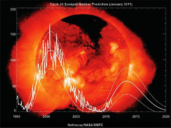
The latest prediction for the current cycle as generated by NASA is shown in Figure 5.
Figure 5. Sunspot cycle 23 and predictions for cycle 24 from NASA’s Marshall Space Flight Center. (Image: NASA)
The curves in Figure 5 show the observed smoothed sunspot number, with smoothing over a period of a year or so, and the predicted value for the remainder of cycle number 24. The dotted lines indicate the observed or expected range of the monthly-averaged sunspot numbers. The plot is updated every month as new data is obtained.
The current prediction for cycle 24 gives a smoothed sunspot number maximum of about 59 in June/July of 2013. This peak is much lower than that of the previous cycle. We are currently two years into cycle 24 and the predicted size continues to fall. According to forecasters, predicting the behavior of a sunspot cycle is fairly reliable once the cycle is well under way (about three years after the minimum in sunspot number occurs). Prior to that time, the predictions are less reliable but nonetheless equally as important.
Even though the maximum of the current solar cycle is expected to be lower than the last peak, it is important for GNSS users to be aware of the effects to be expected during the coming years.
Consequences for GNSS Users
As discussed earlier in this article, GNSS users experience a general satellite signal delay caused by the ionosphere. This signal delay is always present but varies in size. The delay is generally well modeled by most receivers and software to an extent that makes GNSS useable for all of the purposes we know today.
During enhanced ionospheric activity, GNSS users can experience residual ionospheric effects, which can cause reduced positioning, navigation, and timing performance. In such cases, dual-frequency receivers might improve the situation because of the enhanced possibilities for handling the ionospheric effect with dual-frequency data.
During enhanced ionospheric or geomagnetic storm activity caused by sudden eruptions of the sun, increased ionospheric variability will occur. Apart from causing an increased ionospheric signal delay, and thereby increased residual effects in the positioning process, this will also cause increased scintillation effects. These might cause GNSS receivers to lose lock on some or all GNSS satellite signals, reducing performance of the GNSS receiver. In the few very worst cases, GNSS-based positioning, navigation, and timing might not be possible at all for a short interval of time during very high ionospheric activity.
These worst-case scenarios are more prone to happen close to the peak of a solar cycle, which we will meet next during 2013–2014.
However, it is worth noting that for the next peak of the solar cycle, we are much better prepared for the consequences than during the last cycle. GNSS software and receiver technology has been improved to better resist the challenges of increased ionospheric activity during this solar cycle. The improvements are based on experiences gained during the last solar cycles and are to the benefit of many GNSS users. For example, users of wide area augmentation systems such as WAAS and EGNOS have correction and integrity information available, which can be a great help in identifying time epochs when positioning and navigation solutions might not be trustable because of increased ionospheric activity. The integrity information is transmitted from geostationary satellites, and during time periods with extremely high ionospheric activity, the signals with integrity information might be disrupted. This should, however, be detected by the GNSS receiver, so warning messages will be displayed for navigators.
High-accuracy real-time kinematic (RTK) positioning is today often carried out with RTK correction data from a service provider generated using a network of reference stations. Here, indications of increased ionospheric activity can be detected by the software operated by the service provider, and warnings can be distributed to the RTK users.
Warning systems have been improved, and a number of sites on the Internet provide information on current and predicted ionospheric activity (see Further Reading).
Also, in the future, GNSS users will be able to benefit from the increased number of GNSS frequencies available. These frequencies open up opportunities for new and improved methods for correction of the ionospheric delay to the benefit of users who will experience more stable and reliable GNSS performance.
Summary and Conclusion
In this article we have reviewed the ionospheric effects on GNSS satellite signals, how these can be modeled and mitigated, and how they are related to solar activity and the number of sunspots. We have also described how sudden eruptions of the sun can cause increased ionospheric activity and how these events are often correlated with a high sunspot number. Some examples of consequences for GNSS users during the last solar high have been provided, and we have evaluated the predictions for the next solar high and possible consequences for GNSS users.
We are heading towards a period of increased solar activity. GNSS users must expect more disturbances compared to what we have seen for the last four to five years. The peak of the current solar cycle is expected to be lower than the last peak, and therefore consequences for GNSS users should also be less significant. Most of the time GNSS will work very well. But we will likely see a few days with major effects, and since the number of GNSS users is increasing, the overall consequences might also be more severe, not because the ionospheric activity is worse, but simply because more people will be affected.
ANNA B.O. JENSEN is the owner of AJ Geomatics in Copenhagen and a part-time associate professor of the National Space Institute at the Technical University of Denmark (DTU Space). She has a Ph.D. from the University of Copenhagen with co-supervision from the University of Calgary, and has worked in research and development within GNSS and geodesy for more than 15 years. Her current research interests include ionospheric modeling, high accuracy positioning, and navigation in the Arctic.
CATHRYN MITCHELL is a professor in the Department of Electronic and Electrical Engineering at the University of Bath in the United Kingdom and heads the INVERT Centre, which studies inverse problems and tomography over a range of scientific fields, including navigation, space science, and medical imaging. She has a Ph.D. from the University of Wales in Aberystwyth. Mitchell has a particular interest in the use of GNSS measurements to characterize and map the ionosphere.
FURTHER READING
• Introduction to the Ionosphere and Its Effects on GNSS
“The Perfect Solar Storm” by D.N. Baker and J.L. Green in Sky & Telescope, Vol. 121, No. 2, February 2011, pp. 28–34.
Severe Space Weather Events–Understanding Societal and Economic Impacts: A Workshop Report by the National Research Council Committee on the Societal and Economic Impacts of Severe Space Weather Events, published by National Academies Press, Washington, D.C., 2008; available on line: http://www.nap.edu/openbook.php?record_id=12507.
“Combating the Perfect Storm: Improving Marine Differential GPS Accuracy with a Wide-Area Network” by S. Skone, R. Yousuf, and A. Coster in GPS World, Vol. 15, No. 10, October 2004, pp. 31–38.
“Space Weather: Monitoring the Ionosphere with GPS” by A. Coster, J. Foster, and P. Erickson in GPS World, Vol. 14, No. 5, May 2003, pp. 42–49.
The High-Latitude Ionosphere and its Effects on Radio Propagation by R.D. Hunsucker and J.K. Hargreaves, published by Cambridge University Press, Cambridge, U.K., 2002.
“GPS, the Ionosphere, and the Solar Maximum” by R.B. Langley in GPS World, Vol. 11, No. 7, July 2000, pp. 44–49.
• The Effects of the Halloween Storms on GNSS
“Impact of the Halloween 2003 Ionospheric Storm on Kinematic GPS Positioning in Europe” by N. Bergeot, C. Bruyninx, P. Defraigne, S. Pireaux, J. Legrand, E. Pottiaux, and Q. Baire in GPS Solutions, Online First, 2010, doi: 10.1007/s10291-010-0181-9.
“Assessment of EGNOS Performance Under Worst-Case Ionospheric Conditions (Solar Storm of October/November 2003)” by C. Montefusco, J. Ventura-Traveset, B. Arbesser-Rastburg, F. Froment, D. Flament, E. Tapias, S. Radicella, and R. Leitinger in EGNOS – The European Geostationary Navigation Overlay System – A Cornerstone of Galileo, ESA SP-1303, published by the European Space Agency Publications Division, Noorwijk, The Netherlands, 2006, pp. 259–268.
Halloween Space Weather Storms of 2003 by M. Weaver, W. Murtagh, C. Balch, D. Biesecker, L. Combs, M. Crown, K. Doggett, J. Kunches, H. Singer, and D. Zezula, NOAA Technical Memorandum OAR SEC-88, published by the Space Environment Center, National Oceanic and Atmospheric Administration, Office of Oceanic and Atmospheric Research, Boulder, Colorado, June 2004; available on line: http://www.swpc.noaa.gov/Services/HalloweenStorms_assessment.pdf
• Ionospheric Models and Corrections
“Ionospheric Delay Corrections for Single-Frequency GPS Receivers over Europe Using Tomographic Mapping” by D.J. Allain and C.N. Mitchell in GPS Solutions, Vol. 13, No. 2, 2009, pp. 141–151, doi: 10.1007/s10291-008-0107-y.
“Ionospheric Time-Delay Algorithm for Single-Frequency GPS Users” by J.A. Klobuchar in IEEE Transactions on Aerospace and Electronic Systems, Vol. AES-23, No. 3, May 1987, pp. 325–331, doi: 10.1109/TAES.1987.310829.
“Global Ionosphere Maps Produced by CODE” on the website of the Astronomical Institute of the University of Bern, Bern, Switzerland: http://aiuws.unibe.ch/ionosphere/.
• Solar Cycle and Solar Weather Predictions:
“Solar Weather Event Modelling and Prediction” by M. Messerotti, F. Zuccarello, S.L. Guglielmino, V. Bothmer, J. Lilensten, G. Noci, M. Storini, and H. Lundstedt in Space Science Reviews, Vol. 147, 2009, pp. 121–185, doi: 10.1007/s11214-009-9574-x.
“Predicting Solar Cycle 24 and Beyond” by M.A. Clilverd, E. Clarke, T. Ulich, H. Rishbeth, and M.J. Jarvis in Space Weather, Vol. 4, S09005, 2006, doi: 10.1029/2005SW000207.
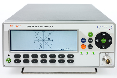
Spectracom, a global provider of time and frequency test and measurement solutions, will make available its new 16-channel GPS constellation simulator, the Pendulum GSG-55, in March. The GSG-55 is the latest in the Pendulum line of GPS receiver test instruments and part of its solution set for receiving, distributing, and validating GNSS systems.
With the enhanced signal generating capability of the GSG-55, it is possible to simulate Satellite-Based Augmentation Systems (SBAS), the company said. Navigation systems that use SBAS can improve the accuracy and reliability provided by the GPS satellite signals alone, enabling critical applications such as aircraft navigation, and surveying and mapping. SBAS simulation (support for Europe’s EGNOS and North America’s WAAS) is a new feature in the GSG-55. It is also able to generate white noise, making it possible to test receiver sensitivity under different signal-to-noise ratios.
“Many high-end GPS applications utilize 12-channel GPS receivers. Our new GSG-55 GPS constellation simulator can fully test those receivers with additional signals for more comprehensive testing in both development and production environments,” says Staffan Johansson, product manager at Spectracom.
The GSG-55 builds on the popular Pendulum GSG-54 eight-channel simulator including accurate testing of GPS timing receivers and portability through its compact and lightweight bench-top chassis. The GSG-55 also continues the Pendulum brand hallmark of ease-of-use. As such, the entire GSG family of GPS simulators has been improved based on customer feedbac, the company said.
By David W. Affens, Roy Dreibelbis, James E. Mentall, and George Theodorakos
In 1997, a Canadian government study determined that an improved search and rescue system would be one based on medium-Earth orbit satellites, which can provide full global coverage, can determine beacon location, and would need fewer ground stations. This month’s column examines the architecture of the GPS-based Distress Alerting Satellite System and takes a look at early test results.
INNOVATION INSIGHTS by Richard Langley
IT IS NOT COMMONLY KNOWN that the GPS satellites carry more than just navigation payloads. Beginning with the launch of the sixth Block I satellite in 1980, GPS satellites have carried sensors for the detection of nuclear weapons detonations to help monitor compliance with the Non-Proliferation Treaty. The payload is known as the Nuclear Detonation (NUDET) Detection System (NDS) and is jointly supported by the U.S. Air Force and the Department of Energy.
And now a third task is being assigned to the GPS satellites — that of search and rescue. Since the mid-1980s, a combination of low Earth orbit (LEO) and geostationary orbit (GEO) satellites have been used to detect and locate radio beacons activated by mariners, aviators, and others in distress virtually anywhere in the world and at any time. Some 28,000 lives have been saved worldwide since the search and rescue satellite-aided tracking, or SARSAT, system was implemented.
But the current system has some drawbacks. LEO satellites can determine a beacon’s position using the Doppler effect but their field-of-view is limited and one of them may not be in range when a beacon is activated. Furthermore, a large number of ground stations is needed to relay data from these satellites to search and rescue authorities. GEO satellites, on the other hand, have a large field of view (although missing parts of the Arctic and Antarctic), but they cannot position a beacon unless its signal contains location information provided by an integral satellite navigation receiver.
In 1997, a Canadian government study determined that a better SARSAT system would be one based on medium Earth orbit (MEO) satellites. A MEO system can provide full global coverage, determine beacon location, and do this with fewer ground stations. GPS was identified as the ideal MEO constellation.
And so was born the Distress Alerting Satellite System (DASS) that will become fully operational on Block III satellites. But already nine GPS satellites are hosting prototype hardware that is being used for proof-of-concept testing.
In this month’s column, we examine the architecture of DASS (including its relationship with the NDS), and take a look at some of the very positive test results already obtained — results that support the claim that DASS will take the search out of search and rescue.
NASA, which pioneered the technology used for the satellite-aided search and rescue capability that has saved thousands of lives worldwide since its inception nearly three decades ago, has developed new technology that will more quickly identify the locations of people in distress and reduce the risk to rescuers.
The Search and Rescue (SAR) Mission Office at the NASA Goddard Space Flight Center, in collaboration with several government agencies, has developed a next-generation satellite-aided search and rescue system, called the Distress Alerting Satellite System (DASS). NASA, the National Oceanic and Atmospheric Administration (NOAA), the U.S. Air Force, the U.S. Coast Guard, and other agencies are now completing the development and testing of the new system and expect to make it operational in the coming years after a complete constellation of DASS-equipped satellites is launched.
When completed, DASS will be able to almost instantaneously detect and locate distress signals generated by emergency beacons installed on aircraft and maritime vessels or carried by individuals, greatly enhancing the international community’s ability to rescue people in distress, This improved capability is made possible because the satellite-based instruments used to relay the emergency signals will be installed on the GPS satellites.
A recent satellite-aided rescue started on June 10, 2010, when 16-year-old Abby Sunderland on her 40-foot (12.2-meter) sailboat “Wild Eyes” encountered heavy seas approximately 2,000 miles (3,200 kilometers) west of Australia in the Indian Ocean. Her sailboat was dismasted and an emergency situation resulted. Ms. Sunderland activated her two emergency beacons whose signals were picked up by orbiting satellites. Using coordinates derived from the signals, a search plane spotted Ms. Sunderland the next day, and a day later she was rescued by a fishing boat directed to the scene. This highly publicized event is one of thousands of successful rescues made possible by years of NASA research and development.
Background
The beginnings of satellite-aided search and rescue date back to 1970, when a plane carrying two U.S congressmen crashed in a remote region of Alaska. A massive search and rescue effort was mounted, but to this day, no trace of them or their aircraft has ever been found. At the time, search for missing aircraft was conducted by search aircraft flying over thousands of square kilometers hoping to sight the missing aircraft. As a result of this tragedy, Congress recognized this inefficient search method and passed an amendment to the Occupational Safety and Health Act of 1970 requiring most aircraft flying in the United States to carry emergency locator beacons (ELTs) to provide a local homing capability. NASA then developed the technology to detect and locate an ELT from ground stations using the beacon signal relayed by satellites to provide more global coverage. This concept evolved into a highly successful international search and rescue system called COSPAS-SARSAT (COSPAS is an acronym for the Russian words “Cosmicheskaya Sistema Poiska Avariynyh Sudov,” which translates to “Space System for the Search of Vessels in Distress;” SARSAT is an acronym for Search and Rescue Satellite-Aided Tracking). Established by Canada, France, the United States, and the former Soviet Union in 1979, the system has 43 participating countries and has been instrumental in saving more than 28,000 lives worldwide, including 6,400 in the U.S. — all as a result of NASA’s innovations.
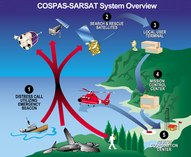
Since this auspicious beginning, NASA has continued to perform SAR research and development as a member of the National Search and Rescue Committee, and supports the National Search and Rescue Plan through an interagency memorandum of understanding with the Coast Guard, the Air Force, and NOAA. NOAA is responsible for operation of the U.S. portion of current COSPAS-SARSAT system that relies on SAR payloads on weather satellites in low-earth and geostationary orbits. As shown in Figure 1, the satellites relay distress signals from emergency beacons to a network of ground stations and ultimately to the U.S. Mission Control Center (USMCC) operated by NOAA. The USMCC distributes the alerts to the appropriate search and rescue authorities: the U.S. Air Force or the Coast Guard. The Air Force coordinates search and rescue for the mainland U.S. SAR region and operates the Air Force Rescue Coordination Center. The Coast Guard performs maritime search and rescue and oversees the U.S. national SAR policy.
FIGURE 1. Overall concept of search and rescue system. (Image: Cospas-Sarsat)
Beacons
Three types of distress emergency locator beacons are in use that are compatible with the COSPAS-SARSAT system:
EPIRBs (emergency position-indicating radio beacons) designed for maritime use.
ELTs (emergency locator transmitters) for use on aircraft.
PLBs (personal locator beacons) for personal use. These can be used by persons engaged in high-risk activities such as mountain climbing and backcountry skiing.
Originally, emergency locator beacons transmitted an analog signal on two frequencies: 121.5 MHz and 243 MHz in the civil and military aeronautical communications bands, respectively, so that they would be audible over aircraft radios. Later, a signal that was encoded with a digital message and transmitted at 406 MHz was added. Since February 1, 2009, only the 406-MHz-encoded signals are relayed by satellites supporting the international COSPAS-SARSAT system. Therefore, older beacons that only transmit the 121.5/243-MHz signals are now only detectable by ground-based receivers and aircraft overflying a crash site.
The 406-MHz beacons transmit an approximately half-second message, or burst, approximately every 50 seconds, beginning 50 seconds after being activated. The actual time of burst transmission is dithered in time so that no two beacons will have all of their bursts coincident. A 406-MHz beacon may also have an integral global navigation satellite system (GNSS) receiver. Such a beacon uses the GNSS receiver to attempt to determine its location for inclusion in the transmitted digital message. In this way, the beacon will be located once it is detected by a low-Earth-orbit (LEO) or geostationary orbit (GEO) satellite.
Distress messages contain information such as:
The beacon’s country of origin.
A unique 15-digit hexadecimal beacon ID.
Location, when equipped with an integrated GNSS receiver.
Whether or not the beacon contains a 121.5-MHz homing signal.
Room for Improvement
SARSAT first became operational in the mid-1980s. The current system uses instruments placed on LEO and GEO weather satellites to detect and locate mariners, aviators, and recreational enthusiasts in distress almost anywhere in the world at anytime and in almost any condition. Previously, dedicated Russian LEO satellites were also implemented but the use of these satellites was discontinued in 2007.
Although it has proven its effectiveness, as evidenced by the number of persons rescued over the system’s lifetime, the current capability does have limitations. LEO spacecraft orbit the Earth 14 times a day and use the Doppler effect with satellite orbital ephemeris data to calculate the position of a beacon. However, a satellite may not be in a position to pick up a distress signal the moment a user activates the beacon. Time is critical in responding to an emergency situation. Unfortunately, delays of two hours or longer are possible, especially near the equator.
LEO spacecraft carry two instruments: a Search and Rescue Repeater (SARR) supplied by the Canadian Department of National Defence, and a Search and Rescue Processor (SARP) provided by the French Centre National d’Etudes Spatiales (CNES). The SARR is a pure repeater, which relays the beacon signal to a local ground station where the data is analyzed to obtain a location. The SARP processes the received beacon signal by measuring the Doppler shift as a function of time, and decoding the digital message included in the 406-MHz signal. This information is stored until it can be transmitted to a ground station using the SARR’s downlink transmitter. Under most conditions beacon locations can be determined to within a radius of 5 kilometers.
Geostationary weather satellites, on the other hand, orbit above the Earth in a fixed location over the equator. Although they do provide continuous visibility of much of the Earth, they cannot independently locate a beacon unless it contains a GNSS receiver that determines its position and includes it in the beacon’s digital message. Currently, not all beacons contain integral GNSS receivers. Furthermore, even if a beacon contains a GNSS receiver, the navigation signal may be obstructed by terrain or thick foliage.
The next-generation system, DASS, overcomes these limitations and will improve accuracy and response time to provide an even more capable life-saving system.
Distress Alerting Satellite System
A 1997 Canadian government study of possible alternative satellite systems for SARSAT, including commercial sources, determined that the ideal system is based on medium Earth orbit (MEO) satellites. A MEO system will be able to provide superior global detection and location data with fewer ground stations than the existing COSPAS-SARSAT system. The GPS constellation was identified as an ideal MEO platform.
The concept of the DASS system is straightforward. Three or more antennas track different GPS satellites equipped with search and rescue repeaters that receive the distress signal and retransmit the signal to the ground. Since each satellite is in a different orbit, each received signal has a different Doppler-shifted arrival frequency and time of arrival. Knowing the position and orbit of each satellite, it is possible to determine the position of the distress beacon.
Future improvement in location accuracy is made possible by one of the strengths of the DASS space segment. That is, the DASS location algorithm optimizes location accuracy utilizing time and frequency measurements of beacon signals that were not designed for that purpose. The DASS space segment allows for the beacon signal to be modified in the future, enhancing the performance of this type of location process.
Other advantages of DASS over the existing system are fairly obvious. Reception of the emergency signal is immediate. Locations can be determined after receiving a single beacon burst since it does not rely on measuring the Doppler shift over time to determine position, as in the current LEO system. A full constellation of DASS-equipped GPS satellites in orbit will ensure that four or more satellites are in view of the transmitting emergency beacon anywhere in the world while requiring fewer ground stations.
Another key strength of the DASS system is the promise of SARSAT transponders on each satellite in the large and well-managed GPS constellation. There are at least 24 GPS active satellites in orbit at any given time (currently, 31 are active). When the GPS constellation is fully populated by satellites with DASS transponders, it will provide global coverage for satellite-supported search and rescue and provide capabilities for rapid detection and location of distress beacons.
Efforts are ongoing to integrate a satellite beacon repeater instrument, to be provided by the Canadian government, onto the GPS Block III B and C satellites to provide the DASS space segment for operational use.
DASS Development
DASS development will proceed in phases referred to as the definition and development, proof of concept, demonstration and evaluation, initial operating capability, and final operating capability. The proof of concept (POC) phase was completed in January 2009. The POC testing and results are summarized in this article. At the time of this writing, preparations are ongoing to initiate the demonstration and evaluation phase.
Definition and Development. In 2000, as part of the definition and development phase, the NASA GSFC SAR Mission Office began discussions with the Department of Energy’s Sandia National Laboratories (SNL) to determine if it would be feasible to add a SAR repeater function to a Department of Energy (DOE) instrument on GPS satellites. Sandia representatives thought it possible, and NASA agreed to fund a study to determine if, with minor modification, one could include a search and rescue repeater function to their instrument. The SNL feasibility study concluded that the GPS DOE package could, with minor modifications, perform the SAR mission. The study also determined that accurate locations could be calculated after a single beacon transmission and improved with each subsequent beacon transmission. Based on this information, NASA, with the cooperation of the U.S. Air Force Space Command and SNL, proceeded with the development of the new space-based search and rescue system, which was named the Distress Alerting Satellite System.
Proof of Concept. In 2003, a memorandum of agreement (MOA) between NASA, NOAA, the Air Force, the Coast Guard, and the Department of Energy tasked NASA to perform a POC program for DASS. The MOA included the development of a POC space segment and a prototype ground station to perform post-launch checkout, performance testing, and implementation planning of an operational DASS system. It stressed the need for DASS, gave authority to each participating agency to participate in the POC demonstration, and defined the roles of each.
The Air Force Space Command approved the addition of modified equipment on GPS satellites. The DASS POC space segment operates as a subcomponent of GPS Block IIR and IIF satellites. Nine GPS Block IIR satellites carry experimental DASS payloads, and all 12 IIF satellites are scheduled to. Therefore, the final POC space segment will consist of 21 DASS-equipped GPS satellites. Each payload receives 406-MHz SAR signals on an extant GPS UHF antenna and relays the signals at a GPS S-band frequency on a second extant antenna.
It is important to note that the performance of the DASS POC space segment will be exceeded by the performance of the operational space segment being designed specifically for DASS and planned for launch on GPS Block III satellites.
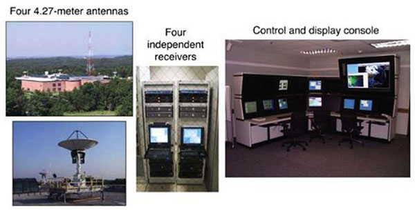
A prototype DASS ground station (Figure 2) was funded by NASA and installed at GSFC. The DASS prototype ground system consists of four antennas, four receivers, and the workstations and servers necessary to process the received data, command and control the operation of the ground station, and display and analyze the results. The antennas are located on the corners of the roof of a building connected by fiber-optic cable to signal processing equipment located in another building two kilometers away.
FIGURE 2. Prototype ground station at NASA GSFC. (Images: NASA)
Proof of Concept Testing
The overall objectives of the POC tests were to demonstrate the effectiveness of the DASS concept and to define its technical and operational characteristics. The primary technical objective was to demonstrate the system’s ability to detect and locate 406-MHz emergency beacons under various controlled conditions. This is the most important measure of the system’s ability to perform as expected.
The specific objectives of the DASS POC demonstration were to
Confirm the expected performance of the DASS concept.
Determine if new or enhanced requirements needed to be established.
Define preliminary performance levels that will be used to establish the scope and content of the next phase of development, referred to as the demonstration and evaluation phase.
Therefore, during POC testing, performance measurements were taken for the probability of detection, probability of location, and location accuracy, defined as follows.
Probability of detection is the probability of detecting the transmission of a 406-MHz beacon and recovering a valid beacon message from any available satellite.
Probability of location is the probability of obtaining a location solution within a given time after beacon activation, independently of any encoded position data in the 406-MHz beacon message.
Location accuracy is the distance from the location solution obtained within 5 minutes after beacon activation, to the actual beacon location. The required performance is specified as the probability that a given solution is within a given distance of the actual location.
It is important to note that the predicted performance of DASS assumes a full constellation of DASS-equipped GPS satellites. In fact, one of the key strengths of DASS is the promise of DASS transponders on each satellite in the GPS constellation. When a full constellation is equipped with DASS transponders, there will typically be between seven and 13 GPS satellites visible at the NASA ground station. Thus, it will be possible to schedule the ground-station antennas to receive data from the best satellites in terms of geometry, signal strength, processing capability, and other factors.
However, at the time of the POC testing, there were only eight GPS satellites equipped with DASS transponders. A maximum of three DASS-equipped GPS satellites were visible at the same time at the NASA ground station (above a 15-degree elevation angle), and there were times when only one DASS-equipped GPS satellite was visible. Thus, it was impossible to optimize satellite selection since there was never an opportunity to select from an excess of satellites that a full constellation would provide.
In particular, satellite geometry and its effect on performance is never as optimal as what would be obtained from a full constellation of GPS satellites. To predict the results of a full constellation using the results from a severely reduced constellation, a calculation based on “dilution of precision” was used.
Dilution of precision (DOP) or geometric dilution of precision, to be specific, is used to describe the geometric strength of satellite configuration on GPS accuracy. When visible satellites are close together in the sky, the geometry is said to be weak and the DOP value is high; when far apart, the geometry is strong and the DOP value is low. Thus a low DOP value gives rise to a better GPS positional accuracy due to the wider angular separation between the satellites used to calculate a beacon’s position.
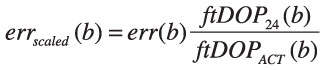
Location accuracy results can be scaled to reflect the true DOP that would be obtained by a satellite constellation of 24 GPS satellites. The DOP error caused by uncertainty in time and frequency measurements is used for scaling. The DOP of the satellites actually used to calculate a location solution, denoted by ftDOPACT, is always bigger than the DOP that would have been available from a constellation of 24 GPS satellites, ftDOP24. The raw location errors need to be multiplied by the ratio ftDOP24 / ftDOPACT to reflect the results that would have been obtained if all 24 satellites were present.
The raw average location error, erravg, is given by the following:
err(b) = err(lat(b),lon(b))= distance from the known location to (lat(b),lon(b))
erravg(b0) = err(latavg(b0),lonavg(b0))
where Ω(b0) is the set of seven or fewer consecutive burst locations within 5 minutes, starting with burst b0.
The scaled location error is the location error scaled by the DOP ratio:
Since DOP changes little over 5 minutes, the error of the average is approximately
where ftDOPACT(b) is the time-frequency DOP of burst b calculated with either three or four satellite geometries depending on
the number of measurements used in the location calculation.
Test Source
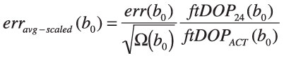
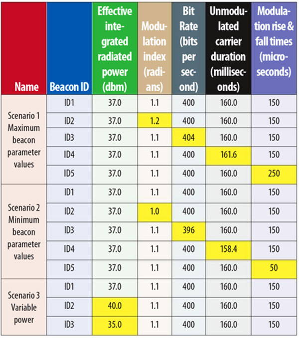
A custom-designed beacon simulator was used to generate the transmissions of multiple COSPAS-SARSAT 406-MHz beacons over an extended period of time. To represent expected operational realism in the tests, the beacon simulator was used to transmit beacons at the limits of the five major beacon parameters specified by COSPAS-SARSAT as well as the nominal values. The five major beacon parameters are transmit power, modulation index, bit rate, un-modulated carrier duration, and modulation rise and fall times (see TABLE 1).
During POC testing, five beacons were transmitted using three scenarios: maximum beacon parameter values, minimum beacon parameter values, and variable power. The parameter values changed in each test scenario and are highlighted in TABLE 2. Beacon detection and location performance is measured for periods when there are three or more satellites visible at the same time, and for durations sufficient to collect a statistically significant amount of data.
Table 2. Beacon parameter values for each test scenario. (Data: Authors)
Two characteristics of the test source that affect system performance are the beacon antenna pattern and ground mask. To simulate beacons, the beacon simulator has a monopole antenna with the gain pattern shown in Figure 3. There is a substantial reduction in the transmitted signal at high-elevation angles (above 60°). DASS-equipped GPS satellites are often at high-elevation angles during a typical day. As expected, the effect of the pattern on test results can clearly be seen upon close inspection of the data. However, the beacon antenna pattern is an unavoidable reality and is, therefore, fully represented in the data used to generate the results presented here. Additionally, there were significant ground obstructions of the beacon signal in certain directions. The effect of beacon antenna pattern is fully included in the results presented in this article, but ground mask is taken into account by limiting satellite visibility to an elevation cut-off angle of 15 degrees.
FIGURE 3. Beacon simulator transmit antenna gain pattern.
POC Test Results
In this section, we discuss the POC test results in terms of probability of detection, probability of location, and location accuracy.
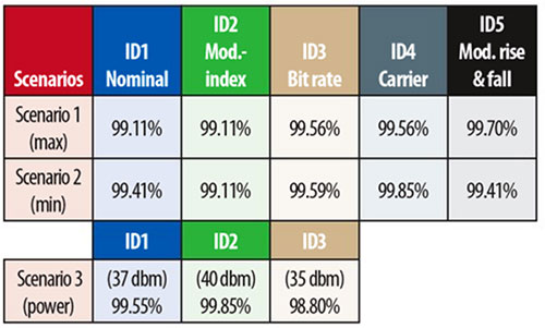
Probability of Detection. As previously mentioned, probability of detection is the probability of detecting the transmission of a 406-MHz beacon and recovering a valid beacon message from any available satellite. The requirement is that 95 percent of individual transmitted messages are detected.
Test results are given in TABLE 3 and show that the probability of detection is approximately 99 percent for all scenarios, even though only three satellites were in view at a time. Obviously, the probability of detection is dependent on the number of available satellites and performance would improve with continuous coverage by four or more satellites.
Table 3. Probability of detection test results. (Data: Authors)
Probability of Location. Again, the probability of location is the probability of obtaining a location solution within a given time after beacon activation, independently of any encoded position data in the 406-MHz beacon message. The requirement is that the probability of calculating a beacon location is 98 percent within 5 minutes.
Since the probability of location is dependent on the number of visible satellites, our performance was limited by the reduced constellation of DASS-equipped satellites. Results from periods of three-satellite coverage were 85 percent within 5 minutes, 92 percent within 10 minutes, and 94 percent within 15 minutes.
Again, the probability of location is dependent on the number of visible satellites, and performance would improve with continuous coverage by four or more satellites. To investigate the possible improvement with enhanced satellite coverage, we reduced the minimum satellite elevation angle from 15 to 10 degrees. This allowed a fourth satellite to become visible for a limited time at very low elevation angles. Even though the signal quality from such a satellite was poor, the probability of location during this period of four-satellite coverage improved as follows: 91 percent within 5 minutes, 96 percent within 10 minutes, and 97 percent within 15 minutes.
As can be seen from these results, even adding a satellite with a very low elevation-angle pass significantly improves performance. The expectation is that having a full constellation of satellites available would improve performance even more. Furthermore, the increase in satellite performance expected in the operational system will also improve probabilities of detection and location.
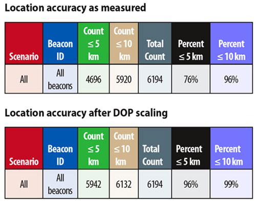
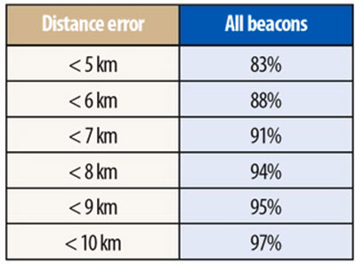
Location Accuracy. Recall that location accuracy is measured as the percentage of location solutions obtained within five minutes after beacon activation that are within five kilometers of the actual beacon location.
The requirement is to obtain 95 percent of the locations to within 5 kilometers of the actual location and 98 percent within 10 kilometers within five minutes after beacon activation.
As mentioned earlier, the requirements included in the performance specification assume a constellation of 24 DASS-equipped GPS satellites. POC testing was done with a system that had only eight DASS-equipped GPS satellites available. However, location errors can be scaled to reflect what the DOP would be if the satellite constellation contained all 24 GPS satellites. Therefore, it is the scaled results that can be used to determine whether performance will meet the requirement.
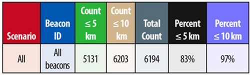
TABLE 4, therefore, presents the location accuracy results as measured, and after being scaled by DOP.
Table 4. Location accuracy for 5-minute periods. (Data: Authors)
Another important performance metric for DASS is location accuracy obtained after a single beacon burst is received. Even though there is not currently a requirement for single burst location accuracy, it is a very desirable feature of DASS since an emergency situation does not guarantee that more than a single burst will be received. Single burst location accuracy was, therefore, measured with the results shown in TABLE 5. Once again, the results are scaled by DOP values to remove the effect of non-optimal satellite geometry.
Table 5. Single burst location accuracy. (Data: Authors)
More insight into this performance can be gained by examining the single burst location accuracy distribution as a function of distance error, as shown in TABLE 6. It can be seen that, for these beacons, computed locations are within 9 kilometers of the actual location 95 percent of the time. Again, the expectation is that having a full constellation of satellites available would improve this performance. For instance, having more satellites to choose from might allow the system to select data from satellites with stronger or less noisy links.
Table 6. Single burst location accuracy by distance error. (Data authors)
Conclusion
The promise of search and rescue instruments on each satellite in the large and well-managed GPS constellation will provide a significant advancement in the capabilities of the already highly successful COSPAS-SARSAT system. The new system will provide global coverage for satellite-supported search and rescue and provide capabilities for rapid detection and location of distress beacons while requiring fewer ground stations.
The DASS POC system has validated, by test, the predictions made by analysis during the definition and development phase. The DASS POC testing has demonstrated reliable detection and accurate location of beacons within five minutes of activation. Accurate locations are also produced after even a single burst of a newly activated beacon, which is a desirable feature of DASS, since an emergency situation does not guarantee that more than a single burst will be received.
The performance obtained using a reduced constellation of satellites equipped with a modified, existing instrument not only demonstrates the existing capability, but also confirms the improvements to come with the operational system. In fact, the success of DASS is being emulated by the European Union in the design of their future Galileo GNSS constellation and the Russians in an upgraded GLONASS GNSS constellation, all of which will be interoperable by international agreement.
DASS will contribute to NASA’s goal of taking the search out of search and rescue. Achieving this goal will not only improve the chances of rescuing people in distress quickly, which is critical to their survival; it will also reduce the risk to rescuers who often put themselves in dangerous situations to affect a rescue. That is why the motto of the Search and Rescue Office is “Saving more lives, reducing risks to search personnel, and saving resources.”
David W. Affens is the manager of the NASA Search and Rescue (SAR) Mission Office at the Goddard Space Flight Center (GSFC) in Greenbelt, Maryland, where he began working in 1990. He holds a degree in electronic engineering. Before joining NASA, he worked in various aspects of submarine warfare and intelligence gathering for the U.S. Navy over a span of 21 years.
Roy Dreibelbis is a consultant who has worked in rescue-related jobs since 1957, including helicopter rescue missions in Vietnam. As an officer in the U.S. Air Force, he was the director of Inland SAR at rescue headquarters for the coterminous 48 states, was commander of the 33rd Air Rescue Squadron, and served as deputy chief of staff for rescue operations at rescue headquarters from 1979 until 1981. Upon retirement from the Air Force, he was employed by the State of Louisiana as flight operations director and chief pilot. In 1987, he accepted employment with contractors in the District of Columbia area that supported NASA and NOAA SARSAT activities.
James E. Mentall is the NASA/GSFC Search and Rescue Instrument Manager. He has a Ph.D. in physics and has spent more than 42 years of his professional life at GSFC. For 15 of those years, he has been responsible for the integration and test of the Search and Rescue Repeater and the Search and Rescue Processor on the NOAA Polar-orbiting Operational Weather Satellites. He has also served as the deputy mission manager for the Search and Rescue Mission Office and played a significant role in the procurement of the DASS antenna system and ground station.
George Theodorakos is the chief staff engineer for MEI Technologies, Inc. He received his B.S. summa cum laude and M.S. degrees in electrical engineering from the University of Maryland, College Park, Maryland, in 1978 and 1987, respectively. Since 2002, in his role as chief staff engineer at MEI, he has provided technical management support to the Search and Rescue Mission Office at GSFC.
FURTHER READING
• Distress Alerting Satellite System (DASS)
“Distress Alerting Satellite System (DASS)” on the NASA Search and Rescue Mission Office website, Goddard Space Flight Center, Greenbelt, Maryland.
• Search and Rescue Satellite-Aided Tracking (SARSAT)
“Search and Rescue,” Chapter 6 in Review of the Space Communications Program of NASA’s Space Operations Mission Directorate by the Committee to Review NASA’s Space Communications Program, Aeronautics and Space Engineering Board, Division on Engineering and Physical Sciences, National Research Council, published by the National Academies Press, Washington, D.C., 2007.
“Overview of MEOSAR System Status” by J. King, a presentation at BMW-2009, Beacon Manufacturers Workshop, St. Pete Beach, May 8, 2009.
“MEOSAR to the Rescue” by J. King in Channels, the EMS SATCOM Quarterly, published by EMS Technologies, Inc., January 31, 2007.
• Nuclear Detonation (NUDET) Detection System
“Detecting Nuclear Detonations with GPS” by P.R. Higbie and N.K. Blocker in GPS World, Vol. 5, No. 2, February 1994, pp. 48–50.
By Cillian O’Driscoll, Gérard Lachapelle, and Mohamed Tamazin, University of Calgary
The impact of adding GLONASS to HS-GPS is assessed using a software receiver operating in an actual urban canyon environment. Results are compared with standard and high sensitivity GNSS receivers and show a significant improvement in the availability of position solutions when GLONASS is added. An assisted high sensitivity receiver architecture is introduced which enables high fidelity signal measurements even in degraded environments.
High-sensitivity (HS) GNSS receivers have flourished in the last decade. A variety of advances in signal-processing techniques and technologies have led to a thousandfold decrease in the minimum useable signal power, permitting use of GNSS, in particular GPS, in many environments where it was previously impossible.
Despite these recent advances, the issue of availability remains: in many scenarios there are simply too few satellites in view with detectable signals and a good geometry to compute a position solution. Of course, one way to improve this situation is to increase the number of satellites in view. GLONASS has been undergoing an accelerated revitalization program of late, such that there are currently more than 20 active GLONASS satellites on orbit. The combined use of GPS and GLONASS in a high-sensitivity receiver is a logical one, providing a near two-thirds increase in the number of satellites available for use.
The urban canyon environment is one in which the issue of signal availability is particularly important. The presence of large buildings leads to frequent shadowing of signals, which can only be overcome by increasing the number of satellites in the sky. Even if sufficient satellites are visible, the geometric dilution of precision can often be large, leading to large errors in position.
This work focuses on the advantages of using a combined GPS/GLONASS receiver in comparison to a GPS-only receiver in urban canyons. The target application is location-based services, so only single frequency (L1) operation is considered. We collected and assessed vehicular kinematic data in a typical North American urban canyon, using a commercially available high-sensitivity GPS-only receiver, a commercial survey-grade GPS/GLONASS receiver, and a state-of-the-art software receiver capable of processing both GPS and GLONASS in standard or high-sensitivity modes.
Processing Strategies
The standard (scalar-tracking) GNSS receiver architecture is shown in Figure 1. In the context of this article, the key characteristic of a standard receiver is that the signals from the different satellites are each tracked in parallel and independent tracking channels, and usually only three correlators are used. The information from the channels is only combined in the navigation filter to estimate position, velocity, and time. In this way, there is no sharing of information between channels in order to attempt to improve tracking performance.
Figure 1. Standard receiver architecture (courtesy Petovello et al).
Within each channel, the down-converted and filtered samples from the front end (not shown in Figure 1) are then passed to a signal-processing function where Doppler-removal (baseband mixing) and correlation (de-spreading) is performed. The correlator outputs are then passed to an error-determination function consisting of discriminators (typically one for code, frequency, and phase) and loop filters. The loop filters aim to remove noise from the discriminator outputs without affecting the desired signal. Finally, the local signal generators — whose output is used during Doppler removal and correlation — are updated using the loop-filter output.
Assisted HS GNSS Receiver. The assisted HS GNSS receiver architecture used in this work is shown in Figure 2. Notable differences to the standard receiver architecture are highlighted in red.
Assistance information is provided in the form of broadcast ephemerides, raw data bits, and a nominal trajectory (position and velocity) that would normally be generated by the receiver. At each measurement epoch, the receiver uses the nominal position and velocity in conjunction with the ephemerides to compute the nominal pseudorange and pseudorange rate for each satellite in view. These parameters are passed to the signal-processing channels. Each channel evaluates a grid of correlators around the nominal pseudorange (code) and pseudorange rate (Doppler) values. The data bits are wiped off using the assistance information to permit long coherent integration times. For each signal tracked, the correlator grid is used to estimate code and Doppler offsets relative to the nominal values. These estimates are then used to generate accurate pseudorange and Doppler estimates.
The number of correlators used and the spacing of these correlators in the code and frequency domains are completely configurable. A sample correlation grid computed during live data processing is illustrated in Figure 3. Measurements are generated by choosing the three correlators nearest the peak in the search space and using a quadratic fit to determine a better estimate of the peak location. In this work, a total of 55 correlators per channel were used.
Figure 3. Sample grid of correlator points computed for GPS PRN 04.
The assisted HS receiver is initialized in static mode in an open-sky setting during which reliable clock bias and drift estimates are derived. A high-quality oven-controlled crystal oscillator was used during this initial test to ensure that the clock drift did not change significantly over the period of the test (approximately 20 minutes). The clock bias during the test is updated using the clock drift estimate.
Note that this architecture is a generalization of the vector-based architecture, where the navigation solution used to aid the signal processing can be provided by an external reference.
Navigation Solution Processing. All navigation solution results presented here are obtained in single-point mode using an epoch-by-epoch least-squares solution with the PLAN Group C3NavG2 software, which uses both code and Doppler measurements. This processing strategy enables a fair comparison amongst the different signal processing strategies, as the smoothing effect of specific navigation filters is eliminated by this approach. More realistic accuracy estimates of the measured pseudoranges can be obtained. It is understood that in an operational environment, a well-tuned filter will obtain significantly better navigation performance than the epoch-by-epoch solutions presented here.
The measurements are weighted using a standard-elevation-dependent scheme. Thus there is no attempt to tune the weighting scheme for each receiver.
Data Collection
To test the relative performance of the various processing strategies, we conducted a test in downtown Calgary. Data was collected using a commercial HS GPS receiver, a commercial survey grade GPS/GLONASS receiver, and an RF downconverter and digitizer. The digitized data was post-processed in two modes (standard and assisted HS GNSS) using the PLAN group software receiver GSNRx.
Raw measurements were logged from each of the commercial receivers at a 1-second interval. The parameters used in GSNRx are given in Table 1.
The trajectory followed is shown in Figure 4. The majority of the route was travelled in an East-West direction, with significant signal masking to the North and South. The Opening Photo shows an aerial view of downtown Calgary where the test took place. Masking angles exceeded 75 degrees along the vehicle trajectory.
Figure 4. Test Trajectory where the route is approximately 4 km with a 10 minute travel time.
A sky plot of the satellites visible above a 5-degree elevation mask at the test location is shown in Figure 5. A total of 11 GPS and seven GLONASS satellites were present.
Figure 5. Skyplot of GPS and GLONASS satellites over Calgary at the start of the test.
A static period of approximately three minutes duration was used to initialize the assisted HS GNSS processing. During this period, the vehicle had a largely clear view of the sky. Nevertheless, three satellites were blocked from view during this period, namely GPS SVs 13 and 3, and GLONASS SV 22. As a result, these SVs were not available for processing in the assisted HS GNSS mode. The two commercial receivers were already up and running prior to the initialization period and so were able to process these three low-elevation satellites when they came into view during the test. See PHOTO on next page for a typical scene during the downtown test.
Analysis
To study the impact of adding GLONASS, the analysis focuses on solution availability, the number of satellites used in each solution, the DOP associated with each solution, and the statistics of the least-squares solution residuals. In the absence of a reference solution, the statistics of the residuals nevertheless give a reasonable indication of the quality of the measurements used, provided sufficient measurements are available to ensure redundancy in the solution. Nevertheless, some pseudorange errors will be absorbed by the navigation solution, hence the statistics of the residuals can be viewed as only a good estimate of the quality of the measurements themselves.
Solution Availability. As previously discussed, the navigation processing strategy adopted is the same for all receivers used in the test. A single-point epoch-by-epoch least-squares solution is computed at a 1 Hz rate. If there are insufficient satellites in view at a given epoch, or the solution fails to converge in 10 iterations, no solution is computed. In this section, the analysis focuses on the percentage of epochs during the downtown portion of the test for which a solution was computed.
Figure 6 shows the percentage of solutions computed for each receiver processing strategy as a function of HDOP and VDOP thresholds, respectively. Thus, for example, the assisted HS GPS-GLONASS processing strategy yielded navigation solutions with a HDOP less than 6 between 80 percent and 85 percent of the time. For larger DOP thresholds, it is clear that there is little difference between GPS-only processing and GPS+GLONASS processing. The biggest differences are caused by the processing strategies employed. The advantages of HS processing are clear, at least in terms of solution availability. For this test and the particular geometry of the satellites in view during the test, GPS+GLONASS processing does yield a noticeable improvement in the VDOP, particularly at lower thresholds.
Figure 6A. Percentage solution availability versus HDOP threshold.Figure 6B. Percentage solution availability versus VDOP threshold.
Note that the standalone HS GPS receiver exhibits greater solution availability than the assisted software HS GPS-GLONASS receiver at higher DOP thresholds. This is most likely due to the low-elevation satellites that were excluded from the assisted HS processing due to their being masked during the initialization period as discussed earlier. Overall, however, there is little difference between GPS-only processing and GPS-GLONASS processing in terms of solution availability. This fact, of course, does not yield any information on the quality of the solutions obtained, which is discussed later.
To gain further insight into the impact of GLONASS, Figure 7 shows the percentage of solutions computed that exhibit redundancy. Thus, of all solutions computed during the downtown portion of the test, Figure 7 illustrates the percentage of those solutions that have redundant measurements. For GPS-only processing, this implies that five or more measurements were used in computing the position, while for GPS-GLONASS processing a minimum of six measurements were required. In this case, the advantage of using GLONASS becomes more apparent. For all processing strategies the addition of GLONASS yields an increase of 5 to 10 percent in the number of solutions with redundancy. Although not studied herein, this would have a positive impact on fault detection.
Residuals Analysis
To investigate the quality of the measurements generated by each processing strategy, the residuals from the least-squares solutions are studied. Only those epochs for which redundant solutions are computed are considered here, since non-redundant solutions lead to residuals with values of zero. As discussed above, the analysis of these residuals gives an estimate of the quality of the measurements generated.
Figure 8 shows the histograms of the residuals from all GPS-GLONASS processing strategies. Once again, it is important to emphasize that only residuals from solutions with redundancy are considered. In addition, the results presented are limited to those epochs during which the vehicle was in the downtown portion of the test. For the purposes of this presentation an upper GDOP threshold of 10 was set.
It is interesting to note that in all cases (assisted HS, standard wide correlator, and commercial survey-grade processing), the relative RMS values of the GPS and GLONASS residuals are about the same. These results indicate that, irrespective of the signal-processing strategy employed, the GLONASS measurements are of a similar quality to the GPS measurements. The number of residuals available is however different between the standard and HS solutions, as the latter produce more measurements and more redundant solutions, hence more residuals. The processing strategy obviously had a significant impact on the availability of redundant solutions as discussed in the previous section.
Figure 8A. GPS-GLONASS range residuals comparison: assisted HS-GPS-GLONASS. RMS values and the percentage of solutions used in the histogram are also shown.Figure 8B. GPS-GLONASS range residuals comparison: standard wide correlator. RMS values and the percentage of solutions used in the histogram are also shown.Figure 8C. GPS-GLONASS range residuals comparison: survey-grade receiver. RMS values and the percentage of solutions used in the histogram are also shown.
Figure 9 shows the histograms of the range residuals from GPS-only processing. In this case, the navigation solution is a GPS-only navigation solution, though in the case of the assisted HS receiver the measurements used are identical to those used in Figure 8.
Clearly the assisted HS receiver has a greater availability of redundant solutions compared to the standalone receiver, which is to be expected. Also, the assisted HS GPS receiver residuals have a slighter lower RMS than when a GPS-GLONASS implementation was considered, indicating that the navigation solution absorbs more of the measurement errors in this case.
Figure 9A. GPS range residuals comparison, assisted HS GPS.Figure 9B. GPS range residuals comparison, commercial standalone HS GPS.
Position Domain Results
The final stage of the analysis is a comparison of the trajectories computed using each of the receiver types. While no truth solution was available for this test, a highly filtered navigation solution from the high-sensitivity commercial receiver was used as a nominal reference. This trajectory is shown in black in the following figures.
Figure 10 shows the trajectories obtained using standard wide-correlator processing. The position solutions are quite accurate, but the availability is low, namely of the order of 30 percent as shown above. The addition of GLONASS does improve the availability in this case. The accuracy is not significantly improved. In fact it appears that the addition of GLONASS occasionally leads to biases in the navigation solutions, likely solutions with high DOP values.
Figure 10. Trajectory obtained with standard wide correlator processing.
Figure 11 shows the trajectories computed using the commercial receivers. The survey-grade receiver yields less noisy positions, though the addition of GLONASS does lead to some significant outliers. The position availability is lower as discussed earlier. Similar to the standard wide-correlator processing case, the addition of GLONASS again appears to introduce an error in the solution during some epochs (for example, at a northing of about 500 meters between 100 and 500 meters easting).
Figure 11. Trajectories obtained from the commercial receivers.
Finally, Figure 12 shows the trajectories obtained from the assisted HS receiver. In this case, the position solutions are significantly less noisy than in previous cases, in addition to being more available. The quality of the GPS-only and GPS+GLONASS results is broadly similar, with perhaps more outliers in the GPS-GLONASS case, due to the reason mentioned earlier.
Figure 12. Trajectories obtained using assisted HS GPS-GLONASS processing.
In summary, it would appear that the greatest benefit of GLONASS in this test was in the provision of greater redundancy in the navigation solution, in addition to potential better reliability, although the latter remains to be confirmed. With GLONASS approaching full operational capability, it is to be expected that the increased GLONASS constellation will lead to further improvements in terms of availability, DOP, and reliability.
Coherent Integration Time
From the preceding analysis it is clear that the assisted HS GNSS processing strategy yielded the best performance. To evaluate the impact of the coherent integration time on performance, the data was re-processed with a coherent integration time of 300 milliseconds (ms), instead of the 100 ms used for the data presented so far. The resulting trajectories are shown in Figure 13.
It is interesting to note that increasing the receiver sensitivity in this way does not yield better navigation performance. In fact, in the urban canyon environment, the major issue is not the signal attenuation (which can be overcome by increased coherent integration) but rather the multipath effect. By increasing the coherent integration time to 300 ms, the receiver becomes more sensitive to dynamics, resulting in poorer navigation performance.
Figure 13. Trajectories obtained using assisted HS GPS-GLONASS processing (300 ms integration time).
Discussion
High-sensitivity processing in urban canyon environments is a very effective means of improving navigation performance. Given the discussion above, however, it is clear that the performance is not limited by the strength of the received signal, but rather by the effect of multipath and satellite geometry.
The advantage of high-sensitivity processing in this case is two-fold. The first advantage over standard tracking techniques is the open-loop nature of HS processing. The time-varying nature of the multipath channel causes significant variation in signal level. This variation can cause traditional tracking loops to lose lock. In fact, the poor performance of the standard wide-correlator strategy in the above analysis can be explained by the fact that the receiver was unable to maintain lock on the satellites in view. Hence no measurements were generated, and no solutions computed. The survey-grade receiver used has advanced multipath mitigation technology, which helped to avoid loss of lock, but may have been tracking non-line-of-sight signals during portion of the down-town test, leading to errors in the navigation solution.
The second advantage of HS processing is related to the coherent integration time and the vehicle dynamics. As the receiver antenna moves through the multipath environment, a different Doppler shift is observed on signals coming from different directions. Thus the line-of-sight and multipath components become separated in frequency. A longer coherent integration time increases the frequency resolution of the correlator output (due to the familiar sinc shape). Thus if the line-of-sight is present, and the coherent integration time is long relative to the inverse of the Doppler difference between the line-of-sight and reflected signals, individual peaks become visible in the grid of correlators. This effect can significantly reduce the impact of multipath on the measurements. Figure 14 gives an example of this.
Figure 14. Sample correlation function showing two peaks.
Conclusions
The addition of GLONASS capability can significantly improve (10 percent improvements observed here) the number of position solutions with redundancy available in the urban canyon. With increasing GLONASS satellite availability, the benefits of using GLONASS will even be greater. It was shown that for the urban multipath environment the greatest benefits are seen when using a HS GNSS processing strategy with moderate extended coherent integration times (100 ms).
Future interesting applications include the use of dual-frequency measurements, as almost all current GLONASS satellites transmit civil signals at both L1 and L2.
Acknowledgments
The authors would like to kindly acknowledge and thank Defence Research and Development Canada (DRDC) for partly funding this work.
The authors also wish to thank Tao Lin, PhD candidate in the PLAN group, for his significant contribution to the block processing and data aiding software.
Manufacturers
The tests used a National Instruments PXI-5661 RF downconverter and digitizer, the PLAN GSNRx as standard wide-correlator receiver, the u-blox Antaris 4 (standalone HS-GPS), NovAtel OEMV-3 (survey-grade GPS/GLONASS), and the PLAN group software receiver GSNRx, as the assisted HS GPS/GLONASS.
Cillian O’Driscoll received his Ph.D. in 2007 from the Department of Electrical and Electronic Engineering, University College Cork, and is currently a post-doctoral fellow in the PLAN Group of the University of Calgary.
Gérard Lachapelle is a professor of geomatics engineering at the University of Calgary where he holds a Canada Research Chair in wireless location and heads the Position, Location and Navigation (PLAN) Group.
Mohamed Tamazin is a M.Sc. candidate in the the PLAN at the University of Calgary. He holds a M.Sc. in electrical communications from the Arab Academy for Science and Technology, Alexandria, Egypt.
A comprehensive methodology combines spectral-separation and code-tracking spectral-sensitivity coefficients to analyze interference among GPS, Galileo, and Compass. The authors propose determining the minimum acceptable degradation of effective carrier-to-noise-density ratio, considering all receiver processing phases, and conclude that each GNSS can provide a sound basis for compatibility with other GNSSs with respect to the special receiver configuration.
Power spectral densities of GPS, Galileo, and Compass signals in the L1 band.
As GNSSs and user communities rapidly expand, there is increasing interest in new signals for military and civilian uses. Meanwhile, multiple constellations broadcasting more signals in the same frequency bands will cause interference effects among the GNSSs. Since the moment Galileo was planned, interoperability and compatibility have been hot topics. More recently, China has launched six satellites for Compass, which the nation plans to turn into a full-fledged GNSS within a few years. Since Compass uses similar signal structures and shares frequencies close to other GNSSs, the radio frequency (RF) compatibility among GPS, Galileo, and Compass has become a matter of great concern for both system providers and user communities.
Some methodologies for GNSS RF compatibility analyses have been developed to assess intrasystem (from the same system) and intersystem (from other systems) interference. These methodologies present an extension of the effective carrier power to noise density theory introduced by John Betz to assess the effects of interfering signals in a GNSS receiver. These methodologies are appropriate for assessing the impact of interfering signals on the processing phases of the receiver prompt correlator channel (signal acquisition, carrier-tracking loop, and data demodulation), but they are not appropriate for the effects on code-tracking loop (DLL) phase. They do not take into account signal processing losses in the digital receiver due to bandlimiting, sampling, and quantizing. Therefore, the interference calculations would be underestimated compared to the real scenarios if these factors are not taken into account properly. Based on the traditional methodologies of RF compatibility assessment, we present here a comprehensive methodology combining the spectral separation coefficient (SSC) and code tracking spectral sensitivity coefficient (CT_SSC), including detailed derivations and equations.
RF compatibility is defined to mean the “assurance that one system will not cause interference that unacceptably degrades the stand-alone service that the other system provides.” The thresholds of acceptability must be set up during the RF compatibility assessment. There is no common standard for the required acceptability threshold in RF compatibility assessment. For determination of the required acceptability thresholds for RF compatibility assessment, the important characteristics of various GNSS signals are first analyzed, including the navigation-frame error rate, probability of bit error, and the mean time to cycle slip. Performance requirements of these characteristics are related to the minimum acceptable carrier power to effective noise power spectral density at the GNSS receiver input. Based on the performance requirements of these characteristics, the methods for assessing the required acceptability thresholds that a GNSS receiver needs to correctly process a given GNSS signal are presented.
Finally, as signal spectrum overlaps at L1 band among the GPS, Galileo, and Compass systems have received a lot of attention, interference will be computed mainly on the L1 band where GPS, Galileo, and Compass signals share the same band. All satellite signals, including GPS C/A, L1C, P(Y), and M-code; Galileo E1, PRS, and E1OS; and Compass B1C and B1A, will be taken into account in the simulation and analysis.
Methodology
To provide a general quantity to reflect the effect of interference on characteristics at the input of a generic receiver, a traditional quantity called effective carrier-power-to-noise-density (C/N0), is noted as (C/N0)eff_SSC. This can be interpreted as the carrier-power-to-noise-density ratio caused by an equivalent white noise that would yield the same correlation output variance obtained in presence of an interference signal. When intrasystem and intersystem interference coexist, (C/N0)eff_SSC can be expressed as
Ĝs(f) is the normalized power spectral density of the desired signal defined over a two-sided transmit bandwith ßT, C is the received power of the useful signal. N0 is the power spectral density of the thermal noise. In this article, we assume N0 to be –204 dBW/Hz for a high-end user receiver. Ĝi,j(f) is the normalized spectral density of the j-th interfering signal on the i-th satellite defined over a two-sided transmit bandwith ßT, Ci,jthe received power of the j-th interfering signal on the i-th satellite, ßr the receiver front-end bandwidth, M the visible number of satellites, and Kithe number of signals transmitted by satellite i.Iext is the sum of the maximum effective white noise power spectral density of the pulsed and continuous external interference.
It is clear that the impact of the interference on (C/N0)eff_SSC is directly related to the SSC of an interfering signal from the j-th interfering signal on the i-th satellite to a desired signal s, the SSC is defined as
From the above equations it is clear that the SSC parameter is appropriate for assessing the impact of interfering signals on the receiver prompt correlator channel processing phases (acquisition, carrier phase tracking, and data demodulation), but not appropriate to evaluate the effects on the DLL phase. Therefore, a similar parameter to assess the impact of interfering signals on the code tracking loop phase, called code tracking spectral sensitivity coefficient (CT_SSC) can be obtained. The CT_SSC is defined as
where Δ is the two-sided early-to-late spacing of the receiver correlator.
To provide a metric of similarity to reflect the effect of interfering signals on the code tracking loop phase, a quantity called CT_SSC effective carrier power to noise density (C/N0), denoted (C/N0)eff_CT_SSC, can be derived. When intrasystem and intersystem interference coexist, this quantity can be expressed as
where IGNSS_CT_SSC is the aggregate equivalent noise power density of the combination of intrasystem and intersystem interference.
Equivalent Noise Power Density. When more than two systems operate together, the aggregate equivalent noise power density IGNSS ( IGNSS_SSC or IGNSS_CT_SSC ) is the sum of two components
IIntra is the equivalent noise power density of interfering signals from satellites belonging to the same system as the desired signal, and IInter is the aggregate equivalent noise power density of interfering signals from satellites belonging to the other systems.
In fact, recalling the SSC and CT_SSC definitions, hereafter, denoted or as , the equivalent noise power density (IIntra or IInter) can be simplified as
where Ci,j is the user received power of the j-th signal belonging to the i-th satellite, as determined by the link budget.
For the aggregate equivalent noise power density calculation, the constellation configuration, satellite and user receiver antenna gain patterns, and the space loss are included in the link budget. User receiver location must be taken into account when measuring the interference effects.
Degradation of Effective C/N0. A general way to calculate (C/N0)eff, (C/N0)eff_SSC , or (C/N0)eff_CT_SSC introduced by interfering signals from satellites belonging to the same system or other systems is based on equation (1) or (4). In addition to the calculation of (C/N0)eff , calculating degradation of effective C/N0 is more interesting when more than two systems are operating together. The degradation of effective C/N0 in the case of the intrasystem interference in dB can be derived as
Similarly, the degradation of effective C/N0 in the case of the intersystem interference is
Bandlimiting, Sampling, and Quantization. Traditionally, the effect of sampling and quantization on the assessment of GNSS RF compatibility has been ignored. Previous research shows that GNSS digital receivers suffer signal-to-noise-plus interference ration (SNIR) losses due to bandlimiting, sampling, and quantization (BSQ). Earlier studies also indicate a 1.96 dB receiver SNR loss for a 1-bit uniform quantizer. Therefore, the specific model for assessing the combination of intrasystem and intersystem interference and BSQ on correlator output SNIR needs to be employed in GNSS RF compatibility assessment.
Influences of Spreading Code and Navigation Data. In many cases, the line spectrum of a short-code signal is often approximated by a continuous power spectral density (PSD) without fine structure. This approximation is valid for signals corresponding to long spreading codes, but is not appropriate for short-code signals, for example, C/A-code interfering with other C/A-code signals. As one can imagine, when we compute the SSC, the real PSDs for all satellite signals must be generated. It will take a significant amount of computer time and disk storage. This fact may constitute a real obstacle in the frame of RF compatibility studies. Here, the criterion for the influences of spreading code and navigation data is presented and an application example is demonstrated. For the GPS C/A code signal, a binary phase shift keying (BPSK) pulse shape is used with a chip rate fc = 1.023 megachips per seconds (Mcps). The spreading codes are Gold codes with code length N = 1023. A data rate fd = 50 Hz is applied. As shown in Figure 1, the PSD of the navigation data (Gd(f) = 1/fd sin c2 (f/fd) ) replace each of the periodic code spectral lines. The period of code spectral lines is T = 1/LTC. The mainlobe width of the navigation data is Bd =2fd.
Figure 1. Fine structure of the PSD of GPS C/A code signal (fd = 50 Hz ,without logarithm operation).
For enough larger data rates or long spreading codes, the different navigation data PSDs will overlap with each other. The criterion can be written as:
Finally,
When criterion L ≥ fc/fd is satisfied, navigation signals within the bandwidth are close to each other and overlap in frequency domain. The spreading code can be treated as a long spreading code, or the line spectrum can be approximated by a continuous PSD.
C/N0 Acceptability Thresholds
Receiver Processing Phase. The determination of the required acceptability thresholds consider all the receiver processing phases, including the acquisition, carrier tracking and data demodulation phases.The signal detection problem is set up as a hypothesis test, testing the hypothesis H1 that the signal is present verus the hypothesis H0 that the signal is not present. In our calculation, the detection probability pd and the false alarm probability pf are chosen to be 0.95 and 10–4, respectively. The total dwell time of 100 ms is selected in the calculation.
A cycle slip is a sudden jump in the carrier phase observable by an integer number of cycles. It results in data-bit inversions and degrades performance of carrier-aided navigation solutions and carrier-aided code tracking loops. To calculate the minimum acceptable signal C/N0 for a cycle-slip-free tracking, the PLL and Costas loop for different signals will be considered. A PLL of third order with a loop filter bandwidth of 10 Hz and the probability of a cycle slip of 10–5 are considered. We can find the minimum acceptable signal C/N0 related to the carrier tracking process. For the scope of this article, the vibration induced oscillator phase noise, the Allan deviation oscillator phase noise, and the dynamic stress error are neglected.
In terms of the decoding of the navigation message, the most important user parameters are the probability of bit error and the probability of the frame error. The probability of frame error depends upon the organization of the message frame and various additional codes. The probability of the frame error is chosen to be 10–3. For the GPS L1C signal using low-density parity check codes, there is no analytical method for the bit error rate or its upper bound. Due to Subframe 3 data is worst case, the results are obtained via simulation. In this article, the energy per bit to noise power density ratio of 2.2 dB and 6 dB reduction due to the pilot signal are taken into account, and the loss factor of the reference carrier phase error is also neglected.
Minimum Acceptable Degradation C/N0. The methods for accessing the minimum acceptable required signal C/N0 that a GNSS receiver needs to correct
ly process a desired signal are provided above. Therefore, the global minimum acceptable required signal carrier to noise density ratio (C/N0)global_min for each signal and receiver configuration can be obtained by taking the maximum of minima. In addition to the minimum acceptable required signal C/N0, obtaining the minimum acceptable degradation of effective C/N0 is more interesting in the GNSS RF compatibility coordination. For intrasystem interference, when only noise exists, the minimum acceptable degradation of effective C/N0 in the case of the intrasystem interference can be defined as
Similarly, the minimum acceptable degradation of effective C/N0 in the case of the intersystem interference can be expressed as
Table 1 summarizes the calculation methods for the minimum acceptable required of degradation of effective C/N0.
Simulation and Analysis
Table 2 summarizes the space constellation parameters of GPS, Galileo, and Compass.
For GPS, a 27-satellite constellation is taken in the interference simulation. Galileo will consist of 30 satellites in three orbit planes, with 27 operational spacecraft and three in-orbit spares (1 per plane). Here we take the 27 satellites for the Galileo constellation. Compass will consist of 27 MEO satellites, 5 GEO, and 3 IGSO satellites. As Galileo and Compass are under construction, ideal constellation parameters are taken from Table 2.
Signals Parameters. The PSDs of the GPS, Galileo and Compass signals in the L1 band are shown in the opening graphic. As can be seen, a lot of attention must be paid to signal spectrum overlaps among these systems. Thus, we will concentrate only on the interference in the L1 band in this article. All the L1 signals including GPS C/A, L1C, P(Y), and M-code; Galileo E1 PRS and E1OS; and Compass B1C and B1A will be taken into account in the simulation and analysis.
Table 3 summarizes GPS, Galileo and Compass signal characteristics to be transmitted in the L1 band.
Simulation Parameters. In this article, all interference simulation results refer to the worst scenarios. The worst scenarios are assumed to be those with minimum emission power for desired signal, maximum emission power for all interfering signals, and maximum (C/N0)eff degradation of interference over all time steps. Table 4 summarizes the simulation parameters considered here.
SSC and CT_SSC. As shown in expression (1) or (4), (C/N0)effis directly related to SSC or CT_SSC of the desired and interfering signals. Figure 2 and Figure 3 show both SSC and CT_SSC for the different interfering signals and for a GPS L1 C/A-code and GPS L1C signal as the desired signal, respectively. The figures obviously show that CT_SSC is significantly different from the SSC. The results also show that CT_SSC depends on the early-late spacing and its maximal values appear at different early-late spacing.
FIGURE 2. SSC and CT_SSC for GPS C/A-code as desired signal.FIGURE 3. SSC and CT_SSC for GPS L1C as desired signal.
The CT_SSC for different civil signals in the L1 band is calculated using expression (3). The power spectral densities are normalized to the transmitter filter bandwidth and integrated in the bandwidth of the user receiver. As we saw in expression (3), when calculating the CT_SSC, it is necessary to consider all possible values of early-late spacing. In order to determine the maximum equivalent noise power density (IIntra or IInter), the maximum CT_SSC will be calculated within the typical early-late spacing ranges (0.1–1 chip space).
Results and Analysis
In this article we only show the results of the worse scenarios where GPS, Galileo, and Compass share the same band. The four worst scenarios include:
◾ Scenario 1: GPS L1 C/A-code ← Galileo and Compass (GPS C/A-code signal is interfered with by Galileo and Compass)
◾ Scenario 2: GPS L1C ← Galileo and Compass (GPS L1C signal is interfered with by Galileo and Compass)
◾ Scenario 3: Galileo E1 OS ← GPS and Compass (Galileo E1 OS signal is interfered with by GPS and Compass)
◾ Scenario 4: Compass B1C ← GPS and Galileo (Compass B1C signal is interfered with by GPS and Galileo)
Scenario 1. The maximum C/N0 degradation of GPS C/A-code signal due to Galileo and Compass intersystem interference is depicted in Figure 4 and Figure 5.
Scenario 2. Figure 6 and Figure 7 also show the maximum C/N0 degradation of GPS L1C signal due to Galileo and Compass intersystem interference.
Scenario 3. The maximum C/N0 degradation of Galileo E1OS signal due to GPS and Compass intersystem interference is depicted in Figure 8 and Figure 9.
Scenario 4. For scenario 4, Figure 10 and Figure 11 show the maximum C/N0 degradation of Compass B1C signal due to GPS and Galileo intersystem interference.
From the results from these simulations, it is clear that the effects of interfering signals on code tracking performance may be underestimated in previous RF compatibility methodologies. The effective carrier power to noise density degradations based on SSC and CT_SSC are summarized in Table 5. All the results are expressed in dB-Hz.
C/N0 Acceptability Thresholds. All the minimum acceptable signal C/N0 for each GPS, Galileo, and Compass civil signal are simulated and the results are listed in Table 6. The global minimum acceptable signal C/N0 is summarized in Table 7. All the results are expressed in dB-Hz.
Effective C/N0 Degradation Thresholds. All the minimum effective C/N0 for each GPS, Galileo and Compass civil signal due to intrasystem interference are simulated, and the results are listed in Table 8. Note that the high-end receiver configuration and external interference are considered in the simulations. According to the method summarized in Table 1, the effective C/N0 degradation acceptability thresholds can be obtained. The results are listed in Table 9.
As can be seen from these results, each individual system can provide a sound basis for compatibility with other GNSSs with respect to the special receiver configuration used in the simulations. However, a common standard for a given pair of signal and receiver must be selected for all GNSS providers and com
munities.
Conclusions
At a minimum, all GNSS signals and services must be compatible. The increasing number of new GNSS signals produces the need to assess RF compatibility carefully. In this article, a comprehensive methodology combing the spectral separation coefficient (SSC) and code tracking spectral sensitivity coefficient (CT_SSC) for GNSS RF compatibility assessment were presented. This methodology can provide more realistic and exact interference calculation than the calculation using the traditional methodologies. The method for the determination of the required acceptability thresholds considering all receiver processing phases was proposed. Moreover, the criterion for the influences of spreading code and navigation data was also introduced.
Real simulations accounting for the interference effects were carried out at every time and place on the earth for L1 band where GPS, Galileo, and Compass share the same band. It was shown that the introduction of the new systems leads to intersystem interference on the already existing systems. Simulation results also show that the effects of intersystem interference are significantly different by using the different methodologies. Each system can provide a sound basis for compatibility with other GNSSs with respect to the special receiver configuration in the simulations.
At the end, we must point out that the intersystem interference results shown in this article mainly refer to worst scenario simulations. Though the values are higher than so-called normal values, it is feasible for GNSS interference assessment. Moreover, the common standard for a given signal and receiver pair must be selected for and coordinated among all GNSS providers and communities.
This article is based on the ION-GNSS 2010 paper, “Comprehensive Methodology for GNSS Radio Frequency Compatibility Assessment.”
WEI LIU is a Ph.D. candidate in navigation guidance and control at Shanghai Jiao Tong University, Shanghai, China. XINGQUN ZHAN is a professor of navigation guidance and control at the same university. LI LIU and MANCANG NIU are Ph.D. candidates in navigation guidance and control at the university.
The European GNSS Agency (GSA) has published a 2010 GNSS Market Monitoring report, providing key information in support of entrepreneurship in the satellite navigation sector.
GNSS market forecasting is of great interest to private and public GNSS stakeholders, for business and strategic planning and policymaking, said the GSA. According to the new report, the market for GNSS will grow significantly over the next decade, at a compound annual growth rate (CAGR) of 11 percent, reaching €165 billion for the core GNSS market in 2020. Delivery of GNSS devices will exceed one billion per year by 2020.
“This Report confirms that the market potential of GNSS is significant,” said Gian Gherardo Calini, head of the GSA Market Development Department. “The information should be useful to researchers, market players and decision makers who want to grasp the GNSS market opportunities today and tomorrow.”
Report Highlights
Road leads the way: The report shows that the road transport sector is still the leading GNSS segment, accounting for more than 50% of market share. The penetration of receivers in road vehicles, today at 30%, will exceed 80% over the next decade. However, after a period of fast growth, market saturation and competition in the form of ‘smartphones’, often equipped with free navigation capabilities, have resulted in a slowdown in the car-based navigation market.
Price erosion has been high, driven by declining costs and strong competition. Vendors are using innovation as a differentiator resulting in ‘converged’ products with both communication and multimedia functionalities. Some Personal Navigation Device (PND) vendors are also tapping into new distribution channels, including car dealerships and smartphone application stores.
GNSS for road transport: The road transport sector is facing major challenges, such as the demand for increasing safety and for reduced congestion and pollution. These problems are particularly acute in highly populated zones, including big cities and suburban areas. GNSS represents a powerful tool for improving road transport. Not only does it help get drivers where they want to go more quickly and efficiently, but it also promises fairer road-pricing schemes, for example, to automatically charge drivers for the use of road infrastructure.
GNSS in your hands. Mobile location-based services (LBS) are taking off as progress is being made in different areas. More and more mobile phones now have GNSS capabilities, the result of both increasing consumer and developer awareness and an improvement in navigation services and performance.
All major mobile phone operating system vendors now provide application programming interfaces (API) with location functions. In 2009, in the UK, France and Germany, 5 out of the 10 best-selling iPhone applications were related to navigation or location-based applications. Also, 30% of Android developers’ contest winners used location capabilities in their applications.
A promising future for location-based services. The integration of accurate hand-held positioning signal receivers, within mobile telephones, personal digital assistants (PDAs), mp3 players, portable computers, even digital cameras and video devices, brings GNSS services directly to individuals, making possible a fundamental transformation of the way we work and play. The penetration of GNSS in mobile phones is therefore expected to increase very quickly, from some 20% today to above 50% within the next five years.
The GSA says Galileo in the future and EGNOS today open up new and exciting prospects for economic growth, benefiting citizens, businesses and governments throughout the EU and beyond.
Just the beginning. The GSA underlines that the GNSS Market Monitoring process is ongoing and future reports are planned to update information presented in this first report and to cover other sectors. The Agency welcomes stakeholder contributions.
GPS World’s seventh annual Leadership Dinner, which took place during the ION-GNSS conference in Portland, Oregon, and was sponsored by Rockwell Collins, this year honored some of the surviving GPS Heroes (see May and June 2010 issues). PLUS: We invited 120 dinner guests to find out by walking a mile in someone else’s shoes, in the Grand Game of GNSS, a role-playing and negotiation exercise. Learn who won!
Recognition for the GPS Heroes
Leadership Dinner Speech by Brad Parkinson
Good evening. It is good to see you all. Particularly it is wonderful to see some of the surviving heroes of the Phase One Brotherhood who helped make GPS possible against desperate odds. We came together in 1972, and by 1978 had proven the dream. We could not fail. It is now hard to believe that it started 38 years ago.
Would the Phase One Heroes please stand and be recognized?
Engineers are usually destined to be forgotten. I wrote the two articles that many of you have seen in an attempt to remember the wonderful officers, aerospace engineers, and supporting contractors who made GPS a reality. All of you were needed.
I want to acknowledge my co-author, Steve Powers, my roommate as a midshipman back at the the Naval Academy and now a professional historian, for his help.
Unfortunately, both memory and space limited the numbers of early contributors to whom I could give credit. Alan Cameron has been extremely
helpful in publishing those articles and helping compile a list of the heroes. I would urge you to scratch your heads and add to the list of names.
And thanks to GPS World for this great dinner and gathering.
We could foresee many of the early uses of GPS. But we could not foresee hundreds of other uses. Perhaps most astonishing, the best GPS receivers now routinely resolve position in real time with accuracies better than a centimeter. This has opened up a whole new world of robotic control and tracking. It is a credit to the engineers who succeeded us and invented the techniques of real-time kinematic positioning.
The burden for maintaining and improving GPS has now been passed to yet another generation of leadership. I am particularly pleased that the JPO Director, or GPS Wing Commander, Colonel Bernie Gruber is here this evening. He is a worthy successor to the many fine program directors that GPS has had since I retired in 1978. He will have his hands full with keeping the torch lit, in particular with maintaining the size of the GPS constellation to ensure its availability for all users.
Bernie, we are very pleased to see you back with the GPS brotherhood. For those who are not aware of it, Bernie served in the user equipment area of GPS about 18 years ago. He certainly qualifies as a veteran of this program.
I propose three toasts:
To those who are now carrying the burden of GPS: the Joint Program Office, Aerospace, and the supporting contractors.
To those still alive who could not be here but who were the brotherhood of heroes who started it all, from 1972 to 1978.
Last, to those who are now dead, and gave so much to make GPS possible. The names of those that I know who are no longer with us: Mel Birnbaum, Val Denninger, Ivan Getting, Don Henderson, Gary Hahn, Ernst Jechart, Ken Schultz, Werner Weidemann, and Jack Barry.
If you know of others who have passed away, please tell me or e-mail me.
I would like to close with a paraphrase from Shakespeare: Henry V’s speech just prior to the Battle of Agincourt.
And a New Year shall ne’er go by,
From this day to the ending of the world,
When we in it, we engineers shall be
forgotten;
But we few, we band of brothers,
We shall remember that brotherhood and the sacrifices we all made.
For he that stood with me,
He that labored with us in the desperate early days of the GPS,
Shall be our brother.
Thank you all.
GPS World magazine and dinner sponsor Rockwell Collins, represented by Gary McGraw, then joined Dr. Parkinson to present small mementoes to these attending GPS Heroes:
Hugo Fruehauf, chief engineer at Rockwell International for design and development of the first GPS satellites, whose oversight was essential to producing the first GPS atomic clocks;
Gaylord Green, the first officer then-Colonel Parkinson brought onboard the new Joint Program Office, and who succeeded him as a JPO director several years later;
Ed Lassiter, who had extensive space-flight experience and led the early Aerospace contingent of engineers working on the system;
Ed Martin, who made significant contributions, collaborating on the early, important decision that the carrier, code, and data of the GPS signal would all be phase-coherent;
Brad Parkinson, first GPS JPO director;
Tom Stansell, a Transit expert who helped design the first GPS civil receivers at Magnavox;
Joe Strada, a key leader in the extensive test program, developing test environment and analysis setup;
AJ Van Dierendonck, who helped define GPS time and developed a modified Kalman filter for near-real-time orbital prediction;
Chuck Wheatley of Rockwell’s Autonetics Division, part of a team that built a space-qualified clock for the first GPS launch, February 1978.
Phil Ward, developer of Texas Instruments’ TI-140, an early commercial high-precision receiver;
Paul Weber, GPS JPO deputy program manager from the U.S. Army.
Gaylord Green, Joe Strada, and Paul Weber were among those honored for getting GPS off the ground, 1972–1978.Brad Parkinson proposes three toasts: to those now administering GPS, to those still living who launched the program but could not attend the dinner, and to those from that heroic group who have passed away.GPS pioneers Hugo Fruehauf, Brad Parkinson, and Ed Lassiter.(From left) Ed Martin, AJ Van Dierendonck, Chuck Wheatley, and Phil Ward.Tom Stansell, and the GPS Heroes glass memento.
The Grand Game of GNSS
How difficult can it be to build a satellite system, sustain an industry, or equip users? We invited 120 dinner guests to find out by walking a mile in someone else’s shoes, in the Grand Game of GNSS, a role-playing and negotiation exercise. Twelve teams represented system operators, industries, and user groups from the United States, Russia, Europe, and China. Operators and Users had money. Industries had satellites and receivers. Each wanted what the other had. For rules and results see env-gpsworld-integration.kinsta.cloud/wideawake.
• GLONASS operators Chaminda Basnayake (General Motors) and Di Qiu (Sigtem Technology) pay a call on Russian Industry captain John Betz (MITRE). • European Industry captain Sam Pullen (Stanford) checks inventory, as Sergey Karutin (Russian Institute of Space Device Engineering), Neil Gerein (NovAtel), Mike Shaw (Lockheed Martin), and Colin Beatty (Royal Institute of Navigation) mull strategy. • Scott Feairheller (U.S. Air Force) tries on another hat for size. • GLONASS operators Chaminda Basnayake (General Motors) and Di Qiu (Sigtem Technology) pay a call on Russian Industry captain John Betz (MITRE).Compass operator Anthea Coster (MIT) looks on as Galileo captain Dorota Grejner-Brzezinska (Ohio State University) and Jane Wilde (DW International) drive a hard bargain on European Industry.• (Clockwise from top left) China User Grace Gao (Stanford) puts on her business face. Captain Frank van Diggelen (Broadcom) recalls, “Grace, assisted by Sherman Lo, leapt into the fray, and was soon taking care of all the business 10 times more effectively than the rest of us together. We were left to tally the numbers, count money, and drink the wine — activities we found hard to keep up with, the speed with which Grace made things happen.” • Compass Operator Mike Whitehead (Hemisphere GPS) flashes a wad of several hundred million dollars at Russian industrialists John Lavrakas (Advanced Research) and Art Gower (Lockheed Martin), as U.S. Industry captain Matt Harris (Boeing) kibbitzes. • China Industry rep Frank Czopek (Boeing) negotiates with Russian industrialists Vince Massimi (MITRE) and Antje Tucci (University FAF Munich). • GPS Wing Commander Bernie Gruber finds a quiet moment to get the real story from (Mrs.) Ginny Parkinson.The Galileo team thinks they have won.The End of the Game. Ian Mallett (Australia Civil Aviation Safety Authority), Nunzio Gambale (Locata Corp.)
Testing GNSS Receivers with Record and Playback Techniques
By David A. Hall
Is there a way to perform repeatable tests on GNSS receivers using real signals? This month’s column looks at how to use an RF vector signal analyzer to digitize and record live signals, and then play them back to a GNSS receiver with an RF vector signal generator.
INNOVATION INSIGHTS by Richard Langley
AS A PROFESSOR, I’m quite familiar with testing — of students, that is. It’s how we check their performance — how well they have mastered the course material. Outside academia, testing is also quite common. We have to pass a driving test before we can get a license. We might have to pass a physical fitness test before starting a job. And manufacturers have to test or stress their products to make sure they are fit for purpose. As David Ogilvy, the father of advertising once quipped, “Never stop testing, and your advertising will never stop improving.” But it’s not just manufacturers who should test products. Consumers, or their representatives, should test products on offer — not only to corroborate (or dispute) manufacturers’ claims but also to compare one manufacturer’s product against another. There’s a whole slew of magazines, television programs, and web resources devoted to testing and comparing everything from laundry detergent to automobiles. And GNSS receivers are no exception.
When we conduct tests, we are usually trying to get answers to certain questions — just like those posed to students on their exams. In testing GNSS receivers, what are some appropriate questions? When a receiver is turned on, how long does it take until the position of the receiver is determined? When a weak signal area is encountered, can the receiver still determine its position? If the signal is interrupted and then restored, how long does it take for the receiver to recover and resume calculating its position? And what is the position accuracy under different situations?
While we can certainly hook up an antenna to a receiver to get answers to these questions in a certain environment on a certain day at a certain time with certain signals, the scenario cannot be repeated — not exactly. If we tweak a receiver operating parameter, for example, we don’t know for certain whether any observed change is due to the tweaking or a change in the scenario. We could use a radio-frequency (RF) simulator — a device for mimicking the radio signals generated by the satellites. This would allow us to define scenarios, including receiver trajectories, and to replay them as many times as necessary while varying the operating parameters of the receiver. Or we could modify the scenario from run to run. Such test scenarios could include those difficult to carry out with live signals such as determining how a receiver would perform in low Earth orbit. While extremely useful, these are tests with simulated signals.
Is there a way to perform repeatable tests on GNSS receivers using real signals? In this month’s column, we learn how to use an RF vector signal analyzer to digitize and record live signals, and then play them back to a GNSS receiver with an RF vector signal generator — a procedure we can repeat as often as we like.
While GNSS simulators have long provided the de facto technique for testing GPS receivers, radio frequency (RF) record and playback has emerged as an innovative method to introduce real-world impairments to GNSS receivers. In this article, we will provide a hands-on tutorial on how to test a navigation device using the record and playback technique.
The premise of RF record and playback is to capture GNSS signals off the air with a vector signal analyzer (VSA) and then replay them to a receiver with an RF vector signal generator (VSG). With recorded GNSS signals, one is able to introduce a signal that contains natural impairments — instead of an ideal signal — to the GNSS receiver. As a result, one can observe how a receiver will behave in a real-world environment where interference, multipath fading, and other impairments are present.
A VSA combines traditional superheterodyne radio receiver technology with high-speed analog-to-digital converters and digital signal processors to perform a variety of measurements on complex modulated signals. It is widely used in the telecommunications industry as a test instrument. Digitized signals can be recorded for future analysis. A VSG reverses the process, taking a digital representation of a complex waveform and, using digital-to-analog converters, generating an appropriately modulated RF signal.
Recording GPS or GLONASS signals off the air can be done in a fairly straightforward manner. An RF recording system combines appropriate antennas, amplifiers, and an RF signal recorder (usually a VSA) to capture many hours of continuous RF signal. In such a system, the basic components include the RF front end, the RF signal-acquisition device, and high-volume storage media. A block diagram of a typical recording system is shown in Figure 1.
Figure 1. GPS receivers implement cascaded low-noise amplifiers. The RF signal acquisition block includes analog-to- digital conversion (ADC) and digital down conversion (DDC) to select the data of interest.
In the figure, the RF front end is designed to condition the GNSS signal in such a way that it can be captured — with maximum dynamic range — by the recording device. The recording device digitizes a given signal bandwidth, and then stores in-phase and quadrature (IQ) waveforms to disk.
In general, RF recording devices are designed to tune to a broad range of frequencies and can thereby record many different types of signals. Thus, selecting the signal to record is as simple as setting the center frequency and bandwidth of the recording device. For example, to record the GPS C/A-code L1 signal, the center frequency should be set to 1575.42 MHz. Because each satellite generates the same carrier frequency, one can capture C/A-code signals from all satellites simply by capturing all signals within a 2.046 MHz (twice the code chipping rate) band around the carrier frequency.
By contrast, recording GLONASS signals requires slightly different settings. Because the GLONASS constellation uses frequency division multiplexing, every satellite generates the same code, but each pair of antipodal satellites transmits at a unique center frequency. Thus, recording L1 signal information for the entire GLONASS constellation requires a recorder to capture signals that range from 1598.0625 MHz (channel -7) to 1605.375 MHz (channel 6). In order to capture the entire bandwidth of each satellite, a recorder is actually required to capture 1.022 MHz of signal for each carrier (again, twice the code chipping rate). Therefore, the total recording bandwidth is actually 1597.5515 MHz to 1605.886 MHz, a span of 10.3345 MHz. On the RF signal analyzer, one can record GLONASS signals simply by setting the center frequency to 1601.71875 MHz, and the bandwidth to ≥ 10.3345 MHz.
Modern RF signal recorders are capable of recording both GPS and GLONASS C/A-code signals on a single wideband recording channel. For example, one of our RF signal analyzers is capable of recording up to 50 MHz of signal bandwidth. With this instrument, one can simultaneously record both GPS and GLONASS by setting the center frequency to 1590.1415 MHz and the bandwidth to ≥ 31.489 MHz. However, while RF recording systems can be used to capture a wide range of GNSS signals including GPS L1/L2/L5, GLONASS L1/L2, Galileo, and others, this article focuses primarily on the GPS C/A-code signal.
Setting up the RF Front End
The trickiest aspect of recording GPS signals is the selection and configuration of the appropriate antenna and low noise amplifier (LNA). When connecting a typical off-the-shelf GPS passive patch antenna to a signal analyzer, the peak power in the GPS L1 band ranges from -120 to -110 dBm. Because the power level of GPS signals is small, significant amplification is required to ensure that the VSA can capture the full dynamic range of the signal.
The simplest method to amplify an off-the-air GPS signal so that it can be captured by an RF signal recorder is the combination of an active GPS antenna and one or more external LNAs. Note that many professional GPS antennas offer the best performance because they combine high element gain with an LNA and even pre-selection filtering, which improves the dynamic range of the RF recorder.
With the RF front end appropriately configured, one can verify system performance using a simple spectrum analyzer demonstration panel. The demo panel allows one to visualize the RF spectrum in the GPS L1 band. If all is set up correctly, the C/A-code GPS signal should be visually present on the display. Figure 2 illustrates a screenshot of the spectrum on a virtual spectrum analyzer display.
Note that visualizing the GPS signal in the frequency domain with an RF signal recorder (or spectrum analyzer) requires careful attention to settings such as resolution bandwidth and averaging. Because the signal-to-noise ratio (SNR) of the GPS signal is so small, the settings shown in Figure 2 require a narrow resolution bandwidth (10 Hz) and significant averaging (20 averages per measurement record, so a 20-second interval for 1 Hz data). With these settings applied, one can easily visualize a modulated signal above the noise floor with approximately 1 MHz of bandwidth and centered at 1575.42 MHz. This signal is the GPS C/A-code. In Figure 2, the reference level of the signal analyzer was set to -50 dBm to reduce the noise floor of the instrument to the lowest possible level. Note that setting the signal analyzer’s reference level provides a simple mechanism to adjust the front-end attenuation or amplification. In general, RF signal analyzers provide the greatest dynamic range when the reference level of the instrument matches closely with the average power of the signal connected to the front end. In this case, setting the reference level of our signal analyzer to -50 dBm removes all front-end attenuation, giving the analyzer a more optimal noise figure for signal recording.
Figure 2. GPS is visible in the spectrum only if a narrow resolution bandwidth is used. This spectrum was obtained with a center frequency of 1575.42 MHz, a frequency span of 4 MHz, a resolution bandwidth of 10 Hz, root-mean-square averaging with 20 averages, and a reference level of 250 dBm.
Hardware Connections
With the reference level appropriately set, it is important to properly configure the RF front end of the recording device. As previously mentioned, one can achieve the best RF recording results by using an active GPS antenna. The active antenna used in our experiment utilized a built-in LNA to provide up to 30 dB of gain with a 1.5 dB noise figure. (Recall that the noise figure is the difference in dB between the noise output of a device and the noise output of an “ideal” device with the same gain and bandwidth when it is connected to sources at the standard noise temperature — usually 290 K.) However, the LNA must be powered by supplying a DC bias to the RF connection. While there are several methods to supply the DC bias, we will look at two of the easiest methods.
Method 1: Active Antenna Powered by GPS Receiver. The first method to power an active antenna is with a bias tee or DC power injector. Using this three-port component, a DC voltage (3.3 V in this case) is fed to its DC port, which applies the appropriate DC offset to the active antenna connected to the RF-in port while blocking it on the RF-out port. The device gets its name from the fact that the three ports are often arranged in the shape of a “T.” Note that the precise DC voltage one should apply depends on the DC power requirements of the active antenna. A diagram illustrating the connections is shown in Figure 3.
Observe in Figure 3 that one can use off-the-shelf hardware such as a programmable DC power supply to supply the DC bias signal. Also, one can use a generic off-the-shelf bias tee as long as it has bandwidth up to 1.58 GHz.
Figure 3. This set-up shows the use of a DC bias tee to power an active GPS antenna.
Method 2: Active GPS Antenna Powered by Receiver. A second method of powering the active GPS antenna is with the receiver itself. Most off-the-shelf GPS receivers use a single port to power and receive signals from an active GPS antenna, and this port is already biased with an appropriate DC voltage. Combining an active GPS receiver, a power splitter, and a DC blocker, one can power an active LNA and simply record essentially the same signal as that observed by the GPS receiver. A diagram of the appropriate connections is shown in Figure 4. Some splitters incorporate a DC block on all but one of the output ports.
As Figure 4 illustrates, the DC bias from the GPS receiver is used to power the LNA. This method is particularly useful for drive tests because one can observe the receiver’s characteristics, such as velocity and dilution of precision, while recording.
Figure 4. With a DC blocker, one can record and analyze the same GPS signals being tracked by a GPS receiver.
Selecting the Right LNA
Recording GPS signals with generic RF signal recorders is possible largely because external LNAs can be used to reduce the effective noise floor of the receiver. Today, one can find off-the-shelf spectrum analyzers with noise figures ranging from 15 dB to 20 dB. One of our analyzers, for example, has a 15 dB noise figure while applying up to 60 dB of gain. By applying external amplification to the front of an RF signal analyzer, however, one can substantially reduce the noise figure of the RF recording system.
To calculate the total noise that will be added to the recorded GPS signal, one must calculate the noise figure for the entire RF front end. As a matter of principle, the noise figure of the entire system is always dominated by the first amplifier in the system. Thus, careful selection of the first and second stage LNAs is crucial for a successful signal recording.
We can calculate the noise figure of the RF recording system by using the Friis formula for noise figure, named for engineer Harald Friis, a Danish-American radio engineer who worked at Bell Telephone Laboratories. To use this formula, first convert the gain and noise figure of each component to its linear equivalent; the latter is called the “noise factor.” For cascaded systems such as our RF recording system, the Friis formula provides us with the noise factor of the entire system:
(1)
Note that both noise factor (nf) and gain (g) are shown in lowercase to distinguish them as linear measures rather than logarithmic measures. The conversion from linear to logarithmic gain and noise figure (and vice v
ersa) is shown in the following equations:
An active GPS antenna using a built-in LNA typically provides 30 dB of gain while introducing a noise figure that is typically on the order of 1.5 dB. The second part of the recording instrumentation provides 30 dB of additional gain as well. Though its noise figure is higher (5 dB), the second amplifier actually introduces very little noise into the system. As an academic exercise, one can use the Friis formula to calculate the noise factor for the entire RF front end of the recording instrumentation. Gain and noise figure values are shown in Table 1.
Table 1. Noise figures and factors of the first two components of the RF front end.
According to the calculations above, one can determine the overall noise factor for the receiver:
(6)
To convert noise factor into a noise figure (in dB), apply Equation 2, which yields the following results:
(7)
As Equation 7 illustrates, the noise figure of the first LNA (1.5 dB) dominates the noise figure of the entire RF recording system. Thus, with the VSA configured such that the noise floor of the instrument is less than that of the input stimulus, one’s recording introduces only 1.507 dB of noise to the off-the-air signal.
Saving Data to Disk
Each GNSS produces slightly varying requirements for an RF recorder’s signal bandwidth and center frequency. For the GPS C/A-codes, the essential requirement is to record 2.046 MHz of RF bandwidth at a center frequency of 1575.42 MHz.
In the tests described here, we set the IQ sample rate of our RF recorder at 5 megasamples per second (Ms/s). Since each 16-bit I and Q sample is 32 bits (or 4 bytes each), the actual recording data rate is 20 megabytes per second (MB/s) to ensure the entire bandwidth was captured. Capturing more than 4 MHz of bandwidth is sufficient to record the 2.046 MHz C/A-code signals.
Because one can achieve data rates of 20 MB/s or more with standard PXI controller hard drives (PXI is the open, PC-based platform for test, measurement, and control), one does not need to use an external redundant array of independent disks (RAID) volume to stream GPS signals to disk when using a PXI recording system. In general, data rates exceeding 20 MB/s require the use of an external RAID volume. External RAID systems are capable of storing more than 600 MB/s of data and can be used to support wide bandwidth channels or even multi-channel recording applications. For example, the recording system shown in Figure 5 uses an external RAID volume for high-speed signal recording. This system combines PXI RF signal generators and analyzers with external amplifiers and filter banks for a ready-to-use GNSS record and playback solution.
Figure 5. Two-channel record and playback system from Averna.
In our tests, we decided to use a 320 GB USB drive for better portability. With a disk speed of 5400 revolutions per minute, we were able to benchmark it ahead of time and observed that we were able to achieve read and write speeds exceeding 25 MB/s. Thus, we were easily able to use this disk drive and still record IQ samples at 5 MS/s (20 MB/s) when recording off-the-air signals. With the existing hard-drive setup, we could record more than 4 hours of continuous IQ signal. Note that capturing longer recordings simply requires a larger hard disk. By using a 2 terabyte RAID volume (the largest addressable disk size in the Windows XP operating system), we can extend our recording time to 25 hours. With this setup, we could also reduce the IQ sample rate to 2.5 MS/s (still sufficient to capture the GPS C/A-code signals) and extend the recording time to 50 hours.
Receiver Performance
Once the off-the-air signal of a GNSS band is recorded to disk, it can be re-generated and fed to a receiver using an RF signal generator. With an RF signal generator that is able to reproduce the real-world GNSS signal, engineers are able to test a wide range of receiver characteristics. Because recorded signals contain a rich set of channel impairments such as ionosphere distortion and interference from other transmitters, design engineers often use recorded signals to prototype the baseband processing algorithms on a GNSS receiver.
In our case, we used a VSG directly connected to a GPS evaluation board. In the experiments described below, the receiver’s latitude, longitude, and velocity were tracked over time. Data was read from the receiver using a serial port, which read NMEA 0183 sentences at a rate of one per second. NMEA 0183 is a standard protocol developed by the National Marine Electronics Association for communications between marine electronic devices. NMEA 0183 has been adopted by virtually all GPS receiver manufacturers. In our LabVIEW graphical development environment, one can parse all sentences to return satellite and position-fix information.
For practical testing purposes, GPS dilution of precision and active satellites (GSA), GPS satellites in view (GSV), course over ground and ground speed (VTG), and GPS fix data (GGA) sentences are the most useful. More specifically, one can use information from the GSA sentence to determine whether the receiver has achieved a position fix and is used in time-to-first-fix measurements. When performing sensitivity measurements in this example, the GSV sentence was used to return carrier-to-noise-density ratios (C/N0) for each satellite being tracked. In addition, the VTG sentence allows us to observe the velocity of the receiver. Finally, the GGA sentence provides the receiver’s precise position by returning latitude and longitude information. See the references in Further Reading for in-depth information on the NMEA 0183 protocol.
Using the receiver’s reported latitude and longitude information, we are able to test its ability to report a repeatable position when the recorded signal is played back to the receiver. In this experiment, we tracked the receiver position over 10 minutes. For the best results, the command interface of the receiver should be tightly synchronized with the start trigger of the RF signal generator. The results in Figure 6 show that the RF vector signal generator in this experiment was synchronized with the GPS receiver by using the data line of the serial communications (COM) port (RxD, pin 2) as a start trigger. Using this synchronization method, the vector signal generator and GPS receiver were synchronized to within one clock cycle of the VSG’s arbitrary waveform generator (100 MS/s). Thus, the maximum skew should be limited to 10 microseconds. Given our receiver’s maximum velocity of 15 meters per second (our maximum speed on the drive test), we can determine that the maximum error induced by clock offset of the signal generator is 10 microseconds x 15 meters per second, or 0.15 millimeters.
Using the configuration described above, one is able to report the receiver’s latitude and longitude over time, as shown in Figure 6.
Figure 6A. Receiver latitude over a four-minute span.Figure 6B. Receiver longitude over a four-minute span.
As the data from Figure 6 illustrate, a recorded test-drive signal reports static, position, and velocity information. In addition, one can observe that this information is relatively repeatable from one trial to the next, as evidenced by the difficulty in graphically observing each individual trace. To better characterize the deviation between each trace, one can also compute the standard deviation between each sample in the waveforms. Figure 7 illustrates the standard deviation between each of the 10 trials, calculated for every one-second interval, versus time.
Figure 7. Standard deviation of both latitude and longitude over time.
When observing the horizontal standard deviation, it is interesting to note that the standard deviation appears to rapidly increase at time = 120 seconds. To investigate this phenomenon further, we can plot the total horizontal standard deviation against the receiver’s velocity and a proxy for C/N0. In this case, we simply averaged the C/N0 values for the four highest satellites reported by the receiver. Since four satellites are required to achieve a three-dimensional position fix, our assumption was that position accuracy would closely correlate with the signal strength of these important satellite signals.
One simple method to evaluate the horizontal repeatability of the receiver position versus time is to calculate the standard deviation on a per-sample basis of each recorded latitude and longitude (in degrees). Once the standard deviation is measured in degrees, we can roughly convert this to meters with the following equation:
Note that Equation 8 represents a highly simplified error calculation method, which assumes that the Earth is a perfect sphere. For a more precise calculation of repeatability, the geodesic formula (which presumes that the Earth is ellipsoidal) should be used. In our simple experiment, the goal is merely to correlate repeatability with other factors that we can measure from the receiver. Figure 8 illustrates the standard deviation of horizontal position repeatability over 10 trials and at one-second time intervals.
Figure 8. Correlation of position accuracy and C/N0.
As one can observe in Figure 8, the peak horizontal error (measured by standard deviation) occurring at time = 120 seconds is directly correlated with satellite C/N0 and not correlated with receiver velocity. At this sample, the standard deviation is nearly 2 meters while it is less than 1 meter during most other times. Concurrently, the top four C/N0 averages drop from nearly 45 dB-Hz to 41 dB-Hz.
The exercise above illustrates not only the effect of C/N0 on position accuracy but also the types of analysis that one can conduct using recorded GPS data. For this experiment, the drive recording of the GPS signal was conducted in Huizhou, China (a city north of Shenzhen), but the actual receiver was tested at a later date in Austin, Texas.
Conclusion
In this article, we’ve illustrated how to use commercially available off-the-shelf products to record GPS signals with an RF recorder, and then play the signal back to a receiver. As the results illustrate, recorded GPS signals can be used to measure a wide range of receiver characteristics. Not only can receiver designers use these test techniques to better prototype a receiver baseband processor, but also to measure system-level performance such as position repeatability.
Manufacturers
The tests discussed in this article used a National Instruments PXIe-5663E, 6.6 GHz, RF signal analyzer; a National Instruments PXI-5690, 100 kHz to 3 GHz, two-channel programmable amplifier and attenuator; a National Instruments PXIe-5672, 2.7 GHz, RF vector signal generator with quadrature digital upconversion; a 320 GB USB Passport hard drive from Western Digital Corp.; a National Instruments PXI-4110 programmable, triple-output, precision DC power supply; and a ZX85-12G-S+ bias tee manufactured by Mini-Circuits. The article also mentioned the RP-3200 2-channel record and playback system manufactured by Averna, which incorporates National Instruments modules.
David Hall is an RF product manager for National Instruments. He holds a bachelor’s of science with honors in computer engineering from Pennsylvania State University.
FURTHER READING
More on GNSS Receiver Record and Playback Testing
GPS Receiver Testing, tutorial published by National Instruments, Austin, Texas.
Friis Formula and Receiver Performance
RF System Design of Transceivers for Wireless Communications by Q. Gu, published by Springer, New York, 2005.
Global Positioning System: Signals, Measurements, and Performance, 2nd edition, by P. Misra and P. Enge, published by Ganga-Jamuna Press, Lincoln, Massachusetts, 2006.
“Measuring GPS Receiver Performance: A New Approach” by S. Gourevitch in GPS World, Vol. 7, No. 10, October 1997, pp. 56-62.
“GPS Receiver System Noise” by R.B. Langley in GPS World, Vol. 8, No. 6, June 1997, pp. 40–45.
Global Positioning System: Theory and Applications, Vol. I, edited by B.W. Parkinson and J.J. Spliker Jr., published by the American Institute of Aeronautics and Astronautics, Inc., Washington, D.C., 1996.
GNSS Receiver Testing Using Simulators
“Testing Multi-GNSS Equipment: Systems, Simulators, and the Production Pyramid” by I. Petrovski, B. Townsend, and T. Ebinuma in Inside GNSS, Vol. 5, No. 5, July/August 2010, pp. 52–61.
“GPS Simulation” by M.B. May in GPS World, Vol. 5, No. 10, October 1994, pp. 51–56.
GNSS Receiver Testing Using Software
“GPS MATLAB Toolbox Review” by A.K. Tetewsky and A. Soltz in GPS World, Vol. 9, No. 10, October 1998, pp. 50–56.
GNSS L1 Signal Descriptions
Navstar GPS Space Segment / Navigation User Interfaces, Interface Specification, IS-GPS-200 Revision E, prepared by Science Applications International Corporation, El Segundo, California, for Global Positioning System Wing, June 2010.
Global Navigation Satellite System GLONASS, Interface Control Document, Navigational Radio Signal in Bands L1, L2 (Edition 5.1), prepared by Russian Institute of Space Device Engineering, Moscow, 2008.
NMEA 0183
NMEA 0183, The Standard for Interfacing Marine Electronic Devices, Ver. 4.00, published by the National Marine Electronics Association, Severna Park, Maryland, November 2008.
“NMEA 0183: A GPS Receiver Interface Standard” by R.B. Langley in GPS World, Vol. 6, No. 7, July 1995, pp. 54–57.
I was relieved to see that the facts related to the conception of GPS were clearly laid out in the two-part article “GPS Heroes” (May and June issues). During the past few years, erroneous information about the early years of GPS development has circulated in some military, engineering, and scientific circles.These stories centered on some version of the idea that GPS’ design originated with the Naval Research Laboratory (NRL) and within the patent submitted for Timation by the NRL’s Roger Easton; the U.S. Air Force and The Aerospace Corporation were conspicuously missing from the various scenarios that credited Roger Easton with “inventing” GPS.
I have had the privilege to record and publish oral history interviews with several GPS pioneers, including Drs. Getting and Parkinson and Ed Lassiter. I also had opportunities to speak to many more early GPS participants off the record, including retired Air Force personnel and several non-Aerospace employees, when conducting background research for an article dealing with the beginnings and subsequent implementation of GPS.
My research included a review of many of the primary documents relating to GPS’ origins, including the Woodford/Nakamura study completed for 621B in 1966, and several subsequent studies. I can state emphatically that during the course of my research, I never encountered any evidence indicating that NRL’s/Easton’s Timation system was the progenitor of GPS. In fact, as the authors point out, Timation was considered and rejected by 621B personnel when planning the original system.
Not a single person I spoke to has ever provided me with any version of GPS’ genealogy other than the one related by Parkinson and Powers. The majority of the interviewees, on or off the record, gave NRL and Mr. Easton ample praise for their significant contribution to satellite navigation through the development of the Timation system; no one even remotely carried this acknowledgement and appreciation of Timation as an antecedent to GPS any further, historically speaking. After discussing Timation with several interview subjects familiar with the system, it became clear there was a general consensus that Timation simply did not have the necessary capabilities to meet the requirements for the GPS design that was ultimately selected.
With the publication of Parkinson’s and Powers’ article, GPS World has provided an excellent public forum for the presentation of the facts, not the folklore, regarding the historical origins of GPS, clearly and in detail for the GPS community.
By John Nielsen, Ali Broumandan, and Gérard Lachapelle
Ubiquitous adoption of and reliance upon GPS makes national and commercial infrastructures increasingly vulnerable to attack by criminals, terrorists, or hackers. Some GNSS signals such as GPS P(Y) and M-code, GLONASS P-code, and Galileo’s Public Regulated Service have been encrypted to deny unauthorized access; however, the security threat of corruption of civilian GNSS signals increases constantly and remains an unsolved problem. We present here an efficient approach for the detection and mitigation of spoofed GNSS signals, as a proposed countermeasure to add to the existing system.
Current methods to protect GPS civilian receivers from spoofing signals are based on the cross-check with available internal/external information such as predictable characteristics of the navigation data bits or correlation with ancillary inertial-based sensors; alternately, a joint process of signals received at two separate locations based on processing the P(Y)-code.
The authentic GNSS signal sourced from a satellite space vehicle (SV) is very weak at the receiver’s location and is therefore vulnerable to hostile jamming based on narrowband noise radiation at a modest power level. As the GNSS frequency band is known to the jammer, the effectiveness of the latter is easily optimized by confining radiation to within the GNSS signal band. The jammed GNSS receiver is denied position or time estimates which can be critical to the mission. While noise jamming of the GNSS receiver is a threat, the user is easily aware of its existence and characteristics. The worst case is that GNSS-based navigation is denied.
A more significant jamming threat currently emerging is that of the spoofing jammer where bogus signals are transmitted from the jammer that emulate authentic GNSS signals. This is done with multiple SV signals in a coordinated fashion to synthesize a plausible navigation solution to the GNSS receiver. There are several means of detecting such spoofing jammers, such as amplitude discrimination, time-of-arrival discrimination, consistency of navigation inertial measurement unit (IMU) cross-check, polarization discrimination, angle-of-arrival (AOA) discrimination, and cryptographic authentication.
Among these authentication approaches, the AOA discriminator and spatial processing have been addressed and utilized widely to recognize and mitigate hostile attacks. We focus here on the antenna-array processing problem in the context of spoofing detection, with considerations to the pros and cons of the AOA discriminator for handheld GNSS receivers.
An exploitable weakness of the spoofing jammer is that for practical deployment reasons, the spoofing signals generally come from a common transmitter source. Hence, a single jamming antenna sources the spoofing signals simultaneously. This results in a means of possible discrimination between the real and bogus GNSS signals, as the authentic GNSS signals will emanate from known bearings distributed across the hemisphere.
Furthermore, the bearing of the jammer as seen from the GNSS receiver will be different than the bearing to any of the tracked GNSS satellites or space vehicles (SV). This immediately sets up some opportunities for the receiver to reject the spoofing jamming signals. Processing can be built into the receiver that estimates the bearing of each SV signal. Note that the relative bearings of the GNSS signals are sufficient in this case, as the bogus signals will all have a common bearing while the authentic GNSS signals will always be at different bearings.
If the receiver comprises multiple antennas that have an unobstructed line of sight (LOS) to the SVs, then there are possibilities of spoofing detection based on the common bearing of the received GNSS signals and eliminating all the jammer signals simultaneously by appropriate combining of the receiver antennas to form a pattern null coincident with the jammer bearing.
Unfortunately, the AOA discrimination will not be an option if the jammer signal or authentic signals are subjected to spatial multipath fading. In this case, the jammer and individual SV signals will come in from several random bearings simultaneously. Furthermore, if the GNSS receiver is constrained by the form factor of a small handset device, an antenna array will not be an option. As the carrier wavelength of GNSS signals is on the order of 20 to 25 centimeters, at most two antennas can be considered for the handset receiver, which can be viewed as an interferometer with some ability of relative signal-bearing estimation as well as nulling at specific bearings.
However, such an antenna pair is not well represented by independent isotropic field sampling nodes, but will be significantly coupled and strongly influenced by the arbitrary orientation that the user imposes. Hence, the handset antenna is poorly suited for discrimination of the spoofing signal based on bearing. Furthermore, handheld receivers are typically used in areas of multipath or foliage attenuation, and therefore the SV signal bearing is random with significant variations.
As we discuss here, effective spoofing detection is still possible for a single antenna GNSS receiver based on the differing spatial correlation of the spoofing and authentic signals in the proximity of the receiver antenna. The basic assumption is that the antenna will be spatially moved while collecting GNSS signal snapshots. Hence, the moving antenna generates a signal snapshot output similar to that of a synthetic array (SA), which, under some additional constraints, can provide an effective means of detecting the source of the GNSS signals from a spoofing jammer or from an authentic set of SVs.
We assume here an arbitrary antenna trajectory with the spoofing and authentic signals subjected to random spatial multipath fading. The processing will be based on exploiting the difference in the spatial correlation of the spoofing and the authentic signals.
Spoofing Detection Principle
Consider a GNSS handset receiver (Figure 1) consisting of a single antenna that is spatially translated in time along an arbitrary trajectory as the signal is processed by the GNSS receiver. There are L authentic GNSS SV signals visible to the receiver, along with a jammer source that transmits spoofing replicas of the same Lauthentic signals.
FIGURE 1. GNSS receiver with a single antenna and 2L parallel despreading channels simultaneously providing channel gain estimates of L authentic and L spoofing signals as the antenna is moved along an arbitrary spatial trajectory.
It is assumed that the number of spoofed signals range from 1 to L, which are coordinated such that they correspond to a realistic navigation solution at the output of the receiver processing. The code delay and Doppler associated with the spoofing signals will typically be different than those of the authentic signal. The basic technique of coordinated spoofing jamming is to present the receiver with a set of L signals that appear to be sufficiently authentic such that the spoofing and authentic signal sets are indistinguishable. Then the spoofing signals separate slowly in terms of code delay and Doppler such that the navigation solution corresponding to the L spoofing signals will pull away from the authentic navigation solution.
The focus herein is on methods where the authenticity of the L tracked GNSS signals can be tested directly by the standalone receiver and then selected for the navigation processing. This is in contrast with other methods where the received signals are transmitted back to a communication command center for verification of authenticity. The consideration here is on the binary detection problem of assessing if each of the 2L potential signals is authenti
c or generated by a spoofing source. This decision is based on observations of the potential 2L GNSS signals as the antenna is spatially moved through the trajectory.
The complex baseband signal at the output of the antenna, denoted by r(t), can be expressed as
where i is the GNSS signal index, the superscripts A and J indicate authentic and jamming signals respectively, p(t) shows the physical position vector of the moving antenna phase center relative to a stationary spatial coordinate system, ΛAi(p(t),t) and ΛJi(p(t),t) give the channel gain for the authentic and the spoofing signals of the ith SV at time t and position p, ci(t) is the PN coding modulation of ith GNSS signal, πAi and πJi are the code delay of ith PN sequence corresponding to the authentic and the spoofing sources respectively, fDiA and fDiJ are the Doppler frequency of the ith authentic and the spoofing signals and w(t) represents the complex baseband of additive noise of receiver antenna. For convenience, it is assumed that the signal index iε[1, 2,…,L] is the same for the spoofing and authentic GNSS signals. The spoofer being aware of which signals are potentially visible to the receiver will transmit up to L different spoofing signals out of this set.
Another simplification that is implied by Equation 1 is that the message coding has been ignored, which is justifiable as the GNSS signals are being tracked such that the message symbol modulation can be assumed to be removable by the receiver by some ancillary process that is not of interest in the present context. The objective of the receiver despreading operation is to isolate the channel gains ΛA(p(t),t) ΛJ(p(t),t), which are raw observables used in the subsequent detection algorithm.
It is assumed that the GNSS receiver is in a signal tracking state. Hence, it is assumed that the data coding, code phase of the spreading signal and Doppler are known inputs in the despreading operation. The two outcomes of the ith despreading channel for authentic and jamming signals are denoted as riA(t) and rkJ(t) respectively, as shown in Figure 1. This notation is used for convenience and not to imply that the receiver has knowledge of which of the pair of GNSS signals corresponds to the authentic or spoofer cases. The receiver processing will test each signal for authenticity to select the set of L signals that are passed to the navigation estimator.
The despread signals riA(t) and rkJ(t) are collected over a snapshot interval of tε[0,T]. As the notation is simplified if discrete samples are considered, this interval is divided into M subintervals each of duration ΔT such that the mth subinterval extends over the interval of [(m−1)ΔT,mΔT]for mε[1,,2,…,M]. The collection of signal over the first and mth subintervals is illustrated in Figure 2. ΔT is considered to be sufficiently small such that ΛAi(p(t),t) or ΛJk(p(t),t) is approximately constant over this interval leading a set of M discrete samples for each despreading output. From this the vectors form of channel gain sample and outputs of despreaders can be defined by
where ΛAi(p(mΔT),mΔT) and ΛJi(p(mΔT),mΔT) are the mth time sample of the ith despreader channel for the authentic and jamming GNSS signals.
Figure 2. Spatial sampling of the antenna trajectory into M subinterval segments.
Pairwise Correlation
The central tenet of the spoofing detection is that the array gain vector denoted here as the array manifold vector for the jammer signals ΛJ will be the same for all of the L spoofing signals while the array manifold vector for the authentic signals ΛA will be different for each of the L authentic signals. If the random antenna trajectory is of sufficient length, then the authentic signal array manifold vectors will be uncorrelated. On the other hand, as the jammer signals emerge from the same source they will all have the same array manifold vector regardless of the random antenna trajectory and also regardless of the spatial fading condition. This would indicate that a method of detecting that a spoofer is present to form the Mx2L matrix of all of the despreader output vectors denoted as r and given as
where it is assumed that M≥2L.
Basically what can be assumed is that, if there is a spoofer from a common source that transmits more than one GNSS signal simultaneously, there will be some residual spatial correlation of the observables of ΛJi with other despreader outputs of the receiver. Therefore, if operations of pairwise correlations of all of the 2L despreader outputs result in high correlation, there is a likelihood of the existence of spoofing signals. These pairwise correlations can also be used to distinguish spoofing from authentic signals. Note that even during the time when the spoofing and authentic signals have the same Doppler and code offset, the superposition manifold vector of ΛAi and ΛJi will be correlated with other spoofing manifold vectors. The pairwise correlation of the various spoofing signals can be quantified based on the standard numerical estimate of the correlation coefficient given as
where ri is the ith column vector of r defined in Equation 3, and the superscript H denotes the complex conjugate operator.
Toward Spoofing Detection
Figure 3 shows the spoofing attack detection and mitigation methodology:
The receiver starts with the acquisition process of a given GNSS code. If, for each PN sequence, there is more than one strong peak above the acquisition threshold, the system goes to an alert state and declares a potential spoofing attack. Then the receiver starts parallel tracking on each individual signal.
The outputs of the tracking pass to the discriminator to measure the correlation coefficient ρ among different PN sequences. As shown in Figure 3, if ρ is greater than a predefined threshold ϒ, the receiver goes to defensive mode. As the spoofer attempts to pull the tracking point off the authentic signals, the spoofer and authentic signals for a period of time will have approximately the same code offset and Doppler frequency. Hence, it may not be possib
le to detect more than one peak in the acquisition mode. However, after a while the spoofer tries to pull tracking mode off.
The outputs of the parallel tracking can be divided into two groups: the J group is the data set that is highly correlated, and the A group is the set that is uncorrelated. It is necessary that the receiver antenna trajectory be of sufficient length (a few tens of the carrier wavelengths) such that M is moderately large to provide a reasonable estimate of the pairwise correlation.
The A group will be constrained in size based on the number of observable satellites. Usually this is known, and L can be set. The receiver has control over this by setting the bank of despreaders. If an SV signal is known to be unobtainable due to its position in the sky, it is eliminated by the receiver. Hence the A group can be assumed to be constrained in size to L. There is the possibility that a spoofer will generate a signal that is clear, while the SV signal is obscured by shadowing obstacles. Hence a spoofing signal can inadvertently be placed in the A group. However, as this signal will be correlated with other signals in the J group, it can be transferred from the A to the J group.
When the spoofing navigation solution pulls sufficiently away from the authentic solution, then the navigation solution can create two solutions, one corresponding to the authentic signals and the other corresponding to the spoofing signals. At this stage, the despreading code delay and Doppler will change such that the authentic and spoofing signals (corresponding to the same GNSS signal) will appear to be orthogonal to each other.
Proper placement of the members in the J and A groups can be reassessed as the set of members in the A group should provide the minimum navigation solution variance. Hence, in general there will be a spoofing and authentic signal that corresponds to the GNSS signal of index i. If the spoofing signal in group J appears to have marginal correlation with its peer in group A and, when interchanged with its corresponding signal in group A, the latter generates a lower solution variance, then the exchange is confirmed.
Figure 3. Spoofing detection and mitigation methodology.
Experimental Measurements
We used two data collection scenarios in experiments of spoofing detection, based on utilizing a single antenna that is spatially translated, to demonstrate the practicality of spoofing-signal detection based on spatial signal correlation discrimination. In the first scenario, the spoofing measurements were conducted inside a modern three-story commercial building. The spoofing signals were generated by a hardware simulator (HWS) and radiated for a few minutes indoors, using a directional antenna pointing downward to affect only a small area of the building. The intention was to generate NLOS propagation conditions with significant multipath.
The second data collection scenario was based on measuring authentic GPS L1 C/A signals under open-sky conditions, in which case the authentic GPS signals are temporally highly correlated. At the particular instance of the spoofing and the authentic GPS signal measurement scenarios, the SVs were distributed as shown in Figure 4. The GPS receiver in both scenarios consisted of an active patch right-hand circular polarized (RHCP) antenna and a down-conversion channelizer receiver that sampled the raw complex baseband signal. The total data record was subsequently processed and consisted in acquiring the correlation peaks based on 20-millisecond coherent integration of the spoofing signals and in extracting the channel gains L as a function of time.
Figure 4. Skyplots of available satellites: a) spoofing signals from Spirent generator, b) authentic signals from rooftop antenna.
Figure 5 shows a plot of the samples of the magnitude of despreader outputs for the various SV signals generated by the spoofing jammer and authentic signals. The signal magnitudes in the spoofing case are obviously highly correlated as expected, since the jammer signals are all emanating from a common antenna. Also, the SNRs are moderately high such that the decorrelation due to the channel noise is not significant.
The pairwise correlation coefficient using Equation 4 are calculated for the measurement results represented in Figure 5 and tabulated in Table 1 and Table 2 for the spoofing and the authentic cases respectively. As evident, and expected, the correlations for the spoofing case are all very high. This is anticipated, as the spoofing signals all occupy the same frequency band with exception of small incidental shifts due to SV Doppler.
Figure 5. Normalized amplitude value of the signal amplitude for different PRNs: a) generated from the same antenna, b) Authentic GPS signals.TABLE 1. Correlation coefficient deter- mined for the set of spoofing signals.TABLE 2. Correlation coefficient deter- mined for the set of authentic signals.
Conclusions
Spoofing signals generated from a common source can be effectively detected using a synthetic array antenna. The key differentiating attribute exploited is that the spoofing signals emanating from a single source are spatially correlated while the authentic signals are not. The method works regardless of the severity of multipath that the spoofing or authentic signals may be subjected to. The receiver antenna trajectory can be random and does not have to be jointly estimated as part of the overall spoofing detection.
A patent is pending on this work.
Manufacturers
The experimental set-up used a Spirent GSS7700 simulator, National Instruments receiver (NI PXI-5600 down converter, and NI PXI-5142 digitizer modules), TECOM directional helical antennas as the transmitter antenna, and NovAtel GPS-701-GG as the receiver antenna.
JOHN NIELSEN is an associate professor at the University of Calgary.
ALI BROUMANDAN is a senior research associate in the Position Location And Navigation (PLAN) group at the University of Calgary. He obtained a Ph.D. in Geomatics Engineering from the University of Calgary in 2009.
GERARD LACHAPELLE holds an iCORE/CRC Chair in Wireless Location and heads the PLAN Group in the Department of Geomatics Engineering at the University of Calgary.

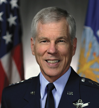 Shelton Space Commander
 Des Dorides for European GNSS Supervisory Agency