As we approach the halfway point of 2018, one cannot help but notice the amount of technology that we use every day and how it affects our daily lives. While George Jetson isn’t whizzing by in a flying car to his glass condo in the clouds, we are utilizing an incredible amount of technology in normal life.
I can sit here typing on a computer or tablet that is many times advanced than the first one I used in junior high school and think nothing of it as futuristic technology has become the norm.
The old standard joke about technology used to be about cell phones and television remote controls; if you needed to figure it out, get your child or even grandchild to help. The youngsters were the majority that could embrace technology because they didn’t have past methods to confuse their ability to figure out how to work the new device.
A funny thing has happened along the way, though; those kids are now grown, and technology has advanced even further.
To help explain the names and timeframes of our generations, I found this chart that explained it all:
| Generation Name | Births Start |
Births End |
Youngest Age Today* |
Oldest Age Today* |
| The Lost Generation – The Generation of 1914 |
1890 | 1915 | 103 | 128 |
| The Interbellum Generation | 1901 | 1913 | 105 | 117 |
| The Greatest Generation | 1910 | 1924 | 94 | 108 |
| The Silent Generation | 1925 | 1945 | 73 | 93 |
| Baby Boomer Generation | 1946 | 1964 | 54 | 72 |
| Generation X (Baby Bust) | 1965 | 1979 | 39 | 53 |
| Xennials – |
1975 | 1985 | 33 | 43 |
| Generation Y – The Millennials – Gen Next |
1980 | 1994 | 24 | 38 |
| iGen / Gen Z | 1995 | 2012 | 6 | 23 |
| Gen Alpha | 2013 | 2025 | 1 | 5 |
(Chart courtesy of Career Planner.)
To help put this chart in context, the average age of the professional surveyor in the United States is 59 and solidly in the Baby Boomer category. But even with an average that high, there are still a significant number of surveyors in the Silent Generation as the economic downturn of the late 2000s has forced them to continue well into their golden years.
HOW SURVEYORS FIT IN THIS DISCUSSION
The surveying profession has suffered through the same generational challenge as the rest of society. The younger set that started out surveying with electronics have now graduated to much more complex yet capable machinery. Prior to the mid- to late 1970s, electronic technology did not play a role in most surveying operations and tasks. The professional surveyor was widely considered a boundary expert, map maker and establisher of topographic data, with the high-tech mapping work left to the government geodesists (see my July 2017 Survey Scene column).
Most surveyors who learned their craft prior to the electronic age were trained on the job or obtained an engineering degree through a program that may have offered a limited surveying curriculum. Surveying was a career for the outdoor type and required traversing rough terrain at times, as well as being able to withstand weather extremes.
THE NON-TECHNOLOGY GENERATIONS
As a second-generation surveyor, I was fortunate enough to have been exposed to land surveying literally as it was performed by our forefathers. While the tasks performed didn’t utilize a true Gunter’s chain and compass, they were completed with a modern transit and steel tape. The surveys we completed didn’t require high tech equipment as our manual procedures greatly exceeded commonly accepted positional tolerances.

Most of the work performed by surveyors leading up to the early Baby Boomer generation was much simpler in theory but rarely easy to accomplish due to terrain, weather and the computations necessary to complete the boundary analysis. Traversing a parcel meant having a field crew of several people, often through brush and woods, and time consuming. A large parcel may be days or weeks of field to traverse around with most of it on foot. Once completed, the professional surveyor was tasked with often days of manual calculations, reduction of notes and determination of traverse closure. All the error from days of field work was then balanced through more hand calculations, usually by compass rule or transit rule, and hand drafted onto the final survey plat.
A similar story is followed with topographic and bathymetric surveys and creation of maps with existing conditions. Data collection performed to obtain locations and elevations of existing sites were by radial angle and distance or by grid method, with water depths being determined manually by use of lead lines. In the office this data is placed by manual drafting onto paper, sepia or vellum. Once elevations were plotted, contour intervals were determined by interpolation between each of these points. The creation of the contours was then drawn in by several methods, each with their own level of creativity by the drafter.
Because of the increased use and importance of electronic technology, data collection and advancements of the profession, today’s surveyor is faced with many more challenges than their predecessors. While the concepts for many tasks do follow the protocol for completing a multitude of survey duties, the way we go about collecting and analyzing the data is much more complex than in the past.
The need for our profession to identify these challenges and create opportunities for modern day surveyors is upon us, as our educational and training needs to be ramped up to stay current with demand. All professional surveyors, regardless of what generation they were born in, have filled or will fill an important role in society as expert measurers.
However, the rapid advancement of technology has exposed the lack of additional education and training necessary to keep our standing in serving the public’s health and welfare.
 My point here is not that the work and tasks performed by past generations of surveyors was easier, but it did require more manual labor and less technical education and training. I liken the situation to automotive mechanics and how much more technology goes into working on a modern car versus vehicles of earlier generations.
Many mechanics tuned engines by “feel” with no recordable technology to tell them otherwise. I wouldn’t think of calling the expertise shown by past mechanics as inferior to today’s automotive mechanics; each has been trained to rely on different skills sets to work with completely different engines. Thus, I feel the same way in comparing different generations of surveyors. Different tools and methods require unique and specific training for the surveyor to perform at the highest level.
For example, look at the survey-related equipment, software and services within GPS World magazine; most of the articles, case studies and advertisements are for things not even considered five to 10 years ago. All these items require a different mindset of more technical and analytical processing, so the surveyor’s educational requirements and approach must adjust with the technology.
As time marches forward, the need for more advanced surveyors is reaching a critical point.
HOW TODAY’S SURVEYORS GET THE JOB DONE
Today’s surveying profession, including the field and office technicians, rely heavily on technology more than ever.
Many threads of advancing technology go into weaving the tapestry of modern surveying, with the primary material of GNSS being utilized throughout. I have written in the past regarding my thoughts on the single greatest advancement in surveying (see my May 2016 Survey Scene column) and my argument gets stronger with newer technology adding to the way we measure our world.
Here are some of the tasks in which the surveying profession uses GNSS as a basis of measurement and location, and why specific education and training is critical to proper execution:
Boundary surveys
Like the surveyors before us, boundary establishment and re-establishment are the main responsibility of the profession. However, with GNSS, the ability to produce more location data has increased tremendously by reducing the need to perform intricate traverses through places when not necessary. It has also reduced the need to perform tedious traverse computations and adjustments; instead, least square adjustments are made to GNSS observational data to provide accurate results.
Topographic surveys
This data can be acquired by a combination of GNSS and conventional total station methods but is based upon geolocation information determined by primarily geodetic coordinates through GNSS solutions. Relying on GNSS data with no standard procedure for location and elevation verification can lead to major issues if not caught by an educated user.
Laser scanning / lidar / SLAM / photogrammetry / hyperspectral imaging
All these methodologies, also known as remote sensing, have revolutionized mass data collection with the enormous amounts of information that can be acquired in a short amount of time. Each has specific functionality and limitations but rely on geolocation as a main attribute of the data. Because of the large data files that are created, the output is in the form of a point cloud rather than the traditional P,N,E,Z,D format normally utilized by surveyors. Like topographic surveys, this data typically relies on GNSS information for geolocation.
Unmanned aerial and terrestrial systems
The newest of the data collection methodologies, the unmanned aerial vehicle (UAV) has taken the surveying world by storm. A good percentage of the new adopters (including me) utilize commercial grade multi-rotor units coupled with a high-resolution camera for orthometric photos and video clips of project sites.
While this method uses photogrammetry as its data collection method, it relies on GNSS for establishing ground control points (GCP) to establish geolocation to a known coordinate system. Higher end models incorporate RTK units to minimize the number of control points as well as utilizing lidar and/or hyperspectral modules for high end remote sensing.
Along with the airborne variety, land-based unmanned vehicles are starting to catch on as additional data collectors of open, navigable terrain. These autonomous devices are being equipped with lidar and cameras to augment aerial data in concert with UAVs to gather redundant information for quality checks.
As stated above, these remote sensing technologies, whether used statically or on an unmanned system, all create large point cloud data files that can be cumbersome to manage.
Bathymetric surveys
Many advancements have been made in producing measuring devices using sonar technology, including side- and multi-beam models for more detailed observations in varying conditions. GNSS plays a big role in this survey method due to the electronic ability to combine the depth readings of sonar instantaneously with geographic location. This improvement in data collection provides much more accurate and reliable information for the mapping of water bodies and passageways.
Bathymetric surveys are also getting in on the unmanned vehicle program as well with shallow draft autonomous watercraft being used in places where regular bathymetric vessels cannot go for survey data. More of these crafts are being implemented as they become more affordable.
What do these categories have in common? Most rely on specialized training and equipment to perform each specific task. Surveying has evolved past a “one size fits all” situation and demands that each sector of surveying have personnel trained for the job and have the right equipment to get it done.
A central figure in all these tasks is also GNSS technology; from survey-grade receivers to UAV’s, the tasks all revolve around geolocation.
HOW DOES THE PAST COEXIST WITH THE FUTURE?
The modern-day surveyor now has many different tools at their disposal that generations of surveyors before us couldn’t begin to fathom. The ability to perform at such levels of production and accuracy using new equipment and software is incredible and humbling. However, I’m afraid the technology is outpacing the profession. How many surveyors have taken the time to educate themselves on these enhancements? Because I think we are stretching ourselves too thin, now is the time for the professional surveying community to pause for a self-assessment of our abilities and what it will take to catch up with reality.
One of the biggest hurdles the surveying profession is facing are the lack of qualified technicians for positions both inside and out. The recession of 2008-2011 reduced the number of technicians in our field due to the lack of work being done in the economic downturn, but it also came at a time when technology was starting its upward run at increasing survey task efficiency. The downturn forced many surveyors and firms to make drastic cuts and reduce their investment in new technology, equipment and training to be more efficient. The surveying profession is now paying the price for that downturn with few adequately trained technicians along with licensed professionals not staying current with technological innovation and advances.
WHERE DO WE GO FROM HERE…?
The professional surveyor must embrace technology by promoting the profession to more places beyond the four-year college. We must start in junior-high and high school in math, science and history classes encouraging students to investigate surveying as a career. We also need to support technical and vocational programs that can help introduce surveying as a possible path beyond their certificate or associate degree. One of the simplest topics I use in presentations is the discussion of GNSS technology and how it is built into almost everything the student sees. From their cellphone to the cars their parent’s drive, GNSS surrounds us with geolocation information to make our lives easier.
These technicians aren’t going to all come from a four-year university programs; they are going to come from those teenagers who spend hours honing their hand-eye coordination with video games and drone racing. They will also be the fluid minds writing code for the next big app, and the surveying profession needs to embrace them to incorporate their work in our geolocation world.
The professional surveying occupation has become much more than establishing boundaries of parcels; it now requires knowledge for mapping literally anything in the world. The challenge now is to find those who want to help us continue this surveying and mapping tradition. Fellow surveyors: are you up to the challenge to find your replacement?


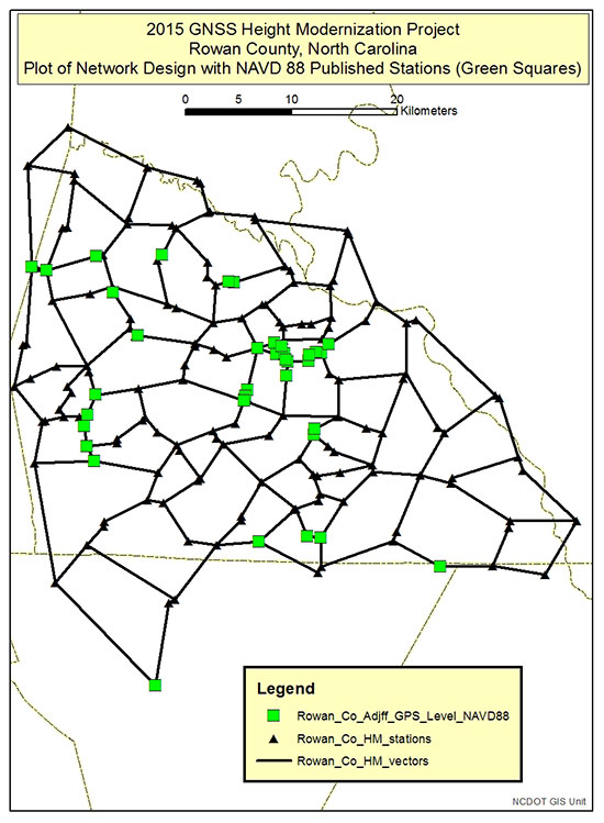
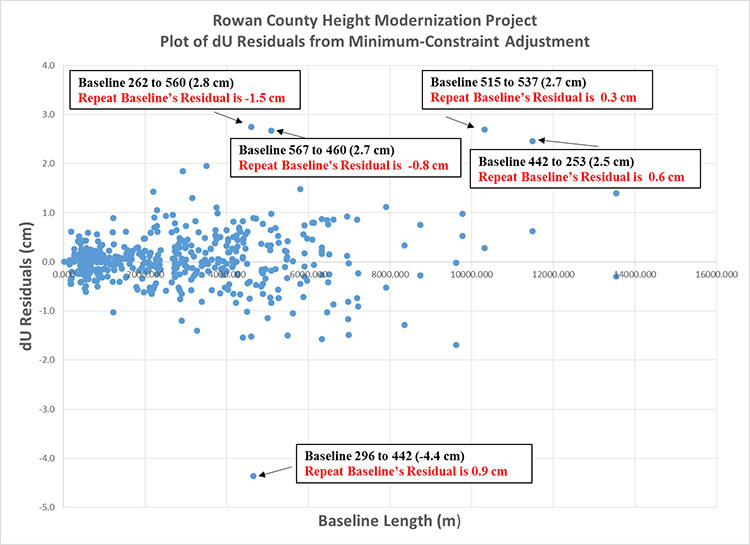
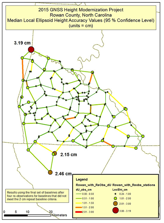
![Figure 1. [Figure 3 from Part 5] - Diagram depicting differences between GNSS-derived orthometric heights from a Minimum-Constraint Adjustment (using GEOID12B) and published NAVD 88 height values (units=cm).](https://stage.globalpositioningnews.com/wp-content/uploads/2016/04/Rowan-County_Newsletter_5_3.jpg)
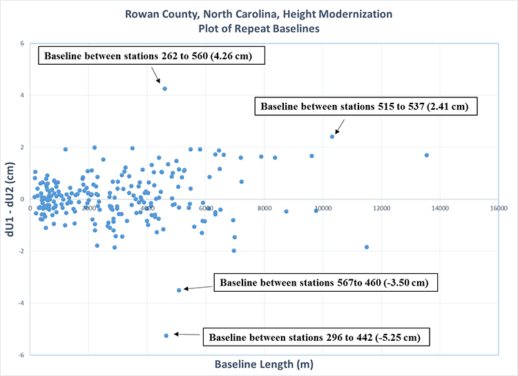
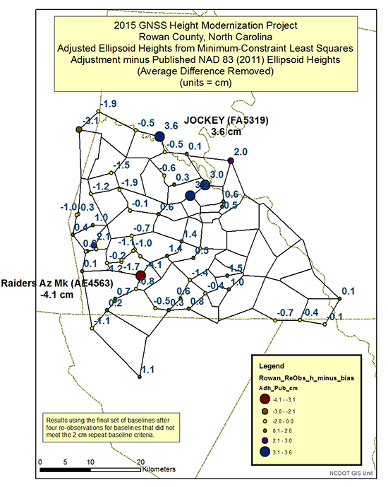
![Figure 2. [Figure 4 from Part 5] - Diagram depicting differences between GNSS-derived orthometric heights from a Minimum-Constraint Adjustment (using GEOID12B) and published NAVD 88 height values (units=cm).](https://stage.globalpositioningnews.com/wp-content/uploads/2016/04/Rowan-County_Newsletter_5_4.jpg)
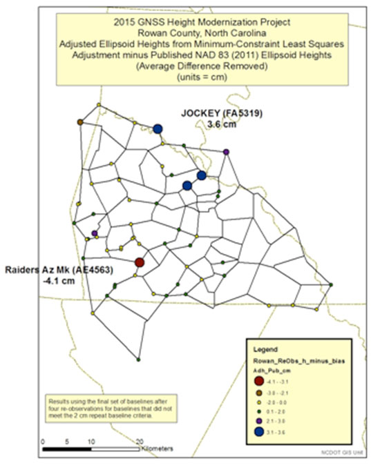
![Figure 3. [Figure 5 from Part 5] - Diagram depicting differences between GNSS-derived orthometric heights from a Minimum-Constraint Adjustment (using xGeoid15b) and published NAVD 88 height values (units=cm).](https://stage.globalpositioningnews.com/wp-content/uploads/2016/04/Rowan-County_Newsletter_5_5.jpg)
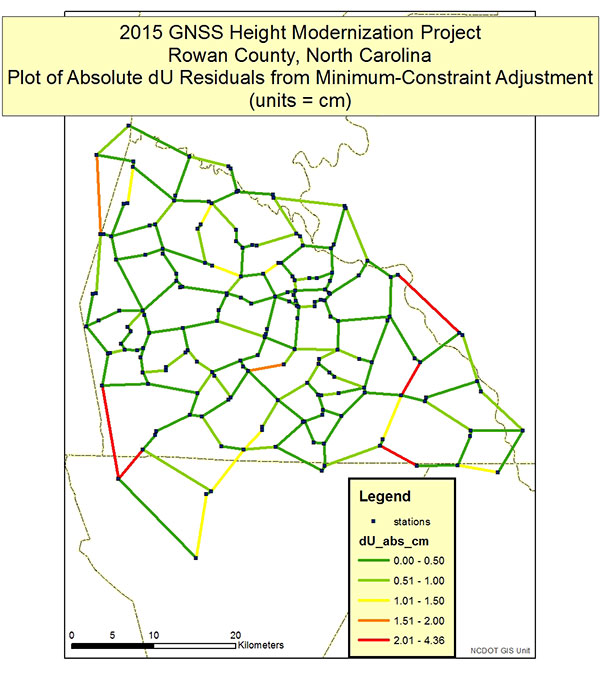
![Figure 4. [Figure 6 from Part 5] - Diagram depicting differences between GNSS-derived orthometric heights from a Minimum-Constraint Adjustment (using xGeoid15b) and published NAVD 88 height values (units=cm).](https://stage.globalpositioningnews.com/wp-content/uploads/2016/04/Rowan-County_Newsletter_5_6.jpg)