Topcon Positioning Group has added the FC-5000 to its line of data controllers for construction and surveying professionals. The 7-inch sunlight-readable display field controller is designed to provide operators a larger, more versatile and faster handheld computer for the modern construction site.
“At 7-inches, the FC-5000 has the largest handheld data controller screen in our product line,” said Ray Kerwin, director of global surveying products. “The display has a capacitive touch interface — with finger, glove, small tip stylus and water capable options — that is optically bonded to increase visibility. With the press of a key, a user can change the orientation of the screen from portrait to landscape to increase visibility when viewing maps or drawings.”
The controller is compatible with all Topcon GNSS receivers and total stations — operating MAGNET Field, Site and Layout software.
“The FC-5000 comes with two built-in cameras — an 8 MP camera with autofocus and LED flash for field photography — and a 2 MP camera on the front for video meetings. With 64GB of flash storage, users can store hundreds of photos in the unit, which can be easily transferred to any computer or USB stick,” Kerwin said.
Additional features include an optional 4G LTE cellular modem, internal GPS navigation, Bluetooth and Wi-Fi, and a battery life of 10-plus hours.
Basic procedures and tools for ensuring GNNS-derived orthometric heights meet the project’s desired accuracy
So far, this series of columns has addressed the following topics: basic concepts of GNSS-derived heights (Part 1), National Geodetic Survey’s (NGS) guidelines for establishing GNSS-derived ellipsoid heights (NGS 58) (Part 2), differences between hybrid and scientific geoid models (Part 3), and procedures and tools for detecting GNSS-derived ellipsoid height data outliers (Part 4).
These four columns were meant to provide the reader with basic concepts and procedures for estimating GNSS-derived ellipsoid heights and understanding hybrid and scientific geoid models. Now that the reader has a basic understanding of GNSS-derived ellipsoid heights and geoid models, this column will discuss procedures for estimating GNSS-derived orthometric heights.
Determining valid North American Vertical Datum of 1988 (NAVD 88) published heights is the most important process when using GNSS data and geoid models to estimate GNSS-derived orthometric heights. As mentioned in Part 4, NGS has developed procedures for estimating GPS-derived orthometric heights and these guidelines are documented in NOAA Technical Memorandum NOS NGS 59. The NGS 59 guidelines are separated into three basic rules, four control requirements, and five procedures that need to be adhered to for computing accurate NAVD 88 GNSS-derived orthometric heights. This column will address the NGS 59 guidelines and methods for evaluating the results of the GNSS project.
The three basic rules are fairly simple to understand and implement, provided that the reader has followed the previous columns in this series.
Three Basic Rules for Estimating GNSS-Derived Orthometric Heights:
Rule 1: Follow NGS 58 guidelines for establishing GNSS-derived ellipsoid heights when performing GNSS surveys (Parts 2 and 4 addressed this rule),
Rule 2: Use NGS’ latest National hybrid geoid model (such as GEOID12B) and latest experimental geoid model (such as xGeoid15B) — when computing GNSS-derived orthometric heights (Part 3 addressed this rule), and
Rule 3: Use the latest National Vertical Datum — for instance, NAVD 88 — height values to control the project’s adjusted heights (this column will address this rule).
The four basic control requirements are also simple, but, in certain regions of the country, may be difficult to implement.
Four Basic Control Requirements for Estimating GNSS-Derived Orthometric Heights:
Requirement 1: GNSS-occupy stations with valid NAVD 88 orthometric heights; stations should be evenly distributed throughout project.
Requirement 2: For project areas less than 20 km on a side, surround project with valid NAVD 88 benchmarks, i.e., minimum number of stations is four; one in each corner of project. [NOTE: The user may have to enlarge the project area to occupy enough benchmarks, even if the project area extends beyond the original area of interest.]
Requirement 3: For project areas greater than 20 km on a side, keep distances between valid GNSS-occupied NAVD 88 benchmarks to less than 20 km.
Requirement 4: For projects located in mountainous regions, occupy valid benchmarks at the base and summit of mountains, even if the distance is less than 20 km.
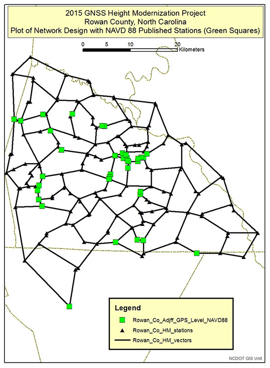
Figure 1 depicts the NCGS Rowan County Height Modernization project discussed in Part 4. Looking at Figure 1, there are stations with published leveling-derived NAVD 88 orthometric heights distributed throughout the project (requirement number 1).
What do I mean by published leveling-derived NAVD 88 orthometric heights? This is important to note because all NGS datasheets provide the NAVD 88 height with an attribute that describes what method was used to establish their height. The following is a list of attributes used on the NGS datasheet for NAVD 88 published heights:
There are various Vertical Control sources, as specified below:
ADJUSTED = Direct Digital Output from Least Squares Adjustment
of Precise Leveling. (Rounded to 3 decimal places.)
ADJ UNCH = Manually Entered (and NOT verified) Output of Least Squares Adjustment of Precise Leveling. (Rounded to 3 decimal places.)
POSTED = Pre-1991 Precise Leveling Adjusted to the NAVD 88 Network After Completion of the NAVD 88 General Adjustment of 1991. (Rounded to 3 decimal places.)
READJUST = Precise Leveling Readjusted as Required by Crustal Motion or Other Cause. (Rounded to 2 decimal places.)
N HEIGHT = Computed from Precise Leveling Connected at Only One Published Benchmark. (Rounded to 2 decimal places.)
RESET = Reset Computation of Precise Leveling. (Rounded to 2 decimal places.)
COMPUTED = Computed from Precise Leveling Using Non-rigorous Adjustment Technique. (Rounded to 2 decimal places.)
GPSCONLV = Leveled Orthometric Height tied to GPS HT_MOD Orthometric Height. (Rounded to 2 decimal places.)
LEVELING = Precise Leveling Performed by Horizontal Field Party. (Rounded to 2 decimal places.)
H LEVEL = Level between control points not connected to benchmark. (Rounded to 1 decimal places.)
GPS OBS = Computed from GPS Observations. (Rounded to 1 decimal places.)
VERT ANG = Computed from Vertical Angle Observations. (Rounded to 1 decimal place; If No Check, to 0 decimal places.)
SCALED = Scaled from a Topographic Map. (Rounded to 0 decimal places.)
U HEIGHT = Unvalidated height from precise leveling connected at only one NSRS point. (Rounded to 2 decimal places.)
VERTCON = The NAVD 88 height was computed by applying the VERTCON shift value to the NGVD 29 height. (Rounded to 0 decimal places.)
During the design of the survey, the user should first select as many stations with the attribute of ADJUSTED or LEVELING. If there aren’t any stations in a certain area of the project with the attribute of ADJUSTED or LEVELING, then stations labeled as GPS OBS with values rounded to 2 decimal places should be occupied. The other types of NAVD 88 heights aren’t accurate enough to validate your GNSS results.
Looking at Figure 1, there appears to be a few void areas in the north and east sections of the project. Although, it should be noted that the design meets the 20 km spacing rule (Rule number 3). Figure 2 depicts the NAVD 88 published heights for all leveling-derived stations and GPS-derived orthometric heights published to two decimal places (i.e., cm level). The published GPS-derived orthometric NAVD 88 heights filled in the void areas of the project. This is the practical reality of implementing the guidelines of NGS 59.
In some areas of the United States it may be difficult to locate enough valid NAVD 88 heights in the project’s area. First, let’s define a valid NAVD 88 height. Valid NAVD 88 height values include, but are not limited to, the following: control points which have not moved since their heights were last determined, were not misidentified, and are consistent with NAVD 88. This appears to be fairly simple, but it may be difficult for some users to determine if a station has moved since the height was last determined. In addition, in some areas of the country the user may not find valid NAVD 88 benchmarks every 20 km due to crustal movement. The user then may have to perform some classical precise leveling observations to evaluate the existing NAVD 88 heights and determine the relative accuracy of the geoid model in the areal extent of the project.
This doesn’t mean that the user must perform a leveling survey such that all GNSS stations are leveled to or even perform a large leveling network survey. The purpose of the leveling is to evaluate the geoid model and properly connect to the NAVD 88. Since each case is difference, i.e., NAVD 88 height problems and geoid accuracy will vary in each region of the country, as well as each individual project accuracy requirement will be different, it is impossible to describe exactly what the user will have to do. NGS will, however, assist users when they’re planning their surveys. You can contact a NGS advisor through their Regional Advisor Program.
The five basic procedures for estimating GNSS-derived orthometric heights may appear to users to be the most complex and most difficult to understand. However, as users perform more GNSS surveys and discuss their results with others, they seem to quickly understand why these procedures are needed.
Five Basic Procedures for Estimating GNSS-Derived Orthometric Heights:
Procedure 1: Perform a 3-D minimum-constraint least squares adjustment of the GNSS survey project, i.e., constrain one latitude, one longitude, and one orthometric height value. This procedure was described in Part 4.
. Procedure 2: Using the results from the adjustment in procedure 1, detect and remove all data outliers. (NOTE: If the user follows NGS’ guidelines for establishing GNSS-derived ellipsoid heights (NGS 58), the user will already know which vectors may need to be rejected and following the GNSS-derived ellipsoid height guidelines should have already re-observed those base lines.)
The user should repeat procedures 1 and 2 until all data outliers are removed.
Procedure 3: Compute the differences between the set of GNSS-derived orthometric heights from the minimum constraint adjustment (using the latest National geoid model, for example GEOID12B, and National experimental geoid model, for example xGeoid15B) from procedure 2 above and the corresponding published NAVD 88 benchmarks.
Procedure 4: Using the results from procedure 3, determine which benchmarks have valid NAVD 88 height values. This is the most important step of the process. Determining which benchmarks have valid heights is critical to computing accurate GNSS-derived orthometric heights. (NOTE: The user should include a few extra NAVD 88 benchmarks in case some are inconsistent, i.e., are not valid NAVD 88 height values.)
Procedure 5: Using the results from procedure 4, perform a constrained adjustment holding one latitude value, one longitude value, and all valid NAVD 88 height values fixed.
As mentioned in Part 4, during the analysis of the GNSS-derived ellipsoid heights, the user needed to perform a minimum-constraint least squares adjustment and look for outliers. This ensures that the GNSS-derived ellipsoid heights meet the user’s desired standards. Now, the user must ensure that the NAVD 88 heights that are going to be used to control the final set of GNSS observations and geoid heights are valid.
Part 4 described in detail how to analyze the project’s ellipsoid heights. If the user followed the procedures outlined in Part 4, then procedures 1 and 2 were performed.
The techniques described below are meant to be fairly simple for users to implement. They are not rigorous and are not the only way to detect outliers. They will, however, assist the user in determining which NAVD 88 benchmarks are valid. Procedure 3 is simply computing the GNSS-derived orthometric heights and comparing the results with the published leveling-derived NAVD 88 heights. The set of GNSS-derived orthometric heights are obtained by performing procedure 1. Figures 3 and 4 provide the differences between the GNSS-derived orthometric heights using GEOID12B and published leveling-derived NAVD 88 orthometric heights. (NOTE: One station’s latitude, longitude, and orthometric height (Buffalo 2) was constrained in the minimum-constraint least squares adjustment. Since any of the stations with a published height could have been constrained in a minimum-constraint least squares adjustment, an average difference (a bias) computed using all of the differences was removed from each difference.)
All relative height differences between adjacent station pairs should agree within 2 cm for 2-cm surveys and 5 cm for 5-cm surveys to be considered valid NAVD 88 benchmarks. Relative height differences that do not meet this guideline should be investigated.
Part 3 discussed the difference between hybrid and scientific geoid models and that the user should use both models during their analysis of GNSS surveys. As mentioned above, Figures 3 and 4 provided the difference using GEOID12B; Figures 5 and 6 provide the differences using xGeoid15b. Tables 1 and 2 provide this information in tabular form.
Table 1. Differences between GNSS-derived orthometric heights from a minimum-constraint adjustment (using GEOID12B) and published NAVD 88 heights (GEOID12B results sorted and highlighted).Table 2. Differences between GNSS-derived orthometric heights from a minimum-constraint adjustment (using xGeoid15b) and published NAVD 88 heights (xGeoid15b results sorted and highlighted).
The reader should note that most differences in Figure 3 are less than 2 cm, but there is a several differences greater than +/- 2cm. Eight stations have differences greater than +/- 2 cm [see Table 1, column labeled “GNSS-Derived Orthometric Height (using GEOID12B) minus Published NAVD 88 Height (cm)”]. These stations should be investigated as a potential outliers.
Looking at Figure 3, the reader should notice that several stations less than 20 km apart have a relative differences greater than 4 cm.
For example, the following three station pairs have large relative height differences: [Buffalo 2 (AB6805) – Phaniel (AB6836): 4.9 cm], [V 49 (FA0151) – Phaniel: 5.6 cm], and [Row 9 (DG5715) – Phaniel: 5.7 cm]. To investigate this further, we need to introduce the scientific geoid model in the analysis. Figures 5 and 6 are plots of the differences using xGeoid15b. The user should notice that the relative differences using the scientific geoid model (Figure 5) between the same stations pairs are all less than the differences using GEOID12B (Figure 3).
For example, the relative differences between Phaniel and Buffalo 2 is 4.9 cm [(2.8 – (-2.1)] using the GEOID 12B geoid model. The relative differences between the same two stations using xGeoid15b is only 0.7 cm [4.2 – 3.5]. This implies that the hybrid geoid model may have been distorted to agree with stations that may have moved since the last time they were observed. This could be an indication that station Phaniel and/or Buffalo 2 may have moved since they were last surveyed. If so, once again, they should not be constrained in the final adjustment.
It should also be noted that only five stations have differences greater than +/- 2 cm using xGeoid15b [see Table 2, columns labeled “GNSS-Derived Orthometric Height (using xGeoid15b) minus Published NAVD 88 Height (cm)”]. However, the five outliers are significantly larger than the rest of the differences (see highlighed section on Table 2). All other differences using xGeoid15b are less than +/- 1.7 cm. These five leveling-derived heights should be investigated for possible movement before constraining their heights in the final adjustment.
As previously mentioned, looking at Figures 5 and 6, stations Phaniel and Buffalo 2 seem inconsistent with the other stations in the southern half of the project. Another potential outlier highlighted in Table 2 is station Row 3 with a difference of -3.8 cm. These stations should definitely be investigated for potential movement.
When performing constrained GNSS-derived orthometric height adjustments, it is important to determine the effect of the constraints on the adjusted heights of the unconstrained stations. If a station’s published height is not valid, then constraining that value could distort the final set of adjusted coordinates. Users should compare the differences between the adjusted heights from the constrained adjustment with the adjusted heights from the minimum-constraint adjustment. Figures 7 and 8 are plots that depict the differences between the adjusted heights obtained from a fully constrained adjustment (using GEOID12B) and a minimum-constraint adjustment.
Looking at Figures 7 and 8, the reader should notice that several of the heights of stations in the southern portion of the network have changed by more than 3 cm. More importantly, some of the closely spaced stations have large differences in relative height changes. For example, the adjusted height at station Phaniel changed -4.9 cm (this station was constrained) and its neighbor station Moose (4 km from Phaniel) only changed -3.1 cm. This means the constraint changed the height difference between Phaniel and Moose by 1.8 cm. If the constraint is valid, then the user should use it in the constrained adjustment. However, during our analysis of this project, we identified station Phaniel as a potential outlier which means that station Phaniel may have moved since it was last surveyed. As previously mentioned, if a station moved since it was last surveyed it should not be constrained because it may distort the adjusted heights around it. Saying that, it is important to maintain consistency in a National Vertical Control Network, e.g., NAVD 88, when incorporating survey data into the network. If the station is not constrained and it did not move since it was last surveyed, then all stations surrounding the superceded station will be inconsistent with its neighbors. Therefore, if a user cannot determine that the station has moved since it was last surveyed, it should be constrained in the final adjustment.
To determine the effect of constraining station Phaniel, another constrained adjustment was performed constraining all published NAVD 88 leveling-derived orthometric heights except for station Phaniel. Figures 9 and 10 are plots that depict the differences in adjusted heights due to constraining all published NAVD 88 leveling-derived orthometric heights except for station Phaniel. The plots indicate that by not constraining Phaniel, the changes in adjusted heights due to that constraint were all reduced. All differences in the area of station Phaniel are less than 3 cm and the relative height changes have been significantly reduced. For example, the relative height change involving station Phaniel and Moose was reduced from -1.8 cm [-4.9 – (-3.1)] to -0.2 cm [-1.9 – (-1.7)], and from station Phaniel to Cold, the relative height change decreased from -2.9 cm [-4.9 – (-2.0)] to -0.6 cm [-1.9 – (-1.3)]. (See Figures 8 and 10.) This is a reason why it is very important to determine if a station’s published height is still a valid NAVD 88 height.
This column discussed procedures for estimating GNSS-derived orthometric heights following NGS 59 guidelines. It provided methods for evaluating the results of the project and identifying stations with valid NAVD 88 published heights. More analysis needs to be performed to identify all the valid stations to be constrained in this project. In the next column, we will continue to analyze the changes in adjusted heights due to different constraints, compare the results to the published NAVD 88 GNSS-derived orthometric heights observed in this project, and investigate the leveling network used to establish the published NAVD 88 leveling-derived orthometric heights.
Sokkia has introduced the latest addition to its line of field controllers for use with construction and surveying applications, the SHC5000. Operating MAGNET Field, Site and Layout software, the newest field controller is designed to provide a more versatile and faster handheld computer for GNSS receivers and total stations, with the largest screen size in the Sokkia line.
“The SHC5000 boasts a 7-inch sunlight-viewable screen, which makes it the largest in our line of field controllers,” said Ray Kerwin, director of global surveying products. “The display’s capacitive touch interface comes with finger, glove, small tip stylus and water capable options. Operators can change the screen from portrait to landscape when viewing maps or drawings, depending on which orientation is preferable.”
The SHC5000 comes with two built-in cameras. One uses an 8 MP camera with autofocus and LED flash that is designed for uses such as field photography. The second has a 2 MP camera on the front side of the unit for purposes such as video meetings.
Additional features include 64 GB of flash storage, an optional 4G LTE cellular modem, internal GPS navigation, Bluetooth and Wi-Fi, and a battery life of 10-plus hours.
The membership of the Open Geospatial Consortium (OGC) seeks public comment on its candidate OGC Land and Infrastructure Conceptual Model Standard (LandInfra). Deadline for comments is March 2.
LandInfra defines concepts for land and civil engineering infrastructure facilities.This conceptual standard will provide a basis for one or more implementation standards for encoding infrastructure data. Developers will use the encoding standard to implement software and services that enable users of diverse technologies and vendor platforms to efficiently exchange information about land and civil engineering infrastructure facilities.
The extended stakeholder community for this standard spans civil engineering (such as road and rail) and surveying; land parcel; facility and asset management; and government information communities. It is applicable throughout the entire facility lifecycle, including planning, design, construction, operations, maintenance, and removal. It represents a seminal venture into GIS-CAD-BIM integration.
After evaluating the LandXML 1.2 schema, the OGC Land and Infrastructure Domain Working Group (LandInfraDWG) recommended the development of an alternative standard to be part of the OGC standards baseline. With shared interest by the buildingSMART International Infrastructure Room, it was agreed that this would be a concepts-only document — encodings such as GML, IFC, and possibly others would follow as separate implementation standardization efforts. An anticipated GML encoding will be compatible with other GML standards such as CityGML. Having a common underlying Conceptual Model across all LandInfra encodings will help ensure compatibility across multiple encoding standards.
The OGC is an international consortium of more than 515 companies, government agencies, research organizations, and universities participating in a consensus process to develop publicly available geospatial standards. OGC standards support interoperable solutions that “geo-enable” the web, wireless and location-based services, and mainstream IT. OGC standards empower technology developers to make geospatial information and services accessible and useful with any application that needs to be geospatially enabled.
Topcon Positioning Group has released the latest addition to its ES total station series, the ES-50. Featuring advanced reflectorless capabilities, the new ES-50 is designed to provide an entry-level total station option with a fast and powerful electronic distance meter (EDM).
“With the functionality of many high-end robotic total stations, our ES series is known to be full-featured and ready to tackle modern job sites,” said Ray Kerwin, director of global surveying products. “The ES-50 incorporates all those time-honored expectations, along with a reflectorless EDM of up to 350 meters, and 4,000 meters with the use of a prism.”
The ES-50 offers 2- and 5-arc second accuracies for distance measurements in projects such as land surveying, topography and as-built, construction and layout, or foundation and exterior job sites.
Additional features include a battery life of up to 15 hours, dual-axis compensation, a waterproof design and a laser pointer.
Windows 10 and a new large display are key features of Juniper Systems’ latest tablet, Mesa 2 Rugged Tablet, released today.
Juniper Systems is a provider of ultra-rugged field data collection solutions.
Featuring the largest display produced by Juniper Systems to date, the Mesa 2 is also Juniper Systems’ first handheld to run on the new Windows 10, which the company said allows for improved decision-making in the field, as well as smooth transitioning from field data collection to office work and back.
With a full Windows 10 operating system, the Mesa 2 provides users with access to a broader range of software options to meet their data collection needs and is powerful enough to use in place of a desktop computer when in the office. The Mesa 2’s 7-inch display strikes a perfect balance between providing ample viewing area for collected data and reducing overall weight for minimal fatigue and superior, all-day comfort, the company said.
The Mesa 2 is designed to perform reliably in harsh environments, and is the only IP68-rated rugged Windows tablet available, providing complete protection against water and dust. It maintains a seal while its ports are in use, while most other tablets on the market are exposed to damage from water and dust if the port cover is not securely in place.
The Mesa 2 also features an extraordinary IllumiView display, providing best-in-class visibility in any lighting conditions, and its chemically-strengthened Dragontrail glass touch screen provides superior durability, reducing haze from surface scratches and cracks normally caused by accidental impact.
The Mesa 2 battery provides users with a full 8-10 hours of runtime, allowing for maximum productivity throughout the workday. Users may also purchase an optional expansion battery from Juniper Systems that provides an additional 4-5 hours of runtime plus hot swap capabilities for those extra-long days where overtime is required.
“The Mesa 2 is in a new sphere relative to our other ultra-rugged devices,” said Nate Holman, Director of Sales and Marketing at Juniper Systems. “While it features the same degree of outstanding quality and ruggedness as other Juniper products, the Mesa 2 provides users with more software options and greater processing capabilities, due to its full Windows 10 operating system and Intel quad-core processor. The Mesa 2 is designed to improve productivity along every point of the data collection process, from the initial planning and gathering of data, to the later data analysis, and finally through the decision-making process. It’s a tablet optimized for efficiency, designed to be ‘your office, anywhere’.”
The Mesa 2 Rugged Tablet will begin shipping in the first quarter of 2016.
High-tech aerial laser surveying is being employed to reveal the hidden archaeology of an Iron-Age hill settlement in Lancashire, England.
Visually, the archaeological features are difficult to see, but a Bluesky laser survey, commissioned by the Morecambe Bay Partnership, is expected to reveal previously undiscovered details of a settlement at Warton Crag. Identified as an important Heritage at Risk site, the site has already been subject to low-level archaeological investigations, which have identified remains from a small, well defended hill fort.
“It is imperative that we get a better definition of the archaeological remains that are currently ‘hidden’ by the dense vegetation cover,” said Louise Martin, H2H cultural heritage officer at the Morecambe Bay Partnership. “This will enable us to develop conservation strategies for the site and work towards reducing the risk to the archaeological remains. The site is currently on Historic England’s ‘at risk’ register, so this work is crucial in developing partnerships and strategies to protect the monument for future generations.”
The Bluesky lidar system uses lasers to accurately measure the earth’s terrain and record features on the ground in 3D. A dedicated survey plane is equipped with aerial photography equipment and will fly over the site during the winter months when the tree and canopy cover is at its minimum.
Bluesky will process the millions of individual laser measurements to create detailed 3D computer models of the Earth’s relief — a Digital Terrain Model (DTM) — and ground surface including buildings and vegetation — a Digital Surface Model (DSM). This will allow the Morecambe Bay Partnership to model scenarios and strategies and share information with project partners.
Geneq has introduced a new “all-in-one” GPS, GNSS and RTK Data Collector Series, the SXPro.
The professional-grade series of handheld receivers is accurate, rugged and competitively priced, the company said.
Standard features include an extra-long battery life of more than 10 hours on a charge as well as a large outdoor-viewable touchscreen. The handhelds are rated IP65 for protection against water and dust.
The SXPro handheld is also equipped with a 5-megapixel autofocus camera and Microsoft utilities. The SXPro is sold as a fully loaded package that includes a spare battery, hard carrying case and Field Genius Survey Data Collection software.
The SXPro series is built for mobile survey and GIS users for applications such as water, electric and gas utilities; transportation; mining; agriculture; and forestry.
The SXPro RTK (real-time kinematic) model offers 220 multi-constellation channels for centimeter accuracy with RTK networks. A surveyor-grade external dual-frequency antenna and cables are included.
The SXPro GNSS offers 372 multi-constellation channels for sub-meter accuracy with SBAS corrections.
The UB380 GPS/GLN/BDS tri-constellation octa-frequency high-precision board.
High-end GNSS board
For high-precision positioning, navigation and GBAS applications
The UB380 multi-GNSS receiver has 384 channels, based on Unicore’s multi-GNSS system on a chip. It features Unicore’s latest real-time kinematic (RTK) engine, which can process triple-frequency BDS and GPS and dual-frequency GLONASS observation data. This can significantly reduce initialization time, improve position accuracy and enhance reliability in difficult environments such as city canyon and canopy, as well as make the long baseline RTK possible. The receiver board can support GPS L1, L2 and L5; GLONASS L1, L2; and BDS B1, B2 and B3. The support of GPS L2P and L2C can satisfy the high-precision requirements of GBAS reference station equipment. The UB380 is compatible with industry-standard GNSS boards in size, interfaces and electrical standards.
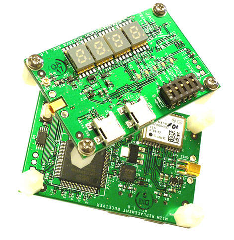
M12M Replacement Receiver GNSS module. Photo: Jackson Labs Technologies
Legacy receiver module
Plug-and-play upgrade for xli server, fury GPSDO
The M12M Replacement Receiver released is form, fit and function compatible to the legacy Motorola M12M and M12+ timing and navigation receivers. It uses an eighth-generation GNSS timing-enabled receiver, allowing 72 GNSS-channel reception with any two GNSS systems being received simultaneously. It adds configurability via USB ports and dual in-line package (DIP) switches and various status displays. GPS, GLONASS, BeiDou, QZSS and SBAS signals can be received. The module supports NMEA, Motorola binary and u-blox binary as well as SCPI (GPIB) communication protocols; is designed to allow plug-and-play retrofit of equipment designed for legacy Motorola receivers; and is certified as a plug-and-play upgrade to the Symmetricom/Microsemi XLI server and the Jackson Labs Technologies Fury GPSDO. It can be used to retrofit products for GLONASS/BeiDou compatibility. The module enhances performance parameters such as time to first fix; position, velocity and timing accuracy; tracking sensitivity; the addition of SBAS (differential compensation) capability; and the addition of external interfaces such as USB and a synthesized frequency output.
High-gain, high-rejection family designed for cell and telecom
The TW3150/52 antennas feature a 50-dB low-noise amplifier (LNA) gain to handle long cable runs often associated with installation on telecommunications towers. They cover the GPS L1 and SBAS (WAAS, EGNOS and MSAS) frequency bands and provide excellent cross-polarization rejection and enhanced multipath rejection.The TW3150 antenna features a four-stage dual-filtered LNA, while the TW3152 antenna includes an additional SAW pre-filter. This provides better than 80-dB of signal rejection above 1610 MHz and below 1545 MHz. The antennas are IP67 and MIL-STD-801F Section 509.4 compliant to withstand challenging environmental conditions.
Provides support for GPS, GLONASS and BeiDou with MediaTek
The ORG1510-MK Multi Micro Hornet is a fully integrated multi-GNSS (GPS, GLONASS and BeiDou) module. The miniature low-power architecture is designed to provide a GNSS component to devices that require fully featured components with small footprints, such as UAVs designed to follow action sports and other fast-moving activities or wearables. The ORG1510-MK contains the MediaTek MT3333 chip, which supports a fast update position calculation rate, and contains an onboard flash memory that does not erase when power is off. It consumes little power with the use of both standby mode and backup mode, and, in advanced applications, a periodic mode that can turn the device on and off when in backup or standby.
Designed for recording sports activities, the FLYPRO XEagle UAV has replaced traditional UAV remote controllers with the XWatch, a smartwatch designed to control the XEagle. Users can control the devices to take off, land and follow, as well as adjust flight height with one click on the wrist within 300 meters. The smartwatch design enables users to fly the aerial vehicles to take high-definition pictures and videos while engaging in intense sports. A voice-control feature allows users to fly the XEagle without moving their hands using commands such as “FLYPRO, take off” and “FLYPRO, follow me”.
Thermal imaging camera core designed for integration
FLIR Tau 2 thermal imaging cameras are suited for demanding applications like UAVs, thermal weapon sights and handheld imagers. Improved electronics now give Tau 2 even more capabilities, including radiometry, increased sensitivity (<30 mK), 640/60 Hz frame rates, and powerful image processing modes that dramatically improve detail and contrast. Since the electrical functions are common between the Tau 2 640, 336 and 324, integrators have direct compatibility between the different camera formats, and Tau camera versions share many of the same lens options.
Amazon’s latest version is designed to deliver packages in 30 minutes
Source: Amazon
A new drone design introduced by Amazon for its planned Prime Air Delivery service is larger than the previous quadcopter and has a more advanced design, including the ability to operate with an auto-loading system that sets the payload inside an internal carrier bay. The hybrid design combines vertical lift and horizontal flight capabilities using lift fans and a pusher prop. The drone is capable of flying at an altitude of about 400 feet (122 meters) at about 55 mph (88 km/h) for a range of 15 miles (24 kilometers). It has sense-and-avoid situational awareness technology and is designed to deliver small packages in under 30 minutes.
The M300 Pro is a multi-purpose CORS GNSS receiver designed for applications such as positioning infrastructure, active geodetic network, deformation monitoring, machine guidance, harbor construction, land surveying and marine surveying. Designed for reference stations, the M300 Pro tracks GPS, GLONASS and BeiDou (B1, B2, B3), and will track Galileo, QZSS and other coming constellations. Its web server function enables remote control for access, configuration, programming, data download, reboot/restart, firmware update and code registration. It is compatible with many kinds of CORS software, using the standard data format RTCM and the various data transfer protocols such as UDP, TCP and NTRIP. Raw GNSS observation data can be saved in RINEX format and remotely downloaded. Multiple ports can be configured and connected with external sensors such as meteorological sensors, barographs and inclinometers. The PPS output function provides a guarantee for precision timing. It also has the functionality of event mark and external memory.
The Leica Velocity and Displacement Autonomous Solution Engine (VADASE) detects fast movements of man-made and natural structures in real time, running on board Leica reference stations and monitoring receivers. VADASE provides an in-depth look at accurate, high-rate velocity and displacement information of various activities and structures. It gives engineers and researchers complete, precise and reliable monitoring information. VADASE delivers actionable information independent of any GNSS real-time kinematic (RTK) correction service.
GNSS receiver with onboard memory for data storage
The DELTA-3 receiver has 864 GNSS channels, along with three powerful processors and program memory in a single chip, which uses less power and makes the total system less expensive. The 864 channels allow tracking of all current and future satellite signals. Delta-3 can track and decode the QZSS LEX signal messages. It is a powerful and reliable receiver for high-precision navigation systems, including high-dynamic systems, for machine and traffic control, high-precision surveying, and geodynamics and aerogeophysics applications. Delta-3 can operate as a receiver for post-processing, as a Continuously Operating Reference Station (CORS), or as a portable base station for real-time kinematic (RTK) applications, and as a scientific station collecting information for special studies such as ionosphere monitoring.
A configuration of ArcGIS and a JavaScript application
Photo Survey is designed for local governments to publish street-level photo collections and conduct focused property surveys that can identify blight, damaged structures or construction activity. It leverages location-enabled photos produced by many commercially available cameras and simplifies data processing so street-level photo collections can be gathered on a regular basis. Photo collections can then be combined with relevant survey questions in an ArcGIS Online map, and shared with the Photo Survey application. Once complete, the Photo Survey application can be used by the general public or local government staff to review street-level photos and complete property surveys.
Integration for infrastructure monitoring, navigation
By Desislava Staykova and Nico Zill
Rapid development in the technology of combined sensors within complex systems has taken place over the last decade. Such systems provide different accuracy levels, offering the possibility of use in application areas such as surveying, railway and automotive engineering, land administration, and for navigation purposes.
Multi-sensor integration and fusion is a comprehensive process of reading and combining sensor signals to ensure a higher level of data reliability and accuracy. Input data from every sensor and further combination with specially developed algorithms ensures the complete identification of observed features, which would be impossible with data from each individual sensor operating separately.
Because of its flexibility and the possibility for fast and continuous data measurement, multi-sensor integration and fusion has evolved rapidly in different areas. The object of this article is to overview the use of high-end and low-cost system complexes and software solutions for the purposes of the engineering geodesy, transportation and navigation.
Deformation Monitoring
Geodetic measurements for monitoring and displacements analysis of various engineering objects have always played an important role in maintaining structures like bridges, dam walls, building columns, wind power generators, and other construction.
This requires properly designed network schemes enabling continuous and highly accurate measurements. For such angular and length measurements of millimeter-level accuracy that must be performed in intervals of minutes, hours or a day, standard total stations are being replaced by automated ones (ATS) comprising precise servomotors, automatic target recognition sensors, electronic inclinometers, self-calibration control systems and other sensors.
The synchronized process of high-accuracy measurements (angular accuracy better than one second and distance accuracy better than one millimeter) and simultaneously adjustment software enables real-time or post-processing deformation monitoring and analysis. This type of hardware and software combination is often used during the life cycle of a project for construction and reconstruction of objects and for regular monitoring of the object’s stability.
Terrestrial Laser Scanning. The need for precise modeling and geometrical characterization of large structures and open areas as dams, mines, landslides and others cannot be covered by traditional surveying methods which require the use a huge number of points for describing the object’s surface. The development of laser scanning technology in the last decade offers a new way for deformations measurements and becomes part of the infrastructure monitoring.
The high scanning speed, dense measurement of huge numbers of points and high accuracy gives terrestrial laser scanning (TLS) an advantage other technologies used for large structural monitoring. Compared with the technologies using single point monitoring approaches where the displacements detection is limiteded to specific benchmarks, TLS provides high data redundancy. Combined with proper software products, this technique offers the possibility for high-accuracy surface modeling and displacement detection at the millimeter level. The scanned object consists of a large number of points, which allows implementation of mathematical algorithms for modeling and analyzing the object’s behavior.
Another advantage of TLS as a remote sensing measurement tool is the minimized impact of the operator over the observed points and network.
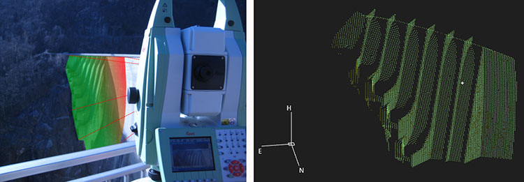
A new method for structural monitoring has emerged recently, comprising the advantages of the TLS, GNSS, geotechnical and meteo-sensors, enabling wide-area coverage and surface monitoring. One such tool is shown in Figure 1.
Figure 1. Terrestrial laser scanning combined with GNSS and other sensors enables wide-area coverage and survace monitoring. (Images courtesy of Leica Geosystems)
Mobile Laser Scanning
For different navigation purposes, for monitoring and investigation of wide areas, static measuring methods are being replaced by complex mobile measuring combinations of both high-end and low-cost sensors, to ensure fast, continuous and accurate data acquisition.
Recently mobile laser scanning (MLS) has experienced rapid development and proved its usage particularly in the railway and automotive sectors, for deformation analysis, for monitoring and documentation of as-built street and railway networks and the corresponding infrastructure objects.
MLS for Rail and Road. The advantages of MLS for fast, high-accuracy and complete scanning of the surroundings make it an important part of current railway and road conditions monitoring.
Continuous data acquisition and processing minimizes operator errors, and significantly reduces the time for performance of the surveying work and a-posteriori data analysis.
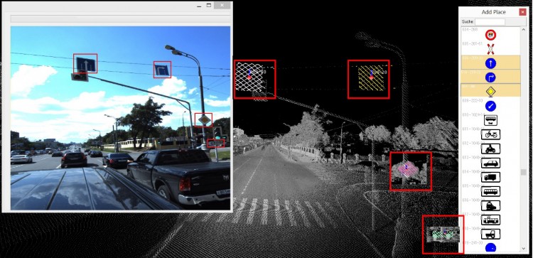
Localization and recognition of infrastructure objects forming part of railway and road environment has long been of primary importance in the transportation sector.
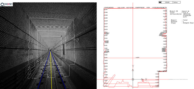
For determination and documentation of as-built railway and street networks from acquired data, Technet-Rail (Berlin, Germany) developed two software solutions, SiRailScan and SiRoadScan, for point-cloud analysis. The integrated mathematical algorithms ensure high-accuracy extraction and adjustment of the as-built left rail, right rail and center line, as well as of the roads’ border lines.
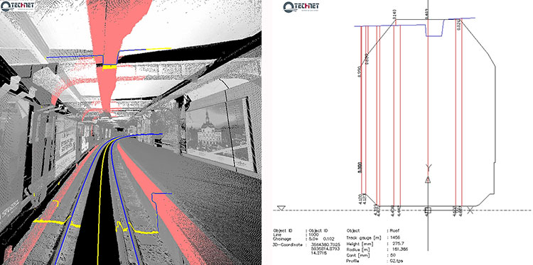
The adjusted geometry forms the basis for driving speed control tests, determination of the as-built environment for clearance detection and documentation, investigation of catenary wire deviations, ballast and road settlements, traffic signal positions, and any changes in the existing situation (see Figures 2 and 3).
Figure 2. Adjusted as-built rail geometry with SiRailScan used as basis for performance of clearance analysis and documentation in chainage based railway system.Figure 3. Adjusted with SiRoadScan road border lines. Detection and recognition of the roads signals.
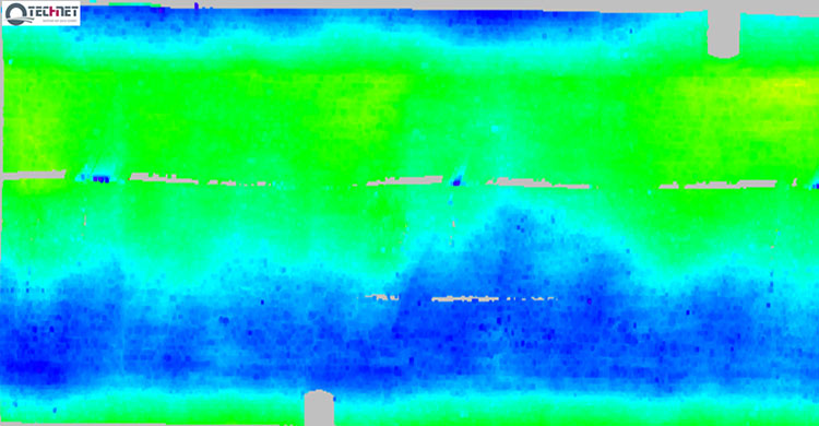
In response to the growing interest in application of the MLS technique and a-posteriori data adjustment for monitoring purposes, Technet-Rail developed additional tools for deformation analysis of structures such as tunnel bodies, railway bridges and road surfaces. The integrated software solutions enable comparison between the designed and as-built situation, epoch-wise analysis, modeling of the structure, development into 2D followed by color-coded deformation map (see Figures 4 and 5).
Figure 4. Tunnel deformation analysis performed with SiRailScan based on the as-built rail geometry. Automated calculation of differences between designed and as-built tunnel structure.Figure 5. Tunnel deformation analysis with SiRailScan based on a pre-defined form and direction.
MLS for Navigation. Multi-sensor integration is the basis for operation of the moving measuring systems integrating hardware devices such as laser scanning devices, GNSS, inertial measurement units (IMU), distance measuring instruments (DMI) and specific software algorithms for data synchronization. A milestone in the development of such systems is the measurement and navigation in indoor places or in areas with low or no GNSS coverage.
The need for safe and reliable navigation in transportation systems such as train control systems, intelligent vehicle systems, system tracking, in urban environments, underground areas, and other areas with no available GNSS signal stimulated much research in the area of multi-sensor integration and fusion. the main scope of some studies is the integration of different sensors delivering information for the attitude, velocity, acceleration such as the IMUs, inclinometers, wheel sensors, and correspondent filtering algorithms to achieve the best possible position accuracy without usage of GNSS signals.
Conclusion
For decades, infrastructure objects such as dam walls, bridges, tunnels, roads and railway tracks form a substantial part of civil engineering and engineering geodesy. The integrity of their structure requires deep knowledge of the behavior of these objects and the various methods for their optimal and high accurate monitoring. The rapid development evolution of multi sensor integration in combination with laser scanning technology makes it an essential method for accurate, continuous and dense measurement for the purposes of the engineering surveys.
Desislava Staykova and Nico Zill are engineers with Technet-rail 2010 GmbH, Berlin, Germany.
MicroSurvey Software has released MicroSurvey CAD 2016, the newest generation of its desktop survey and design program for land surveyors and civil engineers. Powered by a new IntelliCAD 8.1a engine and enhanced with a suite of new point-cloud management tools, the software makes high-impact drafting and design fast and intuitive, the company said.
Users on multi-core computers will experience up to 300 percent faster performance compared to previous versions, which substantially improves productivity. Navigation has been enhanced through a new ribbon interface with high-resolution icons that provide easy access to frequently used tools. The newest version of the software is also able to open and export DGN files, handle annotation scaling, and publish drawings as DWF/DWFX, PNG and JPG files.
Point Clouds. The new release includes significant enhancements for working with point clouds. The Ultimate and Studio versions of the software are now powered by the same point-cloud engine that drives Leica Cyclone and CloudWorx software, making it possible to directly import Leica Cyclone and Leica JetStream databases using Cyclone dialogs.
Users can view panoramic photographs captured by the laser scanner and snap to points directly from the photographs in a TruSpace window. Point-cloud data is now displayed directly within the CAD model space, and users can snap to the point-cloud points using standard CAD tools.
MicroSurvey CAD is compatible with field data from all major total stations and data collectors and is fully compatible with AutoCAD. It includes complete survey drafting, COGO, DTM, traversing, volumes, contouring, point-cloud manipulation and data-collection interfacing. No plug-ins or modules are necessary. Both a 64-bit version and a 32-bit version of the software are available.
Part 1 of this series appeared in the June Survey Scene newsletter, Part 2 appeared in the August newsletter, and Part 3 appeared in the October newsletter. Upcoming Survey Scene newsletters will carry additional columns in this series.
Basic Procedures and Tools for Ensuring GNNS-Derived Ellipsoid Heights Meet the Project’s Desired Accuracy
David B. Zilkoski
In Part 1 of this series, I discussed the basic concepts of GNSS-derived heights; the article discussed the three types of heights involved in determining GNSS-derived orthometric heights: ellipsoid, geoid, and orthometric.
Part 2 discussed guidelines for detecting, reducing, and/or eliminating error sources in ellipsoid heights. It focused on guidelines for establishing accurate ellipsoid heights in a local geodetic network. It discussed procedures that need to be followed to detect, reduce, and/or eliminate error sources to estimate accurate GNSS-derived ellipsoid heights, and procedures for evaluating published NAD 83 (2011) ellipsoid heights.
Part 3 in this series described the differences between a scientific gravimetric geoid model and a hybrid geoid model, and why it is important to use both geoid models in your analysis. It highlighted that the latest published United States National Geodetic Survey (NGS) hybrid geoid model, Geoid12B, is made consistent with the United States national vertical height reference frame, that is the North American Vertical Datum of 1988 (NAVD 88). It emphasized that this means a user will be consistent with NAVD 88 when using GEOID12B to estimate GNSS-derived orthometric heights, but it doesn’t guarantee that your GNSS-derived orthometric heights are accurate. It demonstrated how to use these geoid models and ellipsoid heights to identify potential issues with published NAVD 88 heights.
This column (the fourth in this series) will focus on basic procedures and tools that should be used to establish accurate GNSS-derived ellipsoid heights for a project. It will provide basic procedures for ensuring a project’s GNSS-derived ellipsoid heights are meeting the desired accuracy. The accuracy of the adjusted ellipsoid heights must be evaluated first, so if there is an issue with the difference between the GNSS-derived orthometric height and published NAVD 88 height, the user will know if the ellipsoid height or the orthometric height is the problem.
NGS has developed guidelines that address the establishment and densification of vertical control networks through the use of GNSS surveys and valid NAVD 88 orthometric control. NGS has documented these procedures in NOAA Technical Memorandum NOS NGS-59, titled “Guidelines for Establishing GNSS-derived Orthometric Heights (Standards: 2 cm and 5 cm). The document provides basic rules and procedures that need to be adhered to for computing accurate NAVD 88 GNSS-derived orthometric heights. However, before we can validate NAVD 88 height constraints used to estimate GNSS-derived orthometric heights, we first need to ensure that the GNSS-derived ellipsoid heights are accurate to the desired requirements. It is impossible to describe all situations in a short newsletter, so this column will address the basic procedures with a few caveats.
Validating Your GNSS Survey Project’s Ellipsoid Heights
Part 2 discussed guidelines for detecting, reducing and eliminating error sources in ellipsoid heights (NGS 58). It focused on evaluating published NAD 83 (2011) ellipsoid heights. This column will discuss a few basic procedures for analyzing a GNSS project’s data to ensure the desired ellipsoid height accuracy standard has been met.
GNSS data can be evaluated by analyzing repeat baseline differences, network loop closures and residuals from a minimum-constraint least-squares adjustment. It was noted in the second article that if GNSS users follow the NGS guidelines, they will reduce and/or eliminate errors in ellipsoid heights and, at a minimum, they will detect problems or errors in data. It was also mentioned that the basic concepts are very simple, but they all need to be followed exactly as prescribed. For example, “the observing scheme for all stations requires that all adjacent stations (baselines) be observed at least twice on two different days and at two different times of the day.”
GNSS can provide “absolute” and relative positioning information much easier, faster and more precisely than some classical techniques. However, the wrong station can still be occupied, the height of the antenna can be measured wrong or incorrectly entered during the baseline reduction processing phase, the receiver can malfunction, an abnormal atmospheric condition can cause large errors in the height component, or some “unknown Gremlin” can be causing an error source.
Classical techniques of establishing horizontal and vertical control used networks that consisted of many loops, triangles and braced quadrilaterals. This design provided enough redundant observations to detect data outliers. NGS guidelines for establishing GNSS-derived heights were designed with this same concept in mind. Since all baselines must be repeated and adjacent station observed, analyzing repeat baseline differences, loop closures and residuals from minimum-constraint least-squares adjustments are very effective analysis tools for detecting data outliers.
Comparing Ellipsoid Height Differences from Repeat Baselines
This procedure is very simple: subtract one ellipsoid height difference from another, for instance, the ellipsoid height difference from baseline A to B on day 1 minus the ellipsoid height difference from baseline A to B on day 2. If this difference is greater than 2 cm, one of the baselines must be observed again. Comparing ellipsoid height differences from repeat baselines is a very simple procedure, but it’s also one of the most important. Many users complain about having to repeat baselines, but requiring an extra occupation session in the field can often save many days of analysis in the office. In addition, repeating the baseline provides the redundancy necessary to obtain the desired relative accuracy of the survey (that is, repeat measurements help to derive a more accurate result than a result derived from a single measurement).
Figure 1 depicts the network design of a 2015 North Carolina Geodetic Survey (NCGS) GNSS Height Modernization Project. The data from this GNSS project was provided to me by the North Carolina Geodetic Survey (James G. Gay, chief of Western Field Operations, North Carolina Geodetic Survey, Division of Emergency Management/Risk Management, North Carolina Department of Public Safety, 2090 US 70 Highway, Swannanoa, NC 28778). It should be noted that these results should be considered preliminary and have not been finalized by NCGS personnel. This is an excellent example of a GNSS project that followed the guidelines outlined in NGS 58. The network design includes short baselines with many loops. The average length of baselines is 2.9 km, the maximum baseline is 13.5 km, and there are 465 baselines connected to 182 stations. All baselines were repeated, making the analysis easy.
Figure 1. Plot depicting the Network Design of the NCGS Rowan County Height Modernization GNSS Project.
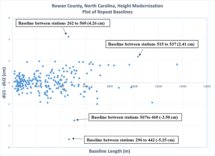
Figure 2 is a plot of the differences between repeat baselines. First, it should be noted that most baselines are less than 5 km and most repeat baselines differences are less than +/- 2 cm. There are some outliers, which is not unusual when performing GNSS surveys even when following all guidelines outlined in NGS 58. What is important is that these outliers are identified, and then additional observations are performed to meet the guidelines and obtain the desired accuracy of the survey.
The repeat baseline procedure helps to identify these outliers such as the baselines highlighted in figure 2. As noted in figure 2, the largest outliers are on two different baselines. These baselines should be re-observed to meet the NGS 58 guidelines. The requirement is to repeat the baseline on different days and at different time of the day. The reason for the requirement is to get two observations under different conditions and different satellite geometry. The user needs to determine which baseline is the outlier so he can ensure that he has two baselines with different satellite geometry. When a network is properly designed with short baselines and many loops, the results from a minimum-constraint least-squares adjustment can help identify the outlier.
Figure 2. Plot of repeat baselines for the NCGS Rowan County Height Modernization GNSS Project (does not include re-observations of repeat baselines that did not meet the 2 cm guideline).
Analyzing Loop Closures
Loop closures can be used to detect “bad” observations. If two loops with a common baseline have large closures, this may be an indication that the common baseline is an outlier. The following statement appeared in Part 2: “Please be aware that repeatability and loop closures do not always disclose all problems, and that is why it is important to adhere to the procedures outlined in NGS’ publications.” So why is it okay to use loop closures now?
Since users must repeat baselines on different days and at different times of the day, there are several different loops that can be generated from the individual baselines. If a repeat baseline difference is greater than 2 cm, then comparing the loop closures involved with the baseline may help determine which baseline is the outlier. As previously stated, according to NGS 58 guidelines, if a repeat baseline difference exceeds 2 cm, one of the baselines must be observed again, and baselines must be observed at least twice on two different days and at two different times of the day. If it can be determined which baseline is the potential outlier, the user will know which time of the day to re-observe the baseline. Therefore, loop closures can be very helpful in isolating errors when the user followed all of the guidelines outlined in the NGS 58 document.
Plotting Ellipsoid Height Residuals from Least Squares Adjustments
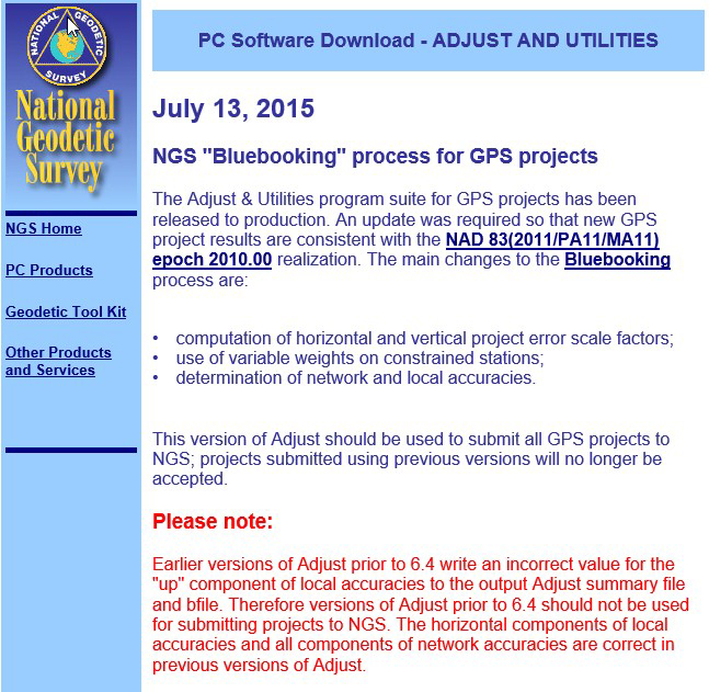
It is important that during the analysis of the GNSS-derived ellipsoid heights, the user performs a minimum-constraint least-squares adjustment and identifies potential outliers. This ensures that the GNSS-derived ellipsoid heights meet the user’s desired standards. This is not a complex procedure if the user knows how to perform a least-squares adjustment of GNSS data. Explaining least-squares adjustments is beyond the scope of this column. Today, most GNSS manufacturers provide support software that includes performing least-squares adjustments. NGS also provides software tools for validating data formats and performing adjustments. These tool can be found here. I used these tools to analyze and adjust the survey data of the Rowan County GNSS Height Modernization Project.
If users follow NGS guidelines and evaluate all repeat baselines, the adjustment results should confirm what has already been determined. For example, if a repeat baseline indicates a large difference between two vectors, then typically one of the residuals of one baseline should be larger than the other. Following NGS guidelines usually provides enough redundancy for the adjustment process to detect outliers and usually apply the residual to the appropriate observation, that is, the bad vector.
Like comparing repeat baselines, analyzing ellipsoid height residuals is also important. During this procedure, the user performs a 3D minimum-constraint least-squares adjustment of the GNSS survey project (constrain one latitude, one longitude and one ellipsoid height), plots the ellipsoid height residuals, and investigates all residuals greater than 2 cm.
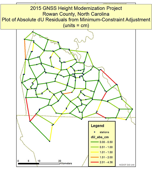
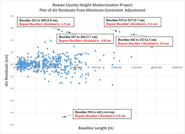
Figures 3 and 4 depict the dU residuals from a least-squares adjustment of the Rowan County Height Modernization Project. NGS’ adjustment program provides the vector residuals in dX, dY and dZ; and dN, dE and dU (local geodetic horizon coordinate system). dU residuals are not the same as dh residuals, but for all practical purposes can be analyzed just like dh residuals. Looking at Figures 3 and 4, a few items should be noted. First, all dU residuals are less than 2 cm except for five baselines. Four of the five baselines had repeat baselines that exceeded the 2 cm repeat baseline requirement (see Figure 2). For example, the plot of repeat baseline differences indicated that baseline between station 296 and 442 disagreed by 5.25 cm (see Figure 2). The plot of dU residuals (Figure 4) from the least-squares adjustment shows that one of the baseline’s residual is -4.4 cm and the other is 0.9 cm. The adjustment results are indicating which baseline needs to be re-observed to meet the guideline’s requirement of repeat baselines on two different days at two different times of the day. That’s all there is to it, when the user follows NGS guidelines exactly as prescribed.
Figure 3. Plot depicting absolute dU residuals from the NCGS GNSS Height Modernization Project (does not include re-observations of repeat baselines that did not meet the 2 cm guideline).Figure 4. Plot of all residuals from the NCGS Rowan County GNSS Height Modernization Project (does not include re-observations of repeat baselines that did not meet the 2 cm guideline).
The reader may have noticed that one large residual on the residual plot, baseline 442 to 253 (11.5 km), did not show up as a large different on the repeat baseline plot. There are several reasons why this could occur. For example, the stations involved in the baseline are not adjacent stations, so the baseline wasn’t repeated; the repeat baseline closure was large, but not greater than 2 cm; or the pair of stations are involved with many vectors and the one vector is inconsistent with the other vectors. Regardless of the reason, if there’s enough redundant observations to and from a station and the repeat baselines don’t indicate a problem, then the adjustment is doing what it’s designed to do; that is, detecting outliers and reducing their influence on the final adjusted height. In this particular case, the repeat baseline closure between stations 442 and 253 was 1.84 cm, which meets the NGS 58 guideline of 2 cm. The adjustment uses all of the data to determine the best set of coordinates. Based on the repeat baselines and loops surrounding the two stations, the adjustment indicated that one of the vectors fits better with the other vectors surrounding the two stations. Per the requirement of NGS 58 guidelines, the NCGS re-observed all five baselines with large residuals.
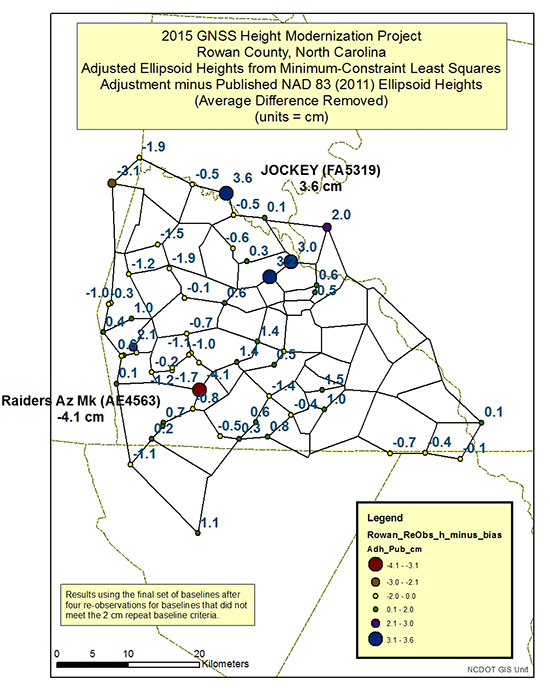
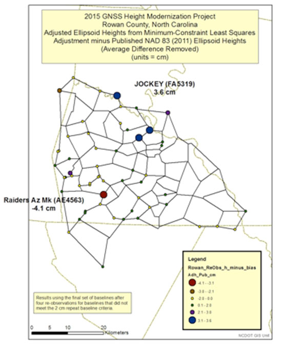
After all outliers are detected and removed from the adjustment, the user should compare the adjusted ellipsoid heights with the latest published ellipsoid heights, that is, NGS published NAD 83 (2011) ellipsoid heights. Figures 5 and 6 are plots of the adjusted ellipsoid heights from a minimum-constraint least-squares adjustment minus the NAD 83 (2011) ellipsoid heights. Since this was a minimum-constraint adjustment (that is, only one latitude, one longitude and one ellipsoid height value were constrained), a bias shift based on the average differences was removed from all differences. Most of the differences agree within +/- 2 cm. There are several that are greater than +/- 2 cm, but only one is greater than +/- 4 cm.
As mentioned in Part 2, many of the older GPS survey projects that were part of the NAD 83 (2011) network adjustment were not Height Modernization projects and were not performed following the NGS 58 guidelines. That is, most baselines are greater than 10 km and were not repeated. Therefore, in my opinion, many of the published ellipsoid heights local-height accuracies may be optimistic. The user should consider this when determining whether their results are more accurate than the published values. NGS’ Constrained Adjustment Guidelines for incorporating GNSS project data into NAD 83 (2011) state, “As a general rule, if the adjusted values of the constrained coordinates of a station shift by more than 2 cm horizontally and/or 4 cm in height, its horizontal coordinates and/or ellipsoid height, respectively, should be unconstrained.”
The stations that have height differences greater than 4 cm should be investigated. In addition, stations that have large relative height differences (greater than 4 cm) between closely spaced neighbors should also be investigated. For example, station Jockey’s difference is 3.6 cm, and two of its neighbors’ differences are only -0.5 cm. The relative difference exceeds 4 cm [3.6 cm – (-0.5 cm)] between two closely spaced stations.
Figure 5. Plot of adjusted ellipsoid height minus published NAD 83 (2011) Ellipsoid Heights (the number is the difference for that particular station; units = cm).Figure 6. Plot of adjusted ellipsoid height minus published NAD 83 (2011) published heights.
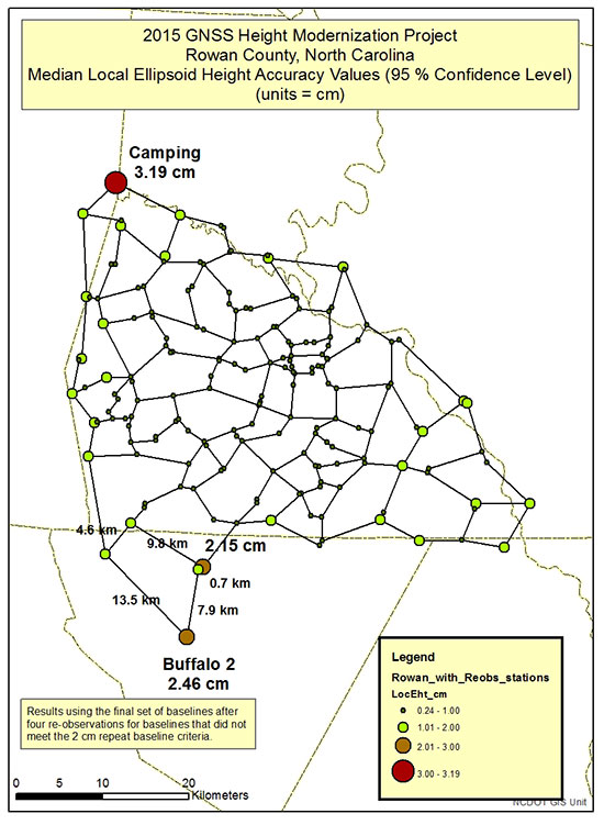
It is important to understand the quality of the adjusted ellipsoid heights. When analyzing the project’s ellipsoid heights, the user should compute the local ellipsoid height accuracy values. Part 2 discussed NAD 83 (2011) network and local accuracies. NGS’ adjustment program has an option of computing network and local accuracy values.
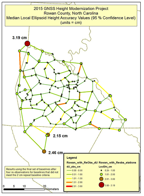
Figures 7 and 8 are plots of NCGS Rowan County GNSS Height Modernization median local ellipsoid height accuracy values. Stations that have local ellipsoid height accuracy values greater than 2 cm should be investigated. Figure 7 highlights the two largest median local ellipsoid height values [Camping (3.19 cm) and Buffalo 2 (2.46 cm)]. The observations and residuals of the baselines in the area should be closely analyzed.
Figure 8 is a plot of the local ellipsoid height accuracy value with the absolute dU residual values. If the user follows all of the NGS 58 guidelines, then all baseline residuals should be small (less than 2 cm). In this project, the largest “dU” residual is 1.86 cm. Saying that, the network design could be modified to try to improve a station’s median local ellipsoid height accuracy value.
For example, station Buffalo 2 has a median local ellipsoid height accuracy value of 2.46 cm (see Figure 7). It’s only involved in one loop, and it’s relatively large. The loop has five baselines consisting of lengths of 13.5 km, 9.8 km, 7.9 km, 4.6 km and 0.7 km. Two of the baselines lengths are greater than the guideline’s average baseline recommendation of 7 km, but all repeat baselines meet the 2 cm guidelines, and all residuals are “reasonable.” Adding another baseline between two different stations to create two smaller loops from the one larger loop would decrease the size of the loop and increase the redundancy in the network.
In this particular case, station Buffalo 2 has a published NAD 83 (2011) ellipsoid height, and the difference between the adjusted height and the published height is only 1.1 cm (Figure 5), indicating the new survey is consistent with the old survey. Station Camping also has a published NAD 83 (2011) ellipsoid height, and the difference between the adjusted ellipsoid height and published height is -1.9 cm (Figure 5). Once again, this indicates that the Rowan County GNSS survey is consistent with the previous survey.
This column focused on describing procedures for analyzing a project’s GNSS-derived ellipsoid heights. As previously stated, it important to ensure that your GNSS-derived ellipsoid heights meet the desired accuracy of the project before using the survey data to estimate GNSS-derived orthometric heights.
Figure 7. Plot of NCGS Rowan County Height Modernization project’s median local ellipsoid height accuracy values.Figure 8. Plot of NCGS Rowan County Height Modernization project’s median local ellipsoid height accuracy values and absolute dU residuals.
So far, this series has addressed the following topics:
basic concepts of GNSS-derived heights
NGS’ guidelines for establishing GNSS-derived ellipsoid heights (NGS 58)
differences between hybrid and scientific geoid models, and
procedures and tools for detecting GNSS-derived ellipsoid height data outliers.
These four columns were meant to provide the reader with basic concepts and procedures for estimating GNSS-derived ellipsoid heights.
My next column, which will appear in the February 2016 Survey Scene newsletter, will discuss procedures for estimating GNSS-derived orthometric heights. Determining valid NAVD 88 published heights is very important when using GNSS data and geoid models to estimate GNSS-derived orthometric heights. NGS has documented these procedures in NOAA Technical Memorandum NOS NGS-59. The NGS 59 guidelines are separated into three basic rules, four control requirements and five procedures that need to be adhered to for computing accurate NAVD 88 GNSS-derived orthometric heights. The next column will address the NGS 59 guidelines.