Editor Don Jewell Talks with the Air Force General Heading Space Command: His Views, Use, and Plans for GPS
Defense editor Don Jewell is a retired Air Force officer who served for 30 years; many of his former peers and contemporaries are currently senior officers in today’s U.S. Air Force. Don sat down recently with General C. Robert Kehler, Commander of the U.S. Air Force Space Command, whom he has known and worked with for more than 20 years, to discuss GPS from the four-star point of view.
Don Jewell (DJ): General Kehler, thanks for taking the time to have this discussion today. I would like to keep this very informal, more of a conversation, like the days when you and I and Willie Shelton [now Lt. Gen. Shelton, USAF] sat around on your lanai, sharing a brew, telling war stories, and solving the world’s problems.
General Kehler (GK): Believe me, Don, there are days when I wish we were still doing that. I appreciate the opportunity to have a conversation with you.
DJ: Great. Sir, to get to the crux of the matter, as the senior warfighter for space, how do you see GPS in the future, and how does it contribute to the joint fight?
GK: Don, you know this, as may many of your readers at GPS World, but I don’t believe we can say it often enough: GPS is the primary source of position, navigation, and timing (PNT) information for the Department of Defense, and it will remain that way at least until the year 2030. This has been a remarkably successful program, supporting the joint warfighter in nearly every aspect of joint operations. How GPS supports joint operations, whether it’s the individual soldier, sailor, airman, Marine, or Coast Guardsman, who is on the ground or inflight or who happens to be in the dark in a mountainous region somewhere or in the flat expanse of the desert — it doesn’t much matter. GPS has been their constant companion now for many years. They have come to rely on GPS in ways that help them do their job better, and it allows them to perform missions that in the past they would not have been able to perform in this kind of a manner, with this kind of perfectness.
GPS is going to remain the foundation of the PNT strategy. And with the modernization effort that we have underway in GPS, we are going to make sure that it remains the world’s premier source of position, navigation, and timing information, and in particular that it remains woven through the fabric of the joint warfighting network.
DJ: This portends an excellent future for GPS, despite comments by the Air Force Chief of Staff and Gen. “Hoss” Cartwright, vice chairman of the Joint Chiefs of Staff, that we should move away from GPS. Do the Chief’s comments cause you any concern?
GK: They do not cause me any concern. We are committed to keeping GPS the gold standard. We have a commitment in that regard. I understand exactly what the Chief of Staff said and why. I will be happy to discuss that more.
DJ: We’ll table that for now, and get to it later if we have the time. I have often heard you say in your GPS update and status briefings that GPS is one of your good systems. Indeed, you have described it as one of the systems you don’t have to worry about too much, because it works. It would be interesting to ascertain how you know when you are doing a good job with GPS. How do you know it works? For example, do you receive comments, e-mails, or letters from warfighters?
GK: I think there are really two big ways that we know we are doing a good job with GPS. First of all, we measure our performance against the standard. What the users see, of course, is accuracy and satellite availability. Those have become our two primary standards. We make sure we are performing up to those standards. And in fact, as you know, we continually outperform those documented standards and the requirements that we have.
We also look, not only at the satellites, but at the ground command and control (C2) system and the ground support network. We make sure those elements are always up and running as well. From a numbers standpoint, from a “how well are we meeting the standards we have set for ourselves” standpoint, we exceed those standards. We exceed in terms of accuracy and availability, both the satellite system and the ground-supporting infrastructure as well.
But these days, I will tell you, I think the numbers are interesting, but what I think we look at just as hard is how the public talks about GPS.
And if you look today, GPS, at least in my opinion, is everywhere in the public conscience. I was saying earlier today, you really don’t have to go much farther than your television set. Almost any evening you turn the TV on you’ll hear something about GPS. You’ll either hear people who are equating their product to GPS, or you’ll hear in a television show someone mention GPS or their GPS device. And that is without it being a program about the satellites themselves, or the U.S. Air Force, or the things we do at Schriever Air Force Base to make it all work.
My view is that the fact that we get this informal public feedback constantly, and that it’s positive, says a lot about how good a job we are doing as well. When your program becomes a new word in the English language, I think that says something about success. Any more, if you say GPS to people they might not point to a satellite, they might point to the little device they are holding in their hand, but they understand somebody is providing that for them and that it is working well.
The final piece to that is also our civil partners. You know we have a GPS Executive Committee (PNT ExCom) inside the government that meets periodically to have conversations about the way ahead on GPS for the entire government, and by extension for the United States. The feedback that we get at those meetings, and unfortunately I can’t get to every one of them, but in those that I have attended, the feedback has been universally positive.
We just had a Civil Focus Day recently, and the feedback we got was universally positive. Are there things we can do better? Yes, of course there are, there are always things you can do better, but I can tell that we are doing a good job with GPS, not only because of the numbers that we look at but because of the feedback that we get, and the way GPS has been accepted and adopted, if you will, as part of the lexicon.
DJ: You’re absolutely right about the positive feedback. I attended Civil Focus Day, wearing a different hat, as you know, and I agree, everybody was onboard and positive about GPS.
The next topic revolves around how your scorecard is graded by the joint community, and do you have a way of actually getting feedback from the warfighter?
GK: Yes, as I said, we are graded or we grade ourselves primarily on accuracy and availability as they are documented for us in the performance standards. In watching those numbers, we know that we are exceeding the performance standards that we set for ourselves. But we also receive feedback directly from the warfighters. We receive feedback from the military users through the GPS Operations Center (GPSOC). You know, and I think most of your readers know, that there is a way that you can directly contact what we call the GPSOC 24 hours a day, seven days a week, and we find that both our military and civilian users do that.
Another way that we receive feedback is through the Coa
st Guard Navigation Center (NAVCEN), where they are specifically watching and helping us watch the performance of GPS. We get feedback directly from them as well. But much like the prior topic, there are also other ways that we get feedback.
For example, in each of our theaters of operations, for each of our combatant commanders, the joint or combined force air component commander is also designated as the space coordinating authority. And working for that space coordinating authority in the AOC (Air Operations Center) is someone called the director of space forces, an Air Force officer who is responsible for making sure that the space support is there when it needs to be and in the fashion that it needs to be. Those directors of space forces also have a small staff working with the combined force air component commanders.
They are getting direct feedback from the warfighters as well. They are either getting it as a normal course of business, on a day-in day-out basis, or they are asking for it specifically as well. We are also getting direct feedback from the units themselves. We have made contact through a number of our forward space people. We work with Army Space and Missile Defense Command and as a matter of fact we have talked with the Marines and others directly. We don’t wait for their feedback, we go out and solicit it also, and we actually help them solve some very difficult problems that we had early on in the conflict with some of our weapons systems that we have now fixed.
We are mindful, we know when certain operations are underway, we deconflict that with activities in the [GPS] constellation, making sure that we are providing the very best service all the time. We are embedded through the planning process in the theaters with military operations and with space professionals who are in the planning cells and Air Operations Centers. We are very comfortable. We are getting constant feedback from the warfighters in addition to the scoring we do ourselves and against the performance standards.
DJ: As you know, in many of my articles I frequently comment that where GPS is concerned, geometry and numbers matter. In that regard you recently approved a 24+3 GPS constellation change. Now we get a good many letters from warfighters at GPS World, and some letters are all about GPS accuracy as you spoke of earlier, but actually more letters mention GPS availability as being critical. Where do you stand on the debate of what is more critical, accuracy or availability, as far as the warfighters are concerned?
GK: We don’t separate the two children here, availability and accuracy. Obviously, it doesn’t mean a lot to us if you have high availability and not high accuracy, or if you have high accuracy and not high availability. They go together, and we work both of those issues. We try to make sure that we have the highest availability and accuracy. The accuracy numbers have been very good, as you know. We have been trying to improve availability, particularly for users in impeded environments. We are doing that by taking advantage of the largest constellation of operational GPS satellites we have ever had on orbit. We have begun to adjust the way we have configured the on-orbit constellation.
You called it 24+3, and we were all calling it 24+3 for a while. Now we are calling it Expandable 24, because those are the words that are actually in the Standard Positioning Service Performance Standard. We are expanding the available operational useful slots from 24 in the constellation to 27, and that movement is underway. This should result in improved availability for users in challenged areas like mountainous terrain, deep canyons, and in some cases urban terrain. It improves those kinds of availability numbers worldwide for everyone, for all users. This is not just for warfighters, it’s for all users.
We have begun the movement of the satellites (SVs), and because we are trying to balance on-orbit longevity with movement, it will take us a period of months to move the satellites to the new locations. That movement is underway, and the availability numbers should begin to improve as the movement begins; you don’t have to wait until they are all in their final locations.
By the way, as an aside, just last night, I was driving in Washington [D.C.] and I was using the navigation feature in my cell phone. One of the things it tells you is how many satellites are in view as you are driving along. Now, just to be clear, I was not driving, I was a passenger in the car, so I was not distracted by trying to drive. But I sat there with the thing in my lap, watching it while we were driving through the streets of Washington, D.C., and there were never less than nine satellites in view. At best I noticed that there were 12.
So I thought about that for a minute. Half of the constellation was occasionally in view as we were driving around the streets of Washington. This is pretty powerful, and we are talking about availability. I sat there thinking to myself, yo, if we can help somebody out there — turn that availability when they need it into the right number of satellites — this is a pretty powerful movement that we’ve got going.
DJ: It is, and what you just said about being in the back of the car reminds me about what General Chuck Horner (USAF, ret.) said after he retired as commander in chief, Space Command. He said you know you are truly retired as a four-star general when you go out and get in the back of the car in the morning, and nothing happens.
GK: You’re exactly right. I have a new officer aide who had never been stationed in Washington, and can’t survive in Washington without some kind of a GPS navigation device. He had one going in the front seat, and I had mine going in the backseat, and we were comparing notes as we drove along. It really is pretty remarkable.
DJ: Our readers will he happy to hear that you also have dueling GPSs. I have readers write and say they have up to three or four going at one time on long trips, comparing different GPS device accuracies and interfaces.
GPS has truly been a life-changing event for many of our users, especially the warfighters. I receive hundreds of letters and e-mails from warfighters and this move to Expandable 24 is meeting with unanimous approval.
GK: That’s good to know, and I must say that originated here. Actually, that originated with the IRT [GPS Independent Review Team], as you well know. We then took that to Strategic Command, and Strategic Command embraced it. General Chilton embraced it immediately, and I think that we have done the right thing here. The downside risk here did not outweigh the positive impact that we think we can have on people who need expanded availability.
DJ: Sir, as I said before, wearing a different hat, I attended your Civil Focus Day and I thought it was outstanding. Do you have any comments you would like to make concerning that event, and do you think you achieved your goals?
GK: We did achieve our goals, because our primary goal is improving communication and cooperation, as well as making sure we’ve got a stronger working relationship between the civil and military GPS communities. In that regard I think our goal was achieved. We addressed a lot of crucial concerns that impact both communities. We emphasized that the ongoing GPS modernization and enhancement efforts are going to be transparent to the civil users, and in fact will result in pretty dramatic improvements for civil users:more signals and other enhancements that I think are going to be useful as time goes by. In that regard I was very pleased.
We had a number of very senior people throughout the government who expressed their interest in GPS with their attendance. We had seen, as you know, additional commitment from some of the other [U.S.] government agencies to be supportive in helping to invest in GPS, which I think is very positive. I just think that in general terms we want to make ourselves more transparent in terms of how we are dealing with the constellation and the future of the constellation.
We recognize in Air Force Space Command the unique role that we have for this global utility that the United States of America provides free of charge for everyone else on planet Earth. We recognize that with the use of this and the increasing impact it has on all our lives, comes a unique responsibility for stewardship. We have embraced that responsibility, and that means we have to be transparent and we have to have a collaborative team that we work with, and that was a large part of the Civil Focus Day.
DJ: Many of the proposed systems that may or will one day compete with or complement the GPS are on hold, delayed, or still not at full operational capability. What is your viewpoint on where we stand in relationship to these systems, such as GLONASS, Galileo, and Beidou, for example?
GK: Our objective from an Air Force standpoint has been to support the U.S. government’s goal of wanting to engage in cooperative activities related to space-based PNT, and I think the focus of that cooperation has been to try and ensure that we have compatibility between GPS and other space-based PNT systems. There is a goal on our part to make sure we can be compatible and interoperable. There is a goal on our part to make sure we are protecting our national security interests and that we are maintaining a level playing field in the global market for space-based PNT goods and services.
Those are our objectives, those are the national objectives of the U.S., and the Air Force is supporting those objectives through our management and operation of the GPS constellation. That will continue to be our posture: to make sure, as best we can, to have fostered successful relationships on space-based PNT.
DJ: You certainly can’t ask for more than that. The objectives are laudable, but on the surface they don’t necessarily fit well with the recent comments by the chief of staff of the USAF, and I guess that brings us to the topic we briefly discussed earlier. Do you fully understand where the chief was going with his comments concerning GPS at Tufts University last month, and do you have any comments that might help our readers put the chief’s remarks in the proper perspective?
GK: I do. I was present when General Schwartz made his comments, and honestly I understood what he was saying and why. I think that he was misunderstood in implication. I think what he said was misapplied by some. In my view, General Schwartz fully supports GPS. What he was doing, though, is he was talking about GPS and its value for military operations.
What we know is that, like any other military capability that we rely on for important pieces of our warfighting force, GPS will be challenged by a determined enemy that is interested in trying to defeat U.S. forces on the field of battle somewhere. He was reminding us that we need to be mindful of that:adversaries could potentially exploit GPS as a vulnerability because of the way we have come to rely on our GPS for our own American way of warfare. And because it is such a critical system to the warfighter, it will be an attractive target to any would-be enemy.
Having said that, his point was, with which I fully agree, we have to be diligent in finding ways to operate with the same accuracy and precision in the event that GPS is degraded. That’s exactly what the GPS Modernization Program is designed to do. But this goes beyond GPS as well, it goes into other things, for example, missiles are guided to targets or munitions are guided to targets in some cases by GPS, in some cases by inertial systems, and in some cases by a combination of both. It would be foolish for us to not have provided for the eventuality where GPS will be jammed. But again he was talking about a military environment here; he was not talking about the global environment, he was talking about the military environment.
I recommend to people sometimes that they should go look at, well, pick your search engine of choice on your home computer, and type in “GPS jammers” and see what you get. There is a proliferation of GPS jammers around the world, everything from the sizes that will plug into the cigarette lighter in your car to large devices that are sold internationally for military purposes. We know that GPS will be contested when or if we are involved in any military conflict. The chief was warning us that we need to take that into account, and I believe he was exactly right to do it.
DJ: Thank you, sir, that helps clarify the Chief’s remarks considerably. I just wish he had said what you said versus what he said. Sometimes senior leaders are just too close to the problem and they erroneously assume their audience has information, knowledge, or insights that they in fact just do not possess, and it skews their perception of the senior leader’s remarks.
The last topic I would like to discuss concerns the infamous AEP 5.5C update that did not go quite as well as planned. Again in this instance, the public perception may be skewed by a lack of information and a lack of communication. I know you are fully up to speed on this issue; what are your thoughts?
GK: I would make a couple of points about upgrading the ground software. First, with this latest version of the ground software, AEP 5.5 and all of its iterations, we learned a lot about the complexity of the GPS system, how complex it has become. We learned a lot about standards, and what happens if you make receivers and you don’t follow the standards, because there was nothing wrong with the [AEP] 5.5 software in this case. The issue was in the receivers — a very small percentage of our military receivers — where the manufacturers did not comply with the standards. We hold ourselves to a set of standards, we publish those standards, as you well know, and it is important for people who are making GPS devices to follow those standards.
Now here’s what we learned, though. We learned that not only is it important to follow the standards, but we learned that we can do better in how extensively we test prior to installing software. By that I mean — not that we didn’t test extensively before — increase the population of receivers that we test against and the rigor with which we test them, would be a better way to say this.
The other thing we learned is that collaboration and cooperation needs to be more robust, such that we are doing these upgrades on an active basis, not a passive basis. What we had been doing before is we would publish a NANU and say that we were about to do an upgrade to the ground software. We would then do the upgrade. We would wait to find out what was happening. What we learned this time was, that is probably too passive as we go to the future. Not only will we test more extensively across a broader range of GPS devices, but we will also put [receivers] in place, in a series of predetermined locations, if you will, where we will contact them actively to find out as we are progressing whether they are encountering any difficulties. We did learn a lot here.
We also learned that these upgrades need to be done in a fashion that is repeatable, so that every time we do this we will have a process in place that allows us to treat them roughly the same, depending on the magnitude and risk associated with the change, if you will, in terms of how we intend to go forward. I think we learned a lot about vetting and we learned a lot about execution. We
reminded ourselves again why standards are so important, and we reminded ourselves why partnerships are so important and why rapid feedback is important: so that we can deal with problems as they emerge.
We also learned something for the longer term, Don. We learned that we probably need better simulation tools as we look to the future, because you know there is only one active system, and it is the active system. It has become so complicated that there are hundreds of millions of receivers out there, as you well know, and the likelihood that we can characterize all of them in advance of a software drop is pretty low. We are going to have to get better at following a simulation as we go forward.
The most significant piece of data, though, from all this was there was nothing wrong with AEP 5.5. It performed exactly the way it was designed. The issues that were encountered were anomalies in user equipment, and that user equipment was identified because it did not follow the standards.
DJ: General Kehler, do you have any closing remarks for our readers, a message you want to make sure gets heard?
GK: Don, we understand the unique position that we are in as stewards of GPS. This is unusual, I believe, throughout the U.S. military, that a military service would have this type of responsibility for a system that has this kind of global impact. And it has that global impact 24 hours a day, seven days a week, 365 days a year. We recognize that unique responsibility that we have.
We know that means we have to be transparent about the way we conduct our business. We think that we are doing much better at that, and we will get better at that even more as we look to the future.
Our bottom line is that we believe that GPS is the gold standard today for the world. We intend to keep it that way as we look to the future, and we will allow the performance of the GPS system to speak for itself. We are very, very proud of the job that we do regarding GPS.
The young — many very young — men and women who operate and fly that constellation everyday, the outstanding technical people we have who design and build the satellites, the phenomenal launch team that we have that gets them to the Cape and gets them successfully on orbit — all of these pieces that are taken together along with, by the way, a civil group of participants from across the government who work very hard at all of this, along with independent folks who are on our review teams and elsewhere as well as the industry, the broader industry —this is a remarkable success story that has now influenced virtually everything we do, everywhere on the face of the planet. I think we ought to be very proud of that, and I can tell you that this Command is extraordinarily proud of it and recognizes that this puts a unique burden on us to deliver. We are going to continue to do just that.
DJ: That’s a great message and a very important one. In closing, might I ask you about your future? Rumor has it that there are plans afoot for you to move onward and upward.
GK: Don, my wife keeps saying that we go to Myrna — she is the dry cleaner and tailor down the street here — to find out where we are going.
I don’t know. I have been here two and a half years, Don, and typically this assignment will last about three years. That will take us into late summer, early fall, and I honestly, honestly do not know what happens with us next. We are going to have to wait and see what the pleasure is of my superiors and how all the pieces sort of fit together.
I think you know, when you get to be a four-star, there are a lot of factors that come to bear. At this point we will just have to wait and see. The only thing that I am worried about right now is the job that I’ve got, and I will be very, very pleased to stay here. We could stay here for 10 more years, and I would be delighted to stay here because this is a magnificent command.
We are doing phenomenally important work, and I am very proud of the people in Air Force Space Command. This is a wonderful, wonderful group of people.
DJ: You should be proud of them, sir. We get a lot of mail about what a great job the Air Force is doing as the steward of GPS. Our mail is always very positive concerning Air Force Space Command. I want you to know, sir, in closing, that working with Colonel Ford and Colonel Buckman has been a real pleasure. Your folks have been just super.
GK: I think so, too, and I don’t tell them that enough, really. We’ve got a great team here at headquarters, and we’ve got a great team across this command. We are delighted to have cyber responsibilities now, and there is clearly a relationship between space and cyberspace, and we see it. Every time I get a chance to commend the people in the Command, I like to take the opportunity to do so.
DJ: Thank you for your time today, sir. I know how busy you are, and I think we should find the time soon to sit down and have another discussion, possibly on cyberspace.
GK: That’s fine with me. Thanks, Don.
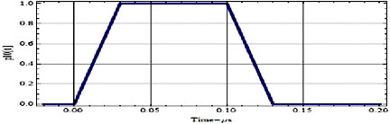
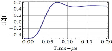
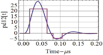
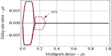
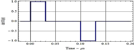 FIGURE 2. Trapezoidal PN (1 Mcps) waveform pulse and its time derivative with a 0.1-microsecond rise time.
![FIGURE 3. Discriminator channel, d[e], and (bottom) discriminator output, R[e] Rd[e], for the 1.0 Mcps PN with the optimum 0.1-microsecond reference and the 0.1-microsecond rise-time trapezoidal waveform.](https://stage.globalpositioningnews.com/wp-content/uploads/2010/05/EA-3.jpg)