Blog

  • Innovation: GPS, GLONASS and More

    Innovation: GPS, GLONASS and More

    Multiple Constellation Processing in the International GNSS Service

    By Tim Springer and Rolf Dach

    Does combining GPS and GLONASS observations make a difference? The International GNSS Service (IGS) has been providing such data for several years. Representatives from two IGS analysis centers discuss the past, present, and future of IGS GNSS monitoring and product development.

    INNOVATION INSIGHTS by Richard Langley
    INNOVATION INSIGHTS by Richard Langley

    ARE WE THERE YET — at a multiple-constellation GNSS world? The European Galileo system only has two test satellites in orbit, with constellation completion not scheduled until 2014. The Chinese Beidou/Compass system has launched some test satellites, but global coverage is not promised until 2020. And the first Japanese Quasi-Zenith Satellite System space vehicle is scheduled for launch this year with the system not fully operational until 2013. So, does this mean GPS is still the only game in town? No, not by a long shot. We have overlooked Russia’s GLONASS.

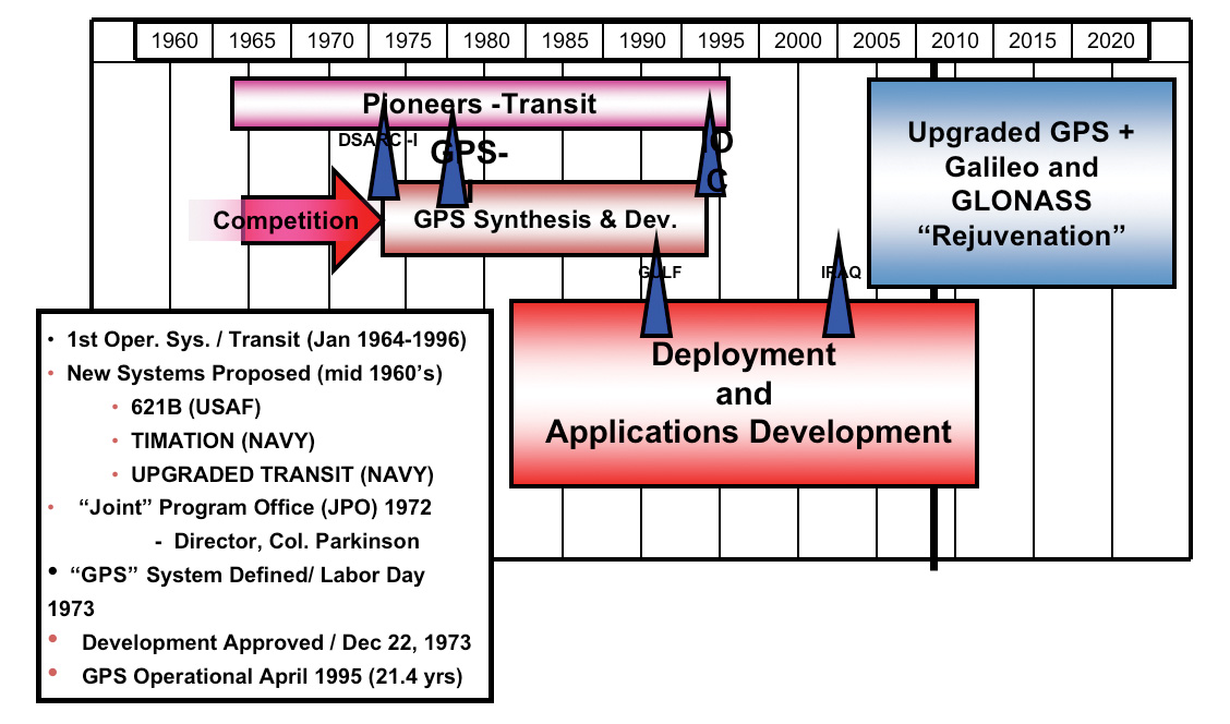
    Standing for Global’naya Navigatsionnaya Sputnikova Sistema, GLONASS was conceived by the former Soviet Ministry of Defence in the 1970s, perhaps as a response to the announced development of GPS. The first satellite was launched on October 12, 1982. But because of launch failures and the characteristically brief lives of the satellites, a further 70 satellites were launched before a fully populated constellation of 24 functioning satellites was achieved in early 1996. Unfortunately, the full constellation was short-lived. Russia’s economic difficulties following the dismantling of the Soviet Union hurt GLONASS. Funds were not available, and by 2002 the constellation had dropped to as few as seven satellites, with only six available during maintenance operations! But Russia’s fortunes turned around, and with support from the Russian hierarchy, GLONASS was reborn. Longer-lived satellites were launched, as many as six per year, and slowly but surely the constellation has grown to 21, with two in-orbit spares.

    But are there any users outside Russia? Although dual-system GPS/GLONASS receivers have been around for at least a decade, manufacturers have taken notice of GLONASS’s recent phoenix-like rebirth. All of the high-end manufacturers now offer receivers with GLONASS capability. Does combining GPS and GLONASS observations make a difference? You bet — just ask any surveyor who uses both systems in the real-time kinematic (RTK) approach. Scientific applications requiring high-accuracy satellite orbit and clock data also benefit. The International GNSS Service (IGS) has been providing such data for several years, and in this month’s article representatives from two IGS analysis centers discuss the past, present, and future of IGS GNSS monitoring and product development.

    So, getting back to our question, are we there yet? Many early adopters of GPS plus GLONASS data and products would reply with a resounding “yes.”


    “Innovation” features discussions about advances in GPS technology, its applications, and the fundamentals of GPS positioning. The column is coordinated by Richard Langley, Department of Geodesy and Geomatics Engineering, University of New Brunswick.


    In 2005, the International GPS Service (IGS) was renamed the International GNSS Service. With this change, the IGS governing board and the IGS community expressed their expectation to extend activities from the well-established GPS to other active and planned global navigation satellite systems such as GLONASS, Galileo, and Compass. Meanwhile, the GLONASS satellite constellation, as well as the IGS GNSS tracking network, have evolved significantly. Since 2003, the GLONASS satellite constellation has been improving steadily, leading to the current, May 2010, constellation with 21 operational satellites and two in-orbit spares. And starting in 2008, the GNSS capabilities of the IGS tracking network have been greatly enhanced giving rise to a truly global GNSS tracking system with more than 100 GNSS (GPS plus GLONASS) receivers. The almost-complete GLONASS satellite constellation, coupled with a readily available global tracking network with high-quality receivers, have greatly increased the interest in and need for GNSS products such as precise satellite orbit ephemerides. However, the IGS analysis center products are still mainly GPS-only. Only two analysis centers provide true multi-GNSS solutions. Two analysis centers provide GLONASS-only solutions (a GLONASS combined IGS product is available but without accurate clocks). No combined IGS GNSS product exists. In view of the large interest from the user community, this is a really disappointing situation. In particular, because experiences gathered with handling GPS plus GLONASS will make the incorporation of other GNSS such as Galileo, Compass, and the Quasi-Zenith Satellite System (QZSS) that much easier.

    However, during a meeting of the IGS analysis centers in December 2009, it became clear that many of the centers had started to implement and enhance the GLONASS processing capabilities in their software. This was happening as a direct consequence of the improvements in the GLONASS constellation, the IGS GNSS tracking network, and increased user interest (if not demand). Throughout 2010 and 2011, we will therefore see a significant increase in the number of true GNSS solutions within the IGS. A very positive development for the GNSS world.

    In this article, we give an overview of the recent developments in the area of multi-GNSS processing within the IGS in general, but with a focus on the activities of the two analysis centers in the IGS that are leading the GNSS efforts: the Center for Orbit Determination in Europe (CODE) and the European Space Operations Center (ESOC) of the European Space Agency.

    Why GNSS?

    Within the IGS, we are often confronted with the question: Why GNSS? Why should I go through the burden of adding GNSS capabilities to my software, having larger processing loads, and so on, for little or no benefit? Well, from an IGS analysis center point of view, this question is valid. The accuracies achieved with GPS alone are so good that there will be little visible benefit of including another system. Nevertheless, there are indeed benefits.

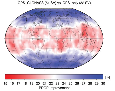
    There is a large number of users worldwide who would see benefits of using GNSS products compared to GPS-only products. Clearly, all real-time users will benefit enormously from the increased number of satellites. Figure 1, showing the so-called position dilution of precision (PDOP), demonstrates this very clearly. The two panels in Figure 1 show the GPS-only PDOP and the GPS-plus-GLONASS PDOP using the satellite constellation of May 3, 2009.

    FIGURE 1A. Effect of GLONASS on position dilution of precision.
    FIGURE 1A. Effect of GLONASS on position dilution of precision.
    FIGURE 1B. Effect of GLONASS on position dilution of precision.
    FIGURE 1B. Effect of GLONASS on position dilution of precision.

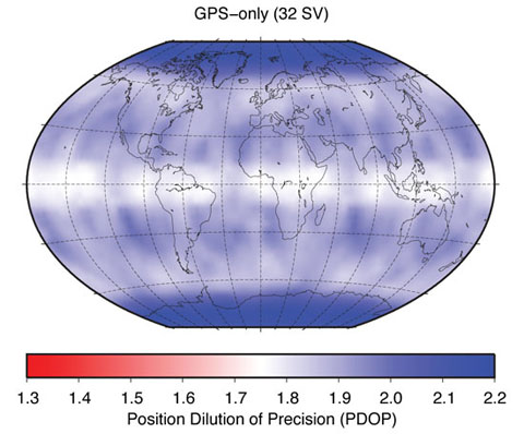
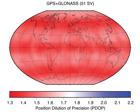
    Figure 2 shows the PDOP improvement in percentage when comparing the GPS-only to the GPS-plus-GLONASS PDOP values. At high latitudes, that is, above 55 degrees, the improvement is at the 30 percent level. At mid-latitudes, the improvements are still well above 15 percent, demonstrating the significant improvements real-time GNSS users may expect compared to real-time GPS-only users.

    Figure 2. Position dilution of precision improvement using GLONASS.
    Figure 2. Position dilution of precision improvement using GLONASS.

    With the current GPS constellation, daily solutions are not limited by the number of available satellites, but rather by the analysis models (such as that for the troposphere), calibration uncertainties (such as models for antenna phase-center variation), and environmental effects (such as multipath). For these reasons, IGS-like processing strategies, in which data from reference stations are processed in 24-hour batches, will not show clear benefits from adding data from more satellites and other systems.

    However, besides real-time users, users at high latitudes (including the whole of Canada and most of Europe) will see improvements. Recently, several researchers have noticed that for latitudes higher than 50 degrees, the addition of GLONASS brings benefit. This is, of course, thanks to the higher orbital inclination of the GLONASS satellites (about 64 degrees) compared to the inclination of the GPS satellites (about 55 degrees), which is also very nicely demonstrated in the PDOP (see Figure 1). So, from a service point of view — the “S” in IGS — there is a clear need to provide GNSS solutions to the user community. Besides offering significant benefits in terms of accuracy, the increased number of satellites will also make solutions more reliable and robust. The completely different repeat cycle of the GLONASS satellite orbits is especially important as it changes the sensitivity to multipath completely. Multipath effects in GPS-only data repeat almost perfectly from day to day with a 4-minute time shift giving rise to spurious, near yearly signals in GPS time series. Satellites from other constellations, such as GLONASS, introduce other system-related frequencies, which results in a general reduction of such GNSS-induced frequencies in a multi-GNSS solution.

    Because of the constellation design, each GPS satellite follows its own ground track in each orbit cycle. That means that at a ground station, each GPS satellite is observed on one and the same track each day so that a systematic influence of a satellite (such as a mismodeling of the satellite antenna position with respect to the satellite’s center of mass) has a systematic effect on the obtained (daily) station positions. This systematic translation of satellite-related errors into station-related parameters doesn’t happen for any other GNSS constellation.

    IGS GNSS Analysis Centers

    A detailed description of the IGS is beyond the scope of this article; an excellent overview was provided in an earlier Innovation column. We simply point out here that it is important to know that the IGS serves as the reference in many GNSS applications by providing data and products of the highest possible quality. Very well known and widely used are the tracking data from the IGS station network — the raw pseudorange and carrier-phase measurements — and the orbit and clock products of the GPS satellites. The IGS generates these products by combining the orbit and clock solutions of the individual analysis centers that contribute to the IGS. For the GPS-only products, 10 different analysis centers contribute to three different product series called the ultra-rapid, rapid, and final products. The final products deliver the highest possible quality but have the longest delay, as they become available 12 days after the end of the observation week. The rapid products are roughly comparable in quality to the IGS final products, but they are delivered daily with a delay of only 17 hours after the end of the observation day. The ultra-rapid products are delivered four times per day 3 hours after the end of the last used observation. For example, at 03:00 UTC, an ultra-rapid product is delivered that used data up to 00:00 UTC. It consists of two parts: an estimated part and a predicted part that may be used for real-time purposes. The quality of the estimated part is very similar to that of the rapid products. The predicted part is, of course, significantly less accurate, although the orbits have an astonishing precision of well below 30 millimeters — much better than that of the orbits in the satellites’ broadcast navigation messages.

    In addition to these GPS-only products, there is also a GLONASS product. However, contrary to the GPS side of things, for GLONASS, only a final product is generated. Four analysis centers provide products for the IGS GLONASS combination: the Bundesamt für Kartographie und Geodäsie (BKG), Frankfurt am Main, Germany; CODE, based at the Astronomical Institute of the University of Bern, Switzerland; ESOC, Darmstadt, Germany; and the Information-Analytical Center (IAC) of Roscosmos, Moscow, Russia.

    The analysis centers BKG and IAC determine the GLONASS satellite orbits, introducing the information for the GPS satellites from the IGS solution without further estimation. The analysis center CODE provides, since May 2003, orbits for GPS and GLONASS based on a rigorously combined analysis of the data of both GNSS, that is, a true multi-GNSS solution. Since January 2008, ESOC follows this strategy as well. From these four analysis centers, only two, ESOC and IAC, provide satellite clock estimates for the GLONASS satellites. This situation prevents the IGS from making a robust and reliable combined GLONASS clock product. With four analysis centers contributing to the orbits, the IGS can and does make an excellent GLONASS combined orbit product.

    In our definition of true multi-GNSS solutions, the measurements from each system contribute to all relevant parameters to the same extent. This can only be achieved by the rigorous combined processing of the data from all available GNSS. The two-step approach, introducing the GPS solution when solving for the GLONASS orbits and satellite clocks, is regarded as an extension of a GPS-only solution to GLONASS. As the contributions from BKG and IAC in the IGS GLONASS product demonstrate, this two-step procedure provides excellent results.

    From a user point of view, a big disadvantage is the fact that the IGS does not provide a real GNSS product. The IGS provides a high-quality GPS product and a high-quality GLONASS orbit product, but there is no combined GNSS product. Also, the IGS is only capable of generating final GLONASS products because only two analysis centers, CODE and ESOC, submit GNSS products for the rapid and ultra–rapid products. IGS policy requires contributions from at least three analysis centers for a meaningful and robust combined product.

    Users of GNSS orbits and/or clocks therefore have to use the products of one of the individual analysis centers or combine the GPS-only and GLONASS-only products from the IGS. Here, the GNSS products of the CODE and ESOC analysis centers are clearly preferable over those of the IGS and other analysis centers since these are the only two true GNSS products that guarantee the full consistency between the two GNSS.

    GLONASS Tracking Network

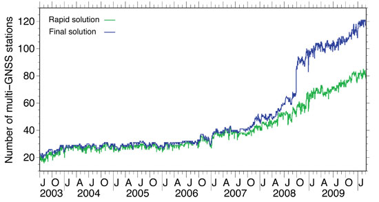
    Until 2003, the IGS had established a GLONASS tracking network of merely 20 stations. In 2003, this number grew rapidly from 20 to 30, but after 2003 the number of stations remained stable for quite a long time with a very inhomogeneous distribution. For example, there were only a few stations in the whole western hemisphere. In 2006/2007, a new generation of combined GPS/GLONASS receivers became available, produced by several well–known GPS receiver manufacturers. With this new equipment available, the number of GLONASS tracking stations in the IGS network started to increase steadily. In 2008, the increase rate went up significantly (see Figure 3) and, more importantly, the global distribution of the receivers improved as, finally, significant numbers of stations started to emerge in both North and South America. Orbits and clocks of the GLONASS satellites are, since ear
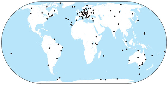
    ly 2009, determined from the data of more than 100 globally well-distributed tracking stations in the IGS network (see Figure 4). A good global distribution of observing sites is extremely important for orbit determination and even more so for the clock determination. Until early in 2008, the GLONASS clock determination suffered from gaps in the global tracking network, which had severe impact on the clock estimates. If tracking gaps cause an interruption of the carrier-phase tracking of a GNSS satellite, the clock estimates are basically reset and a jump will occur. The size of the jump is delimited by the accuracy of the code (pseudorange) observations, that is, at the 1-meter level, or 3 nanoseconds in clock terms.

    We may state that today orbit and clock determination for the GLONASS satellites may be based on a truly global tracking network of high-quality geodetic–type receivers. This significant improvement is due to the efforts of many IGS station managers and their institutions.

    Figure 3. Number of sites in the IGS network providing GLONASS data, used for orbit determination at CODE.
    Figure 3. Number of sites in the IGS network providing GLONASS data, used for orbit determination at CODE.
    Figure 4. Current distribution of IGS combined GPS and GLONASS tracking stations.
    Figure 4. Current distribution of IGS combined GPS and GLONASS tracking stations.

    GLONASS Constellation

    After reaching a full orbit constellation of 24 satellites in early 1996, the GLONASS constellation degraded rapidly due to Russia’s economic difficulties following the break-up of the Soviet Union coupled with the short lifetime of the GLONASS satellites. Since 2002, the GLONASS constellation has slowly but surely been rebuilt (see Figure 5). Currently, there are 21 active modernized GLONASS (GLONASS-M) satellites, which have a significantly longer lifespan compared to the original satellites. Additionally, there are two reserve satellites on orbit.

    Figure 5. Development of the GLONASS satellite constellation since 1982.
    Figure 5. Development of the GLONASS satellite constellation since 1982.

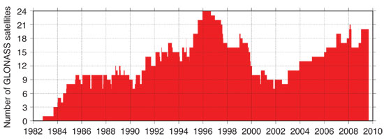
    Russia intends to have a full 24-satellite constellation in place by the end of 2010. To achieve this goal, two more triple-satellite launches are planned, one in August and one in November. The November launch could include a new type of GLONASS satellite, GLONASS-K. The GLONASS-K version is a lighter, unpressurized spacecraft, with a design lifetime of 10 years. In addition to the legacy frequency-division-multiple-access signals, it will transmit code-division-multiple-access signals and use an additional frequency band overlapping with the GPS L5 band.

    Orbit and Clock Accuracy

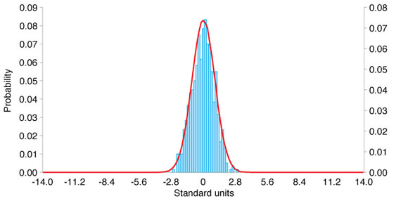
    The developments of both the GLONASS tracking capabilities of the IGS station network as well as the steady increase in the number of GLONASS satellites has had a positive influence on the accuracy of the GLONASS orbits and clocks. It also has significantly increased the interest in the GLONASS system. The enhancement of the IGS GNSS tracking network from an almost purely European network to a truly global network between 2008 and now has had a significant impact on the quality of the GLONASS orbits and clocks. To show the effect on the quality of the GLONASS orbit estimates, we look at the difference between two independent consecutive solutions spanning 24 hours from 0 to 24 hours GPS Time. We compare the “midnight point” of both solutions, that is, the solution at the end of one day (or arc) and the beginning of the next day (or arc). This will give us a worst-case estimate for the orbit quality because typically the orbit is less accurate at the boundary of the orbital arc compared to the middle of the orbital arc. We have analyzed these orbit differences for all GPS and GLONASS satellites separately for four half-year time spans using the routine IGS GNSS solutions from ESOC. The differences are computed in three different satellite-orbit-related directions: radial, along-track, and cross-track. The times spans are:

    • January to June 2008 (6 months)
    • July to December 2008 (6 months)
    • January to June 2009 (6 months)
    • July to December 2009 (6 months)

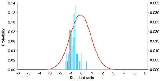
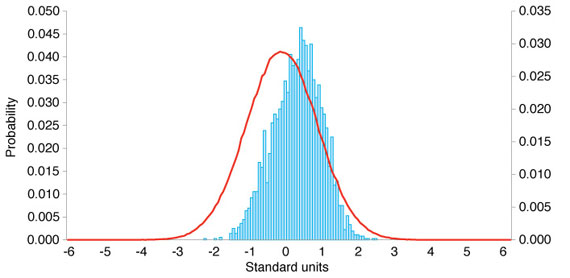
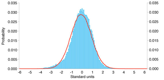
    The results are shown in Figure 6. For the GPS satellites, we cannot see any improvement over time. The quality of the GPS orbits is excellent at the 25- to 35-millimeter level for all three components.

    Figure 6. Evolution of GPS and GLONASS orbit quality from January 2008 to December 2009.
    Figure 6. Evolution of GPS and GLONASS orbit quality from January 2008 to December 2009.

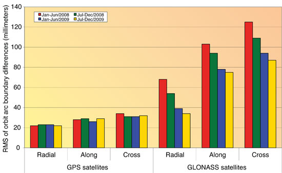
    Remember, we are looking at the worst-case differences here. For GLONASS, we can see a significant improvement over the four time spans. Early in 2008, the orbit quality was at the 120-millimeter level (cross-track), which has improved significantly to the 85-millimeter level. It is important to note that no processing changes were made during this time interval, and that the improvements are thanks to the improvements in the station tracking network and the GLONASS satellite constellation.

    The clock quality is more difficult to assess, but over the timeframe of 2008 to 2009 we have noticed that the clock estimates of the GLONASS satellites have become complete. In 2008, with the still-far-from-global tracking network, there were many gaps in the tracking of the GLONASS satellites. This means that at some epochs no stations were tracking a GLONASS satellite. Such gaps cause jumps in the satellite clock estimates, because the carrier-phase observations become discontinuous, and these jumps are at the 1-meter (3-nanosecond) level. With the improvements of the IGS GNSS tracking network, the GLONASS tracking is now complete and clocks for all epochs are estimated. A comparison of the clocks of the two analysis centers that provide estimated clocks for the GLONASS satellites shows an agreement at the 80-picosecond level, which is only slightly worse than the agreement between the GPS clocks. Significant biases at the few-hundred-nanosecond level exist only in the GLONASS clocks because of receiver internal frequency-dependent delays. The ESOC GNSS orbit and clock products are, however, perfectly suited for precise point positioning using either GPS, GLONASS or, even better, both GNSS simultaneously. It should be noted that since February 2010, the ESOC IGS clock products are now sampled at 30 rather than 300 seconds, which further enhances their suitability.

    Conclusions and Outlook

    The IGS has promised to become a GNSS service by changing its name in 2005, more than four years ago. Meanwhile, the GLONASS satellite constellation as well as the IGS GNSS tracking network have matured and are practically complete. For the IGS to become a true GNSS service, a substantial number of the analysis centers should provide GNSS contributions to all IGS products: final, rapid, ultra-rapid, and real-time. These products should come from performing a rigorous combined analysis of the observations of all active GNSS satellites. It is expected that over the next two years, we will see a significant increase in the number of true GNSS solutions within the IGS, a very positive development for the GNSS world.

    Within the IGS, the analysis centers CODE and ESOC are leading the GNSS efforts. CODE has provided fully consistent GPS/GLONASS products from a rigorously combined processing approach for all IGS products (final, rapid, and ultra-rapid) since May 2003, or for seven years. Since the beginning of 2008, ESOC has followed this good practice for its final products, and in February 2010 ESOC started to produce rapid and ultra-rapid GNSS products. A unique feature of the ESOC products is that they include the clocks for the GLONASS satellites, even with a sampling rate of 30 seconds for the final products. CODE will add GLONASS clocks to its IGS products very soon, during the fi
    rst half of 2010. The GLONASS orbit and clock product quality has become comparable to that of the GPS products within the IGS. However, because GLONASS carrier-phase integer ambiguity resolution is difficult, the GLONASS products are and will remain somewhat less accurate than the GPS products.

    The experiences gathered at CODE and ESOC by fully combining the observations from the GPS and GLONASS systems will pave the way for the integration of additional systems and signals within the IGS. Hence, IGS will retain its leading position in providing the reference, in the broadest sense of the word, for all GNSS. In the near future, this means the integration of QZSS and Galileo observations as well as the integration of the new triple-frequency signals from the latest generation of GPS satellites, Block IIF, the first of which was scheduled for launch last month.

    The positive GNSS developments within the IGS will require an update of the IGS combination software to enable a true GNSS combination. The CODE and ESOC analysis centers have indicated that they are interested in taking on this important task of rewriting and enhancing the IGS orbit and clock combination software to make the IGS a true GNSS service.

    Acknowledgments

    CODE is a collaboration among the Astronomical Institute, University of Bern (Bern, Switzerland), the Swiss Federal Office for Topography (Wabern, Switzerland), the Bundesamt für Kartographie und Geodäsie (Frankfurt am Main, Germany), and the Institut für Astronomische und Physikalische Geodäsie of the Technische Universität München (Munich, Germany).

    The authors are very grateful to the IGS and its numerous contributors for providing the global GNSS tracking data network.


    TIM SPRINGER received his Ph.D. in physics from the Astronomical Institute of the University of Bern (AIUB) in 1999. He has been a key person in the development of the Center for Orbit Determination in Europe (CODE), one of the IGS analysis centers, located at AIUB. Since 2004, he has been working for the Navigation Support Office (OPS-GN) at the European Space Operations Centre (ESOC) of the European Space Agency (ESA) in Darmstadt, Germany. In this group, he has led the development of the new ESOC GNSS software, which is used for most GNSS activities at OPS-GN, including GIOVE-A and -B analyses.

    ROLF DACH received his Ph.D. in geodesy at the Institut für Planetare Geodäsie of the University of Technology in Dresden, Germany. Since 1999, he has been working as a scientist at AIUB, where he is head of the GNSS research group. He oversees the development of the Bernese GPS Software, used at CODE for activities in the frame of the AIUB IGS analysis center and elsewhere.


    FURTHER READING

    • GLONASS Status and History

    Russian Space Agency’s Information–Analytical Center website: www.glonass-ianc.rsa.ru.

    “Renovated GLONASS: Improved Performances of GNSS Receivers” by A.E. Zinoviev, A.V. Veitsel, and D.A. Dolgin in Proceedings of ION GNSS 2009, the 22nd International Technical Meeting of the Satellite Division of The Institute of Navigation, Savannah, Georgia, September 22–25, 2009, pp. 3271–3277.

    “Other Satellite Navigation Systems” by S. Feairheller and R. Clark, Chapter 11 in Understanding GPS: Principles and Applications, 2nd edition, edited by E.D. Kaplan and C.J. Hegarty, published by Artech House, Boston, 2006.

    “GLONASS Performance, 1995–1997, and GPS-GLONASS Interoperability Issues” by G.L. Cook in Navigation, Vol. 44, No. 3, Fall 1997, pp. 291–300.

    “GLONASS Review and Update” by R.B. Langley in GPS World, Vol. 8, No. 7, July 1997, pp. 46–51.

    • The International GNSS Service

    “The International GNSS Service in a Changing Landscape of Global Navigation Satellite Systems” by J.M. Dow, R.E. Neilan, and C. Rizos in Journal of Geodesy, Vol. 83, No. 3-4, March 2009, pp. 191–198, doi:10.1007/s00190-008-0300-3; erratum: Vol. 83, No. 7, July 2009, p. 689, doi: 10.1007/s00190-009-0315-4.

    “GNSS Processing at CODE: Status Report” by R. Dach, E. Brockmann, S. Schaer, G. Beutler, M. Meindl, L. Prange, H. Bock, A. Jäggi, and L. Ostini in Journal of Geodesy, Vol. 83, No. 3-4, March 2009, pp. 353–365, doi:10.1007/s00190-008-0281-2.

    The International GNSS Service: Any Questions?” by A.W. Moore in GPS World, Vol. 18, No. 1, January 2007, pp. 58–64.

    IGS Central Bureau website. IGS FAQ, Site Guidelines, data and product access information, and network details are available: http://igscb.jpl.nasa.gov

    • Benefits of Multi-GNSS

    “The Benefits of Multi-constellation GNSS: Reaching up Even to Single Constellation GNSS Users” by B. Bonet, I. Alcantarilla, D. Flament, C. Rodriguez, and N. Zarraoa in Proceedings of ION GNSS 2009, the 22nd International Technical Meeting of the Satellite Division of The Institute of Navigation, Savannah, Georgia, September 22–25, 2009, pp. 1268–1280.

    “Assessment of GPS/GLONASS RTK Under Various Operational Conditions” by R.B. Ong, M.G. Petovello, and G. Lachapelle in Proceedings of ION GNSS 2009, the 22nd International Technical Meeting of the Satellite Division of The Institute of Navigation, Savannah, Georgia, September 22–25, 2009, pp. 3297–3308.

    The Future is Now: GPS + GLONASS + SBAS = GNSS” by L. Wanninger in GPS World, Vol. 19, No. 7, July 2008, pp. 42–48.

    • GNSS Signal Anomalies

    “Anomalous Harmonics in the Spectra of GPS Position Estimates” by J. Ray, Z. Altamimi, X. Collilieux, and T. van Dam in GPS Solutions, Vol. 12, No. 1, January 2008, pp. 55–64, doi:10.1007/s10291-007-0067-7.

  • The System: First IIF Satellite Speeds into Orbit


    At press time, GPS spacecraft IIF-1 was set to be launched May 27 from Cape Canaveral Air Force Station in Florida. This first of a new generation of satellites will travel quickly — instead of taking several days to reach its orbital slot, the new satellite should make the journey in three-and-a-half hours.

    The new IIFs will broadcast the operational civil L5 signal, intended for safety-of-life applications. It will be compatible with Galileo, GLONASS, and QZSS, with the goal to be interoperable as well. L5 will transmit at a higher power than current civil GPS signals, with wider bandwidth and lower frequency that may enhance indoor reception.

    IIF-1 caught its breathless ride aboard a Delta 4 rocket from the United Launch Alliance, a joint venture of Lockheed Martin and Boeing, formed in late 2006.

    Earlier GPS satellites rode on smaller Delta 2 rockets that, although reliable, did not possess the oomph to place space vehicles directly into the orbiting constellation, 11,000 miles high. Delta 2s put satellites into highly elliptical orbits looping from as low as 100 miles above Earth at perigee to the 11,000-mile apogee. At a strategic point, a solid-fuel kick motor attached to the satellites pushed them into position for circular orbit on high.

    The more powerful Delta 4 will shoot the IIFs directly into their destination slots. Future IIF launches may also use similarly equipped Atlas 5 rockets. The next IIF satellite, GPS IIF-2, could rise aboard an Atlas 5 as early as November.

    The IIF generation, manufactured by Boeing for the U.S. Air Force, is designed not only to broadcast the new civil L5 signal, but have a longer design life of 12 years and faster processors with more memory. “These next-generation satellites provide improved accuracy through advanced atomic clocks, a more jam-resistant military signal, and a new civil signal that benefits aviation safety and search-and-rescue efforts,” said Craig Cooning, vice president and general manager, Boeing Space and Intelligence Systems.

    “GPS IIF will increase the signal power, precision, and capacity of the system, and form the core of the GPS constellation for years to come,” said Air Force Col. David Madden, GPS Wing commander.

    A total of 12 IIF satellites will make their contribution to getting the new L2C and L5 signals closer to operational capability before the GPS III generation takes over, beginning with a 2014 launch.

    As the first spacecraft in the GPS IIF series, GPS IIF-1 underwent stringent and comprehensive testing following shipment to the launch site in February. Tests included verification of key satellite functions as well as end-to-end system testing to verify operations between the satellite and the ground control segment at Schriever Air Force Base in Colorado.

    Commands were sent from Schriever to GPS IIF-1 at Cape Canaveral to turn on payloads, reprogram processors, and verify interoperability with user receivers and equipment, both civil and military.

    Launch of the satellite, originally scheduled for May 20, was delayed four times because of various technical problems.


  • Out in Front: Brussels Calling

    The European Commission rang up the other day, concerned that a recent column contained misperceptions about the Galileo Open Service Signal-in-Space Interface Control Document (ICD). I replied that if misperception exists, it is shared by at least some in industry. Though the EC has abandoned a plan to charge for licenses, its requirement for a free license and continued talk of patents on the Galileo signal dampen industry enthusiasm for making Galileo receivers, at least in North America.

    Herewith, some Brussels counterpoint. “In the previous [ICD] there were some patents characterizing the signal, that could not be commercially exploited. The new publication completely removes these. We now propose a licensing agreement that aims to eliminate any barrier in the wide exploitation of the asset. Both licenses [research and manufacture] are based on non-discrimination. There is no exclusive basis, and they are absolutely free of charge. Furthermore, there is no geographical limitation.

    “Regarding the duration of the license, we are assuming 10 years. We believe this is a proper timeframe, considering the lifecycle investment of this sector. A patent can be enforced for 20 years. The patents that we own are already about five or six years old. If you add 10 years, you almost get to the end.

    “We ask companies to provide us with information on the use of these patents: whether they are used for high-precision receivers, for testing purposes, and so on. We ask for an update on a yearly basis, for information on the intended use. The only purpose is to have a good grip on the marketing, to guarantee a traceability of market needs, to interpret its evolution in a fast-changing context, and therefore enable the Commission to closely follow and support customer needs. In case a manufacturer will develop some patent on top of our patents, they have to notify us. That is, I believe, standard practice.

    “It is not our intention to create barriers to access of this signal. Manufacturers have nothing to fear from providing basic information in these licenses. We want to foster innovation and promote competition.

    “It might seem we are a team of lawyers creating problems where there should not be any. I am an aerospace engineer, not a lawyer.

    “[Complaints] could be more a point of perception. In concrete terms, we are not much different [than GPS]. We want to keep track of what we are giving away for free. We want the widest possible access to the signals. If there are any doubts, we invite manufacturers to contact us directly to work out any misunderstandings.”

    The EC was sincerely surprised to learn of discontent with the process and the patents, and hopes to have further dialog with all manufacturers.

    I was puzzled by the patents: why were they taken in the first place? It’s as if you had drawn a line in the sand, from which you now feel unable to back away, even though you might like to, and it’s clearly the best idea. The EC maintains these date from the public-private partnership effort, where intelllectual property rights were (IPR) were for the private sector a non-negligible form of revenue. Since funding has shifted to public money, “the situation has changed, and we have modified our approach.”

  • Part 2: The Origins of GPS, Fighting to Survive

    Part 2: The Origins of GPS, Fighting to Survive

    Five Challenges, One Key Technology, the Political Battlefield — and a GPS Mafia

    Part 2 of a Two-Part Story. Read Part 1 here.

    0610By Bradford W. Parkinson and Stephen T. Powers, with Gaylord Green, Hugo Fruehauf, Brock Strom, Steve Gilbert, Walt Melton, Bill Huston, Ed Martin, James Spilker, Fran Natali, Joe Strada, Burt Glazer, Dick Schwartz, Len Jacobson, AJ Van Dierendonck, and others.

    GPS Phase I program approval meant that the real work could begin. The conclusion of a two-part history, told by the people who made it.


    By January 1974, the GPS program at the Joint Program Office (JPO) was well underway. With only about 30 officers, the workload was enormous. Fortunately, the Aerospace cadre of about 25 also made extraordinary contributions. In a flurry of activity, the team developed requests for proposals, made top-level specifications, and published initial interface control documents. The work of converting viewgraphs into real hardware, as many know, is an exacting and sometimes painful process.

    Of course there were many challenges, but five of them, principally engineering, stand out as particularly daunting. These were:

    • Defining the specific details of the GPS CDMA signal structure;
    • Developing space-hardened, long-life, atomic clocks;
    • Achieving rapid and accurate satellite orbit prediction;
    • Ensuring and demonstrating spacecraft longevity approaching ten years;
    • Developing a full family of GPS user equipment.

    We discuss each challenge in detail, including the names of those most instrumental in meeting them. The first appearances of their names are highlighted, although if they appeared in Part 1 of this story (May 2010 issue), their names are not highlighted.

    EARLY GPS MANPACK worn by JPO Army deputy Lt. Col. Paul Weber. This photo graced the cover of the first-ever GPS brochure! (Credit: Bradford W. Parkinson and Stephen T. Powers)
    EARLY GPS MANPACK worn by JPO Army deputy Lt. Col. Paul Weber. This photo graced the cover of the first-ever GPS brochure! (Credit: Bradford W. Parkinson and Stephen T. Powers)

    Challenge 1. Defining the specific details of the GPS CDMA signal structure (coherence, acquisition, spreading, communication protocol, structure, error correction, message structure, and so on).

    The selection of the GPS signal structure was broadly confirmed with the tests that were run by program 621B at the White Sands Missile Range with the help of Joe Clifford, Bill Fees, and Larry Hagerman, all from the Aerospace Corporation.

    While the fundamental decision to select CDMA had been made during the Lonely Halls meeting, a vast number of details had yet to be worked out. Fortunately, there were many earlier studies of the signal. Dr. Jim Spilker (then of Philco Ford), who had also written the major reference book on digital communications, authored one of the studies. Dr. Charles Cahn, Nat Natali, Burt Glazer, Ed Martin, and Dr. Robert Gold of Magnavox all made significant contributions. One of the most important details was the decision that the carrier, code, and data of the GPS signal would all be phase-coherent (Figure 1). As discussed later, this decision enabled much of the precision that we now see in advanced GPS receivers.

    FIGURE 1. GPS signals were designed to be all aligned as transmitted, that is, coherent. (Courtesy Misra and Enge, Global Positioning System).
    FIGURE 1. GPS signals were designed to be all aligned as transmitted, that is, coherent. (Courtesy Misra and Enge, Global Positioning System).

    The exact Gold codes family had to be selected from the original family, since Dr. Gold’s technique did not include the natural Doppler shifts. The data message was integrated into both the civil (C/A ) and military (P/Y) signals through inversion of their codes every 20 milliseconds.

    To work out the details of the data message, the JPO had a strong team including Major Mel Birnbaum, Col. Brock Strom, and Capt. Bob Rennard. Outside contractors making major contributions included Dr. Fran Natali, Dr. A. J. Van Dierendonck, and others. Van Dierendonck played a particularly effective role in helping define “GPS time.” This sounds rather mundane, but had some very interesting complexity. Jim Spilker recommended the 1023-bit message length to avoid a correlation problem associated with Doppler shifts (this recommendation was incorrectly attributed in the last issue).

    The data stream came down at 50 bits per second. Through this tiny pipe of information, all the precision of GPS had to pass. It included the space-vehicle orbit-position information (ephemerides), system time, space-vehicle clock-prediction data, transmitter status information, and C/A signal handover time to the P/Y code. Also as a part of the message, ionospheric-propagation delay models were incorporated for the single-frequency user. Further, to aid rapid acquisition of new satellites just rising over the horizon, the ephemerides of all other satellites in the full constellation had to be included. Each digital word had to be defined in terms of scaling, bias offset, and precision in terms of the number of bits transmitted.

    About 95 percent of the GPS message has endured with no changes needed at all. In a few cases, because the newer user equipment is more accurate, greater precision is desirable. It is a great tribute to the brilliant engineers and scientists who designed the signal structure in 1975 that it has endured for 35 years with so little need for modification.

    Some of the JPO Heroes at a "dining-in," a recognition dinner. From left, Major Mel Birnbaum (made many important contributions. He was famous for marathon code reviews that could last 18 hours straight. He hated to miss schedules!); Col. Don Henderson (later Maj. Gen.) second Air Force deputy; Major Ralph Tourino (later Maj. Gen.), Program Control; Lt. Col. Ken Juvette. director of procurement; and LCdr. Joe Strada, a key leader in the extensive test program. (Credit: Bradford W. Parkinson and Stephen T. Powers)
    Some of the JPO Heroes at a “dining-in,” a recognition dinner. From left, Major Mel Birnbaum (made many important contributions. He was famous for marathon code reviews that could last 18 hours straight. He hated to miss schedules!); Col. Don Henderson (later Maj. Gen.) second Air Force deputy; Major Ralph Tourino (later Maj. Gen.), Program Control; Lt. Col. Ken Juvette. director of procurement; and LCdr. Joe Strada, a key leader in the extensive test program. (Credit: Bradford W. Parkinson and Stephen T. Powers)
    Credit: Bradford W. Parkinson and Stephen T. Powers
    Credit: Bradford W. Parkinson and Stephen T. Powers

    Challenge 2. Developing space-hardened, long-life, atomic clocks (qualified for the upper Van Allen Belt, with 4- to 5-year lifetime requirement for individual clocks).

    In 1966, both the Air Force and the Navy recognized that developing a precise, stable time-base for generating the one-way (passive) navigation ranging signal in the satellite was essential. Cesium atomic clocks had been invented, demonstrated, and offered for commercial sale by the middle of the 1950s, before the Space Age. The major commercial issues with these clocks were that they tended to be bulky, power-hungry, and not hardened against space radiation. To address that problem, rubidium atomic clocks, noteworthy for their small size and low power requirements, were developed. Still, the issues of mechanical and radiation hardening as well as temperature sensitivity had to be resolved before they could be used in space.

    The 621B/Woodford/Nakamura study of 1964/66 called for atomic clocks in the satellites in at least seven places. The study advocated a technology program to space-harden existing clock technology. Unfortunately, the Air Force chose not to pursue a space atomic-clock technology program.

    However, the Naval Research Laboratory (NRL) did institute a program in 1964. It pursued the technology for stable clocks with a series of satellites that have already been discussed. The first Timation satellite, launched in May 1967, carried a quartz clock. Not surprisingly, the frequency varied substantially with satellite temperature. The second Timation satellite also contained a quartz clock as well as a temperature controller and showed improved operation, but the results still fell short of those necessary for a GPS satellite. The third satellite in the series had not been launched before the Pentagon approved GPS development in December 1973. In any case, Timation 3 was designed to carry two slightly upgraded, off-the-shelf commercial rubidium clocks.

    Qualification Model of the first GPS atomic clock, built by Rockwell International working directly with Efratom, a small German company. (Credit: Bradford W. Parkinson and Stephen T. Powers)
    Qualification Model of the first GPS atomic clock, built by Rockwell International working directly with Efratom, a small German company. (Credit: Bradford W. Parkinson and Stephen T. Powers)

    Based on the progress that NRL had made, during the Lonely Halls meeting the JPO decided to commit to atomic clocks in the first operational GPS satellites. This third Timation satellite was renamed NTS-I and came under the newly formed Joint Program Office for GPS. The satellite was launched on July 14, 1974, as a part of the GPS program. However, the ineffective attitude-stabilization system caused varying sun angles and hence, significantly varying temperatures, masking any careful evaluation of the rubidium performance.

    The GPS space-based rubidium atomic clock technology was derived from a unit produced by Efratom, a small company initially based in Germany. The geniuses behind this creative device were Ernst Jechart and Gerhard Huebner.

    By the summer of 1974, a satellite contractor, Rockwell International (RI), had been selected to build the GPS operational satellites. Included in the program direction by the JPO was a separate development of rubidium clocks for the satellites as an alternative to the NRL cesium clock effort, in case the NRL effort faltered. Hugo Fruehauf of Rockwell had independently discovered and contacted Efratom, the company that NRL was working with, although his interaction was totally independent of that of the NRL. In addition, Fruehauf’s relationship with Efratom was simplified because of his fluency in German, since Jechart did not speak English, and Efratom had just established an office in Southern California near the Rockwell developers. Figure 2, a page from the original Rockwell proposal, shows the excellent ground test data at both 1000 seconds and at 24 hours.

    Figure 2. Test results for the Rockwell proposed GPS space-hardened prototype atomic (rubidium) clock, based on the Efratom commercial clocks. (Credit: Bradford W. Parkinson and Stephen T. Powers)
    Figure 2. Test results for the Rockwell proposed GPS space-hardened prototype atomic (rubidium) clock, based on the Efratom commercial clocks. (Credit: Bradford W. Parkinson and Stephen T. Powers)

    On realizing that the small Efratom company would be incapable of producing a radiation-hardened, space-qualified rubidium oscillator, RI’s GPS satellite program manager Richard Schwartz created a teaming relationship with them, which included his chief engineer, Hugo Fruehauf, plus Dale Ringer, Dr. Chuck Wheatley of Rockwell’s Autonetics Division, and Efratom’s Werner Weidemann. With heroic efforts, this team built a space-qualified clock in time for the first GPS launch in February 1978.

    Meanwhile, the NRL-sponsored development of a cesium clock by FTS ran somewhat behind schedule. Their cesium clock was not available for the first three GPS satellite launches. The first NRL hardened clock was included on the fourth GPS satellite; unfortunately that unit failed after 12 hours of operation because of a power-supply problem. As a result, the only operating clocks on the first four GPS satellites were those developed by the Joint Program Office through its contractor Rockwell International. The decision to proceed to full-scale development for GPS, called DSARC 2, was made before any NRL-developed clocks had become operational.

    That said, the NRL-sponsored FTS cesium clocks were available for later satellites, and performed extremely well. Later Block II GPS satellites carried two rubidium-frequency standards made by Rockwell and two cesium-frequency standards (primary source, Frequency and Time Systems; secondary sources, Kernco and Frequency Electronics Inc., on selected vehicles). Figure 3 summarizes the early clock program.

    Figure 3. Earliest satellite-clock technology developments, culminating in the last row: four Rockwell satellites with Rockwell-developed rubidium clocks. (Credit: Bradford W. Parkinson and Stephen T. Powers)
    Figure 3. Earliest satellite-clock technology developments, culminating in the last row: four Rockwell satellites with Rockwell-developed rubidium clocks. (Credit: Bradford W. Parkinson and Stephen T. Powers)

    In spite of NRL’s development difficulties, GPS users owe a debt to the lab for its pursuit of this technology. Clearly GPS would not have performed so well without space-hardened atomic clocks. It was the apparent NRL progress that strengthened the argument. The support of Ron Beard of NRL in this joint effort has been invaluable to the program over many years. More than 450 atomic frequency standards have now flown in space. By far the greatest user has been GPS.

    Challenge 3. Achieving rapid and accurate satellite orbit prediction, to within a few meters of user ranging error (URE) after 90,000 miles of travel.

    Since the GPS system architecture had upload stations only on U.S. soil, the satellites were out of sight for many hours, making accurate prediction of their orbits essential. To achieve the expected positioning accuracy, the orbit prediction had to contribute less than a few meters of ranging error after 90,000 miles of travel. Achieving this standard was a major challenge in the early days of GPS. Such a prediction must account for the complications of Earth pole wander, Earth tides, general and special relativity, the noon turn maneuver of the satellite, solar and Earth radiation, and the reference station’s location. Figure 4 gives an example of the problems of polar wander.With roughly a 400-day period, this effect had an amplitude of many tens of feet. While this wander has to be included in the GPS orbit-prediction model, fortunately GPS is the major technique to measure it.

    Another, usually unrecognized feature is that the monitor stations only use the GPS signal for ranging. In other words, they are passive, rather than using the usual technique of that era, two-way ranging. The reference receivers were of a special design, developed by Jim Spilker’s company, STI. They successfully received the first signal from the Rockwell/ITT satellite (NDS-1) on March 5, 1978, after its launch on February 22, 1978.

    Fortunately, the Transit program had pioneered precise orbit prediction and had taken these effects into account. Its Astro/Celeste program, developed by Bob Hill and Dick Anderle at the Naval Surface Weapons Center in Dahlgren, Virginia, batch-processed the measurements taken by the reference stations. Unfortunately, this processing would take too long to provide the most up-to-date predictions.

    A new scheme was devised that included partial derivatives of prediction relative to reference-station measurements. A.J. Van Dierendonck applied his knowledge of filters to help lead development of these calculations, which allowed a modified (linearized) Kalman filter to be used for near-real-time optimal prediction. Bill Fees of Aerospace, Walt Melton of General Dynamics, and Sherm Francisco of IBM, among others, implemented these techniques. The initial master control and upload stations were located at Vandenberg Air Force Base, since moved to Schriever Air Force Station; a backup master control station has been re-established at Vandenberg.

    Figure 4. Motion of the Earth’s spin axis must be included in the measurement parameters for GPS satellite location. The broadcast ephemeris is adjusted to include this effect, so the user need not make further adjustments. (Courtesy of International Earth Rotation and Reference Service). (Credit: Bradford W. Parkinson and Stephen T. Powers)
    Figure 4. Motion of the Earth’s spin axis must be included in the measurement parameters for GPS satellite location. The broadcast ephemeris is adjusted to include this effect, so the user need not make further adjustments. (Courtesy of International Earth Rotation and Reference Service). (Credit: Bradford W. Parkinson and Stephen T. Powers)

    Challenge 4. Ensuring and demonstrating spacecraft longevity approaching 10 years (the issue was GPS affordability)

    The issue was simply that sustaining a constellation of 24 satellites would be prohibitively expensive if the satellites did not have long lives. Again, the Air Force/621B study by Woodford and Nakamura in 1966 focused on the problem: “The most specific change in satellite technology is the increase of mean time before failure (MTBF). MTBFs on the order of 3 to 5 years can now be considered feasible.”

    The problem is easily illustrated in Figure 5. The light blue line shows the trade-off between average satellite lifetime, L, and the required number of satellites per year for a 24-satellite constellation. GLONASS, the Russian system competing with GPS, has the experience shown in the upper white box. With satellite lifetimes averaging two to three years (or less), GLONASS has a corresponding requirement for eight to 12 satellite launches per year. Only a very wealthy country can sustain such a launch program.

    Figure 5. The imperative for long satellite lifetimes. (Credit: Bradford W. Parkinson and Stephen T. Powers)
    Figure 5. The imperative for long satellite lifetimes. (Credit: Bradford W. Parkinson and Stephen T. Powers)

    The red oblong illustrates the U.S. GPS experience, which requires only two to three launches per year. Also shown is the initial experience of GPS during Phase I. The first 10 GPS satellites reached an average age of 7.6 years, with #3 and #10 exceeding 9 years. This is an enormous credit to Rockwell International and in particular the program manager Richard Schwartz. He had excellent system engineering support from Andy Codik. The JPO satellite division was intially led by Major Gaylord Green and later by Maj. Doug Smith, with help from Capt. Jack Henry.

    Three factors are key to long-lived satellites:

    • Designs with carefully selected redundancy (for example, clocks, power amplifiers),
    • Enforcing a rigorous part-selection program including the de-rating of parts (must be class S. or equivalent),
    • Testing as you fly and insisting on a detailed analysis of all failures.

    Figure 5 also illustrates why the Timation clocks could not be used as prototypes for the GPS program. In general, their maximum lifetimes were approximately one year. Clearly their designs needed greater maturation.

    The demonstrated lifetimes were essential to passing the next milestone, DSARC II, which allowed GPS to proceed to full-scale development.

    Challenge 5. Developing a full family of GPS user equipment that capitalized on the digital signal (leading to inexpensive digital implementation) and spanned most fundamental military uses, as well as demonstrating civilian cost feasibility.

    The last, but certainly equally difficult of these five engineering challenges, was the development of nine different types of GPS user equipment. Recognize that a major part of the challenge was to stuff the real-time digital software processing into the relatively primitive digital computers of that era. Table 1 summarizes the development of user equipment:

    Data: Bradford W. Parkinson and Stephen T. Powers
    Data: Bradford W. Parkinson and Stephen T. Powers


    All of the sets performed well within specification. They were characterized, however, by large size and heavy power demands. Magnavox, under the technical direction of Vito Calbi, produced the largest variety of user equipment. It was a subcontractor to General Dynamics, who reported directly to the JPO. At Aerospace, Frank Butterfield was a gifted contributor, particularly skilled at practical antenna design.

    The Generalized Development Model (GDM) reciever, developed by Rockwell Collins Group, was the largest of the sets, created for a specific purpose: to demonstrate the ultimate jam resistance for GPS user equipment. It attained performance better than 100 db jamming-to-signals ratio (J./S) in actual flight test. The GDM receiver achieved this by integration with inertial components, directional antennas, and shading with the aircraft body. Such a receiver can fly directly over a 1 kW jammer at 4,000 feet and not be affected. The original GDM program manager at the USAF Avionics Lab was Maj. Roger Brandt.

    The Rockwell Collins Generalized Development Receiver (GDM). This advanced receiver achieved more than 100 dB of anti-jam in actual flight tests. (Credit: Bradford W. Parkinson and Stephen T. Powers)
    The Rockwell Collins Generalized Development Receiver (GDM). This advanced receiver achieved more than 100 dB of anti-jam in actual flight tests. (Credit: Bradford W. Parkinson and Stephen T. Powers)

    The single-channel manpacks were large and clumsy, but they operated very well. The payoff created by the CDMA signal is illustrated with the 12-channel, single-chip modern implementation, shown in the bottom picture. This contemporary chip’s accuracy is much better than any of the equipment produced during Phase I.

    Developing test environment and analysis setup was almost as challenging as the user equipment. Lt. Col. Val Denninger, Maj. Darwin Abbey, and Lt. Cdr. Joe Strada led this very successful effort. While most testing took place at Yuma Proving Ground, test sites were also located in San Diego and elsewhere.

    <strong>Left:</strong> 1978 single-channel (sequential) Manpacks, two types by Magnavox and Texas instruments. Batteries alone weighed much more than current military handsets. <strong>Right:</strong> The second JPO deputy, Col. Don Henderson (left), and Aerospace program manger Ed Lassiter (right). <strong>Bottom:</strong> A modern 12-channel (parallel) Atheros chip receiver with more capability. (Credit: Bradford W. Parkinson and Stephen T. Powers)
    Left: 1978 single-channel (sequential) Manpacks, two types by Magnavox and Texas instruments. Batteries alone weighed much more than current military handsets. Right: The second JPO deputy, Col. Don Henderson (left), and Aerospace program manger Ed Lassiter (right). Bottom: A modern 12-channel (parallel) Atheros chip receiver with more capability. (Credit: Bradford W. Parkinson and Stephen T. Powers)

    The Most Fundamental GPS Innovation

    The CDMA (spread-spectrum or PRN) modulation used for passive ranging is clearly the most fundamental innovation of GPS. This signal enabled four-dimensional positioning for the user without requiring an atomic clock in the user equipment. The Russian GLONASS (the other, partially-operational global navigation satellite system) also used spread-spectrum passive ranging, but resorted to a frequency-separation scheme (FDMA, frequency-division multiple-access) that has proven inferior in actual use.

    The innovative design of this CDMA signal has enabled all of today’s precision applications for GPS. It is currently common for inexpensive GPS receivers to simultaneously receive signals from more than 10 satellites, yet all of these signals are being broadcast on exactly the same frequency. In fact, the number of signals that can be received is virtually unlimited using the spread-spectrum CDMA approach. Using a routine processing algorithm, the user, receiving more than four signals, has an instantaneous position that is more accurate than that using four satellites alone. This robustness includes a technique to ensure integrity of the GPS solution. The method, called receiver-autonomous integrity monitoring (RAIM), isolates a rogue satellite that is not operating properly, to ensure integrity of the GPS solution.

    Another technique, called carrier tracking, is enabled with the coherence of the code and the carrier broadcast in this signal. When coupled with some form of differential GPS operation, the result is relative positioning accuracy that is unprecedented — frequently better than a millimeter. For example, surveyors can now routinely resolve three-dimensional position to this accuracy. Even common user equipment can make use of the coherence of the signal. The receiver accomplishes this by employing the so-called Hatch/Eschenbach filter that uses the reconstructed carrier signal to smooth the code-transition measurement that greatly decreases the noise of the raw code measurement.

    The processing gain in the GPS CDMA signal has been enhanced by deep integration with inertial navigation components. This has enabled the demonstrations of very high interference rejection by such receivers. Dale Klein and Ed Copps of Intermetrics Corp. were major contributor
    s to the integration of GPS with inertial measurement units for the Magnavox high-performance military receivers.

    Side-Tone Ranging. The competing side-tone ranging signal structure offered by NRL in the 1970 Easton patent had a fundamental flaw. If the signals were broadcast at the same frequency, they would interfere with each other. On the other hand, if they were broadcast on different frequencies, the user equipment would require a separate analog front end and tracking loops for each signal. In addition, each channel would have its own time-delay bias that would probably vary with temperature of the user equipment. A study by Magnavox also noted that the side-tone ranging signal could be easily spoofed; it was not clear how to encrypt such a signal. The final problem was that the signal was fundamentally an analog type and would have not been able to take advantage of modern digital signal processing. As a result, the receivers would be more complex and expensive.

    The Air Force 621B/Aerospace and Magnavox studied the CDMA signal structure extensively after the 621B Woodford/Nakamura study was completed in 1966. Bob Gold of Magnavox had, in 1967, invented the technique to select acquisition codes that were mathematically guaranteed to not look alike (were uncorrelated). Early in the program, the JPO hired Dr. Jim Spilker, a recognized worldwide authority on digital signal processing, to contribute to this effort. Another worldwide expert, Charlie Cahn of Magnavox, was also a major contributor to the signal design. As mentioned previously, the details of the signal required the efforts of many people.

    By 1969, the CDMA signal was being used in many communication applications. Adapting this signal for navigation raised the questions that were posed in an earlier section. It is hard to believe today the issues surrounding its use had to be addressed in 1970. It is to the great credit of Program 621B that it built the receivers and ran the series of tests at White Sands Missile Range that had earlier resolved all the major issues surrounding the signal structure. This irrefutable evidence allowed the JPO team to confidently choose this signal during the Lonely Halls meeting in September 1973. Great credit must go to Bill Feess who worked tirelessly to complete the analysis that demonstrated 5-meter accuracy in those White Sands tests.

    CDMA-Enabled Applications

    The distinction between the Timation side-tone ranging and the 621B CDMA signal is critical to understanding the origins of GPS. The Air Force CDMA signal was different in essential and fundamental ways from the Easton side-tone ranging modulation. Three examples of precise three-dimensional applications, not achievable with side-tone ranging, illustrate the subsequent success of the 621B digital CDMA signal.

    Aircraft Blind Landing. In 1992, the Federal Aviation Administration (FAA) sponsored Stanford’s development and demonstration of the first Category III (blind landing) system in a commercial aircraft; the effort was led by Clark Cohen and developed by a group of Stanford students under the supervision of Brad Parkinson. The only sensor for both position and attitude was GPS. The carrier-tracking receiver was a derivative of a Trimble receiver; it relied on the CDMA signal structure for both accuracy and integrity. (See Figure 6.)

    Figure 6. Results of first blind landing tests using GPS alone, 110 landings with a commercial Boeing 737. (Credit: Bradford W. Parkinson and Stephen T. Powers)
    Figure 6. Results of first blind landing tests using GPS alone, 110 landings with a commercial Boeing 737. (Credit: Bradford W. Parkinson and Stephen T. Powers)

    Robotic Farm Tractor. Using similar technology, a different group of Stanford students in the same lab demonstrated the first precision GPS-controlled robotic farm tracker. Again, the capability was enabled by the GPS CDMA signal. The John Deere Company sponsored this effort, which has now expanded into a worldwide market of more than $400 million per year.

    Robotic farm tractor developed at Stanford with support from John Deere company. Student leader Mike O’Connor and colleague Tom BeLl shown. Tracking test at 5 meters/second, with worst error around 3 inches! Now a $400M/year market. (Credit: Bradford W. Parkinson and Stephen T. Powers)
    Robotic farm tractor developed at Stanford with support from John Deere company. Student leader Mike O’Connor and colleague Tom BeLl shown. Tracking test at 5 meters/second, with worst error around 3 inches! Now a $400M/year market. (Credit: Bradford W. Parkinson and Stephen T. Powers)

    Earth Crustal Monitoring. A third example of the power of the CDMA signal is precise survey, focused on Earth movement and crustal tracking (Figure 7). The original GPS surveying receivers were pioneered by Phil Ward at Texas Instruments and Charlie Trimble at Trimble Navigation, among others.

    Figure 7. Continuous observation of earth crustal motion with a precision of better than a millimeter: distributed slip on Kilauea volcano, Hawaii. (Credit: Bradford W. Parkinson and Stephen T. Powers)
    Figure 7. Continuous observation of earth crustal motion with a precision of better than a millimeter: distributed slip on Kilauea volcano, Hawaii. (Credit: Bradford W. Parkinson and Stephen T. Powers)

    Summary. Many technologies came together to make GPS operational, none more revolutionary than the signal structure demonstrated by 621B at White Sands, and selected by Parkinson during the Lonely Halls meeting. Virtually all high-precision uses of GPS depend on the characteristics of this signal.

    Credit: Bradford W. Parkinson and Stephen T. Powers
    Credit: Bradford W. Parkinson and Stephen T. Powers


    More on GPS Origins

    The fundamental basis for the GPS design was clearly the Woodford/Nakamura and subsequent studies undertaken by 621B, not the system outlined by NRL in the Easton patent. More than 500 million current users have overwhelmingly confirmed the value of the selected technique using a minimum of four-satellite passive ranges and the CDMA signal. If each GPS user had to employ an atomic clock, the price of most GPS receivers would be prohibitive. The value of a four-dimensional solution for users has also been irrefutable. Had GPS followed the blueprint of the NRL patent, it is reasonable to say that almost all system uses, military as well as civilian, would have been fatally compromised. Further, had the Easton side-tone ranging signal been selected, broadcasting 30 satellites on the same frequency, as GPS does today, would have created an undecipherable electromagnetic jumble.

    Summarizing Easton’s Patent. We earlier mentioned the NRL/Easton patent for the Timation design. It is important to summarize that invention and its relationship to the actual GPS design. A few people have written that Roger Easton “invented” GPS. As stated, Easton did have a competing concept that he had developed at NRL. In October 1970, four years after the completion of the secret, seminal system study by Woodford and Nakamura, Easton applied for a patent, “Navigation System Using Satellites and Passive Ranging Techniques,” that was granted on January 29, 1974 (U.S. 3,789,409). A careful reading of the patent, available on the web, reveals the following:

    • The technique described by Easton clearly calls for a synchronized “extremely stable oscillator” at the user station. Elsewhere he states: “would typically be controlled by an atomic clock.” This less-capable method of navigating was examined in the Woodford/Nakamura study, four years before Easton’s patent application, and is definitely not the technique chosen by GPS.
    • The patent advocates the use of a passive ranging technique, whose description occupies most of the patent, with multiple frequency tones, not the CDMA technique of GPS that had already been studied by 621B. Before the patent was issued, 621B had already built prototype GPS CDMA receivers, flown them at the White Sands range, and demonstrated three-dimensional accuracies of about 5 meters. The Easton passive-ranging technique, commonly called side-tone ranging (STR), had been included in a 621B analysis of alternatives. STR was rejected because of poor resistance to interference or spoofing, and the inab
      ility to broadcast all satellites at the same frequency without destructive self-interference.
    • Both the description and the accompanying diagram in the patent clearly refer to two-dimensional navigation, using lines of position. To extend this to three or four dimensions was not mentioned. Such extension would probably only be possible if the satellites all broadcast on different frequencies, which would have made extremely high-precision positioning (as attained by the actual GPS design) infeasible.

    Thus, it is correct to state that the Easton patent did not, in any way, represent the actual GPS design in at least these three fundamental aspects.

    Further Transit Contribution. In 1974, after the first phase of GPS had been approved, the Transit program requested funds to upgrade the Transit signal structure to the same passive ranging technique (CDMA) being planned for GPS. The program’s purpose was to use Transit signals to track Trident missile testing launches in broad ocean areas. Air Force Col. Bradford Parkinson (director of the GPS Program), Dr. James Spilker (Stanford Telecommunications Inc.), and Jack Klobuchar (Air Force Cambridge Research Laboratory) responded with a technique for substituting GPS signals, with a translated frequency relayed to the ground to track those missile tests.

    After three Pentagon briefings on the proposed alternative technique, Dr. Bob Cooper of the DoD concluded that the GPS signal would be used. Included was a decision to add two more satellites to the Phase I development of GPS to accommodate the Trident launch window. As a result, $66 million was transferred from the Navy to the USAF GPS program. The benefit to the fledgling GPS program was enormous. This greatly expanded the test time for GPS, and also reduced the risk, since no spare satellites had been approved for the program. While the Trident program was somewhat unhappy with the loss of funds and control, it immediately unleashed the creativity of Johns Hopkins University Applied Physics Laboratory and successfully met the Trident missile test tracking requirements.

    GPS JPO Innovations

    GPS was the first DoD program directed to be managed as a Joint Service Development Program. This new approach, conceived by Dr. Currie, led the GPS program to be designated a JPO or Joint Program Office. As a result, there were deputy program managers assigned from the Navy (Cdr. Bill Huston), Army (Lt. Col. Paul Weber), Marine Corps (Lt. Col. Jack Barry), and Defense Mapping Agency (Paul Frey), as well as the customary Air Force deputy (initially Lt. Col. Steve Gilbert, later Lt. Col. Don Henderson). Rather than use these well-qualified people from other services simply as liaisons, they were each assigned specific programmatic responsibilities.

    At the first major program review at Andrews Air Force Base, Parkinson called the convening general’s attention to the fact that he was leading a joint program, and with the general’s indulgence he had invited his deputies from the other services to attend. Since attendance by other services at Air Force program reviews was unheard of, this drew a gasp from the roughly 200 Air Force officers attending. The JPO approach truly broke new ground in intra-service cooperation.

    At the JPO. Frank Butterfield of Aerospace, Col. Parkinson, and Cdr. Bill Huston, deputy JPO director from the U.S. Navy, in the early 1970s. A model of a Phase I GPS satellite stands on the table between the latter two. (Credit: Bradford W. Parkinson and Stephen T. Powers)
    At the JPO. Frank Butterfield of Aerospace, Col. Parkinson, and Cdr. Bill Huston, deputy JPO director from the U.S. Navy, in the early 1970s. A model of a Phase I GPS satellite stands on the table between the latter two. (Credit: Bradford W. Parkinson and Stephen T. Powers)

    Parkinson had entreated the Federal Aviation Administration to also send a deputy. The public response by the FAA deputy administrator for development was: “We don’t want GPS, we don’t need GPS, and if it is ever deployed, we will never use it.” Throughout this period, Glen Gilbert (sometimes called “the father of air traffic control”) was a strong and early advocate for FAA use of GPS. It took many years for the FAA to accept his views. Obviously times change; the current relationship between the FAA and the GPS Program Office is excellent, fostered by Col. Dave Madden and his FAA counterpart Leo Eldredge.

    JPO as Prime Contractor. The JPO cadre served as the prime or integrating activity for the whole program. Gen. Schultz almost fired Parkinson when he proposed this. The general had expected him to hire a separate commercial integrating contractor. After Parkinson explained that the major interfaces between the three segments — satellite, ground control, and user equipment — were the signals, Gen. Schultz acceded to the plan. This pioneering aspect was critical because it ensured that all aspects of the system would be under the direct purview and control of the JPO.

    Award and Incentive Fees. The use of innovative procurement awards for the contractors was very new in DoD in 1974. Beginning with the satellite contract, the JPO made extensive use of new forms of positive rewards for the contractor, including incentives for on-orbit performance. Gaylord Green pioneered this activity with skills developed as a project officer in the Advanced Ballistic ReEntry Systems Program (ABRES) program office. Incentives were applied to virtually all the other contracts as well, and seemed to have a very positive effect.

    Normally the Space and Missile Systems Organization (SAMSO) procurement office, which was independent of the JPO, would have been reluctant to approve such radical new ideas. Fortunately, Parkinson carpooled with another colonel who was head of SAMSO procurement and a breath of fresh air. This attitude was exemplified by a sign at eye level as you left the procurement director’s office: “Nothing would be done at all if a man waited until he could do it so well that no one could find fault with it.” (It turns out this came from remarks by Cardinal John Henry Newman.) With that attitude, the SAMSO office approved almost all of the JPO’s “wild” procurement innovations. Many of these innovations are now routine.

    Changes. The Air Force provided a high-level spec for the satellite that defined the signal structure, the power on the ground, the frequencies, the orbit, and the amount of weight the booster could put into that orbit at apogee. The JPO left it up to the contractor to design a satellite that could meet those requirements. The key point is the JPO never changed the requirements, which kept GPS on course with minimum cost increases for the devlopment.

    Refurbished Atlas F Booster. Today, up to half the cost of a satellite on-orbit is the cost of the booster to place it there. While the costs were perhaps not proportionally so large in 1977, they still could consume large pieces of a program’s budget. Luckily, the United States had mothballed much of its liquid-fuel ballistic missile force during that period. The JPO chose to use refurbished Atlas Fs as boosters, saving many millions of dollars. Some have suggested this idea originated with NRL. While NRL may have also been using them, both Parkinson and Green came from the ABRES program where refurbished Atlas Fs were already employed. Thus, the decision made in the Lonely Halls meeting was based on knowledge the JPO already had, which included additional steps the ABRES had taken to improve the reliability of the booster. (See Figure 8).

    Figure 8. Refurbished Atlas-F booster characteristics. Col. Parkinson and Maj. Green brought this concept from previous use on the USAF ABRES program. (Credit: Bradford W. Parkinson and Stephen T. Powers)
    Figure 8. Refurbished Atlas-F booster characteristics. Col. Parkinson and Maj. Green brought this concept from previous use on the USAF ABRES program. (Credit: Bradford W. Parkinson and Stephen T. Powers)

    A Motto. Emblazoned on a prominent wall in the JPO was a sign that read:

    “The mission of this Program Office is to

    • Drop 5 bombs in the same hole
    • and build a cheap set that navigates
    • and don’t you forget it!”

    By distilling the JPO mission into one succinct motto, the program intended to provide a guide for all its actions. If a decision fundamentally helped achieve that mission, it was probably the right one.

    The Political Battlefield. Political battles in the Pentagon are often brutal and unforgiving. The fundamental reason is that the budget is always viewed as a zero-sum game. One program’s money comes at another program’s expense. GPS was a system that sprang from the space development community (“the Space Weenies”) and had virtually no champions from the operational components. Unlike current DoD satellite programs, there were no explicit formal requirements for the new system and hence little official status. Parkinson spent many trips to the operating forces to explain the value of precision weapon delivery. Between skepticism and deafness, GPS survival was always extremely uncertain. The Air Force generally opposed its deployment, even after the extensive tests of 1978–80 had clearly demonstrated that GPS was, by far, the best blind-bombing system ever conceived.

    Fortunately, there were some key supporters of GPS who overcame that resistance. They were affectionately called the GPS Mafia. The most important member of this unchartered group was Malcolm Currie, whose efforts were discussed earlier. His powerful number-three position at the Pentagon gave him the authority to force funding decisions on the uniformed military. At least one general officer was extremely upset with Parkinson over his relationship with Dr. Currie, and gave him a public tongue-lashing over the issue during a chance encounter in a Pentagon corridor. Dr. Johnny Foster, whom Mal Currie replaced, was another early supporter of the program.

    USAF Col. Steve Gilbert, the original deputy program manager for GPS in Los Angeles, was a tireless, heroic contributor. Later on he played a critical role, fighting the battles within the Pentagon as the Air Force Program Element Monitor (PEM). His next position was as the GPS representative in the Office of the Secretary of Defense. While there, Steve fought back repeated challenges that would have canceled GPS in the early 1980s. Without his efforts, GPS almost certainly would never have happened.

    Other members of the GPS Mafia were Lt. Col. Paul Martin (the original GPS Program Element Monitor), Brig. Gen. Hank Stelling (RDS in Pentagon), and Cols. Brent Brentnall and Emmitt DeAvies (DDR&E representatives).

    The users of GPS owe all of these supporters a real vote of thanks. As the Duke of Wellington said about the battle of Waterloo, “It was a near-run thing.”

    Fortunately, GPS supporters prevailed, and the two Iraq wars have made all branches of the military believers in the value of the system, although they sometimes regard it as magic. A combat Army colonel in Iraq was reportedly asked what he thought of satellite systems to help him fight. His response:

    “I don’t need any (expletive) space systems. My GPS and my Iridium comm give us everything we need.”

    GPS really is a stealth utility.

    Thoughts on the Future

    There are now many additional or improved satellite systems on the horizon. American GPS has heretofore only offered a single, clear navigation signal for civil users. That is rapidly changing. Two more frequencies and a number of additional signals will be available from the next two generations of U.S. satellites. Other countries are also working hard to follow the GPS lead. Figure 9 depicts some of these new systems.

    Figure 9. Upgrades of GPS (only current operational civil signal; next generation, four new civil signals at two new frequencies), GLONASS (next generation, four new civil signals at two new frequencies) and new international navigation satellite systems (Galileo, four new civil signals to appear at two new frequencies; finally, Compass) are on the near horizon. The plethora of signals will enable improved accuracy and integrity. This will lead to new applications. (Credit: Bradford W. Parkinson and Stephen T. Powers)
    Figure 9. Upgrades of GPS (only current operational civil signal; next generation, four new civil signals at two new frequencies), GLONASS (next generation, four new civil signals at two new frequencies) and new international navigation satellite systems (Galileo, four new civil signals to appear at two new frequencies; finally, Compass) are on the near horizon. The plethora of signals will enable improved accuracy and integrity. This will lead to new applications. (Credit: Bradford W. Parkinson and Stephen T. Powers)

    An international common navigation signal called L1C has been accepted and almost completely defined. It will broadcast on the same 1575 MHz frequency as the current GPS civil signal. It will be of the same type (CDMA) as the original GPS signal, although it will have significant enhancements to increase precision and accuracy. If the engineering is done properly, this signal should be interchangeable for all GNSS systems that support civilian use. The positioning, navigation, and timing (PNT) community will benefit enormously by having all of these signals available. Again, the key enabling decision was the CDMA signal structure defined by 621B and tested at White Sands.

    We will mention one CDMA-enabled application with a large market potential. This is the use of multiple GNSSs (up to 50 satellites) in automobiles for lane guidance and car separation. During times of low visibility, freeways are notorious for multi-vehicle collisions. We believe the technology will be in hand to greatly reduce these tragedies. The new application would involve cooperative navigation with cars in the vicinity all tied together in a communication grid. GPS-measured velocity is almost a forgotten aspect of the system, yet it can be accurate to much better than 0.1 meters per second. If two cars in the vicinity of each other can know both relative position and relative velocity, collision probabilities can be easily assessed and avoidance actions quickly and automatically recommended.

    This is just a glimpse of the future. We believe many other new or improved applications will be enabled by future deployments.

    Summary

    Just as a building is not invented, GPS was not the product of any single invention. GPS as a system was an innovation enabled by many antecedent technologies and concepts. Some were brand new in application, or had to be adapted to their role in GPS, for example the CDMA signal technique. In making those system selections, the final design was the product of the entire JPO team, whose roots went back to many of the greatest institutional sources of innovation in the country.

    The two most critical foundations were:

    • The comprehensive study done by Jim Woodford and Hideyoshi Nakamura for USAF/621B in 1964/66, exploring virtually all alternative ranging techniques from satellites, both active and passive, and calling for atomic clocks in the satellites. In particular, the four-dimensional 621B concept of using “four in view” was analyzed and became the bedrock of the GPS design, ensuring that the user could make do with a simple crystal clock.
    • The selection and demonstration of the CDMA passive ranging signal by 621B at White Sands. These tests confirmed four-satellite, single-frequency operation and proved that such operation obviates the need for an atomic clock in each GPS user set.

    These directly led to the systems architecture decisions made in the Lonely Halls meeting. Also essential were finding workable solutions to the five critical challenges:

    • Defining the specific details of the GPS CDMA signal structure
    • Developing space-hardened, long-life, atomic clocks
    • Achieving rapid and accurate satellite orbit prediction
    • Ensuring and demonstrating spacecraft longevity
    • Developing a full family of GPS user equipment.

    In tracing the origins, the first navigation satellite program, the Transit program of APL, should be singled out. Working under contract to the Navy’s Nuclear Submarine Program, APL pioneered the dual-frequency technique to calibrate ionospheric delay errors as well as the painstaking development of an accurate orbit-prediction program. Both early efforts were essential to the ultimate success of GPS.

    Also important was NRL’s push to harden frequency standards for use in satellites. While the JPO rejected Easton’s navigation technique, NRL’s apparent clock progress, by 1973, convinced the decisionmakers at the Lonely Halls meeting to commit to including atomic clocks in the first prototype, Rockwell-built GPS satellites. While it is ironic that no clock with NRL heritage was operational on the first four GPS satellites, the NRL’s persistence finally paid off with the introduction of its cesium beam clocks on an equal footing with the Efratom/Rockwell-designed rubidium clocks later, during GPS Phase II.

    Throughout this article, many of the contributors to the early definition, development, and testing of GPS have been named. Certainly many others have also been inadvertently left out. In closing we would like to sincerely thank the scores of engineers who assembled the first-of-a-kind demonstration system.

    As a stealth utility, one pervasive accolade is that GPS is now taken for granted. People throughout the world now expect to know exactly where they are and what time it is.

  • GPS, GLONASS, and SBAS Webinar Follow-up

    Normally, my column following a webinar is dedicated to Q&A follow-up from the webinar. However, immediately following the April 22 webinar, I traveled to Phoenix, Arizona, to attend the ACSM/GITA conference, which I wrote about earlier this month.

    This column is dedicated to answering questions I didn’t address during the webinar. Also, I always find the results from the polls I conduct during the webinar very interesting.

    Poll #1: Have you or your work crews had to stop or alter your work pattern due to the lack of GPS satellites?

    Total votes: 128, Yes: 73%, No: 27%

    Gakstatter comment: This is consistent with other polls I’ve conducted regarding GPS satellite availability. The new GPS 24+3 configuration will help mitigate this problem. Read more about the new GPS 24+3 configuration in a three-part series I wrote earlier this year.


    Poll #2: How often do you upgrade your GPS equipment?

    Total votes: 113

    Gakstatter comment: There’s no clear pattern here except to say that 46% of the users wait until at least 3 years before they consider upgrading their GPS equipment. That makes sense to me.


    Poll #3: Does any of your GNSS equipment utilize GLONASS?

    Total votes: 115, Yes: 39%, No: 61%

    Gakstatter comment: When considering the result of this poll, keep in mind that there are very few “mapping-grade” receivers that are designed to utilize GLONASS. For example, there are very few, if any, sub-meter receivers that utilize GLONASS, primarily due to the lack of correction sources. SBAS doesn’t support GLONASS, DGPS (radiobeacon) doesn’t support GLONASS, and most CORS do not support GLONASS. Only recently did OmniSTAR begin supporting GLONASS. I think this trend will continue, although I doubt that SBAS or DGPS (radiobeacon) will support GLONASS in the foreseeable future.

    Poll #4: Does any of your GNSS equipment utilize SBAS (WAAS/EGNOS/MSAS) as a primary source of corrections?

    Total votes: 111, Yes: 60.5%, No: 39.5%

    Gakstatter comment: This poll result doesn’t surprise me. Given that SBAS corrections are widely available, free of charge, reasonably accurate, and require no action by the user, it makes a lot of sense they are being used.

    Following are some of the questions that were posed by the audience during the webinar:

    Question #1: I am not sure, but when you say you’re “pushing” something out to us, it sounds like your trying to “push” something on us. Just a comment.

    Gakstatter: I’m sorry about the webinar-speak. When I say “pushing the next slide,” that means I’m changing slides. I may change the way I say this. Thanks for your comment.

    Question #2: Can you correct GLONASS signals with WAAS or other real-time technologies?

    Gakstatter: WAAS (or any SBAS) doesn’t support GLONASS. Neither does DGPS (radiobeacon). This doesn’t mean that GLONASS measurement can’t be used, but you’ll be using uncorrected measurements to augment SBAS-corrected measurements. A case where it may be useful is when you’re mapping in an environment where there are a lot of trees. You might only have four GPS satellites visible that are being corrected via SBAS. In that scenario, there might be value in utilizing measurements from GLONASS satellites just to improve the PDOP, even though the GLONASS measurements are uncorrected.

    Question #3: Do you feel manufacturers will begin to release lower-end mapping-grade GPS receivers with L2C and L5 functionality in the future?

    Gakstatter: Yes, I do, but it will be a few years before there are enough satellites broadcasting an L5 signal. I think what you’ll end up seeing are inexpensive L1/L5 receivers (Galileo doesn’t support L2). They will not only be able to provide mapping-grade sub-meter, decimeter) but also RTK accuracies (cm-level). Since L2C and L5 are open civil signals, you won’t see the patent blocks that restrict competition for L1/L2 receivers like you do today.

    I’m not saying L2C will not be supported at all. I think there will be L1/L2C/L5 receivers, but I think you’ll see L1/L5 on lower-end receivers.

    Question #4: There is apparently some degradation of accuracy when using GPS and GLONASS for RTK. Have there been any rigorous studies quantifying this that you are aware of?

    Gakstatter: I’m not sure I’d say I believe there is degradation in accuracy, but I wouldn’t count on GLONASS to improve accuracy. The value of GLONASS is improving productivity. Since it adds several satellite signals to the solution, it effectively eliminates GPS “brown-out” periods so RTK can be used 24/7. There was a rigorous study released by The Survey Association in the UK. The report focused on network RTK. They tested both GPS and GPS+GLONASS. You can download a copy of the report here.

    Question #5: Does using GLONASS-capable receivers shorten the observation time required for fast-static points?

    Gakstatter: My first thought is yes since generally more observables equates to shorter occupation time, but I would check with the manufacturer and follow their recommendations. Honestly, I’ve only used fast-static with GPS-only receivers so I don’t have any personal experience with your scenario.

    Question #6: When is GLONASS-K launch scheduled? When can we receiver a valid CDMA signal?

    Gakstatter: The first GLONASS-K satellite is scheduled for launch later this year. I haven’t seen a launch schedule beyond that. A representative from the Russian Space Agency is scheduled to present at the Institute of Navigation (ION) GNSS conference in September, so I’ll probably learn more at that point. However, it’s a lengthy process. It’s not just a matter of launching satellites. There are many other variables and unknowns such as the control segment and user equipment compatibility. I think it’s safe to say that we are a few years away from having a minimal GLONASS satellite constellation broadcasting CDMA.

    Question #7: The visibility plots show one extra satellite in the “after” plots. Was that intentional? I would have expected there to be an improved number of satellites visible when one more was added to the plotted constellation.

    Gakstatter: Good catch. In the “after” scenario, I set SVN-49 healthy, which it is currently not. The reason I did this was because SVN-49 is in an important slot in the 24+3 configuration. The status of SVN-49 is still undecided, but if they decide to not set it healthy they will move another satellite to take its place in the 24+3 configuration. If I would have kept it unhealthy in the “after” scenario, it would have only s
    hown a 24+2 configuration. Clear as mud?

    Question #8: Is 24+3 the solution to the blackout problem from now to 2014 stated by the GAO Report from last year?

    Gakstatter: The definition of the 24+3 configuration had been around before the GAO Report. Personally, I don’t think the GAO Report had anything to do with 24+3. The 24+3 configuration just helps optimize the current satellites in orbit, whereas the GAO Report addresses the attrition of GPS satellites outpacing the addition of GPS satellites.

    Question #9: Cellphone question: Is the move to 24+3 likely to degrade indoor GPS coverage – fewer peak sats => lower probability of seeing 4+ sats indoors?

    Gakstatter: Interesting question. My first thought is probably so, although I think it would be a temporary problem. Assuming Galileo keeps pushing forward, that would be a big help for cellphone users, both indoors and outdoors.

    Question #10: GPS Satellites are getting beyond the design life…is the USA behind schedule in satellite updates?

    Gakstatter: GPS satellites have been unbelievably reliable. PRN-24, the oldest operational satellite, has been in operation since August 30, 1991. Since they have been so reliable, there hasn’t been as much pressure to launch GPS satellites. Prior to the 24+3 initiative, the minimum guaranteed constellation was 24 satellites. It costs $50-60 million to build each GPS satellite and another $150-200 million to launch it. With the GPS constellation hovering around 30 satellites these past few years, and government budgets tightening, I think it’s clear that the pressure to save money has resulted in a more relaxed launch schedule.

    The delay in the Block IIF satellite (the first one being launched this week) was not a result of the above, but rather technical and program management mis-steps. The GAO Report was particularly critical of the IIF development.

    Question #11: Do you see any future for ground-based free systems such as those broadcasting corrections in LF/MF radio, like the Coast Guard broadcasts?

    Gakstatter:
    There is an interesting debate between DGPS (what you mention) and SBAS. The DGPS infrastructure has been in place and working reliably for mariners for better than a decade. Funding for DGPS seems solid for marine navigation, but less stable for inland-based applications (like the U.S. NDGPS system). I think the future of DGPS for mariners is solid for the next 10 years. Once there is a full constellation of satellites broadcasting GPS L5, the value of DGPS will be questioned.

    Question #12: Will WAAS, EGNOS, etc. be needed after L1/L5 receivers can measure the iono effects themselves?

    Gakstatter: I think it comes down to integrity. If the L1/L5 combo can deliver integrity that safety-of-life applications require (such as aviation), then one has to question the value of SBAS. My gut feeling is that the L1/L5 combo can’t and that some sort of augmentation will be needed to attain the integrity level required.

    Question #13: What are your thoughts concerning Compass? Do you feel this will eventually be applicable for public use as part of a functioning GNSS?

    Gakstatter: Compass is the GNSS wildcard. Since the Chinese aren’t particularly forthcoming with their plans, it’s hard to say. But I’m not sure that matters. With a full constellation of GPS, GLONASS (CDMA), and Galileo satellites in the future, that’s around an average of 25+ satellites in view at any one time during the day. If China doesn’t play well with others in a timely fashion, the user community won’t care what Compass brings to the table.

    Question #14: If my current GPS receiver is not ready for L2C and L5, do I have to buy a new GPS or I can upgrade software/firmware later so that I can still use it?

    Gakstatter: You’ll have to trade-in. Some might be upgradable to L2C, but L5 is a different story. It’s a completely different frequency. That affects the receiver as well as the antenna.

    I wasn’t able to address all of the questions here, so look for more in the next newsletter. Particularly I’ll cover some discussion about reference frames, SBAS and L5.

    Look for announcements in the next day or so about the Block IIF GPS satellite launch. It’s scheduled for Friday, May 21. It’s a new era with the first GPS satellite to broadcast an operational L5 signal.

    Thanks, and see you next time.

    Follow me on Twitter at http://twitter.com/GPSGIS_Eric

  • Carrier-Phase Anomalies Detected on SVN-48

    By Brady O’Hanlon, Mark L. Psiaki, Paul M. Kintner Jr., and Steven P. Powell

    Anomalous behavior of the L1 C/A-code carrier phase has been detected on PRN07/SVN-48. The anomalies are sudden step-like changes of phase by about 10 degrees/5 millimeters. These steps are followed by negative steps of the same magnitude that restore the original phase time history. These anomalous square pulses have been observed with durations as short as 0.1 seconds and as long as 600 seconds. They can occur about once a minute or be absent for hours.

    These anomalies could be of consequence for some GNSS applications. For precise monitoring of differential total electron content (TEC), the magnitude of this anomaly is the same order as the signals of interest. Precise point positioning (PPP) systems seek to achieve CDGPS accuracy without direct double-differencing. The lack of double-differencing would allow any L1 C/A carrier phase anomaly to directly affect the PPP solution.

    This behavior was detected when testing a dual-frequency software receiver that processes the GPS civilian signals on L1 and L2. The anomaly was first noted when calculating carrier-phase-based TEC:

    where bTEC is a bias term that occurs in the phase-based calculation. Figure 1 shows a plot of the resulting TEC, after removal of its mean value, with six square-edged pulses that range in duration from 0.1 to 590 seconds, with the first a short one at t = 48 seconds. The last pulse starts at 710 seconds and ends at 1300 seconds. In all cases, the anomaly consists of a positive step change in TEC followed some time later by a negative step change of identical magnitude. Step magnitudes in the range 0.04 to 0.07 TEC units have been observed.

    Figure 1. Square pulses on phase-based TEC due to L1 C/A carrier phase anomalies.

    Tests were performed to ascertain whether the anomalies were caused by the L1 signal, the L2 signal, or a combination of the two. Additional tests ruled out receiver malfunction as the cause of the anomalies.

    Observation of detrended L1 and L2 carrier-phase time histories quickly revealed that the anomalies occur on the L1 carrier phase. The detrended L1 C/A carrier phase shows square-edged pulses corresponding to times, magnitudes, and signs of the TEC anomalies, but the detrended L2C carrier-phase plots show no such pulses. Figure 2 shows a typical detrended L1 C/A beat carrier-phase anomaly.


    Figure 2. A typical detrended L1 C/A beat carrier-phase anomaly.

    Extensive tests checked whether the anomalies may have been caused by the receiver. They were initially discovered using a digital storage receiver of raw RF front-end samples followed by off-line software receiver processing. Such carrier-phase anomalies could result from signal glitches in the RF front-end’s mixing chain, from data recording anomalies in the RF front-end samples, or from errors in the software receiver code. The former two possibilities were ruled out by two means. One was to process signals from other satellites for the same RF samples. Mixing problems or data sample problems would cause similar anomalies on all GPS signals, but other GPS signals were found to be free of anomalies. Additional tests used simultaneous data collection by two digital storage receivers spaced 700 meters apart and using different RF front-end hardware. Both receivers showed identical anomalies at identical times.

    Software receiver code errors were ruled out by employing two independent sets of receiver processing code, one developed in MATLAB, the other in C. These two pieces of software were developed independently by different individuals and run independently by their developers. Both showed identical anomalies.

    A final check used a different receiver, the NovAtel GSV4004B. Figure 2 plots its detrended L1 C/A carrier phase along with that of the C-based Cornell software receiver. Both show the same anomaly. Thus, the anomalies appear to be caused by the SVN-48 transmitter.

    All observations were made from roof-mounted antennas in Ithaca, New York. The anomalies were first observed on March 24, 2010 and were observed again on April 1, 5, 7, and 29, and as late as May 13th. For one period of several hours on May 11, no anomalies occurred. Other Block IIR-M satellites have been monitored briefly, but without finding any similar anomalies to date: SVNs 58, 55, 57, 49, and 50.

  • INRIX’s Crowd-Sourced Traffic Network Surpasses 2 Million Vehicles

    INRIX announced its Smart Driver Network has grown to more than 2 million GPS-enabled vehicles giving drivers a reliable, real-time view of traffic conditions on more than 260,000 miles of highways, city streets and secondary roads nationwide.

    “Our Smart Driver Network is the largest real-time traffic network in the world. It redefines what it means to deliver truly real-time traffic information,” said INRIX President and CEO Bryan Mistele.

    According to the announcement, more than 40 percent of all State DOTs in the United States rely on INRIX’s real-time traffic information for their daily operations, traveler information services and/or congestion performance measures. New projects in 2010 in 5 states – Texas, Massachusetts, Maryland, Minnesota and Ohio – are using INRIX traffic data and travel times for their planning efforts, statewide 511 systems or dynamic message signs.

    “In just two years, INRIX has grown from providing traffic data for one state agency to powering the daily operations, planning or traveler information services in 21 states and the District of Columbia,” said INRIX Vice President of Public Sector Rick Schuman.


  • ACSM/GITA Conference Coverage

    The annual ACSM (American Congress on Surveying and Mapping) isn’t what it used to be. Attendance was way down and the number of exhibitors is way down. The technical content, however, was still pretty good. In fact, I’ve included links to several videos I recorded at the ACSM/GITA conference.

    This year, the ACSM conference was co-located with the GITA (Geospatial Infrastructure & Technology Association) annual conference. This made the trip worthwhile. By themselves, both conferences are becoming too small for most attendees (and therefore, exhibitors) to attend.

    GITA is a GIS conference targeted at the global geospatial community, but in reality it attracts infrastructure geospatial users such as electric/gas/water utilities and local government.

    This mix of ACSM and GITA is interesting and was a great opportunity for surveyors. While the economy is starving surveyors who are in the typical boundary and land development markets, the GITA crowd, in my estimation, are in dire need of a GIS-versed land surveyor.

    There are many topics that were interesting and I thoroughly enjoyed most of the ones I attended, but there are two points I want to address about this conference:

    1. Surveying/GIS collaboration discussion
    2. Surveying Body of Knowledge discussion

    If I can write fast enough, there is a third I’d like to tackle regarding the Driven By Data discussion. If not in this column, I’m sure I will touch on it in a future column or maybe in my Geospatial Solutions Weekly column.

    Surveying/GIS Collaboration

    One of the major benefits of co-locating the ACSM and GITA conferences is that it gives attendees a chance to mix it up with the “other side.” History has consistently demonstrated that it’s always easier to view the “other side” with a certain level of antipathy from afar. However, when one learns more intimately about the adversary’s intentions and struggles, that antipathy eventually turns towards empathy and appreciation. I recall listening to a US Veteran of World War II talking about fighting the enemy. I’m paraphrasing, but it went something like this:

    “I believed in what we were doing and fighting the enemy was just doing my job. In those circumstances, we were enemies. Under peaceful circumstances, however, we may have been neighbors and we may have even been good friends.”

    Land surveyors and GIS folks should be good friends. They both have a lot to gain from a positive relationship and a lot to lose with an adversarial relationship, with the former standing to lose the most.

    Rudy Stricklin presented a very good session entitled “Professional Land Surveyors and Geospatial Professionals Building Bridges in Arizona.” In the presentation, he describes the process surveyors and GIS folks went through in Arizona to collaborate and find a common ground to work from. I’m not saying I necessarily agree with everything that was presented or enacted in Arizona, but Rudy’s consistent and often used terms like “collaboration” and “inclusive” certainly conveyed the team-building spirit and positive attitude needed to build a long-term relationship. The bridge-building process presented by Rudy is a model that would be difficult to go wrong with in a similar endeavor by another state, province or local/regional government.

    I recorded the presentation in its entirety. It’s in five parts with each being about 10 minutes in length. I suggest listening to the first segment as he paints the broad picture. However, the entire presentation is well worth your time.

    Part 1 – Professional Land Surveyors and Geospatial Professionals Building Bridges in Arizona (9:10 minutes)

    Part 2 – Professional Land Surveyors and Geospatial Professionals Building Bridges in Arizona (9:23 minutes)

    Part 3 – Professional Land Surveyors and Geospatial Professionals Building Bridges in Arizona (9:39 minutes)

    Part 4 – Professional Land Surveyors and Geospatial Professionals Building Bridges in Arizona (9:12 minutes)

    Part 5 – Professional Land Surveyors and Geospatial Professionals Building Bridges in Arizona (9:59 minutes)

    There was also a discussion panel entitled “GIS/Surveying Geospatial Collaboration.” On the panel was Gene Trobia, Arizona State Cartographer, Jack Avis, PLS, and Bill Coleman, PLS. Jack and Bill are both land surveyors who offer GIS services.

    Gene has some great stories about the early ESRI years and GIS challenges. He recalled there were 37 people at the first ESRI User Conference he attended.

    Watch this 85 second description by Gene of the challenge faced by GIS managers explaining why some are myopic.

    I posed a couple of questions to the panel.

    The first was the subject of a National Parcel Database with references to the First American parcel database.

    Part 1 – National Parcel Database discussion (2:26 minutes)

    Part 2 – National Parcel Database discussion (8:36 minutes)

    The second question I posed was how can a small surveying firm that is focused on boundary and mortgage surveys (and is starving) can transition to offering GIS services.

    How Can a Small Surveying Firm Transition to Offering GIS Services (9:55 minutes)


    Surveying Body of Knowledge (BoK) discussion

    • Josh Greenfeld, Ph.D., PLS
    • Earl Burkholder, PLS, PE (New Mexico State Univ)
    • Wendy Lathrop, PLS (Private practice)
    • Joe Paiva, Ph.D., PLS (Geomatics consultant)

    The focus of this presentation/discussion was to define the role (Body of Knowledge) of professional surveyors in the 21st century.

    Why develop a Surveying Body of Knowledge (BoK)?

    According to the committee (the folks above plus Bob Burton, PLS, PE and Bob Dahn, PLS), the Surveying BoK was developed to:

    1. Formulate a scope of the surveying profession.
    2. Promote recognition for the need for college education.
    3. To help surveyors in business development.
    4. To develop a surveying scholarship
    5. To help promote the surveying profession.
    6. To define the distinctiveness of the surveying profession.

    The Surveying BoK Committee has defined the surveying profession to encompass the following disciplines:

    • Positioning
    • Imaging
    • GIS
    • Law
    • Land development

    The discussion was led by Josh Greenfeld with Earl and Joe presenting on Positioning, Josh presenting for Robert Burtch on Imaging, Wendy presenting on Law, Josh presenting on GIS, and Wendy presenting on Land Development.

    Often referred to as the world’s second-oldest profession, it’s ironic that land surveyors are trying to redefine themselves after thousands of years. But, technology has forced them to face reality. I can’t say I wouldn’t do the same thing. I would say, however, that it’s late in the game for this. Of course, hindsight is 20-20, but this effort really should have begun 10 years ago. Someone dropped the ball.

    Regardless, I think they’ve got the right idea. The BoK committee consists of pe
    ople who are highly respected in the surveying profession. The BoK document is not perfect (and they recognize that and are looking for input), but it’s a step in defining the future of the surveying professional.
    I think expanding the horizons of the land surveyor to include the five disciplines (positioning, imaging, GIS, law and land development) is a great idea. This would expand the profession significantly as it would paint a much more current and accurate picture of the knowledge and skillset a student could strive to achieve if they chose surveying as a profession to pursue. A Surveying Body of Knowledge (BoK) doesn’t exist today so it’s difficult to paint a picture and describe the knowledge and skillset much beyond that of boundary surveyor.

    Kudos to the committee for devoting the time and energy to assemble the BoK document. Although I don’t have a link to the detailed Surveying BoK that was handed out at the presentation, click here to view a Surveying BoK paper that Dr. Greenfeld presented at the FIG (International Federation of Surveyors) conference about one month ago.

    However, I want to make what I feel is a very important point

    I mentioned this during the discussion and I’ll write it here. If one of the purposes of this document is to take it and run to the state legislature to have it legally define the land surveyor’s domain (and therefore eliminate others from operating in that space), I would vehemently oppose it. Honestly, I got that weird feeling when Dr. Greenfeld made a comment early in his presentation that one of the Surveying BoK purposes was to be used “to define the distinctiveness of the profession against those who are trying to encroach on our profession [because] there are a lot of cases like this.” In other words, he’d like positioning, imaging, GIS, law (as related to surveying) and land development to be the exclusive domain of the land surveyor. That would be a mistake, a HUGE mistake. After the discussion group, I asked Dr. Greenfeld about this remark. He dismissed the premise with the thought that laws can be changed and that a larger group with more resources could overturn such a law if there was enough dissent.

    The reason I think it would be a huge mistake is because it limits competition. It’s common knowledge that competition breeds innovation. Henry Ford said “you can have any color (automobile) you want, as long as it’s black.” Without competition, you may still be driving a black automobile without air conditioning. Of course, all-out competition is not the answer either. Just like in politics, the right answer is not at either extreme, but somewhere in the middle.

    As a side note, here is a short clip from the audience regarding the importance of communication skills in the education of land surveyors.

    The importance of land surveyor communication skills (4:36 minutes)


    To give you a flavor of the rest of the conference content, following is a partial list of technical presentations at both conferences.

    ACSM:

    • The Surveyor’s Role in the FEMA Flood Insurance Program
    • Hydrographic Surveying
    • Understanding the Statistics Used in GPS Surveying
    • Development, Implementation, and Future of the National Spatial Reference System
    • The Surveying Body of Knowledge
    • The Surveyor’s Role in Boundary Conflict Resolution
    • Introduction to GIS for Surveyors
    • GIS, Geodesy, and the Ghost in the Machine: A Workshop for Surveyors and GIS Professionals
    • Professional Land Surveyors and Geospatial Professionals Building Bridges in Arizona
    • Panel Discussion: Driven by Data: Who Pays? Who Plays?
    • GNSS Technology Update (presented by Yours Truly)
    • The Truth about an RTK Localization/Calibration

    GITA:

    • How the Evolution of GPS is Transforming Surveying and Mapping (presented by Yours Truly along with Pam Fromhertz of NGS)
    • Geospatial Solutions to Address Aging Infrastructure
    • GIS/Surveying Geospatial Collaboration
    • Geospatial Solutions for Preparing and Responding to Natural Disasters
    • Spatial Analysis in a CAD-driven GIS
    • Geodata Creation and Sharing
    • Location, OGC, and the Smart Grid
    • Spatial Law and Policy
    • Building a Facilities Information Infrastructure to Support Public Safety
    • Offshore Wind Energy GIS Development for the Gulf of Maine
    • Haiti, Open Source Mapping, and the Collaborative Environment
    • Phoenix Sky Harbor Airport Enterprise GIS – Managing Signage Infrastructure and Content
    • Streamlined Methods to Collect and Maintain GPS and Attribute Information for Utility Assets


    Lastly, if you’re interested, here’s a link to my “GNSS Technology Update” presentation I made at the ACSM Technical Session.

    GNSS Technology Update

    Thanks and see you next time.


    Follow me on Twitter at http://twitter.com/GPSGIS_Eric


  • Part 1: The Origins of GPS, and the Pioneers Who Launched the System

    Part 1: The Origins of GPS, and the Pioneers Who Launched the System

    Part 1 of a Two-Part Story. Read Part 2 here.

    Cover: GPS World
    Cover: GPS World

    By Bradford W. Parkinson and Stephen T. Powers, with Gaylord Green, Hugo Fruehauf, Brock Strom, Steve Gilbert, Walt Melton, Bill Huston, Ed Martin, James Spilker, Fran Natali, Joe Strada, Burt Glazer, Dick Schwartz, Tom Stansell, and others

    The original system study, the key innovations, and the forgotten heroes of the world’s first — and still greatest — global navigation satellite system. True history, told by the people who made it. Part One of a Two-Part Special Feature.

    The stealth utility: over the past 30 years, a new entity has steadily and stealthily crept into the fabric of worldwide society, creating capabilities and dependencies that did not exist before. This utility is known as the Global Positioning System, or GPS. With more than a billion GPS receivers in use, this stunning achievement has truly revolutionized the way the world functions in the 21st century. Virtually every cell-phone system relies on GPS for timing. Almost every ship and aircraft carries multiple GPS receivers to provide positioning information. Other applications span military targeting, transportation, object tracking, and resource identification. Today, the loss of GPS signals would have catastrophic consequences.

    How did GPS come into being? What technologies were essential to its success? Who developed those technologies? Recently a number of GPS histories have appeared that are very inaccurate on these subjects. Our purpose in writing this account is to set the record straight, and in so doing to give credit to many of the original developers of GPS whose contributions have somehow been forgotten. Throughout this article you will find their names highlighted. Space does not permit us to name the many other individuals who deserve enormous credit for the subsequent refinement and invention of new GPS applications.

    Figure 1 gives a summary view of the history of U.S. satellite-based navigation, particularly GPS. Details of the Russian GLONASS and the European Galileo systems are not included as they arrived later, and generally mimicked the GPS development albeit with their own, locally developed detailed designs.

    Figure 1. The eras of satellite navigation. (Credit: Bradford W. Parkinson and Stephen T. Powers)
    Figure 1. The eras of satellite navigation. (Credit: Bradford W. Parkinson and Stephen T. Powers)
    Dr. Richard Kershner, who led the development of Transit. On his left, young Col. Bradford Parkinson, who led the development of GPS. (Credit: Bradford W. Parkinson and Stephen T. Powers)
    Dr. Richard Kershner, who led the development of Transit. On his left, young Col. Bradford Parkinson, who led the development of GPS. (Credit: Bradford W. Parkinson and Stephen T. Powers)

    This history focuses on the period up to about 1980, when GPS was approved for full-scale development. Between that time and the date that GPS was declared fully operational, April 27, 1995, many additional contributions were made. The system withstood several early attempts by the Air Force to cancel it entirely. Fortunately, those attempts did not succeed, and the Air Force now fully embraces GPS as an essential part of virtually every weapon system in the inventory.

    We call this a tribute to the almost-forgotten people whose intellectual labor and skill initially developed GPS. As we unveil this story, we will point out the original — and critical — system study, the 1966 Woodford/Nakamura Report, that became the essential blueprint for GPS. Many people are unaware of this study since, in its original form, it was classified U.S. Department of Defense (DoD) Secret. It was not declassified until August 1979, more than a year after the first launch of a GPS operational satellite in February 1978.

    We also intend to describe and justify the key innovation that enabled the system. This keystone technology is the GPS code-division multiple-access (CDMA) signal. While CDMA was necessary for GPS success, it was by no means sufficient.

    We will also define and describe the five major original challenges that had to be met to achieve the success that GPS now enjoys; that will come in the second installment of this history, to appear in next month’s issue.

    Mathematician Bill Guier (l) and physicist George Weiffenbach (r), told APL Research Center director Frank T. McClure (c), about their success using Doppler tracking for satellites. “McClure’s brain started going into fast forward,” remembered John Dassoulas. “Knowing the navigational challenges the U.S. Navy faced, McClure said, ‘Well, if you can find out where the satellite is, you ought to be able to turn that problem upside down and find out where you are.’" (Credit: Bradford W. Parkinson and Stephen T. Powers)
    Mathematician Bill Guier (l) and physicist George Weiffenbach (r), told APL Research Center director Frank T. McClure (c), about their success using Doppler tracking for satellites. “McClure’s brain started going into fast forward,” remembered John Dassoulas. “Knowing the navigational challenges the U.S. Navy faced, McClure said, ‘Well, if you can find out where the satellite is, you ought to be able to turn that problem upside down and find out where you are.’” (Credit: Bradford W. Parkinson and Stephen T. Powers)

    GPS Predecessors: Transit

    On October 4, 1957, the entire world was amazed by the launch of Russia’s Sputnik satellite. The American public greeted this event with both apprehension and curiosity. Both the Army and Navy had been quietly working on satellite projects for some years. In an attempt to catch up, the United States had a spectacular failed launch when the Naval Research Laboratory’s (NRL’s) TV-3 crashed on December 6, 1957. On January 31, 1958, the United States Army launched a grapefruit-sized satellite, Explorer 1. The NRL then achieved success with the launch of TV-4, renamed Vanguard-1, on March 27, 1958.

    In 1958, the Applied Physics Laboratory (APL) of Johns Hopkins University employed an extremely competent team of engineers and scientists. Two of those scientists, Drs. William Guier and George Weiffenbach, began to study the orbits of the new Sputnik satellites. The satellites were broadcasting a continuous tone signal. Their velocity relative to the ground created a Doppler shift of that signal that was unique. After some innovative work, Guier and Weiffenbach discovered they could determine the Sputnik’s orbit with a single pass of the vehicle.

    At that point Frank McClure of APL made a very creative suggestion: Why not turn the problem upside down? Using a known satellite position, a navigator could determine his location anywhere in the world after receiving and processing the satellite signal for 15 minutes. His insight became the basis for the Navy’s Transit satellite program, also known as the Navy Navigation Satellite System (Figure 2).

    This pioneering system was developed under the leadership of Dr. Dick Kershner, head of the Space Department of APL. Transit’s main purpose was to provide position updates to the United States submarine ballistic-missile force then under development. These submarines were a major deterrent during the Cold War. Transit was first tested in 1960, and by 1964 the system was fully operational. Under Kershner, APL rapidly mastered the art of building long-life satellites. In fact, two of the vehicles continued operation for more than 20 years.

    Figure 2. The Transit birdcage of operational orbits. (Credit: Bradford W. Parkinson and Stephen T. Powers)
    Figure 2. The Transit birdcage of operational orbits. (Credit: Bradford W. Parkinson and Stephen T. Powers)

    Transit was a relatively small satellite that initially used solar power and gravity-gradient stabilization (Figure 3). It provided a position fix every few hours; fixes took 10 to 16 minutes of exposure of the submarine’s antenna on the surface. It achieved 25-meter accuracy, but only in two dimensions. Further, if the user was moving, accurate velocity measurement was critical: a 1-knot error would produce a 0.2-nautical mile position error.

    All Navy ships could use the system, and in 1967 Transit was offered to the civilian community by Vice President Hubert Humphrey. Magnavox became the principal developer of civil user sets with Tom Stansell as an early expert in the technology.

    Contributions to GPS. The Transit program developed a technique essential for GPS: the use of two frequencies to calibrate the time delay of the radio signal induced by the ionosphere. This dual-frequency technique was incorporated into GPS to attain the highest positioning accuracy. In addition, Transit also pio
    neered the accurate prediction of satellite orbits, another essential GPS technology. Orbit prediction will be highlighted later, as one of the five fundamental challenges that faced GPS system designers.

    In 1974, Transit made a further contribution to GPS development that we discuss in that approximate timeframe.

    Figure 3. A Transit satellite showing the gravity-gradient boom that kept the antennas pointing at the earth. (Credit: Bradford W. Parkinson and Stephen T. Powers)
    Figure 3. A Transit satellite showing the gravity-gradient boom that kept the antennas pointing at the earth. (Credit: Bradford W. Parkinson and Stephen T. Powers):

    Program 621B

    As early as 1962, Dr. Ivan Getting, president of the Aerospace Corporation, saw the need for a new satellite-based navigation system. He envisioned a more accurate positioning system that would be available in three dimensions, 24 hours a day, seven days a week. He had direct access to the highest levels of the Pentagon and was a tireless advocate for his vision.

    Getting’s energy and foresight in the early 1960s were essential to gaining Air Force support to study system alternatives. As a result, the Air Force formed a new satellite navigation program that was later named 621B. Getting’s efforts were recognized in 2002 when he shared the Charles Stark Draper Prize of the National Academy of Engineering with Bradford Parkinson.

    By 1962, engineers at Aerospace, under Air Force sponsorship, were heavily immersed in studying the system aspects of a new navigational satellite system. From 1964 to 1966, Aerospace carried out an extensive, formal system study whose principal authors were James Woodford and Hideyoshi Nakamura, both highly regarded space-systems engineers.

    Their work was summarized as a DoD secret briefing in August 1966. As a result of the classification, it was unavailable to anyone outside the project until 13 years later, in 1979, when it was finally declassified (figure 4).

    The Woodford/Nakamura Report was a complete system study that examined these issues:

    • capabilities and limitations of then-current DoD navigation systems;
    • tactical applications and utility of improved positioning accuracy;
    • comprehensive analysis of alternative system configurations and techniques for positioning, using satellites.

    The report concluded with a set of recommendations for advanced technology development for navigation satellite programs.

    Figure 4. Front page of the seminal GPS system study performed from 1964 to 1966 by USAF 621B Program. Originally classified secret, it was not declassified until after the initial GPS satellite had been launched. This was the essential foundation to the GPS System design. (Credit: Bradford W. Parkinson and Stephen T. Powers)
    Figure 4. Front page of the seminal GPS system study performed from 1964 to 1966 by USAF 621B Program. Originally classified secret, it was not declassified until after the initial GPS satellite had been launched. This was the essential foundation to the GPS System design. (Credit: Bradford W. Parkinson and Stephen T. Powers)

    The detailed analysis of possible passive navigation techniques was extremely important. It pointed out that the most capable passive-ranging design, called triple delta rho, would eliminate the need for an extremely stable clock in the user equipment and would provide three-dimensional positioning. (In this article we use clock, oscillator, and frequency standard interchangeably. The timing community makes some distinctions among these words, but for purposes of this history the distinctions are not particularly important.) This later was selected as the fundamental GPS system concept of ranging to four satellites simultaneously.

    Key conclusions of the 1966 study advocated:

    • passive ranging from the satellites (the issue was which ranging signal to use)
    • atomic clocks in space, and a technology program to develop space hardened atomic clocks
    • further system studies as well as experimental demonstrations.

    Since the full survey of alternative system configurations was extremely important in selecting an optimum system configuration, we reproduce the summary in figure 5. Note that the “Computation Performed by User” is split into two columns. Focus on the columns of the one-way passive ranging techniques with the red outline. Inside, there are two “user boxes,” one with A and one with X. The A shows the user needs an atomic clock. The X shows the user needs only a crystal clock. The option later selected for GPS is designated as G. This technique is the 3Δρ (triple delta rho, or four satellites) that eliminated the need for the user atomic clock, and provided three-dimensional positioning (really four-dimensional since it also captured time).

    In October 1970, more than four years after the completion of this study, Roger Easton of NRL applied for a patent on the two-satellite, ρ-ρ technique (option N) that required an atomic clock for the user and was only two-dimensional. The patent (U.S. 3,789,409) was granted in 1974, a year after the three-dimensional design of the GPS system had already been defined in the Lonely Halls Pentagon meeting to be described later.

    Figure 5. Summary of the alternative satellite-based navigation techniques from the1964–66 USAF/621B study. The most capable option, circled in green, became the basis for the White Sands prototyping and testing, and then evolved into GPS. NRL applied for a patent on the less capable technique (red line) four years after the Woodford/Nakamura Study was completed. (Credit: Bradford W. Parkinson and Stephen T. Powers)
    Figure 5. Summary of the alternative satellite-based navigation techniques from the1964–66 USAF/621B study. The most capable option, circled in green, became the basis for the White Sands prototyping and testing, and then evolved into GPS. NRL applied for a patent on the less capable technique (red line) four years after the Woodford/Nakamura Study was completed. (Credit: Bradford W. Parkinson and Stephen T. Powers)
    Credit: Bradford W. Parkinson and Stephen T. Powers
    Credit: Bradford W. Parkinson and Stephen T. Powers


    More 621B Studies. From 1966 to 1972, program 621B continued with trade-off studies including: signal modulation, user data processing techniques, orbital configuration, orbital prediction, receiver accuracy, error analysis, system cost, and comprehensive estimates of the tactical mission benefits. More than 90 reports completed by USAF/Aerospace during this period remain available in the Aerospace Corporation library.

    PRN or CDMA Signal Structure. Of these studies, the most important were those aimed at selecting the best passive ranging technique for the navigation signal. By 1967, it appeared that the best technique was a variation of a new communications modulation known as CDMA. Pioneering this signal were several outstanding scientists, Dr. Fran Natali and Dr. Jim Spilker (both of Philco-Ford), and Dr. Charlie Cahn (of Magnavox).

    Credit: Bradford W. Parkinson and Stephen T. Powers
    Credit: Bradford W. Parkinson and Stephen T. Powers


    This signal has many names. In addition to CDMA, it is sometimes called spread spectrum, since the energy of the signal was spread over a wide range of radio frequencies. It is also sometimes called PRN or pseudorandom noise because the encoded (and repeated) sequence appears to be random transitions of +1 and -1.

    The name code-division is used because each satellite is assigned its own coded signal. Each was a binary (digital) sequence selected to be uncorrelated with other signals and also uncorrelated with time shifts of the signal itself. The expected, powerful advantage of this technique was that all satellites would broadcast on exactly the same frequency. It would clearly lend itself to digital signal processing. Furthermore, and very important, any time-shifts induced by the receiver for the various satellite signals would be effectively eliminated.

    However, several significant questions concerning CDMA still needed resolution. These included:

    • Could such a signal be easily acquired in the face of time uncertainty and Doppler shifts?
    • Was there a technique to encrypt the military signal so that unauthorized users could not gain access?
    • How would the c
      odes be easily selected to avoid a false lock and also allow additional satellites to be added without interfering with existing satellite signals?
    • Would the anticipated complexity of the receiver drive costs to unacceptable levels?
    • Was the signal resistant to accidental or deliberate interference?
    • Could this signal accommodate communication capability for satellite location, satellite clock correction, and other parameters?

    Fortunately, in 1967 a technique for selecting orthogonal codes was invented by an accomplished applied mathematician, Dr. Robert Gold of the Magnavox Corp. Naturally these are now known as the Gold codes. His solution resolved the third CDMA issue stated above.

    White Sands Tests. To address the remaining issues, the 621B program developed two prototype versions of CDMA navigation receivers (Magnavox and Hazeltine) for testing at the White Sands Missile Range (WSMR). For these initial 1971 tests, 621B arranged four transmitters in a configuration known as the inverted range. (Interestingly, the more capable receiver was the MX-450 that was only on loan from Magnavox.) These transmitters broadcast CDMA signals from locations that were similar to a satellite configuration except that they were broadcast from the ground. For the simulation of satellite geometry, a balloon-based transmitter was also included for the aircraft-landing tests. Al Gillogly of Aerospace spent many hours installing and troubleshooting the test configuration.

    Al Gillogly, Aerospace engineer (left), setting up the critical tests of prototype GPS receivers at WSMR in 1970. (Credit: Bradford W. Parkinson and Stephen T. Powers)
    Al Gillogly, Aerospace engineer (left), setting up the critical tests of prototype GPS receivers at WSMR in 1970. (Credit: Bradford W. Parkinson and Stephen T. Powers)

    By 1972, program 621B had successfully proven the effectiveness and accuracy of the CDMA signal by demonstrating that such a configuration would achieve 5-meter, 3-dimensional navigation accuracy. Much credit for the painstaking analysis of these results should go to Bill Fees of Aerospace who wrote the final detailed test report. These test results answered most of the remaining issues regarding the CDMA signal.

    The tests also confirmed the power of the modulated signal by showing that all satellite signals could, indeed, be received simultaneously on the same frequency. These tests also corroborated the expectation that ranging to four satellites eliminated the need for a highly precise user atomic clock, while still supporting full, three-dimensional navigation. This became an extremely important feature of GPS. If each user had required an atomic-clock class frequency-standard, no inexpensive user equipment could have been produced within the technology horizon visible at that time. This is still true today.

    All this evidence supported CDMA as the passive ranging signal of choice and was available to the Air Force’s 621B team when the system configuration was selected at the September 1973 Pentagon meeting that will be discussed later.

    621B Demo, Operational Differences. From the time of the 1966 Woodford/Nakamura study on, the Air Force and Aerospace advocated the use of atomic clocks in the operational satellites with the modulation also originating in the satellites. There were two significant risks to placing atomic clocks in the satellites: First, the technology readiness risk: no hardened atomic clocks had yet been designed and flown; and second, the political/budgeting risk associated with gaining approval for a development/demonstration program for the full capability. The Air Force developed a plan to reduce both risks.

    In late 1968, the Air Force’s NavSat program in the Plans Office (XR) at the Space and Missile Systems Organization (SAMSO) was redesignated as 621B. All of the various proposals that went forward from SAMSO to Headquarters came henceforth from the 621B office in XR. This included a proposal in early 1972 to deploy a four-satellite demonstration system. This proposal addressed both risks. It would reduce the technology readiness risk in the clocks by launching simple L-band transponders. At the same time, it would save substantial money, thereby reducing the political/budgeting risk.

    QZSS (Credit: Bradford W. Parkinson and Stephen T. Powers)
    QZSS (Credit: Bradford W. Parkinson and Stephen T. Powers)

    In many circles, this proposal was erroneously thought of as 621B because it came from that office, but in fact, the operational concept for 621B never contemplated or advocated using transponders in the final operational system. Transponders had been rejected for the operational system because they could be easily jammed from the ground. Such a jamming signal would overpower the transponder and steal all of the transmitted energy away from the transponded navigational signal. This enemy jamming would shut down the entire system, clearly an unacceptable risk.

    Proposed Initial Constellation. To demonstrate four-satellite, passive ranging capability, 621B had studied a number of orbital configurations, including geo-synchronous and lower inclined orbits. The program proposed to place a constellation of three or four synchronous satellites in orbits over the United States. This array would allow extended periods of four-satellite testing without committing to a full global employment. If this demonstration were successful, the next step would have been to add three more longitudinal sectors, each with its own array. Again, the principal redeeming feature of this approach was that there was some hope of it being funded. The Air Force in the Pentagon placed enormous pressure on the 621B program to come up with the absolutely cheapest way to demonstrate the four-satellite approach.

    This proposed constellation design was a reasonable compromise, given the boundary conditions of a four-satellite demonstration and absolutely minimal cost. It is interesting that the Japanese, with a requirement to supplement GPS with satellite signals to improve coverage in urban areas (where there are high shading angles), have designed a very similar constellation. The Japanese configuration is intended to improve coverage restricted to their longitudinal sector of the globe. The new system is called Quasi-Zenith Satellite System (QZSS), and the Japanese appear to be well on the way to fielding it.

    Timation and NRL

    In 1964, the U.S. Navy initiated a second satellite program, named Timation, under the direction of Roger L. Easton, Sr., a long-time member of the NRL staff. The NRL’s Timation project was aimed at exploring techniques for passive ranging to satellites, as well as time transfer between various timing centers around the world. This project ran parallel to, and was in competition with, the Air Force Program. It subsequently developed a number of experimental satellites, the first of which was called Timation 1. This small satellite, weighing 85 pounds and producing 6 watts of power, was launched on May 27, 1967.

    Timation 1, developed by NRL, was a miniaturized, innovative design. The quartz clock was less stable than expected, apparently due to temperature and cosmic-ray effects. (Credit: Bradford W. Parkinson and Stephen T. Powers)
    Timation 1, developed by NRL, was a miniaturized, innovative design. The quartz clock was less stable than expected, apparently due to temperature and cosmic-ray effects. (Credit: Bradford W. Parkinson and Stephen T. Powers)

    The key feature of Timation 1 was that it included a very stable quartz clock. The fundamental ranging technique was to synchronize a clock at the user’s location with the clock on the satellite and use a passive-ranging signal structure called side-tone ranging. By 1968, NRL demonstrated single-satellite position fixes, accurate to about 0.3 nautical miles, that required about 15 minutes of data collection (Global Positioning System, Volume 1, chapter “Navigation Technology Program,” R.L. Easton, p.16). NRL engineers encountered two significant problems during their testing: sol
    ar radiation caused shifts in the clock’s frequency, and ionospheric group delay created ranging errors.

    The NRL launched a second satellite, Timation 2, into a 500-mile orbit on September 30, 1969. To calibrate ionospheric group delay, the satellite broadcast on two frequencies very similar to the technique pioneered by the Transit program. Its quartz oscillator was expected to be somewhat more stable, about one part in 1011. Again, a large frequency shift was observed in the clocks that was finally traced to a solar proton storm. NRL was able to demonstrate ranging accuracies of approximately 200 feet to a fixed location.

    Timation NTS-1. The last satellite in the original Timation series was launched in July 1974. By that time the Timation program had been placed under the GPS Joint Program Office in Los Angeles, reporting through the Navy Deputy, Cdr. Bill Huston, to the Program Director Col. Bradford Parkinson. The JPO had renamed the satellite as Navigation Technology Satellite (NTS-1). The gross weight had been increased to 650 pounds with a power requirement of 125 watts. This satellite, developed by Pete Wilhelm of NRL, was placed at an orbital altitude of 7,500 nautical miles.

    Timation NTS-1 carried two slightly modified commercial rubidium clocks. Unfortunately, attitude-stabilization problems induced temperature variations that masked any quantitative performance evalulation. The atomic clocks were not useful as prototypes for GPS. (Credit: Bradford W. Parkinson and Stephen T. Powers)
    Timation NTS-1 carried two slightly modified commercial rubidium clocks. Unfortunately, attitude-stabilization problems induced temperature variations that masked any quantitative performance evalulation. The atomic clocks were not useful as prototypes for GPS. (Credit: Bradford W. Parkinson and Stephen T. Powers)

    The NTS satellites were strictly technology-testing satellites. For many reasons, they had no role in the development of the operational satellites by the JPO and Rockwell. The latter were operational satellites and were called NDS, for Navigation Development Satellites. They were the only ones used in the operational testing during phase I of GPS.

    NTS-1 included two small, lightweight rubidium oscillators as clocks. A German commercial company called Efratom had independently developed these models. Amazing at the time, they only consumed about 13 watts of power and weighed some four pounds each. Further Efratom involvement will be pointed out later. While NRL made some electronic modifications, the modified clocks were not in any sense able to withstand the radiation of the GPS orbits. The NTS-1 clocks were certainly not prototypes for the Rockwell clocks that were developed directly for the JPO and flown on the first block of GPS satellites.

    NRL tests showed that the modified rubidium clocks had an unacceptable level of sensitivity to temperature variations. Al Bartholemew of the NRL later wrote that “the lack of attitude stabilization system on NTS-1 resulted in large temperature variations which ultimately masked any quantitative evaluation of rubidium standard performance.” (Global Positioning System, volume 1, chapter “Satellite Frequency Standards,” C.A. Bartholomew, p. 25.) This apparently occurred because the satellite used a two-axis gravity gradient stabilization system that does not function well at these altitudes. The Navigation Development Satellites (NDS) satellites, later developed by the JPO, avoided this by developing a new, full three-axis, attitude-control system. NTS-1 carried other space technology demonstrations including highly efficient solar cells.

    Later, NRL developed a second (and last) satellite (NTS-II) for the GPS Program Office, after the Pentagon had approved the project in December 1973. The vehicle included two modified cesium beam oscillators developed by Frequency and Time Systems Inc. (FTS) of Danvers Massachusetts. The key atomic clock developer was the engineer and creative entrepreneur Robert Kern. This clock showed great initial promise but it was not yet a space prototype in terms of radiation hardening and parts life. In addition, the JPO provided a Rockwell-developed navigation payload for NTS-II that the JPO had developed for the operational GPS satellites. This would allow the NRL satellite to broadcast the GPS CDMA signal.

    Credit: Bradford W. Parkinson and Stephen T. Powers
    Credit: Bradford W. Parkinson and Stephen T. Powers


    NTS-II was launched on June 23, 1977, from Vandenberg Air Force Base. Originally it was hoped that NTS-II would be a part of the initial GPS test constellation. It could then have supplemented the satellites being developed by Rockwell, providing another passive ranging signal for the user equipment tests at Yuma Proving Ground. Unfortunately, the NRL ranging transmitter in NTS-II failed prior to the launch of the first JPO NDS satellites, rendering the NRL satellite unusable for the Yuma Proving Ground testing. “Of the two experimental cesium standards carried on NTS-II,” Ron Beard of NRL wrote, “one experienced a power supply failure after a period of satisfactory operation.” It is known that the other cesium clock continued to operate for over a year, but quantitative drift rates on orbit were never available. As a result of these failures, the cesium clock tests were inconclusive. (Proceedings of the IEEE 43rd Annual Symposium on Frequency Control, 1989, R.L. Beard, p. 276.) Only tests with the first four JPO/Rockwell satellites were available to support the full-scale development approval on June 5, 1979.

    For the next step, NRL defined a radiation-hardening program and contracted with FTS to develop a hardened cesium clock. This new clock was flown on the fourth operational GPS satellite (NDS 4, launched December 10, 1978). Unfortunately, the clock suffered a premature failure of the power supply after only 12 hours of operation. FTS soon found the root cause and fixed the design. Beginning with NDS 5, the on-board cesium clocks performed well and were equal or better in stability to the Rockwell rubidium oscillators.

    Competition, Lonely Halls

    By 1972, a few Pentagon authorities had recognized that a new satellite-based navigation system would be a valuable asset with multiple military applications. Literally hundreds of positioning and navigation systems in use by the DoD were expensive to maintain and upgrade. Obviously, a single replacement system offered significant cost savings. Unfortunately, the two competing concepts from 621B and NRL apparently confused the decision-makers. Discussions grew very acrimonious at times. As a result of this inter-service competition and a reluctance to commit the necessary monies, the Pentagon put off making any decision.

    In November of 1972, Col. Bradford Parkinson was the director of engineering for the Advanced Ballistic ReEntry Systems Program (ABRES) at SAMSO. Brig. Gen. Bill Dunn, who led the advance planning group (XR), identified Parkinson as a potential candidate to head the floundering 621B program. At Dunn’s behest, Lt. Gen. Kenneth Schultz, commander of SAMSO, asked Parkinson if he would like to be assigned to the 621B program. Parkinson had a very relevant background in navigation, guidance, and control that included a Ph.D. from Stanford in astronautical engineering. He had been chair of the Astronautics Department at the U.S. Air Force Academy, spent three years as a guidance analyst at the Central Inertial Guidance Test Facility, and was operationally oriented with 26 combat missions in AC-130 gunships.

    The background was a match, but Parkinson expressed an unwillingness to volunteer for the assignment if he were not assured that he would be the program director. Schultz said he could not yet make that promise. However, immediately after Parkinson left his office, the general reassigned him to the 621B program and effectively made him the director.

    Beginning in December, immediately after he assumed control of 621B, Parkinson instituted a series of 7 a.m. educational meetings. At these gatherings, the program staff reexamined every aspect of the proposed 621B program, including alternatives. This educational process was a key to having everyone in the Program Office completely understand the technical issues they faced.

    During this period Gen. Schultz supported the program in every way that he could. In particular, Parkinson was allowed to recruit Air Force officers whose background and experience were aligned with the needs of the fledgling program. All had advanced engineering degrees from the very best universities in the country including MIT, Michigan, and Stanford. In addition, virtually every officer had experience in developing real hardware or in testing inertial guidance systems. The first officer Parkinson brought aboard was Air Force Major Gaylord Green, who had worked for him on ABRES. Green’s creativity, focused on satellites and orbits, had an extremely important impact on the success of GPS.

    The result of Parkinson’s hunting license was a cadre of about 25 of the best and brightest people that the Air Force had to offer.

    In addition there was a small, carefully-selected group of Aerospace technical support personnel (led by Walt Melton from 1970 to 1972). This fine group of Aerospace engineers and scientists was experienced in an all technical aspects of space navigation programs and particularly skilled at issues relating to signal modulation, satellite position prediction, and building long-life satellites. Many of their names will be highlighted in Part Two of this story. The Aerospace contingent continued to enjoy the strong support of the president of the Aerospace Corporation, Ivan Getting.

    Replacing Melton early in Phase One was Ed Lassiter, who had extensive space-flight experience and was a mainstay of the early GPS development.

    Credit: Bradford W. Parkinson and Stephen T. Powers
    Credit: Bradford W. Parkinson and Stephen T. Powers


    During early spring of 1973, the director of Defense Research and Engineering (DDR&E), Dr. Malcolm Currie, formerly of Hughes Aircraft, who had just been appointed to the number three position in the DoD, found himself flying between Washington, D.C. and Los Angeles on most weekends. His secondary purpose was to oversee the relocation of his family, but he needed an official reason to travel to Los Angeles. So, each Friday afternoon he would visit SAMSO in Los Angeles for a presentation. After a few weeks, his host Gen. Schultz ran out of subjects to present, and instead invited Currie to spend an afternoon with his new program director, Col. Parkinson.

    Schultz’s invitation led to an astonishing meeting, because a newly-promoted colonel does not usually have the opportunity to confer with the number three person in the DoD over an uninterrupted three- or four-hour period. This informal meeting was held in private, in a very small cubicle within the JPO offices. With a Ph.D. in physics, Currie was a very quick study, so the interaction was lively and deep, delving into every aspect of the 621B proposal. After that meeting, Currie became a good friend to and a sponsor of the new satellite-based navigation program. He later played a critical role in ensuring DoD support, particularly in light of the Air Force’s attempts to cancel the infant program.

    DSARC 1. On August 17, 1973, Parkinson was invited to the Defense Systems Acquisition Review Council meeting to make a presentation on 621B. The meeting’s purpose was to determine whether to proceed with the concept demonstration program. It was held at the Pentagon, and attended by senior officers of all services, with Mal Currie presiding. At the meeting’s conclusion, the Council voted against approving the 621B program. Currie immediately invited Parkinson into his private office to tell him he wanted a new system proposal developed that would incorporate the best features of all the technical alternatives. He emphasized the need for a joint program involving all services.

    Lonely Halls Meeting. Parkinson immediately called a meeting in the Pentagon over Labor Day weekend, September 1973. Over that weekend, the world’s largest office building appeared to be a series of poorly-lit, uninhabited tunnels because everyone was away on vacation. The light at end of those tunnels, both figuratively and literally, came from a small conference room on the top floor, seating about a dozen attendees, all Air Force officers except for three Aerospace Corporation engineers. The purpose of the meeting was to define modifications to the 621B proposal that would meet Currie’s directive. Parkinson wanted the isolation to ensure unfettered creativity in defining the new proposal.

    Leading to this, the Analytical Sciences Corporation (TASC) under the guidance of Gaylord Green had completed a new systems study, a review and update of the earlier systems study directed by Jim Woodford and Hideyoshi Nakamura for project 621B in 1964–66.

    After much deliberation, over that weekend the JPO defined the GPS with ten facets:

    • The fundamental 621B concept of simultaneous passive ranging to four satellites would be the underlying principle of the new system proposal, ensuring that user equipment would not require a synchronized atomic clock.
    • The signal structure would be the 621B CDMA modulation. It would include both a clear, acquisition modulation (C/A) and a precision military modulation (P/Y). The C/A modulation was to be freely available to civil users throughout the world.
    • There would be two GPS broadcast frequencies in the L band, using the same dual-frequency technique that Transit had employed to correct for ionospheric group delay, as well as providing redundancy.
    • Based on the progress that NRL had made in satellite clocks, the program committed to space-hardened atomic clocks on the first operational/demonstration GPS satellites (called Navigation Development Satellites, or NDS). At the Lonely Halls meeting, Parkinson concluded that the NRL technology was relatively low-risk, obviating the need to use the ground-relay, experimental demonstration scheme that 621B had previously proposed. It later turned out that the clock development was not as mature as it appeared, but the JPO backup clock development by Rockwell was available in time for the first launch.
    • The orbits for the satellites were to be inclined at 62º and not geosynchronous. Green proposed 11-hour, 58-minute (sidereal synchronous) orbits that gave about two hours of testing over the same United States test area each day. NRL had advocated similar 8- or 12-hour inclined orbits. Because of the need for an extensive testing program on an instrumented range, exact 8- or 12-hour orbits would have been unsatisfactory, because they would continuously shift relative to the Earth. While these orbits resembled those advocated by NRL, Green’s modification was critical to the success of the testing program.
    • Orbit prediction would be handled with modifications to the Transit-developed orbit-prediction programs called Celeste.
    • The initial test constellation would include four operational satellites, competitively procured, one of which would be a refurbished qualification model. They would be launched on refurbished Atlas-F rockets, which minimized cost, but also limited the number of solar panels that could be carried because of weight.
    • A family of user equipment prototypes would be procured competitively. This equipment would span all normal military uses, and also include a low-cost set that would prototype civilian use. Where affordable, competitive contracts would be let. Particular attention would be devoted to user equipment integration with inertial navigation units and demonstration of anti-jam capabilities.
    • The master control station and its backup would be on U.S. soil, but monitor stations would be placed around the world. >
    • The testing would be principally performed at the Army’s Yuma test range with accuracy measured from a tri-lateration laser configuration. Using three laser ranging devices at the same time would ensure that all test vehicles could be measured to about a meter of positioning error. It was expected (and later proven) that this technique could even calibrate Air Force or Navy fighter aircraft flying close to Mach 1. Testing would make use of the inverted range concept, with satellites replacing each range transmitter as each newly launched GPS satellite became operational on orbit.

    Dual Use. One aspect should be strongly pointed out. Contrary to some versions of GPS history, from the very beginning, GPS was configured to be a dual-use system. Civilian users were to be given free access to the signal specification and were expected to use the so-called clear acquisition signal for navigation and other purposes. In fact, Parkinson highlighted civilian use when he testified before Congress on the proposed new system.

    GPS Approval. That Labor Day weekend of September 1973 had been a very busy three days. With help from the Air Staff Program Element Monitor (PEM) Lt. Col. Paul Martin, the Lonely Halls gathering developed a seven-page Decision Coordinating Paper (DCP) and a presentation of the new concept. Over the next two-and-a-half months there was a flurry of activity as Parkinson made presentations and defended the concept before all those who could block the proposal in the Pentagon. This effort was culminated with the approval to proceed on December 14, 1973. There were no significant modifications to the proposal that had been developed during the Lonely Halls meeting in the Pentagon.

    During the whole Phase I development, Parkinson resolved to avoid any conflict with the other original competitors to build a satellite-based navigation system. He deliberately ignored dubious claims of invention and statements regarding the origins of GPS technology. Until quite recently, he has overlooked these false claims by those who did not directly participate in determining the GPS architecture and did not participate in the specific GPS design and deployment. He felt the real purpose was to build the system, not to fight over credit.

    Recently an article appeared that implied that the GPS design was essentially the same as Timation. (“In what ways did GPS improve on Timation?” Easton: “I can’t think of any ways in which GPS improved on Timation. Essentially, they are the same system.” Interview in High Frontier magazine.)

    Aware that this incorrect statement denigrated the people who had first analyzed, advocated, and demonstrated the fundamental concept, as well as built the system, Parkinson resolved to correct the record, and highlight the names of those who deserve credit. This is a major purpose of this article. This article has been reviewed and approved for veracity by virtually all the key figures (still alive) who actually designed, built, and tested GPS.

    End of Part One. Watch for Part Two in our June issue.

    Some of the JPO Heroes at a Dining In. From left, Major Mel Birnbaum (made many important contributions. He was famous for marathon code reviews that could last 18 hours straight. He hated to miss schedules!); Col. Don Henderson (later Maj. Gen.), second Air Force Deputy; Major Ralph Tourino (later Maj. Gen.), Program Control; Lt. Col. Ken Juvette, director of procurement; and Lt. Cdr. Joe Strada, a key leader in the extensive test program. (Credit: Bradford W. Parkinson and Stephen T. Powers)
    Some of the JPO Heroes at a Dining In. From left, Major Mel Birnbaum (made many important contributions. He was famous for marathon code reviews that could last 18 hours straight. He hated to miss schedules!); Col. Don Henderson (later Maj. Gen.), second Air Force Deputy; Major Ralph Tourino (later Maj. Gen.), Program Control; Lt. Col. Ken Juvette, director of procurement; and Lt. Cdr. Joe Strada, a key leader in the extensive test program. (Credit: Bradford W. Parkinson and Stephen T. Powers)

    Our Story Continues

    Part 2 of “The Origins of GPS” appears in the June 2010 issue of GPS World. GPS Phase I program approval meant that the real work could begin. By January 1974, the GPS program at the JPO was well underway. Of course there were many challenges, but Five Challenges, principally engineering, stand out as particularly daunting. Part Two also describes GPS’ most fundamental innovation, more on system origins, innovations of the Joint Program Office (see photo of key figures), and thoughts on the future of GPS and GNSS.
  • The System: Galileo ICD, Free at Last

    Galileo ICD, Free at Last

    The European Commission (EC) has published an updated Galileo Open Service Signal-In-Space Interface Control Document (OS SIS ICD) giving technical specifications and performance expectations for the future system.

    As reported by GPS World in October 2009, the EC will not charge for manufacturing licenses. No fees will be required for manufacturers to design, develop, make, or sell receivers capable of using the Galileo Open Service signal. Manufacturers are required to apply for the free licenses, which “will be provided on a non-discriminatory basis in accordance with European Union rules and international commitments.”

    The SIS ICD, a 216-page, 4 MB PDF, is available.

    To obtain a license, interested parties must e-mail to [email protected], “mentioning their request for a license agreement, which is without any exclusivity or geographical limitation.”

    In a section addressing intellectual property rights (IPR), previously the stumbling block towards free-market manufacture and sale of Galileo receivers, the release states that “The information contained in the OS SIS ICD . . .  is subject to IPR. The use of [this] information . . .  including the spreading codes which are subject to IPR, is hereby allowed for research and development and/or standardisation purposes . . . “ and, in a later section regarding commercial use, “. . .  is hereby allowed for manufacturing, distribution, commercialisation, sale of electronic devices (e.g. chipsets and receivers) and supply of Value Added Services.”

    Galileo Frequency Plan.

    SBAS Woes

    In mid-April, Intelsat announced it had lost control of its Galaxy 15 satellite that hosts the WAAS SBAS transponder used by the U.S. Federal Aviation Administration (FAA). Shortly thereafter, the FAA announced that the satellite, one of two used by WAAS, would drift out of usable orbit within two to four weeks.

    Once G-15 is out of usable orbit, WAAS will be disrupted for users in northwest Alaska. The rest of the WAAS service area — U.S., Canada, Mexico — will operate normally but will be reduced to a single point of failure with one WAAS broadcasting satellite remaining (PRN 138).

    The FAA is investigating at least two alternatives:

    • Utilize Inmarsat 3 (POR) that was previously used by WAAS before switching to Galaxy 15 in 2006. POR is located at 178°E.
    • Accelerate the testing of Inmarsat 4-F3 (PRN 133). Testing is already in progress and due to be complete in December 2010. The FAA stated that there is “potential to implement as an emergency release.”

    Neither solution is an immediate one. The FAA stated that integrating POR back into operational WAAS would take 12–16 months. The quickest solution is to accelerate the implementation of PRN 133; the FAA said it might be able to shave 1–2 months from original target date.

    The FAA stated that with only a single WAAS GEO broadcasting satellite, users may experience a temporary loss of service 3-5 times this year for up to five minutes each while WAAS Uplink Station Switchovers occur.

    GAGAN Tumbles.  A rocket carrying a satellite-based augmentation system (SBAS) satellite crashed into the Bay of Bengal, deaing a significant blow to India’s GPS-Aided Geo Augmented Navigation (GAGAN) program. The rocket was to deliver the two-ton GSAT-4, which hosted, among other things, an L-band transponder that was to broadcast GPS navigation corrections used by civil aviation and other transportation modes. GAGAN, a program that is years into development, is similar to and compatible with the U.S. WAAS, Europe’s EGNOS, and Japan’s MSAS, designed for next-generation international aviation navigation.

    The initiative was using an Indian-designed and -built cryogenic engine on a rocket for the first time. The Hindu News website reported that “India began developing the cryogenic engine as its answer to technology denial regime as the U.S. not only refused the technology but also put pressure on Russia to backtrack on its commitment to New Delhi.”

  • Innovation: Accuracy versus Precision

    Innovation: Accuracy versus Precision

    A Primer on GPS Truth

    By David Rutledge

    True to its word origins, accuracy demands careful and thoughtful work. This article provides a close look at the differences between the precision and accuracy of GPS-determined positions, and should alleviate the confusion between the terms — making abuse of the truth perhaps less likely in the business of GPS positioning.

    INNOVATION INSIGHTS by Richard Langley
    INNOVATION INSIGHTS by Richard Langley

    JACQUES-BÉNIGNE BOSSUET, the 17th century French bishop and pulpit orator, once said “Every error is truth abused.” He was referring to man’s foibles, of course, but this statement is much more general and equally well applies to measurements of all kinds. As I am fond of telling the students in my introduction to adjustment calculus course, there is no such thing as a perfect measurement. All measurements contain errors. To extract the most useful amount of information from the measurements, the errors must be properly analyzed.

    Errors can be broadly grouped into two major categories: biases, which are systematic and which can be modeled in an equation describing the measurements, thereby removing or significantly reducing their effect; and noise or random error, each value of which cannot be modeled but whose statistical properties can be used to optimize the analysis results.

    Take GPS carrier-phase measurements, for example. It is a standard approach to collect measurements at a reference station and a target station and to form the double differences of the measurements between pairs of satellites and the pair of receivers. By so doing, the biases in the modeled measurements that are common to both receivers, such as residual satellite clock error, are canceled or significantly reduced. However, the random error in the measurements due to receiver thermal noise and the quasi-random effect of multipath cannot be differenced away. If we estimate the coordinates of the target receiver at each epoch of the measurements, how far will they be from the true coordinates?

    That depends on how well the biases were removed and the effects of random error. By comparing the results from many epochs of data, we might see that the coordinate values agree amongst themselves quite closely; they have high precision. But, due to some remaining bias, they are offset from the true value; their accuracy is low. Two different but complementary measures for assessing the quality of the results.

    In this month’s column, we will examine the differences between the precision and accuracy of GPS-determined positions and, armed with a better understanding of these often confused terms, perhaps be less likely to abuse the truth in the business of GPS positioning.


    “Innovation” features discussions about advances in GPS technology, its applications, and the fundamentals of GPS positioning. The column is coordinated by Richard Langley, Department of Geodesy and Geomatics Engineering, University of New Brunswick.


    For many, Global Positioning System (GPS) measurement errors are a mystery. The standard literature rarely does justice to the complexity of the subject. A basic premise of this article is that despite this, most practical techniques to evaluate differential GPS measurement errors can be learned without great difficulty, and without the use of advanced mathematics. Modern statistics, a basic signal-processing framework, and the careful use of language allow these disruptive errors to be easily measured, categorized, and discussed.

    The tools that we use today were developed over the last 350 years as mathematicians struggled to combine measurements and to quantify error, and to generally understand the natural patterns. A distinguished group of scientists carried out this work, including Adrien-Marie Legendre, Abraham de Moivre, and Carl Friedrich Gauss. These luminaries developed potent techniques to answer numerous and difficult questions about measurements.

    We use two special terms to describe systems and methods that measure or estimate error. These terms are precision and accuracy. They are terms used to describe the relationship between measurements, and to underlying truth. Unfortunately, these two terms are often used loosely (or worse used interchangeably), in spite of their specific definitions. Adding to the confusion, accuracy is only properly understood when divided into its two natural components: internal accuracy and external accuracy.

    GPS measurements are like many other signals in that with enough samples the probability distribution for each of the three components is typically bell-shaped, allowing us to use a particularly powerful error model. This bell-shaped distribution is often called a Gaussian distribution (after Carl Friedrich Gauss, the great German mathematician) or a normal distribution. Once enough GPS signal is accumulated, a normal distribution forms. Then, potent tools like Gauss’s normal curve error model and the associated square-root law can be brought to bear to estimate the measurement error.

    An interesting aspect of GPS, however, is that over short periods of time, data are not normally distributed. This is of great importance because many applications are based upon small datasets. This results in a fundamental division in terms of how measurement error is evaluated. For short periods of time, the gain from averaging is difficult to quantify, and it may or may not improve accuracy. For longer periods of time the gain from averaging is significant, a normal distribution forms, and the square-root law is used to estimate the gain. The absence of a Gaussian distribution in these datasets (1 hour or less) is one source of the confusion surrounding measurement error. Another source of confusion is the richly nuanced concept of accuracy. By closely looking at each of these, a clear picture emerges about how to effectively analyze and describe differential GPS measurement error.


    The GPS Signal

    It is helpful to consider consecutive differential GPS measurements as a signal, and thus from the vantage of signal processing. Here, we use the term measurement to refer to position solutions rather than the raw carrier-phase and pseudorange measurements a receiver makes. Sequential position measurements from a GPS system are discrete signals, the result of quantization, transformation, and other processing of the code and carrier data into more meaningful digital output. In comparison, a continuous signal is usually analog based and assumes a continuous range of values, like a DC voltage. A signal is a way of describing how one value is related to another.

    Figure 1 shows a time series consisting of a discrete signal from a typical GPS dataset (height component). These data are based on processing carrier-phase data from a pair of GPS receivers, in double-difference mode, holding the position of one fixed while estimating that of the other. The vertical axis is often called the dependent variable and can be assigned many labels. Here it is labeled GPS height. The horizontal axis is typically called the independent variable, or the domain. This axis could be labeled either time or sample number, depending on how we want this variable to be represented. Here it is labeled sample number. The data in Figure 1 are in the time domain because each GPS measurement was sampled at equal intervals of time (1 second). We’ll refer to a particular data value (height) as xi.

    Figure 1. A 10-minute sample of GPS height data.
    Figure 1. A 10-minute sample of GPS height data.

    Ten minutes of GPS data are displayed in Figure 1. These data are the first 600 measurements from a larger 96-hour dataset that forms the basis of this paper. The mean (or average) is the first number to calculate in any error-assessment work. The mean is indicated by Inn-X. There is nothing fancy in computing the mean; simply add all of the measurements together and divide by the total sample number, or N. Equation 1 is its mathematical form:

    Inn-E1[1]

    The mean for these data is 474.2927 meters, and gives us the average value or “center” of the signal. By itself, the mean provides no information on the overall measurement error, so we start our investigation by calculating how far each GPS height determination is located away from the mean, or how the measurements spread or disperse away from the center. In mathematical form, the expression Inn-X2denotes how far the ith sample differs from the mean.

    As an example, the first sample deviates by 0.0038 meters (note that we always take the absolute value). The average deviation (or average error) is found by simply summing the deviations of all of the samples and dividing by N. The average deviation quantifies the spreading of the data away from the mean, and is a way of calculating precision. When the average deviation is small, we say the data are precise. For these data, the average deviation is 0.0044 meters.

    For most GPS error studies, however, the average deviation is not used. Instead, we use the standard deviation where the averaging is done with power rather than amplitude. Each deviation from the mean,Inn-X2 , is squared, Inn-X3, before taking the average. Then the square root is taken to adjust for the initial squaring. Equation 2 is the mathematical form of the standard deviation (SD):

    Inn-E2 [2]

    The standard deviation for the data in Figure 1 is 0.0052 meters.

    But note that these data have a changing mean (as indicated by the slowly varying trend). The statistical or random noise remains fairly constant, while the mean varies with time. Signals that change in this manner are called nonstationary. In this 10-minute dataset, the changing mean interferes with the calculation of the standard deviation. The standard deviation of this dataset is inflated to 0.0052 meters by the shifting mean, whereas if we broke the signal into one-minute pieces to compensate, it would be only 0.0026 meters.

    To highlight this, Figure 2 is presented as an artificially created (or synthetic) dataset with a stationary mean equal to the first data point in Figure 1, and with the standard deviation set to 0.0026 meters. This figure, with its stable mean and consistent random noise, displays a Gaussian distribution (as we will soon see graphically), and illustrates what our dataset is not.

    Figure 2. A 10-minute sample of synthetic data.
    Figure 2. A 10-minute sample of synthetic data.

    Contrasting these two datasets helps us to understand a critical aspect of differential GPS data. Analyzing a one-minute segment of GPS data from Figure 1 would provide a correct estimate of the standard deviation of the higher frequency random component, but would likely provide an incorrect estimate of the mean. This is because of its wandering nature; a priori we do not know which of the 10 one-minute segments is closer to the truth. It is tempting then to think that by calculating the statistics on the full 10 minutes we will conclusively have a better estimate of the mean, but this is not true.

    The mean might be moving toward or away from truth over the time period. It is not yet centered over any one value because its distribution is not Gaussian. What’s more, when we calculate the statistics on the full 10 minutes of data, we will distort the standard deviation of the higher frequency random component upwards (from 0.0026 meters to 0.0052 meters).

    This situation results in a great deal of confusion with respect to the study of GPS measurement error. When we look at Figures 1 and 2 side by side we see the complication. Figure 2 is a straightforward signal with stationary mean and Gaussian noise. Averaging a consecutive series of data points will improve the accuracy. Figure 1 is composed of a higher frequency random component (shown by the circle), plus a lower frequency non-random component. It is the superimposition of these two that causes the trouble. We cannot reliably calculate the increase in accuracy as we accumulate more data until the non-random component converges to a random process. This results in a very interesting situation; in numerous cases gathering more data can actually move the location parameter (the mean, Inn-X) away from truth rather than toward it.

    To fully understand the implications of this, consider its effect on estimating accuracy. If the mean is stationary, statistical methods developed by Gauss and others could be used to estimate the measurement error of an average for any set of N samples. For example, the so-called standard error of the average (SE) can be computed by taking the square root of the sample number, multiplying it by the standard deviation, and then dividing by the sample number (a method to provide an estimate of the error for any average that is randomly distributed). Equation 3 is its mathematical form:

    Inn-E3                     [3]

    which simplifies to S/√N . This model can only be used if the data have a Gaussian distribution. Clearly this model cannot be used for the data in Figure 1, but can be used for the data in Figure 2. The implications are significant. The data from Figure 1 are not Gaussian because of the nonstationary mean, so we do not know if the gain from 10 minutes of averaging is better or worse than the first measurement. By contrast, the data in Figure 2 are Gaussian, so we know that the average of the series is more accurate than any individual measurement by a factor equal to the square root of the measurements.

    By shifting these data into another domain we can see this more clearly. Figure 3 shows the 10 minutes of GPS data from Figure 1 plotted as a histogram or distribution of the number of data values falling within particular ranges of values. We call each range a bin. The histogram shows the frequencies with which given ranges of values occur. Hence it is also known as a frequency distribution. The frequency distribution can be converted to a probability distribution by dividing the bin totals by the total number of data values to give the relative frequency. If the number of observations is increased indefinitely and simultaneously the bin size is made smaller and smaller, the histogram will tend to a smooth continuous curve called a probability distribution or, more technically, a probability density function. A normal probability distribution curve is overlain in Figure 3 for perspective. This curve simultaneously demonstrates what a normal distribution looks like, and serves to graphically display the underlying truth (by showing the correct frequency distribution, mean, and standard deviation). It was generated by calculating the statistics of the 96-hour dataset, then using a random-number generator with adjustable mean and standard deviation (this is an example of internal accuracy, and will be discussed at length in an upcoming section). We can see that our Figure 1 dataset is not Gaussian because it does not have a credible bell shape. By contrast, when we convert the synthetic data from Figure 2 into a frequency distribution, we see the effect of the stationary mean — the data are distributed in a normal fashion because the mean is not wandering.

    Figure 3. Frequency distribution of a 10-minute sample of GPS height data.
    Figure 3. Frequency distribution of a 10-minute sample of GPS height data.

    Recall that all that is needed to use the Gauss model of measurement error is the presence of a random process. Mathematically, the measurement accuracy for the average of the data in Figures 1 and 3 is the overall standard deviation, or 0.0052 meters, because there is no gain per the square-root law. In comparison, the measurement accuracy for the average in Figure 4 is SE = (√ 600•0.0026) / 600 = 0.0001 meters. The standard deviation from the mean is still 0.0026 meters, but the accuracy of the averaged 600 samples is 0.0001 meters. Recall that precision is the spreading away from the mean, whereas accuracy is closeness to truth. When a process is normally distributed, the more data we collect the closer we come to underlying truth. The difference between the two is remarkable. Measurement error can be quickly beaten down when the frequency distribution is normal. This has significant implications for people who collect more than an hour of data, and raises the following question: At what point can we use the standard error model?

     Figure 4. Frequency distribution of a 10-minute sample of synthetic data.
    Figure 4. Frequency distribution of a 10-minute sample of synthetic data.

    Frequency Distribution

    In an ideal world, GPS data would display a Gaussian distribution over both short and long time intervals. This is not the case because of the combination of frequencies that we saw earlier (random + non-random). As an aside, this combination is a good example of why power is used rather than amplitude to calculate the deviation from the mean. When two signals combine, the resultant noise is equal to the combined power, and not amplitude.

    Interesting things happen as we accumulate more data and continue our analysis of the 96-hour dataset. Earlier we discussed calculating the SD and the mean, and we looked at short intervals of GPS data in the time domain and the frequency-distribution domain. Moving forward, we will continue to look at the data in the frequency-distribution domain because it is far easier to recognize a Gaussian distribution there. The goal is to discover the approximate point at which GPS data behave in a Gaussian fashion as revealed by the appearance of a true bell curve distribution.

    Figure 5 shows one minute of GPS data along with the “truth” curve for perspective. This normal curve, as discussed above, was generated using a random number generator with programmable SD and mean variables. The left axis shows the probability distribution for the GPS data, and the right axis shows the probability distribution function for the normal curve. This figure reinforces what we already know: one minute of GPS data are typically not Gaussian (Figure 3 shows the same thing for 10 minutes of data).

    Figure 5 Frequency distribution of a 1-minute sample of GPS height data.
    Figure 5. Frequency distribution of a 1-minute sample of GPS height data.

    Figure 6 shows 1 hour of GPS data. The data in Figure 6 show the beginnings of a clear normal distribution. Note that the mean of the GPS data is still shifted from the mean of the overall dataset. The appearance of a normal distribution at around 1 hour of data indicates that we can begin use of the standard error model, or the Gaussian error model. Recall that this states that the average of the collection of measurements is more accurate that any individual measurement by a factor equal to the square root of the number of measurements, provided the data follow the Gauss model and are normally distributed. For one hour of data, the gain is square root of 1 times the SD divided by N. In effect, no gain. But from this point forward each hour of data provides √N gain. Figure 7 shows 12 hours of data with a gain of √12. By calculating the standard error for the average of 12 hours of data, SE = (√12•0.0069)/12, or 0.0020 meters, we see a clear gain in accuracy. Notice also that at 12 hours the normal curve and the GPS data are close to being one and the same.

    Figure 6. Frequency distribution of a 1-hour sample of GPS height data.
    Figure 6. Frequency distribution of a 1-hour sample of GPS height data.
    Figure 7. Frequency distribution of a 12-hour sample of GPS height data.
    Figure 7. Frequency distribution of a 12-hour sample of GPS height data.

    Several things are worth pointing out here. The non-stationary mean converts to a Gaussian process after approximately 1 hour. There is nothing magical about this; conversion at some point is a necessary condition for the system to successfully operate. If it did not, the continually wandering mean would render it of little use as a commercial positioning system. Because it is non-stationary over the shorter occupations considered normal for many applications, it is confusing. Collecting more data in some instances can contribute to less accuracy. This situation also creates a gulf between those who collect an hour or two, and those who collect continuously. It is worth emphasizing that the distribution of data under our “truth” curve fills out nicely after 12 hours. This coincides with one pass of the GPS constellation, suggesting (as we already know) that a significant fraction of the wandering mean is affected by the geometrical error between the observer and the space vehicles overhead.

    By looking at the 12 one-hour Gaussian distributions that comprise a 12-hour dataset, we see clearly what Francis Galton discovered in the 1800s. A normal mixture of normal distributions is itself normal, as Figure 8 shows. This sounds simple, but in fact it has significant implications. The unity between consecutive 1-hour segments of our dataset is the normal outline, reinforcing the increasing accuracy of the location parameter, Inn-X, as more and more normal curves are summed together.

    In-8a

    In-8b

    Figure 8. (a) Frequency distribution of 12 1-hour samples of GPS height data; (b) the 12 1-hour samples combined.

    Internal vs. External Accuracy

    Figure 9 shows the relationship between precision and accuracy. The dashed vertical line indicates the mean of the dataset (the inflection point at which the histogram balances). The red arrows bracket the spread of the dataset at 1 standard deviation from the mean (precision), while the black arrows bracket the offset of the mean from truth (accuracy). Notice that the mean (Inn-X ) is a location parameter, while the standard deviation (<e
    m>s) is a spread parameter. What we do with the mean is accuracy related; what we do with the standard deviation is precision related.

    Figure 9. Relationship between precision and accuracy.
    Figure 9. Relationship between precision and accuracy.

    Accuracy is the difference between the true value and our best estimate of it. While the definition may be clear, the practice is not. Earlier we discussed two techniques used to calculate precision — the average deviation, and the standard deviation. We also discussed the square-root law that estimates the measurement error of a series of random measurements. As we saw, it was not possible to calculate this until roughly 1 hour of data had been collected. Furthermore, the data were said to be accurate when a good correlation appeared between the overlain curve and the GPS data at 12 hours.

    But here is the interesting thing; the truth curve was derived internally. As previously discussed, data were accumulated for 96 hours, and then statistics were calculated on the overall dataset. Then a random number generator with programmable mean and standard deviation was used to generate a perfectly random distribution curve with the same location parameter and spread. This was declared as truth, and then smaller subsets of the same dataset were essentially compared with a perfect version of itself! This is an example of what is called internal accuracy.

    By contrast, external accuracy is when a standard, another instrument, or some other reference system is brought to bear to gauge accuracy. A simple example is when a physical standard is used to confirm a length measurement. For instance, a laser measurement of 1 meter might be checked or calibrated against a 1-meter platinum iridium bar that is accepted as a standard. The important point here is that truth does not just appear — it has to be established through an internal or external process.

    Accuracy can be evaluated in two ways: by using information internal to the data, and by using information external to the data. The historical development of measurement error is mostly about internal accuracy. Suppose that a set of astronomical measurements is subjected to mathematical analysis, without explicit reference to underlying truth. This is internal accuracy, and was famously expressed by Isaac Newton in Book Three of his Principia: “For all of this it is plain that these observations agree with theory, so far as they agree with one another.”

    Internal accuracy constrains and simplifies the problem. It eliminates the need to bring other instruments or systems to bear. It makes the problem manageable by allowing us to use what we already have. Most importantly, it eliminates the need to consider point of view. Because we are not venturing outside of the dataset, it becomes the reference frame. By contrast, when you ponder bringing an external source of accuracy to bear it gets complicated, especially with GPS.

    For example, is it sufficient to use one GPS receiver to check the accuracy of another, or should an entirely different instrument be used? Is it suitable to use the Earth-centered, Earth-fixed GPS frame to check itself, or should another frame be used? If we use another frame, should it extend beyond the Earth, or is it sufficient to consider accuracy from an Earth perspective? When we say a GPS measurement is accurate, what we are really saying is that it is accurate with respect to our reference frame. But what if you were an observer located on the Sun? An Earth-centric frame no longer makes sense when the point that you wish to measure is located on a planet that is rotating in an orbit around you. For an observer on the Sun, a Sun-centered, Sun-fixed reference frame would probably make more sense, and would result in easier to understand measurements. But we are not on the Sun, so a reference frame that rotates with the Earth — making fixed points appear static — makes the most sense. The difference between the two is that of perspective, and it can color our perception of accuracy.

    Internal accuracy assessments sidestep these complications, but make it difficult to detect systematic errors or biases. Keep in mind that any given GPS measurement can be represented by the following equation: measurement = exact value + bias + random error. The random-error component presents roughly the same problem for both internal and external assessments. The bias however, requires external truth for detection. There is no easy way to detect a constant shift from truth in a dataset by studying only the shifted dataset.

    In practice, people generally look for internal consistency, as Newton did. We look for consistency within a continuous dataset, or we collect multiple datasets at different times and then look for consistency between datasets. It is not uncommon to use the method taken in this article: let data accumulate until one is confident that the mean has revealed truth, and then use this for all further analysis. For this approach, accuracy implies how the measurements mathematically “agree with one another.”

    All of this shows that accuracy is a very malleable term. Internal accuracy assumes that the process is centered over truth. It is implicitly understood that more measurements will increase the accuracy once the distribution is normal. The standard error is calculated by taking the square root of the sample number, multiplying it by the standard deviation, and then dividing by the sample number. With more samples, the standard error of the average decreases, and we say that the accuracy is increasing. Internal accuracy is a function of the standard deviation and the frequency distribution.

    External accuracy derives truth from a source outside the dataset. Accuracy is the offset between this truth and the measurement, and not a function of the standard deviation of the dataset. The concept is simple, but in practice establishing an external standard for GPS can be quite challenging. For counterpoint, consider the convenient relationship between a carpenter and a tape measure. He is in the privileged position of carrying a replica of the truth standard. GPS users have no such tool. It is impossible to bring a surrogate of the GPS system to bear to check a measurement. Fortunately, new global navigation satellite systems are coming on line to help, but a formal analysis of how to externally check GPS accuracy leads one into a morass of difficult questions.

    Accuracy is not a fundamental characteristic of a dataset like precision. This is why accuracy lacks a formal mathematical symbol. One needs to look no further than internal accuracy for the proof. For a dataset that is shifted away from truth, or biased, no amount of averaging will improve its accuracy. Because it is possible to be unaware of a bias using internal accuracy assessments, it follows that accuracy cannot be inherent to a dataset.

    Looking at the interplay between mathematical notation and language provides more insight. For example, we describe the mathematical symbol Inn-X with the word mean. We don’t stop there, however; we also sometimes call it the average. Likewise, the mathematical symbol s is described by the words standard deviation, but we also know s as precision, sigma, repeatability, and sometimes spread. English has a wealth of synonyms, giving it an ability to describe that is unparalleled. In fact, it is one of only a few languages that require a thesaurus. This is why it is important to make a clear distinction between the relatively clear world of mathematical notation and the more free-form world of words. Language gives us flexibility and power, but can also confound with its ability to provide subtle differences in meaning.

    When we look at the etymology of the word accuracy, we can see that it is aptly named. It comes from the Latin word accuro, which means to take care of, to prepare with care, to trouble about, and to do painstakingly. Accuro is itself derived from the root cura, which means roughly the same thing and is familiar to us today in the form of the word curator. It is fitting language for a process that requires so much care.

    When we discuss measurement error we seldom use mathematical symbols; we use language that is every bit as important as the symbols. The word error itself derives from the Latin erro, which means to wander, or to stray, and suitably describes the random tendency of measurements.

    Whether we describe it with mathematics or language, error describes a fundamental pattern we see in nature; independent measurements tend to randomly wander around a mean. When the frequency distribution is normal, accuracy from the underlying truth occurs in multiples of √N. Error is the umbrella covering the other terms because it is the natural starting point for any discussion. Because of this, precision and accuracy are naturally subsumed under error, with accuracy further split into internal and external accuracy. By contemplating all of this, we expose the healthy tension between words and mathematical notation. Neither is perfect. Mathematics establishes natural patterns and provides excellent approximation tools, but is not readily available to everyone. Language opens the door to perspective and point of view, and invites questions in a way that mathematical notation does not.

    Final Notes

    Making sense of GPS error requires that we take a close look at the intricacies of the GPS signal, with particular attention to the ramp up to a normal distribution. It also requires a good hard look at the language of error. Shifting the GPS data back and forth between the frequency-distribution and time domains nicely illustrates the complications imposed by a non-stationary mean. Datasets that are an hour or less in duration do not always increase in accuracy when the measurements are averaged. Averaging may provide a gain, but it is not a certainty. When the non-stationary mean converges to a Gaussian process after an hour or so, we begin to see what De Moivre discovered almost 275 hundred years ago: accuracy increases as the square root of the sample size.

    The GPS system is so good that the division of accuracy into its proper internal and external accuracy components is shimmering beneath the surface for most users. It is rare that a set of GPS measurements has a persistent bias, so internal accuracy assessments are usually appropriate. This should not stop us from being careful with how we discuss accuracy, however. Some attempt should be made to distinguish between the two types, and neither should be used interchangeably with precision. What’s more, while accuracy is not something intrinsic to a dataset like precision, it is still much more than just a descriptive word. Accuracy is the hinge between the formal world of mathematics and point of view. Its derivation from N and s in internal assessments stands in stark contrast to the more perspective-driven derivation often found in external assessments. When carrying out internal assessments, we must be aware that we are assuming that the measurements are centered over truth. When carrying out external assessments, we must be mindful of what outside mechanism we are using to provide truth. True to its word origins, accuracy demands careful and thoughtful work.


    David Rutledge is the director for infrastructure monitoring at Leica Geosystems in the Americas. He has been involved in the GPS industry since 1995, and has overseen numerous high-accuracy GPS projects around the world.


    FURTHER READING

    • Highly Readable Texts on Basic Statistics and Probability
    The Drunkard’s Walk: How Randomness Rules Our Lives by L. Mlodinow, Pantheon Books, New York, 2008.

    Noise by B. Kosko,Viking Penguin, New York, 2006.

    • Basic Texts on Statistics and Probability Theory
    A Practical Guide to Data Analysis for Physical Science Students by Louis Lyons, Cambridge University Press, Cambridge, U.K., 1991.

    Principles of Statistics by M.G. Bulmer, Dover Publications, Inc., New York, 1979.

    • Relevant GPS World Articles
    “Stochastic Models for GPS Positioning: An Empirical Approach” by R.F. Leandro and M.C. Santos in GPS World, Vol. 18, No. 2, February 2007, pp. 50–56.

    “GNSS Accuracy: Lies, Damn Lies, and Statistics” by F. van Diggelen in GPS World, Vol. 18, No. 1, January 2007, pp. 26–32.

    “Dam Stability: Assessing the Performance of a GPS Monitoring System” by D.R. Rutledge, S.Z. Meyerholtz, N.E. Brown, and C.S. Baldwin in GPS World, Vol. 17, No. 10, October 2006, pp. 26–33.

    “Standard Positioning Service: Handheld GPS Receiver Accuracy” by C. Tiberius in GPS World, Vol. 14, No. 2, February 2003, pp. 44–51.

    The Stochastics of GPS Observables” by C. Tiberius, N. Jonkman, and F. Kenselaar in GPS World, Vol. 10, No. 2, February 1999, pp. 49–54.

    The GPS Observables” by R.B. Langley in GPS World, Vol. 4, No 4, April 1993, pp. 52–59.

    The Mathematics of GPS” by R.B. Langley in GPS World, Vol. 2, No. 7, July/August 1991, pp. 45–50.