I received some mail about last week’s column on the Apple iPad announcement and I have also seen other comments on the web regarding the Apple iPad that I think are worth commenting on. Then, it’s just a matter of waiting to see how the market accepts the iPad once it starts shipping in Q2 of this year.
Ruggedness (or lack thereof)
Something that I intended to mention in my last column, but somehow escaped me at the time, was the subject of ruggedness. The iPad is not a rugged design. It’s a typical consumer electronic design that can only take a certain amount of punishment until it tanks. That’s quite different than a rugged notebook computer (tablet or otherwise) on the market today made by companies such as the Xplore Technologies, Panasonic, etc. I agree it’s an issue, but I’m not sure it is a major issue. I’m positive that a company or three will design a ruggedized case for the iPad. It may not make it waterproof, but it will keep it alive in the elements. We’ve seen this with HP calculators and PDAs over the years. Some companies like Otterbox have an entire business based on producing outdoor cases for indoor consumer electronics. Due to the iPad’s relatively low cost (compared to a rugged tablet/notebook computer), there’s $$ room for a ruggedized case for the iPad and you’d still have a reasonably rugged solution for under $1,000.
No compelling reason to choose an iPad over a rugged tablet computer?
One comment I read (relative to using the iPad in the geospatial industry) is that there is no compelling reason for someone to use an iPad rather than a rugged tablet computer that are available today.
Yes there is….price. Actually, if it weren’t for the low price, I wouldn’t be spending much time thinking about the iPad.
Price: US$4,500+ Price: US$500-600
Have you priced a ruggedized tablet computer lately? They are at least 4x the price of an iPad and some are 10x the price of an iPad. That’s a huge difference. Granted, with a rugged tablet computer, you get a true desktop-capable computer (Windows OS, etc.), but does the user really need that much capability in the field? I’ve got a semi-rugged tablet in my office that I use occasionally for field data collection, but it never fit into my day-to-day workflow as a desktop replacement because it just doesn’t have the horsepower I like in a desktop to run resource-hungry software like AutoCAD, ArcGIS, etc. Also, I’m really not comfortable carrying all the data I use on my desktop (e-mail, project files, etc.) into the field on a tablet computer. So, to pay a premium for that capability is not worth it for me. I’m interested in a dedicated field device.
However, please don’t be confused. I’m not defending the iPad. It has its share of short-comings, the major one being the proprietary software development environment. It won’t run Microsoft Windows-based software so any GIS software for it will have to be created from scratch.
With respect to the geospatial market, the big question still remains: Will the iPad succeed in the consumer electronics market? If it enjoys even 50 percent of the success of its little brother, the iTouch, then the proprietary software development issue will go away because GIS software companies will gamble on it and there will be plenty of GIS software available for it.
The Steve Jobs Factor
The killer sanfu for the geospatial industry is when an innovation comes along like the iPad gets the geospatial industry all hot and bothered, then fails in the consumer market and is discontinued. Think Apple Newton. I remember the USDA-NRCS was banking on the Newton (developing GIS data collection software for it) only to have the rug pulled out when it was discontinued. Keep in mind that the USDA-NRCS story referenced above was written with a positive spin on the Newton, but the NRCS had to be disappointed when it was discontinued.
In my PDA vs. Tablet column last month, I stated that 2010 will be the year of tablet computers. Certainly, the iPad will be only one of many. However, the importance of the iPad announcement should not be underestimated. It has set the price/performance standard for others to follow. There will be tons of Google Android-based products and Microsoft Windows-based products introduced this year. Most will be smartphones because there is an instant market for those types of products. There will also be a handful (or three) of iPad-like products using Android or Windows Mobile that are not targeted at the smartphone market (even though they may have a smartphone radio built-in) looking for the next hot market niche that Steve Jobs has a reputation of uncovering.
I contend that the iPad has the best chance of any consumer tablet due to its leverage with the iPod, iTouch and iPhone. I see (and others do too) Jobs doing the same thing with books (think ebooks) as he has done with iTunes. Some of his competitors aren’t even going to try to compete with Jobs.
Acer, who reportedly shipped 31 million notebook computers in 2009, won’t develop a competitive product to the iPad.
Taiwan-based DigiTimes published an online article with a statement from Acer President Scott Lin saying that Acer will not develop an iPad-like product because they don’t have the ability to carve a niche like Apple does.
An eBook Reader
Any new product introduced needs to have a killer application for it to serve. That’s not so clear with the iPad. It’s a multi-function device. Some say that its value as an eBook reader will help boost its acceptance in addition to leveraging off of the iPod/iTouch/iPhone.
Here is an interesting article on eBook reader predictions for 2010. But others says the iPad version 1 isn’t a serious eBook contender due to its bright LED backlit screen…too bright to stare at for long periods of time.
So, I’ll leave it right here. There’s not much more to write about the iPad until the product is introduced and we see what kind of momentum builds.
GPS/GIS Webinar
On another note, I’ll be conducting a 60-minute webinar next week (Thursday, February 18) titled “GPS for GIS — 101.” It’s an introduction to the basic concepts of using GPS for GIS mapping. I’ve in
vited Craig Greenwald to be a guest commentator, so the banter between he and I should be entertaining and informative. I’ve known Craig (and even worked with him at one point) for many years. Craig worked on the ESRI ArcPad team for several years and has a practical background in GPS mapping. He’s spent time on a four-wheeler so he’s done his time in the dirt. The webinar is free. You can sign up by clicking here.
Call it Madden withdrawal. It’s bad enough that I just endured Super Bowl XLIV without the smooth and engaging color commentary of the iconic John Madden, the legendary Hall of Fame, Super Bowl XI winning coach and virtual football entrepreneur. This year I patently missed John’s pithy commentary and the distinctive timbre of his voice. Coach Madden’s broadcast career has continued for more than thirty years and his instantly recognizable voice always invokes the desire to watch a football game. I would watch any game he color-commentated even if I did not particularly care about the competitors. It just wasn’t the same Super Bowl this year without John Madden, but somehow I soldiered on.
Col. David Madden.
The other Madden I’m going to miss and so will many of you, even if you don’t know it yet, is Colonel David Madden (USAF). Dave serves as the GPS Wing Commander at SMC (Space & Missile Systems Center) in Los Angeles, California, and will be stepping down as early as May, and hanging up his U.S. Air Force uniform at the same time. Dave has been the voice of GPS for many of us since he became the GPS Vice Wing Commander in July 2006. He became the commander in June of 2007, but he made his presence known the minute he landed at SMC. Dave has been a hard charger for the last 30 years and has numerous accomplishments of which he can be justly proud, but Dave hit his stride when he arrived at the GPS Wing. He was the right leader in the right place at the right time. Dave was immediately credible in the GPS world because of his previous forays in the classified and unclassified space arena.
Colonel Madden, the consummate military professional, who once described himself as a dangerous entity because he thought outside the box known as the military establishment, displays the immediately recognizable confidence of a leader who knows his job and emphatically embraces his mission; yet he is not overly arrogant and is always willing to listen. Sometimes he even deigns to speak honestly and openly to journalists. Dave has been the undisputed leader of the GPS Wing at a time when leadership was sorely needed. He used his engineering, systems management, and leadership expertise to create a cohesive team at the GPS Wing that simply and consistently gets the job done. His GPS accomplishments are many, but his greatest may be that he put the GPS back on the path as the PNT (Position, Navigation and Timing) and GNSS (Global Navigation Satellite System) gold standard for the world. He knows how to listen and take advice, and he knows when to stop debating, discussing, and dare I say arguing, and make the hard decisions. He and his finely honed force at SMC work tirelessly and intelligently to grow the GPS constellation in size and accuracy, but most importantly he is relentless in his support of the warfighter during a time of war.
Colonel Madden is a true patriot and fortunately he is not going far; rumor has it he will soon be an SES (Senior Executive Service) government civilian in yet another important space sector at SMC. Dave will be sorely missed by those of us that have had the honor to work closely with him in the GPS global arena for the past four years. Best of luck, Dave.
Col. Bernard J. Gruber.
Of course we also give a hearty welcome to Colonel Bernard J. (Bernie) Gruber, the new GPS Wing Commander or SPO (Special Program Office) director, as there is apparently a name and responsibility change or regression under way at SMC for various Wing-level organizations. Colonel Gruber served previously at SMC in the former GPS SPO in the user equipment office, the foreign military sales office, and as the program manager for Advanced Military Devices. So while he is not new to the space business or to GPS, he does have some large shoes to fill and we wish him well. If Bernie is half as smart as we know he is, he will be having some long and candid conversations with Mr. Madden, and I don’t mean the football legend.
Updates
There is so much happening in the PNT world that I could write a book. I promise not to do that, but an in-depth column is appropriate and you will see that in the near future. For now, allow me to quickly update the status of several ongoing programs and recent events.
24+3
We scooped the world at GPS World on 24+3 and fortunately everything is on schedule and working as planned. Two of the satellites are currently in their long transfer orbits and SVN 26 should start to move this week. Both SVN 24 and SVN 26 are Block-IIA satellites and are consequently a bit long in the tooth; 11 of the original 19 IIAs launched between 1990-1997 remain on orbit. These geriatric satellites are presently operating on different types of atomic clocks but their overall timing accuracy is not diminished, still averaging 1x10E-14. SVN 24 is currently utilizing a Caesium (also written Cesium) atomic clock and SVN 26 is utilizing a Rubidium atomic clock. This is a good mix for the plus three satellites as Caesium is nominally better over the long term for time stability and Rubidium is stable over a shorter period of time without periodic updates.
See Eric Gakstatter’s recent articles in GPS World for more technical information on the new locations for the three GPS satellites that are, or about to be, on the move.
GPS IIF. Photo: IIF
IIF
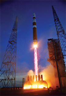
I received a plethora of mail recently either asking or raging about the status of the Boeing IIF, next generation of GPS satellites. I won’t even attempt to recount all the schedules and budgets this critical program has busted. The important point is, according to the latest schedule, sometime this month, hopefully in the next 10 days, IIF-SV1 will arrive at Cape Canaveral in Florida where it will subsequently be integrated with the Delta IV EELV or Evolved Expendable Launch Vehicle. This will be the first EELV to launch a GPS satellite; therefore, the integration and testing times, both on the ground and on orbit, are expected to be considerably more extensive than normal. Plus there are some unique features of the Delta IV that bear watching. The first stage of a Delta IV consists of one or, in the heavy variety, three Common Booster Core(s) (CBC) powered by a Rocketdyne RS-68 engine. Unlike most first-stage legacy rocket engines, which use solid fuel or kerosene, the RS-68 engines burn liquid hydrogen and liquid oxygen. The RS-68 is the first large, liquid-fueled rocket engine designed in the U.S. since the Space Shuttle Main Engine (SSME) in the 1970s, and at more than 63 meters or 206.7 feet in length, the Delta IV (at right) is the tallest rocket in active use.
When you see images of the first GPS IIF launch, the perspective will be a bit different from the venerable Delta II GPS launches of the past.
AEP 5.5C Update
The GPS Wing and 2SOPS (2nd Space Operations Squadron) initiated a software update (see my column in last month’s GPS World) of the ground command and control (C2) system for GPS on January 11, 2010, over a month ago as you read this. To put it mildly, the update did not go as smoothly as planned. There were immediate problems with certain military, commercial, and civilian receivers, plus some other system glitches appeared that are reportedly unrelated. To ensure there aren’t any more unknown receiver problems lurking in the shadows, the GPS Wing issued a unique NANU (Notice Advisory to NAVSTAR Users) through the NAVCEN (U.S. Coast Guard Navigation Center) for civilian and commercial GPS users, and through the GPSOC (GPS Operations Center) for military users, asking for user comments. The GPS is so ubiquitous, and there are so many global receiver manufacturers with so many different GPS receivers on the market today that, not surprisingly, the GPS Wing has been unable to keep track. It is a Herculean task and therefore instead of checking and certifying every GPS receiver manufactured, the GPS Wing issued an updateable ICD or Interface Control Document that all receiver manufacturers use as a voluntary guide to determine compliance. However, even the ICD leaves room for interpretation and is more ambiguous than the GPS Wing intended, so it should come as no surprise that there were and are still receiver issues following the latest AEP update. The GPS Wing is currently receiving more help than they think they need, but this too shall pass; it will just take time. The GPS Wing did not revert to AEP 5.4 (the previous version) because of the upcoming IIF-SV1 launch. The scheduled sequential AEP 5.5C and AEP 5.5D updates are required before the ground control segment can adequately control the more advanced capabilities of the IIF satellites.
The actionable aspect of this update and NANU is that if you are experiencing any problems or glitches with your GPS receiver that occurred after the January 11 update, then you should notify the 2SOPS if it is a military receiver and the NAVCEN if it is a civilian or commercial receiver. The original deadline was January 29, 2010, but I have it on good authority that reports are still being received. So, if you have a GPS receiver issue, please report it.
For civil and commercial users, the U.S. Coast Guard Navigation Center’s address is:
NAVCEN MS7310
7323 Telegraph Road
Alexandria, VA 20598-7310
You can contact NAVCEN by telephone at (703) 313-5900 or go to its comprehensive website.
GPS Civil Focus Day
On February 3 the Commander of HQ Air Force Space Command, General C. Robert Kehler, hosted the 2nd GPS Civil Focus Day. This event was long overdue; the last one occurred more than five years ago. It was one of the best updates I have attended that was specifically crafted for the civilian community. My hat is off to Colonel Dave Buckman and crew for all their hard work that made this event such a success. There were numerous government VIPs present, and it would take several columns to review their input, but suffice it to say the briefings and discussions were candid, informative, and unfortunately not for attribution. Therefore, before I can reveal more I need to be granted permission and that is in the works. Meanwhile we will post the cleared GPS Civil Focus Day briefings on the GPS World website, so watch the GPS World daily news for the location. The important point is that this high-level meeting of the minds underscored that GPS, the global PNT gold standard, is and always has been a dual-use system, and the USAF on behalf of the U.S. government is working hard to meet everyone’s global PNT needs.
Mobile Epiphany and Touch Inspect
To wrap up the column this month, I want to say thanks to everyone who has written me concerning the Touch Inspect software application from Mobile Epiphany I mentioned in my December 2009 GPS World column. The response from the military, civil, and commercial communities has been simply overwhelming, and therefore I am planning an in-depth review of this versatile application in a future issue. I have not historically, as a rule, reviewed software to the same degree that I have hardware, but in this case I am impressed with the application, especially the superb integration of GPS capabilities and the user interface. So a review is in order. Watch this space.
Until next time happy navigating and keep those cards, letters, and e-mails coming.
In the few years I’ve been writing this column, very few subjects have warranted back-to-back newsletter coverage. The new GPS 24+3 onfiguration is one of them. The reason I’ve continued with this discussion is because it will significantly affect your GPS operations, especially if you’re using RTK or DGPS.
What is the new 24+3 GPS configuration?
If you didn’t read my last column, you might want to read it so you have a common frame of reference. Essentially, the effect of the 24+3 configuration will be to increase the visibility of more GPS satellites throughout the day at a given location. In addition to have more satellites in view, you will generally see lower PDOP values which can result in an increase in accuracy; but certainly the increased satellite visibility is the major upside with 24+3.
Remember that the GPS satellites are configured in 6 orbital planes (A, B, C, D, E, F) with X number of satellites in each plane that are referred to as “slots.” For example, slot A1 is the first satellite in the A plane, slot B4 is the fourth satellite in the B plane. Note that the slots aren’t necessarily in numerical order. Following is a graphic presented by the U.S. Air Force in September 2009 to provide an illustration of the planes, and slots within each plane. GLAN is the Geographic Longitude of the Ascending Node.
On the graphic above, note that many of the satellites are paired together. When GPS satellites are paired together, there is little benefit to the user on the ground because the satellites aren’t “spread out”. Ideally, the user on the ground needs the satellites to be “spread out” in the sky which will result in a lower PDOP value (better constellation geometry) and ultimately better accuracy. The satellites are in this configuration today because GPS policy defines a 21+3 configuration. Since there are 30 operational GPS satellites in orbit (six more than required), the six spares are placed near other operational satellites. This isn’t optimal for the user on the ground.
The concept behind the 24+3 configuration is to spread out the satellites more than the current configuration to benefit users on the ground. This involves significantly repositioning three GPS satellites (SVN24, SVN26, SVN49) and slightly repositioning three other GPS satellites (SVN56, SVN46, SVN55).
Following is a tabular listing of each slot in the 21+3 configuration. Please note that the graphic above is a rough graphic for illustration purposes (referencing GLAN) while the tabular data below are the actual values.
Notes:
Epoch: 00:00:00 UTC, 1 July 1993 Greenwich Hour Angle: 18h 36m 14.4s Orbital Slot IDs are Arbitrarily Numbered * Orbital Slots Marked by an Asterisk are Expandable
In the 24+3 configuration, slots B1, D2, F2 are split to B1F/B1A, D2F/D2A, and F2F/F2A. The F designation is Fore and the A designation is Aft.
Following is the tabular data for the expanded slots:
On the B plane, SVN49 is repositioning to slot B1F while SVN56 is moving slightly to slot B1A.
On the D plane, SVN24 is repositioning to slot D2F while SVN46 is moving slightly to slot D2A.
On the F plane, SVN26 is repostioning to slot F2F while SVN55 is moving slightly to slot F2A.
You can refer to the graphic at the beginning of this article to reference the current location (approximate) of each SVN as well as the slot id. The SVN number is to the left of the symbol while the slot id is to the right.
SVN24 has the furthest distance to travel. It began its journey late last month and will arrive in January 2011. SVN49 and SVN26 will both arrive at their destination slots in May 2010.
If they were in a hurry, the satellite travel time could be reduced, but according to folks I’ve spoken to they have to conserve fuel. After the satellite reaches its destination slot, it must have enough fuel to occasionally maneuver as well as retain enough fuel for an end of life boost which could happen many years in the future.
Exactly how many more GPS satellite will my receiver “see”?
I was hoping to publish satellite visibility charts in this column for different regions of the world to illustrate the upside of 24+3. This is where the “rubber meets the road.” I’ve been experimenting with a modified GPS almanac in satellite visibility software to generate these, but I want to confirm the accuracy of the plots before I publish them. I’m close, but not quite there yet.
Also, I want to publish a separate satellite visibility chart for DGPS users. Remember from my last column that SVN49 is a tricky one. It’s still unhealthy since it was launched into orbit last March. Most likely, it will never be usable by SBAS (WAAS, EGNOS, MSAS) and DGPS receivers and will effectively reduce the 24+3 configuration to a 24+2 configuration for those users. Mind you, even if SVN49 is not usable by SBAS and DGPS, the new configuration will still be an improvement over the current configuration.
Look for continuing coverage on the 24+3 configuration. It will be the most relevant GPS topic for day-to-day GPS users in 2010.
Last month, I wrote about the PDA vs. Tablet war. The tablet computer has been around for a long time and struggled to gain widespread acceptance. I also wrote about how 2010 will be a decisive year for the tablet computer.
I guess my timing was right: with the introduction of the Apple iPad last week, 2010 sure has started out with a bang! Admittedly, we’ve known about the iPad for awhile and I even mentioned it in the PDA vs. Tablet column, but didn’t expect the hype to appear for another month or so.
The iPad might turn out to be a technology that transforms the geospatial industry. The iPhone has made inroads into geospatial, but the iPad is another story altogether primarily because it’s not a mutually exclusive proposition. For example, I’m not an iPhone user and won’t be in the foreseeable future. This is not because I dislike the iPhone. On the contrary, I might like to have one. But all my family phones (parents, kids, spouse) are all under my Sprint account. The pain to change is too great.
The iPad is a different story. Its primary function is not a phone. I could see myself purchasing an iPad, especially at $500-600. I’d use it not only as a digital notebook, but also as a mobile GIS device.
Apple iPad announced last week
There will be a lot of debate in the consumer market about which features were included and which features were left out. But, from a geospatial industry technical perspective, I don’t think that matters. It’s got a large color screen (big assumption that it’s outdoor readable), runs 10 hours on a charge, runs third-party applications (albeit not a Microsoft platform) and can interface to a GPS receiver (or use its own). That covers 90 percent of the battle.
The most important indicator to watch is the iPad’s acceptance in the consumer market. Honestly, I can’t figure out if it’s going to be a Newton or an iTouch. Obviously, it’s too early to say. For the iPad to be a success in the geospatial industry, it’s got to reach the success of the iTouch, of which Apple has sold ~31 million units. The geospatial industry will never support the development of a product like the iPad at the $500 price point. There’s just not enough market size to justify it. The geospatial industry needs to ride the wave of consumer market acceptance to benefit from a product like the iPad.
Acceptance of the iPad by the consumer market could produce marked changes in the geospatial industry. The devices would be readily available and might become a default unit for mobile GIS given the low price point and attractive features. It might even be considered a disruptive technology because it would bring an entirely new host of applications and application development tools to the geospatial industry for mobile GIS.
Changing Gears to Geospatial ETL
I want to touch quickly on the subject of geospatial ETL. I have to admit I was a little ignorant about the geospatial ETL (Extract, Transform, Load) industry…and I still am, albeit a little more aware than I was before. The funny thing is that for many years I’ve been dealing with one of the problems that ETL software is designed to solve.
ETL is an acronym for Extract, Transform, Load. These are software tools that facilitate the extraction, transformation, and loading between software systems. Spatial ETL is the same but focused on ETL between geospatial systems.
Wisdom Technologies Fast Reader
I’ve personally run into this problem many times with mapping projects I’ve worked on. I’ve spent countless hours updating maps of the same project that I maintain in both AutoCAD and ArcView/ArcGIS. Yes, I’ve been down the road of importing DWG files into ArcView/ArcGIS and trying to make that work, and I did to some extent, but never to the point that I could abandon one in favor of the other. Granted, if my projects were large enough, I would investigate this further, but generally they aren’t.
Just last month, one of the industry leaders, Safe Software, introduced its FME 2010 product. I spoke briefly with co-founders Don Murray and Dale Lutz about their new product. I’ll be doing more of these sorts of 5- to 10-minute podcast interviews and posting them on the Geospatial Solutions website when the new version goes live in the coming weeks.
Safe Software FME implementation at Washington DOT
In the meantime, click below to listen to my podcast interview with Don and Dale. The interview is about 11 minutes in length. Pay particular attention at the 7:50 minute mark to the discussion about 3D geospatial data.
By Tony Haddrell, Marino Phocas, and Nico Ricquier
We examine the antenna designs that provide GPS functionality to mobile phones and why most phones still do not provide GPS operation indoors. We also see what it will take to make them better.
INNOVATION INSIGHTS by Richard Langley
WHAT ARE THREE THINGS THAT MATTER MOST for a good GPS signal? Antenna, antenna, antenna. The familiar real-estate adage can be rephrased for this purpose, although the original — location, location, location — is valid here, too.
GPS satellite signals are notoriously weak compared to familiar terrestrial signals such as those of broadcast stations or mobile-phone towers. However, if an appropriate antenna has a clear line-of-sight to the satellite, excellent receiver performance is the norm. But what constitutes an appropriate antenna? The GPS signals are right-hand circularly polarized (RHCP) to provide fade-free reception as the satellite’s orientation changes during a pass. A receiving antenna with matching polarization will transfer the most signal power to the receiver. Microstrip patch antennas and quadrifilar helices, two RHCP antennas commonly used for GPS reception, have omnidirectional (in azimuth) gain patterns with typical unamplified boresight gains of a few dB greater than that of an ideal isotropic RHCP antenna.
But what happens when signals are obstructed by trees or buildings or, worse yet, when we move indoors? Received signal strength plummets. A conventional receiver, even with a good antenna, will then have difficulty acquiring and tracking the signals, resulting in missed or even no position fixes. However, thanks in large part to massive parallel correlation, receivers have been developed with 1,000 times more sensitivity than conventional receivers, permitting operation in restricted environments, albeit usually with reduced positioning accuracy. But such operation requires a standard antenna.
So, do the GPS receivers in our mobile phones now work everywhere? Sadly, no. Consumers demand that their phones not only provide voice communications and GPS but also Bluetooth connectivity to headsets, Wi-Fi, and even an FM transmitter, all in a small form factor at reasonable cost. This requires miniaturizing the GPS antenna and possibly integrating it with the other radio services on the platform. Such compromises can, if the designer is not careful, significantly reduce receiver effectiveness with dramatically reduced antenna gain and distorted antenna patterns. This month we look at some antenna designs providing GPS functionality to mobile phones and examine why most phones still do not provide GPS operation indoors or in other challenging environments. We also find out what it will take to make them better.
“Innovation” is a regular column that features discussions about recent advances in GPS technology and its applications as well as the fundamentals of GPS positioning. The column is coordinated by Richard Langley of the Department of Geodesy and Geomatics Engineering at the University of New Brunswick, who welcomes your comments and topic ideas.
GPS is becoming a must-have feature in mobile phones, with major manufacturers launching new designs regularly, and second-tier manufacturers rapidly catching up. A quick test of any early GPS-equipped phone shows that although the incumbent GPS chip (or chipset) has high sensitivity, the integrated end result cannot perform in low signal conditions. Several challenges facing the phone designer are responsible for this, with the main two being the antenna performance and interference in the GPS band generated within the phone platform itself.
Here we explore the antenna’s role in determining overall performance of the GPS function in a mobile phone, and the potential for avoiding some platform jamming signals by choice of antenna technology.We present some results from an ongoing company study, as part of our remit to assist customers at the system integration level in support of GPS chip sales.
Many handset makers are not GPS or even RF experts, and rely on catalog components to provide their GPS and antenna hardware. Often unsuitable antennas are chosen, or the antennas are integrated in such a way that the original operation mode does not work. Study of a number of candidate phones has shown that, due to the small ground plane available, the antenna component may be merely a band-tuning device, with the ground plane contributing the signal collection function.
At the beginning of 2008, our team launched a project to understand and prioritize the problems for handset makers in the antenna area, and to provide better solutions than those currently in use.
The handset designer faces several problems when incorporating a GPS antenna. First, it has to be very low cost (a few cents, probably). Secondly, it has to be broadly omnidirectional, since there is no knowledge of “up” on a mobile phone, although some manufacturers rely on the fact that location will only be needed when the phone is in the user’s hand or an in-car holder. From the GPS receiver point of view, we would like the antenna to be as far from the communications (transmitting) antenna as possible, and also removed from other transmitting services such as Bluetooth, Wi-Fi, and FM. Users must not be able to detune the antenna out of band by placing their hands on the phone, or by raising the phone to their ears. In a perfect world, they would not obscure an antenna either.
Of course, we would also like to remove some of that platform interference at the antenna stage, and techniques such as differential RF inputs (with a differential antenna) have been proposed in the search for better noise-cancellation performance.
All of this leaves the handset designer with an impossible task, since he has run out of space to fit a decent GPS antenna with all the isolation requirements, and we typically measure GPS antennas that average 26 to 215 dB of gain with respect to a reference dipole, which measures around 21 dB compared to an isotropic antenna when integrated in the handset. Given that a 2 dB loss equates to double the time to fix (in low signal environments) or, alternately, double the amount of baseband signal-search hardware in the GPS chip, it follows that we must exert some effort to help handset integrators implement better antennas. In this respect, some larger manufacturers have in-house projects running, but smaller ones do not have antenna design teams and rely on their suppliers to provide solutions.
So, we start with cataloging the requirements, and given that most current implementations are only in the “mediocre to terrible” class, we look at ways of improving things accordingly. Of course, there are good GPS antenna solutions out there, but handset designers have mostly shunned them on the grounds of cost or even size. Restrictions on these parameters severely hamper the antenna designer, as reducing a GPS L1 antenna below its “natural” size — about 4 centimeters for a monopole on commonly used FR4-type printed circuit board (PCB) material — inevitably means either using some higher dielectric material, which adds cost, or folding the structure up, which decreases performance.
Single-ended antennas, such as monopoles and microstrip patches, rely on a ground plane, which in a handset is undersized anyway, and is usually difficult to identify and model. True differential designs (such as a dipole) overcome this problem, but are automatically larger. As handsets get smaller and encompass more “connectivity”
(that is, more radio links, including GPS) and competition for antenna space increases, combined antennas become attractive, as they would at least help with the size issue. However, the isolation problems are increased, and since our various radios all (currently) need individual RF inputs, some new layer of complexity and filtering is needed between antenna and chip.
Theory, Performance. We undertook some practical experiments to get a feel for the gap between an antenna’s theoretical performance and its installed performance when integrated with the other phone functions. At present, the idea of modeling all the radiation interactions and mechanical arrangements within such a platform is beyond the scope of the available tools, and so practical measurements are really our only choice in the quest for better antennas.
Finally, we provide some insight into the future, given the rapid advancements driven by mobile-phone technology and the advent of the low-cost handset for new emerging markets. New challenges loom ahead for GNSS antennas, not the least being more bandwidth and multiple frequencies, and we look briefly at what must be done to keep up with handset manufacturers’ requirements in this regard.
Size of the Problem
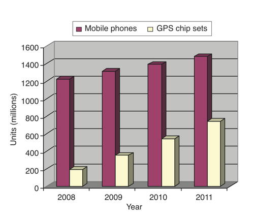
Location-based services in mobile phones is now an expected function by the more discerning user. With more than 500 million users of such services expected by 2011, pressure on manufacturers to provide ever better user experiences and competition between phone manufacturers will bring pressure on the GPS industry for improved performance. GNSS is now the location technology of choice for mobile phones and will remain so provided that the industry can maintain leadership in cost, size, and performance. FIGURE 1 shows the expected penetration of GNSS (mostly just GPS) in the next few years.
Figure 1. GNSS penetration, mobile phones (Image: Tony Haddrell, Marino Phocas, and Nico Ricquier)
With this many users, the market will soon decide whether the performance is up to expectation or not; this in itself will determine GPS penetration going forward.
Vanishing Space. The first challenge facing the RF antenna designer working on a mobile phone is the size of the whole platform. As the size of the average phone continues to fall, manufacturers are understandably reluctant to increase size again to add new features, such as GPS. Consider the wavelengths of a phone’s various RF services. If the corresponding antennas were implemented as dipoles, the antennas would be bigger than the phone. Clearly the competition for antenna space is high. The designer will want to separate the antennas as much as possible to reduce coupling between them, both in the sense of coupling interference from one service to another (known as isolation) and in the sense of spoiling the pattern (or field) of one antenna with another (interaction).
The chip business addresses the space issue through the advent of combination or combo chips, containing such peripheral services as FM (both receive and transmit), Bluetooth, GPS, and Wi-Fi. While helping with space constraints, this development brings new challenges as these radios have to cohabit the same silicon and still perform individually, whatever the other radios are doing (transmitting music to the car radio using FM while navigating with GPS, for example). It follows that combo antennas similarly save space, but since this might involve simultaneous transmit and GPS receive functions, it is very difficult to achieve the necessary isolation, especially if the user’s body can change the coupling between functions.
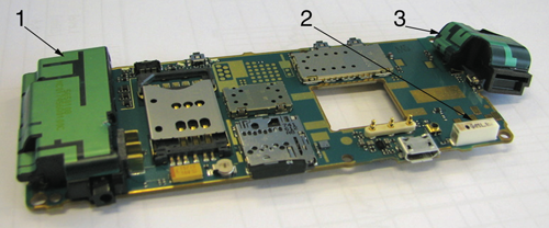
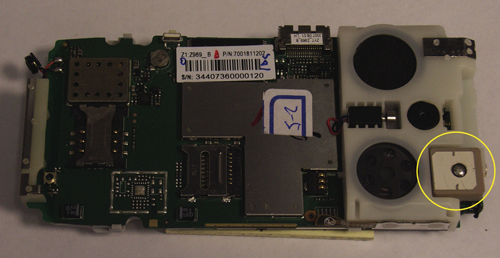
FIGURE 2 shows a modern phone with some antennas identified. Not shown is the FM transmit antenna on the rear (the receive function uses the headset cable). One commercially available combo antenna and two custom-made antennas are designed to fit the mechanical layout of the phone. The GPS antenna has been placed at the top of the phone, relegating the communications antenna (really another combo since it handles four frequency bands) to the bottom of the phone, where it is subject to detuning by the user’s hand. The GPS antenna is of the PIFA (planar inverted F antenna) type, working against the ground plane of the main PCB, and is printed on a plastic molding that also implements a loudspeaker and its electrical connections.
Figure 2. Antennas in a mobile phone: 1. GSM/WCDMA antenna, 2.Wi-Fi/Bluetooth combined ceramic chip antenna, 3. GPS antenna (Image: Tony Haddrell, Marino Phocas, and Nico Ricquier)
Size. Until now, we have not looked at the size of GPS antennas. We know that a dipole (on FR4 PCB material) is about 8 centimeters in length, just a little shorter than the average phone platform. Changing to a monopole halves the natural length, but requires an “infinite” ground plane to work against. Ignoring this requirement, some manufacturers simply print a monopole on the main PCB, and put up with the coupling, losses, and pattern deficiencies that arise. Some while ago, we measured the gain of such an arrangement at about 212 dB relative to the reference dipole. So designers have turned to size-reduced antennas, either by using higher dielectric materials to form them, or by using complex shape and feed derivatives (such as the PIFA in Figure 2.)
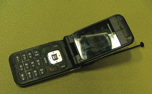
Another combo idea is to use the communications antenna. In the case shown in FIGURE 3, this is a whip-type antenna on a clamshell-type phone. Although the antenna is free for GPS and uses no additional space, the components to tune the whip for GPS and prevent the transmit bands reaching the GPS low noise amplifier (LNA) add both cost and size. So this is not really too attractive, especially when measurements show a 216 dB performance relative to our dipole, along with a poor coverage pattern. In this model, removing the whip and leaving the ferrule to which it connects provided a 6 dB improvement in performance (for GPS only; obviously it spoils the communications function).
Figure 3. Whip antenna combination (Image: Tony Haddrell, Marino Phocas, and Nico Ricquier)
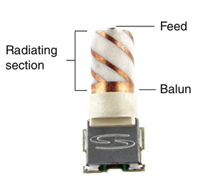
A more conventional approach is to fit an off-the-shelf GPS antenna. The problem here is that any component-type antenna will have been tested with some standardized ground plane, and most are reliant on the ground plane for both tuning, and pattern and gain. A truly balanced design avoids this problem; FIGURE 4 shows an example. Although these antennas have found favor in personal navigation devices for their superior performance, they are not usually considered for mobile phones because of cost and size considerations. This antenna did, however, give us a reference device against which we could make comparative measurements when undertaking the practical test campaign.
Figure 4. Sarantel miniature volute antenna (Image: Tony Haddrell, Marino Phocas, and Nico Ricquier)
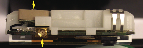
A more usual selection is the patch type, long standard in the GPS industry. One such installation is shown in FIGURES 5 and 6, which offer two views of the same stripped-down phone. The main drawback of this arrangement is the lack of a ground plane visible to the patch antenna, giving both tuning and gain/pattern problems. We measured the gain of this antenna at about 28 dB compared to a dipole antenna connected to the same point in the circuit, which is actually at the better end of the performance range that we see. The designers gave the antenna a position at the top of the phone, as in the Figure 2 phone, but it is still squeezed for space onto the edge of the PCB in favor of the phone’s speakers and the camera components. In this phone, the communications antenna is again at the bottom of the PCB.
Figure 5. Phone with GPS patch antenna at edge of PCB (Image: Tony Haddrell, Marino Phocas, and Nico Ricquier)Figure 6. Edge view of GPS antenna, top of phone removed. This phone includes an external GPS antenna input connector seen here mounted below the patch antenna. (Image: Tony Haddrell, Marino Phocas, and Nico Ricquier)
Interference and Isolation. The related characteristics of interference and isolation are difficult to specify and model, leading to practical measurements as the only way of accurately characterizing them. Of course, since the mechanical arrangement (including plastics, screen, battery, and PCB components) plays such a large part in determining the levels of interference and isolation, these tests can only be carried out once the phone is at the prototype stage, when major surgery to improve any particular aspect is not really an option. This also creates a problem when considering new approaches, as the result may not resemble the stand-alone tests, unless the antenna element chosen really has no significant interaction with the rest of the phone.
Most interference we see in mobile phones gets into the GPS receiver at the antenna. Typically this is followed by an RF filter of some sort, which although it spoils the noise figure, does eliminate the out-of-band transmissions from the other radios on the platform. Usually we see a plethora of self-generated in-band signals that have entered the GPS receiver via the antenna. Although we can’t filter them out, we can reduce the coupling between antenna and source as much as possible. One effect seen in current offerings is that the GPS antenna may actually be much better at coupling to interferers than it is at extracting GPS signals from free space, thus making the problem worse.
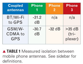
To get a view of the coupling between antennas, we tested a few available phone types to see what was the actual coupling in the antenna band of interest (see TABLE 1). Of course, one advantage of a poor antenna is that its coupling is likely to be less to adjacent antennas. Coupling is also seriously affected by the user holding the phone or the surface on which it is placed. Phones in a pocket seem to be more affected in this way. The table shows measurements with the phone assembled as completely as possible (we have to get connectivity at the antennas) but not being affected by a user or the phone’s environment.
Table: Tony Haddrell, Marino Phocas, and Nico Ricquier
Requirements
To develop requirements for a better antenna implementation, we need to consider the factors discussed above, and to develop numerical specifications against each. Given the variables involving user interaction, mechanical changes from model to model, use cases and the ever-increasing pressure on cost and size, this is far from straightforward. Our team has spent considerable time defining requirements, and a short synopsis is reported here.
In addition to the coexistence requirements (see the next section), the antenna should fulfill the following criteria:
Minimum cost. The antenna should be of low implementation cost, preferably printed and not requiring complex connectivity to the main PCB, or to require any setup and/or tuning in production;
Low loss. The GPS industry is used to antennas delivering around 0–3 dB (isotropic) in an upper hemispheric direction. We believe this will not be attainable in a mobile phone, but we set the gain target at an aggressive -4 dB (isotropic);
Detuning. The antenna must continue to perform to specification with any reasonable detuning environment (such as user handling, pocket, and metal surfaces);
Mechanical arrangement. The antenna should be of minimum dimensions that can fit the phone mechanics. For example, long and thin may be acceptable along one side of the phone. Also placement near the GPS chip avoids lossy RF tracking;
Gain pattern. Essentially omnidirectional, accepting that other parts of the phone may cause localized dips in the pattern.
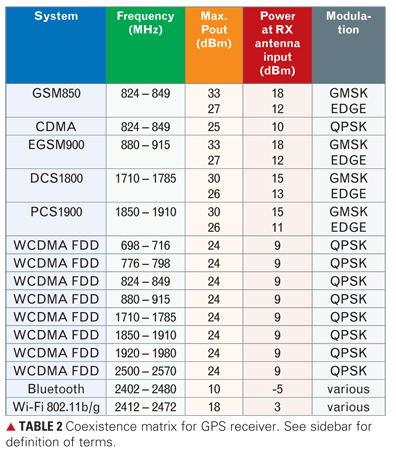
Coexistence and Cohabitation. Initially we aim to define the parameters affecting interaction with other services on the phone platform. By coexistence, we mean the ability to share a platform with the other radios and antennas and only be marginally affected by them, whatever they are doing (such as transmitting full power, low power, or idling, and with any frequency choice). This produces a straightforward immunity table (see TABLE 2) once we have determined the basic isolation between all of the elements. For the purposes of Table 2, we have chosen 15 dB as the minimum isolation value between any two antennas. Obviously there are similar tables for the other functions (GSM, 3G, Wi-Fi, Bluetooth, FM) as well.
Table: Tony Haddrell, Marino Phocas, and Nico Ricquier
A glance at Table 2 will tell the reader that the modern mobile phone implements a vast number of transmit and receive frequencies, modulation types, and standards. Of particular concern to the GPS designer is the advent of wideband CDMA signals, which can cause intermodulation products to appear in band at the intermediate frequency of the GPS receiver. Special receiver techniques are required in this case, but the antenna is unable to help except by being of naturally narrow bandwidth.
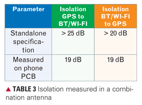
Cohabitation is a newer concept that describes the isolation between functions of the same device. In this respect, we are investigating GPS antennas combined with Wi-Fi and Bluetooth services. This is a fairly natural development, since these functions are all add-ons to a conventional phone platform, and there is a space-saving advantage in the combination. Since Wi-Fi and Bluetooth share the same band at 2.4 GHz, they have arrangements internally that allow them to coexist or choose which service is to be used if a clash is inevitable.
As a precursor to forming some specifications, our team measured a commercially available combined antenna, and TABLE 3 shows the isolation results.
Table: Tony Haddrell, Marino Phocas, and Nico Ricquier
The table highlights the need to measure antennas on a representative PCB, since other coupling factors reduce the specified isolation by >6 dB compared to the manufacturer’s reference setup, where the part is the only component on the demonstration board.
Real-Life Testing
A number of tests were carried out on available solutions to gain some information and experience about current offerings and platforms.
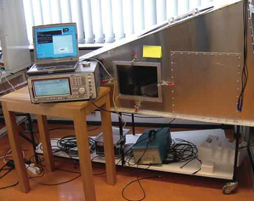
At one of our facilities, we have a GTEM (gigahertz transverse electromagnetic) cell, which was constructed in house and has been verified to be working properly (see FIGURE 7). A GTEM cell is an expanded transmission line within which a uniform electromagnetic field can be generated for determining antenna properties such as gain and bandwidth. The internal space at the septum (40 centimeters) is big enough to handle antenna sizes used by GPS. It has a small side door and some feedthroughs (coaxial) to the bottom plate. The RF foam absorbers used inside the GTEM work well at 1.5 GHz (the cell can work from 100 MHz to above 10 GHz).
Figure 7. The GTEM cell and related test equipment (Photo: Tony Haddrell, Marino Phocas, and Nico Ricquier)
Differential vs. Single-Ended Antennas. The first test conducted concerned comparison of balanced and unbalanced antennas, the theory being that a balanced antenna would help with interference because it would be presented to the GPS receiver as a common mode signal (that is, balanced on the positive and negative inputs). The NXP GNS7560 single-chip GPS solution is configurable for single or differential input to the LNA, and was used to conduct the tests.
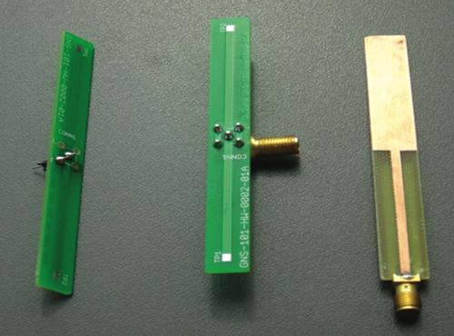
The trial began with calibration of the test setup using the balanced antenna shown in Figure 4, against which we measured a printed dipole antenna and a monopole equivalent, arranged to incorporate a balun to make it of the same size as the dipole (see FIGURE 8). Once this calibration had been made, we sought to generate an interfering signal on the GPS receiver test board so that comparisons of interference rejection could be made. This was done in two different ways, in case the method of exciting the GPS board was subject to resonances or peculiar standing-wave modes. First, we injected an RF interferer into the power supply via the USB cable that was both powering the GPS board and the communications link to it. The jamming created in this manner was increased until a predetermined drop in GPS sensitivity was reached. A number of frequencies were tried and the results compared. In the second setup, we directly applied an RF signal across the ground plane of the GPS board, using a coaxial feed to excite the ground plane, and repeated the stages described above.
Figure 8. Antennas used in the balanced vs. unbalanced antenna testing (Photo: Tony Haddrell, Marino Phocas, and Nico Ricquier)
Results for both tests were within 2 dB of each other, and showed that the differential approach could reduce local jammer pickup by only 4–6 dB. This is probably due to the differential structure being of similar size to the test platform (chosen to be similar to a phone platform), and therefore not achieving true differential coupling to the on-board radiated jammer. With this marginal advantage, we concluded that the benefit was barely justified by the extra complexity and size involved in differential antennas. Note that this conclusion may be different for smaller (for example, high dielectric) differential antennas, although these are currently not available. We are resolved to revisit this possibility at a later date.
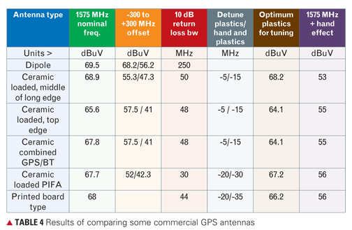
Testing Some Commercial Parts. Having elected to continue in unbalanced-only mode, we tested some commercially available antenna components, which are all aimed at mobile phones and span a range of technologies. Each antenna was tested on its recommended reference design without other mobile phone components or features. However, we did use phone-sized boards, representative plastics, and a real user’s hand in these tests. TABLE 4 shows the comparative results.
Table: Tony Haddrell, Marino Phocas, and Nico Ricquier
For return loss measurements we used a vector network analyzer and a ferrite absorber clamp to suppress cable common-mode effects. For measuring the antenna-received voltage, we used an open-air setup with a horn antenna placed 1 meter away from the DUT (device under test) antenna. The horn is fed with a 100 dBuV 1575 MHz CW signal and the received signal at the DUT is inspected with a spectrum analyzer. The horn is mounted so that we have vertical polarization. Initially, we were only concerned with looking for the maximum attainable voltage and we have positioned the DUT also to vertical polarization. Wooden tables were used to avoid reflections. The last two columns in Table 4 are with plastic in close proximity to the antenna element and the last column is with the plastic grabbed by the hand (as one would grab a phone).
The first thing to note is that of the antennas reported above (which were the best of a bigger number of test pieces) the performance is roughly the same for all of them when configured in their reference mechanical arrangement and not interacting with the phone environment. From the table, we can see that for the particular antenna tested in two positions, its location on the ground plane defines its performance (the ceramic-loaded antenna lost 3 dB in voltage terms when moved to the shorter side of the board). This may be a problem in that the best position performance-wise is not the best for the case where the user interacts with the complete assembly. Also, we see that the user and the plastics have a big effect. In short, the component-type antennas currently available don’t show exciting performance in a real environment, but most are competent GPS antennas when integrated according to their makers’ instructions. However, this is often not possible due to mechanical and other constraints. One drawback of the monopole type of device is its need for a ground-plane-free area underneath the component, and this often conflicts with the requirements of the other antennas, which are looking to maximize the ground plane in the phone.
Novel Approaches, Validation
We started this program to identify the requirements of a good GPS antenna, test some theories and current components, and then develop a new approach. From the foregoing, it is clear that a design that is part of the phone mechanics itself will be better integrated and more predictable in the final implementation. Our design team has begun to model and test some more PCB-centric solutions that attempt to mimic at least the current performance of commercial components, and to minimize the amount of ground-plane loss. We do all our testing on representative (in size and conductivity) phone PCBs. A new approach to thinking about potential arrangements is to use the previously mentioned concept that the whole board is the radiator and the antenna is actually a tuning and feed device. One promising possibility is a slot antenna (or slot feed) formed by removing a small notch of ground plane along the top edge of the phone PCB. Some phones have demonstrated success in forming Bluetooth antennas in this manner, although the lower frequency of GPS does not help.
On a separate path, another idea is to print a PIFA (or similar structure) on the plastics themselves and have it work against the phone ground plane in total. In this case, it is relatively easy to get good performance, but connection of the feed to the main board (where the GPS chipset will be located) is a non-trivial mechanical problem.
Testing of some candidate solutions is under way, and we expect reference designs for customer use to be the deliverable from this work. In addition, it is clear that there is not a one-solution-fits-all conclusion, and that more work will be necessary as phone and GPS designs are further developed.
Acknowledgments
The authors thank the antenna engineering team at NXP’s Mobile and Personal Innovation Center, especially Tony Kerselaers, Felix Elsen, and Norbert Philips who conducted the trials reported here. This article is based on the paper “A New Approach to Cellphone GPS Antennas” presented at ION GNSS 2008.
TONY HADDRELL is a fellow staff architect.
ST-Ericsson in Daventry, England, and a director of iNS Ltd., Weedon, England.
MARINO PHOCAS is an RF systems engineer with ST-Ericsson.
NICO RICQUIER heads the Connectivity Group at NXP Semiconductors in Leuven, Belgium.
Some Mobile Phone Terms
Bluetooth (BT). A communications protocol operating in the 2.4 GHz Industrial, Scientific and Medical (ISM) frequency band, enabling electronic devices to connect and communicate in short-range ad hoc networks.
CDMA. Code division multiple access is a channel access method used by some mobile-phone carriers that allows multiple users to share the same radio frequencies using spread spectrum signals.
DCS1800. Digital Cellular Service version of GSM operating in the 1700 and 1800 MHz bands.
EDGE. Enhanced Data Rates for GSM Evolution, a third-generation (3G) version of GSM.
EGSM900. The Extended GSM 900 MHz band.
FDD. Frequency-division duplexing, a communications protocol that uses different carrier frequencies for transmitt
ing and receiving.
FM. The broadcast frequency modulation band.
GMSK. Gaussian minimum shift keying, a continuous-phase frequency-shift keying modulation scheme used for GSM communications.
GSM. Global System for Mobile communications, the most popular mobile phone standard.
GSM850. A GSM version operating in the 800 MHz band.
PCS1900. Personal Communications Service version of GSM operating in the 1800 and 1900 MHz bands.
QPSK. Quadrature phase-shift keying. A modulation technique used in CDMA systems.
Triplexer. A filtering device to provide isolation between communications and GPS circuits when sharing an antenna.
W-CDMA. Wideband CDMA, an enhanced, 3G version of CDMA.
Wi-Fi 802.11b/g. Wi-Fi describes a standard class of wireless local area network (WLAN) protocols based on the IEEE 802.11 standards operating primarily in the 2.4 GHz band.
FURTHER READING
• Mobile Phone Development
“The Smartphone Revolution” by F. van Diggelen in GPS World, Vol. 20, No. 12, December 2009, pp. 36–40.
• Signal Compatibility Issues
“Jammers – the Enemy Inside!” by M. Phocas, J. Bickerstaff, and T. Haddrell in Proceedings of ION GNSS 2004, the 17th International Technical Meeting of the Satellite Division of The Institute of Navigation, Long Beach, California, September 21–24, 2004, pp. 156–165.
• High Sensitivity GPS Receiver
“A Single Die GPS, with Indoor Sensitivity – the NXP GNS7560” by T. Haddrell, J.P. Bickerstaff, and M. Conta in Proceedings of ION GNSS 2008, the 21st International Technical Meeting of the Satellite Division of The Institute of Navigation, Savannah, Georgia, September 16–19, 2009, pp. 1201–1209.
• Mobile Phone GPS Antennas
“A Compact Broadband Planar Antenna for GPS, DCS-1800, IMT-2000, and WLAN Applications” by R. Li, B. Pan, J. Laskar, M.M. Tentzeris in IEEE Antennas and Wireless Propagation Letters, Vol. 6, 2007, pp. 25–27 (doi:10.1109/LAWP.2006.890754).
“Getting into Pockets and Purses: Antenna Counters Sensitivity Loss in Consumer Devices” by B. Hurte and O. Leisten in GPS World, Vol. 16, No. 11, November 2005, pp. 34–38.
“Miniature Built-in Multiband Antennas for Mobile Handsets” by Y.X. Guo, M.Y.W. Chia, and Z.N. Chen in IEEE Transactions on Antennas and Propagation, Vol. 52, No. 8, August 2004, pp. 1936–1944 (doi: 10.1109/TAP.2004.832375).
“Mobile Handset System Performance Comparison of a Linearly Polarized GPS Internal Antenna with a Circularly Polarized Antenna” by V. Pathak, S. Thornwall, M. Krier, S. Rowson, G. Poilasne, L. Desclos in Proceedings of IEEE Antennas and Propagation Society International Symposium 2003, Columbus, Ohio, June 22-27, 2003, Vol. 3, pp. 666–669 (doi:10.1109/APS.2003.1219935).
Planar Antennas for Wireless Communications by K.L. Wong, published by John Wiley & Sons, New York, 2003.
• Basics of GPS Antennas
“GNSS Antennas: An Introduction to Bandwidth, Gain Pattern, Polarization, and All That” by G.J.K. Moernaut and D. Orban in GPS World, Vol. 20, No. 2, February 2009, pp. 42–48.
“A Primer on GPS Antennas” by R.B. Langley in GPS World, Vol. 9, No. 7, July 1998, pp. 50–54.
By Ruizhi Chen, Heidi Kuusniemi, Yuwei Chen, Ling Pei, Wei Chen, Jingbin Liu, Helena Leppäkoski, Jarmo Takala
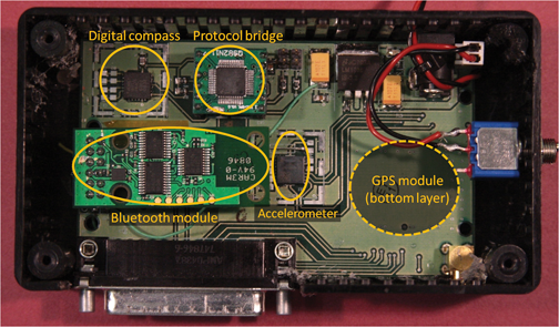
Currently, no single technology, system, or sensor can provide a positioning solution any time, anywhere. The key is to utilize multiple technologies. We are now exploring a multi-sensor multi-network (MSMN) approach for a seamless indoor-outdoor solution. Its hardware platform is described in the previous article. The digital signal processor (DSP) is embedded in the GPS module. All sensors are integrated to the DSP that hosts core software for real-time sensor data acquisition and real-time processing to estimate user location. A smartphone handset provides wireless network measurements.
Positioning Algorithms
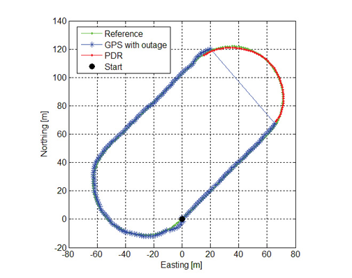
The multi-sensor positioning platform enables a positioning solution with a combination of GPS and reduced inertial navigation system (INS), or GPS and pedestrian dead reckoning (PDR). The reduced INS consists of a 3D accelerometer and a 2D digital compass, as a low-cost alternative to augment GNSS positioning. The reduced INS combined with GPS uses a loosely coupled Kalman filter for data integration, while the combination of PDR and GPS uses algorithms for estimating the position change with pedestrian step-length estimation.
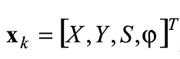
PDR. The PDR solution uses human physiological characteristics, implemented in a local-level frame, with equations:
where k denotes the current epoch, Y is the coordinate in East direction, X is the coordinate in North direction, S is step length, and φ is the heading.
The PDR positioning algorithm includes step detection, step length estimation, determination of heading, and positioning.
To achieve an accurate heading, compass measurements are corrected with an empirical online estimated error model, which requires some training data.
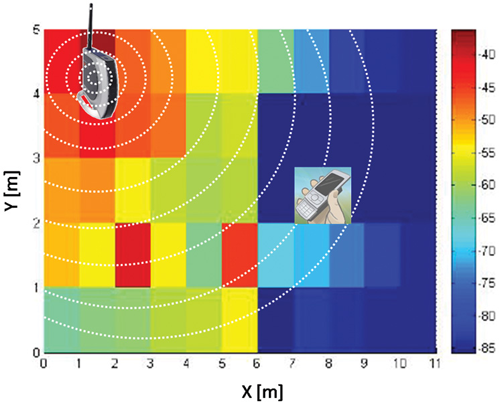
WLAN and Bluetooth. Figure 1 describes the basic concept of the WLAN or Bluetooth locating solution using a fingerprint database approach. The circles around the access point (AP) in the figure represent the radio coverage area and the color the signal strength. This radio map is a simplified example representing measurements from just one AP.
FIGURE 1. Sample WLAN or Bluetooth fingerprint map, in meters.
For the fingerprinting approach, the received signal strength indicators (RSSIs) are the basic observables. The whole process consists of a training phase and a positioning phase. During the training phase, a radio map of probability distribution of the received signal strength is constructed for the targeted area. The targeted area is divided into a matrix of grids, and the central point of each grid is referred to as a reference point. The probability distribution of the received signal strength at each reference point is represented by a Weibull function, and the parameters of the Weibull function are estimated with the limited number of training observation samples. Based on the constructed radio map, the positioning phase determines the current location using the measured RSSI observations in real time.
Given the observation vector , the problem is to find the most probable location (l) with the maximized conditional probability , maximized by Bayesian theorem as:
We applied an assumption of Hidden Markov Models (HMM) to represent the pedestrian movement process. The locating problem is then translated into finding such a state sequence (locations) that is most likely to have generated the output sequence (the measured RSSIs) assuming the given HMM model. The Viterbi algorithm typically solves these kinds of problems efficiently. This study also utilizes the Viterbi algorithm to trace the user trajectory.
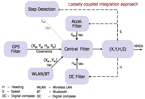
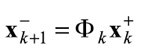
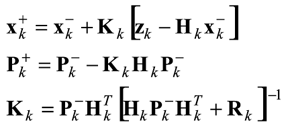
MSMN. The general integration scheme combining the GPS output, sensor measurements, WLAN, or Bluetooth output, and their variance estimates is depicted in Figure 2. A simplified representation of the central filter combining different input sources can be described with typical Kalman filter equations. The measurement model is zk= Hkxk+vk where the state estimate vector is ,
with X, Y, and φ as previously defined, and S the user horizontal velocity (speed). The measurement vector is given as
where g refers to GPS, W to WLAN/Bluetooth, acc to accelerometer, and dc to digital compass. The matrix Hk is the design matrix of the system and the vector vk is the measurement error vector.
FIGURE 2. Integration scheme for multi-sensor, multi-network positioning approach
The recursive sequence includes prediction and update steps. The prediction step includes the typical equations of
and
while the update step includes
Indoor Test Results
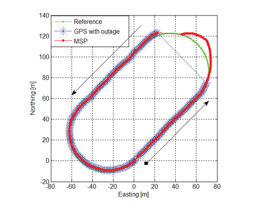
A field test has been carried out on a sports field, described in the accompanying article (see Going 3D). An indoor test was carried out in an office-building corridor, but the test started and ended in an outdoor terrace area. During the test, the indoor corridor was covered with eight WLAN and three BT APs.
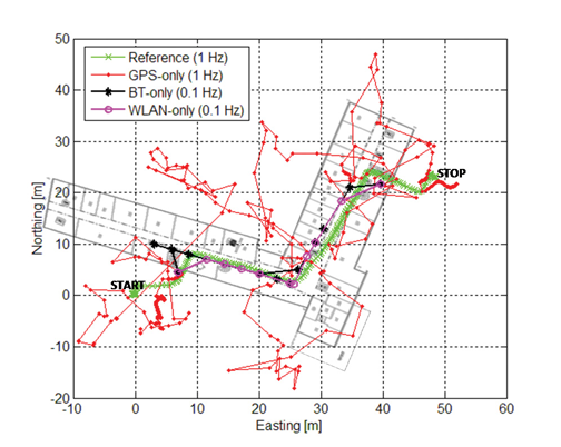
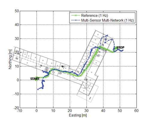
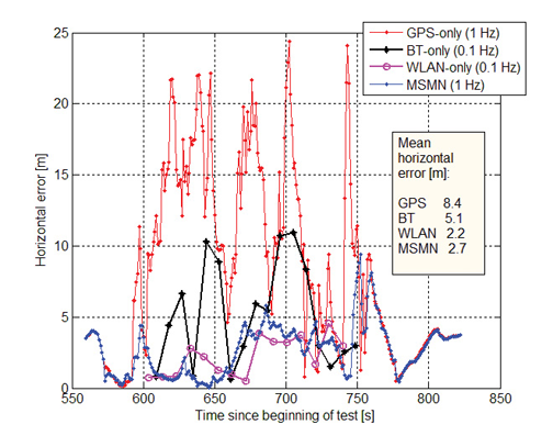
Figure 3 shows the positioning results of the GPS-only (red), Bluetooth-only (black), and WLAN-only (magenta) solutions; Figure 4 shows that of the integrated multi-sensor multi-network (MSMN) solution (blue) for an outdoor-indoor-outdoor test. A reference trajectory is in green in both figures and building outlines in grey. The position update rate achievable by the WLAN and Bluetooth fingerprinting approach is only 0.1 Hz whereas the GPS-only and the integrated MSMN solutions are obtained every second and thus have a higher availability.
FIGURE 3. Pedestrian test results with GPS-only, BT-only, and WLAN-only positioning approaches with respect to a reference trajectoryFIGURE 4. Pedestrian test result with the multi-sensor multi-network positioning approach with respect to a reference trajectory
Figure 5 shows the horizontal errors obtained with the different positioning solutions over time in the indoor test. A mean horizontal error of 2.2 meters was achieved with the WLAN solution. The Bluetooth solution is not as accurate as the WLAN solution, due to the smaller amount of BT APs; it achieved a mean horizontal error of 5.1 meters. When moving inside the corridor, the GPS solutions are used for the MSMN integration only with very low weights due to their poor quality. GPS is mainly used as a source of location outdoors where the test starts and ends. The mean horizontal error of the GPS-only solutions during the whole test is 8.4 meters. WLAN- and Bluetooth-derived locations and the self-contained sensors are the main sources used inside the building for the MSMN positioning solution: the mean horizontal accuracy o
btained with MSMN is 2.7 meters with a solution availability of 1 Hz.
FIGURE 5. Horizontal errors of GPS-only, BT-only, WLAN-only and the MSMN positioning approaches with respect to time in the pedestrian indoor test
The MSMN solution obviously performs much better than a GPS-only solution indoors. The track of the pedestrian walking inside the corridor can be identified clearly, which is not the case with typical approaches of GPS-only or GPS/low-cost sensors. WLAN fingerprinting provides good position accuracy indoors, but the MSMN solution provides the best result when taking into account positioning accuracy and the solution availabilities in both time and space domains.
Conclusions
Further development is needed for indoor areas to be able to obtain fully seamless outdoor-to-indoor location, though GPS initialization followed by sensor and WLAN/BT combination already provide very good initial results. Additional sensors and more refined pedestrian-specific algorithms will be added to further improve the positioning accuracy.
To enrich user experience of location-based services and personal navigation, three-dimensional models such as those used in urban planning are added to a smartphone platform, without the requirement of additional hardware.
Most current map applications for smartphones and other devices providing location-based services (LBS) are based on two-dimensional maps. Three-dimensional (3D) city models are widely used in applications such as engineering design, environmental modeling, and urban planning. Adapting such models for use in smartphones would make it possible to render 3D scenes in real time, enriching contents and user experience for personal navigation and LBS. A delimited yet large-scale event such as the upcoming 2010 World Exposition in Shanghai provides a promising area for system development and testing.
3D visualization consumes a large amount of computing power, and most of the current successful applications run in a PC environment, as does the Google Earth 3D application. It is still a very challenging task to implement 3D visualization in an embedded system such as a smartphone.
This article presents an entire 3D personal navigation system based on a smartphone platform, the Nokia S60 platform. The study covers the following aspects:
3D personal navigation and LBS service in a smartphone
3D city modelling, and
multi-sensor positioning.
The objectives of the work include prototyping an entire handset-based 3D personal navigation and LBS system utilizing WLAN/Bluetooth positioning technologies, handset built-in GPS/AGPS, and 3D modeling and visualization (basic demonstration scenario), as well as presenting a multi-sensor positioning (MSP) platform in addition to the handset software (advanced demonstration scenario).
3D Personal Navigation and LBS
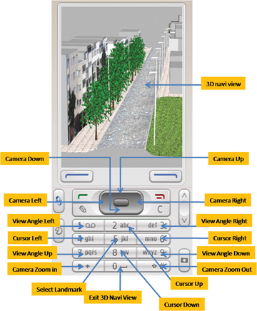
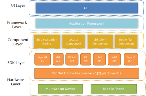
No additional hardware is added to the Nokia Series 60 (S60) smartphone platform to achieve the 3D visualizations or other functions in the software. Figure 1 demonstrates the functionalities and features available in the 3D viewing of the LBS software. Figure 2 shows the general architecture of the software.
FIGURE 1. Functionalities of the 3D LBS softwareFIGURE 2. General architecture of the 3D personal navigation and LBS software
The software development work focuses on the UI layer, framework layer, and component layer. The software mainly includes the following components:
the 3D visualization engine based on OpenGL ES,
the route plan component,
the locator component,
the LBS client component, and
UI and framework.
Most of the challenging tasks are included in the development of the elements in the component layer, especially in the development of the 3D visualization engine based on the OpenGL ES API that is available from the S60 platform SDK (Software Development Kit). The high-level 3D visualization engine architecture covers the interface layer, the core engine layer, and the data management layer. The first one is responsible for cross-component functional communication, request handling, and data exchange. It provides users with the 3D scene visualization functionalities to access the core engine layer via a single class called NaviSceneControl, which includes all the operations of the 3D visualization: scene zooming, view angle rotating, scene and cursor moving, and selecting route planning and virtual navigation.
The core engine layer takes care of the 3D scene visualization computation and model object management. To enable the 3D visualization for a large region, the objects in the scene are classified into two categories in this layer. One is the 3D models like buildings, trees and poles, while the other is texture of land surface, which consist of ortho-rectified digital aerial photos. All the objects are processed as tiles according to the incoming parameters from the interface layer. Therefore only a small subset is loaded dynamically instead of the whole data.
The data management layer accesses the 3D models and ground-texture images persistent on the flash disk of the mobile phone through an independent thread. To reduce the data size of the 3D models, the original .3ds file created from 3D Max Studio software is compressed to fulfill the requirements of the mobile device.
A simple route plan component is implemented in the software to enable to the user to find and view the route to his or her destination. In order to be able to show the entire route, the calculated route will be displayed on top of a 3D view with a downward camera at a high altitude. The 3D scene in this case looks like an orthoimage. An orthoimage shows objects in the perpendicular view to the projection plane of the objects.
The locator component aggregates the positioning information either from the built-in positioning sensors in the smartphone, a GPS receiver, and a WLAN (Wireless Local Area Network) or a Bluetooth chip, or any external positioning device, such as also the multi-sensor positioning (MSP) device developed in this project. It forwards the positioning information including the location and heading information to the route plan component and the 3D visualization engine to accomplish the navigation functions.
The purpose of the LBS client component in the handset software is to access the LBS server.
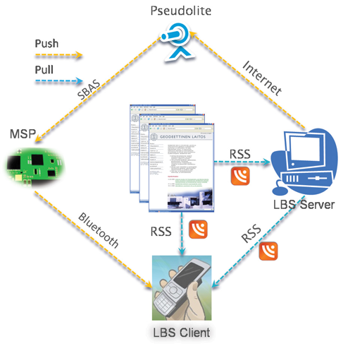
Figure 3 shows the overview of the mechanism for delivering the location-based services. The services are classified into two categories: the static services and the dynamic services. The static services include those services that are not changing in time. For example, POIs (points of interest) belong to this category of service. The static services are stored in a database that can be downloaded from the Internet by the users in advance. The users can store the database in the memory card of the phone before running the 3D personal navigation and LBS software. With this approach, it saves the data transmission fee for the end-users when accessing the LBS. The dynamic services cover those services that change in time. For example, a piece of real-time news is one of the typical dynamic LBS. For accessing the dynamic LBS, the Really Simple Syndication (RSS) technology is adapted in our implementation.
FIGURE 3. Mechanism for delivering location-based services and information
The LBS client component is implemented so that the handset will pull automatically the news in the background in real time via a widget reader embedded in the LBS client component. Whenever new information is uploaded to the LBS server or to the registered web pages, mobile users will be notified.
In addition to RSS technology, another approach to broadcast LBS information is considered in the system: to disseminate the LBS information via an SBAS (satellite-based augmentation system) pseudolite. The dynamic LBS information (e.g., a short message) can be first encoded into a user-defined SBAS message. The message encoded is then sent to a pseudolite from which the message is broadcast. The corresponding SBAS message can, in fact, be received by any SBAS-enabled receiver located within radio coverage area of the pseudolite. However, the encoded LBS message can be decoded only with the receiver that has a special firmware, developed in this case by the Finnish Geodetic Institute (FGI). Having received and decoded the LBS messages transmitted from the pseudolite with a dedicated receiver, for example the MSP device part of the more advanced demonstration scenario of the project, the content of the message is then encoded to a user-defined NMEA (National Marine Electronics Association) message and transmitted to a mobile phone in the vicinity via a Bluetooth connection as shown in Figure 3. This solution of LBS data distribution is available only to a very limited number of users with receivers carting a special firmware developed by FGI.
3D City Modeling
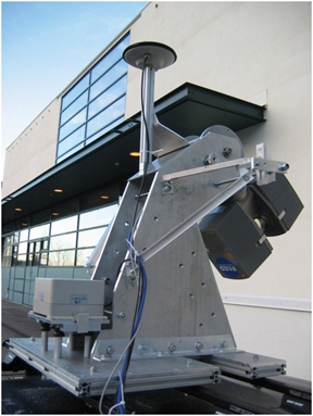
Due to the memory limitations of a mobile phone, there are certain requirements for the 3D models applied. In our study, a test scene for model reconstruction is focused on a street in Espoo, Finland, in an ordinary residential area. A vehicle-borne mobile mapping system ROAMER (see photo) developed by FGI performed the data acquisition. It consists of a carrying platform, a positioning and navigation system, and a 3D laser scanner system. With the ROAMER system, visible objects can be measured with an accuracy of a few decimeters with a maximum vehicle speed of 50–60 km/hour, and the data for the desired objects can be collected within the range of several tens of meters.
ROAMER vehicle-based mobile mapping system.
A large amount of data is produced from the system, and noise and outlier points are needed to be removed. Valid data is classified into different point groups using an automatic algorithm developed by FGI. These point groups include buildings, trees, roads, and poles. Models are then reconstructed based on these classified point groups.
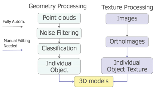
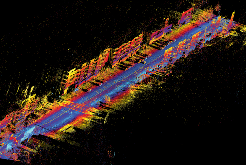
Modeling methods are developed to meet the application requirements of personal navigation: small model size, high accuracy, and good visual appearance. Small model size is achieved by simplified object geometry and reduced texture resolution. Model accuracy is controled by extracting building outlines from a classified point cloud and overlapping with the final 3D model. The model completeness is checked by comparing the resulting model with original images. Good visual effect is realized by applying photo-realistic texture. Photo-realistic texture provides rich information for the 3D scene reconstructed. Figure 4 presents the total process of the 3D modeling, in which only the individual object texture and the final model constructions require manual editing. Figure 5 shows the raw data retrieved and Figure 6 presents the final 3D models of the test area.
FIGURE 4. The process of 3D modelingFIGURE 5. Raw data retrieved from the test area with FGI’s ROAMER systemFIGURE 6. Reconstructed 3D scene of the test area
To import the final 3D models to a mobile phone, the size of an individual model is restricted to less than 100 kb. To optimize model size, a row of buildings is divided into several building blocks.
Multi-Sensor Positioning
As long as open-sky satellite-signal conditions are available, there are no problems to locate a mobile user with the built-in GPS receiver of a smartphone with a positioning accuracy of a few meters. However, most popular location-based services occur in GNSS-degraded environments such as in indoor environments and urban canyons. Locating a mobile user seamlessly any time anywhere under any circumstance is still a very challenging task, especially to implement such an indoor/outdoor positioning solution in a digital signal processor (DSP) platform.
FGI is now developing a DSP-based multi-sensor positioning platform to approach a seamless indoor/outdoor locating solution. The platform consists of a GPS module, a 3D accelerometer, and a 2D digital compass (Figure 7). A DSP is embedded in the GPS module. All sensors are integrated to the DSP that hosts a core software for real-time sensor data acquisition and real-time processing to estimate user’s location.
FIGURE 7. Hardware platform
The multi-sensor platform provides opportunities to investigate the positioning solutions with a GPS/Reduced-INS (Inertial Navigation System) combination or GPS/PDR (Pedestrian Dead Reckoning) combination. The Reduced-INS combination is defined as a combination of a 3D accelerometer and a 2D digital compass, and is a very low-cost approach of sensor augmentation. The GPS/Reduced-INS implementation is implemented in a loosely coupled Kalman filter, while the GPS/PDR algorithm is based on pedestrian-targeted dead reckoning, with heading error and step length estimation methodology.
Preliminary tests analyzing both GPS/Reduced-INS and GPS/PDR solutions have been carried out in a sports field on a 400-meter running track. In order to simulate a GPS outage situation, the GPS measurements were ignored for one minute. During this one minute “outage,” the traveling trajectories are estimated with the Reduced-INS solution and the PDR solution. Figure 8 shows the trajectory of the Reduced-INS solution, while Figure 9 shows that of the PDR solution.
FIGURE 8. Trajectory estimation for the 1-minute GPS outage using Reduced-INS approachFIGURE 9. Trajectory estimation for the 1-minute GPS outage using the PDR approach
The Reduced-INS approach provides a reasonable result with a positioning accuracy of about 20 meters at the end of the forced 1-minute GPS outage. The PDR approach provides a better prediction in this case, resulting in only a couple of meters of error after the 1-minute outage of absolute location input from the GPS, because the heading errors are modeled carefully utilizing previous training with data from a previous run along the same track as well as accurate step detection estimation.
Conclusions
The prototype system will be tested and demonstrated at the 2010 World Expo in Shanghai, implemented with a smartphone software package: anyone with a Nokia phone (S60 with built-in GPS and WLAN/BT) can experience the 3D personal navigation and LBS service in the Expo area by downloading and installing the 3D models. The prototype has so far met these challenges: the high performance required of real-time 3D visualization in a smartphone; high positioning availability with acceptable accuracy in indoor and outdoor environments; and the demanding requirements of the 3D models for a small phone, including small model size, high accuracy, and good visual appearance.
Manufacturers
The multi-sensor positioning platform consists of a Fastrax iTrax03 GPS module, a VTI SCA3000-D1 3D accelerometer, and a Honeywell HMC6352 2D digital compass. The ROAMER mobile mapping system consists of a Faro LS 880HE80 terrestrial laser scanner, two AVT Oscar F-810C cameras, and a NovAtel SPAN geo-reference system.
RUIZHI CHEN is a professor and head of the Department of Navigation and Positioning at the Finnish Geodetic Institute, where Heidi Kuusniemi is a specialist research scientist, Juha Hyyppä is a professor and head of the Department of Remote Sensing and Photogrammetry, Risto Kuittinen is director general, Yuwei Chen is a specialist research scientist, and Ling Pei, Lingli Zhu and Jingbin Liu are senior research scientists.
JIXIAN ZHANG is a professor and president of the Chinese Academy of Surveying and Mapping, where Yan Qin and Zhengjun Liu also work as the director of the Department of Research and Development and the group leader in the Institute of Photogrammetry and Remote Sensing, respectively.
JARMO TAKALA is a professor and head of the Department of Computer Systems at Tampere University of Technology in Finland, where Helena Leppäkoski is a researcher.
JIANYU WANG is a professor at the Shanghai Institute of Technical Physics, Chinese Academy of Sciences.
The U.S. Air Force GPS Wing and 50th Space Wing have begun repositioning GPS satellites in space to fly what they call the 24+3 or Expandable 24 constellation plan. The initiative will take up to 24 months to fully implement. Benefits to users will be slowly realized during that time, as the number of GPS satellites in view will increase, potentially increasing GPS receiver accuracy.
The plan significantly alters the current configuration of 30 GPS satellites on orbit. Several newer satellites now fly in tandem, side by side, with older satellites, as a hedge against their eventual failure. This policy has effectively limited constellation geometry to that of 24 satellites.
The policy change was driven at least in part by the desire to improve satellite visibility for U.S. and allied military operations in Afghanistan and Iraq, where mountainous terrain can hamper signal coverage for troops on the ground.
The first GPS space vehicle (SV) to move, SVN24, began its long journey on January 13. This satellite has the farthest to travel, and will not reach in its new slot for approximately 12 months (January 2011). The two others, SVN49 and SVN26, will affect the geometry much sooner. SVN49 started its four-month journey on January 21, destined to reach its new home in May 2010. SVN26 will stir on February 8 and should also find itself in its new slot by that time, if all goes as planned.
SVN24 will take a full 12 months because the operators must have maneuvering fuel onboard when it reaches its final orbit location for station keeping and Delta-V maneuvers; and they must conserve fuel for end-of-life in as much as 15 years to boost the satellite into a safe retired orbit.
Civil Benefits. 24+3 will especially benefit surveyors and other professionals using real-time kinematic (RTK) positioning. These users currently require six satellites in view for a very precise (centimeter accuracy) position.
In the last few years, some users that require long dwell times and experience high mask angles have been forced to use GLONASS satellites as an augmentation, which works, although GLONASS satellites have historically been less accurate than the GPS. When 24+3 is fully implemented, GLONASS augmentation may no longer be necessary for these users.
New Ground Software. The GPS Wing also trumpeted the advent of improved capabilities through a new ground-system software release. These include telemetry, tracking, and commanding for the new GPS IIF space vehicle — as yet unlaunched. On-orbit capabilities planned to arrive with the IIF Block span the new L5 navigation signal for civil users, continued and more robust security-wise deployment of the encrypted military-only code known as M-Code, on-orbit crosslink (between GPS satellites) improvements, and overall signal power increases.
In November and December 2009, the new software uploaded operational GPS IIA and IIR space vehicles with navigation data and completed normal operational functions.
Penny-Wise, Pound-Foolish U.S. Coast Guard to Pull Loran Plug
The U.S. Coast Guard announced on January 7 that the it will cease broadcasting the North American Loran-C signal on February 8.
“As a result of technological advancements during the last 20 years and the emergence of the U.S. Global Positioning System, Loran-C is no longer required by the armed forces, the transportation sector, or the nation’s security interests.”
The force, and President Barack Obama’s fiscal year 2010 budget which it cited, go against the unanimous recommendation of the Independent Assessment Team, empanelled by a previous administration and led by Bradford Parkinson, founding program director for GPS: “complete the eLoran upgrade and commit to eLoran as the national backup to GPS for 20 years.” To pay for expert advice and then ignore it is a time-honored tradition of U.S. government.
Senator Susan Collins, ranking member of the Senate Homeland Security and Governmental Affairs Committee, called the Coast Guard plan a “mistaken decision,” adding that “A lone system is problematic and ill-advised on so many levels. We need Loran as a backup to GPS.
“Pulling the plug on Loran now will likely prove penny-wise and pound foolish, because there is no other system, or constellation of systems, that offers a more robust and cost-effective backup to GPS than eLoran. It is my urgent request that the Secretary reconsider this ill-informed decision.”
Galileo Satellites Awarded to OHB
The European Commission awarded on January 7 contracts for deployment of Galileo’s initial operational capability in space. The first order of 14 satellites goes to OHB System AG of Bremen, Germany (as indicated, but not confirmed, in these pages last month).
The EC bestowed a contract for system support services upon ThalesAleniaSpace of Italy, and one for launch services to Arianespace of France. Initial deployment and service provision of Europe’s satellite navigation system is now envisioned for early 2014.
Procurement contracts for ground mission infrastructure, ground control infrastructure, and operations should be awarded by mid-2010.
The OHB order carries a value of €566 million (U.S. $811 million), with delivery of the first satellite in July 2012. One satellite is expected every 1.5 months thereafter, with the last one scheduled to be delivered in March 2014.
Compass at Three
China launched a third Beidou-2 or Compass navigation satellite on January 17, destined for geostationary (GEO) orbit. A previous middle-Earth orbit (MEO) craft went up in April 2007 and a GEO in April 2009. By January, that GEO had drifted about 16 degrees from its initial slot, possibly indicating it is uncontrollable although some reports indicate the satellite is still usable.
Eventually, China plans five GEOs and 30 MEOs. The initial Compass system will provide the Asia-Pacific region with navigation, timing, and short-message communication services as early as 2015, with a plan for global coverage by 2020.
Compass will offer an open service (free positioning and timing services, positioning accuracy 10 meters, timing 10 nanoseconds), and an authorized service, with “more secure” position, velocity, timing, and communications data as well as a higher level of integrity.
The government also unveiled an official, Chinese-language-only Compass website, www.beidou.gov.cn.
Deterministic risk modeling, the basis of the Efficient Market Hypothesis (EMH) at the core of modern quantitative finance, is known to be fundamentally flawed, but its elegance and convenience has blinded researchers to growing evidence of its weaknesses. The near-complete acceptance of the EMH led to models that dramatically accentuate its flaws, which in turn led to absurd but eagerly accepted conclusions for loan-default risk. These models proved dramatically vulnerable to changes in the housing market in 2007–2008 and led directly to the ensuing crash.
The gross inattention to potential anomalies and violations of nominal behavior that characterize quantitative finance fortunately do not apply to satellite navigation integrity assurance. Similar techniques and probability distributions are used, but understanding what can go wrong leads to detailed emphasis on modeling and mitigating rare events. Where significant uncertainty exists, conservative assumptions try to be robust to it. Thus, certification of satellite- and ground-based augmentation systems (SBAS and GBAS) likely demonstrates that these systems meet their integrity risk requirements with substantial margin.
Despite this, the predominant use of deterministic models for risk assessment is dangerous because it purports to provide guaranteed bounds on uncertainty that do not apply in practice. The conservative nature of satellite navigation risk assessment greatly reduces but cannot eliminate the underlying integrity risk, while it leads to performance losses with potentially unmeasured safety impacts. Given the uncertainty that is present, probabilistic models are much better suited to providing “illusion-free” risk assessments that enable realistic system-level design trade-offs.
Economics. Decades of financial theory are based upon the assumption that the normal (Gaussian) distribution applies to financial markets. In spite of common-sense arguments to the contrary, assuming that it does is too convenient to give up, and the theories it gives rise to are so useful that it was thought better to force-fit the model to financial processes. Academic and professional preference for tractable, analytical, easy-to-use models trumped the search for truth.
The simplification of correlation into a single parameter made it easier to fit historical data on mortgage default risk correlation to a tractable model. Despite this, the relative rarity of defaults prior to 2000 made any correlation model based on historical default data highly uncertain. An EMH-based market-driven model for default risk correlation became instantly popular, enabling the creation of complicated mortgage-backed derivatives without in-depth analysis.
The simplicity of the Value-at-Risk output that encouraged its widespread use in corporte risk assessment allowed managers to forget that it was only useful to, at most, the 99th percentile. It quickly became thought of as an actual worst-case bound on losses and treated as such in portfolio optimization. Loss reserves throughout the economy fell far short of what was needed. In retrospect, such approaches that oversimplify risk to the point where managers think they fully understand it are worse than useless, as they are so likely to be abused. Experts should understand risk in all its complexity and communicate that risk to decision-makers as fully as possible.
Mathematics. This financial experience suggests that, as Albert Einstein said, “As long as the laws of mathematics refer to reality, they are not certain; and as far as they are certain, they do not refer to reality.”
Deterministic models provide precise quantification of uncertainty whose accuracy and precision are illusory because they depend wholly on the assumptions used to generate the results. Probabilistic models also produce imprecise outputs, but the imprecision is real, and the goal of these models is to identify this lack of precision, rather than cover it up.
Because the probabilistic approach is so philosophically different from the deterministic one, it is likely that more traditional deterministic risk models will remain dominant. These require multiple assumptions regarding uncertain behavior and simplifications to make the resulting model tractable and useful for analysis. Danger lies in forgetting how these models were created and growing to believe in them too strongly while ignoring all contrary data, as happened with the EMH.
To avoid this, assumptions and simplifications on which deterministic risk models are based should be highlighted not only during the modeling process but also when results are presented. If these shaky foundations are consistently emphasized, fewer people will be tempted to willfully or accidentally misinterpret the results, and researchers will be less likely to extrapolate from one flawed model to another.
Lessons for SatNav Integrity
We must first recognize that integrity or safety assurance for satellite navigation is a unique application of risk assessment in which the aim is to protect passengers from the consequences of very rare but potentially hazardous threats. As in the financial world, the Gaussian probability distribution is used extensively to model nominal error behavior and to compute position-domain protection levels intended to bound worst-case user position errors at the integrity-risk probabilities required for user safety. The Gaussian model is a convenient, efficient means to communicate ground-system errors to SBAS and GBAS users in a single parameter: the standard deviation (or sigma) of range-domain errors.
Great care is taken in using the tails of the Gaussian assumption to bound rare-event errors under nominal conditions (so-called rare-normal errors). Extensive studies of GPS, SBAS, and GBAS data show that, while the Gaussian distribution approximately holds in many cases and is usually a good model within the 99th percentile of errors, it is not a good description of rare-event behavior. In particular, rare-event tails of actual data often considerably exceed what is predicted by the Gaussian distribution. Several reasons exist, but the dominant one is the phenomenon of mixing of errors with different underlying actual distributions. This makes sense: rare-normal errors are not really normal but are instead combinations of off-nominal conditions that have different causes.
Because use of the Gaussian distribution is built into the SBAS and GBAS standards, the primary defense against its inapplicability at low probabilities is to inflate the sigmas broadcast by SBAS or GBAS (or assumed in user equipment) such that the assumed distribution overbounds the actual, unknown (and likely very complex) error distribution at the probabilities that matter for user safety. This is a difficult problem. No matter what approach to deriving bounding inflation factors from collected data is used, no means of proving rare-event error bounding by Gaussian distributions exists or can exist, given that the required assumptions cannot be proven. Despite this, conservatism and common sense in deriving inflation factors (and then applying additional margin for “unknown unknowns”) should sufficiently cover the underlying uncertainty.
Even after inflation has been applied, reliance on Gaussian error models becomes much more critical when they are extrapolated to derive distributions for squares of errors, as is done in receiver autonomous integrity monitoring (RAIM) and in real-time monitoring of the broadcast sigma parameters. Errors in the Gaussian error model are greatly magnified when squared and then assumed to follow a chi-square distribution.
History. Using GPS performance to build models of failure probabilities and anomaly behaviors suffers from a lack of data since GPS was not fully commissioned until 1995. Estimating the prior probability of sudden, unpredictable failures in GPS satellites is mostly based upon the observed failure history of GPS satellites in orbit — but such failures are quite rare and are not consistent across all satellites. They occur more frequently as satellites approach end-of-life, and they change as different satellite blocks deploy over time. There is no guarantee that future satellite or Operational Control Segment performance will correspond to that observed in the past. It is risky to estimate one failure rate across all satellites.
For SBAS and GBAS, conservatism and common sense must again be applied to limit the impact of these uncertainties. Failure-rate estimates are made from data where different satellites are combined, but significant margin is applied to account for differences among satellites. The resulting prior probabilities for failures are conservative for all fault types and extremely conservative for faults where limited or no data exists. The problems of relying on limited historical data are even more severe when threat models are created to represent possible system behaviors when a particular fault or anomaly (for example, satellite signal deformation, ionospheric storms) occurs. In the case of satellite signal deformation, deterministic threat models have been extrapolated from a single observed event, the fault on SVN19 discovered in 1993.
Errors and Failures. The problem of modeling uncertain and potentially time-changing correlations breaks down into error correlation and anomaly correlation. Correlation among nominal errors is relatively easy to deal with because significant data exists; one does not have to wait for anomalous conditions. However, even when truly uncorrelated data is present, the statistical noise inherent in correlation coefficients estimated from data is almost always non-zero. Since the designer cannot tell whether real correlation exists or not, the resulting error sigmas must conservatively allow for significant non-zero correlations.
In GBAS, ground-system reference-receiver antennas are sited far enough apart (100–200 meters) that diffuse multipath (and most specular multipath) should be statistically independent from receiver to receiver. However, this cannot be guaranteed, and even if it is true at a given site, statistical correlation estimates will be non-zero. Therefore, the assumption that nominal error sigmas in the resulting pseudo-range corrections are reduced by a factor of two when averaging measurements across four reference receivers is not strictly valid. Conservative handling of the estimated correlation at a given site can properly de-weight the assumed credit given for averaging, or the designer can choose to take no averaging credit at all.
On the other hand, modeling correlations among rare-event anomalies is very difficult. GNSS satellite failure correlations are hard to foresee because of our limited understanding of their causes. The temptation to ignore correlations and to treat all failures as statistically independent is very high, as this allows the use of simplified probability models and produces probabilities of multiple failures that are usually small enough to be ignored.
This dangerous trap can lead to neglecting important sources of integrity risk. Avoiding it requires assuming some non-zero degree of failure correlation, but without detailed failure cause-and-effect information, it is very difficult to know how much correlation is sufficiently conservative in a deterministic risk model. Here, probabilistic models are far superior, as our degree of uncertainty regarding actual failure correlations can be handled directly by representing different correlation scenarios, or possible states of reality, and assigning probability weights (themselves random variables) to each.
Worst Case. Since the uncertainty inherent in the development of deterministic failure models is well understood, the resulting threat models are usually applied in terms of the worst-case fault within the bounds of the threat model. Once one agrees to ignore the possibility of faults exceeding the threat-model bounds, this worst-case-fault assumption is the most conservative one possible. The worst-case fault is judged from the user’s point of view rather than that of the GNSS or service provider. For example, the worst-case C/A-code signal-deformation on a GPS satellite depends upon the design of the reference receiver providing differential corrections (if any) and the design of the user receiver. SBAS and GBAS users are allowed a pre-specified receiver design space. Given the reference receiver chosen by a given SBAS or GBAS installation, finding the worst-case signal-deformation fault requires error maximization over all possible deformations in the threat model and all possible user receiver design parameters.
Another class of anomalies, large ionospheric spatial gradients, can be used to illustrate this procedure. Figure 1 shows a simplified, linear model of a large, wedge-shaped ionospheric spatial gradient affecting a GBAS installation, and Figure 2 shows a graphical summary of the parameter bounds of the associated threat model developed for the FAA LAAS based on CONUS data. The geometry assumed in Figure 1 is a simplification of reality and cannot be assumed to hold precisely, even though the threat model assumes that it does. Fortunately, the resulting risk assessment is not very sensitive to small deviations from a perfectly linear front slope. This kind of sensitivity analysis is required to test our vulnerability to violations of deterministic models whose underlying assumptions cannot be verified.
FIGURE 1. Geometry of GBAS (LAAS) ionospheric threat model
The parameter bounds in Figure 2 cover the worst validated ionospheric gradients observed since 1999. They cannot be guaranteed to cover future anomalies; thus, ongoing monitoring of ionospheric anomalies is required to see if these bounds need updating in the future. However, the outer bounds of the existing threat model appear to be very conservative because they are driven by a single ionospheric storm on a single day (20 November 2003) in a small region (northern Ohio). This storm appears much worse than the other observations shown in Figure 2. The vast majority of anomalous gradients discovered, most of which are not shown in Figure 2, have slopes under 200 millimeters/kilometer (mm/km) and are generally not threatening to GBAS users.
FIGURE 2. Parameter bounds on GBAS (LAAS) ionospheric threat model for continental United States (CONUS
Therefore, in a probabilistic model, the vast majority of the weighting (given that an anomaly condition exists) would go toward non-threatening gradients with tolerable slopes, a small fraction would go to the 200–300 mm/km slope range, a much smaller fraction to the 300–425 mm/km range, and then a very small but non-zero fraction to gradients above 425 mm/km (the upper bound in Figure 2) that have not been observed to date but cannot be ruled out.
Given this uncertainty within a deterministic model, the worst-case gradient of 425 mm/km (for high-elevation satellites) is assumed to be present at all times, and its hypothetical presence is simulated, with the worst possible approach geometry and timing relative to a single approaching aircraft, on all pairs of satellites otherwise approved by a LAAS ground facility (LGF). The largest resulting vertical position error over all potential user satellite geometries represents the maximum ionospheric error in vertical position (MIEV) that must be protected against. Before mitigation by LGF geometry screening, this worst-case error can be as large as 40–45 meters.
Figure 3 illustrates the potential magnitude of vertical errors under near-worst-cas
e ionospheric anomaly conditions based on a limited probabilistic model that varies front slope (above 350 mm/km), speed, satellites impacted, and approach direction relative to that of the aircraft for a user approaching the LAAS facility at Memphis International Airport with the SPS-standard 24-satellite GPS constellation (only subset geometries with two or fewer satellites removed are considered). The worst-case position error, or MIEV, prior to LGF geometry screening is about 41 meters, but the relative likelihood of this result is very low. Much more common are errors in the 5–15 meter range. This figure does not show the majority of cases where the LGF detects the anomaly before any error occurs. LGF geometry screening acts to remove potential subset geometries (make them unavailable by inflating the broadcast parameters) whose worst-case error exceeds 28.8 meters, but the price of this is substantially lower availability for CAT I precision approaches.
FIGURE 3. Near-worst-case ionosphere-induced vertical position errors at Memphis
Figure 3 shows the extreme level of conservatism that typically results from deterministic worst-case threat model impact analysis. This level of conservatism is so great that it is hard to imagine that the actual user integrity risk is somehow worse than what is modeled in this manner. However, “hard to imagine” does not equate to “is guaranteed not to happen.” The goal of worst-case analysis is to eliminate uncertainty (by assuming the worst possible outcome of the uncertain variables) and thus prove that a given probabilistic integrity risk requirement is met. However, the limited knowledge upon which threat models are based means that such proof is illusory at best and dangerously misleading at worst. Meanwhile, a great deal of performance (in terms of user availability and continuity) is sacrificed. As shown by the example in Figure 3, probabilistic analysis makes it possible to trade off risk reduction and performance benefit in a coordinated manner. The illusion of guaranteed bounds on risk is abandoned, but as the financial crisis illustrates, it is just that — an illusion.
SAM PULLEN is a senior research engineer at Stanford University, where he is the director of the Local Area Augmentation System (LAAS) research effort. He has a Ph.D. from Stanford in aeronautics and astronautics. This article passes quickly over economic details included in his ION-GNSS 2009 paper, “Providing Integrity for Satellite Navigation: Leassons Learned (thus far) from the Financial Collapse.”
The news arrived after this issue had gone to press, so I pulled back this column to write about it. By early February, it will be oldish news, and further details will have appeared on our website.
The crux: another pitfall for the GPS constellation.
The system’s command and control operational software update uploaded in late 2009 has started wreaking some havoc with installed military receivers across many fielded platforms, as well as with some civil receivers. Whether major or minor havoc, I don’t pretend to know yet. The concept of selective availability anti-spoofing module (SAASM) figures in it, though now I’m toeing classified turf.
Whatever the control features may be, they are designed to work with authorized military receivers that have successfully passed security tests prior to fielding. But actual live introduction of the new software has produced different results than those seen in testing: some receivers in question are intermittently not tracking Y-code.
Corrective action could encompass either the Air Force rolling back the update or revising its software, or manufacturers modifying software within the receivers — thousands or perhaps tens, hundreds of thousands already in the field.
The conscientious, hardworking engineers at the GPS Wing had barely recovered from the SVN49 debacle, or perhaps not even, as a work-around has yet to surface. Now this.
In the category of small comfort, they are not alone. Recently manufactured GLONASS satellites have significant signal-generation problems. A new Compass satellite on orbit may no longer be controllable. And while Galileo inches forward, European political and industrial bickering perseveres. Ah, the bickering . . . .
Despite these distractions in the sky and elsewhere, we should all keep our heads down, noses to the grindstone, fingers to the keyboard — and eyes on the prize. A radio-frequency signal in space, like Heinlein’s moon, is a harsh mistress. Very exacting, very demanding. Occasionally punishing. Ultimately rewarding.
This Just In. By the time you read these words, the Loran signal may be dead and gone from U.S. territories. Thanks to the Coast Guard Commandant, the Secretary of Homeland Security, and those in the administration — perhaps the president himself — who know or care nothing about secure PNT, and who braggadaciously proclaim, “Back-up? We don’t need no steenkeen back-up!”
Meanwhile the Air Force Chief of Staff has started saying it is critical for the military to “reduce its dependence on GPS-aided precision navigation and timing” because of its vulnerability, and supporting officers confirm that GPS has been jammed or interfered with recently.
Do these people talk to one another? Surely they must.
The PNT Key. More robustness will always be a good thing. Once I have two coded signals on widely spread frequencies, I’m well on my way there. This is not just within the narrow band allocated to GNSS, but across many radio frequencies, many technologies.
The Leica Builder Series Total Stations, just introduced by Leica Geosystems, is designed for construction contractors or anyone on a construction site requiring an easy-to-operate, full-feature measuring tool.
From simple tasks to professional all-day use, the Leica Builder offers a scaled product family of five different models to meet the varying needs of most construction jobs, Leica said. Contractors can choose from the 100-, 200-, 300-, 400-, or 500-series models.
The Leica Builder Series is designed for non-technical construction professional to easily perform positioning, layout, or dozens of other daily construction-site tasks. To facilitate data transfer, some models feature a USB port-an industry first-while the 500 Series also has Bluetooth functionality.
The Leica Builder Series offers the choice of two operation modes. Contractors can operate in stand-alone mode via the on-board PowerSite construction programs with the memory capabilities to collect, store and download data. Alternatively, an application is available for contractors who prefer to use a data collector. The Builder can be coupled with the Leica DX-10 data collector and Siteforeman software.
On-board PowerSite software is designed specifically for construction applications, eliminating surveying features that contractors may not need, Leica said. Contractors do not require a surveying background in order to use the PowerSite software.
Intended for the construction site, the Leica Builder is designed to withstand dust, water, and other environmental conditions with an IP55 rating.
The entry model Leica Builder 100-Series is an electronic digital theodolite for horizontal and vertical angle measurements. Other models — Leica Builder 200, 300, 400, and 500 — are total stations available with reflectorless and/or prism measurement capabilities, data storage via USB memory stick, and wireless communication for more useful functionality. All instruments are equipped with theft protection and support many different languages of which three can be uploaded and switched at the push of a button. The Leica Builder is delivered packaged in a crush-proof transport case with a set of accessories for out-of-the-box use.
Last week, the U.S. Air Force announced it is reconfiguring the GPS constellation. The Air Force is changing the constellation from a 21+3 configuration to a 24+3 configuration. The result will be more satellites in view, on average.
This is great news for the GPS surveying and GIS mapping user. In my opinion, it was the only achievable short/medium-term solution to the GPS “brownout” problem that has plagued GPS surveying and mapping users for years, and has worsened in recent months.
In short, a GPS “brownout” is a time of the day when a GPS user is unable to utilize his or her GPS receiver because there aren’t enough satellites in view to achieve the desired accuracy. GPS “brownouts” primarily affect high-precision RTK users because that technology requires that the GPS receiver is tracking at least six satellites for a reliable position. With the current GPS constellation, there are times during the day when this is not possible given the satellite configuration and local conditions (obstructions such as trees, buildings, and terrain). This problem puts a serious damper on GPS productivity.
Even though there are currently 30 operational GPS satellites, they are configured in a 24-satellite constellation. Essentially, several satellites are “paired up” so they add no value to users on the ground. They are designated as back-up satellites in case of a failure. I wrote a detailed article on this subject in October 2009 titled GPS Constellation Management: Playing Not to Lose that summarizes the problem.
The New 24+3 Configuration
Announcements from various publications and online newsgroups have different interpretations of the Air Force announcement. Some are emphasizing increased accuracy and others are citing increased coverage in Afghanistan. While both are correct, the major benefit to the surveying/mapping user community is increased worldwide satellite visibility. In other words, more GPS satellites will be in view at a given time during the day.
More satellites in view = greater RTK and mapping productivity.
The reason that increased accuracy is mentioned in the announcement is because PDOP values will be lower in general due to the increase of satellites in view…and there’s a direct correlation between accuracy and PDOP. Just how many more satellites will be in view is not clear yet. I’m working on producing some mission planning charts that will illustrate the benefits of 24+3 compared to 21+3.
The three satellites being repositioned are SVN24, SVN26, and SVN49. SVN24 and SVN26 are two of the oldest satellites (Block-IIA) in the GPS constellation. SVN24 was declared operational in August 1991. SVN26 was declared operational in July 1992. SVN49 is a newer Block II-RM that was launched last March and has never been declared operational due to an anomaly discussed here before. More on SVN49 further down.
The time to reposition each satellite is significant. SVN24, with the furthest distance to travel, began its journey last week and will take 12 months to reach its destination slot according to the Air Force. SVN49 will begin its journey on January 21, 2010, and will take four months (May 2010). SVN26 will begin its transition on February 8, 2010, and will reach its destination slot in approximately three months (May 2010), according the Air Force.
Which Users Will Benefit the Most?
After (and maybe during) the transition, RTK users will see an increase in the number of visible GPS satellites throughout the day. As I mentioned above, I’m still working on producing satellite visibility charts to better and more accurately illustrate this, so stay tuned. Of course, the benefit is going to vary depending on where you are located.
Another group who will benefit is GIS mapping users, especially those working in difficult GPS conditions such as in forestry, urban/municipal areas, and areas where there is rugged terrain. An increased number of GPS satellites in view will allow GIS mapping users to operate in areas where it may not have been possible before and perform better in areas that were difficult.
Consumer GPS users will benefit the least. Even during times of GPS “brownouts,” the pushback from consumer GPS has been minimal. Automobile navigation systems perform without a hiccup for the most part and handheld receivers behave reasonably well. The primary reason is that both of those types of receivers aren’t selective about the satellite signals they accept. Accuracy is way down the list of important design features in those receivers. That’s not the case with RTK and professional GIS mapping receivers. RTK and GIS mapping receivers require high-quality measurement data from GPS satellites.
Will RTK Users Still Need GLONASS?
Certainly, GPS-only (non-GLONASS) RTK users will see an increased benefit with the 24+3 configuration, particularly those who are operating in relatively clear-sky environments like precision agriculture. However, as we’ve seen with this technology, users will keep pushing the GNSS envelope to use it in marginal conditions where GPS 24+3 won’t be enough. GLONASS will still contribute more satellite measurements, on average, than GPS 24+3. Therefore, GLONASS will still be a desirable feature.
But, I think we may see mainstream GNSS receiver manufacturers selling the GLONASS option at a lower price (or offering it for free) as it will be required in fewer instances. Russia is continuing to launch GLONASS satellites three at a time with the most recent launch being in December 2009 and the next scheduled one being later this spring.
SVN49 – What No One Is Talking About
One of the three GPS satellites being repositioned for 24+3 is SVN49. If you’ve kept up with the GPS constellation over the past six months, no doubt you’ve read about the SVN49 problem. It was launched last March and still hasn’t been declared healthy due to an irreparable problem. There has been much debate about what to do with SVN49. You can read about it here and here and here.
Most likely, the problem that SVN49 has will not affect RTK users. In other words, if SVN49 is set healthy, RTK users will be able to utilize it like the other normally operating GPS satellites.
However, GIS mapping users won’t benefit from SVN49. The Federal Aviation Administration (FAA) has said it won’t incorporate corrections for SVN49 in WAAS. Although the U.S. Coast Guard (USCG) and Department of Transportation (DOT) haven’t commented, I doubt they will broadcast DGPS corrections for SVN49 either. For code phase post-processing, I doubt manufacturers will modify their post-processing software to accommodate the SVN49 anomaly.
So, for GIS mapping users, it’s likely going to be a 24+2 configuration instead of a 24+3 configuration.
Either way, this is good news across the board for the GPS surveying and mapping user community.
I agree with what Don Jewell wrote in his column recently, that this subject is going to be written about and discussed a lot over the next few
months as SVN26 and SVN49 are repositioned, and over the next year as SVN24 reaches its destination.