The I/ITSEC (Interservice / Industry Training, Simulation & Education Conference) held in Orlando is not a GIS conference but GIS is playing an increasing role in training and simulation. With over 5,000 attendees and over 500 exhibitors this is the conference of the year for those in the training and simulation business. This is a large conference that can’t be taken in by one person so the following are some snap shots taken from a GIS perspective.
I/ITSEC demonstrated that the bar is being raised in all aspects of this multi-million dollar technology industry. The early days of training simulation was exemplified by LINK trainers which were early aircraft trainers that trained thousands of pilots during WWII. The trainers were estimated to have saved thousands of lives and millions of dollars in aircraft. Now the current generations of trainers have moved well beyond the simple stick, pedals and crude instruments that were the hallmark of the early LINK trainers but the objective is still the same. Substitute training simulators for real hardware and save lives and millions of dollars in the process.
The aircraft trainers demonstrated at I/ITSEC are as specialized and sophisticated as the aircraft they simulate. The simulators are no longer gee whiz video games. The current trainers approach realism that in some cases is indistinguishable from reality. Some simulators that were on display even simulate G forces through tactile sensations created by the seats. I tried one out and the affect was compelling but still not the real thing. If you are a video-gaming enthusiast this conference is a “Candy Store.” The hardware is absolutely real and most of the simulators use very high powered computer environments.
GIS plays an increasing role as engineers seek to create training simulators that are not only used for generic training but actual mission rehearsal. The simulators need to accurately display features, terrain, navigation and communication while also displaying different weather conditions. One can see the blurring of the line between being in an actual aircraft, being in a trainer or remotely piloting a UAV.
In the training simulation business they use the term “database” slightly differently that we do in GIS. Their database includes all the GIS type vector data of the flight environment but also includes, ground elevation models, draped imagery, 3D structure models, the objects and skins that populate the models and all the underlying physics that make the models behave realistically.
Fast accurate 3D model creation is major requirement of our military for training but increasingly more important for mission rehearsal. 3D modeling is becoming more sophisticated and robust with four vendors PLW, IAVO, Cogent3D and Clear Edge 3D approaching the “Holy Grail” of modeling, an automated process to create 3D models from ortho, oblique and ground level images with minimal human intervention.
I saw improvements in display technology, nothing really new but significant refinements. Large HD flat screens have replaced smaller LCD monitors. More air and ground simulators now use spherical and wrap around projection screens. There are also significant improvements to the imagery as they refine the optics to take full advantage of the screens and reduce distortion. JVC and Sony both displayed extremely high resolution and very high refresh rate digital projectors that showed no signs of blurring on even fast moving objects. They made me want to scrap my Blu-ray / 1080p home theater until I saw the price tag. Yes, if you have to ask you probably can’t afford it. With the new displays they can accurately show fast moving aircraft from an initial pinpoint on the horizon to a Mach 3 fly by.
The blurring of the lines between the gaming industry, simulation and GIS continued on the ground with numerous ground combat simulators. Avatars are becoming so realistic in motion and detail that they rival video of actual players. Avatars not only move with fluid motion but their movements have built in physics so they behave appropriately when running and jumping with back packs and other loading conditions. Many of the ground simulators work with real geo-referenced data and actual building imagery. Even more impressive are recognizable emotions on the Avatar faces.
One group of tools that has been used to create realistic avatars is motion tracking devices. Even here the bar has been raised. Last year one company demonstrated the ability to make an Avatar move in perfect synchronization to movements of a live actor wearing a suite with sensors that were tracked by computer. This year two companies were displaying the same capability and both were upstaged by a new company, Organic Motion, that did the same avatar mimicking but without wearable sensors. They instead used multiple video cameras and computers to analyze the motion of objects in 3D space and then immediately mimic the motion with avatars.
Organic motion.
A Canon distributor was demonstrating a Canon mixed media set of 3D goggles. This is a significant refinement of an experimental display I saw several years ago at a GIS conference. Those goggles displayed GIS or CAD drawing data overlaid on the real world view. The hard part was maintaining registration of the abstract data with the real world despite head movements. The early version did that by placing a GPS receiver on the head piece to constantly serve as a geo-reference. It was crude but I could imagine that some day construction workers would wear these kinds of goggles to “see” buried cables and piping prior to digging. Obviously GIS data accuracy, integrity and verification would be paramount.
The new Canon mixed media goggles were a significant leap in quality. The resolution and optics were superb. When I put them on I could still see the real world but overlaid in my field of vision were 3D objects that looked like they were actually their. I’m not sure where this will lead but the viewing of GIS data on the real world is certainly now possible.
Canon Mixed Media.
Professor Amela Sadagic and Marine Corps Captain Aaron Burciaga of the Naval Postgraduate School were demonstrating a Virtual Sand Table that combines projected imagery and computer notations onto a table with 3D physical models.
Virtual Sand Table.Sand Table.
The trainers are not only visually impressive but are providing very realistic tactile feedback. Some are as simple as a video firing range that not only provided a realistic video image but provided a realistic kick back by using a CO2 cartridge within the fake magazine. I tried the Glock 19 and it felt exactly like firing my own gun on a range but without the ammo cost and a more realistic target environment. Even Segways have entered the training and simulation business with Marathon Robotics demonstrating human sized mannequins that can move about a training environment through wireless control. The robots even have on-board intelligence to react to unexpected situations.
Marathon Robotics.
A very gratifying volunteer event in the Exhibit hall was Lockheed Martin’s purchase of cases of personal items needed by our troops in-theater. They set up a “Fill the Box” production line staffed by conference attendees who moved down the line filling a box that was finished with a personal note to a service member. The boxes were sealed and shipped by Lockheed Martin whose motto is “We never forget who we’re working for” and in my personal experience they really mean it. This was a good close to a very interesting conference.
Below is a letter sent on November 3 by Senators Joe Liberman, chairman, and Susan M. Collins, ranking member, Committee on Homeland Security and Governmental Affairs, to Secretary of Homeland Security Janet Ann Napolitano protesting the termination of the Loran service:
LizardTech announced the release of the GeoExpress Best Practices Guide at the Autodesk University Conference 2009 in Las Vegas, where the company is exhibiting in booth #345 this week.
The GeoExpress Best Practices Guide is a printable key designed to help navigate the many workflows available using LizardTech GeoExpress software, and provide users with the best settings and options to use for optimal image quality and performance. Many of the decisions that are made and the options that are selected in compressing, manipulating and publishing imagery have impacts for downstream users.
“LizardTech’s goal is to provide our users with information to understand and use best practices so that they and their end users can get the most out of their imagery,” said Jon Skiffington, director of marketing.
The complete GeoExpress Best Practices Guide is available as a free download here: http://www.lizardtech.com/products/geo/datasheets.php. Hard copies will also be distributed at the Autodesk University conference in LizardTech’s booth #345.
This is one of those mind puzzles that challenge you to transform one word to another in as few moves as possible.
No, it’s not. But it does constitute a journey of sorts. I made it in a few minutes, while listening to David Last give the keynote address at the 13th World Congress of the International Association of Institutes of Navigation.
Departure point: ballroom of the Clarion Hotel, Stockholm, Sweden, late October. Destination: GPS 101, an online webinar for engineers from PNT-related (as in, kissin’ cousins) disciplines, sometime in the near future.
Last described the United Kingdom’s Royal Institute of Navigation (RIN), of which he is president, as “a failing business in a booming industry.” He added that many institutes of navigation struggle with falling membership and declining revenues, if not outright losses. Contrast this with huge satnav growth, and the exploding numbers of “products that are more powerful, more user-friendly, more cost-effective, every time we have met.” Rising industry, falling professional associations.
My concern here is not the well-being of institutes, but the global technical awareness possessed by engineers and designers from a range of industries whose products now seek to incorporate position, navigation, and/or timing. Phones, cameras, cars, binoculars, road tolling, parole anklets, and so on.
This magazine reaches and educates those far-flung technical personnel, in addition to our readers already working in and supplying the surveying, aviation, military, marine, mapping, precision agriculture, and other more traditional positioning fields. I think we do so very successfully.
But I was surprised by the low level of awareness evidenced by participants in July’s webinar, “The GPS Constellation and More,” with Colonel David Madden, GPS Wing Commander. Presumably attendees came from among our readers and web visitors, but some of their questions were beyond (or below) elementary. Editor Don Jewell, who moderated that webinar, saw the need for a GPS 101 course, and I fully agree.
We don’t intend to compete with companies or institutes offering technical tutorials. Rather, to offer a stepping stone up to those tutorials, and to leverage our free and extensive global reach to engineers everywhere.
Returning to the RIN president for Last words, “What was once a specialized set of professional techniques has expanded into an industry with hundreds of millions of users. Navigation is a unique place where bright engineers — hardware and software — work alongside systems analysts, geographers, surveyors, geodesists, mapmakers, and those who design, manufacture, market, and support navigation equipment, and those who use their products as practitioners. These people are today’s navigators.”
With final satellite construction bids pending as this magazine goes to press, the Galileo program clarified a recent round of launch postponements and announced that the European Union (EU) will rescind its requirement for a special license to manufacture and sell Galileo receivers.
“We have an ambition to become, after GPS, the second system of choice,” stated Paul Verhoef, program manager of the EU satellite navigation programs, at the World Congress of the International Association of Institutes of Navigation (IAIN) on October 28. “In order to reach that, the user market is key. We are currently putting our hands to the last bits and pieces of the documentation [revising the previous Galileo Interface Control Document], to be published in a few weeks’ time. We will no longer require a licensing document in order to manufacture and sell devices. We had to do this bit of work to follow up on the initial [different] preparations made under the public-private partnership.”
Contract by Christmas. The first two in-orbit validation (IOV) satellites will be launched in November 2010, and the next two in April 2011. Verhoef referred to the previous Galileo full operational capability (FOC) date of 2013. “You now know we are not going to meet that date,” said Verhoef.
“We come to the procurement as it stands at this moment. We are procuring the capacity through six main work packages. We are on track to announce the satellite contracts before Christmas, as well as the system support contract. Perhaps the launch contract, but perhaps not until after Christmas. The other contracts are not time-critical at this point, therefore we have delayed them slightly; to be announced in first quarter 2010.
“We have split the total of the 28 satellites we will order into two work orders. In the first, we will procure up to 22 satellites, and in the second the rest. Industry bidders are to submit their best and final offer for 8, 14, and 22 satellites. The most crucial decision in the whole procurement will then be for us to go single-source with one of them, or dual-source with both.”
The final and “best” bids were due to the EU and ESA on November 13 from the two consortia competing to build out the constellation.The EADS Astrium-Thales Alenia Space partnership, larger of the two, has by conventional wisdom the inside track to win the contract. However, the competion, led by OHB of Germany, includes Surrey Satellite Technology Limited (SSTL) of the UK, which has the better track record in Galileo satellite manufacture to date.
“A double supplier would mean spending extra money,” said Verhoef in his IAIN remarks, “but it would bring some risk reduction. Will it be worth the extra money we will have to pay for it? By the end of the year we hope to have the answer for that. By the end of the year we will have under contract the delivery of 22 satellites, and the launch contract. Then we will be able to give a very clear schedule on deployment.
“There remains uncertainty on where it will end. Budget questions depend on parliament and the EC, which will drive the final aspects of the work. We live in difficult economic times, and there are some things to be determined in 2014, when the next funding cycle will begin.
“By the end of 2013, we will have an initial constellation of 16 satellites: four IOV and 12 FOC satellites. This is targeted to provide the open service, and parts of the other services: safety of life, PRS, and commercial. Completion of these will depend on funding questions.”
See the Satellite. An online story on Britain’s BBC News channel contains a two-minute video clip (see PHOTO) showing close-ups of the antennae and other elements of the IOV satellite under manufacture at an EADS Astrium facility in Portsmouth, United Kingdom.
Once completed, the payload will travel to Thales Alenia Space in Rome, Italy, for attachment to the main spacecraft bus, with a propulsion system, avionics, and solar panels, and then go to the European Space Agency (ESA) port in Kourou, French Guiana. Both intial satellites are intended to rise aboard a Russian Soyuz rocket, which has had its own problems recently, with delays due to changes necessary for the ESA launch pad.
System Updates
GPS to Fly Without Back-Up. U.S. President Obama and Congress have removed a key back-up system for GPS. The president signed the Department of Homeland Defense appropriations bill that allows termination of Loran-C in January 2010. Loran-C and modernized eLoran could prevent national and industrial infrastructure breakdown in the event of disruptions, interference, or intentional jamming. The House of Representatives passed a Coast Guard authorization bill calling for Loran termination, in line with the DHS appropriations bill. For details see www.pnt.gov; see also “Letters” in this issue, page 13. The Coast Guard Commandant and DHS are expected to sign off almost immediately that Loran-C can be terminated. Once they sign it, Loran signals could go off the air as early as January 4, 2010.
GLONASS Signal Misbehavior. The planned September and October launches of three new GLONASS-M satellites were scrubbed, and the traditional Christmas launch appears doubtful at best. The Russians have commissioned a special task force to investigate a problem with the signal generator aboard an orbiting satellite, detected in late August. It is not known whether the same problem affects three satellites on the ground, destined for imminent launch.
Beidou’s Second Bird. Beidou G2, launched last April, has drifted 10 degrees from its initial geostationary orbital slot. This may mean that it is uncontrollable and has been abandoned. Such a failure — if it is one — may delay launch of new satellites to begin filling out the Chinese GNSS. As previously reported, demonstration satellite Beidou 1D is also adrift.
To meet the challenges inherent in producing a low-cost, highly CPU-efficient software receiver, the multiple offset post-processing method leverages the unique features of software GNSS to greatly improve the coverage and statistical validity of receiver testing compared to traditional, hardware-based testing setups, in some cases by an order of magnitude or more.
By Alexander Mitelman, Jakob Almqvist, Robin Håkanson, David Karlsson, Fredrik Lindström, Thomas Renström, Christian Ståhlberg, and James Tidd, Cambridge Silicon Radio
Real-world GNSS receiver testing forms a crucial step in the product development cycle. Unfortunately, traditional testing methods are time-consuming and labor-intensive, particularly when it is necessary to evaluate both nominal performance and the likelihood of unexpected deviations with a high level of confidence. This article describes a simple, efficient method that exploits the unique features of software GNSS receivers to achieve both goals. The approach improves the scope and statistical validity of test coverage by an order of magnitude or more compared with conventional methods.
While approaches vary, one common aspect of all discussions of GNSS receiver testing is that any proposed testing methodology should be statistically significant. Whether in the laboratory or the real world, meeting this goal requires a large number of independent test results. For traditional hardware GNSS receivers, this implies either a long series of sequential trials, or the testing of a large number of nominally identical devices in parallel. Unfortunately, both options present significant drawbacks.
Owing to their architecture, software GNSS receivers offer a unique solution to this problem. In contrast with a typical hardware receiver application-specific integrated circuit (ASIC), a modern software receiver typically performs most or all baseband signal processing and navigation calculations on a general-purpose processor. As a result, the digitization step typically occurs quite early in the RF chain, generally as close as possible to the signal input and first-stage gain element. The received signal at that point in the chain consists of raw intermediate frequency (IF) samples, which typically encapsulate the characteristics of the signal environment (multipath, fading, and so on), receiving antenna, analog RF stage (downconversion, filtering, and so on), and sampling, but are otherwise unprocessed. In addition to ordinary real-time operation, many software receivers are also capable of saving the digital data stream to disk for subsequent post-processing. Here we consider the potential applications of that post-processing to receiver testing.
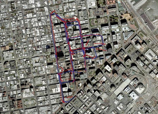
FIGURE1. Conventional test drive (two receivers)
Conventional Testing Methods
Traditionally, the simplest way to test the real-world performance of a GNSS receiver is to put it in a vehicle or a portable pack; drive or walk around an area of interest (typically a challenging environment such as an “urban canyon”); record position data; plot the trajectory on a map; and evaluate it visually. An example of this is shown in Figure 1 for two receivers, in this case driven through the difficult radio environment of downtown San Francisco.
While appealing in its simplicity and direct visual representation of the test drive, this approach does not allow for any quantitative assessment of receiver performance; judging which receiver is “better” is inherently subjective here. Different receivers often have different strong and weak points in their tracking and navigation algorithms, so it can be difficult to assess overall performance, especially over the course of a long trial. Also, an accurate evaluation of a trial generally requires some first-hand knowledge of the test area; unless local maps are available in sufficiently high resolution, it may be difficult to tell, for example, how accurate a trajectory along a wooded area might be.
In Figure 2, it appears clear enough that the test vehicle passed down a narrow lane between two sets of buildings during this trial, but it can be difficult to tell how accurate this result actually is. As will be demonstrated below, making sense of a situation like this is essentially beyond the scope of the simple “visual plotting” test method.
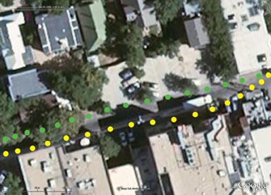
FIGURE 2. Test result requiring local knowledge to interpret correctly.
To address these shortcomings, the simple test method can be refined through the introduction of a GNSS/INS truth reference system. This instrument combines the absolute position obtainable from GNSS with accurate relative measurements from a suite of inertial sensors (accelerometers, gyroscopes, and occasionally magnetometers) when GNSS signals are degraded or unavailable. The reference system is carried or driven along with the devices under test (DUTs), and produces a truth trajectory against which the performance of the DUTs is compared.
This refined approach is a significant improvement over the first method in two ways: it provides a set of absolute reference positions against which the output of the DUTs can be compared, and it enables a quantitative measurement of position accuracy. Examples of these two improvements are shown in Figure 3 and Figure 4.
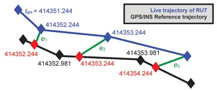
FIGURE 3. Improved test with GPS/INS truth reference: yellow dots denote receiver under test; green dots show the reference trajectory of GPS/INS.FIGURE 4. Time-aligned 2D error.
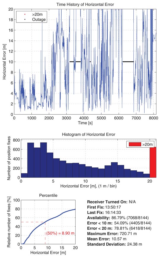
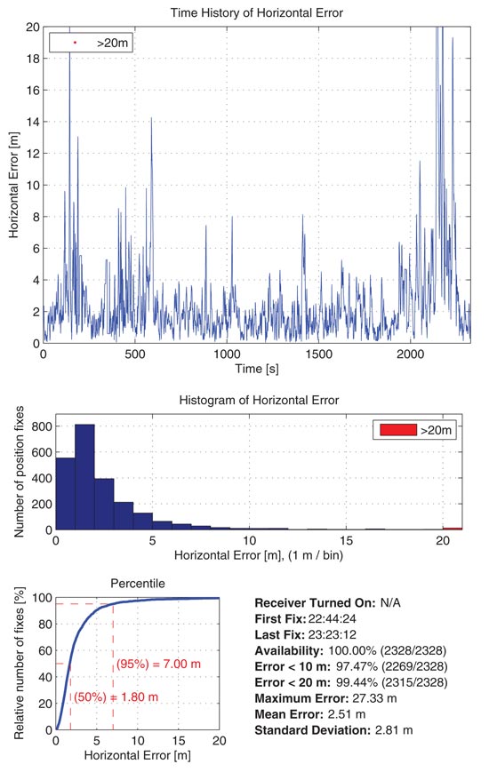
As shown in Figure 4, interpolating the truth trajectory and using the resulting time-aligned points to calculate instantaneous position errors yields a collection of scalar measurements en. From these values, it is straightforward to compute basic statistics like mean, 95th percentile, and maximum errors over the course of the trial. An example of this is shown in Figure 5, with the data (horizontal 2D error in this case) presented in several different ways. Note that the time interpolation step is not necessarily negligible: not all devices align their outputs to whole second boundaries of GPS time, so assuming a typical 1 Hz update rate, the timing skew between a DUT and the truth reference can be as large as 0.5 seconds. At typical motorway speeds, say 100 km/hr, this results in a 13.9 meter error between two points that ostensibly represent the same position. On the other hand, high-end GPS/INS systems can produce outputs at 100 Hz or higher, in which case this effect may be safely neglected.
FIGURE 5. Quantifying error using a truth reference
Despite their utility, both methods described above suffer from two fundamental limitations: results are inherently obtainable only in real time, and the scope of test coverage is limited to the number of receivers that can be fixed on the test rig simultaneously. Thus a test car outfitted with five receivers (a reasonable number, practically speaking) would be able to generate at most five quasi-independent results per outing.
Software Approach
The architecture of a software GNSS receiver is ideally suited to overcoming the limitations described above, as follows.
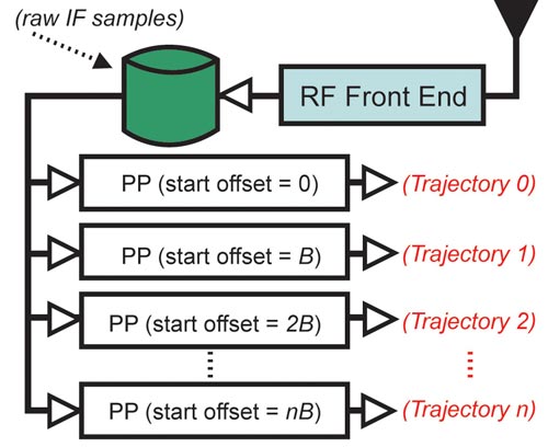
The raw IF data stream from the analog-to-digital converter is recorded to a file during the initial data collection. This file captures the essential characteristics of the RF chain (antenna pattern, downconverter, filters, and so on), as well as the signal environment in which the recording was made (fading, multipath, and so on). The IF file is then reprocessed offline multiple times in the lab, applying the results of careful profiling of various hardware platforms (for example, Pentium-class PC, ARM9-based embedded device, and so on) to properly model the constraints of the desired target platform. Each processing pass produces a position trajectory nominally identical to what the DUT would have gathered when running live. The complete multiple offset post-processi
ng (MOPP) setup is illustrated in Figure 6.
FIGURE 6. Multiple Offset Post-Processing (MOPP).
The fundamental improvement relative to a conventional testing approach lies in the multiple reprocessing runs. For each one, the raw data is processed starting from a small, progressively increasing time offset relative to the start of the IF file. A typical case would be 256 runs, with the offsets uniformly distributed between 0 and 100 milliseconds — but the number of runs is limited only by the available computing resources, and the granularity of the offsets is limited only by the sampling rate used for the original recording. The resulting set of trajectories is essentially the physical equivalent of having taken a large number of identical receivers (256 in this example), connecting them via a large signal splitter to a single common antenna, starting them all at approximately the same time (but not with perfect synchronization), and traversing the test route.
This approach produces several tangible benefits.
The large number of runs dramatically increases the statistical significance of the quantitative results (mean accuracy, 95th percentile error, worst-case error, and so on) produced by the test.
The process significantly increases the likelihood of identifying uncommon (but non-negligible) corner cases that could only be reliably found by far more testing using ordinary methods.
The approach is deterministic and completely repeatable, which is simply a consequence of the nature of software post-processing. Thus if a tuning improvement is made to the navigation filter in response to a particular observed artifact, for example, the effects of that change can be verified directly.
The proposed approach allows the evaluation of error models (for example, process noise parameters in a Kalman filter), so estimated measurement error can be compared against actual error when an accurate truth reference trajectory (such as that produced by the aforementioned GPS/INS) is available. Of course, this could be done with conventional testing as well, but the replay allows the same environment to be evaluated multiple times, so filter tuning is based on a large population of data rather than a single-shot test drive.
Start modes and assistance information may be controlled independently from the raw recorded data. So, for example, push-to-fix or A-GNSS performance can be tested with the same granularity as continuous navigation performance.
From an implementation standpoint, the proposed approach is attractive because it requires limited infrastructure and lends itself naturally to automated implementation. Setting up handful of generic PCs is far simpler and less expensive than configuring several hundred identical receivers (indeed, space requirements and RF signal splitting considerations alone make it impractical to set up a test rig with anywhere near the number of receivers mentioned above). As a result, the software replay setup effectively increases the testing coverage by several orders of magnitude in practice. Also, since post-processing can be done significantly faster than real time on modern hardware, these benefits can be obtained in a very time-efficient manner.
As with any testing method, the software approach has a few drawbacks in addition to the benefits described above. These issues must be addressed to ensure that results based on post-processing are valid and meaningful.
Error and Independence
The MOPP approach raises at least two obvious questions that merit further discussion.
How accurately does file replay match live operation?
Are runs from successive offsets truly independent?
The first question is answered quantitatively, as follows. A general-purpose software receiver (running on an x86-class netbook computer) was driven around a moderately challenging urban environment and used to gather live position data (NMEA) and raw digital data (IF samples) simultaneously. The IF file was post-processed with zero offset using the same receiver executable, incorporating the appropriate system profiling to accurately model the constraints of real-time processing as described above, to yield a second NMEA trajectory. Finally, the two NMEA files were compared using the methods shown in Figure 4 and Figure 5, this time substituting the post-processed trajectory for the GPS/INS reference data. A plot of the resulting horizontal error is shown in Figure 7.
FIGURE 7. Quantifying error introduced by post-processing.
The mean horizontal error introduced by the post-processing approach relative to the live trajectory is on the order of 2.5 meters. This value represents the best accuracy achievable by file replay process for this environment.
More challenging environments will likely have larger minimum error bounds, but that aspect has not yet been investigated fully; it will be considered in future work. Also, a single favorable comparison of live recording against a single replay, as shown above, does not prove that the replay procedure will always recreate a live test drive with complete accuracy. Nevertheless, this result increases the confidence that a replayed trajectory is a reasonable representation of a test drive, and that the errors in the procedure are in line with the differences that can be expected between two identical receivers being tested at the same time.
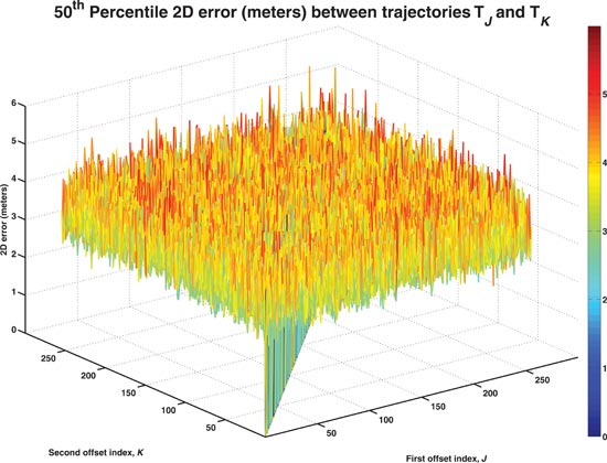
To address the question of run-to-run independence, consider two trajectories generated by post-processing a single IF file with offsets jB and kB, where B is some minimum increment size (one sample, one buffer, and so on), and define FJK to be some quantitative measurement of interest, for example mean or 95th percentile horizontal error. The deterministic nature of the file replay process guarantees FJK = 0 for j = k. Where j and k differ by a sufficient amount to generate independent trajectories, FJK will not be constant, but should be centered about some non-negative underlying value that represents the typical level of error (disagreement) between nominally identical receivers. As mentioned earlier, this is the approximate equivalent of connecting two matched receivers to a common antenna, starting them at approximately the same time, and driving them along the test trajectory.
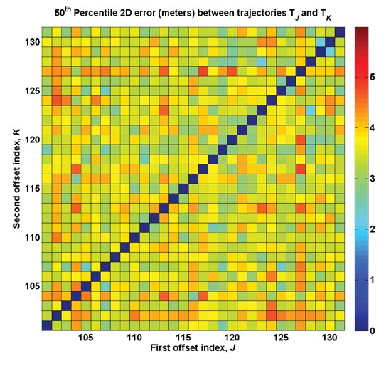
Given these definitions, independence is indicated by an abrupt transition in FJK between identical runs ( j = k) and immediately adjacent runs (|j – k| = 1) for a given offset spacing B. Conversely, a gradual transition indicates temporal correlation, and could be used to determine the minimum offset size required to ensure run-to-run independence if necessary. As shown in Figure 8, the MOPP parameters used in this study (256 offsets, uniformly spaced on [0, 100 msec] for each IF file) result in independent outputs, as desired.
FIGURE 8. Verifying independence of adjacent offsets (upper: full view; lower: zoomed top view)
One subtlety pertaining to the independence analysis deserves mention here in the context of the MOPP method. Intuitively, it might appear that the offset size B should have a lower usable bound, below which temporal correlation begins to appear between adjacent post-processing runs. Although a detailed explanation is outside the scope of this paper, it can be shown that certain architectural choices in the design of a receiver’s baseband can lead to somewhat counterintuitive results in this regard.
As a simple example, consider a receiver that does not forcibly align its channel measurements to whole-second boundaries of system time. Such a device will produce its measurements at slightly different times with respect to the various timing markers in the incoming signal (epoch, subframe, and frame boundaries) for each different post-processing offset. As a result, the position solution at a given time point will differ slightly between adjacent post-processing runs until the offset size becomes smaller than the receiver’s granularity limit (one packet, one sample, and so on), at which point the outputs from successive offsets will become identical. Conversely, altering the starting point by even a single offset will result in a run sufficiently different from its predecessor to warrant its inclusion in a statistical population.
Application-to-Receiver Optimization
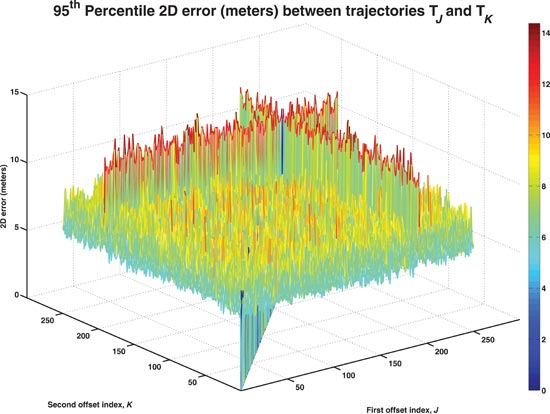
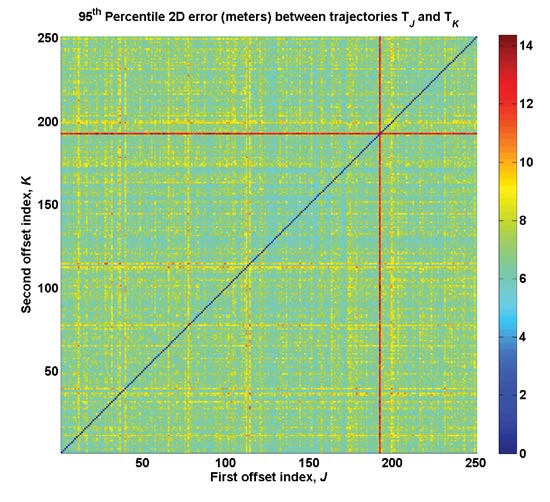
Once the independence and lower bound on observable error have been established for a particular set of post-processing parameters, the MOPP method becomes a powerful tool for finding unexpected corner cases in the receiver implementation under test. An example of this is shown in Figure 9, using the 95th percentile horizontal error as the statistical quantity of interest.
FIGURE 9. Identifying a rare corner case (upper: full view; lower: top view)
For this IF file, the “baseline” level for the 95th percentile horizontal error is approximately 6.7 meters. The trajectory generated by offset 192, however, exhibits a 95th percentile horizontal error with respect to all other trajectories of approximately 12.9 meters, or nearly twice as large as the rest of the data set. Clearly, this is a significant, but evidently rare, corner case — one that would have required a substantial amount of drive testing (and a bit of luck) to discover by conventional methods.
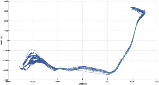
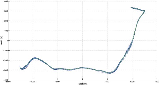
When an artifact of the type shown above is identified, the deterministic nature of software post-processing makes it straightforward to identify the particular conditions in the input signal that trigger the anomalous behavior. The receiver’s diagnostic outputs can be observed at the exact instant when the navigation solution begins to diverge from the truth trajectory, and any affected algorithms can be tuned or corrected as appropriate. The potential benefits of this process are demonstrated in Figure 10.
FIGURE 10. Before (top) and after (bottom) MOPP-guided tuning (blue = 256 trajectories; green = truth)
Limitations
While the foregoing results demonstrate the utility of the MOPP approach, this method naturally has several limitations as well. First, the IF replay process is not perfect, so a small amount of error is introduced with respect to the true underlying trajectory as a result of the post-processing itself. Provided this error is small compared to those caused by any corner cases of interest, it does not significantly affect the usefulness of the analysis — but it must be kept in mind.
Second, the accuracy of the replay (and therefore the detection threshold for anomalous artifacts) may depend on the RF environment and on the hardware profiling used during post-processing; ideally, this threshold would be constant regardless of the environment and post-processing settings.
Third, the replay process operates on a single IF file, so it effectively presents the same clock and front-end noise profile to all replay trajectories. In a real-world test including a large number of nominally identical receivers, these two noise sources would be independent, though with similar statistical characteristics. As with the imperfections in the replay process, this limitation should be negligible provided the errors due to any corner cases of interest are relatively large.
Conclusions and Future Work
The multiple offset post-processing method leverages the unique features of software GNSS receivers to greatly improve the coverage and statistical validity of receiver testing compared to traditional, hardware-based testing setups, in some cases by an order of magnitude or more. The MOPP approach introduces minimal additional error into the testing process and produces results whose statistical independence is easily verifiable. When corner cases are found, the results can be used as a targeted tuning and debugging guide, making it possible to optimize receiver performance quickly and efficiently.
Although these results primarily concern continuous navigation, the MOPP method is equally well-suited to tuning and testing a receiver’s baseband, as well its tracking and acquisition performance. In particular, reliably short time-to-first-fix is often a key figure of merit in receiver designs, and several specifications require acquisition performance to be demonstrated within a prescribed confidence bound. Achieving the desired confidence level in difficult environments may require a very large number of starts — the statistical method described in the 3GPP 34.171 specification, for example, can require as many as 2765 start attempts before a pass or fail can be issued — so being able to evaluate a receiver’s acquisition performance quickly during development and testing, while still maintaining sufficient confidence in the results, is extremely valuable.
Future improvements to the MOPP method may include a careful study of the baseline detection threshold as a function of the testing environment (open sky, deep urban canyon, and so on). Another potentially fruitful line of investigation may be to simulate the effects of physically distinct front ends by adding independent, identically distributed swaths of noise to copies of the raw IF file prior to executing the multiple offset runs.
Alexander Mitelman is GNSS research manager at Cambridge Silicon Radio. He earned his M.S. and Ph.D. degrees in electrical engineering from Stanford University. His research interests include signal quality monitoring and the development of algorithms and testing methodologies for GNSS.
Jakob Almqvist is an M.Sc. student at Luleå University of Technology in Sweden, majoring in space engineering, and currently working as a software engineer at Cambridge Silicon Radio.
Robin Håkanson is a software engineer at Cambridge Silicon Radio. His interests include the design of optimized GNSS software algorithms, particularly targeting low-end systems.
David Karlsson leads GNSS test activities for Cambridge Silicon Radio. He earned his M.S. in computer science and engineering from Linköping University, Sweden. His current focus is on test automation development for embedded software and hardware GNSS receivers.
Fredrik Lindström is a software engineer at Cambridge Silicon Radio. His primary interest is general GNSS software development.
Thomas Renström is a software engineer at Cambridge Silicon Radio. His primary interests include developing acquisition and tracking algorithms for GNSS software receivers.
Christian Ståhlberg is a senior software engineer at Cambridge Silicon Radio. He holds an M.Sc. in computer science from Luleå University of Technology. His research interests include the development of advanced algorithms for GNSS signal processing and their mapping to computer architecture.
James Tidd is a senior navigation engineer at Cambridge Silicon Radio. He earned his M.Eng. from Loughborough University in systems engineering. His research interests
include integrated navigation, encompassing GNSS, low-cost sensors, and signals of opportunity.
Seven technologies that put GPS in mobile phones around the world — the how and why of location’s entry into modern consumer mobile communications.
By Frank van Diggelen, Broadcom Corporation
Exactly a decade has passed since the first major milestone of the GPS-mobile phone success story, the E-911 legislation enacted in 1999. Ensuing developments in that history include:
Snaptrack bought by Qualcomm in 2000 for $1 billion, and many other A-GPS startups are spawned.
Commercial GPS receiver sensitivity increases roughly 30 times, to 2150 dBm (1998), then another 10 times, to 2160 dBm in 2006, and perhaps another three times to date, for a total of almost 1,000 times extra sensitivity. We thought the main benefit of this would be indoor GPS, but perhaps even more importantly it has meant very, very cheap antennas in mobile phones. Meanwhile:
Host-based GPS became the norm, radically simplifying the GPS chip, so that, with the cheap antenna, the total bill of materials (BOM) cost for adding GPS to a phone is now just a few dollars!
Thus we see GPS penetration increasing in all mobile phones and, in particular, going towards 100 percent in smartphones.
This article covers the technology revolution behind GPS in mobile phones; but first, let’s take a brief look at the market growth. This montage gives a snapshot of 28 of the 228 distinct Global System for Mobile Communications (GSM) smartphone models (as of this writing) that carry GPS.
Back in 1999, there were no smartphones with GPS; five years later still fewer than 10 different models; and in the last few years that number has grown above 200. This is that rare thing, often predicted and promised, seldom seen: the hockey stick!
The catalyst was E-911 — abetted by seven different technology enablers, as well as the dominant spin-off technology (long-term orbits) that has taken this revolution beyond the cell phone.
In 1999, the Federal Communications Commission (FCC) adopted the E-911 rules that were also legislated by the U.S. Congress. Remember, however, that E-911 wasn’t all about GPS at first.
It was initially assumed that most of the location function would be network-based. Then, in September 1999, the FCC modified the rules for handset technologies. Even then, assisted GPS (A-GPS) was only adopted in the mobile networks synchronized to GPS time, namely code-division multiple access (CDMA) and integrated digital enhanced network (iDEN, a variant of time-division multiple access).
The largest networks in the world, GSM and now 3G, are not synchronized to GPS time, and, at first, this meant that other technologies (such as enhanced observed time difference, now extinct) would be the E-911 winners. As we all now know, GPS and GNSS are the big winners for handset location. E-911 became the major driver for GPS in the United States, and indirectly throughout the world, but only after GPS technology evolved far enough, thanks to the seven technologies I will now discuss.
Technology #1. Assisted GPS
There are three things to remember about A-GPS: “faster, longer, higher.” The Olympic motto is “faster, stronger, higher,” so just think of that, but remember “faster, longer, higher.”
The most obvious feature of A-GPS is that it replaces the orbit data transmitted by the satellite. A cell tower can transmit the same (or equivalent) data, and so the A-GPS receiver operates — faster.
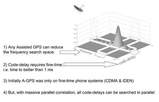
The receiver has to search over a two-dimensional code/frequency space to find each GPS satellite signal in the first place. Assistance data reduces this search space, allowing the receiver to spend longer doing signal integration, and this in turn means higher sensitivity (Figure 1). Longer, higher.
FIGURE 1. A-GPS: reduced search space allows longer integration for higher sensitivity.
Now let’s look at this code/frequency search in more detail, and introduce the concepts of fine time, coarse time, and massive parallel correlation. Any assistance data helps reduce the frequency search. The frequency search is just as you might scan the dial on a car radio looking for a radio station — but the different GPS frequencies are affected by the satellite motion, their Doppler effect. If you know in advance whether the satellite is rising or setting, then you can narrow the frequency-search window.
The code-delay is more subtle. The entire C/A code repeats every millisecond. So narrowing the code-delay search space requires knowledge of GPS time to better than one millisecond, before you have acquired the signal. We call this “fine-time.”
Only two phone systems had this time accuracy: CDMA and iDEN, both synchronized to GPS time. The largest networks (GSM, and now 3G) are not synchronized to GPS time. They are within 62 seconds of GPS time; we call this “coarse-time.” Initially, only the two fine-time systems adopted A-GPS. Then came massive parallel correlation, technology number two, and high sensitivity, technology number three.
#2, #3. MPC, High Sensitivity
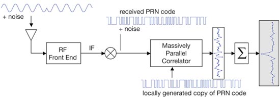
A simplified block diagram of a GPS receiver appears in Figure 2. Traditional GPS (prior to 1999) had just two or three correlators per channel. They would search the code-delay space until they found the signal, and then track the signal by keeping one correlator slightly ahead (early) and one slightly behind (late) the correlation peak. These are the so-called “early-late”correlators.
FIGURE 2. Massive parallel correllation.
Massive parallel correlation is defined as enough correlators to search all C/A code delays simultaneously on multiple channels. In hardware, this means tens of thousands of correlators. The effect of massive parallel correlation is that all code-delays are searched in parallel, so the receiver can spend longer integrating the signal whether or not fine-time is available.
So now we can be faster, longer, higher, regardless of the phone system on which we implement A-GPS.
Major milestones of massive parallel correlation (MPC):
In 1999, MPC was done in software, the most prominent example being by Snaptrack, who did this with a fast Fourier transform (FFT) running on a digital signal processor (DSP). The first chip with MPC in hardware was the GL16000, produced by Global Locate, then a small startup (now owned by Broadcom).
In 2005, the first smartphone implementation of MPC: the HP iPaq used the GL20000 GPS chip. Today MPC is standard on GPS chips found in mobile phones.
#4. Coarse-Time Navigation
We have seen that A-GPS assistance relieves the receiver from decoding orbit data (making it faster), and MPC means it can operate with coarse-time (longer, higher).
But the time-of-week (TOW) still needed to be decoded for the position computation and navigation: for unambiguous pseudoranges, and to know the time of transmission. Coarse-time navigation is a technique for solving for TOW, instead of decoding it. A key part of the technique involves adding an extra state to the standard navigation equation, and a corresponding extra column to the well known line-of-sight matrix.
The technical consequence of this technique is that you can get a position faster than it is possible to decode TOW (for example, in one, two, or three seconds), or you can get a position when the signals are too weak to decode TOW. And a practical consequence is longer battery life: since you can get fast time-to-first-fix (TTFF) always, without frequently waking and running the receiver to maintain it in a hot-start state.
#5. Low Time-of-Week
A parallel effort to coarse-time navigation is low TOW decode, that is, lowering the threshold at which
it is possible to decode the TOW data. In 1999, it was widely accepted that -142 dBm was the lower limit of signal strength at which you could decode TOW. This is because -142 dBm is where the energy in a single data bit is just observable if all you do is integrate for 20 ms.
However, there have evolved better and better ways of decoding the TOW message, so that now it can be done down to -152 dBm. Today, different manufacturers will quote you different levels for achievable TOW decode, anywhere from -142 to -152 dBm, depending on who you talk to. But they will all tell you that they are at the theoretical minimum!
#6, #7. Host-Based GPS, RF-CMOS
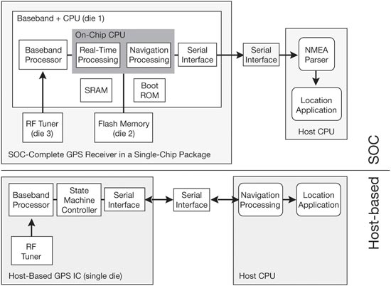
Host-based GPS and RF-CMOS are technologies six and seven, if you’re still counting with me. We can understand the host-based architecture best by starting with traditional system-on-chip (SOC) architecture. An SOC GPS may come in a single package, but inside that package you would find three separate die, three separate silicon chips packaged together: A baseband die, including the central processing unit (CPU); a separate radio frequency tuner; and flash memory. The only cost-effective way of avoiding the flash memory is to have read-only memory (ROM), which could be part of the baseband die — but that means you cannot update the receiver software and keep up with the technological developments we’ve been talking about. Hence state-of-the-art SOCs throughout the last decade, and to date, looked like Figure 3.
FIGURE 3. Host-based architecture, compared to SOC.
The host-based architecture, by contrast, needs no CPU in the GPS. Instead, GPS software runs on the CPU and flash memory already present on the host device (for example, the smartphone). Meanwhile, radio-frequency complementary metal-oxide semi-conductor (RF-CMOS) technology allowed the RF tuner to be implemented on the same die as the baseband. Host-based GPS and RF- CMOS together allowed us to make single die GPS chips.
The effect of this was that the cost of the chip went down dramatically without any loss in performance.
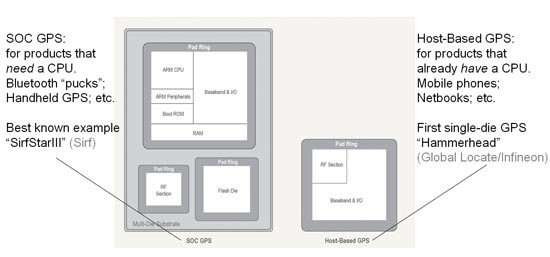
Figure 4 shows the relative scales of some of largest-selling SOC and host- based chips, to give a comparative idea of silicon size (and cost). The SOC chip (on the left) is typically found in devices that need a CPU, while the host-based chip is found in devices that already have a CPU.
FIGURE 4. Relative sizes of host-based, compared to SOC.
In 2005, the world’s first single-die GPS receiver appeared. Thanks to the single die, it had a very low bill of materials (BOM) cost, and has sold more than 50 million into major-brand smartphones and feature phones on the market.
Review
We have seen that E-911 was the big catalyst for getting GPS into phones, although initially only in CDMA and iDEN phones. E-911 became the driver for all phones once GPS evolved far enough, thanks to the seven technology enablers:
A-GPS >> faster, longer, higher
Massive parallel correlation >> longer, higher with coarse-time
High-sensitivity >> cheap antennas
Coarse time navigation >> fast TTFF without periodic wakeup
Low TOW >> decode from weak signals
Host-based GPS, together with
RF-CMOS g single die.
Meanwhile, as all this developed, several important spin-off technologies evolved to take this technology beyond the mobile phone. The most significant of all of these was long-term orbits (LTO), conceived on May 2, 2000, and now an industry standard.
Long-Term Orbits
Why May 2, 2000? Remember what happened on May 1, 2000: the U.S. government turned off selective availability (SA) on all GPS satellites. Suddenly it became much easier to predict future satellite orbits (and clocks) from the observations made by a civilian GPS network. At Global Locate, we had just such a network for doing A-GPS, as illustrated in Figure 5. On May 2 we said, “SA is off — wow! What does that mean for us?”And that’s where LTO for A-GPS came from.
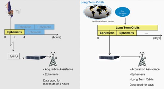
FIGURE 5. Broadcast ephemeris and long-term orbits.
Figure 5 shows the A-GPS environment with and without LTO. The left half shows the situation with broadcast ephemeris only. An A-GPS reference station observes the broadcast ephemeris and provides it (or derived data) to the mobile A-GPS receiver in your mobile phone. The satellite has the orbits for many hours into the future; the problem is that you can’t get them.
The blue and yellow blocks in the diagram represent how the ephemeris is stored and transmitted by the GPS satellite. The current ephemeris (yellow) is transmitted; the future ephemeris (blue) is stored in the satellite memory until it becomes current. So, frustratingly, even though the future ephemeris exists, you cannot ordinarily get it from the GPS system itself.
The right half of the figure shows the situation with LTO. If a network of reference stations observes all the satellites all the time, then a server can compute the future orbits, and provide future ephemeris to any A-GPS receiver. Using the same color scheme as before, we show here that there are no unavailable future orbits; as soon as they are computed, they can be provided. And if the mobile device has a fast-enough CPU, it can compute future orbits itself, at least for the subset of satellites it has tracked.
Beyond Phones. This idea of LTO has moved A-GPS from the mobile phone into almost any GPS device. Two of most interesting examples are personal navigation devices (PNDs) in cars, and smartphones themselves that continue to be useful gadgets once they roam away from the network. Now, of course, people were predicting orbits before 2000 — all the way back to Newton and Kepler, in fact. It’s just that in the year 2000, accurate future GPS orbits weren’t available to mobile receivers. At that time, the International GNSS Service (IGS) had, as it does now, a global network of reference stations, and provided precise GPS orbits organized into groups called Final, Rapid and Ultra-Rapid. The Ultra-Rapid orbit had the least latency of the three, but, in 2000, Ultra-Rapid meant the recent past, not the future.
So for LTO we see that the last 10 years have taken us from a situation of nothing available to the mobile device, to today where these long-term orbits have become codified in the 3rd Generation Partnership Project (3GPP) and Secure User Plane Location (SUPL) wireless standards, where they are known as “ephemeris extension.”
Imagine
GPS is now reaching 100 percent penetration in smartphones, and has a strong and growing presence in feature phones as well. GPS is now in more than 300 million mobile phones, at the very least; credible estimates range above 500 million.
Now, imagine every receiver ever made since GPS was created 30 years ago: military and civilian, smart-bomb, boat, plane, hiking, survey, precision farming, GIS, Bluetooth-puck, personal digital assistant, and PND. In the last three years, we have put more GPS chips into mobile phones than the cumulative number of all other GPS receivers that have been built, ever!
Frank van Diggelen has worked on GPS, GLONASS, and A-GPS for Navsys, Ashtech, Magellan, Global Locate, and now as a senior technical director and chief navigation officer of Broadcom Corporation. He has a Ph.D. in electrical engineering from Cambridge University, holds more than 45 issued U.S. patents on A-GPS, and is the author of the textbook A-GPS: Assisted GPS, GNSS, and SBAS.
Recent attention given to aging GPS satellites and availability gaps from lagging constellation replenishment have provoked deep concern, particularly within the aviation community. Available remedies include exploitation of well known but unused methods plus new techniques; those discussed here have future relevance, with or without availability gaps.
Even with far greater coverage from multiple GNSS, crises could emerge from severely stronger interference levels or other unforeseen events. Advance preparation for any such occurrence would avoid the waste, confusion, and blind alleys that generally arise with the sudden appearance of an emergency.
GPS lives up to expectations, brilliantly performing as advertised. Even that best-ever performance must and does have tolerance for occasional error; examples, though rare, are well documented. To live with less than perfect performance, the industry relies on integrity testing: comparison checks using extra satellites to detect inconsistencies and exclude questionable data.
Nevertheless, it is universally recognized that GNSS, even with existing fault detection and isolation or exclusion (FDI/FDE), is still not perfect. The ramifications of growing dependence on GPS have thus attracted more attention. The overall subject can be subdivided into general areas involving the likelihood of:
reduced availability and
reduced dependability (integrity, its verification, plus backup).
Although I mainly address the first topic here, the second unavoidably intertwines itself, making it difficult to keep them separate. Despite wide acclaim for the excellent 2001 Volpe Report, commitment to a key means of backup for GPS remains unclear at this time. Possibility of a shortfall calls for a review of both existing methods and procedures, and possible means for closing the gap.
Current Methods
Today’s air traffic management designs demand constant replenishment of instantaneous position by full fixes.
Full Fix 1 RAIM. When each data vector must be a self-sufficient source of instantaneous position, a requirement arises for enough satellite sightline directions with geometric spread at all times. That interdependence is magnified when more satellites are added to provide FDI/FDE, requiring every subset of four within the enlarged group to support the requisite geometry. With this all-or-nothing posture, data lapses form a major stumbling block. A data gap that is only partial equates to a loss of GPS.
Position-Oriented Approach. Especially at high speeds, as in flight, instantaneous position is highly perishable. With little or no emphasis placed on accurate dynamics (beginning with velocity), demand for continuously accurate instantaneous position is highly dependent on abundant data. That abundance includes sufficiently high data rates, since latency becomes a significant liability without usage of a dynamic file.
Carrier Phase (Classical). Successful use of carrier-phase information is decades old. Although ambiguity resolution is not required in all carrier-phase applications, requirements for cycle-slip detection are quite common. More common yet — in fact, virtually ubiquitous — is the need to maintain phase continuity via a carrier-track loop. When those needs are satisfied, sub-wavelength instantaneous position is obtainable. Challenges involved, however, have produced among users a wide variation in perception of value. Some negative perceptions have arisen due to cutting corners in formation of carrier phase, or merely settling for delta range, by some receivers. Further, a cycle slip, even if only rarely overlooked, can be catastrophic in some operations.
Imperfect Validation. As already noted, verification is not my main topic here, but the issue is inescapable. Shortcomings include hard evidence of certification improperly bestowed, and severe limitations of go/no-go criteria (as with an automobile’s dashboard warning lights, we can learn if a performance trait is unsatisfactory — but a trivial excess produces the same indication as an imminent danger).
Necessary Changes
Extremely powerful and versatile means to improve performance have been available for a very long time. Kalman’s original paper, half a century ago, formalized an optimal way to achieve such performance. While Kalman estimation is commonly used today, its effective reach is almost invariably limited to data resident within each proprietary box of equipment.
The resources for providing centrally processed solutions for data from every source of information available, any combination of sources, any subset that may exclude any sensor or group, or any individual source in a federated configuration, are well known. Every conceivable choice from among these solutions can be made concurrently available; note the inherent backup.
However, all this capability is forsaken or lost by continued use of:
interfaces chosen poorly or from outdated standards;
undue consolidation within isolated equipment packaging;
overextended proprietary rights; and
limited, demonstrably flawed validation methods.
Drop Demands for Full Fix. An immediate explosion of benefits can follow from acceptance of partial information. Countless examples could be cited, but two obvious ones suffice:
Within GPS or GNSS, not all space vehicles (SVs) would be simultaneously affected by scintillation; ionospheric disturbance effects vary with both location and time. A similar case holds for multipath. Data from some SVs could be rejected, by decisions made external to a receiver, without forcing rejection of all.
Central processing — not within any one equipment box — has always offered potential for other sources (distance-measuring equipment or DME, and so on) to make up for incomplete sets of SV data.
My broad goal here is to take advantage of information not currently used and to prescribe corrective strategies. That objective has not been widely pursued due to perceived lack of urgency. GPS availability has thus far been more than satisfactory to a multitude of users — but that could change.
Availability Enhancements. For about two decades, the industry was effectively guided by a strong preference for the trait whereby every data refresh event was self-sufficient. A major reason for this was protection against gradual veering: a snapshot sequence is less sensitive than a continuously evolving path estimate. The cost, of course, is forfeit of benefits conferred by the sequence’s history. More recently, a middle ground was sought to mitigate the resulting loss; subfilters used as much new data as possible while making some use of knowledge from an estimator’s covariance matrix.
I promptly endorsed that approach and sought to carry it to the limit. A single-measurement receiver-autnomous integrity monitoring (RAIM) resulted, offering an independent integrity test for each separate observation. Despite its rigorous derivation, the technique is quite simple in practice. Further, it bridges a gap that formerly separated integrity test from optimal estimation, while also having significant advantages over conventional RAIM:
separation translates to independence from other satellites, and therefore from geometry (effective DOP of unity)
ability to use different error variances for different observations (for example, with nonuniformity in signal strength and/or elevation).
With this discussion, we have clearly left the realm of well-known subjects with self-evident prescriptions. Much of what follows likewise falls into the category of relatively obscure methods.
Beyond Position-Oriented. A time history
of GNSS observations, with or without an inertial measurement unit (IMU), inherently carries dynamic information. A file with observational history from multiple sources of course enables the aforementioned explosion of benefits. The obvious immediate offerings include:
closing of data lapses via information sharing;
intrinsic backup with automatic activation;
vast reduction of latency effects (for example, from 200 meters to less than 1 meter at 400 knots after 1 second, with easily obtainable velocity accuracy below 1 meter/second);
formation of 1-sigma projected future error (within reason).
Beyond these lie, once again, some lesser known techniques, including a few that are virtually nonexistent in operation at the time of this writing. With GNSS, the full potential of dynamics calls for a revisit of carrier phase.
Carrier-Phase Developments. Rather than pursuit of unnecessary sub-wavelength fixes for aircraft (for example, with 20-meter wing span moving at 400 knots), the true value of carrier phase in flight lies in enhanced dependability. Sequential changes in carrier phase over 1 second provide excellent dynamics information, with or without an IMU.
Recognition of this opportunity led to the concept of segmentation, whereby position is determined separately from dynamics. Carrier-phase sequential changes with ambiguities unresolved can provide precise (1-centimeter/second RMS with IMU; decimeter/second without) streaming velocity independent of position. Dead reckoning then provides a priori position correctible by pseudoranges.
One advantage of this scheme is subtle: with 1-second phase change propagation effects generally at 1 centimeter or less, no mask is needed. The geometry benefit is obvious, and flight experience has verified it. This raises another segmentation characteristic: the single-measurement integrity testing is applicable to each carrier-phase sequential change and to each pseudorange, separately and independently.
These capabilities are untapped in essentially all operational systems — air, land, and sea — and all stand to gain. Yet another opportunity can be added: ability to sustain operation even if every SV has repetitive data gaps. This advantage is best exploited with receivers described next.
FFT-Based Processing. Correlators and track loops in GNSS receivers can be replaced. The theory is age-old: multiplication in the frequency domain corresponds to convolution in time (and vice-versa). Thus a term-by-term product of a digitized receiver input’s fast Fourier transform (FFT) with the reference pattern’s FFT can, after an inverse FFT, provide outputs equivalent to full sets of correlator responses. Today’s processing and analog-to-digital converter capabilities offer feasibility.
In addition to reduced vulnerability to jamming (not covered here), advantages include:
access to all cells (not only a track loop’s subset)
guaranteed access (stability is not conditional)
linear phase-versus-frequency; no phase distortion.
Features from the preceding section, combined with these traits, offer extreme robustness.
Extension to Surveillance. The practice of transmitting responses to RF interrogations has, for many decades, been quite vulnerable to overload (garble; one user’s information is everyone else’s interference). One report described the unsurprisingly poor performance during the first Gulf War, and identified a remedy: squitters with separate assigned time slots, spontaneously firing the transponder transmitter without interrogation. Immediately, a sea change in capability offers every participant an opportunity to track every other participant. With no interrogations, garble would disappear.
This dramatic increase in capacity has been successfully demonstrated with the use of an existing communication link and existing airborne equipment: GPS receivers and Mode S squitters. Subsequently I enthusiastically advocated adoption of the technique with one fundamental modification: replace the data bits of the transmitted messages with measurements instead of coordinates.
Additional improvements include small shifts in time (reducing bits needed for time tags) and recomputation of measurements that would have occurred at the center of gravity (to mitigate rotation effects). Collectively, the full set of procedures offers a vast and compelling list of benefits.
Conclusions
Capability and dependability of navigation and surveillance can be enormously increased. The key lies not in new inventions nor provisions, but in use of newer methods, (among them, FFT-based receivers, segmented estimation, and 1-second carrier-phase changes) while abandoning habits such as:
dismissal of partial fix data
preoccupation with full fixes for instantaneous position irrespective of dynamics
preference for location pseudomeasurements rather than the measurements themselves
reliance on proprietary software in equipment boxes
RF interrogation/response sequences instead of squitters.
The industry can either adopt changes or continue to settle for performance levels at a minor fraction of the intrinsic capabilities available from our present and future systems.
James L. Farrell worked for 31 years at Westinghouse in design, simulation, and validation of navigation and tracking programs. He continues teaching and consulting for private industry, the Department of Defense, and university research through Vigil, Inc
Few precise-positioning users have employed Loran in a professional sense, although maybe you have in your personal life if you’re a airplane pilot or a mariner. Then again, if you’ve flown as an airline passenger or cruised onboard a ship, you’ve benefited from the back-up to GPS that Loran provides. Similarly, if you’ve used a mobile phone recently; you don’t see it, but the wireless carriers all use Loran as a back-up. That back-up is about to go away.
Loran was developed initially for marine navigation and then adopted for aviation navigation. I used Loran-C for aviation navigation in the early 90’s after I earned my private pilot’s license. It was much easier than triangulating off of VORs and NDBs. Yes, GPS receivers for aviation were starting to emerge at that time but flying is expensive so a hand-held GPS was an out-of-reach luxury for a newlywed who just bought his first house and was preparing to start a family.
Loran is a terrestrial (ground-based) system of broadcasting towers, somewhat synonymous with NDGPS. You can read details about the system in the link I provided, but essentially it’s a line-of-sight system in which the Loran receiver antenna needs a direct path to the tower to utilize the signal. Coverage depends on the density of the broadcasting towers. Some regions are covered better than others and when I was using it, there were many areas that were not covered. Accuracy is always an ambiguous subject with respect to navigation technologies, so I’ll go out on a limb and say that Loran-C accuracy is repeatable to about 20 meters. A proposal was floated to upgrade Loran to a system called e-Loran which is reportedly accurate to about 9 meters.
Anyway, over the past several years there’s been a discussion about what to do with the Loran system because it’s clear that GPS has supplanted Loran as the primary navigation system for marine and aviation. Several articles have been published in GPS World by industry experts with most being in favor of maintaining Loran. The primary argument is that we need a back-up system for GPS, not only for navigation, but for the many invisible ways that GPS supports the national infrastructure (financial networks, wireless communications, transportation).
Here are several relevant articles, from most recent to further back:
The Case for eLoran In addition to these articles , the U.S. government publishes the Federal Radionavigation Plan (FRP) roughly on a biennial basis. There was one published in 2001, then 2005 and the last one was published in 2008/early 2009. It is the official policy document in which all US navigation systems are planned. According to the FRP, it is prepared jointly by the Department of Defense, Department of Homeland Security, the Department of Transportation and a number of other contributing government agencies.
If you don’t have time to read the 2008 FRP, following is a telling statement from the document:
“In March 2007, the DOT Pos/Nav Executive Committee and the DHS Geospatial/PNT Executive Committee accepted the findings of the Institute for Defense Analysis’ Independent Assessment Team and approved to pursue the designation of Enhanced-Loran, commonly referred as eLoran, as a national PNT backup for the U.S. homeland.
At its March 2007 meeting, the National Space-based PNT ExComm supported this approach and tasked DOT and DHS to complete an action plan that includes identifying an executive agent, developing a transition plan to address funding and operations and requesting the approval by the DOT and DHS Secretaries resulting in a final decision. DoD has not approved eLoran as a GPS backup for military applications.
In March 2008, the National Space-based PNT ExComm endorsed the DOT/DHS decision to transition the LORAN system to eLoran.
With respect to transportation to include aviation, commercial maritime, rail, and highway, the DOT has determined that sufficient alternative navigation aids currently exist in the event of a loss of GPS-based services, and therefore Loran currently is not needed as a back-up navigation aid for transportation safety-of-life users. However, many transportation safety-of-life applications depend on commercial communication systems and DOT recognizes the importance of the Loran system as a backup to GPS for critical infrastructure applications requiring precise time and frequency.
Currently, DHS is determining whether alternative backups or contingency plans exist across the critical infrastructure and key resource sectors identified in the National Infrastructure Protection Plan in the event of a loss of GPS-based services. An initial survey of the Federal critical infrastructure partners indicates wide variance in backup system requirements. Therefore, DHS is working with Federal partners to clarify the operational requirements.”
By the way, that Independent Assessment Team mentioned in the first paragraph was led by Brad Parkinson, who knows someting about GPS. Further, the government read the report behind closed doors but refused to release it, until forced to do so nearly two years later, by public information access filings.
There still aren’t any answers to the question about a real back-up to GPS. No doubt it’s a vulnerable system. But that’s a subject for another day.
What’s Loran got to do with us?
The reason I’m writing about this is because as support for Loran wanes, attention (resources and focus) shifts away from Loran, it comes to bear more intensely on GPS navigation and its augmentations for marine and aviation; specifically DGPS and SBAS (WAAS/EGNOS/MSAS).
With a significant policy shift such as this (albeit it has been in the cards), manufacturers stop allocating engineering development resources to the products/technologies with a dim future and shift those resources to products/technologies with a bright future. True, DGPS has been around for better than a decade and SBAS for about half that time so there’s been plenty of time for manufacturer’s to exploit those technologies, but there is still a lot that can be done.
Engineers are experimenting with and implementing technologies in some interesting areas.
HA-NDGPS. High accuracy NDGPS. Currently with a high performance DGPS receive
r, one can attain about meter-level accuracy. Testing with HA-NDGPS, using a dual frequency GPS receiver shows that accuracies in the 10cm (95%) horizontal and 20cm (95%) vertical range are achievable within a 100 mile baseline according to the US DOT Federal Highway Administration Turner-Fairbank Research Center. Test broadcasts are being sent from a site in Hagerstown, MD.
Broadcasting DGPS/SBAS corrections via NTRIP. The emergence of RTK Networks has spurred the popularity of using the internet to deliver GPS corrections. NTRIP has become a commonly used method of accomplishing this. One of the weak points of DGPS technology has been the reliability and expense of broadcasting DGPS corrections via the 283-325kHz band. Of course, with NTRIP one must have internet access somehow and that typically happens via WiFi or GSM/CDMA mobile phone network. But it’s not that complicated. I’ve been with a GPS user who has pulled the SIM card from their iPhone, plugged it into a GPS receiver, and begin receiving DGPS corrections immediately.
During my last webinar, someone had posed the question if receiving SBAS corrections is possible via the internet in order to bypass the requirement to maintain visibility of the SBAS geostationary satellite. Streaming SBAS corrections via the internet is already happening in Europe. Users can access EGNOS corrections and bypass the EGNOS geostationary satellites by using SISNeT. A similar type of system could be implemented for any SBAS and not necessarily by the SBAS service provider. It could be a commercial entity.
I think the internet and GSM/CDMA mobile phone networks are really going to transform the way we transport data from reference stations to our receivers in the field. We’ve been fighting this battle of delivering GPS corrections for better than a decade. In the past, we’ve experimented with FM pagers and landline modems and now we’ve settled on low frequency radiobeacon, VHF/UHF/Spread spectrum and geostationary satellites but none are close to the perfect solution. GSM/CDMA mobile phone networks may be the final solution as the networks continue to build-out towards complete geographic coverage. Of course, we are helped immensely by the mobile phone industry whose focus on data for the many new social networking applications will drive the price of data plans downward.
By the way, almost all wireless carriers use Loran as a back-up technology; highly precise timing is a key aspect of how wireless communication works. The carriers use GPS for that, but if GPS goes down — as it did in San Diego during a memorable jamming episode a few years ago — so do all cell phones, if the carriers don’t have a timing back-up. In San Diego, they didn’t. Just something to think about, if you are using your mobile phone network to transport data or receive corrections.
I received some feedback on my last column entitled “What’s the Difference Between a Used Car Salesman and a GPS Salesman?” Most of the comments were positive in that the technical content was reasonably deep and thorough. However, I did receive a couple of e-mails from folks who were offended by the comparison.
The joke has been around for a long time. As I mentioned, I recall hearing it in the early ’90s. I believe it was while I was at a conference somewhere in British Columbia, Canada. Anyway, I used to be a GPS salesman of sorts and I never took offense to it. I figured if I was doing my job correctly, there was nothing to be offended by. But, the fact is the joke has maintained staying power because a number of people do exist who fit that description. Fortunately, they don’t seem to hang around very long in the industry. On the flip side, over the years I’ve met many competent GPS sales professionals that have earned my trust. Many of whom I consider my friends.
Leftover Webinar Q&A
There are some lingering questions left over from the last webinar (September). There are still a few questions left after this that I’ll post in future newsletters.
Question #1: If GLONASS has a full constellation by 2020, would it be fair to say a L1, L2, and GLONASS receiver would be fine because you would really only have a L1 and GLONASS receiver thus therefore enough sats?
Gakstatter: The question is referring to the semicodeless sunset I’ve written about in the past. You can read about it here.
Back to the question. Generally speaking, I would say yes but it’s going to depend on the receiver firmware design. If the receiver is optimized to depend on L2, then the firmware would have to be altered. Then, the question is whether the manufacturer is willing to update the firmware.
Question #2: If SBAS is made for aviation safety purposes, why it does not cover all of the world? Will the coverage expand in the future?
Gakstatter: Building an SBAS is very expensive and time-consuming project. If I recall correctly, the US WAAS total expenditure to date is well into several billion dollars. The FY2010 annual budget for WAAS is just under US$100M.
The nature of SBAS is that they are regional systems. Currently, there are three. WAAS covers most of North America. EGNOS covers most of Western Europe and North Africa. MSAS covers the region around Japan. GAGAN is still in the planning stage and will cover India and surrounding areas.
This still leaves South America, Australia, and Africa as major land masses not covered by SBAS.
MSAS has the potential to cover Australia and EGNOS has the potential to cover Africa. Whether that happens or not is more political and financial than technical issues.
Also, once GPS L5 is broadcast by a full constellation, the requirement for SBAS for aviation will diminish because GPS in aviation will transition to dual frequency (L1/L5) thus mitigating the effects of the ionosphere. However, there would still be a question about position integrity, which is a central function of SBAS. The debate within some countries that do not currently have SBAS coverage is whether to invest in a SBAS or hold out for GPS L5. However, a full satellite constellation broadcasting GPS L5 will not be operational until ~15 years from now.
Question #3: Can we obtain SBAS in other regions in the future?
Gakstatter: India is far along with their GAGAN SBAS. At one point, a test signal was being broadcast. Within the next few months, India reportedly will be launching a geostationary satellite for GAGAN.
Russia is reportedly in the early stages of developing their SBAS called SDCM (System of Differential Correction and Monitoring).
The interoperability among SBAS is virtually seamless. A GPS receiver utilizing WAAS in North America is able to use EGNOS in Europe and MSAS in the Japanese region. Most receivers will automatically tune to the local SBAS given the SBAS satellites in view. However, some must be manually set to “look” for the SBAS satellite(s) of that region.
Question #4: GNSS improves the productivity. What about the precision? Are there any reports testing/comparing GPS vs GNSS?
Gakstatter: At this point, the ideal situation would be to only utilize GPS satellites. The quality, integrity and monitoring is world-class. Unfortunately, for RTK users there just aren’t enough of them in orbit to be able to work consistently throughout the day.
The quality and reliability of GLONASS measurements aren’t as good as GPS yet. The ephemeris data and clock corrections are worse and there isn’t world-wide monitoring of the satellites. Russia’s program managers have stated they are striving to reach the same measurement quality as GPS.
So, the short answer is no, I wouldn’t expect GPS/GLONASS to improve positioning precision. However, it also depends on the scenario. If the comparison is between a GPS constellation of 5 satellites with a PDOP of 5 against a GPS/GLONASS constellation of 5 + 5 with a PDOP of 2, then I’d vote for the latter.
There is an extensive report available from The Survey Assocation in the UK. Although it focuses on Network RTK, there’s a valuable discussion in it regarding GLONASS. You can download the report here.
Question #5: By 2020, is the DOD going to completely get rid of L2 signal?
Gakstatter: No, not at all. L2 was never intended for use by the civilian community. However, in the 1980’s, some really smart scientists in the commercial sector figured out a way to gain access to the encrypted L2 signal via a technique is referred to as semicodeless.
Since that time, the Department of Defense (DOD) has respected that technique because it’s been vitally important in the development of the GPS commercial markets. By respected, I mean they have intentionally not made changes to the GPS that would disrupt the semicodeless technique.
The DOD has now has come to a point that dancing around the semicodeless issue has become a bigger liability than they want to assume. That’s understandable since L2C will allow dual frequency GPS receivers to utilize L2 without using semicodeless techniques, the DOD wants to be released of their liability with respect to L2 semicodeless.
So, after December 31, 2020, the DOD will no longer guarantee that semicodeless receivers will operate as they do today. It is not a “brick wall” in that it will stop working at midnight on December 31, 2020. In fact, a semicodeless receiver may work perfectly fine most of the time after December 31, 2020, but if it stops working properly, the user assumes the liability.
Off-topic
One of the reasons my column is late this week is that I caught a bug earlier this week. It’s nothing serious; it’s just slowing me down a bit because I don’t have the energy I normally have. The fact is that I just don’t get sick beyond my tendency to attract strep throat once every few years.
This year, I’ve opted out of the flu shot despite a specific call from my mother putting the heat on me to get one. I’ve never gotten a flu shot and probably never will. But, I do admit this is the first year I’ve actually considered it. At one point a few weeks ago, 25% of the primary and middle school-aged kids in our school district
were absent due to illness. There were significantly fewer Trick-or-Treaters in our neighborhood this year; I believe due to illness.
I’ve always made an effort to wash my hands, face, nose regularly (no, I’m not obsessive-compulsive) and pay attention to those around me when I’m in public places like malls, movie theaters and airplanes. I absolutely hate getting stuck sitting next to a person on an airplane who is coughing and sneezing. I remember specifically sitting next to a person on a flight back from Phoenix, Arizona, a half-dozen years ago. She looked like death warmed-over…coughing and sneezing horribly. Sure enough, the next day I could feel my body losing the battle. I ended up contracting strep. Ugh.
Anyway, I want to remind you given that many of the US readers are traveling next week for the Thanksgiving holiday to take care of yourselves and your loved ones. You’ll be traveling amongst those who haven’t escaped “the bug,” but have still decided to travel. Here are some tips from the Center for Disease Control and Prevention to keep you and your loved ones healthy.
One of the new initiatives at Geospatial Solutions (GSS) that I mentioned a couple of weeks ago is a Surveying Section on the website. This is an area on the GSS website that’s going to be dedicated to surveyors and GISer’s who want to collaborate. By collaborating, I mean sharing ideas, sharing data, resolving conflicts and generally communicating in a positive way.
“A particular area where I want to pay specific attention is what I call the Survey Section. There is no doubt in my mind that land surveying professionals and GIS professionals are going to be close brethren in the geospatial world. The roles of both are evolving and the line of demarcation is not always clear, but the two need each other terribly in order to best serve the public. GIS isn’t always about parcel maps and land surveying isn’t always about coordinates. The Survey Section (or whatever better name I come up with) will be a place for this sort of knowledge exchange and collaboration in a positive way. There is not one person or company that can stop this geospatial train, so what’s left is how best the two professions can work together.”
In the column title, I refer to RPLS (Registered Professional Land Surveyor) and GISP (Geographic Information System Professional). RPLS is a generic term I use, but actually there are many different titles used depending on which US state or which country you reside in. RPLS roles are defined by each U.S. state statute (or country law) and their role varies widely from state to state and from country to country. For example, their role in California is much more encompassing than in Nevada. Likewise, the RPLS definition from one country to the next can be vastly different. GISP, on the other hand, is a certification of competency. Their role is not defined nor regulated by individual states or countries (that I’m aware of).
RPLS and GISP are formal titles for the licensed (RPLS) and certified (GISP) people in their respective professions. Beyond those who are licensed and certified, there are orders of magnitude more practioners, technicians and specialists who utilize measurement, data collection and data processing technology (hardware and software) in order to complete their tasks at hand. As technology advances and becomes more accessible and more powerful, the growth rate of practioners, technicians and specialists is going to far exceed the growth rate of RPLS and GISP personnel.
How can I make that statement?
The fact is that data collection (hardware/software) and analysis (software) technology is becoming cheaper and easier to use every year. The established guard might think of it as “dumbing down” the profession, but I don’t think it is. Think back 60 years ago when data entry was accomplished via punch cards. Today, it is widely accepted and expected that everyone uses a keyboard to enter data…and they are responsible for their data entry errors.
The result of advancing technology and a tightening economy is that there are many more organizations purchasing the technology and performing certain tasks themselves. So, not only are the roles between the RPLS and GISP getting fuzzier, but also the line of demarcation between the client and the RPLS/GISP.
One example is wetland delineation mapping. In the past, it was common for a wetland scientist to flag the boundary of a wetland and then hire a third party to measure the locations of the flags and create the wetland delineation map. However, it is becoming common for the wetland scientist to carry a GPS mapping receiver with them and map the flags as they are set. This saves the client time by not having to wait for someone else to return to the site and map it. It also saves money by being able to keep the activity in-house. The risk of bringing the activity in-house is having potentially lower quality data if the wetland scientist isn’t well-versed in how to utilize the GPS mapping technology.
One can argue that the line of demarcation is easy to draw…just refer to the local statute. Maybe, but I can see two problems with that:
Advancing technology and expertise have allowed RPLS to extend their scope of services in their businesses. For example, an RPLS firm offers mapping services that aren’t inside the bounds of the local statute (eg. wetland surveys). GPS and GIS technology advancements have stimulated this growth.
In the areas of expertise that fall outside of the local statutes, there ends up being a “turf battle.” In the wetland mapping example above, the wetland scientist may not be an in-house employee. He/she may be a contractor to the client just like the RPLS firm. In essence, they are competitors. As technology tools become more accessible, powerful and friendlier, this type of “turf war” is inevitable.
Does this mean the RPLS firm is destined to only be competitive within the confines of the local statutes (eg. boundary surveys, etc.)?
I think it depends on the RPLS firm. The answer is “probably” if the RPLS firm is not willing to update its technology toolbox and technology expertise. That would be a shame, though.
From an expertise perspective, the GISP need the RPLS, badly…but that can only work if the RPLS can speak and operate in terms that make sense to the GISP. The fact is that it’s a bigger step for a GISP to learn RPLS-speak than it is for an RPLS to learn GISP-speak. The GISP speaks coordinates and metadata. To an RPLS, a boundary survey does not a coordinate make.
From a “turf war” perspective, it’s more difficult. When egos and money are involved, people predictably become sensitive and defensive. GISP are a threat to the way RPLS firms have been doing business for decades. There have been two typical attitudes by the RPLS firm in response to this threat:
Disengage and view the GISP as an adversary rather than a complementary colleague
Expand its “turf” by effecting change in the local statutes to increase the scope in which the RPLS firm operates, thus excluding/restricting the GISP from practicing in certain areas (e.g., GIS mapping).
The former isn’t going to accomplish much. Change is inevitable and firms must adapt to change in order to survive. Sticking one’s head in the sand isn’t going to make the problem go away.
The latter is a short-term solution. One can “hide behind a stamp” for only so long. Maybe that’s a rough way to state it, but it’s a proven fact that competition promotes excellence. One only has to look as far as the automobile industry to understand this. Had not Japan entered the automobile industry, the quality of automobiles would not be near what they are today. Yes, it has shaken the core of the US economy, but it was something that was needed. It was a “wake-up call” of sorts.
This column was not meant to provide answers or even attempt to paint the entire picture. It’s an opening statement on what will be a core part of the Geospatial Solution’s coverage in the future.
LizardTech announced the integration of its MrSID Generation 4 (MG4) SDK into Global Mapper version 11.01. Until recently, Global Mapper’s customers were not able to load point cloud datasets that were compressed to MrSID Generation 4 using LiDAR Compressor into Global Mapper. However, with the addition of support for MG4 in Global Mapper version 11.01 users can load point cloud datasets compressed to MrSID Generation 4 for use in volumetric analysis, contour generation, and visualization.
“Adding MG4 integration to the latest version of Global Mapper is just another step to ensure that our customers have as many mapping tools possible at their fingertips,” said Mike Childs, Global Mapper Software LLC. “Based on user feedback, we believe this integration with LizardTech will bring added value to our customers.”
“LizardTech’s goal is to give customers tools for using their point cloud data compressed with LiDAR Compressor in the applications they use every day,” said Jon Skiffington, LizardTech’s director of marketing. “Many of our customers use Global Mapper, but were not able to use it with MrSID files created in LiDAR Compressor. Now our customers can easily load point cloud datasets compressed to MrSID Generation 4
into Global Mapper.”
 The aircraft trainers demonstrated at I/ITSEC are as specialized and sophisticated as the aircraft they simulate. The simulators are no longer gee whiz video games. The current trainers approach realism that in some cases is indistinguishable from reality. Some simulators that were on display even simulate G forces through tactile sensations created by the seats. I tried one out and the affect was compelling but still not the real thing. If you are a video-gaming enthusiast this conference is a “Candy Store.” The hardware is absolutely real and most of the simulators use very high powered computer environments.