2009 ESRI Federal Users’ Conference – Washington DC
By Art Kalinski, GISP
The ESRI Federal User Conference, held February 18-20 this year, was a good forum for GIS practitioners and vendors to share new information — and to commiserate. Since the event took place in Washington, D.C., it was no surprise that the economy worked its way into most informal discussions.
Many attendees that I talked with indicated mixed experiences: although some budgets are shrinking, putting certain projects on hold, the proposed massive federal spending on infrastructure bodes well for GIS usage. Overall, the prognosis was positive; the current economic situation promises a slight silver lining for GIS. The example of hardware stores doing well in a good economy, and even better in a poor economy, seems an appropriate analogy.
Although there were no significant new “tools” in the “hardware store,” there were many refinements of existing software on display. ESRI and other spatial application builders continue the path toward integration, with GIS being a desktop, server, mobile device, or Web application.
Both Google and Microsoft had expo booths demonstrating applications that integrate with ESRI products, bringing the best of both worlds together. The ESRI/Microsoft Silverlight integration of Virtual Earth was especially compelling. The result is GIS functionality in a much more graphically engaging environment. The big release of this integration will take place later this month, at the ESRI Developer Summit.
What’s in Store for ArcGIS
Dangermond and his staff demonstrated some of the new features and performance improvements in ArcGIS 9.3.1, which is planned for the second quarter of this year. They also discussed version 9.4, scheduled for release within a year.
An especially interesting new capability that is currently available through the Web but will be part of version 9.4 is the Layer Package, which I’d describe as a GeoPDF “slice.” By that I mean that a user can create a map layer in ArcGIS and then export that layer as a complete package, including the data, the layer, and the symbology and cartography. So just as MAPublisher or GeoPDFs preserve the cartography, Layer Packages do the same, but for only one layer. This should be a great help to those that are cartographically challenged. Users will be able to e-mail the Layer Packages as well as publish them on CDs, or through ArcGIS Online for mash-up applications.
Other aspects of version 9.4 include cartographic templates (another crutch for the cartographically challenged), CAD integration, better image integration, and 3D analytics to compete in the BIM world. There’s also something called “sketching” — a geographic design tool to display not what is, but what could or should be.
The Magic Touch
It looks like the multi-touch-screen environment will become commonplace, especially with the upcoming release of Windows 7. ESRI already has preliminary applications being tested for that environment. Is multi-touch just gee-whiz technology, or will it actually help people “raise the bar”? I don’t know; the jury is still out. I had the same uncertainty about oblique imagery, until I saw the significant positive impact it had on non-GIS professionals.
DiamondTouch Table being operated by two users.
One impressive device I saw in the expo that fits this new multi-touch environment was the DiamondTouch table from Circle Twelve. I’ve seen many similar devices, including the first-generation touch tables from Northrop Grumman, numerous other tables, touch-screen computers, a huge touch wall from Lockheed Martin, and even the iPhone. What separated the DiamondTouch table from most others was its price — it was in the $10,000 range, compared to the six-figure prices of earlier tables — and that it’s very intuitive.
The DiamondTouch is able to keep track not only of multiple touches, but also multiple users. The upshot of that is that a group of people can gather around the table to collaborate on a project. Each member of the group can work on the table, which is able to distinguish the different users. But it doesn’t end there; these tables can be networked so the collaboration and identification of users can be maintained in remote locations. This would be a tremendous tool for emergency command centers, and since the operation is so intuitive, the technology could improve communication rather than interfere with it.
Annotations are shown in different colors, depending on which user made them.
Adam Bogue, the president of Circle Twelve, explained that the table was successful because of the ability to accommodate multiple users and because users had very fine and precise control when working on the table. The touch can be as precise as a mouse-click. Note the data in the picture below, which is normally not visible to the table’s users. It shows how precisely the table “sees” each user and interprets their inputs. Perception of the touches is very sensitive: a fine finger movement is interpreted differently from a fist or palm swipe.
Touch, as the table sees it. Note the fine increments that define the touch.
Bogue explained how a command center set up two tables, one horizontal and one vertical, as a visualization and collaboration tool. Ortho imagery was placed on the horizontal table, while oblique imagery was placed on the vertical. The ability to look down on the ortho and then up at the oblique felt very natural and speeded the perception of the common operational picture. Bogue also indicated that Circle Twelve’s software is designed to integrate with ArcGIS so multiple users could each create annotations, which are automatically saved as separate Shapefiles. He also indicated how useful the tables are for WebEx conferences. This is one of those technologies that is really quite helpful when done right, and Circle Twelve nailed it.
Looking Forward — and Back
Although there were more presentations than any one individual could attend due to the multiple tracks, this conference still seemed more digestible than ESRI’s annual mega-event: the International User Conference. There were only 3,000 attendees in D.C., compared to the 13,000 who will be in San Diego this summer. Despite the crowds, I will be there, and I’ll be sure to report on what I learn.
One note from last month’s column on voxels: I was properly taken to the woodshed (or Bosun’s Locker, for us Navy people) by one of my readers last month regarding voxels. Robert Meyer of NASA’s Jet Propulsion Laboratory in Pasadena, California, pointed my attention to a 1995 paper by Alvy Ray Smith titled, “A Pixel Is Not a Little Square! (And a Voxel Is Not a Little Cube)” The full screed can be downloaded from ftp://ftp.alvyray.com/Acrobat/6_Pixel.pdf.
In his paper, Smith correctly states that although we display our data as little grid squares or phosphorous rectangles, these are representations of a sample point — and a point, as any GISP should know, is not a polygon. And by extension, a point is also not a cube. I feel chastised, but somewhat honored and relieved that I was corrected by no one less than a rocket scientist. Thank you, Robert — the beers are on me next time I’m in Southern California.
The Lockheed Martin team developing GPS III, the next-generation GPS spacecraft, is progressing on-schedule, achieving key milestones in the Preliminary Design Review (PDR) phase with the U.S. Air Force, according to Lockheed Martin.
GPS III will improve position, navigation and timing services and provide advanced anti-jam capabilities yielding superior system security, accuracy and reliability. The first block of the new generation satellites, known as GPS IIIA, will deliver significant enhancements over current GPS space vehicles, including a new international civil signal (L1C), and increased M-Code anti-jam power with full earth coverage for military users.
GPS IIIA also incorporates an aggressive capability insertion program that lowers technology and integration risks associated with the capabilities planned for future GPS III satellites. The capability insertion program will ensure a graceful growth path, minimizing re-design of the GPS IIIA satellites that are necessary to reach the full set of GPS III warfighter capabilities in future increments.
“The joint government-industry team is off to a robust start validating our requirements for this important program,” said Lt. Col. Donald Frew, the U.S. Air Force GPS III program manager. “Our back-to-basics approach in the execution of GPS III is already yielding excellent results and we look forward to achieving a successful segment-level review in May.”
Lockheed Martin Space Systems (Newtown, Pennsylvania), along with industry partners ITT (Clifton, New Jersey) and General Dynamics (Gilbert, Arizona), have successfully completed 19 out of 71 PDRs for key GPS III spacecraft subsystems and assemblies. These include L-Band transmitters, antennas, solar arrays, power regulation unit, all attitude control assemblies, as well as the Tracking Telemetry and Command (TT&C) subsystem and all TT&C assemblies. This effort will culminate in an overall GPS III Segment PDR in May to ensure the preliminary design meets warfighter and civil requirements prior to advancing into the Critical Design Review phase.
“Our progress in the preliminary design review stage is the result of an integrated government-industry team focused on achieving operational excellence and mission success,” said Dave Podlesney, Lockheed Martin’s GPS III program director. “We look forward to completing a comprehensive and efficient PDR phase to ensure a seamless transition to the critical design review phase for the vitally important program.”
The team is working under a $1.4 billion Development and Production contract awarded in May 2008 by the Global Positioning Systems Wing, Space and Missile Systems Center, Los Angeles Air Force Base, California, to produce the first two GPS IIIA satellites, with first launch projected for 2014. The contract also includes options for up to 10 additional spacecraft.
The GPS constellation provides critical situational awareness and precision weapon guidance for the military and supports a wide range of civil, scientific and commercial functions — from air traffic control to the Internet — with precision location and timing information. Air Force Space Command’s 2nd Space Operations Squadron (2SOPS), based at Schriever Air Force Base, Colorado, manages and operates the GPS constellation for both civil and military users.
I wish I could share with you what I’m seeing right now. I’m on a scenic train in Alaska, traveling from Anchorage to Fairbanks. From someone who usually travels by air, scurrying through airport security at the last minute, this is the way to travel…truly relaxing. There’s lots of space to walk around and a dining car to boot. The views are fantastic. The special cars of the Alaska Railroad are built with large picture windows for soaking in the scenery. On a good day, you can see Mount McKinley (Denali, at right) along the route. We won’t see it today. It’s cloudy and snowing. But we have seen moose (and even had to stop for one that didn’t want to get off the tracks). The train will stop for residents who flag it down and need a ride to the next town. The conductor will even stop the train for picture-taking if the view warrants, which it did when we saw a wolf trying to chase down three sheep on a rock slope along a river.
One thing we shouldn’t expect is to be in a hurry. We left at 8:30 a.m. and we’ll arrive 11.5 hours later. We’ll probably arrive later than that, according to the conductor, “due to circumstances along the way.” He says, “If you’re in a hurry, you’re traveling the wrong way.”
There will be many stops along the way. At the moment, we are stopped for a few minutes in Wasilla…of Sarah Palin fame. It’s a small town. The train has stopped in the middle of Wasilla, holding up all traffic, while 26 Boy scouts come on board only to get dumped off 45 minutes later in the middle of nowhere to camp for the weekend in the harsh Alaskan weather. Today, the temperature is rather balmy at 20° F. A month ago, it was -40° F in Fairbanks for a couple of weeks. As one resident exclaimed, “Once it’s below 0° F, it’s all about the same…really cold.”
Rudy Musial lives along the tracks about 30 minutes or so north of Wasilla. To you baseball fans, his family name may sound familiar. According to Conductor Steve, Rudy is a cousin of Stan Musial, the famous professional baseball player of the earlier part of last century. From what Conductor Steve says, who’s spent some time fishing with Rudy, Rudy was a formidable baseball player himself. Now retired at 78, Rudy was a surveyor for the Bureau of Land Management.
When the train passed by Rudy’s house a few minutes ago, at 60 mph, Steve tossed a newspaper to Rudy. It’s something he does for Rudy and many others who live along the tracks. They don’t subscribe to the newspaper, and Conductor Steve isn’t obligated; he does it out of kindness and in the name of fellowship. It’s a central theme I’ve noticed on this trip to Alaska and the several times I’ve been here before. Alaskans are generally very kind, warm people.
I tell people Oregon is for people who love Mother Nature and the outdoors. Alaska is Oregon on a grand scale, and you develop a new respect Mother Nature. She is beautiful, yet deadly. One wrong turn here and you might not make it back home.
The reason I came to Alaska was for the annual Alaska Surveying and Mapping Conference. I normally don’t take the time to attend state conferences because there are so many, but Alaska is unique. From a mapping standpoint, the state’s been somewhat “left in the cold.” There’s not much state-level data available like there is in the lower 48 states. The density of GPS CORS is sparse and only improved recently with the inclusion of the four new WAAS Reference Stations (WRS) in Barrow, Bethel, Kotzebue, and Fairbanks.
There is good orthophotography in the metro areas, but metro areas are few (Anchorage, Fairbanks, and southeast Alaska). Much of Alaska is a vast amount of wilderness. Height modernization is only a distant dream. I heard that only 1% to 2% of the USGS quad sheets have been field checked, and some elevation busts are on the order of hundreds of feet. That’s sort of scary when you consider that the Alaskan terrain database for aviation is based on the USGS elevation data. You may not know it, but flying in Alaska is some of the most treacherous flying in North America. The weather is largely harsh and unpredictable and there are a lot of small commercial and private planes buzzing around because the road infrastructure is scarce.
GPS, along with WAAS corrections, have become a must-have tool for Alaskan aviators. GPS accuracy and coverage far exceeds any previous aviation navigation technology. It’s so accurate, in fact, that it’s flushing out the USGS quad sheet errors. Actually, that’s been happening for years. I recall, “GPS putting me on the wrong side of the river” in the ‘90s. But as our lives become more dependent on digital map data, the consequences have become more severe. In Alaska, it’s a life-or-death proposition because aviation terrain databases used by pilots are based on those legacy USGS quad sheets. Flying low in inclement weather using accurate GPS positioning + inaccurate digital terrain maps = an intersection with the ground at some point.
Accurate positioning within less accurate maps is a theme that’s central to the surveying/mapping community. GPS accuracy has improved and will continue to improve. In the next decade, a nominal constellation of GPS satellites will exist that are broadcasting the new L5 signal. Everyone will enjoy accuracy at the decimeter level, not just those with expensive “survey-grade” equipment. Pinpoint GPS accuracy will expose glaring errors in our existing map databases. Reconciling those maps is a scary proposition and to most I’ve spoken to, a task that is unfathomable at this point.
Geodesists and geodesy tools that can help tackle this problem, I suspect, will be in great demand.
Question #1: When using GPS/GLONASS I understand you need at least two GLONASS SVs in order to gain any benefit from the GLONASS SVs, because one SV is required to compute the time difference between GLONASS and GPS time. However, I have heard that if you have an L2C-enabled receiver, then only one GLONASS SV is required as the L2C message has facility for the time difference. Can you (or any of the members) confirm this?
I just checked with (a colleague) who is an electrical engineer. We quickly Googled GGTO (I think) which is a message format contained within the new L2C signal, and it turns out that what I have suggested is true! I wish I had a good reference for you (and me). So if you have an L2C-enabled Rx and you are tracking at least one GPS L2C signal, then the time-offset message should be there and only one extra GLONASS satellite would contribute to the solution. Of course, this time offset would drift, but given that we are talking about atomic time standards, the time offset should be valid for at least a few hours, probably more. This is a pretty complicated reason for getting an L2C-capable receiver for now, but will become increasingly advantageous in the future as more L2C SVs go up.
Gakstatter: Craig actually asked this question right before the webinar (and also during the webinar) and we swapped a few e-mails. I have to check further into this but I don’t think it’s the case at this point because there are no L2C codes (messages) being broadcast now. The benefit of L2C now is the just pilot carrier. Last time I checked with the GPS Wing, they weren’t going to begin broadcasting the code on L2C until 2011 or so.
Question #2: 1) If you use OPUS and one receiver on site, how do you get redundancy between the on-site control points? 2) What software is available to convert epoch dates that actually works?
Gakstatter: Well, I consulted with my geodesist friend Michael Dennis, an Arizona PLS. He was presenting at the Alaska Surveying & Mapping Conference as well.
My first inclination was to suggest to use OPUS (assuming you have a L1/L2 GPS receiver) to establish the on-site control. Then, all of your control will be tied to the same reference frame…albeit no active baselines between the on-site control points.
I would occupy each monument twice at different times of the day. This should be sufficient to flush out blunders. If two of the sessions differ surprisingly or if the quality indicators on one are poor, I’d occupy a third time.
I ran my suggestion by Michael and he added some valuable insight and details that I glossed over (or downright omitted):
“I agree with your answer that a minimum of two occupations (of sufficient duration) be used to provide redundancy (but more occupations are, of course, better). “Sufficient duration” depends on whether OPUS Static (S) or Rapid Static (RS) was used. I usually work in areas far from CORS, so I cannot make reliable use of OPUS-RS, and so I typically want at least three hours (for OPUS-S). But for either type of OPUS, I recommend that the maximum peak-to-peak errors be less than the desired accuracies for the project. The peak-to-peak errors can also be used to compute a weighted mean final OPUS position. Waiting the ~two weeks for final IGS orbits is also recommended, if possible, but be sure to wait at least for the rapid orbits, which are supposed to be available in 17 hours. If three OPUS occupations are made, a sufficiently motivated individual could actually calculate the horizontal error ellipse and height error (scaled, of course, to 95% confidence).”
Michael had great comments on OPUS-S vs. OPUS-RS. If you’ve got gobs of CORS near you, then OPUS-RS might work, but I’d prefer to use 2+-hour (Michael suggests 3-hour) occupation times and run it through OPUS-S.
Some details on orbits. There are three grades of orbits used by OPUS.
Broadcast orbits (available immediately).
IGS rapid orbits (available the day after collection).
IGS precise orbits (available 10-14 days after collection).
Which orbits to use is a bit of a challenge due to the time lag. Two weeks can be a long time to wait for a solution depending on the reason for setting the control. Submitting your data from the job site wouldn’t be the best move for a couple of reasons. The first is that you’d be using the least precise orbits, but more importantly data from many CORS aren’t posted until the next day. If you attempt to process the immediately after the data collection session, the selection of available CORS data might be limited. If you really require processing the data immediately, you should also process a day later and then again two weeks later to benefit from improved orbits.
Michael had a further comment about the lack of on-site ties in the example above.
“Having said all that, I must confess I’m not completely comfortable with the idea of using OPUS alone for establishing control. Maybe I’m being old-fashioned, but I would much prefer to have ties between all the stations on the project. Despite that, I must admit that OPUS has always given me good results (as long as I paid attention to the peak errors and minimum 3 hour occupation times for OPUS-S).”
Regarding software that converts epoch dates, I’d refer you to HTDP (Horizontal Time Dependent Positioning) offered by the National Geodetic Survey (NGS). You can use it to convert between reference frames and epoch dates. I think some manufacturers may have incorporated this into their software, but I would still do a spot check to make sure they both provide the same answer.
Question #3: Please comment on the limitations of GPS survey in challenging environments (canopy, terrain, etc).
Gakstatter: GPS will always be challenged by tree canopy and terrain due to the nature of the technology. Terrain is easier to deal with than tree canopy. With terrain, it’s just a matter of tracking enough satellites. You either track them or you don’t. An open-pit mine is a good example of that. Even when combined with GLONASS satellites, an open-pit mine of sufficient depth and steep enough slopes will prevent a receiver from tracking a sufficient number of satellites for a good-quality position. This environment is one of the reasons why pseudolite technology was developed. However, over time this will change as more GLONASS and other satellite systems (such as Galileo and Compass) are deployed. A fully populated dual constellation (GPS, GLONASS) will result in an average of ~20 satellites in view as opposed to half that (or less) with only GPS. If you add a fully populated Galileo constellation into the mix, now you have 90 satellites to choose from.
Tree canopy is a different story because it’s not a &ldq
uo;hit or miss” proposition.
The receiver will pick-up and drop a satellite dynamically when tracking under tree canopy. For centimeter-level positioning, your receiver needs to consistently track the satellites it is using in order to provide a reliable position. The temptation is to push a receiver into an environment where it can’t provide a reliable solution to “just get the last shot.” The risk is that the receiver will report good quality indicators (fixed solution with low RMS values) but record a poor position. Even worse are the scenarios where the position is reasonably close to the actual position (within a few feet), but it’s not easy to detect the blunder since the quality indicators are good. You’d rather the position be grossly incorrect so the blunder is obvious.
I think the long-term solution to precise positioning in that environment is the integration of several technologies like GNSS, inertial navigation, laser rangefinding, and other technologies. All of these technologies exist today, but they aren’t integrated into a small enough and user-friendly enough package at reasonable enough prices. That problem will be solved with time.
One thing I believe for sure is that GPS/GNSS will not solve that problem completely even with the modernized GPS signals (L2C, L5, L1C) and the addition of other satellites from systems like GLONASS, Galileo, and Compass. Yes, there will be a marked improvement in that environment, but not completely solved.
Question #4: Is the survey GPS industry responding to the challenges of the oncoming solar maximum event? If so, how are they responding?
Gakstatter: I think you’ve got to define which GPS technology is most venerable. That would be the users who are trying to optimize the accuracy of single-frequency GPS (L1) by modeling the Total Electron Count (TEC) — particularly, real-time correction systems like DGPS, SBAS (WAAS, EGNOS, MSAS, GAGAN), and commercial DGPS services. Dual-frequency receivers, although not immune to the effects of an extreme event, are much better equipped to deal with dynamically changing TEC within the ionosphere due to the known frequency dependence of the delay.
This subject is worthy of another article by itself (I published one last fall), so I won’t go into much detail here but rather save most of the detail for another day.
The GPS industry isn’t doing anything at this point except keeping an eye on sunspot activity. Keep in mind that extreme solar events typically happen on the downside of the solar cycle, which is 11 years long. The first four years of the solar cycle are the ramp up. We are starting the ramp up so the solar maximum will be in the 2012 timeframe. The last extreme solar events occurred about two years after the solar maximum, so if we use similar timing, the extreme events of the next cycle will occur five to seven years from now. There’s much debate though. Some experts are suggesting that maybe this cycle will be a dud, and so far it has been tame.
Everyone seems to be in monitoring mode, and experts don’t even agree on how severe this cycle will be. The National Geodetic Survey says, “We’ll know when we get there.” In essence, nothing is being done to prepare and I’m not sure there is anything to do.
In the October 2003 extreme event, DGPS accuracy blew out to 15-20 meters and WAAS accuracy blew out to 25 meters. Commercial DGPS users complained about accuracy blowouts also. WAAS is the only system that actually monitors and warns users of the accuracy blowouts (if the receiver is designed to utilize the warning that WAAS provides).
The good news is that this should be the last solar cycle where we have to worry about this as much as we are. By the time the next solar events might happen (2025), we will have all the GPS modernized signals deployed to mitigate it (primarily L5 and L1C).
Question #5: I’m a surveying engineer from Romania. What can you tell us about VRS? Recommendations?
Gakstatter: Briefly, RTK networks are experiencing explosive growth around the world. It’s a topic one cannot avoid when discussing GPS/GNSS today.
I’ve used various GPS/GNSS equipment on networks operated by Trimble, Topcon, and Leica software and receivers. They are very, very convenient.
It’s a complex subject. Look forward to my next column that will delve into RTK networks.
Question #6: Do you know of any studies of real time accuracy obtained using CORS base-station networks (with the cell-phone data link)?
Gakstatter: I assume you are referring to RTK networks. I’ll write more about this next month, but I’ll say a little here.
Like I mentioned above, I’ve used several different receivers on several different RTK networks. My general feeling is that traditional base/rover configuration gives you better control over accuracy (especially vertical) than RTK networks, primarily due to control over the baseline distance. Of course, if you are using a traditional base/rover configuration and start roving 10-12 km from your base, you’ll run into the same problem. The idea is that you have control over the baseline when you operate your own base station and you don’t when you’re tied into an RTK network.
But one can’t dismiss the robustness of the RTK network solution using many reference stations versus the vulnerability of a single baseline base/rover configuration. More later on this…
Question #7: I’ve read somewhere L1 receivers will not be usable after 2020. Is this true?
Gakstatter: Not at all. I’ve written quite a bit about the Department of Defense’s intent to discontinue supporting semicodeless techniques after December 31, 2020.
It only affects L1/L2 receivers that use semicodeless techniques (about 300,000 of them). If your receiver can utilize L2C, then it is fine.
L1 receivers will not be affected at all.
Question #8: Is cycle slip a problem when trying to use an L1 RTK system in a real-time application?
Gakstatter: My experience with L1 RTK says that it’s a useful tool for clear-sky environments when there are enough satellites available and you use a base/rover configuration of the same brand. It performs especially well when you have SBAS satellites (WAAS, EGNOS, MSAS) within view because it uses them like another GPS observable.
When used in the environment it was designed for (as described above), cycle slips aren’t an issue in my opinion.
Question #9: Are you guys planning any webinars on using RTK networks? That would be a good topic!
Gakstatter: In fact, my next webinar (in April) will cover this very topic.
Question #10: When do you plan to retire your Ashtech system?
Gakstatter: When it stops working J. I think no one will be able to fix it when it does.
Interestingly enough, I’ve been able to utilize it as a base station with the new Magellan PM-500 (without GLONASS).
Question #11: What are typical price ranges of each class of receivers?
Gakstatter: Here are my guesstimates based on U.S. prices. My prices are the entry level for the category:
GPS L1: US$7,000 and up for a pair of receivers and post-processing software. L1 survey units really work together the best in pairs due to l
imited baseline distance.
GPS L1 RTK: US$12,000 and up for a pair of receivers, spread-spectrum radios, and data collector.
GPS L1/L2: US$8,000 for a single receiver with internal memory and without post-processing software. The assumption is that the user would utilize an online positioning service such as OPUS, PPP, or AUSPOS.
GPS L1/L2 RTK: US$19,000 and up for a pair of receivers, narrow-band radios, and data collector.
GPS/GNSS L1/L2/GLONASS RTK: US$27,000 and up for a pair of receivers, narrow-band radios, and data collector. US$15,000 and up for a single receiver and data collector configured for RTK network operations.
Question #12: If they are semi-codeless and will not work after the sunset, does this mean that the modulation scheme will be changing for L2?
Gakstatter: First of all, the GPS Wing has made it clear that the sunset isn’t a hard date, so receivers may work after that date. They just won’t guarantee it.
My understanding is that there will be no change to the modulation scheme for L2. The GPS Wing recommends that civilian receivers utilize the new L2C signal.
Question #13: L5 will improve the precision of positioning in high covered areas? Thank you!
Gakstatter: I sort of covered this in Question #3. L5 will really benefit the civilian high-precision user in a few ways:
mitigatingthe effects of the ionosphere.
four times more power than L2C.
enhanced code structure for more robust positioning.
resides in the highly protected aeronautical frequency band (1176.45 MHz).
I wouldn’t expect that just because the broadcast power is four times greater than L2C that one can expect L5 to “punch through the trees,” although it will help contribute to a more robust position solution.
Question #14: Any thoughts about L1 GPS/GLONASS/WAAS RTK receivers? The product can do L1 RTK, support network RTK, use online free positioning service, and utilize wireless service for base/rover communication, price is 1/3 to 1/2 of those of GPS L1/L2 RTK systems.
Gakstatter: Honestly, I don’t have any experience with that type of receiver. I’ve used L1/WAAS RTK in a base/rover configuration and on a network. The base/rover configuration worked well within its limits. The RTK network configuration wasn’t so good. I think most of the problem was due to the baseline distance. The nearest reference station in the network was nearly 20 km away.
However, I can only assume that if L1/WAAS RTK works well within its specifications, that L1/WAAS/GLONASS RTK would work that much better with the additional observables in a base/configuration.
Lastly, my experience is that most networks (if not all) don’t support broadcasting SBAS data and some do not even support GLONASS. Maybe this will change in the future.
Question #15: Why do GPS users still think that LI RTK is “high-precision GIS”? A centimeter in a surveying app is still a centimeter in a GIS app. Do you agree that most GIS users expect more than 0.5-meter results?
Gakstatter: Well, I hope I didn’t lead people to think that is the only use for it. I think L1 RTK can be applied to construction staking and topography surveys similar to L1/L2 RTK as long as it’s operated within its stated limits.
I think the value proposition of L1 RTK puts it in a price range that GIS users can afford RTK where they couldn’t before. Just think that 10 years ago, the price tag of a sub-meter GIS receiver was about US$10,000.
Question #16: How soon do you think inertial navigation will be a marketable solution?
Gakstatter: There are some out there now, but not at the right packaging/integration/price-point level. I think we’ll start to see mainstream products in the 3- to 5-year timeframe.
Question #17: Is it worth it to pay more at this time for an L1/L2 RTK GPS system capable of receiving signals that will be available only after 2 or 3 years?
Gakstatter: If you buy a GPS L1/L2 receiver (no L2C) today, there is only one system you need to consider and that is the semicodeless sunset date of December 31, 2020…12 years from now. GPS L1/L2 RTK systems are getting cheaper and cheaper.
Just because new signals are being broadcast in the future (L5 and L1C), it doesn’t mean that your GPS L1/L2 system won’t work any longer.
Question #18: A recent article in Geomatics World (Jan/Feb 2009) suggested that the inclusion of GLONASS signals marginally worsens an RTK position in areas of variable sky view (robust intercomparisons were undertaken it was carried out in the football stadium of Old Trafford in England).
Gakstatter: I haven’t read the article. I would be interested in reading the details.
To me, users select GLONASS to work in environments where using only GPS lacks sufficient satellites. It’s all about productivity and not as much about accuracy. Of course, one would prefer it not to degrade accuracy. This is a good subject to look at in more detail. My experience with GLONASS hasn’t demonstrated this, but I can’t say that I took a scientific approach in comparing the two. It was on a couple of projects where using only GPS was cutting into my efficiency due to GPS “brownouts” because of the terrain. I ended up using a GPS/GLONASS receiver and was pleased with the productivity. There wasn’t a noticeable degradation in accuracy either.
Question #19: What do you know about the quality of Altus receivers?
Gakstatter: I haven’t used the Altus product, although I’ve spoken with them and I know some of the guys who started the company…very experienced GPS people who used to work at Leica and Magnavox. They use a Septentrio OEM receiver. Septentrio has developed a reputation for very good receiver technology.
Question #20: I hear rumors about how different manufacturers of GLONASS receivers process the data differently. I understand that some process, or “handle,” the data significantly differently, and that some don’t handle the data very well. Can you talk about this a little?
Gakstatter: I have some experience with GPS/GLONASS receivers from a couple of different manufacturers. In my experience, the receivers performed in accordance with the product specifications inasmuch as I was using them for RTK.
I wouldn’t doubt that manufacturers are handling GLONASS differently, but it’s difficult to determine who is doing it “better” than other manufacturers.
I think the best way to make the determination is to try it yourself in your environment remembering that the benefit of GLONASS is to increase productivity, not increase accuracy. When there are plenty of GPS satellites in view (6+ with a low PDOP), there is no need to use GLONASS.
Question #21: Considering cost/performance, L1 is the most expensive. What do you think? If a fully loaded state-of-the-art receiver costs $5K more than a simple L1, what is the economic impact over the lifetime of the receiver (5 years) considering all other expenses of a survey company?
Gakstatter: I understand your point. I think it depends on what kind of projects a survey company is participating in. If they are doing large scale topo and construction staking work, then I would agree that they should seri
ously consider a state-of-the-art RTK receiver. In that environment, an L1 receiver would hinder productivity.
However, if it’s a small, low-overhead shop performing residential lot surveys, then an L1 receiver might deliver the maximum efficiency. It’s simple to operate and simple to maintain.
Keep the dialogue going on these comments. I think it’s a great discussion and I’m open for comments and criticisms.
SiRF Technology Holdings, Inc., of San Jose, California, and CSR plc, formerly Cambridge Silicon Radio, headquartered in Cambridge, United Kingdom, will merge in a stock-for-stock transaction to create a new company, which will automatically assume a competitive, leading position in global connectivity and location markets. The companies expect the transaction to close in the second quarter of 2009.
“Financially, strategically, and commercially, this is a compelling transaction,” said Joep van Beurden, CEO of CSR — and analysts would almost universally agree. SiRF has been under the financial microscope since troubles surfaced in Q1 2008, and speculation about an acquisition had been rife.
Further, SiRF has been locked in a patent battle with Broadcom, the latter involved through its July 2007 acquisition of Global Locate.
CSR has made its mark in the Bluetooth connectivity sector, combining multiple connectivity technologies, while SiRF has long pioneered GPS location with multifunction system-on-chip (SoC) location platforms for consumer handhelds and cell phones. In January 2007, CSR purchased GNSS software receiver innovator NordNav.
Chadha Says. “From a strategy viewpoint,” SiRF founder and vice president of marketing Kanwar Chadha told GPS World, “multi-function radios is something we have been talking about for two years. Market opportunities became much larger in the last six months, with Nokia driving loction into every mobile phone.
“When you see a market opportunity in front of you, it’s better to combine best-of-class than to build a solution from scratch.
“We have a strong customer base in automotive and PNDs, while we are expanding into wireless. CSR is compelementary: strong now in wireless, and so on.
“In easy times, you can build your own solution. In tough times, trying to build an additional platform of technology, if we start from scratch, that may take four to five years to prove out; that’s very difficult. Both of us tried to do that, by the way. They need GPS, we need Bluetooth.
“Now, our multimode AGPS with their EGPS, and the economies of scale enjoyed by a now close to a billion-dollar company, we feel very good about that. Bluetooth in hands-free mobile phones, that has a 50 percent penetration in handsets. It is much deeper than GPS today, although GPS is catching up.
“Their [CSR’s] world is very mobile-phone centric. We are more location-platform centric, more diverse in our view. It will be very interesting. GPS-Bluetooth-FM: for our customers, the handset vendors, this is their most requested combination. There are two ways to integrate these function: integrate GPS with a modem, as Qualcomm does, or integrate it into what CSR calls a connectivity center, of short-range wireless technologies.”
Lines Drawn. A significant market battle continues between the big four in the mass market OEM GPS chip sector: Broadcom, Qualcomm, CSR, and TI, formerly Texas Instruments — with Sony and Panasonic quietly going about their own business, making GPS chips for brand devices, but in a position to supply others, if they are not doing so already. The new ST-NXP Wireless joint venture with Ericsson (see story page 18) will also play in that arena.
Chadha does not expect to see competition from manufacturers in Taiwan and China, at least not immediately. “These are complex radio technologies, not simple digital technologies.”
Brand. “The SiRF brand won’t go away, it’s very strong,” he concluded. “We’ll continue to build on it. the location platform will be our recognizable art of the new company , and of course we’ll continue applying our expertise there.”
On a pro forma basis, the two companies combined would have had 2008 sales of approximately $927 million. The combination will create the single largest pure-play provider of integrated connectivity and location platforms and will be one of the top 10 fabless semiconductor companies in the world, according to a joint statement. Customers include four of the top five handset makers, the top five PND makers, the top two auto-telematics suppliers, and other leading electronics providers. CSR and SiRF will have design and customer-support centers around the world.
On closing of the transaction, SiRF stockholders are expected to own 27% and CSR shareholders are expected to own 73% of the combined company. CSR’s board will add SiRF interim CEO Dado Banatao and Chadha. The combined company, with CSR’s Van Beurden as CEO, will be based in Cambridge, and San Jose will serve as U.S. headquarters.
» TELECOMMUNICATIONS
Ericsson and STMicro Complete Mobile Merger
STMicroelectronics and Ericsson have closed their agreement merging Ericsson Mobile Platforms and ST-NXP Wireless into a 50/50 joint venture. The deal was completed on the terms originally announced on August 20, 2008.
The new company is designed for long-term stability and to become an industry leader in product research, as well as design, development, and the creation of mobile platforms and wireless semiconductors. The joint venture begins as a major supplier to four of the industry’s top five handset manufacturers, who together represent about 80 percent of global handset shipments, as well as to other industry leaders.
Ericsson contributed $1.1 billion net to the joint venture, out of which $0.7 billion was paid to STMicro. Before the closing of the transaction, STMicro exercised its option to buy out NXP’s 20 percent ownership stake of ST-NXP Wireless.
Alain Dutheil, CEO of ST-NXP Wireless and chief operating officer of STMicroelectronics, will lead the joint venture as president and chief executive officer.Employing about 8,000 people — roughly 3,000 from Ericsson and 5,000 from STMicro — the new wireless technologies company is headquartered in Geneva, Switzerland.
» MILITARY & GOVERNMENT
Honeywell T-Hawk Micro Vehicle Heads for U.K.
Honeywell received an order for six T-Hawk micro air vehicle (MAV) systems from the U.S. Navy, the contracting agency for the U.K. Ministry of Defence (MOD) for the T-Hawk MAV system procurement, in a contract valued at USD $5.7 million.
The new U.K. order comes in addition to the Navy’s existing T-Hawk contract with Honeywell, announced in November 2008, for 90 systems. The T-Hawk MAV will be used by joint force EOD (Explosive Ordinance Device) units in Iraq and Afghanistan, among other locations.
The circular vehicle, weighing 17 pounds and 14 inches in diameter, can fly down to inspect hazardous areas for threats without exposing warfighters to enemy fire. The T-Hawk MAV can take off and land vertically and fly more than 40 minutes, at more than 40 knots of airspeed, operating at altitudes of more than 10,000 feet.
An eye-in-the-sky for battlefield surveillance, the Honeywell MAV carries video cameras to relay real-time data and a GPS device. It identifies improvised explosive devices (IEDs) and can inspect suspected bomb sites in areas inaccessible by ground robots.
» MASS MARKET OEM
Epson, Infineon Develop Tiny Single-Chip Receiver
Seiko Epson Corporation of Tokyo, Japan, and Infineon Technologies AG of Neubiberg, Germany, have developed a GPS single-chip design, the XPOSYS, which is optimized for mobile devices for the consumer market — especially cellular phones with navigation features.
Compared to existing solutions in the market, the XPOSYS, which is manufactured in a 65-nanometer process technology, provides increased performance and new levels of user experience, the companies said.
Sensitivity has been increased from -160 dBm to -165 dBm, allowing for pinpoint positional accuracy when indoors or in urban canyons. Power consumption has been reduced by 50 percent, increasing the battery life of products in which it is included. The footprint has been reduced to 2.8 x 2.9 millimeters, which the companies claim is 25 percent less than the smallest GPS chip available elsewhere.
u-blox Launches Cards for Mobile Computers
A GPS PCI Express Mini card from u-blox (Thalwil, Switzerland) enables next-generation laptop, netbook, mobile internet device and Ultra Mobile PC OEMs to provide GPS and location-based services (LBS) such as personal navigation, services and people finders, and geo-tagging.
“With the explosive potential of next-generation GPS applications and services for mobile PCs, it is the right time to introduce a robust PCI Express mini card supporting location-based services,” said Thomas Nigg, Vice President Product Marketing at u-blox.Sales of mobile PCs with integrated GPS are projected to grow from 3 million units in 2007 to 45 million units in 2011, according to u-blox.
Qualcomm Launches Chipset for Low-Cost Smartphones
Qualcomm, Inc., has launched the Mobile Station Modem MSM7227 chipset designed to enable high-performance, sub-$150 smartphones. The MSM7227 chipset features integrated Bluetooth 2.1 and GPS, a 600-MHz applications processor with a floating point unit, 320-MHz application DSP, 400-MHz modem processor, hardware-accelerated 3D graphics, 8-megapixel camera, and 30-fps WVGA video encode and decode and display support.
The MSM7227 chipset is designed to provide advanced processing and multimedia while using HSDPA/HSUPA for broadband data speeds over 3G networks. It also can support all leading mobile operating systems including Android, Symbian S60, Windows Mobile and BREW Mobile Platform, according to the company.
The MSM7227 chipset has a 12 x 12 millimeter footprint and lower power consumption than previous MSM7xxx-series chips. It is sampling now, and commercial smartphones based on the chip are expected to launch later this year.
Broadcom Combos GPS, Bluetooth, and FM Radio System-on-Chip
Broadcom Corporation of Irvine, California, has released BCM2075, a new, integrated GPS, Bluetooth, and FM radio in a single-chip design, targeting location-based services (LBS) applications. The processor reduces the host and application processing required by competing combo solutions, enabling greater adoption in mass market handsets, according to the company.
The BCM2075 integrates four radios (Bluetooth, GPS, FM receive, and FM transmit), enabling the radios to operate simultaneously and with minimal interference.
The company expects the chip to drive key handset applications that network operators and consumers are looking to adopt, furthering the cause of LBS and advanced multimedia available on mid-range mobile phones. The GPS core uses a host-based integration architecture that splits the processing duties between the BCM2075 and the host CPU system and provides low GPS power, delivering a reported 50 percent better power performance compared to other chips, the company said. Broadcom’s GPS technology, stemming largely from its July 2007 purchase of Global Locate, enables a fast time-to-first-fix and provides integrated support for other positioning technologies, such as Wi-Fi positioning.
SiRF Technology Holdings, Inc., based in San Jose, California, and CSR plc, formerly Cambridge Silicon Radio, headquartered in Cambridge, UK, will merge in a stock-for-stock transaction to create a new company, which will automatically assume a competitive/leading position in global connectivity and location markets. The companies expect the transaction to close in the second quarter of 2009.
“Financially, strategically and commercially, this is a compelling transaction,” stated Joep van Beurden, CEO of CSR — and analysts would almost universally agree. SiRF has been under the financial microscope since troubles surfaced in Q1 2008, and speculation about an acquisition had been rife.
Further, SiRF has been locked in a patent battle with Broadcom, the latter involved through its July 2007 acquisition of Global Locate.
CSR has made its mark in the Bluetooth connectivity sector, combining multiple connectivity technologies, while SiRF has long pioneered GPS location with multifunction system-on-chip (SoC) location platforms for consumer handhelds and cell phones. In January 2007, CSR purchased GNSS software receiver innovator NordNav.
For the moment, Qualcomm CDMA sits on the sidelines, but a significant and long-going market battle continues between (now) the big three in the mass market OEM GPS chip sector: Broadcom, Qualcomm, CSR — with Sony and Panasonic also quietly going about their business, primarily making GPS chips for their own brand devices, but certainly in a position to supply others, if they are not doing so already.
Based on CSR’s and SiRF’s results for fiscal year 2008, on a pro forma basis, the combined companies would have had sales of approximately $927 million. The combination will create the single largest pure play provider of integrated connectivity and location platforms and will be one of the top 10 fabless semiconductor companies in the world, according to a joint statement by the two. Customers of the combined company include four of the top five handset manufacturers, the top five personal navigation device makers, the top two auto-telematics suppliers, and other leading auto and consumer electronics providers. CSR and SiRF will have design and customer support centers around the world.
Under the terms of the agreement, SiRF stockholders will receive 0.741 of a CSR share for each share of SiRF common stock they own. Based on the closing stock price for CSR on February 9, this consideration would be equivalent to $2.06 of CSR stock for each SiRF share, representing total consideration of $136 million. This represents a premium to SiRF stockholders of approximately 91% over SiRF’s closing stock price on February 9. On closing of the transaction, SiRF stockholders are expected to own approximately 27% and CSR shareholders are expected to own approximately 73% of the combined company. The transaction is expected to be tax-free for SiRF stockholders.
SiRF, listed on the NASDAQ exchange, generated revenues of $232 million in 2008, and had gross assets of $195 million as of December 27, 2008.
CSR is listed on the London Stock Exchange. CSR’s customers include industry leaders such as Audi, Ford, LG, Motorola, NEC, Nokia, Panasonic, RIM, Samsung, Sharp, Sony, TomTo,m and Toshiba. CSR has its headquarters and offices in Cambridge, UK, and offices in Japan, Korea, Taiwan, China, India, France, Denmark, Sweden, and both Dallas and Detroit in the USA.
According to the companies, the transaction proffers the following benefits to both the companies themselves and their stockholders:
Combined Product Roadmap for Next-Generation Chips. The combined company will have significant R&D resources to deliver a broader portfolio of location and connectivity solutions to customers. R&D efforts will continue to support each company’s existing product lines and will also be focused on the delivery of additional multifunction radio chips, which combine CSR’s Bluetooth and other connectivity capabilities with SiRF’s GPS and GNSS technologies.
Growing Market Opportunities and Revenue Synergies. The combined company will benefit from significantly increased scale to meet the demand for both connectivity and location services in a broad range of products spanning mobile phones, automobiles, personal computers, mobile Internet devices, digital cameras, mobile gaming, and other consumer electronics products. The companies expect to achieve significant additional revenue synergies beginning in 2010 and beyond through a combination of cross-selling opportunities, deeper penetration of existing customers, new product offerings combining complementary technologies, and access to new markets.
Financial Synergies. The companies expect that annual cost synergies of at least $35 million in savings from gross margin improvements and reduced R&D, sales and marketing, and overhead costs can be achieved through steps that can be implemented within 60 days post completion of this transaction.
Financial Strength and Flexibility. The combined company is expected to have a strong balance sheet and cash position. At the end of fiscal year 2008, on a pro forma basis, the combined company had $378 million in cash and no bank debt.
Following the close of the transaction, CSR’s board of directors will be expanded to add two members of the SiRF board, interim CEO Dado Banatao and co-founder and VP of marketing Kanwar Chadha. Van Beurden will lead the combined company as CEO with the remaining leadership to be comprised of executives from both SiRF and CSR. The combined company will be headquartered in Cambridge (United Kingdom), and SiRF’s San Jose, California, headquarters will become the headquarters for CSR’s U.S. operations.
The transaction is subject to regulatory approvals and the approval of SiRF and CSR shareholders.
Can statistics and GIS build a more accurate geospatial picture?
By Art Kalinski, GISP
I’m a little late with this month’s column, but it was for a good reason: I had the responsibility (and honor) of swearing in my daughter at her Navy Officer Candidate School graduation in Newport, Rhode Island. It was a bizarre feeling seeing her stand on the same drill deck where I stood 37 years ago.
Seeing all those fine young men and women at the ceremony reminded me what a privilege it was to serve. I may not have thought so at the time, but now, years later, I know it was. Since you won’t hear it enough, to all of you who are or were on active duty: Thank you for serving your country.
Of course, there are other ways to serve as well, such as creating technologies that can support our first responders and military personnel. A few months ago, I learned about one that was new to me: voxels. With computers growing in power and speed, and richer, more complex datasets being developed, it will surely become more commonplace.
The term “voxel” grew from the words “volumetric” and “pixel”; it describes resolution in volumetric 3D space, not camera or flat-screen resolution. Think of it as the difference between a checkerboard and the construction toy Legos. Voxels are spatial data structures that not only describe 3D space, but can also display statistically fuzzy data.
3D Models: Simulation vs. Reality
For those of you not familiar with voxels, let’s start with GRID or Spatial Analyst, which is a grid cell-based GIS. (If you need a refresher, see my column in the June 2008 edition of GeoIntelligence Insider.) Spatial Analyst is similar to a checkerboard: a 2D space consisting of square cells with values defined in the cells by the checkers. You can even show 3D-like effects by raising or extruding each cell based on elevation data, and then draping an ortho image over the resultant surface.
People call this 3D, but it really isn’t; no matter which way you look at the model, the draped image is still a 2D photo. The other limitation is that, for the most part, all the elevation starts from a theoretical ground plane. There is no easy way to show holes in the space such as overhanging cliffs, caves, bridge underpasses, etc. (Yes, I know there are ways to get around this limitation, but not elegantly.)
There have been efforts to create 3D models of buildings using ortho imagery by extruding the buildings from their footprints, but since the side views of the buildings are limited, the quality is poor and limited to one side, if any. This is where geo-referenced oblique imagery has benefited 3D model creation. Since the geo-referenced oblique images show each side of a building in very high resolution and contain the data needed to automatically generate the 3D wireframes, the resultant models are very easy to create and are not only photo-realistic, but photo-accurate.
Although the application is still in its infancy, 3D models are also where voxels show the greatest potential. Since each volumetric cell is a 3D object in 3D space, complex 3D objects are easy to define. Just like the Legos example, you can build almost any 3D object with voxels. But Legos are solid little cubes, whose presence and location are not ambiguous; they can be there, or not there, period. They are never “maybe there” or fuzzy in their location.
Voxels have another key benefit: they can be statistically defined. By that I mean that each voxel can display the probability that it exists. If you have data that clearly defines a particular area, that region will have a very solid and unambiguous appearance. But if the data is missing, weak, or sparse, the area will appear porous instead. This is where the human observer’s mind can — and does — fill in the voids. The observer automatically understands that there is incomplete data in those places.
Building Body Models
Voxels have been around for a while in the video gaming industry, for the very reason that caves and overhangs can be displayed. Their most serious use, however, has been in building the images created from MRI (magnetic resonance imaging). There they have been a boon to physicians, who can manipulate the 3D images, viewing them from any direction. Additionally, each voxel can have varying degrees of transparency, aiding the physician in comprehending the objects he or she is reviewing.
This is an ideal environment for voxels, since the MRI scan creates very complete datasets to populate the voxel space. Each MRI scan, like the one shown at left, is a 2D “slice” of the 3D object. Assembling all the slices creates an almost perfect 3D model.
Image courtesy of Lockheed Martin.
Voxels and Imagery
There are many more ways of building 3D models that are not as easy as assembling finite, regular slices of a 3D object, and this is where things get complicated and messy. Kirk Smedley and Mark Pritt of Lockheed Martin are leading a team of researchers exploring ways to apply voxel technology to transform the traditional “TCPED” imagery chain. (For more information on this subject, you can contact Smedley at [email protected].) TCPED (short for tasking, collection, processing, exploitation, and dissemination) is shorthand for the well-established life cycle of imagery, from capture all the way to desktop application.
Lockheed’s work is based on the groundbreaking research of Dr. Joseph Mundy at Brown University, who continues to work very closely with Lockheed. The Lockheed/Brown team is performing some very sophisticated investigations into 3D voxel model creation using multiple imagery and data sources. None are as clean as the regular slices of an MRI, but instead are statistical products that generate probability distributions. Think principal component analysis, factor analysis, and Eigen value decomposition.
Yes, it hurts my brain to even think about those long-forgotten statistical methods, but for the brave few who are comfortable in those environments, the voxel is ideal — it can display very complex and imperfect data sets. Not only complex in size, shape, and location, but complex as temporal values and abstract probability distributions.
This ability to display incomplete or imperfect data accurately in a 3D model is important to Lockheed’s clients. There are many video games or training simulators that provide photo-realistic environments; much of the imagery they use is simulated by cloning or modifying textures or images from real life. However, this technique is unacceptable for use by mission planners or first responders in combat or tactical situations. With lives at stake, they need to know exactly what they will face. The 3D model has to show true reality, and display unknown areas as “unknown” or “no data.” For example, in the 3D models that are created by Pictometry and PLW, if there is no satisfactory imagery available for part of a building, that part is shown as a plain, black surface. One can’t add in a fake window or door that has no counterpart in the real world. It’s much better to show the unknown as such.
Voxels are especially well suited to show fuzziness or incomplete data not just as black, no-data representations, but as probability displays that can show fuzzy data as incomplete or semi-transparent voxels.
The varying transparency of voxels can indicate the relative completeness of data. Image courtesy of Lockheed Martin.
Voxels are also ideally suited to create temporal models (which some prefer to call 4D models). Here again, the ability of voxels to display data as probability distributions is even more important for temporal data, which may be fuzzy in some locations and vary in fuzziness over time. Researchers are now looking at the possibility of populating voxel space with multiple images (ground stills, oblique aerial images, video, LIDAR, interior stills, CAD, GIS) in a kind of 3D statistical summary version of Microsoft PhotoSynth.
We may eventually see a seamless environment, inside and out, with accurately represented data that was statistically assembled. This is not your father’s “points, lines, and polygons” GIS. Are you imagining the potential for the GIS community? I see this as yet another example of the CAD, GIS, imagery, and BIM worlds coming together for the benefit of first responders and the military.
A reader wrote me about occupation times for RTK work, and it’s spurred a conversation I think will be interesting to you and perhaps a little controversial. It seems that most GPS/GNSS users have developed their own opinion based on their own experience.
The discussion has several points, but the one I’d like to address in this column is the occupation time for RTK points. I’m not referring to the topo type of point where you’re collecting somewhere between 1 to 5 seconds (and averaging) of data, but rather the RTK shot where you want the highest confidence and accuracy in the RTK position.
I realize that most, if not all, manufacturers advise (or design into their software) that 180 seconds of data is sufficient for an RTK shot where the purpose of that point is to establish secondary control.
The reader offered that he “couldn’t imagine that we are getting a good solution with anything less than 120 epochs.”
I scratched my head on this one, and even checked with a few GNSS engineer friends of mine about the upside of occupying a point with RTK for 180 seconds (assuming a 1 Hz rate) rather than 30 seconds, or even 15 seconds for that matter.
First of all, there are several assumptions in this conversation:
You have clear view of the sky.
It is clear of multipath-enabling obstructions.
Six or more GPS satellites are being tracked with a low PDOP.
The first thought in support of 180-second occupation time would be multipath detection/mitigation. Of course, some multipath isn’t going to be detected, but if it is, it’s going to happen in the first few minutes. However, if you’re really concerned about accuracy, you wouldn’t be using GPS to set control in a GPS-unfriendly or marginal environment in the first place!
In lieu of a 180-second occupation time, I see greater upside in occupying 15-30 seconds twice during the day at time where the GPS constellation is significantly different, but still with six or more GPS satellites with a low PDOP. This would do more for my confidence in the accuracy of the position than one session of 180 seconds.
Also, there’s discussion of a 180-second session taking five minutes to collect because it rejects measurements that exceed the tolerances set in the receiver. I don’t like this idea. It tells me measurement isn’t stable enough to begin with (unless you have the receiver set to some extraordinarily low tolerance). I’d rather set up over the point, let the RMS values stabilize (should be just a few seconds), and then record a 15-30 second shot.
Of course, we are only talking about another 2.5 minutes of occupation time, and I’m guessing that most wouldn’t mind spending that on a point designated for secondary control. However, I do see that as the economy continues to put pressure on companies to keep the costs down, that pressure will be put on the field crews to look for time savings. I think occupation times will be one area and not just on establishing control points, but when collecting topo, too.
I’ll continue on this subject in the next newsletter after discussing more with my colleagues and hopefully hearing comments from you. Also, it’s worthwhile reading a draft document published by the National Geodetic Survey outlining that agency’s guidelines for single baseline RTK users. It discusses, among many other guidelines, the issue of RTK point occupation mentioned above. You can view or download it here.
Leica/NovAtel Follow-up on RTK Occupation Times
Following up on my last newsletter, a few folks wrote me about my comment in the Sokkia/Topcon discussion where I noted that Novatel was now owned by Leica and how it would impact the Sokkia/Novatel joint venture named Point, Inc. Several readers pointed out that Leica doesn’t own Novatel, but rather both companies are owned by Hexagon AB of Sweden.
I understand the technical aspect of one company “owning” another and I certainly misstated that. I was writing more from a strategic view.
One reader commented that “Both Leica and NovAtel are part of the same group, but they do business at arm’s length, as you would call it. NovAtel supplies Leica with core technology in a standard supplier-buyer relationship.”
I think it is a little cozier than that. I don’t believe that Hexagon would have touched NovAtel if they didn’t own Leica already, and I think that Leica folks had a lot to do with encouraging the acquisition and were probably intimately involved throughout the due diligence process.
But I think a good point is made that NovAtel is still committed/focused on being an OEM supplier of precision GNSS receivers. While being owned by the same parent company as Leica hasn’t helped their image as an OEM (original equipment manufacturer) of GNSS receivers for precision (survey and other markets), they are still very active in that business and seem committed.
A couple of other notes and I’m done with this subject for the time being:
If you recall, Spectra Precision is owned by Trimble. It’s not surprising that the Spectra Precision Epoch 25 RTK system was designed using a Trimble GPS receiver. However, the new Spectra Precision Epoch 35 RTK system announced in January uses a NovAtel GNSS receiver. Quite uncharacteristic of Trimble and maybe even unprecedented in their high-precision business (in the past, they’ve used some other GPS receivers in their low-precision GPS products).
In other significant NovAtel news, NovAtel announced last week that CEO Jon Ladd is leaving NovaAtel and taking a “strategic advisory role” with Hexagon. Personally, I have a lot of respect for Ladd. After NovAtel suffered through years of finance and administrative type CEOs that floundered, he’s a true GNSS guy and was the right person for the job. He’d been CEO at NovAtel for seven years. Prior to that, he was a key technical executive at Ashtech. Ladd is being replaced by Michael Ritter, who most recently was an executive in Trimble’s Engineering and Construction group.
An Introduction to Bandwidth, Gain Pattern, Polarization and All That
How do you find best antenna for particular GNSS application, taking into account size, cost, and capability? We look at the basics of GNSS antennas, introducing the various properties and trade-offs that affect functionality and performance. Armed with this information, you should be better able to interpret antenna specifications and to select the right antenna for your next job.
By Gerald J. K. Moernaut and Daniel Orban
INNOVATION INSIGHTS by Richard Langley
The antenna is a critical component of a GNSS receiver setup. An antenna’s job is to capture some of the power in the electromagnetic waves it receives and to convert it into an electrical current that can be processed by the receiver. With very strong signals at lower frequencies, almost any kind of antenna will do. Those of us of a certain age will remember using a coat hanger as an emergency replacement for a broken AM-car-radio antenna. Or using a random length of wire to receive shortwave radio broadcasts over a wide range of frequencies. Yes, the higher and longer the wire was the better, but the length and even the orientation weren’t usually critical for getting a decent signal.
Not so at higher frequencies, and not so for weak signals. In general, an antenna must be designed for the particular signals to be intercepted, with the center frequency, bandwidth, and polarization of the signals being important parameters in the design. This is no truer than in the design of an antenna for a GNSS receiver.
The signals received from GNSS satellites are notoriously weak. And they can arrive from virtually any direction with signals from different satellites arriving simultaneously. So we don’t have the luxury of using a high-gain dish antenna to collect the weak signals as we do with direct-to-home satellite TV.
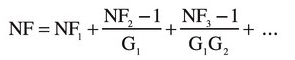
Of course, we get away with weak GNSS signals (most of the time) by replacing antenna gain with receiver-processing gain, thanks to our knowledge of the pseudorandom noise spreading codes used to transmit the signals. Nevertheless, a well-designed antenna is still important for reliable GNSS signal reception (as is a low-noise receiver front end). And as the required receiver position fix accuracy approaches centimeter and even sub-centimeter levels, the demands on the antenna increase, with multipath suppression and phase-center stability becoming important characteristics.
So, how do you find the best antenna for a particular GNSS application, taking into account size, cost, and capability? In this month’s column, we look at the basics of GNSS antennas, introducing the various properties and trade-offs that affect functionality and performance. Armed with this information, you should be better able to interpret antenna specifications and to select the right antenna for your next job.
“Innovation” is a regular column that features discussions about recent advances in GPS technology and its applications as well as the fundamentals of GPS positioning. The column is coordinated by Richard Langley of the Department of Geodesy and Geomatics Engineering at the University of New Brunswick, who welcomes your comments and topic ideas. To contact him, see the “Contributing Editors” section.
The antenna is often given secondary consideration when installing or operating a Global Navigation Satellite Systems (GNSS) receiver. Yet the antenna is crucial to the proper operation of the receiver. This article gives the reader a basic understanding of how a GNSS antenna works and what performance to look for when selecting or specifying a GNSS antenna.
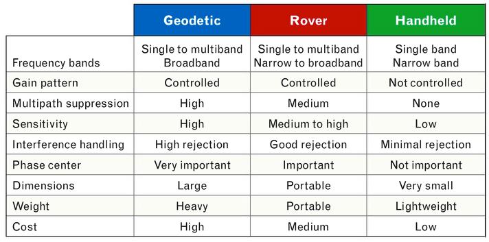
We explain the properties of GNSS antennas in general, and while this discussion is valid for almost any antenna, we focus on the specific requirements for GNSS antennas. And we briefly compare three general types of antennas used in GNSS applications.
When we talk about GNSS antennas, we are typically talking about GPS antennas as GPS has been the navigation system for years, but other systems have been and are being developed. Some of the frequencies used by these other systems are unique, such as Galileo’s E6 band and the GLONASS L1 band, and may not be covered by all antennas. But other than frequency coverage, all GNSS antennas share the same properties.
GNSS Antenna Properties
A number of important properties of GNSS antennas affect functionality and performance, including:
Frequency coverage
Gain pattern
Circular polarization
Multipath suppression
Phase center
Impact on receiver sensitivity
Interference handling
We will briefly discuss each of these properties in turn.
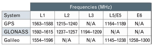
Frequency Coverage. GNSS receivers brought to market today may include frequency bands such as GPS L5, Galileo E5/E6, and the GLONASS bands in addition to the legacy GPS bands, and the antenna feeding a receiver may need to cover some or all of these bands.
TABLE 1 presents an overview of the frequencies used by the various GNSS constellations. Keep in mind that you may see slightly different numbers published elsewhere depending on how the signal bandwidths are defined.
TABLE 1. GNSS Frequency Allocations. (Data: Gerald J. K. Moernaut and Daniel Orban)
As the bandwidth requirement of an antenna increases, the antenna becomes harder to design, and developing an antenna that covers all of these bands and making it compliant with all of the other requirements is a challenge.
If small size is also a requirement, some level of compromise will be needed.
Gain Pattern. For a transmitting antenna, gain is the ratio of the radiation intensity in a given direction to the radiation that would be obtained if the power accepted by the antenna was radiated isotropically. For a receiving antenna, it is the ratio of the power delivered by the antenna in response to a signal arriving from a given direction compared to that delivered by a hypothetical isotropic reference antenna. The spatial variation of an antenna’s gain is referred to as the radiation pattern or the receiving pattern. Actually, under the antenna reciprocity theorem, these patterns are identical for a given antenna and, ignoring losses, can simply be referred to as the gain pattern.
The receiver operates best with only a small difference in power between the signals from the various satellites being tracked and ideally the antenna covers the entire hemisphere above it with no variation in gain. This has to do with potential cross-correlation problems in the receiver and the simple fact that excessive gain roll-off may cause signals from satellites at low elevation angles to drop below the noise floor of the receiver.
On the other hand, optimization for multipath rejection and antenna noise temperature (see below) require some gain roll-off.
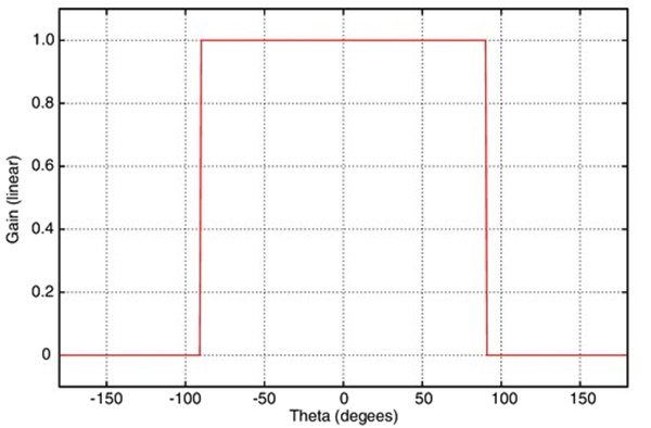
FIGURE 1. Theoretical antenna with hemispherical gain pattern. Boresight corresponds to θ = 0°. (Data: Gerald J. K. Moernaut and Daniel Orban)
FIGURE 1 shows what a perfect hemispherical gain pattern looks like, with a cut through an arbitrary azimuth.
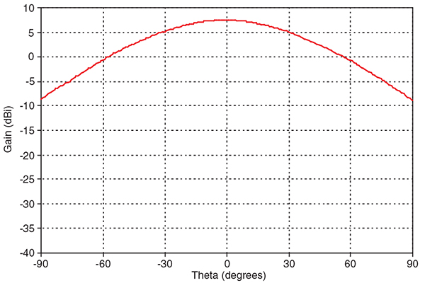
However, such an antenna cannot be built and “real-world” GNSS antennas see a gain roll-off of 10 to 20 dB from boresight (looking straight up from the antenna) to the horizon. FIGURE 2 shows what a typical gain pattern looks like as a cross-section through an arbitrary azimuth.
FIGURE 2. “Real-world” antenna gain pattern. (Data: Gerald J. K. Moernaut and Daniel Orban)
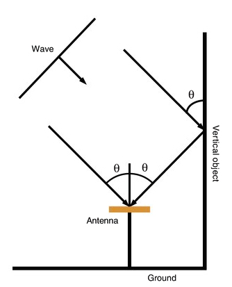
Circular Polarization. Spaceborne systems at L-Band typically use circular polarization (CP) signals for transmitting and receiving. The changing relative orientation of the transmitting and receiving CP antennas as the satellites orbit the Earth does not cause polarization fading as it does with linearly polarized signals and antennas. Furthermore, circular polarization does not suffer from the effects of Faraday rotation caused by the ionosphere. Faraday rotation results in an electromagnetic wave from space arriving at the Earth’s surface with a different polarization angle than it would have if the ionosphere was absent. This leads to signal fading and potentially poor reception of linearly polarized signals.
Circularly polarized signals may either be right-handed or left-handed. GNSS satellites use right-hand circular polarization (RHCP) and therefore a GNSS antenna receiving the direct signals must also be designed for RHCP.
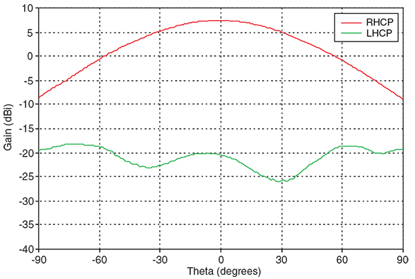
Antennas are not perfect and an RHCP antenna will pick up some left-hand circular polarization (LHCP) energy. Because GPS and other GNSS use RHCP, we refer to the LHCP part as the cross-polar component (see FIGURE 3).
FIGURE 3. Co- and cross-polar gain pattern versus boresight angle of a rover antenna. (Data: Gerald J. K. Moernaut and Daniel Orban)
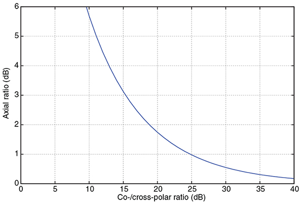
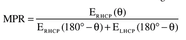
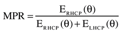
We can describe the quality of the circular polarization by either specifying the ratio of this cross-polar component with respect to the co-polar component (RHCP to LHCP), or by specifying the axial ratio (AR). AR is the measure of the polarization ellipticity of an antenna designed to receive circularly polarized signals. An AR close to 1 (or 0 dB) is best (indicating a good circular polarization) and the relationship between the co-/cross-polar ratio and axial ratio is shown in FIGURE 4.
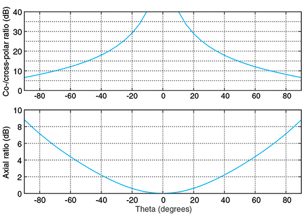
FIGURE 4. Converting axial ratio to co-/cross-polar ratio. (Data: Gerald J. K. Moernaut and Daniel Orban)FIGURE 5. Co-/cross-polar and axial ratios versus boresight angle of a rover-style antenna. (Data: Gerald J. K. Moernaut and Daniel Orban)
FIGURE 5 shows the ratio of the co- and cross-polar components and the axial ratio versus boresight (or depression) angle for a typical GPS antenna. The boresight angle is the complement of the elevation angle.
For high-end GNSS antennas such as choke-ring and other geodetic-quality antennas, the typical AR along the boresight should be not greater than about 1 dB. AR increases towards lower elevation angles and you should look for an AR of less than 3 to 6 dB at a 10° elevation angle for a high-performance antenna. Expect to see small (<1 dB) variations of AR versus azimuth at the low elevation angles.
Maintaining a good AR over the entire hemisphere and at all frequencies requires a lot of surface area in the antenna and can only be accomplished in high-end antennas like base station and rover antennas.
Multipath Suppression. Signals coming from the satellites arrive at the GNSS receiver’s antenna directly from space, but they may also be reflected off the ground, buildings, or other obstacles and arrive at the antenna multiple times and delayed in time. This is termed multipath. It degrades positioning accuracy and should be avoided. High-end receivers are able to suppress multipath to a certain extent, but it is good engineering practice to suppress multipath in the antenna as much as possible.
A multipath signal can come from three basic directions:
The ground and arrive at the back of the antenna.
The ground or an object and arrive at the antenna at a low elevation angle.
An object and arrive at the antenna at a high elevation angle.
Reflected signals typically contain a large LHCP component. The technique to mitigate each of these is different and, as an example, we will describe suppression of multipath signals due to ground and vertical object reflections.
Multipath susceptibility of an antenna can be quantified with respect to the antenna’s gain pattern characteristics by the multipath ratio (MPR). FIGURE 6 sketches the multipath problem due to ground reflections.
FIGURE 6. Quantifying multipath caused by ground reflections. (Data: Gerald J. K. Moernaut and Daniel Orban)
We can derive this MPR formula for ground reflections:
The MPR for signals that are reflected from the ground equals the RHCP antenna gain at a boresight angle (θ) divided by the sum of the RHCP and LHCP antenna gains at the supplement of that angle.
Signals that are reflected from the ground require the antenna to have a good front-to-back ratio if we want to suppress them because an RHCP antenna has by nature an LHCP response in the anti-boresight or backside hemisphere. The front-to-back ratio is nominally the difference in the boresight gain and the gain in the anti-boresight direction. A good front-to-back ratio also minimizes ground-noise pick-up.
Similarly, an MPR formula can be written for signals that reflect against vertical objects. FIGURE 7 sketches this.
FIGURE 7. Quantifying multipath caused by vertical object reflections. (Data: Gerald J. K. Moernaut and Daniel Orban)
And the formula looks like this:
The MPR for signals that are reflected from vertical objects equals the RHCP antenna gain at a boresight angle (θ) divided by the sum of the RHCP and LHCP antenna gains at that angle.
Multipath signals from reflections against vertical objects such as buildings can be suppressed by having a good AR at those elevation angles from which most vertical object multipath signals arrive. This AR requirement is readily visible in the MPR formula considering these reflections are predominantly LHCP, and in this case MPR simply equals the co- to cross-polar ratio.
LHCP reflections that arrive at the antenna at high elevation angles are not a problem because the AR tends to be quite good at these elevation angles and the reflection will be suppressed. LHCP signals arriving at lower elevation angles may pose a problem because the AR of an antenna at low elevation angles is degraded in “real-world” antennas. It makes sense to have some level of gain roll-off towards the lower elevation angles to help suppress multipath signals. However, a good AR is always a must because gain roll-off alone will not do not it.
Phase Center. A position fix in GNSS navigation is relative to the electrical phase center of the antenna. The phase center is the point in space where all the rays appear to emanate from (or converge on) the antenna. Put another way, it is the point where the electromagnetic fields from all incident rays appear to add up in phase. Determining the phase center is important in GNSS applications, particularly when millimeter-positioning resolution is desired.
Ideally, this phase center is a single point in space for all directions at all frequencies. However, a “real-world” antenna will often possess multiple phase center points (for each lobe in the gain pattern, for example) or a phase center that appears “smeared out” as frequency and viewing angle are varied.
The phase-center offset can be represented in three dimensions where the offset is specified for every direction at each frequency band. Alternatively, we can simplify things and average the phase center over all azimuth angles for a given elevation angle and define it over the 10° to 90° elevation-angle range. For most applications even this simplified representation is over-kill, and typically only a vertical and a horizontal phase-center offset are specified for all bands in relation to L1.
For well-designed high-end GNSS antennas, phase center variations in azimuth are small and on the order of a couple of millimeters. The vertical phase offsets are typically 10 millimeters or less. Many high-end antennas have been calibrated, and tables of phase-center offsets for these antennas are available.
Impact on Receiver Sensitivity. The strength of the signals from space is on the order of -130 dBm. We need a really sensitive receiver if we want to be able to pick these up. For the antenna, this translates into the need for a high-performance low noise amplifier (LNA) between the antenna element itself and the receiver.
We can characterize the performance of a particular receiver element by its noise figure (NF), which is the ratio of actual output noise of the element to that which would remain if the element itself did not introduce noise. The total (cascaded) noise figure of a receiver system (a chain of elements or stages) can be calculated using the Friss formula as follows:
The total system NF equals the sum of the NF of the first stage (NF1) plus that of the second stage (NF2) minus 1 divided by the total gain of the previous stage (G1) and so on. So the total NF of the whole system pretty much equals that of the first stage plus any losses ahead of it such as those due to filters.
Expect to see total LNA noise figures in the 3-dB range for high performance GNSS antennas.
The other requirement for the LNA is for it to have sufficient gain to minimize the impact of long and lossy coaxial antenna cables — typically 30 dB should be enough. Keep in mind that it is important to have the right amount of gain for a particular installation. Too much gain may overload the receiver and drive it into non-linear behavior (compression), degrading its performance. Too little, and low-elevation-angle observations will be missed. Receiver manufacturers typically specify the required LNA gain for a given cable run.
Interference Handling. Even though GNSS receivers are good at mitigating some kinds of interference, it is essential to keep unwanted signals out of the receiver as much as possible. Careful design of the antenna can help here, especially by introducing some frequency selectivity against out-of-band interferers. The mechanisms by which in-band an out-of-band interference can create trouble in the LNA and the receiver and the approach to dealing with them are somewhat different.
FIGURE 8. Strong out-of-band interferer and third harmonic in the GPS L1 band. (Data: Gerald J. K. Moernaut and Daniel Orban)
An out-of-band interferer is generally an RF source outside the GNSS frequency bands: cellular base stations, cell phones, broadcast transmitters, radar, etc. When these signals enter the LNA, they can drive the amplifier into its non-linear range and the LNA starts to operate as a multiplier or comb generator. This is shown in FIGURE 8 where a -30-dBm-strong interferer at 525 MHz generates a -78 dBm spurious signal or spur in the GPS L1 band.
Through a similar mechanism, third-order mixing products can be generated whereby a signal is multiplied by two and mixes with another signal. As an example, take an airport where radars are operating at 1275 and 1305 MHz. Both signals double to 2550 and 2610 MHz. These will in turn mix with the fundamentals and generate 1245 and 1335 MHz signals.
Another mechanism is de-sensing: as the interference is amplified further down in the LNA’s stages, its amplitude increases, and at some point the GNSS signals get attenuated because the LNA goes into compression. The same thing may happen down the receiver chain. This effectively reduces the receiver’s sensitivity and, in some cases, reception will be lost completely.
RF filters can reduce out-of-band signals by 10s of decibels and this is sufficient in most cases. Of course, filters add insertion loss and amplitude and phase ripple, all of which we don’t want because these degrade receiver performance.
In-band interferers can be the third-order mixing products we mentioned above or simply an RF source that transmits inside the GNSS bands. If these interferers are relatively weak, the receiver will handle them, but from a certain power level on, there is just not a lot we can do in a conventional commercial receiver.
The LNA should be designed for a high intercept point (IP)–at which non-linear behavior begins–so compression does not occur with strong signals present at its input. On the other hand, there is no requirement for the LNA to be a power amplifier. As an example, let’s say we have a single strong continuous wave interferer in the L1 band that generates -50 dBm at the input of the LNA. A 50 dB, high IP LNA will generate a 0 dBm carrier in the L1 band but the receiver will saturate.
LNAs with a higher IP tend to consume more power and in a portable application with a rover antenna — that may be an issue. In a base-station antenna, on the other hand, low current consumption should not be a requirement since a higher IP is probably more valuable than low power consumption.
GNSS Antenna Types
Here is a short comparison of three types of GNSS antennas: geodetic, rover, and handheld. For detailed specifications of examples of each of these types, see the references in Further Reading.
Geodetic Antennas. High precision, fixed-site GNSS applications require geodetic-class receivers and antennas. These provide the user with the highest possible position accuracy.
As a minimum, typical geodetic antennas cover the GPS L1 and L2 bands. Some also cover the GLONASS frequencies. Coverage of L5 is found in some newer designs as well as coverage of the Galileo frequencies and the L-band frequencies of differential GNSS services.
The use of choke-ring ground planes is typical in geodetic antennas. These allow good gain pattern control, excellent multipath suppression, high front-to-back ratio, and good AR at low elevation angles. Choke rings contribute to a stable phase center. The phase center is documented (as mentioned earlier), and high-end receivers allow the antenna behavior to be taken into account. Combined with a state-of-the-art LNA, these antennas provide the highest possible performance.
Rover Antennas. Rover antennas are typically used in land survey, forestry, construction, and other portable or mobile applications. They provide the user with good accuracy while being optimized for portability. Horizontal phase-center variation versus azimuth should be low because the orientation of the antenna with respect to magnetic north, say, is usually unknown and cannot be corrected for in the receiver. A rover antenna is typically mounted on a handheld pole. Good front-to-back ratio is required to avoid operator-reflection multipath and ground-noise pickup. Yet these rover-type applications are high accuracy and require a good phase-center stability. However, since a choke ring cannot be used because of its size and weight, a higher phase-center variation compared to that of a geodetic antenna is typically inherent to the rover antenna design.
A good AR and a decent gain roll-off at low elevation angles ensures good multipath suppression as heavy choke rings are not an option for this configuration.
Handheld Receiver Antennas. These antennas are single-band L1 structures optimized for size and cost. They are available in a range of implementations, such as surface mount ceramic chip, helical, and patch antenna types. Their radiation patterns are quasi-hemispherical. AR and phase-center performance are a compromise because of their small size. Because of their reduced size, these antennas tend to have a negative gain of about -3 dBi (3 dB less than an ideal isotropic antenna) at boresight. This negative gain is mostly masked by an embedded LNA. The associated elevated noise figure is typically not an issue in handheld applications.
TABLE 2. Characteristics of different GNSS antenna classes. (Data: Gerald J. K. Moernaut and Daniel Orban)
Summary of Antenna Types. TABLE 2 presents a comparison of the most important properties of geodetic, rover, and handheld types of GNSS antennas.
Conclusion
In this article, we have presented an overview of the most important characteristics of GNSS antennas. Several GNSS receiver-antenna classes were discussed based on their typical characteristics, and the resulting specification compromises were outlined. Hopefully, this information will help you select the right antenna for your next GNSS application.
Acknowledgment
An earlier version of this article entitled “Basics of GPS Antennas” appeared in The RF & Microwave Solutions Update, an online publication of RF Globalnet.
GERALD J. K. MOERNAUT holds an M.Sc. degree in electrical engineering. He is a full-time antenna design engineer with Orban Microwave Products, a company that designs and produces RF and microwave subsystems and antennas with offices in Leuven, Belgium, and El Paso, Texas.
DANIEL ORBAN is president and founder of Orban Microwave Products. In addition to managing the company, he has been designing antennas for a number of years.
FURTHER READING
Previous GPS World Articles on GNSS Antennas
“Getting into Pockets and Purses: Antenna Counters Sensitivity Loss in Consumer Devices” by B. Hurte and O. Leisten in GPS World, Vol. 16, No. 11, November 2005, pp. 34-38.
“Characterizing the Behavior of Geodetic GPS Antennas” by B.R. Schupler and T.A. Clark in GPS World, Vol. 12, No. 2, February 2001, pp. 48-55.
“A Primer on GPS Antennas” by R.B. Langley in GPS World, Vol. 9, No. 7, July 1998, pp. 50-54.
“How Different Antennas Affect the GPS Observable” by B.R. Schupler and T.A. Clark in GPS World, Vol. 2, No. 10, November 1991, pp. 32-36.
Introduction to Antennas and Receiver Noise
“GNSS Antennas and Front Ends” in A Software-Defined GPS and Galileo Receiver: A Single-Frequency Approach by K. Borre, D.M.Akos, N. Bertelsen, P. Rinder, and S.H. Jensen, Birkhäuser Boston, Cambridge, Massachusetts, 2007.
The Technician’s Radio Receiver Handbook: Wireless and Telecommunication Technology by J.J. Carr, Newnes Press, Woburn, Massachusetts, 2000.
“GPS Receiver System Noise” by R.B. Langley in GPS World, Vol. 8, No. 6, June 1997, pp. 40-45.
More on GNSS Antenna Types
“The Basics of Patch Antennas” by D. Orban and G.J.K. Moernaut. Available on the Orban Microwave Products website.
Over the past year I’ve attended over a dozen GIS related conferences and sat through over a hundred presentations, most of them PowerPoint. Just like the Dilbert cartoon below I’ve reached my limit of poor PowerPoint presentations and I feel compelled to get on my soap box.
It’s been years since PowerPoint made its entrance but over the past year I still found myself suffering through absolutely horrible presentations. Several years ago there was a Dilbert cartoon in which Dilbert was explaining his side number 397. An audience member, who was actually paying attention, could take it no more and with a scream passed out. Wally, who had been sleeping, examined him and declared “PowerPoint Poisoning!” This may be funny but it strikes too close to reality.
Over the past year, I’ve attended more than a dozen GIS-related conferences and watched at least a hundred presentations, most of which were conducted in Microsoft PowerPoint. It’s been years since this now-ubiquitous software made its entrance, yet I still find myself suffering through absolutely horrible presentations. PowerPoint has made slide creation so easy that neurotic presenters with no skills, no taste, and no judgment are free to make us squirm in our seats. I’ve finally reached my limit, and I feel compelled to get on my soapbox.
First, a little history from an old guy who did presentations in the early eighties the hard way: with a grease pencil on overhead projector glass. In the late eighties I was lucky enough to be at a command where the graphics department could create professional-looking transparencies or 35-millimeter slides. The slides looked good, but because of the cost and hassle involved, presenters thought through their points carefully and used the slides sparingly.
In the early nineties, Harvard Graphics and PowerPoint hit the streets along with LCD projectors, and what should have been a wonderful tool quickly became a curse to many. Edward Tufte, the well-known author and Yale professor of information design, railed against PowerPoint. He used the famous 1869 graphic by Charles Joseph Minard of Napoleon’s march to Moscow as a superb example of the right way to communicate data graphically. This graph is still considered the single best example of elegant simplicity in using a map to display spatial and temporal data.
Charles Joseph Minard created this “figurative map” of Napoleon’s march to Moscow. The image shows the route of the army’s march, the temperature, and personnel attrition over time. The brown band represents the men who enter into Russia, and the black band represents those who leave it.
That’s how it was done in olden times: slow, deliberate, and thoroughly thought out. PowerPoint has facilitated the exact opposite behavior, with legions of presenters using the high-tech tool as a toy. I remember sitting thorough a presentation given by a senior executive of a major power company in Georgia. It was about a year after Microsoft added sound effects and the bullet fly-in feature to PowerPoint, and this presenter had each bullet fly in with a unique animation and sound effect. After a few minutes, no one was paying attention to the content; the audience chuckled and murmured, trying to predict which effect would come next. The only thing that presenter was missing was a big red nose and floppy shoes.
Worth a Thousand Words
In the GIS community, we are especially lucky, because most of our content is a graphic representation of spatial data. I think that’s what attracted me to GIS — its graphic visual nature. In GIS classes I’ve taught, I frequently pointed to a universal human characteristic: our learning, memory, and perception are very much graphically oriented. As an example, I cited the work of scientists who determined that the average person has almost 200,000 discrete human faces in their mental database. That’s pretty amazing, considering the relatively minor differences between faces; we have such discerning powers of observation that even Hollywood impersonators can’t fool most viewers. Of the thousands of Elvis impersonators, many come close to the real thing, but I have yet to see one that’s spot-on.
So I encourage people to take advantage of that human trait and use graphs, maps, imagery, and photos — not text — as visuals in their communication. Most PowerPoint trainers recommend using very little text, and limiting a presentation to no more than 35 slides and no more that 25 words on any given slide. They also caution to never, ever read the slides aloud. The slides are supposed to enhance the presenter’s presentation, not replace the presenter. My feeling about any presenter that reads his slides aloud is: Save yourself the trip! Stay home and just e-mail me your PowerPoint.
Good Tools, Bad Results
One problem with computers is that anyone can produce content that is technically perfect, such as documents, maps, or slides. But technically nice lines and fonts don’t guarantee a good-looking or effective end result. I learned that when I was the GIS Manager for the Atlanta Regional Commission (ARC). In the mid-nineties we started publishing our GIS data on CD so our ARC users could create their own maps. The results were some of the worst maps I’ve ever seen. We quickly learned that when wielded by someone with no cartographic or artistic skills, even sophisticated GIS tools could result in horrid presentations.
The same held true for Internet projects. In the early years of the Web, the new technology was difficult to master quickly, so we hired a computer firm specializing in Web site creation. I remember asking the company owner about the challenge of finding good HTML programmers. He surprised me with his answer: it was relatively easy to find programmers, but he couldn’t teach them how to be artists and create content that looked good. He said it was easier to start by hiring good artists, and then teach them the programming skills needed to create Web sites.
And that’s the problem with PowerPoint: Learning the software doesn’t guarantee good presentations. In addition to knowledge of the software, good presentations require artistic talent, a command of the material, and exceptionally good judgment as to how to communicate with your audience.
I think that many people who overdo PowerPoint do it out of insecurity; they want to show everyone how complicated their job is, and how much stuff they handle. While I was at ARC, I tried countless times to convince our planners that more is less. Frequently they would conduct slide shows containing 80 to 90 slides, with many slides containing more than 100 words each. When these “planning shows” were scheduled, you could see the look of dread on the faces of our board members. The old “I just got a silent-ring cell phone call and I have to leave the room” trick was used frequently.
Trimming the Fat
Thankfully, some of these problems have been partially addressed. Good-looking, interactive GIS maps can now be created using ESRI’s MapPublisher, TerraGo’s GeoPDF, or some of the Adobe PDF map formats. All permit the preservation of color schemes, fonts, line widths, symbology, and other cartographic elements in the interactive environments.
Many companies and conference organizers try to improve the artistic aspect of PowerPoint presentations by requiring presenters to use a standard conference template. But that only standardizes the look, without affecting the content or the way it’s delivered. Now, there’s finally hope that tediously long presentations may get reined in as well.
There is a relatively new trend you’ve probably heard of called Pecha Kucha (Japanese for “chitchat”). Many pronounce it the way it looks, although the proper pronunciation is “peh chach ka.” This patented presentation method was started by architects Mark Dytham and Astrid Klein. While working in Japan, they would hold shows for young designers. Since they wanted to give many designers the opportunity to show their work, they developed a fast-paced format that limited each presenter to 20 slides and only 20 seconds per slide. The end result was a short presentation: just six minutes and forty seconds.
Think about the ramifications of this. Just like a “thirty-second elevator pitch,” presenters had to really think through their presentations and distill their material down to only the key points. Currently, most conferences give presenters twenty minutes, plus another five to ten minutes for questions. With a seven-minute limit per session, there can be more time for questions, or for more presentations. The trend is spreading like wildfire: Autodesk is hosting Pecha Kucha nights during conferences, and Bentley and some universities are doing the same. ESRI has tested the format at some local conferences, and the 2009 Annual URISA Conference will have a Pecha Kucha night that I’m looking forward to participating in. My current PowerPoints have fewer than thirty-five slides, and fewer than forty words total, but I’m working to whittle that number down to twenty.
If you want to learn more, check Google or YouTube, which have many examples to choose from. I promised myself that every time I’m subjected to a poor PowerPoint presentation, I’m going to give the presenter a copy of this article. Maybe you could do the same, and we can collectively raise the bar and see fewer bad presentations in the coming year.
Well, it’s time to get off the soapbox. So, if you aren’t neurotic, and you’re confident with your knowledge and position, try giving your audience more by giving them less — adopt Pecha Kucha and help cure PowerPoint Poisoning.
GMV, a supplier of satellite ground system software headquartered in Madrid,
Spain, with a significant role in Europe’s Galileo program, has announced
the appointment of Jesus Serrano as its new Chief Executive Officer (CEO).
Serrano, 48, replaces Luis Mayo in his position as the business group’s top
executive, reporting directly to the board.
With more than 20 years of experience through various management positions
at GMV, this Spanish native will continue to lead the multinational technology
group and expand their products and services to its customers throughout the
U.S., South America, Africa, Asia and Oceania.
The U.S. International Trade Commission (ITC) has issued an exclusion order against certain SiRF GPS chips and products containing those chips imported into the United States, as well as cease-and-desist orders against SiRF and four specific SiRF customers.
This comes after the commission affirmed an ITC administrative law judge’s initial determination that SiRF infringes on three additional GPS patents held by Global Locate Inc., a wholly owned subsidiary of Broadcom. This latest ruling brings the total number of Global Locate GPS-related patents that SiRF has been found to infringe up to six.
In 2008, an ITC administrative law judge found that SiRF infringed on all six patents asserted by Global Locate/Broadcom and subsequently recommended an import ban within in the United States; SiRF appealed the finding. The full ITC Commission subsequently upheld the administrative law judge’s finding on three patents, while holding off on a final determination on the other three pending further review. On Thursday, January 15, the commission issued both its Final Determination on those patent issues and orders regarding the appropriate form of remedy.
“We are optimistic that the ITC orders will become effective after a 60-day statutory review period so that U.S. Customs may begin enforcement and prevent any further patent infringement,” said David Rosmann, Broadcom’s vice president for intellectual property litigation.
The six patents at the center of the dispute are United States patents 6,417,801; 6,937,187; 6,606,346; 7,158,080; 6,704,651; and 6,651,000 — relating to extended ephemeris assistance, calculating time in GPS receivers, enhancing sensitivity in assisted GPS systems, and implementing hardware structures for parallel correlation, according to Broadcom. These patents involve several SiRF products, including SiRFstarIII and SiRFInstant devices.
For its part, however, SiRF said that the impact of the ITC’s decision is minimal, as the products involved are legacy products. It also hinted that it could still file an appeal in federal court.
“We are pleased that the commission followed the Federal Circuit’s Kyocera ruling, which significantly limits the impact to our customer base,” said Kanwar Chadha, founder of SiRF in a statement. “While disappointed with the commission’s ruling as it relates to its patent infringement findings regarding SiRF’s earlier products, we continue to work closely with the named customers to conform with the commission’s ruling and enable them to maintain uninterrupted product delivery to market.”
Chadha was referring to a federal circuit court’s October 14, 2008, decision that ITC limited exclusion orders only affect parties named in an investigation involving Kyocera. Other than the four named customers in the investigation, all other SiRF customers are not affected, the company said. Those four customers have not been named publicly.
SiRF further noted that following the 60-day presidential review period it has the option to appeal the case to the U.S. Court of Appeals for the Federal Circuit, but did not specifically say it would pursue this option. Broadcom and SiRF are already duking it out in federal district court over patent disputes; that trial is scheduled to begin in November 2010.


 Chadha Says. “From a strategy viewpoint,” SiRF founder and vice president of marketing Kanwar Chadha told GPS World, “multi-function radios is something we have been talking about for two years. Market opportunities became much larger in the last six months, with Nokia driving loction into every mobile phone.
 Epson, Infineon Develop Tiny Single-Chip Receiver
 u-blox Launches Cards for Mobile Computers