Consumer-Grade GPS Receivers for GIS Data Collection
I hereby proclaim June GPS/GIS month (at least for me). I’m dedicating the next three newsletter columns (early June, mid-June, and early July) and a webinar (June 30) to discussing using GPS receivers and technology for GIS (geographic information systems) data collection. Why, you may ask?
First of all, I realize my domain is typically the high-precision survey/construction arena, but the boundary isn’t so clear cut any longer. Many surveyors, engineers and construction crews use less accurate GPS receivers for activities such as GIS data collection, recon, and navigating — so the topic is relevant.
Secondly, ’tis the season. The ESRI User Conference is in mid-July this year — about six weeks from now. Although high-precision GPS has a firm place there and is growing, the ESRI UC is the largest conference in the world where non-survey GPS is near center stage. It is one of the primary data-gathering tools that fuels a GIS.
There have been some really significant changes in the last 10 years. GPS data-collection tools for GIS have expanded. At that time, consumer receivers couldn’t be used because Selective Availability (SA), the intentional degradation of GPS accuracy by the Department of Defense, was still active. Also, “submeter” GPS mapping systems were backpack-based, contained a “rat’s nest” of cables, required camcorder batteries to run, and were generally bulky. Data collectors were based on DOS instead of Windows. Lastly, users were primarily using post-processing to differentially correct their GPS data or using Marine DGPS/NDGPS in select locations or commercial DGPS services like OmniSTAR for real-time DGPS.
Fast forward to today. Three categories of GPS are being used to populate GIS databases: consumer-grade receivers, GPS receivers designed specifically for GIS data collection, and survey receivers used for GIS data collection. In this column, I’ll discuss using consumer-grade receivers for GIS data collection. In my mid-June column, I’ll discuss the class of GPS receivers designed specifically for GIS data collection.
Consumer-Grade Receivers
Overnight, when SA was turned off in May 2000, consumer-grade GPS receivers became a viable option for GIS data collection where accuracy is not of the highest priority. Today, due to improvements to the GPS itself as well as GPS receiver technology and along with the maturation of WAAS/SBAS, consumer-grade GPS accuracy is even better.
Thousands, maybe tens of thousands, of consumer-grade GPS receivers are being used to collect data used for GIS. They are easy to use and the price is attractive.
Understanding the accuracy of a consumer-grade GPS receiver is not a simple task. In fact, if you’re not careful, you can be easily misled. For example, take a receiver out to the parking lot and wait for it to obtain enough satellites and a WAAS/SBAS correction. You may be impressed with its precision as it might be within a couple of meters or even better. There are two issues with this:
Repeatability…accuracy vs. precision. Precision is a group of points that are tightly clustered but not in the right place. For example, you may have a cluster of 10 points all within two meters of each other, but they are five meters from the true location. This is not necessarily desirable, but quite typical for consumer-grade GPS receivers. Some receivers offer an “EPE” (Estimated Positional Error) value on the display to provide you and indication of accuracy. Absolutely do not rely on this value in an attempt to estimate the position accuracy of the receiver. It is a rough guess at best.
Performance in less-than-desirable GPS conditions. Surprisingly, or not, users assume that performance in a grove of trees is going to be similar to performance in a parking lot with a wide open view of the sky. This is not the case.
I’ll give you a real case study. Several years ago I was helping a company setup a GPS system to map utility poles. Their required accuracy was +/- 3 meters. A local survey equipment salesperson suggested they use a consumer-grade Compact Flash (CF) GPS receiver plugged into the top of a ruggedized PDA. The salesperson demonstrated the receiver in the client’s parking lot. The performance, in the client’s eyes, seemed like it would meet the +/- 3 meter requirement. The price was right at $250 per receiver and they need upwards of 15 receivers. There were a couple of alternative proposals that cost significantly higher per receiver ($2,000-$4,500 each). The price difference was too great for the client not to be tempted to try the $250 receiver so they purchased six of them. They ended up using them for only 60 days. The bottom line was that the receiver performed very poorly in the field in two areas. First, many of the utility poles were located in areas where there were many trees. The client found that the CF GPS receiver performed very poorly in that environment. Some positions were off by more than 50 meters. Secondly, the client found that the CF GPS receiver had a difficult time maintaining lock on the WAAS satellites used for corrections even in relatively wide open areas where this shouldn’t have been a problem.
In this case, the lesson is to try the receiver in an environment where you will be using it. All GPS receivers will perform worse under tree canopy as compared to their performance in an open area. This is the Achilles heel of GPS. That being said, some GPS receivers perform better under tree canopy than others. The ones that do perform better under trees were designed to do so. Using a consumer-grade GPS in that environment is sort of like trying to compete in a Formula One race with a Volkswagen Beetle. The design criteria of the Beetle was fuel economy and low cost, not acceleration and cornering. The same applies to consumer GPS receivers. Accuracy is not one of the top criteria for consumer GPS receiver designers. They are much more concerned with low cost, low power consumption, small antenna size and fast satellite acquisition, as they should be. My wife, for example, really doesn’t care if it’s accurate to 15 meters vs. 1 meter as long as she arrives at the destination she plugs into the system. On the other hand, high-performance GPS receivers designed for GIS data collection sacrifice some features such as power consumption, antenna size, and small size in order to optimize accuracy.
This is not to say that consumer GPS receivers have no place in GIS mapping. On the contrary, they have a very important place. My point is that your expectations should match reality when evaluating receivers to use for your project. The accuracy specifications on consumer GPS receiver datasheets are essentially meaningless. The only way to truly understand the performance of a particular receiver is to try it yourself.
One final note on this. Many commercial (typically survey equipment dealers) and academic entities have published accuracy comparisons of different consumer GPS receivers. You really have to take these reports with a grain of salt. Sometimes the reports are intentionally biased and other times they are biased due to lack of knowledge or experience. They are also based on an environment that may not be similar to yours. “Heavy” tree canopy is a subjective term. Tree canopy in Oregon is different than tree canopy in Alberta and is different from tree canopy in Austria.
The Final Analysis
Upside:
Low cost
low power
user-friendly
small
Downside:
Poor accuracy in challenging GPS conditions
inconsistent accuracy in non-challenging GPS conditions
A Preliminary Analysis of SVN49’s Demonstration Signal
By Michael Meurer, Stefan Erker, Steffen Thölert, Oliver Montenbruck, André Hauschild, and Richard B. Langley
Great excitement surrounds the activation of a new transmitter from a satellite — an occasion dubbed first light. Research groups around the globe joined the GPS Wing in monitoring and analyzing the first L5 signals from space. We describe the equipment and procedures used to capture and analyze SVN49’s signals and give an assessment of their characteristics.
INNOVATION INSIGHTS by Richard Langley
ON APRIL 10, a new type of radio signal was transmitted from space. I am referring, of course, to the L5 demonstration signal from the Block IIR-M satellite SVN49, launched on March 24. The L5 signal, the second of two new civil GPS signals, will be standard on the next generation of GPS satellites — the Block IIFs — and its frequency band was duly registered with the International Telecommunication Union (ITU) back in 2002. But satellite operators only have seven years after filing a frequency application to start transmitting signals from the designated orbit, and delays in launching the first Block IIF satellite meant that GPS could lose the allocation. The GPS Wing and its contractors determined that the best way to secure the L5 frequency was to add an L5 demonstration payload to one of the remaining modernized Block IIR satellites. And so SVN49 made history with the inaugural broadcast of L5 with just a few months to spare before the clock ran out on the ITU filing.
Great excitement always surrounds the first photons captured by a new telescope or other detectors of electromagnetic signals. Or when a transmitter is activated for the first time. Just as we do for the dawning of a new day, we call this occasion first light. Research groups around the globe joined the GPS Wing in monitoring and analyzing the first L5 signals from space, including a group of scientists and engineers from Germany and Canada. This month the group describes the equipment and procedures used to capture and analyze SVN49’s signals and gives an assessment of their characteristics.
“Innovation” features discussions about advances in GPS technology and applications as well as fundamentals of GPS positioning. The column is coordinated by Richard Langley of the Department of Geodesy and Geomatics Engineering, University of New Brunswick. To contact him, see “Contributing Editors.”
A key feature of GPS modernization is the addition of the L5 civil signal to the suite of signals transmitted by the satellites. The introduction of such a signal on a different carrier frequency than that used by the legacy L1 GPS signal was proposed in the 1995 reports by the U.S. National Research Council and the National Academy of Public Administration on the future of GPS. The reports argued that an unencrypted signal on a second frequency would offer civil users the benefit of ionospheric delay correction, wide-lane carrier-phase ambiguity resolution, improved interference rejection, and faster accuracy recovery in multipath environments.
Studies showed that it would be possible to add a civil signal on the L2 frequency without compromising the military signal. High-precision (and accuracy) civil users had been using the L2 frequency — initially designated for military use only — ever since the first GPS satellites were launched, and through clever (though suboptimum) tracking techniques even after the L2 signals were encrypted. An unencrypted signal on L2 would bring these users a more robust signal as well as affording all civil users the benefits of a second frequency. But unlike the L1 signal, the L2 signal is situated in a part of the radio spectrum not officially protected from interference by other users of the spectrum. So such a second civil signal could not be used for safety-of-life applications such as navigating aircraft.
So, in Vice President Al Gore’s statement of March 30, 1998, on the enhancement of GPS for civil users, the decision to deploy two new civil signals was announced: the civil signal on L2, now known as L2C, and a signal on a new frequency, which became known as L5. Some readers might wonder why this new signal was not designated L3 or L4. Those designations had already been assigned to signals associated with other payloads on the GPS satellites.
Although the Gore announcement proposed to introduce both of the new civil signals with the launch of the Block IIF satellites, the addition of the L2C signal to the legacy signals was deemed a relatively straightforward task and the decision was made to modify the last eight Block IIR satellites for the provision of L2C. The first modernized Block IIR satellite was launched on September 26, 2005, and seven of these satellites are now in orbit.
The frequency selected for the L5 signal, 1176.45 MHz, is in a protected aeronautical radionavigation services (ARNS) band. This frequency, as with frequencies used by all satellite operators, had to be coordinated with the International Telecommunication Union-Radiocommunication Sector (ITU-R). The ITU-R registers frequencies essentially on a first-come, first-served basis, but a user must actually transmit signals on the assigned frequency from the designated satellite orbit type within seven years from the date of filing with ITU-R. This meant that L5 signals had to be transmitted before August 26, 2009, to avoid the potential claim of the frequency by a different country. A decision was made to modify an existing Block IIR-M satellite to carry an L5 demonstration payload. The L5 demo payload, which was developed by Lockheed Martin and its subcontractors, was added to space vehicle number (SVN) 49. SVN49 was launched on March 24, 2009, the seventh modernized Block IIR satellite to be placed in orbit. Also known as PRN1, from the primary pseudorandom noise (PRN) codes assigned to the satellite, the satellite began L5 transmissions on April 10, at 11:58 UTC, and so satisfied the ITU-R filing requirement with a few months to spare.
The L5 Signal Structure
The structure of the future full L5 signal will differ significantly from the legacy L1 signal or even the modernized L2C signal. It is fully described in the Navstar GPS L5 interface document, IS-GPS-705. We present just a brief overview of the signal here.
Two-Component Signal. The full L5 signal will offer two signal components: one with and one without a superimposed navigation data message. The two signal components — in-phase (I) and quadrature (Q) — have equal power. Both will have a minimum received power of –157 dBW. Each component is modulated with a different, but synchronized, L5 PRN code. The in-phase component (the I- or data channel) is further modulated with a 100-symbol per second (sps) symbol stream carrying the navigation message data, and the quadrature component (the Q- or data-free channel, also called the pilot channel) is modulated only with a PRN code. Different, nearly orthogonal PRN codes (referred to as I5 and Q5) are used in the two components to prevent tracking biases by making each component completely independent of the other, except for the underlying carrier phase.
Another novel aspect of the L5 signal design is the use of Neuman-Hoffman (NH) synchronization codes.
Code Structure. As previously mentioned, the I5 and Q5 channels are modulated with different PRN codes. These codes differ significantly from the C/A-, P-, and L2C-codes used on L1 and L2 both in length and chipping rate.
The natural code chipping-rate frequency of 10.23 MHz as provided by the SV atomic frequency standards satisfies a number of requirements for a modernized signal within the bandwidth constraints — increased bandwidth efficiency, improved signal accuracy, immunity to waveform distortion, and improved rejection of narrowband interference. The bandwidth constraints include rejection of out-of-band interference. Accordingly, a 10.23 megachip per second (Mcps) chipping rate, 10 times that of the C/A- and L2C-codes, was adopted for the L5 PRN codes.
Improved Cross-Correlation. There is a trade off between code period and the capability to do direct acquisition. A longer code period provides better cross-correlation properties, but takes longer to search. However, one can speed up an acquisition to some extent with lower code cross-correlation levels.
The L1 C/A-code period is 1023 chips, or 1 millisecond. The desire to maintain that epoch rate of 1 kHz with the 10.23 Mcps chipping rate results in a code period of 10,230 chips. For both the I5 and Q5 ranging codes, the 1-millisecond sequences are the modulo-2 sum of two sub-sequences referred to as XA and XB with lengths of 8,190 and 8,191 chips, respectively. The same XA sequence is used for both I5 and IQ, whereas the XB sequence for I5 is different from that for Q5. The XB sequences are selectively advanced to produce different 1-millisecond-long code sequences. In this way, a large number of unique codes can be generated. Thirty-seven primary code pairs have been designated, of which 32 are reserved for use by GPS satellites (PRNs 1–32). An additional 173 pairs have been defined (PRNs 38–210). PRN sequences 38 through 63 are reserved for satellites.
Demo Signal Verification
The L5 signal transmitted by SVN49 contains only the dataless quadrature component modulated with the PRN63 Q5 sequence. Furthermore, the transmitted L5 signal power and the satellite antenna radiation pattern are different from those expected for the L5 signals to be transmitted by the Block IIF satellites as described in the L5 interface specification.
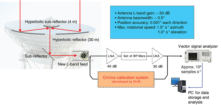
Over the past few weeks, the German Aerospace Center (Deutsches Zentrum für Luft- und Raumfahrt or DLR) has monitored SVN49 using its GNSS verification and analysis facility. The core element of the facility is a 30-meter dish antenna at Weilheim, near Munich, Germany, and is shown in FIGURE 1. The antenna, which is based on a shaped Cassegrain system, has a 30-meter-diameter parabolic reflector and a hyperbolic sub-reflector with a diameter of 4 meters. The L-Band gain of this high-gain antenna is around 50 dB, with a beam width of less than 0.5°. The position accuracy in both azimuth and elevation directions is 0.001°. The antenna’s maximum slewing speeds are 1.5° per second in azimuth and 1.0° per second in elevation angle, allowing it to easily track MEO satellites.
FIGURE 1. GNSS verification and analysis facility with 30-meter high-gain antenna at Weilheim, Germany.
In September 2005, DLR’s Institute of Communications and Navigation established an independent monitoring station for the analysis of GNSS signals using this powerful instrument. For the new challenge, the antenna was adapted to the requirements in the navigation field. A newly developed broadband circularly polarized feed and a new receiving chain including an online calibration system were installed at the antenna during preparations for the GIOVE-B in-orbit test campaign in the spring of 2008.
During this time, intensive work on the system calibration was performed using well-known signals from radio “stars” and EGNOS satellites for the antenna gain determination, and sophisticated calibration methods for the receiving system. The calibration provides an absolute measurement uncertainty significantly less than 1 dB.
Due to the distance of the antenna location from the institute at Oberpfaffenhofen (around 40 kilometers), it was necessary to perform all measurement and calibration procedures during the measurement campaigns under remote control. A software tool was developed that can control any component of the setup remotely. In addition, this tool is able to perform a completely autonomous operation of the whole system by a pre-definable sequence over any period of time. Additional details about the GNSS verification and analysis facility and the calibration techniques used can be found in the literature cited in Further Reading.
A detailed signal-in-space (SIS) analysis of the new L5 signal transmitted by SVN49 was conducted by recording several passes with the GNSS verification and analysis facility. A high elevation-angle transit of SVN49 every night allows a long observation time for each satellite pass. To ensure precise tracking of the satellite with the high-gain antenna, we used the latest two-line element sets from the U.S. Air Force Space Command.
The first signals transmitted by the satellite on the L5 frequency were captured during the pass on April 10. Compared to later measurements, the power of the L5 payload signal was measured with a lower output level on this first pass. This points to a power “fade in,” which is a common procedure in commissioning a new satellite payload. A controlled and slow heating of the payload elements avoids possible damage caused by the out-gassing of the power amplifiers, for example.
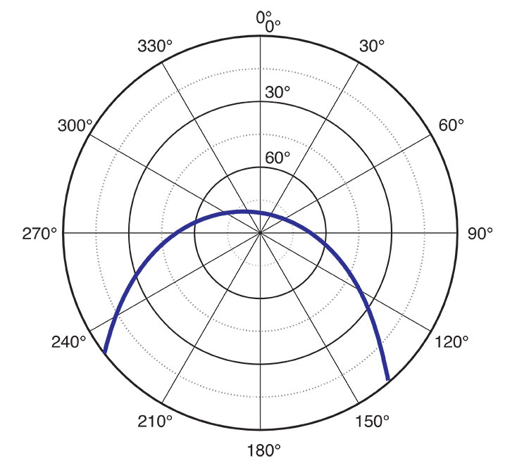
The SIS analyses that we performed using the high-gain antenna will be described for one example satellite pass recorded on April 29. During this pass, the satellite reached an elevation angle of around 80° and was visible for about seven hours (see FIGURE 2). A set of spectral snapshots as well as time sample records for the L1, L2, and L5 signals were processed and adjusted with the corresponding calibration values during a post-processing stage.
FIGURE 2. Skyplot of SVN49 pass at Weilheim, Germany, on April 29, 2009.
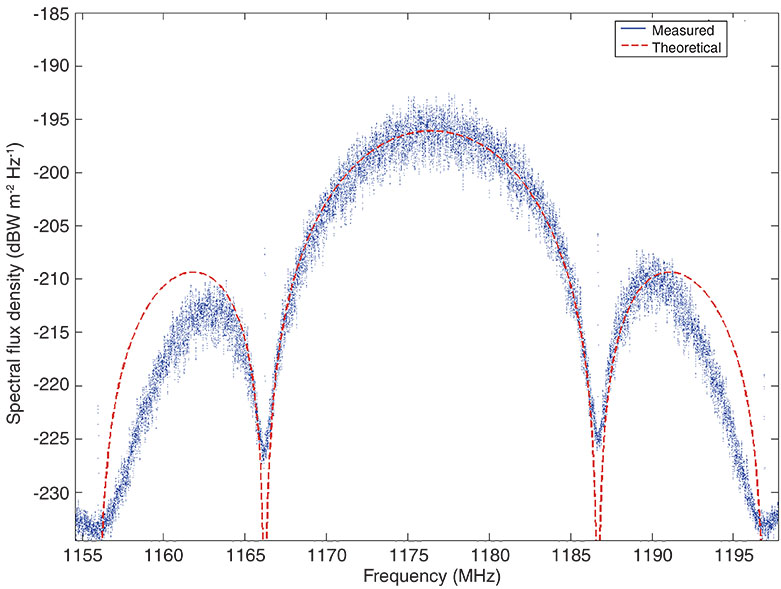
Time and Frequency. A first view of the captured spectrum snapshot in FIGURE 3 shows the L5 signal and its typical binary phase-shift-keyed (BPSK) spectral shape. The signal is significantly band limited by the used front-end filters of the satellite’s L5 payload. This ensures the required spectral separation from the adjacent L2 signal of the satellite, as the L5 signal must not interfere with the operational L2 frequency. Overlaying the theoretical spectral mask of the L5 BPSK signal, we note a slight asymmetry of the spectral shape. The two side lobes differ around 2.5 dB in their peak power level (see Figure 3). Spectral asymmetries of that kind typically result from frequency selectivity in the RF transmitter chains in satellite payloads, including the amplifiers and antennas.
FIGURE 3. L5 spectrum plot from data recorded on April 29.
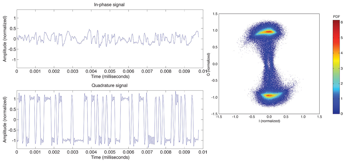
FIGURE 4 shows a temporal snapshot of the L5 signal after wiping off the Doppler frequency shift due to satellite orbital motion. Figure 4 (left) depicts a snapshot of 10 microseconds for the I and Q channels. It can be seen, that in compliance with the requirements of the L5 signal explained in the introduction of this article, the signal is a bi-level signal with a chipping rate of 10.23 Mcps. Plotting the normalized histogram of the L5 signal, one obtains the normalized I/Q probability density function (PDF) diagram of the L5 signal shown in Figure 4 (right). The constellation diagram shows a remaining deformation of the Q component after Doppler removal. Although the L5 signal transmitted by the test payload only contains the dataless Q5 component, a non-negligible contribution can be seen in the I channel. This slight distortion may stem from a nonlinear and frequency-dependent amplification of the Q baseband signal leading to crosstalk between the Q and I channels.
FIGURE 4. (left) L5 I and Q time samples; (right) L5 I/Q probability density function (PDF).
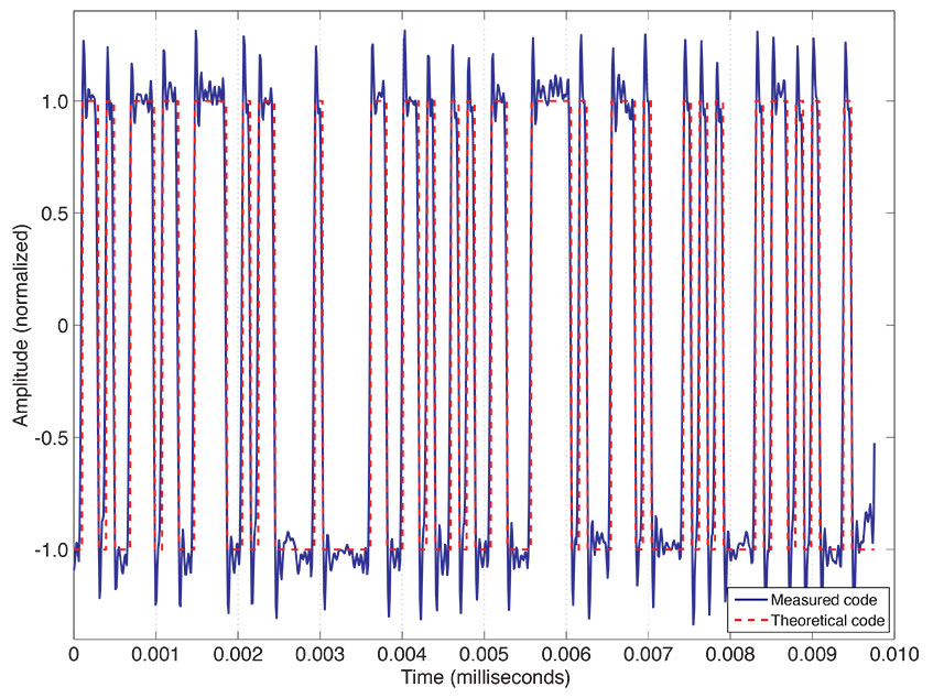
Signal Code Sequence. With the use of the high-gain antenna, it is possible to look in detail at the transmitted L5 code chips. The signal is raised high above the noise floor and, after Doppler wipe off, allows us to compare the received code sequence with the theoretical code sequence for the PRN63 Q channel. FIGURE 5 shows an example for the first 10 microseconds of the code — both for the measured L5 signal and the expected theoretical code. The analysis performed also for several full code periods shows that the demo payload’s Q5 code structure is in full compliance with the “theoretical” code described in the official signal interface document.
FIGURE 5. Comparison of measured and theoretical code sequences.
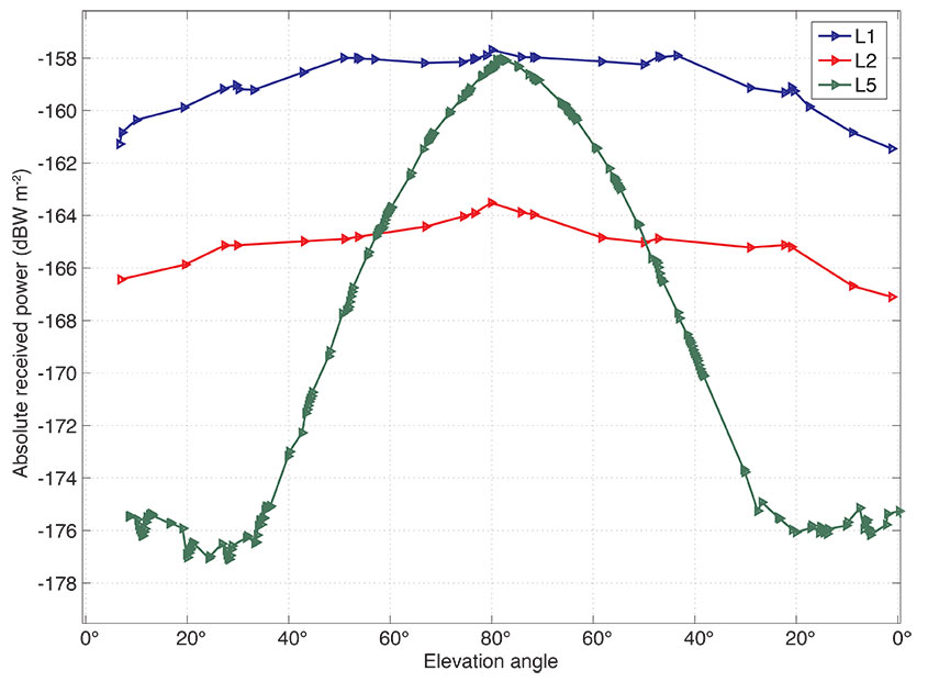
Power of Received Signals. The GNSS verification and analysis facility is fully calibrated, allowing highly accurate absolute measurements of GNSS signal power levels. We have used the system to evaluate the SVN49 signal power levels as received on the ground. FIGURE 6 shows the different signals transmitted in the L1, L2, and L5 frequency bands in terms of the received power per square meter versus elevation angle of the SV during its pass. It can be seen that there is a significant elevation-angle dependency of the L5 received power (about 18 dB between low and high elevation angles) compared to L1 and L2 (with a variation of about 3 dB). In this measurement, the combined power of the I and Q channels is plotted for the signals. So this means that the L1 and L2 signal measurements include the power of the C/A-, P(Y)-, and M-codes. Such a strong elevation-angle dependency is not typical of signals radiated by GPS satellites. However, the L5 signal is radiated using the legacy L1/L2 Block IIR-M satellite antenna, which is to the authors’ knowledge not optimized for the L5 frequency.
FIGURE 6. Absolute received power for SVN49 L1, L2, and L5 signals on April 29, 2009.
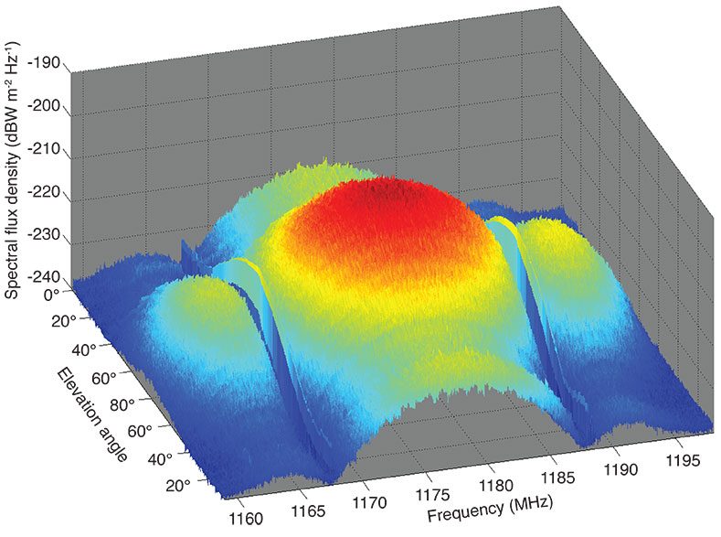
In the spectrogram plot of FIGURE 7, which was generated by plotting all recorded L5 spectra versus elevation angle, the impact of this elevation-angle dependency of the received power can be detailed for the complete frequency range. The side lobes of the BPSK signal are only clearly visible in the spectrogram at higher elevation angles.
FIGURE 7. Spectrogram for L5 signal received on April 29, 2009.
Signal Tracking
In parallel with the detailed signal validation using the high-gain antenna and vector signal analyzer, an effort has also been made to track the new GPS L5 signal using conventional correlating GNSS receivers. Given the relevance of L5/E5 signals for future aeronautical applications and the ongoing transmission of such signals from the GIOVE satellites, a growing number of commercial receiver manufacturers have announced receivers supporting this frequency band. However, due to the special nature of the SVN49 test signal (pilot only, with different PRN code designations on L1 and L5) some modifications to receiver software are required to properly track the first GPS L5 signal. In particular, the use of different PRN code designations employed for L1/L2 (PRN1) and L5 (PRN63) is clearly non-standard and requires suitably adapted receiver software, which was provided by the makers of the two receiver types we selected for our test campaign.
Receiver type N is a highly configurable test receiver for L1 and L5/E5a signals developed as part of the Galileo program. It offers a total of 16 tracking channels, which are implemented in a field-programmable gate array and can thus be flexibly adapted for tracking of civil GPS, satellite-based augmentation systems, and the GIOVE-A and -B signals in their respective frequency bands. Receiver type J, in contrast, represents the latest generation of geodetic grade multi-constellation receivers. It uses an advanced application-specific integrated circuit with 216 tracking channels supporting all types of non-military navigation signals in the L1/E1, L2, and L5/E5a bands. Both receivers have been used for some time prior to the launch of SVN49 to track GPS and GIOVE satellites from stations at the University of New Brunswick (UNB) in Canada and at DLR in Germany.
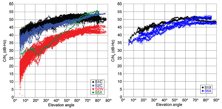
The first measurements of GPS L5 were successfully collected on April 10 with a type N receiver at UNB. While these measurements confirmed the capability to properly track SVN49 in the L5 band, they already revealed a distinct aspect of the GPS L5 test signal that potential users must be aware of. The signal is much weaker at low elevation angles than the L1 signal. Normal carrier-to-noise-density ratios (C/N0) are only achieved at elevation angles of about 60° and higher. On the other hand, the measured C/N0 near zenith may even outperform that of L1 and L2 tracking with sufficient L5 antenna gain. For illustration, FIGURE 8 compares the measured C/N0 values of GPS and GIOVE-A/B signals as obtained with receiver type J and a geodetic antenna at DLR, Oberpfaffenhofen.
FIGURE 8. Comparison of the relative signals strength (expressed as carrier-to-noise-density ratio, C/N0) for GPS (left) and GIOVE-A/B signals (right). The signals are described by their respective RINEX 3.00 data format identifiers, which reflect the type of measurement (S=signal strength), the frequency band (1=L1/E1, 2=L2, 5=L5/E5a) and the signal attribute (C=C/A or L2C, W=P(Y) semicodeless, X=pilot and data).
While not officially confirmed so far, the abnormal variation of the L5 signal strength can best be attributed to a non-standard gain pattern of the satellite transmitter antenna. Apparently, the existing Block IIR-M satellite antenna “farm” has been used to transmit the L5 signal, which results in more directivity than that of the L1 and L2 signals. This results in a weaker signal for receivers further away from the antenna boresight axis, or, equivalently, stations observing the satellite at low elevation angles. Even though the achieved C/N0 of the GPS L5 test signal is lower than that of the direct L1 C/A-code and L2 L2C-code tracking for most of a tracking arc, the signal quality still exceeds that of the semicodeless P(Y)-code tracking on L1 and L2. This makes the signal a valuable basis for experimentation in aviation applications or triple-frequency processing.
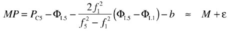
To assess the quality of the raw GPS measurements, we made use of the so-called multipath combination of pseudorange and carrier-phase measurements:
The combination is essentially the difference between the pseudorange (PC5) and carrier-phase measurement (ΦL5) on the L5 frequency, and therefore measures the sum of the pseudorange multipath (M) and noise (ε). Due to the opposite sign of ionospheric path delays on code and phase measurements, an ionospheric correction is used in the multipath combination, which requires phase measurements on a second frequency (in this case L1). The individual carrier-phase biases are, furthermore, aggregated into a common bias (b). Other than in a traditional zero-baseline test, the multipath combination neither requires a second receiver nor a second satellite transmitting the same signal in space. It is therefore best suited for studying the tracking performance of the new GPS L5 test signal.
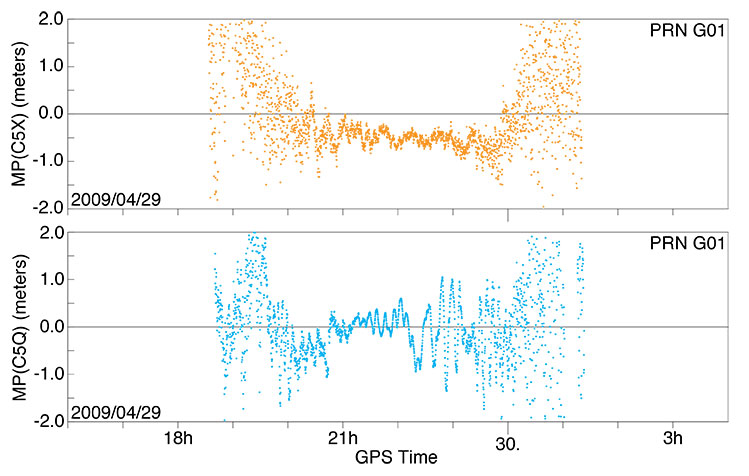
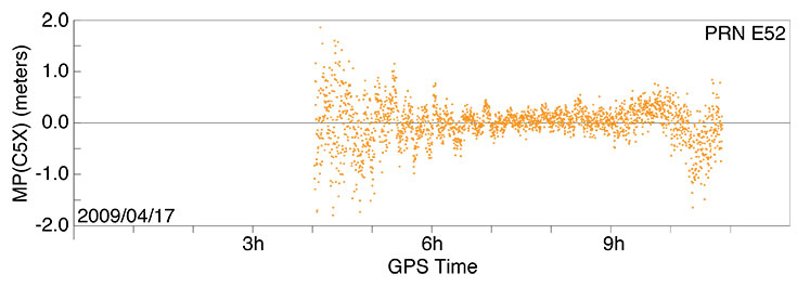
Results for receiver types N and J obtained at DLR, Oberpfaffenhofen, are shown in FIGURE 9 for a sample, high-elevation angle tracking pass. Despite obvious differences that can be related to the specific multipath environment and code-smoothing strategies for the two receivers, a high quality is obtained in both cases. For the central three-hour interval, during which the L5 signal was received with normal signal strength, the achieved tracking accuracy clearly outperforms that of the L1 C/A-code signal for the given receivers. For further comparison, FIGURE 10 shows sample results of GIOVE-B E5a tracking with receiver type J. Again, the GPS L5 signal at medium- to high-elevation angles is fully competitive and a notable degradation is only evident when the signal strength is well below the values to be expected in the future operational system.
FIGURE 9. Pseudorange multipath and receiver noise of SVN49 (PRN G01) L5 tracking for a selected pass over Oberpfaffenhofen, Germany, on April 29-30, 2009. Top: receiver type J with geodetic antenna. Bottom: receiver type N with a Galileo antenna. The satellite exceeded an elevation angle of 50° between 20:30 and 23:30 with a peak elevation angle of 80° near 22:00.FIGURE 10. Pseudorange multipath and receiver noise of GIOVE-B L5 tracking for a high pass over Oberpfaffenhofen, Germany, on April 17, 2009, using receiver type J.
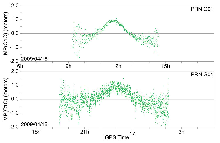
Legacy Signal Anomaly. While the GPS L5 signal transmission by SVN49 is clearly designated as experimental, the legacy signals (that is, the C/A- and P(Y)-code on L1 as well as L2C- and P(Y)-code on L2) were expected to achieve the same level of performance as observed on other satellites of the existing constellation. This is not the case, however, in the L1 band where both the C/A-code measurements and the semicodeless P(Y)-code pseudoranges exhibit a systematic, elevation-angle-dependent bias. This bias is not specific to any of our test receivers and can be similarly observed in heritage receivers employed at the stations of the International GNSS Service (IGS). As an example, FIGURE 11 illustrates the variation of the C/A-code error for high-elevation angle passes of SVN49 over western Canada and Germany. The bias varies between approximately -0.5 meters near the horizon and 1meter near zenith.
The cause of the bias is unclear but resides apparently in the design of the transmitter antenna or signal generation chain. It is exclusively seen on SVN49 and not on other GPS (or GIOVE) satellites, which excludes a possible problem of the receiver antenna or environment. Furthermore, data collected at UNB using the UNBJ IGS station a few days after launch clearly demonstrate that the elevation-angle-dependent L1 bias existed well before L5 signal activation and therefore might not be related to the signal generator. It is unclear to what extent the L1 signal bias can be corrected on the spacecraft and how it will affect the declaration of SVN49 as a fully healthy satellite.
FIGURE 11. Pseudorange errors of SVN49 L1 C/A code tracking for high-elevation-angle passes using a type A receiver at IGS station DRAO in Penticton, Canada (top), and a type J receiver at Oberpfaffenhofen (bottom). The satellite achieved peak elevation angles of about 70° and 80°, respectively, at the two sites.
Conclusions
Tracking and analysis of SVN49’s L5 signal using both the 30-meter dish and code-correlating receivers reveals that it possesses improved signal characteristics with respect to the legacy signals, in particular with regard to its bandwidth, and therefore will allow even more accurate and reliable positioning when the signal is deployed on the future Block IIF constellation.
Acknowledgments
We thank NovAtel and JAVAD GNSS for supplying special firmware, Sébastien Carcanague at UNB, and DLR colleagues at Weilheim for their help. The L5 signal description comes from the Innovation article by A.J. Van Dierendonck and C. Hegarty, September 2000 issue of GPS World.
Manufacturers
Receiver N is the NovAtel (www.novatel.com) EuroPak-15a. Receiver J is the JAVAD GNSS (www.javad.com) Triumph Delta-G2T. Receiver A is an Allen Osborne Associates (AOA) Benchmark ACT (www.itt.com). Space Engineering (www.space.it) Galileo Experimental Sensor Station antenna, Trimble (www.trimble.com) Zephyr Geodetic II antenna, and AOA D/MT antennas were used.
MICHAEL MEURER received a Ph.D. in electrical engineering from the University of Kaiserslautern, Germany. He is director of the Department for Navigation in the Institute for Communications and Navigation of the German Aerospace Center (DLR).
STEFAN ERKER received his diploma degree in information technology from the Technical University of Kaiserslautern and works at DLR’s Institute for Communications and Navigation.
STEFFEN THÖLERT received his diploma degree in electrical engineering from the University of Magdeburg and works at DLR.
OLIVER MONTENBRUCK works at DLR’s German Space Operations Center, Oberpfaffenhofen, where he is head of the GPS Technology and Navigation Group. He holds a Dr.rer.nat degree in physics.
ANDRÉ HAUSCHILD received his diploma degree in mechanical engineering from the Technical University of Braunschweig, Germany, and is a Ph.D. candidate at DLR’s German Space Operations Center.
Further Reading
L5 Signal Details
Interface Specification, IS-GPS-705 (IRN-705-003), Navstar GPS Space Segment/User Segment L5 Interfaces, ARINC Engineering Services, LLC, El Segundo, California, September 22, 2005.
“The New L5 Civil GPS Signal” by A.J. Van Dierendonck and C. Hegarty in GPS World, Vol. 11, No.9, September 2000, pp. 64–72.
DLR’s GNSS Verification and Analysis Facility
“GNSS Signal Verification: Spectral and Temporal Analysis of GIOVE B and BEIDOU Signals” by S. Thölert, S. Erker, M. Cuntz, M. Meurer, U. Grunert, and J. Furthner, presented at Navitec 2008, the 4th ESA Workshop on Satellite Navigation User Equipment Technologies, Noordwijk, The Netherlands, December 10–12, 2008.
“GNSS Signal Verification with a High Gain Antenna – Calibration Strategies and High Quality Signal Assessment” by S. Thölert, S. Erker, and M. Meurer in Proceedings of ITM 2009, the 2009 International Technical Meeting of The Institute of Navigation, Anaheim, California, January 26–28, 2009, pp. 289-300.
Nonlinearities in Microwave Signal Components
“Frequency-independent and Frequency Dependent Nonlinear Models of TWT Amplifiers” by A. Saleh in IEEE Transactions on Communications, Vol. 29, November 1981, pp. 1715–1720.
“Analysis of GIOVE-A L1-Signals” by S. Graf and C. Günther in Proceedings of ION GNSS 2006, the 19th International Technical Meeting of the Satellite Division of The Institute of Navigation, Fort Worth, Texas, September 26-29, 2006, pp. 1560–1566.
Commercial GNSS Receivers Used for L5 Signal Acquisition
“Triumph Technology” by J. Ashjaee presented at the 5th Allsat Open Conference, Hannover, Germany, June 19, 2008.
“A Dual-frequency L1/E5a Galileo Test Receiver” by N. Gerein, M. Olynik, M. Clayton, J. Auld, and T. Murfin in Proceedings of the European Navigation Conference – GNSS 2005, Munich, Germany, July 19-22, 2005.
The Multipath Observable
“TEQC: The Multi-Purpose Toolkit for GPS/GLONASS Data” by L.H. Estey and C.M. Meertens in GPSSolutions, Vol. 3, No. 1, 1999, pp. 42–49.
1995 Reports on the Future of GPS
The Global Positioning System: Charting the Future: Charting the Future by a panel of the National Academy of Public Administration and by a committee of the National Research Council, National Academy of Public Administration, Washington, D.C., 1995, ISBN 0-9646874-1-0.
The Global Positioning System: A Shared National Asset, Recommendations for Technical Improvements and Enhancements by the National Research Council Committee on the Future of the Global Positioning System, National Academy Press, Washington, D.C., 1995, ISBN 0-309-05283-1.
The Seminal Article on the Benefits of Three GPS Signal Frequencies
“The Promise of a Third Frequency” by R.R. Hatch in GPS World, Vol. 7, No. 5, May 1996, pp. 55–58.
Was the FGDC Mortgage Crisis Meeting a Silver Lining on a Huge Cloud?
By Art Kalinski, GISP
On May 7, I attended a special meeting addressing the mortgage crisis hosted by the Federal Geographic Data Committee (FGDC) and the International Association of Assessing Officers (IAAO). The purpose of the day long meeting was to discuss the use of land parcel data in managing mortgage related issues. The meeting focused on how GIS can monitor and manage these issues and to get feedback from leaders on which specific data elements are important to the mortgage industry and its financial oversight. The meeting was held at the American Institute of Architects Building in Washington, D.C.
The participants included representatives from banking, finance, credit, and mortgage firms as well as members of federal regulatory agencies. Also present were GIS professionals, private sector solution providers, and land parcel data producers. The meeting was opened by Dr. David Moyer, the meeting facilitator; Mike Howell, OMB and vice chair of the FGDC Steering Committee; Bob Ader, co-chair of the FGDC Cadastral Committee; and Dr. Josephine Lim, president of the IAAO.
Key presenters in the morning sessions were Anne Hale Miglarese of Booz Allen Hamilton, the chair of the National Geospatial Advisory Committee (NGAC); Dr. Dave Cowen, a leading GIS educator; and Dr. Nancy von Meyer who has worked on cadastral issues for over 20 years, including her current work for the U.S. Bureau of Land Management (BLM).
According to the presenters, some analysts and GIS professionals saw the mortgage crisis coming but there was also a lot of “whistling past the grave yard,” as people hoped that the trend would not turn into a crisis. The rise in distressed mortgages, foreclosures, and decreasing real estate values were visible long before the crisis became a crisis. Key to monitoring the issues was good parcel level data. Unfortunately, even though we have high tech tools such as GIS, there are institutional barriers that limited the effectiveness of those tools. There was a lack of consistency and interoperability of key datasets at a national level.
I personally experienced two such frustrations related to the post office and to the census. When I first joined the Atlanta Regional Commission (ARC) as the GIS Manager in 1993, I learned that ARC published zip code maps as a service to the regions’ economic development offices. My response was “why don’t they get them from the post office?” After all, during my graduate work at the University of North Carolina we constantly used zip code marketing data for site selection and trade area analysis. I assumed that the zip code polygons came from the source, the U.S. Postal Service. I was wrong.
In the pre-GIS age, when zip codes were created, the purpose was to build delivery routes not defined polygons. As a result, the zip code boundary files we use are very fuzzy and the polygons only approximate boundaries. I was so incredulous, that I personally drove up one major road in Cobb County to conduct my own survey. What I saw were businesses in one long block on the same side of the street that had alternating zip codes as one progressed up the street. I was told that this happened because the business where given a choice of having a Marietta city address or a Kennesaw city address. This, of course, is one example of one street in one county, but my understanding is that this is a system wide issue. Even today the Postal Service doesn’t publish zip code maps but instead refers users to commercial vendors who create zip code maps. Of course these commercial maps come with disclaimers regarding the validity and positional accuracy of the data.
The second frustration was helping with the U.S. Census 2000 Local Update of Street Addresses (LUCA). Under this census program, local talent was used to update TIGER street data and addresses. The key limitation was that we all had to sign confidentiality agreements that any data collected and any data sets that were enhanced with this collection effort would also be confidential. That meant that if I sent staff to a new neighborhood and identified new streets and news addresses, not even houses, just address locations, that information was confidential and if I used the information to update our massive ARC street centerline database that file also became confidential.
I could then send the same people out on a different day to the same location to collect the same data but if the data collection was not in the name of LUCA, it was not confidential and we could use it. Yes, I fully appreciate privacy but the mere existence of a street address tells you nothing about the parcel or the building, if there is one, or even the inhabitants, if there are any. In fact, most of this data in even greater detail is already available from commercial sources. These are just two examples that hurt data collection and interoperability, but there are more when it comes to parcel level data. Now I’m about as conservative as one gets, but this silliness in the name of privacy defies common sense and is an example of how we twist ourselves into knots to our own detriment.
The afternoon sessions were facilitated by David Stage of the FGDC Cadastral Subcommittee, Susan Marlow of Smart Data Strategies, and Roger Clark of IAAO. The meeting focused on obtaining feedback from users in the mortgage industry as to specific data they need to do their job effectively. The list of data elements included factors that one would expect. There was a large list related to the property descriptions, such as lot and building size, construction — several attendees highlighted the need for street level or oblique imagery of each property, and annotation of the condition of improvements. George Donattelo of IAAO indicated that these were especially needed if IAAO AVM and Mass Appraisal Standards are used. Financial factors included the type of mortgage, equity, and terms of the mortgage. Geospatial factors such as nearness to water, flood plains, neighborhood comparable appraisals, demographics, and regional economic factors such as employment levels added even more complexity to the analysis.
The discussions all pointed to the need for timely analysis using comprehensive data. We know that spatial analysis of all factors, perhaps with regression analysis, could help with future forecasting, but analysts need data that is detailed, accurate, and most importantly, consistent. There was a general consensus that just a small portion of the rescue funds should be devoted to creation of comprehensive data collection efforts. All agreed that this should be the message from this meeting to our leaders.
I’m hoping that this economic crisis will open everyone’s eyes to the need for consistent and comprehensive data if government is going to insert itself into the market. Homer Simpson one stated: “Beer, the cause of and solution to life’s problems.” … Dare I substitute “government” for “beer?” Maybe with superb data and competent analysis we can look back on this crisis with open eyes and not repeat our mistakes. Perhaps the realization that we need good data and GIS analysis will be the silver lining.
A few short weeks ago, the U.S. GPS program had its posterior firmly planted in the catbird seat. Government spokespeople in international fora looked on benignly as European, Chinese, and Russian GNSS programs struggled to resolve their issues and meet their heady challenges. All was well with the world. A new GPS satellite launched, a segment of radio-frequency spectrum secured for a promising new signal, a next-gen satellite shipped to the Cape, and the next-next-gen program nearing successful preliminary design review (since completed).
In the blink of an eye, the world is turning.
A progression of seemingly unrelated events began to affect GPS outlook.
While successfully broadcasting the new L5 signal, IIR-M (20) also began generating “out of family” measurements on L1 and L2 at low elevations.
The long-withheld Independent Assessment Team (IAT) report on eLoran appeared, unanimously recommending that “the U.S. government complete the eLoran upgrade and commit to eLoran as the national backup to GPS for 20 years.” While in itself this is good news — that is, if you believe in backing up critical systems — it does not augur well that a two-year Freedom of Information Act fight had to be waged to pry the report loose from know-nothings in the Department of Homeland Security, and that the vaunted Obama administration, heralded as a breath of change, had earlier come down on the same-old same-old government side of taking Loran out.
Then, the motherlode. The U.S. Government Accountability Office (GAO) issued a report on the future of GPS, characterizing the constellation as susceptible to falling below full operational capability between 2010 and 2018.
It turns out that while a IIF payload did travel to Cape Canaveral on May 7, this was solely for the purpose of preliminary launch-system compatibility testing. The satellite itself is not ready to operate in space, and in fact the IIF currently at the Cape is just a placeholder. Or, to use press-release verbiage, to “serve as a risk-reduction pathfinder for SV1 processing later this year.” The real satellite, the IIF that may, repeat may, go into orbit at the end of this year or early next year, continues in critical payload testing at the contractor facility.
Here’s a bright spot, at long last. Brad Parkinson, the first GPS Program Office Director, chief architect and advocate for GPS, has a plan for mitigating possible GPS brownouts — the gaps in service that may occur if the constellation should fall below quorum. Parkinson states that “It is possible that the constellation will be at a level of less than 24 satellites. I would like to focus on the options that would help reduce this risk.”
Parkinson cites two principal causes for the current at-risk status of GPS service. “The first is that the generation of replacement satellites called IIF has been greatly delayed. A substantial part of the reason for this is that the contract for IIF satellites was placed during a period when DOD imposed a grand experiment in contracting. In addition there were some changes to the satellite to modernize its design, but the bottom line is the satellite has been on contract since 1996 and will not be launched until 2010. The design is quite old, and the capability of the satellites does not meet the latest requirements.”
The second cause is protracted delays by the decision-making and budgeting processes in getting Block IIIA going. These issues have now been resolved, and Parkinson points out that both reasons “are now a matter of history. The current issue, that should concern us all, is: what options should we pursue to substantially reduce the risks of brownout.”
Parkinson makes three recommendations in his personal presentation to the PNT Advisory Board meeting; the same presentation was also submitted as written testimony to the Congressional hearing following on the GAO report. Download the full Powerpoint file, with written details.
“In my view, there are three major options for mitigating brownouts. Fortunately, these options could be done together. These are:
To reactivate the previously retired GPS satellites that are still operating in normal GPS orbits.
To speed up the GPS IIIA development space (expedite the milestone approvals).
To develop a simplified GPS IIIA based design, Spartan satellite (IIIS) that would not include the extra payloads, and, once designed, could be built quickly and launched into space with two satellites on a booster. This would be done in parallel with the current program.”
Dr. Parkinson adds that “There is a fourth option, which may have been offered by some. This is to restart or expand the GPS IIF production line. The apparent advantage of this is that the GPS IIF is close to its first launch. Some might think major advantage would have been the fact that it is already designed. Weighing against this advantage is the fact that the design and the parts are obsolete. Virtually all the boxes and components would have to undergo a major redesign. Furthermore, the design is still untried, and was developed during an era of flawed procurements.”
Counterpoint. Boeing says its engineers are working “very closely with the Air force and its team” and that the company has taken “aggressive steps to resolve the technical issues on IIF with a strong emphasis on mission assurance.” It maintains that it is on track to deliver the first IIF satellite, ready for launch, later this year.
“Boeing’s GPS IIF satellites,” the press release continues, “will deliver more capability and improved mission performance to military and civilian users. . . . Design changes were required to ensure performance over the satellite design life and these have caused schedule delays, but these changes are in the final phase of implementation and a fully integrated satellite (SV1) has already successfully completed the thermal-vacuum test program — the most stressing system level test. SV2 was shipped to the Cape (Canaveral) on May 6 to perform system-level compatibility tests and serve as a risk reduction pathfinder for SV1 processing later this year.”
The Department of Defense also made a presentation to the May 14–15 National Space-Based PNT Advisory Board meeting, and in it highlighted three risks: delay of IIF, delay of the ground control segment (OCX) contract award, and delay of GPS IIIA.
Some in the GNSS community feel that the GAO-generated furor focuses too much on Block IIF and not enough on these other unknowns. They foresee a strong likelihood that the IIF satellites will get aloft on time, suitably “following on,” as they have been named. The real scary part will come later, in the 2015-2017 timeframe when GPS IIIA doesn’t get into orbit in sufficiently quick
numbers.
Further, the GAO report did not account for two mitigation tools that the DoD has in reserve: three retired satellites still in space that could be brought back into operation, and power-shedding as a means to extend satellite life.
Back to the Mitigation Talk.Coming up are some of the strongest words Parkinson employed in the PNT Advisory Board presentation: further congenital defects.
“While the Air Force has undertaken a very rigorous test program,” read the presentation notes, “it is still conceivable that we will find further congenital defects. The IIF satellite lacks the powerful military signal that will be extremely helpful against potential hostile jammers. In addition, it does not broadcast the new international signal L1C. Because of the extensive redesign it seems probable that the satellite would have to be re-competed. Finally, this would be a major near-term budget hit in a period when the IIF satellite is still over running its budget.”
Not Even Half the Picture. GPS program planners have one of the most complex tasks going. They must consider many other issues in addition to keeping an integer number of satellites flying. Dual handling of the space and ground segments while both undergo modernization so that they remain in phase with each other, further synchronization with military user equipment on its own track of development, operating under a leadership and decision-making structure that lacks unity at the top, structuring future interoperability with other GNSS neither aloft nor complete in their signal-structure design — and then the various PR issues involved with servicing a worldwide, multinational, multi-industry, multi-requirement customer base.
Personally, I feel much more comfortable here in my armchair.
And despite all the grim news this month, I remain confident that GPS will continue to lead the field of GNSS, providing exemplary service round the clock, round the world.
Brad Parkinson, the first GPS Program Office Director, chief architect and advocate for GPS, submitted written testimony to Congress on mitigation options for possible GPS brownouts. His presentation comes in reference to the recent GAO report highlighting the risk that the GPS constellation may fall below the minimum level of 24 satellites required for full operational capability. In his opening, Parkinson states that “GAO correctly points out the possibility that the GPS constellation will be reduced to less than the current number of 30 to 32 satellites. In fact, it is possible that the constellation will be at a level of less than 24 satellites. I would like to focus on the options that would help reduce this risk.”
Parkinson chides those who may not have been paying attention over the last two years, at least. “It should be noted that the risk of brownouts has been repeatedly pointed out by the independent review teams,” he states, referencing the the Defense Science Board, the GPS Independent Review Team, and the Pos-Nav Timing Advisory Board, who have all stated all that “30 satellites is the correct number.” He points out that the European Galileo program and the Chinese Compass system have also arrived at that number.
“Although brownouts would only be ‘officially’ declared at levels below 24, anything below the current level of 30 satellites is a cause for concern. The potential economic impact if the number were below 24 may be quite serious.”
To rectify the situation, Parkinson first gives a history lesson. The first GPS satellite went from contract award to launch in 44 months. “The keys to success were a streamlined approval chain (all the way up the OSD chain), severe restrictions on any contract changes, and an integrated product team.” He believes that GPS IIIA can achieve the same — given the same playing conditions.
Spartan. He does throw in one twist not currently in the plans: “To develop a simplified GPS IIIA based design, Spartan satellite (IIIS) that would not include the extra payloads, and, once designed, could be built quickly and launched into space with two satellites on a booster. This would be done in parallel with the current program.”
Parkinson appears to advocate complete abandonment of the IIF line. “The reason is simply that the satellite design is old and relies on parts that are no longer available. In addition, the satellite, while providing the older signals, does not meet current requirements.”
He closes with a final admonition. “Above all, the senior decision making chain has to become a part of the solution. This means that they do everything in their power to help the program office achieve the needed schedule.”
Withheld from the public for two years, since its completion in March 2007, the Independent Assessment Team (IAT) report has been let out of detention, just in time to counter recent efforts by the Obama administration, the Department of Homeland Security, and the U.S. Coast Guard to throttle the program. The IAT “unanimously recommends that the U.S. government complete the eLoran upgrade and commit to eLoran as the national backup to GPS for 20 years.” The IAT’s conclusion has long been informally known throughout the GPS industry, but the report’s release adds considerable weight, expertise, and specifics to a long, determined campaign to preserve the program.
Compiled by the Institute for Defense Analyses, the IAT report has been held back from public release since March 20, 2007, when it was completed and presented to the co-sponsoring Department of Transportation and Department of Homeland Security (DHS) Executive Committees. Its release now comes only after an extensive Freedom Of Information Act (FOIA) battle waged by industry representatives against the federal government.
The report asserts that “eLoran is the only cost-effective backup for national needs; it is completely interoperable with and independent of GPS, with different propagation and failure mechanisms. . . . It is a seamless backup, and its use will deter threats to U.S. national and economic security by disrupting (jamming) GPS reception.”
The IAT, chaired by Bradford Parkinson, founding program director for GPS, and assisted by other industry experts, evaluated all available or potential alternatives for a GPS backup. In particular, it examined the costs of the Loran system and a transition to a new, modernized enhanced or “eLoran.” It found eLoran’s infrastructure enhancements to be 70 percent complete, and the cost to complete its rollout less expensive than decommissioning the Loran system.
The two-year-old report finally arrives in public view, staking out direct opposition to recent comments made by the DHS that Loran termination will save $190 million over five years. Such claims failed to specify or include the decommissioning costs, or explore the operational savings available with modern eLoran transmitters. Senior DHS representatives have — unbelievably, but yes, it is true — claimed recently that it is not clear a GPS backup is needed, and have taken the time-honored route of recommending additional study.
The IAT report concludes that “eLoran be completed and retained as the national backup system for critical safety of life, national and economic security, and quality of life applications currently reliant on position, time, and/or frequency from GPS.” Its authors emphasize that “the U.S. government policy decision is needed to motivate users to equip.”
The United States Government Accountability Office (GAO) issued on May 7 an alarming report on the future of GPS, characterizing ongoing modernization efforts as shaky. The agency appears to single out the IIF program as the weak link between current stability and ensured future capability, calling into doubt “whether the Air Force will be able to acquire new satellites in time to maintain current GPS service without interruption.” It asserts the very real possibility that “in 2010, as old satellites begin to fail, the overall GPS constellation will fall below the number of satellites required to provide the level of GPS service that the U.S. government commits to.”
Prepared at the request of the U.S. House of Representatives’ Subcommittee on National Security and Foreign Affairs, Committee on Oversight and Government Reform, and titled “Global Positioning System: Significant Challenges in Sustaining and Upgrading Widely Used Capabilities,” the report concludes that “it is uncertain whether the Air Force will be able to acquire new satellites in time to maintain current GPS service without interruption. If not, some military operations and some civilian users could be adversely affected.”
“In addition,” the report summary continues, “military users will experience a delay in utilizing new GPS capabilities, including improved resistance to jamming of GPS signals, because of poor synchronization of the acquisition and development of the satellites with the ground control and user equipment. Finally, there are challenges in ensuring civilian requirements for GPS can be met and that GPS is compatible with other new, potentially competing global space-based positioning, navigation, and timing systems.”
Among the report’s principal recommendations is a proposal often made in past years by a range of experts, but never implemented: the Secretary of Defense should appoint “a single authority to oversee the development of GPS, including space, ground control, and user equipment assets, to ensure these assets are synchronized and well executed, and potential disruptions are minimized.”
While the Department of Defense (DoD) concurred with this recommendation, and while quite possibly it might effectuate the streamlined decision-making and corollary processes to remedy the highlighted deficiencies, it would run counter to the integral “dual-use” principle of GPS as dedicated to both civil and military users. Such a move could thus conceivably and adversely affect the interests of civil users.
Testimony from invited GPS providers and users before a related National Security Subcommittee hearing (“GPS: Can We Avoid a Gap in Service?”), some of which is briefly encapsulated within this news story, can be downloaded.
Why GAO Did This Study. A highlights document attached to the GAO report asserts that GPS “has become essential to U.S. national security.” The GAO conducted its own analysis of Air Force satellite data, in addition to interviewing key officials and analyzing program documentation. Specifically, the agency assessed progress in:
acquiring GPS satellites
acquiring the ground control and user equipment necessary to leverage GPS satellite capabilities
coordinating efforts among federal agencies and other organizations to ensure GPS missions can be accomplished.
Gloomy Outcomes. Based on the most recent satellite reliability and launch schedule data from March of this year, the estimated long-term probability of maintaining a constellation of at least 24 operational satellites falls below 95 percent during fiscal year 2010 and remains below 95 percent until the end of fiscal year 2014, at times falling to about 80 percent. Program officials provided no evidence to suggest that the current mean life expectancy for satellites is overly conservative, the GAO stated.
The results of fewer than 24 operational satellites could include:
Intercontinental commercial air carriers may have to delay, cancel, or reroute flights.
Enhanced-911 response to emergency calls could lose accuracy, particularly operating in urban and mountainous environments — exactly where emergencies tend to be most dire and hardest to locate.
Accuracy of precision-guided munitions could decrease, forcing the military to use larger munitions or use more munitions on the same target to achieve the same level of mission success, and increasing the risks of collateral damage. The urgent desire to decrease or eliminate collateral damage to civilians in or near conflict zones has often been cited by the founders of GPS as one of their key motivations in envisioning the program.
Both standard positioning service and precise positioning service could suffer, impacting large numbers of civil users, both professional (for example, surveyors) and casual (users of location-based services via cell phones) in moderately mountainous areas, in large cities, and under forest foliage.
Block IIF at the Crux. Cristina T. Chaplain of the GAO presented the report to Congress, stating, “In recent years, the Air Force has struggled to successfully build GPS satellites within cost and schedule goals; it encountered significant technical problems that still threaten its delivery schedule; and it struggled with a different contractor. As a result, the current IIF satellite program has overrun its original cost estimate by about $870 million and the launch of its first satellite has been delayed to November 2009 — almost three years late.”
The GAO reports cites specific problems with the IIF satellites contracted to Boeing. During the first phase of thermal vacuum testing in 2008, one of the test payload’s transmitters failed; consequently, the program suspended testing in August 2008 to identify the causes and take corrective action. Other hang-ups include maintaining the proper propellant fuel-line temperature, delaying final integration testing, and re-design of the satellite’s reaction wheels, used for pointing accuracy, because of on-orbit failures on similar reaction wheels on other satellite programs. Overall, about $10 million additional have accrued to program, according to the GAO.
“Further, while the Air Force is structuring the new GPS IIIA program to prevent mistakes made on the IIF program, the Air Force is aiming to deploy the next generation of GPS satellites three years faster than the IIF satellites. GAO’s analysis found that this schedule is optimistic, given the program’s late start, past trends in space acquisitions, and challenges facing the new contractor.
“Of particular concern is leadership for GPS acquisition, as GAO and other studies have found the lack of a single point of authority for space programs and frequent turnover in program managers have hampered requirements setting, funding stability, and resource allocation.
“If the Air Force does not meet its schedule goals for development of GPS IIIA satellites, there will be an increased likelihood that in 2010, as old satellites begin to fail, the overall GPS constellation will fall below the number of satellites required to provide the level of GPS service that the U.S. government commits to. Such a gap in capability could have wide-ranging impacts on all GPS users, though there are measures the Air Force and others can take to plan for and minimize these impacts.
“In addition to risks facing the acquisition of new GPS satellites, the Air Force has not been fully successful in synchronizing the acquisition and development of the next generation of GPS satellites with the ground control and user equipment, thereby delaying the ability of military users to fully utilize new GPS satellite capabilities.
“Diffuse leadership has been a contributing factor, given that there is no single authority responsible for synchronizing all procurements and fielding related to GPS, and funding has been diverted from ground programs to pay for problems in the space segment. DoD and others involved in ensuring GPS can serve communities beyond the military have taken prudent steps to manage requirements and coordinate among the many organizations involved with GPS. However, GAO identified challenges in the areas of ensuring civilian requirements can be met and ensuring GPS compatibility with other new, potentially competing global space-based positioning, navigation, and timing systems.”
Staving Off Disaster. In the course of its interviews with key officials, the GAO learned of and reports on some alternatives that have been examined. The Air Force Scientific Advisory Board considered the use of smaller GPS satellites in 2007. These could be developed more quickly and at lower cost. The board concluded that while small satellites could at some point serve to augment GPS capabilities, they would require a different and much more extensive ground control segment, program development would take too long, and necessary changes to user equipment would render the whole scheme cumbersome.
The effects of satellite power loss over time, due to harsh space conditions, could be mitigated by shutting down satellite subsystems when not needed, reducing power consumption, also by shutting off a secondary (unnamed) GPS payload. DoD has long been reluctant to take either measure absolutely, particularly the second one, but according to testimony (see below) has been implementing both practices on an intermittent basis.
Day in Congress. Other GPS community representatives testified to the House Oversight and Government Reform’s subcommittee on National Security and Foreign Affairs, alongside GAO spokesperson Chaplain.
According to Lt. Gen. Larry D. James, Commander, 14th Air Force, Air Force Space Command, and Commander, Joint Functional Component Command for Space, U.S. Strategic Command, the Space Command maintains the required minimum of at least 24 GPS satellites in orbit, and the current level of 30 operational satellites, by keeping a “ghost fleet” of older, partially mission-capable satellites in backup mode. “Currently, three vehicles are held in residual status and are returned to the constellation every six months to ensure operational capability.” He stated that added life also is being squeezed from the satellites by reducing power to or turning off equipment for secondary missions aboard the satellites.
Karen Van Dyke, acting director for Positioning, Navigation and Timing in the U.S. Department of Transportation’s Research and Innovative Technology Administration (RITA), told the Congressional committee that “GPS is vulnerable to interference that can be reduced, but not eliminated.” Citing the 2001 Volpe Report for which she was a key author, she stated that there has long been “an awareness within the transportation community of risks associated with use of GPS as a primary means for position determination and precision timing. Due to the reliance of transportation on GPS signals, it is essential that threats be mitigated and alternative back-ups be available, and the system be hardened for critical applications. DOT has determined that sufficient alternative navigation aids currently exist in the event of a loss of GPS-based services.”
Nearly simultaneously with the GAO report and congressional hearings, the long-withheld Independent Assessment Team report on eLoran as a GPS backup has just been released.
F. Michael Swiek, Executive Director, U.S. GPS Industry Council and a member of GPS World’s Editorial Advisory Board, reminded Congress of the dual-use nature of the system, saying “The U.S. Government has promoted and encouraged [GPS] development by establishing, maintaining and reinforcing a stable policy framework that has consistently received farsighted and bipartisan support. It has been a true partnership of shared visions, discussions and debates, cooperation, and coordination. This has been possible through the open dialogue that has taken place since the early days of GPS, some 25-plus years ago, between civilian and military, industry, and government on technical and policy issues as the technology, system, and applications have evolved.”
Swiek made his recommendation that “successful adoption of modernized civilian GPS signals will occur if the installed user base can continue to trust the consistent and stable policy framework that the U.S. government has provided for GPS for two decades. The new signals will need to sustain the legacy of accuracy, availability, and reliability established over the past 20 years.”
Chet Huber, president of OnStar, a wholly owned subsidiary of General Motors Corporation, and at nearly 6 million active subscribers probably the largest single group of civil GPS users, offered three recommendations:
“First, we must address the health of the current constellation. We are concerned that a recent report shows eight of the current satellites are one component from total failure. Loss of signal will likely immediately affect GPS accuracy and availability (geographic coverage).
“Second, as the GPS system is modernized, it is imperative that the U.S. government formally commit to preserving the L1C/A signal and to ensuring backward compatibility for legacy applications with no loss of performance from current levels. . . . Any modernization initiative that degrades backward compatible performance — such as reducing the number of satellites making up the constellation — would likely adversely impact the provision of services by OnStar, including the quality of location information we provide to public safety, thereby potentially increasing the response time of public safety personnel to crash victims and others in need of emergency services.
“Our third recommendation — and this is also important to legacy applications — is that we commit to maintaining the current PRN code (or satellite signature structure) for the primary orbital slots, as satellites in those slots are replaced. Legacy hardware is not capable of being expanded to accommodate more than 32 slots so renumbering above 32 will likely affect performance of legacy applications.”
I really enjoy doing webinars and the RTK Network webinar on April 21 was no exception. One of the reasons I really enjoy them are the questions and comments I receive because it gives me some feedback as to what the user community is thinking and wondering about. Clearly, RTK networks are a hot topic these days. The registration for the RTK Networks webinar was one of the highest in history for GPS World.
Now without further ado, following are questions that listeners sent in and my comments from the RTK Networks webinar.
Question #1: Can you say anything about the proposed National Geodetic Survey Real-Time Networking (NGS RTN) guidelines?
Gakstatter: The NGS is still in the early stages of developing the RTN guidelines so the agency would prefer public comment be withheld at the moment. It’s are working on guidelines to cover four areas: site considerations; planning and design; administration; and users. The agency has assembled quite a team of government and industry people to develop these guidelines. The team hopes to have draft versions ready by September 30, 2009.
However, the NGS Real-Time User Guidelines (Ver. 2.0.4) is available to the public. Though these guidelines are targeted at classical RTK users (non-RTK network), it contains some solid procedures.
Also, an interesting study was published recently by Newcastle University Civil Engineering and Geosciences specific to network RTK. Stakeholders in the report include The Survey Association (UK), Ordnance Survey (UK), Leica Geosystems, Trimble, and Royal Institute of Chartered Surveyors. They did some extensive testing and generated basic guidelines:
Configure the rover according to manufacturer guidelines. According to the report, significant deviations from recommended settings can introduce unacceptable errors.
Consider lowering the GDOP (PDOP) mask to 3 instead of 5. Generally, in a clear-sky environment, you’re going to get this anyway and it will increase the robustness of solutions in challenging areas.
Pay close attention to quality indicators on the rover (for example, RMS values). They generally reflect actual performance of the rover. An RMS value more than 10 centimeters generally indicates there is a problem such as loss of ambiguity resolution or other satellite loss of lock. Those positions should not be used. However, in challenging environments (such as obstructed satellite visibility and multipath) quality indicators (especially vertical) maybe be “overly optimistic” by a factor of 3 to 5.
The report commented on occupation times, which I’ve written about in a previous article. Using a 5-second average on topographic will reduce the effect of individual epoch variations.When vertical is important (as in establishing secondary control), two different sessions of at least 180 seconds should be recorded. The report indicated that a time separation between sessions of 20 minutes will yield an accuracy improvement of 10 to 20 percent. A time separation of 45 minutes will yield an accuracy improvement of 15 to 30 percent. A time separation of greater than 45 minutes did not provide “appreciable further improvement. This was very interesting to me as most guidelines I’ve read (including NGS guidelines) dictate a four-hour separation between sessions.
GLONASS improves satellite visibility (thus increasing productivity), but doesn’t necessarily improve accuracy. *
This conclusion doesn’t surprise me, but I think there needs to be an asterisk here since there are significantly more GLONASS satellites available now than there were a year ago. In a scenario where there are only five GPS satellites and four GLONASS satellites, my guess is that at least the robustness of the solution will be better, and generally the accuracy as well, due to the improved geometry (PDOP).
Their recommendations make a lot of sense to me. Probably the most controversial is the separation time (45 minutes versus four hours) between sessions. This is against most standard practice that I’ve read, but then again I don’t have empirical data to support it either way, whereas the report does. It is clearly an area that needs a closer look. The time savings in the field could be reduced considerably for setting secondary control if this practice was adopted.
Question #2: What manufacturers for RTK-network implementation would you recommend?
Gakstatter: Well, there aren’t many choices. The market is dominated by Trimble and Leica Geosystems, with Topcon on the fringe.
I don’t know if anyone can say with confidence which one is better from a technology standpoint. I’ve used rovers on all three networks and all seemed to behave as expected.
Both Trimble and Leica networks have been implemented in large geographic areas (state-wide, country-wide) so they’ve experienced the growing pains and presumably have worked out any major issues.
There are many issues other than which network software vendor you select. A big one is the information technology (IT) component. Without support from your IT department (or control over IT with a competent IT project manager), getting a network to run smoothly will be a really rough road. I don’t pretend to have gone through the process of setting one up, but I’ve talked to enough people to know this is a common theme among them.
Question #3: How different is the RTK processing for network versus cluster?
Gakstatter: A cluster is essentially a group of reference stations set up in a geographic area. The user selects which reference station to use (usually the closest one) and receives corrections just like a user would from a reference station he set up himself. Communications from reference station to user is generally accomplished via UHF/VHF/spread spectrum radio or wireless network (GSM, CDMA).
With a network, data is collected by all reference stations and sent to a central server where the data is processed; corrections are generated and sent to the user. Sophisticated atmospheric modeling is done and incorporated into the corrections. In theory, this eliminates distance-dependent errors within the network.
Question #5: Does anyone know of any other published RTN user guidelines?
Question #6: Could you talk a little about post-processing?
Gakstatter: Well, it’s a subject worthy of more space than can be accommodated here, but it certainly has its place in setting primary survey/geodetic control and is the preferred method.
Also, single-frequency GPS units are still the price leaders for entry-level GPS surveying. Even today, many people use GPS L1 units with post-processing for collecting topo survey data.
Question #7: We are in Philadelphia and we use the Trimble VRS Network. We download and import a .dc file into Trimble Office. I don’t feel as confident using this network as I did when we got an OPUS solution and adjusted the base station. Procedure-wise, do you have any advice on how to capture the data? We are doing a morning session and an afternoon session and averaging the results.
Gakstatter: I deferred to Bill Henning who is the RTK network specialist with the National Geodetic Survey. NGS has developed RTK user guidelines. Here is Bill’s opinion:
“RTK will give you coordinate information and not much else. You can set the data collector to keep covariance records, which will allow you to dump the data in the office program and actually perform a tweaking of the coordinate positions if you have redundancy in some form (another location on the point of interest). I would never use just one RTK location for any significant point — there are too many variables. Any point that you will reuse or that is important in itself to the job should be located redundantly (see the summary table in Section V. of the single base guidelines). Also, any point whose elevation is important to less than 3 centimeters should be leveled (or produced from a total station shot from a known point, and so on). In another vein, typical RTK accuracies (say 0.03′ horizontal, 0.05′ vertical) can be achieved through a localization to known and trusted passive monuments surrounding the project.
My recommendation for a project site without existing trusted control would be:
Perform two OPUS-RS set-ups on the site control points. These would be 15-minute sessions staggered by 4 hours. Even better (but not usually in the cards), perform the second session on a different day and/or with different weather (still staggered by 4 hours, though). Site control should form a rectangle around the project with additional internal control for large sites.
Use the RTN to check values on the OPUS-derived coordinates. This is where the datums and epochs of the RTN come into play! If the RTN is using coordinates aligned to the NSRS within a couple of centimeters, all should be well (to that accuracy). Search for outliers. Evaluate these for the error source (user, OPUS, RTN) and correct or discard.
Perform a site “localization” to the site control from the RTN. This will let the user now use the RTN for internal work based on the site control as the “truth.” This is most important for the verticals. All features that require an elevation accuracy RMS less than 0.05′ (say 1.5 cm), should be done redundantly or better, by more precise means such as leveling or total stations.
Make sure of the integrity of the site control for future work. Points should be outside of the disturbance area with good stability.
Question #8: How do you feel about the appropriateness of RTK for “boundary” locations? What QA/QC can be done in the field?
Gakstatter: Many surveyors I know use RTK for setting boundaries. Some even use single-baseline RTK for this task, which is essentially just a radial survey (no redundancy). I’d say that almost all who I know that are doing this have used their RTK systems enough to understand the limitations. In fact, I think most have run RTK and total stations side-by-side on jobs to gain confidence and understand RTK in the field.
I’m sure I’ll get blasted by some folks for not downplaying RTK for determining boundary locations, but I don’t think it serves any purpose to ignore what’s actually happening in the field. There is so much pressure, especially in these economic times, to reduce field time and increase efficiency that RTK ends up filling that need.
At a minimum, I would occupy each point at least twice with the base station set up on two different monuments. If you’re using corrections from an RTK network, I’d occupy twice with a 4-hour separation between occupations (for example, once in the morning and once in the afternoon). I’d even dump the antenna a couple of times with each occupation to get two or three “fresh” measurements.
The above assumes that you have a clear view of the sky (no blockage by trees or buildings), are tracking at least six GPS satellites, and have a PDOP of 3 or less. If you’re up against a tree line, tracking five satellites, and the PDOP is 5, I wouldn’t accept it even if the RMS indicators looked good.
I’ll leave at that for now, as I could write a column just on this subject. I certainly would not support someone new to RTK to cut their teeth on boundary locations. I’d suggest building confidence and experience with RTK on applications where there is more wiggle room.
Question #9: Could you address the ability of the RTK network or cluster to adequately service dynamic surveys verses static?
Gakstatter: Dynamic is really the issue here. In my experience, there are at least a couple of issues to be aware of.
There’s generally a “lag time” between when you press the button on the data collector and when the measurement is taken. I don’t have any empirical data on this, but it’s something I’ve experienced and I’ve seen that some make and models of equipment do better than others. If you’re moving at 8 mph on a 4-wheeler and the lag time between pressing the data collector button and the actual measurement is 1 second, you will travel approximately 12 feet before the measurement is recorded.
A few years ago, a client of mine wanted to measure the acceleration of a vehicle after it was impacted by another vehicle. We determined that recording data at 1 Hz (one measurement per second) wouldn’t provide sufficient resolution. Nearly all RTK systems come preset to record at 1 Hz. However, most RTK equipment is able to record faster than 1 Hz. We ended up recording at 10 Hz (10 measurements per second).
Question #10: It is possible to use a single-frequency receiver as a rover in the RTK technique, or it is a limitation?
Gakstatter: I’ve got just a little experience in attempting to use L1 RTK on an RTK network. It didn’t work very well for me for centimeter-level accuracy, but worked OK for sub-foot accuracy.
L1 RTK systems generally have some specific needs in order for them to work optimally. For example, some are able to utilize SBAS satellites as observables. RTK networks don’t support this type of observable (at least the ones I know of), so optimal performance from L1 RTK is achieved when the user operates his or her own reference station instead of using an RTK network.
Question #11: You should discuss the advantages of using PPP if a reference survey monument is not available when setting up/initializing RTK.
Question #12: For the states out west, any challenges you are aware of in collaborating with the PBO on upgrading stations to real time and receiving the raw data?
Gakstatter:Plate Boundary Observatory (PBO) has a tremendous number of reference stations in the Western United States, I think more than 800. I’ve spoken to a few different RTK network administrators in the Western U.S. who have incorporated PBO reference stations into their RTK networks. The general consensus is that PBO site communications is the major challenge. RTK networks require that the data stream travels from each reference station to the network server and then to the user within two seconds, so reliable communications is very important. PBO sites weren’t designed for this sort of communications in mind so that portion has to be upgraded in order for it to serve in an RTK network.
For new PBO sites, I’ve talked to an RTK network operator who has collaborated with PBO successfully in building the site and including “RTK-network compatible” communications facilities during site construction.
Question #13: Do you foresee penetration of GNSS RTK network technology in mass-market applications such as location-based services (LBS)?
Gakstatter: Not in the near future. LBS are not yet as much about accuracy as they are about applications — mostly navigation, family tracking, and social networking applications but many more are to come. None of these applications require the high degree of accuracy that RTK networks are built for.
Question #14: What is the estimated number of users in America? Say this year and three years later.
Gakstatter: I don’t have specific numbers, but I would say that this is one of the fastest growing areas in GNSS. It crosses many different industries such as survey engineering, construction, mining, and agriculture. Also, machine control is expected to grow worldwide at a CAGR of 23%-28% in the next five years and real-time positioning is a critical component for this.
Question #15: Does latency in cell signals affect accuracy in clusters or networks?
Gakstatter: Yes, very much so. The industry standard latency ceiling seems to be two seconds from the time the data leaves the reference station, travels back to the server, is processed, then is received by the user. Any hiccup in the communications process will affect accuracy.
Question #16: Our network recently performed a readjustment. This shifted the H by .08′ and the V by .10′. If you are using the network for real property boundaries, do you want to stay on a current epoch? Or have your property move with the crust, thus forcing recalibration on every readjustment?
Gakstatter: Again, I deferred to Bill Henning who is the RTK network specialist with the National Geodetic Survey. NGS is developing user and administrator guidelines for RTK networks. Here is Bill’s opinion:
“What has happened is either the RTN needed to be readjusted to be more accurate — due to new data, perhaps — or the RTN adopted a new realization [say NAD 83(NSRS2007) from NAD 83 (HARN)], or due to significant movement of the stations it was felt the coordinates should be maintained as current rather than at a prior epoch. For whatever reasons, you can see that the metadata on the RTN stations would be critical to consistent positioning. Because as the NGS CORS network is referenced to a particular epoch of time (ITRF 2000 realization of the ITRS at epoch 1997.0 transformed to NAD 83 realized at CORS adjustment 1996 at epoch 2002.0), with velocities supplied in both datums, the user can position from these stations to his epoch of survey by applying the shifts in coordinates produced by applying the velocities. All RTN should do the same.
“We have been spoiled in most of the U.S.A. by having a datum that moves with us and therefore has little residual movement relative to our position. NGS is now moving towards adopting a true geocentric datum aligned either to a certain epoch of a certain ITRF realization and fixed on a stable North American tectonic plate, or one that will adopt the worldwide velocities referenced in the ITRS datum. To be consistent, surveyors (and all geospatial professionals) should be sure to provide the proper metadata on their work, which will state the coordinate datum basis, source of coordinates, epoch date of the coordinates, estimated velocities as published, and whether the distances reference grid or ground coordinates. They can opt to provide coordinates based on the epoch date of the RTN or they can provide them for the date of survey, but they must provide the metadata for those following afterwards — including planners, designers, engineers, GIS, and future boundary retracers.
Question #16: Will network RTK win (render obsolete) or improve SBAS?
Gakstatter: I don’t think so. SBAS (WAAS, EGNOS, MSAS) was designed and built to serve the aviation community. That is a separate and distinct system that will be stand-alone. Aviation navigation system infrastructure won’t (and shouldn’t) share resources like we do in the commercial sector. Aviation navigation infrastructure needs to be a stand-alone system under full control of the governing aviation authority (for example, in the United States, it’s the Federal Aviation Administration).
Question #17: Are RTK clusters/networks providing services for users that were once only available through the National Differential GPS stations?
Gakstatter: Not really. NDGPS is one source of DGPS corrections. WAAS is another source, and there are also commercial DGPS correction providers such as OmniSTAR. RTK networks are one more that can be added to the list.
Although RTK networks were created to provide centimeter-level accuracy. They are also able to provide DGPS corrections (sub-meter accuracy) like NDGPS, WAAS, and OmniSTAR. But unlike NDGPS and WAAS (which are free), it costs money to utilize an RTK network. Even if a subscription to an RTK network is free, the user still must pay for access to the GSM/CDMA network.
Lt. Col. David Goldstein, chief engineer for the GPS Wing, told the plenary session at the European Navigation Conference in Naples, Italy, that the Wing is experiencing some “out of family” measurements from the recently launched IIRM (20) satellite. This appears to corroborate some unofficial rumors that have circulated recently about problems with “legacy signals” from the satellite, that is, L1 and L2. The April 10 broadcast of the first L5 signal secured that frequency for the U.S. GPS program; since that signal contains no navigation message at present, it is presumably not affected by these problems.
Goldstein told the ENC opening session, Monday May 4, that the Air Force will not launch any further satellites until this issue is resolved. IIR(M) 21, the last of the IIR(M) series, is currently scheduled to rise sometime in August, with the first of the IIF generation to follow in late 2009 or early 2010.
Normally, a satellite is set healthy within 28 days of launch, after extensive testing, but this has not occurred with the satellite launched on March 24. The U.S. Air Force has formed a response team and is working “nearly round the clock” to resolve the problem, but according to Goldstein is not rushing the issue, seeking a thorough solution since the overall constellation is robust at 30 satellites.
“We are currently examining data from the satellite that is not consistent with data from the other IIR(M)s,” he stated, characterizing the variances as “measurements with larger than expected pseudorange errors that are elevation-dependent, and that we have not seen before. We have experimented with a few fixes and it looks very promising.”
He described the response team’s approach as making a “fishbone diagram” of all potential failure mechanisms, and working through them methodically. “We think we have identified the failure but it may be several more months before the analysis is complete, and the situation is fully resolved.”
Speaking to GPS World at the Munich Satellite Navigation Summit, Gunther Heinrichs, the head of business development at IFEN GmbH, describes capabilities and simulation projects taking place in the Galileo Test Environment.
The experimental operation phase of GATE has been completed successfully. Since August 2008 it is possible for companies and research institutes to book GATE for various experiments. It is planned to operate GATE at least until the full operational capability of Galileo.
The GATE test bed cornerstones are six ground transmitters, emitting the Galileo signals towards the GATE test area. Inside this test area, which is located in the region of Berchtesgaden (GER), adequate receiver terminals can receive these signals and perform Galileo based positioning and navigation.
The U.S. Military Academy at West Point was born of unique geography; more than 200 years later, it’s teaching modern mapping methods.
By Art Kalinksi, GISP
Last week, I had the privilege of meeting with members of the GIS Program of the U.S. Military Academy at West Point. The security guards at the gate greet visitors with the academy motto, “Duty, Honor, Country,” which permeates all endeavors at West Point. The Academy has produced distinguished graduates for more than 200 years, and is known for its extremely rigorous academic and military training program. The cadets may get a free education, but it requires dedication and a full-time commitment, as well as eight years of service as a commissioned Army officer upon graduation.
The oldest engineering school and military academy in the United States got its start during the Revolutionary War, thanks to the unique geography of West Point. General George Washington was concerned that the Hudson River could provide dangerously easy access to areas north of New York and New Jersey, where the British could group to split the colonies. However, a narrowing and S-curve in the Hudson at West Point made British ships vulnerable, forcing them to drop their sails as they slowly maneuvered the tight passage. Thus were born the fortifications at West Point, and ultimately, the U.S. Military Academy.
Today, West Point relies on GIS, which is focused in two Academy organizations: the Geospatial Information Science Program within the Department of Geography and Environmental Engineering, and the Geospatial and Environmental Services Division within the Department of Housing and Public Works. The operational GIS division is headed up by Kris Brown working through Essex, a Northrop Grumman business unit. Kris and his staff support significant public works projects, security, and emergency services. They also provide support for the military training ranges, as well as environmental and archeological efforts.
Tools and Training
The primary software environments used at the Academy include Autodesk CAD software and the ESRI suite of GIS applications. Pictometry oblique imagery and software seem to be the dominant choice for public works estimators, base police, and firefighters. The police frequently use of the oblique imagery for incident reporting, but only as simple annotated images. They don’t yet use the heads-up digitizing and shapefile creation ability, but are content to provide that information to the GIS staff for inclusion in the database.
The Geospatial Information Science Program uses many of the same GIS resources, but for a different goal — the education and training of Army officers and future leaders. The program is led by Dr. John Brockhaus, and includes Colonels Michael Hendricks and Steven Fleming, both of whom have earned their PhDs and have extensive field experience. In addition, the program includes three rotating military faculty members with master’s degrees, and this year includes Michael Tischler, who is on loan from the Army’s Topographic Engineering Center (TEC, recently renamed the Army Geospatial Center [AGC]). Michael also has an extensive education and strong hands-on experience.
All Academy attendees are exposed to GIS, but based on their major, some cadets expand their GIS education. Students learn GIS theory, but also have to complete hands-on projects that demonstrate their ability to accomplish tasks with the data and software. The program includes the traditional vector-based GIS of points, lines, and polygons, as well as grid/raster-based GIS with work in projections, topology, geodatabases, DEMs, LIDAR, and other topics. Since almost all graduates will be producers or consumers of intelligence products, there is a heavy emphasis on integration of remote sensing, CIR, radar, and imagery, both ortho and oblique. Although computer-based GIS forms the core of the program, cadets must also demonstrate the ability to use traditional paper maps, and even a compass.
The West Point GIS Lab.
The program includes training in GIS software and applications from vendors such as ESRI, ERDAS, TerraGo, Pictometry, LizardTech, Trimble, Google, Microsoft, Oracle, Adobe, and many others. In addition, training in cartography and the use of experimental equipment is offered, including 360-degree video capture systems, LIDAR point cloud analysis systems, and integrative survey collection tools and techniques (such as ike-504 and NOMAD).
Efficiency in Education
To be selected for West Point, a cadet must be among the top one percent in terms of academics, drive, and motivation. But the clock and calendar are the real limiting factors of the program. Not only do cadets carry a very heavy academic load, they also have extensive military, sports, and leadership duties. The program is so tight that almost every hour is planned, with each minute important and accounted for. The bottom line is that no one can afford to waste time. Even the dining hall is an example of efficiency; 4,400 cadets are fed during one 30-minute seating.
This highly disciplined use of time is apparent in the classroom as well. I sat in on a class Colonel Hendricks was teaching — what an eye-opener! In just one class, he covered three topics normally covered in three or more sessions at other schools: Boolean logic related to intersections, joins, and unions; SQL database selections; and grid cell input/output layer selections (map algebra). Covering this much material in one class is a challenge, but the handouts and the clear progression of the classroom session showed a thoroughness and forethought that I have rarely seen.
Led by Colonel Hendricks, cadets learn about the details of GIS operations.
Most of us have suffered through classes taught by inexperienced graduate assistants, and many PhD college professors, although knowledgeable, are not very good instructors. That’s not good enough for the tight timelines at West Point — delivery of clear and concise classes that maximize learning is mandatory. It was evident that a lot of planning and thought went into each aspect of this robust GIS program.
Colonel Fleming explained unique training elements that are part of the West Point curriculum, but not found in typical GIS programs. They include exposure to services and resources available to the military from sources like NGA, USGS, ACE, TEC (AGC), including tools such as GeoPDFs, BAE Systems’ SOCET SET, and others.
GIS Enables Future Combat Systems
The Army has always relied heavily on maps, and that has not changed. What has changed is the form those maps are taking, and the speed of communication needed to coordinate modern operations. So where is all this heading? Future Combat Systems (FCS). (For those of you unfamiliar with FCS, there are several compelling YouTube videos that show the concept; search for the phrase “FCS Vanguards.”)
The impact of FCS is apparent in the curriculum. Just as the Navy moved to Aegis systems that link every ship, aircraft, sensor, and weapons system into an integrated fighting machine, the Army is making each piece of battlefield equipment — and every soldier — a data collector and data user. FCS ties everything together, and GIS is the spatial data integration environment. For you old Star Trek fans, think of the Borg. The big difference is that although cadets are taught to work as well-coordinated teams, they are also taught to think for themselves and show leadership.
For more than two centuries, West Point has trained our military leaders. During that time, mapping and other technologies have changed significantly, and they continue to evolve rapidly. What hasn’t changed is the West Point commitment to excellence, and to “Duty, Honor, Country.”
What can you say about RTK Networks, except wow! They have popped up everywhere and continue on a path of rapid growth. In the last five years, I’d say it’s clear that two GNSS technologies have changed the survey/construction industry more than any others; machine control and RTK networks.
As a follow-on to our GNSS Precise Positioning Market Report, Rob Lorimer and I have produced another market research report entitled GNSS Augmentation and Infrastructure. In addition to CORS, SBAS, and other infrastructure, it includes quite a bit of information about RTK networks, growth projections, and technology trends. You can download an abstract here. RTK networks is a very complex subject. A full discussion would much more space than this newsletter can accommodate. In that light, I’m going to keep it as simple as I can make it while touching on the hot points I’ve heard about and experienced.
RTK Clusters vs. RTK Networks
RTK clusters are a set of strategically spaced GNSS reference stations set up and operated by an entity within a specific geographic region. They were first conceived for the survey engineering industry as a solution to the headache of operating a reference station. RTK clusters provide single-baseline RTK correctors within that region. It’s worth emphasizing that it is a single-baseline solution similar to when a user operates his own reference station. By single baseline, I’m referring to the rover receiving correctors from the closest reference station in the cluster. If the user moves significantly within the cluster region, he must manually select another reference station. RTK performance in RTK clusters is the same as traditional base-rover RTK configurations, in that position accuracy is subject to degradation (“ppm error”) as the user moves further from the reference station being utilized.
RTK networks are also a set of strategically spaced GNSS reference stations within a specific geographic region. The advantage of an RTK network over an RTK cluster is that the RTK network utilizes all of the reference stations, included in the network. Unlike RTK clusters, RTK networks are driven by a sophisticated suite of network software (such as VRS, SpiderNET/SmartNet, or TopNET). The network software significantly reduces “ppm error” that is introduced by the ionosphere, troposphere, and satellite orbits the further one travels from a reference station. In essence, if you are working within an RTK network coverage area, the distance from the nearest reference station becomes somewhat of a moot point, certainly much less of an issue than when discussing traditional RTK and RTK clusters.
The graphic below illustrates a simple RTK network. Data is collected by the reference stations and sent to a central processing server where it is compiled, and correctors are sent to all of the rovers that are subscribed to and logged onto the service. The number of users using the service at any one time can be several hundred or more. In an RTK cluster, the graphic would look similar to below but without the central processing server. The data link to the user wouldn’t be from a central processing server but rather directly from one of the reference stations.
Source: Trimble Navigation Ltd.
The National Geodetic Survey published its latest versions of “User Guidelines For Classical Real-Time GNSS Positioning” in September 2008. It’s good reading for anyone using RTK and RTK networks. Appendix A of the document discusses RTK and RTK network testing done by the Vermont Transportation Department in 2006/2007.
Another notable report that is worthwhile to read was published by The Survey Association (UK) and University of New Castle. It was conducted in 2008. It contains empirical data collected and analysis of RTK network performance. One particular point of interest in the report stated that using GLONASS observations do not improve RTK accuracy. I’ve always subscribed to the notion of “the more observables, the better” for RTK, because it improves productivity (field work is not shut down from lack of satellites). With respect to the accuracy, I think you have to take the above conclusion with a grain of salt. I’m not claiming GLONASS will improve accuracy, but I think we have to be careful using such a statement categorically. For example, would I rather use a five-satellite GPS-only solution up against a tree line vs. a five satellite GPS and three satellite GLONASS solution in the same location? I would choose the latter. Which would fare better with respect to accuracy? Well, satellite positioning accuracy is all about confidence and I’d have much more confidence in an eight-satellite RTK position than a five-satellite RTK position…especially when working up against a tree line.
Evolution
Before RTK networks/clusters were developed, all survey/construction RTK users had to manage their own reference stations (setup, manage, protect, etc.). Once this became accepted as mainstream technology, survey/construction managers began to understand the time investment, potential blunders, and risks associated with each crew operating their own reference station. The next logical step was for survey/construction managers to establish permanently (or semi-permanently) mounted reference stations in offices or temporary trailers with the antennas tied to the desired reference datum and a reliable power supply so one could merely “flip the switch” and be broadcasting RTK correctors within minutes. Risk of having a reference station stolen and risk of a blunder in the setup was greatly reduced.
Permanently and semi-permanently mounted reference stations managed by smaller organizations for their specific application soon morphed into departments of Transportation and other organizations setting up a number of permanently mounted reference stations in highly populated areas that covered entire cities. These were the first RTK clusters. They broadcast RTK correctors similar to the way that traditional base-rover RTK users do…mostly UHF and VHF data radios which have a limited broadcast range. Also, these systems were still subject to “ppm errors” described above. These two factors meant that the permanently mounted reference stations needed to be located a relatively close distance from each other to ensure full coverage of the areas.
Two technology developments enabled the transition from RTK clusters to RTK networks.
First of all, mobile phone networks have experienced explosive growth in the past five years. This was critical in overcoming the distance limitations of UHF/VHF radios. Using a mobile phone network, I can log onto an RTK network 1,000 miles away. Granted, the positioning would be useless (way outside of the network) but my point is that it was a huge step forward in RTK communications technology. It’s true that mobile phone networks still don’t provide coverage everywhere that survey/construction people want to work, but they do cover a significant portion of it and, where they don’t, other communication technologies such as RTK bridges are being developed.
Second, manufacturers such as Trimble, Leica, and Topcon began developing highly sophisticated RTK network software to optimize accuracy and reliability of positioning within the network coverage area regardless (for the most part) of distance to the nearest reference station.
Who Runs the Networks an Clusters?
Worldwide there are literally hundreds (maybe more than a thousand) RTK networks/clusters. The growth rate is astounding.
Today, I would venture to state that all RTK systems setup by survey/engineering-based organizations are RTK networks. For example, departments of Transportation, survey equipment dealers, cooperatives, and even GNSS manufacturers set up and operate RTK networks.
RTK clusters still exist. In fact, they are proliferating in the precision agriculture market. There are huge RTK clusters being run by agriculture equipment dealers and agricultural cooperatives. Cost is a major issue why RTK networks have rarely been installed for precision agriculture. RTK network systems are significantly more expensive and technically complex to install and manage than RTK clusters. Farmers are less apt to pay the higher subscription rates charged by RTK network service providers.
Largely, precision agriculture and survey engineering/construction RTK systems are operated separately and independently. It seems odd that given the significant cost of the infrastructure that this wouldn’t be a shared resource. In many cases, RTK clusters and RTK networks overlap themselves.
In rare cases, the RTK network owner/operator services both the survey engineering/construction and precision agriculture markets. Here is an example:
What are the costs of subscriptions to RTK networks and RTK clusters?
The answer to this question varies widely. If the RTK network used public funding, many times there is no cost to subscribe to the network. However, the user must obtain a wireless network (mobile phone) data plan to access the network.
If the RTK network is operated by a survey equipment dealer, there is a subscription cost that varies with each service provider that can run as much as US $500 per month per receiver.
Subscription fees to RTK clusters are generally lower than RTK Nnetworks…on the order of US$1,500 per year.
Where Are We Heading?
This technology is developing and deploying rapidly and on a worldwide basis. Entire countries such as Croatia and Turkey have invested in nationwide RTK networks.
I think it’s clear that RTK networks are the foundation of real-time precise positioning in the future. They will replace RTK clusters…or RTK clusters will be upgraded to RTK networks. There are just too many benefits for that not to happen.
It will be interesting to see how the subscription rates are settled, as well as the competition between public and private networks.
As I wrote in the beginning, this is a complex subject worthy of words way beyond what is written here. I only hoped to provide a broad view. For those of you who are interested, I’m conducting a webinar on the subject later this month, April 21. You can register here.