The U.S. Air Force has awarded Lockheed Martin a $21.5 million contract to provide a Launch and Checkout Capability (LCC) to command and control all GPS III satellites from launch through early on-orbit testing.
The LCC, which will be integrated into the Raytheon-developed Next Generation Operational Control System (OCX), will ensure launch availability for the first GPS III satellite in 2014. The LCC includes trained satellite operators and engineering solutions in partnership with OCX to support launch, early orbit operations and checkout of all GPS III satellites before the spacecraft are turned over to Air Force Space Command for operations.
“Achieving initial launch capability in 2014 is critical to introducing new GPS capabilities on time and will enable the GPS III program to continue its production pace, maximize efficiencies and reduce long term costs for the GPS enterprise as a whole,” said Colonel Bernard Gruber, director of the U.S. Air Force’s Global Positioning Systems Directorate. “The Launch and Checkout Capability will ensure we can launch in 2014, effectively closing the time gap between GPS III and the Next Generation Operational Control System.”
The GPS III program will replace aging GPS satellites while improving capability to meet the evolving needs of military, commercial and civilian users worldwide. The satellites will deliver better accuracy and improved anti-jamming power while enhancing the spacecraft’s design life and adding a new civil signal designed to be interoperable with international global navigation satellite systems, according to Lockheed Martin.
The GPS III team is led by the Global Positioning Systems Directorate at the U.S. Air Force Space and Missile Systems Center. Lockheed Martin is the GPS III prime contractor with teammates ITT Exelis, General Dynamics, Infinity Systems Engineering, Honeywell, ATK and other subcontractors. Air Force Space Command’s 2nd Space Operations Squadron (2SOPS), based at Schriever Air Force Base, Colo., manages and operates the GPS constellation for both civil and military users.
According to the GLONASS Information-Analytical Centre, proposals made at a December 27, 2011 meeting on the status and future of the satellite constellation included one to expand the GLONASS constellation to 30 satellites using six orbital planes. Five other options for upgrading the constellation were also aired, a draft of the tactical and technical requirements for GLONASS in 2025 was reviewed, and a report was given on the status the Glonass-K2 satellite under construction and the timing of the start of flight tests.
Present at the meeting of the Presidium of the TsNIImash Council, held in the Moscow suburb of Korolyov, were Yuri Urlichich, general director and general designer of the Joint Stock Company (JSC) Russian Space Systems, and Sergey Revnivykh, TsNIImash deputy director general, among others. TsNIImash (the Central Research Institute of Machine Building) is the arm of Roscosmos, the Russian Federal Space Agency, with responsibility for civil aspects of GLONASS.
A press conference following the meeting discussed the six options for upgrading the constellation, foremost among them the six-plane, 30-satellite concept. The other options include adding one more satellite to each of the existing three planes, but that would involve rephasing almost all of the operating satellites, which could cause many problems, according to Urlichich. Another option would add a reserve satellite to each operating satellite, but that option had already been rejected. Adding three new planes to the constellation, each with two satellites, is the leading option; Urlichich said this would be considered in detail over the next few months.
It is not clear how the present frequency division multiple access (FDMA) channel spectrum used by GLONASS could handle 30 satellites. As indicated in the current publicly available version of the GLONASS Interface Control Document (version 5.1, dated 2008), there are 14 available channels (channel numbers from -7 to +6), with antipodal satellites sharing the same channel. It appears that this arrangement can only handle a maximum of 28 satellites. However, at least one recent GLONASS spectrum plot shows GLONASS channels going from -7 to +8, rather than to +6 as in the ICD. Such an expansion to 16 channels could support 32 satellites and is a partial return to the pre-2005 use of higher frequency channels, although the Russians had previously agreed to abandon their earlier use of the higher channels to avoid interfering with radio astronomers’ use of the 1610.6-1613.8 MHz observation band to observe the spectral line of the hydroxyl molecule.
Nevertheless, the six-plane concept is still only just that — a concept — and the Russian Defense Ministry among others would have to get on board for it to go ahead.
SBAS. Information on the Russian satellite-based augmentation system, the System for Differential Correction and Monitoring or SDCM, was also revealed during the press conference. SDCM will use a global ground network of monitoring stations and transponders on the Luch Multifunctional Space Relay System geostationary communication satellites to transmit correction and integrity data using the GPS L1 frequency. The first of these satellites, Luch-5A, was launched on 11 December.
Luch-5A is temporally located in a stable geostationary orbit at about 58.5 degrees east longitude according to U.S. tracking data. Testing of the satellite is being carried out at this location but it will eventually be deployed to 16 degrees west longitude for operational use. It was announced during the press conference that SDCM testing is to start after the Russian Christmas holidays.
Negotiations for additional SDCM ground stations in Australia, Indonesia, Brazil, and Nicaragua are ongoing to provide adequate coverage in the southern hemisphere. If one or more of the proposed ground stations cannot be realized, then additional stations at Russia’s Antarctic research bases could be deployed, Urlichich said. SDCM already has stations at the Bellingshausen and Novolazarevskaya research bases. Presentations by TsNIImash staff at international meetings have indicated that additional stations could be installed at the Progress and Russkaya Antarctic bases. According to Urlichich, the SDCM stations on Russian territory could be sufficient for northern hemisphere coverage.
In December I attended the “EcoBuild America” conference organized by the National Institute of Building Sciences. Ecobuild America and its co-located events provided education and resources to build smarter and improve our built environment. Specific areas of interest included: building information modeling (BIM), geographic information systems (GIS), green technology, high-performance building, sustainable design, energy efficiency, and security and smart buildings. My key interest was to understand how the playing field was evolving with regard to CAD, GIS and BIM. Most of you already know that BIM technology is a merging of GIS and CAD into topological 3D models. If you aren’t familiar with BIM technology, see my 2008 article that explains the basics (“BIM, Son of CAD” August 12, 2008).
There was early optimism that BIM technology would supercede both CAD and GIS, but time has shown that the realities of the technologies are re-painting a different picture. What users have determined is that even though BIM models are topological feature linked databases, there are many operations that are better handled by a traditional GIS. The best analogy I’ve heard uses Microsoft Office. Even though you could use PowerPoint to compose and print a letter who wouldn’t prefer to use Word for word processing. Likewise you could use Word to create slides but PowerPoint is designed to do that task better.
ESRI / Woolpert
I talked about the BIM – GIS play with the staff at the ESRI booth, including John Przybyla, senior vice president of Woolpert, who is an ESRI industry partner. Part of the problem is that the concept of a BIM is the entire life cycle management of facilities from construction to ultimate demolition. BIM models can become extremely complex, especially if every detail of the facility is included. Adding details of every window or every piece of hardware can result in databases that are huge. Although that extreme level of detail is necessary during construction, carrying that overhead detail can be cumbersome in doing traditional geospatial analysis.
John gave me an overview and insight that brought clarity to this complex environment stating that:
“BIM and GIS are really complementary technologies, each focused on the information management needs of specific life cycle phases of real property. With today’s GIS products, organizations can create full 3D models of their facilities or entire campuses that include all features above the ground (think airspace for airports), on the ground (transportation, landscape, etc.), under the ground (buried utilities), and inside the buildings — and it can all be stored in a single relational database.
“This opens the door to a world of capabilities — proximity/adjacency analysis, space and tenant management, asset management, way finding, routing, and tracing contaminants, to name just a few — that are no longer constrained by artificial boundaries in our data. The benefits that result from such capabilities are huge and often greater than anticipated.
“Organizations today typically manage multiple separate versions of their infrastructure data — some in scanned drawings, some in CAD, some in GIS, some in proprietary databases. There are huge inefficiencies that typically occur when data is managed in multiple locations — duplication of data, incomplete data, and old or inaccurate data. The operational savings from integrating all the data into a comprehensive GIS often justify the cost of implementing a singular infrastructure database.
“But the real cost to an organization is that storing spatial data in multiple environments makes it impossible to achieve integration with other information systems. This is where GIS excels — because of its open architecture, its underlying relational database structure, and its server-based nature. For most organizations that manage real property, the real power of GIS is in its ability to spatially enable information from other (nonspatial) information systems to be integrated to achieve a result that was never possible in any other way.
“You may be thinking, ‘If this is such a great idea, then why hasn’t it happened before?’
“This is where BIM comes in. The cost and effort to create a 3D database of a facility from scratch has been so prohibitive that it has not been practical up to this time. But with new facilities being designed in BIM (and, because of the power of BIM, being built as designed), a building owner now receives a complete 3D model of every new building. Recent developments in 3D laser scanning have made it possible to create a 3D BIM-like model of an existing building at an affordable cost. Laser scanning is now becoming a commonly accepted practice to document as-is conditions prior to renovations. Over time, more BIM models will become available, and at some point it will make sense for organizations to use laser scanning to build models of their remaining stock.
“For some organizations, this scenario may be some time in coming. In the meantime, scanned and CAD drawings can be converted into 2D GIS datasets and, in most cases, extruded to form passable 3D GIS models that will provide the foundation for all the benefits described above. Once all your infrastructure data is in a single repository, the options are unlimited.”
BIMPAGE
Two growing problems that many BIM users are experiencing is storage and easy access to BIM models for collaboration and follow on use. BIM models can get very large, but much of the detail is not used very often once the building is constructed. A potential solution is the patented BIMPAGE and online BIM storage and cataloging system. I spoke with patent holder David Ways who has developed the system that stores BIM models, with varying degrees of detail, combined with real estate data, GIS layers and imagery all easily accessible online.
BIM Storm
Speaking of collaboration, an Expo area was devoted to BIM Storm. BIM Storm is a very robust virtual online collaboration environment that takes full advantage of the visual nature of BIMs. Participants in remote locations were able to participate in the common BIM model and instantly see changes to the project as they are suggested. There was a team of people on laptops in the Expo area as well as other participants in other parts of the country as well as overseas.
Lights and Roofs
Although BIM-centric, many booths in the Expo were related to the overarching theme of building smartly. Several lighting firms showed the latest in LED lighting. I believe that LEDs are the silent revolution that may save our rear ends with regard to energy usage. Although the feds are pushing compact fluorescents, LEDs are sneaking up as a safer and more efficient light source. LEDs have been extremely expensive, but thanks to free-market pressures, prices continue to drop while light output continues to rise. Many local governments have changed traffic lights to LEDs and the trend is continuing even with street lights.
Another trend that seems to have evolved is using turf as a roof covering. Turf roofs promised significant energy savings and longer roof life but early attempts fell short. Companies like LiveRoof have solved many of the problems by selecting a mixture of vegetation that is tailored to the local geography and growing seasons. The patented modular growing trays make for easy installation and low water use. You can even select areas of edible plants so you can eat your roof during hard times.
This week, I’m pleased to present to you the third essay in a series by Earl F. Burkholder: educator, professional land surveyor, and professional engineer. Earl and I have been sharing thoughts since we had a chance to sit down and talk at the 2010 ACSM/GITA annual meeting in Phoenix, Arizona.
By way of background, Earl is a surveying engineering educator who retired in July 2010. Licensed both as a professional engineer and as a professional surveyor, his career includes five years working for an international engineering firm, 13 years teaching at Oregon’s Institute of Technology, 12 years at New Mexico State University, and being self-employed for five years during which time he incorporated Global COGO, Inc., to promote use of 3D digital spatial data via the global spatial data model (GSDM). He wrote a book, “The 3D Global Spatial Data Model: Foundation of the Spatial Data Infrastructure,” which was published by CRC Press in April 2008.
His education includes a BSCE from the University of Michigan, a MSCE from Purdue University, and sabbatical study at the University of Maine, Orono. He served two four-year (non-consecutive) terms as editor of the ASCE Journal of Surveying Engineering and has been involved in the ABET accreditation process since the early 1990s. He was chair of the ABET Related Accreditation Commission (now known as the Applied Science Accreditation Commission) in 2000-2001. As of October 1, 2011, he is chair of the ASCE Geomatics Division (GMD) Executive Committee.
Rules, Decisions, and Consequences
(Is there really more than one set of rules?)
The first essay in this series asked the question, “Does the ability/authority to do something justify doing it?” The second essay looked at “Elements of the decision-making process” and asks “Is it necessary or possible to legislate morality?” This essay looks at rules, decisions, and consequences and asks, “Is there is one set of rules for individuals and another set of rules for businesses, corporations, and governmental entities?” Looking back at the previous article, the apparent answer is ‘yes’ – one set of rules governs personal decisions based upon values while non-personal decisions are made in the context of laws/authority. But that raises more questions. Since all decisions – personal, business, governmental, or corporate – are made by individuals (personally and/or collectively), in what way can accountability for a given decision be established? The path to personal accountability based on values is quite straightforward – “the buck stops here.” In the non-personal arena the criteria are different. Here an individual is responsible directly to the organizational hierarchy but is otherwise largely isolated from personal accountability1. Within an organization and depending upon circumstances, a person is accountable to the foreman who is accountable to the project manager and on up the line to the Vice President, to the CEO, to the Board of Directors, and ultimately to the stockholders. Isolation of personal accountability is much the same in the governmental arena same except that ultimate responsibility rests with the voter – individuals speaking with a collective voice. And that brings us back full circle to the legislating morality question. Admittedly the scenario just described is a gross over-simplification but it serves to help clarify the context of choices made by humans.
1Choices here may not be easy. In the movie, “A Few Good Men” starring Tom Cruise and Jack Nicholson (1992), two soldiers were on trial for the death of a third. As it turns out, the two were following orders of their Commanding Officer who had ordered a “code red.” They were not convicted of murder but sentenced to a dishonorable discharge. Upon hearing the verdict, one soldier turned to the other and asked, “What did we do wrong? We did nothing wrong.” His buddy replied, “Yeah we did. We were supposed to fight for the people who couldn’t fight for themselves. We were supposed to fight for Willie.”
The more I’ve looked at various issues, the more I realize that honest open discussion is an essential part of finding appropriate answers. I quite agree that, in many cases, answers are not singularly “right” or “wrong” but, of necessity, solutions must include elements from conflicting positions – compromise. Therefore, I will continue asking questions with the expectation that others will also ponder the issues and that subsequent discussion of various perspectives will contribute to a broader understanding of the issues. The unproven presumption here is that an improved understanding of the issues is a prerequisite to finding acceptable solutions. Recent Congressional, legislative, and bureaucratic stalemates could probably be used to dis-prove that presumption.
The on-going LightSquared debate provides the context for my comments. I recently listened to the webinar moderated by Alan Cameron of GPS World in which Javad Ashjaee and Eric Gakstatter discussed current LightSquared issues. Javad summarized various technical issues while Eric raised questions primarily of concern to users in the GPS precise surveying user community. And, reading a recent (December 2011) press release from the Coalition to Save Our GPS, I am lead to believe that LightSquared is unequivocally committed to having their way in the establishment of the ground-based transmitter 4G network. A press release by LightSquared dated December 14, 2011, quotes LightSquared CEO Sanjiv Ahuja as saying “LightSquared has had the legal and regulatory right to use its spectrum for eight years over two administrations.”
As I became aware of the LightSquared debate last spring and the learned about the possibility of detrimental impact on precise GPS surveying operations, my first reaction was quite simple – spectrum rights should be re-allocated to avoid conflicting uses. However, as I learned more about the issues, I realized that simple answers are not that simple. I am reminded of a quote by Bertrand Russell (1959), “It is one of the rarest gifts to be able to hold a view with conviction and detachment at the same time.” Therefore, I feel obligated to look at both sides of an issue before committing to a position. I was under the weather the first weekend in July 2011 and spent most of two days in bed. It was during that time of forced rest that I tried to sort out and understand the underlying LightSquared issues. It did not take long to realize that I needed more information and that the ideas I wanted to share could not be conveyed in a single article. That is when and how I settled on this series of six essays. Although the LightSquared debate continues to evolve and a reasoned position may be somewhat fluid, I press on in my attempts to “flush out” the underlying questions formulated last July.
This third essay considers the impact of two different sets of rules used in guiding decisions. I find it instructive to look at consequences of not following the rules, both personal and non-personal. In the first essay I stated that I naïvely believe each person should and will act responsibly. We all know that simply is not true. Yes, it would be grand indeed if everyone acted responsibly and was held accountable for their decisions and actions. With exceptions, this falls under the values category and most people are decent, moral, upright and caring. But, sometimes we rationalize to our own detriment2.
The following statements are offered for contemplation. Answer only to yourself.
The rules were made for others. I don’t need to follow posted speed limits because I am a good driver and I know how to handle my car. Or, I can talk on my cell phone while driving because I am careful and I would never cause an accident.
Many of us often consider ourselves innocent if we break the law and don’t get caught – speeding, cheating on taxes, purposefully deceiving an opponent, and the like. A moralizing statement is, “We are what we do when no one else is watching.”
In cases of civil disobedience, the end justifies the means – or not.
If I am willing to accept the consequences, I can do whatever I want.
Consideration of Ethics is meaningless to someone who has nothing to lose.
2 Dear Abby, Las Cruces Sun News, December 18, 2011. “The Cold Within,” by James Patrick Kinney
Six humans trapped in happenstance in dark and bitter cold,
Each one possesses a stick of wood, or so the story is told.
Their dying fire in need of logs. The first woman held hers back.
For of the faces around the fire, she noticed one was black.
The next man looking across the way saw not one of his church
and couldn’t bring himself to give the fire his stick of birch.
The third sat in tattered clothes – he gave his coat a hitch.
Why should his log be put to use to warm the idle rich?
The rich man just sat back and thought of the wealth he had in store
and how to keep what he had earned from the lazy, shiftless poor.
The black man’s face bespoke revenge as the fire passed from sight,
For all he saw in his stick of wood was a chance to spite the white.
The last man of this forlorn group did naught except for gain –
Giving only to those who gave was how he played the game.
The logs held tight in death’s still hands was proof of human sin.
They didn’t die from cold without, they died from cold within.
The second essay made the point that choosing to live a moral life is an arbitrary choice but, in the long run, most people conclude that it is a smart choice. Of course, if we were more consistent in learning and applying values there would be many fewer fines, lawsuits, and court cases. Rationalizing and justifying our own actions is a process that deserves careful thought and consideration.
What about non-personal decisions? This is not to suggest that persons are excused from consequences of values based decisions in life or in an organizational context. But, the immediate focus is to look at the impact and consequences of organizational policies and actions. Note – it is not my intent to disparage the capitalistic system – arguably, there is none better in the world. But, I do believe a critical examination is legitimate.
Is it said that a corporation is a legal entity without a conscience. Does that excuse a corporations from including morality as a criteria in the decision making process? On the surface, the answer is “yes.” Although many criteria can be applied, the primary motivation for a business or corporation is to earn money for the owners/stockholders. And corporations have free reign so long as their activities are legal. Secondary motivations include building/marketing products and/or providing services to society. The decision to be a good corporate citizen, to provide meaningful employment for others, or to operate “green” may rank high as priorities, but these secondary motivations often boil down to being a “means to an end.”
What about the consequences of bad corporate decisions? That topic is really too huge to tackle but within, the context of the LightSquared debate, I offer several examples and raise a red flag. What about Enron, WorldCom, Fannie Mae, and Freddy Mac? The first two examples have already played out with devastating impact for many persons. Why should the consequence of those bad corporate decisions affect so many (innocent) persons? Do the fines and prison terms for corporate officers involved balance the harm done? Hardly! The impact of the next two examples and the subprime mortgage debacle, caused in large part by Fannie Mae and Freddy Mac, is well documented. Many people, some culpable and some not, have had their lives turned upside down during the mortgage crisis. But the consequences have not all been realized. The Securities and Exchange Commission (SEC 2011) has, only recently, sued the former Chiefs of Fannie Mae and Freddie Mac for misleading investors. A recent book, Reckles$ Endangerment, by Morgenson and Rosner (2011) chronicles the history and events leading to the mortgage crisis of 2008. It is not a difficult read and well worth the time. And, here is the RED FLAG. With the aggressive lobbying actions taken recently by LightSquared, the parallels with events described by Morgenson and Rosner are uncanny indeed. Every civic-minded GPS professional needs to read that book and react to unfolding events.
Conclusion. Although two set of rules may be a fact in modern society, the quality of life for many is enhanced to the extent our decisions (both personal and non-personal) do not cause detrimental consequences for those affected by same. Let’s agree that the golden rule does not say, “Those with the gold make the rules.”
The fourth essay in this series will look at the influence of lobbyists, some motivations for decisions, and the need for checks and balances. At this point, the challenge of extracting coherent arguments from the deluge of unfolding events appears rather formidable – stay tuned.
Europe’s first Galileo satellite appears to be functioning as expected, transmitting test signals received by the European Space Agency’s ground station in Redu, Belgium, across the whole of its assigned radio spectrum, ESA reports.
The first two Galileo satellites were launched by Soyuz from Europe’s Spaceport in French Guiana on October 21. They are currently in the midst of a rigorous campaign to check that their highly sophisticated navigation payloads are operating as planned, unaffected by the strains of launch.
Testing is centered on the first Galileo satellite for now, and expected to progress to the second satellite early in the new year.
The Galileo system offers various groups of users a total of 10 different modulated signals across three spectral bands, known as E1, E5 and E6. The weekend before Christmas, all Galileo signals were activated simultaneously across these bands for the first time, following the switch-on and outgassing — warming up to vent potentially harmful vapours — of power amplifiers in the remaining E6 band.
The signals were received by Galileo Test User Receivers deployed at the Redu ground station, within Belgium’s Ardennes forest, as well as by identical receivers at ESA’s Navigation Laboratory, in ESA’s ESTEC technical centre in Noordwijk, the Netherlands.
These test receivers work in the same way as operational receivers will once Galileo begins its initial services in 2014. They are capable of processing the Open Service, Commercial Service and Safety-of-Life Service signals from the Galileo constellation.
Galileo combines multi-frequency signals with the most accurate atomic clock ever flown in space for navigation, accurate to one second in three million years, ESA said. Its signals should open up a large number of commercial applications by combining this accuracy with the increased reliability of dual- or triple-frequency measurements. Receiver developers can choose among the variety of Galileo signals on offer to meet the needs of their customers in the most efficient way. They can also combine the processing of Galileo signals with GPS or Russian GLONASS signals to offer more robust positioning information in challenging environments such as city center urban canyons.
First Galileo triple band signals. (Click to enlarge.)
Javad Ashjaee, president and CEO of JAVAD GNSS, invites engineers “who want to roll up their sleeves” to a working session at his company’s San Jose, California facility on Tuesday, January 17, to “find solutions and discuss technical details” related to the LightSquared/GPS conflict. The invitation comes at the end of a lengthy statement, “A Technical Story of a Bad Filter and a Good Filter — Which Turned Political!,” downloadable as a PDF from the company’s website.
“I have been reflecting on events related to the GPS interference issue and LightSquared. What I discovered revealed the root of this problem, and as I will describe in this paper, it is entirely caused by poor design of GPS receivers The problem can be solved easily and with existing technology. In fact, it already has been solved.
[ . . . . ] “In order to defend the GPS system and provide technical data, I started my own investigation of the problem. I soon realized that my own company had a fundamental problem in the first stage of our antenna system. It was allowing other radio energies into the receiver in addition to the Global Navigation Satellite System (GNSS) signals. I recognized that the flaw in our filter system would degrade the performance of our GNSS receivers whether LightSquared’s system is deployed or not.
“As an engineer, I always strive to innovate my products and took it upon myself to see if we could develop a device that filters out as much noise as possible from the adjacent band without affecting the integrity of the GNSS signals. Unfortunately, this was never a priority in our industry – we always used filters that offered little protection against interference. I soon drew the conclusion that the standard operating procedure resulted in degraded performance.
[ . . . . ] “Our challenge is to build the best filter that keeps the GNSS signals intact and blocks unwanted signals as much as possible. In other words, make the side slopes, or skirts, of a filter as steep as possible. How difficult it is to build such a filter? How much would it cost?
[ . . . . ] “If we build better filters and better GNSS receivers, both general purpose users and high-precision users of GNSS will get improved results. In addition, the Figure 5 [all figures are shown in the downloadable PDF at JAVAD GNSS website] filter will protect the receiver from hearing LightSquared signals. This is shown in Figure 7, below. The GPS and GLONASS signals are shown in green. Our new steep-skirt filter is shown in grey, and the LightSquared signals are pink. Note that this new filter completely blocks out the LightSquared signals without reducing the signal strength of GNSS signals.”
[ . . . . ] “The reaction from many of my industry peers to my scientific analysis was decidedly unscientific. My pure technical findings were tagged as hostile, harsh, disrespectful, political, self-serving and betraying. I ask my critics: How in the world could I possibly want to cause harm to GNSS systems that I have worked so hard in the past 30 years to improve?
If GNSS system receives any harm, my company and I are among the first to feel the damage!
“I’m not a stranger to controversy, so I chose to ignore them. I received similar personal attacks for ten years when I was working on GLONASS. Déjà vu!
[ . . . . ] “This technical matter has a lot of lawyers, lobbyists and spin doctors involved, but it’s the engineers who have the ability to solve this problem.
No matter what happens to LightSquared, I am determined to build a better filter system for our GNSS receivers and offer better products to surveyors worldwide, and if we can accomplish this while facilitating a better RTK network, all the more reason.
I would like to invite engineers who want to roll up their sleeves and find solutions and discuss technical details to join me and several of my peers on Tuesday, January 17, 2012 in my San Jose facility. Please RSVP to javad at javad dot com.”
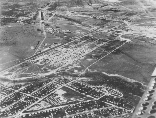
A U.S. Army camp near Townsville’s suburban areas, circa 1944.
By Tracy Cozzens
Beneath the surface of a tropical paradise in the city of Townsville on Australia’s Sunshine Coast lies a hidden maze of tunnels and underground bunkers, once said to be used by General Douglas MacArthur. Learning the secrets of this labyrinth that was a major World War II staging point for battles in the Southwest Pacific is the passion of Kevin Parkes of Geo Positioning Services, Townsville.
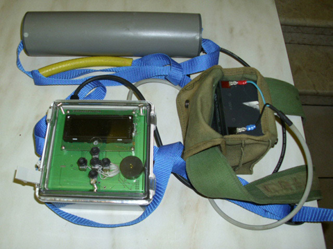
Parkes’ main tool is historic aerial photography, coupled with hours of research in the National Australian Archives and the National Library of Australia. To that he adds geophysical surveys of the infrastructure. Parkes is undertaking the geophysical surveying and mapping using an Ashtech ProMark 100 GNSS receiver and a Willy Bayot PPM Mk 3 magnetometer. He used the magnetometer and GPS receiver in parallel, later processing both data sets.
After the attack on Pearl Harbor and the Japanese advance through Asia, Townsville’s population bloomed from 30,000 to 120,000 by mid-1943. The rapid military influx stretched resources to the breaking point.
The U.S. Army 5th Air Force established the largest aircraft repair and maintenance facility ever built in the southern hemisphere at Townsville, and the site became the technical hub of U.S. military aviation. Air Force Service Command Depot #2 at Townsville was capable of overhauling 300 aircraft engines per month and performed aircraft assemblies, modifications, overhauls, and maintenance. Major resources and facilities serviced the Royal Australian Air Force, Australian and U.S. Armies, Royal Netherlands Air Force, Royal Air Force, Canadian forces, Royal Navy, and other allied forces.
“A visitor to Townsville today would be forgiven in asking where the artifacts of this massive military facility are today,” Parkes said. “There is very little remaining in any built structures that give any idea of what happened in this city 70 years ago.”
Parkes realized that underground cave shelters were most likely used for warehousing and storage, to keep stores out of the weather and protected from enemy action.
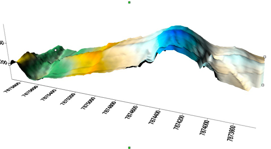
He describes one area he investigated, a park in Townsville used as an officer’s accommodation camp. Preliminary magnetic anomaly surveys indicated linear anomalies were beneath the park surface. A high-resolution survey gave samples of about 1.5-meter resolution.
“The difficulty was reducing all noise levels down to a minimum, including the X/Y positioning, so the GPS requirements came down to survey quality,” Parkes said. “It is absolutely critical that the GNSS receiver and magnetometer keep in synchronization during data collecting runs including under the frequently encountered tree canopies.”
To improve accuracy, Parkes avoids using real-time kinematic survey equipment. “That would involve having another electronic device operating and emitting more noise in the signal spectrum,” he said. The need to position the GPS antenna in close proximity to the magnetometer sensor was a major issue with all on-pole RTK systems.
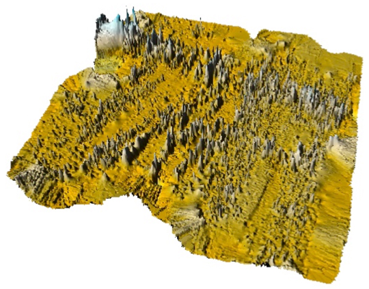
A U.S. Army air raid shelter under the officer’s accommodation camp, mapped with GPS and magnetometer data and using Surfer 3D surface mapping software.
With an Ashtech Promark 3, post-processed results were better than 100-millimeter X/Y coordinates. “The unit is lightweight and self-contained,” Parkes said. “The noise from the Ashtech survey-grade external antenna’s effect on the magnetometer data was insignificant.”
Still, this park had a grove of trees that defied every attempt to maintain GPS reception and consequently synchronize the magnetometer. Along came the Ashtech ProMark 100, a lightweight and self-contained receiver with external geodetic antenna with GPS and GLONASS. “My first attempt at surveying under the trees was spectacular to say the least,” Parkes said. “Synchronization with the magnetometer data was near perfect.”
The dual-constellation reception of the ProMark 100 became essential to the success of Parkes’ work. After more than a hundred data-collection passes with the magnetometer and ProMark 100 through the groves of trees, at no time did the Position Dilution of Precision (PDOP) rise to more than three, and at all times more than eight satellites were available. The ProMark 100 data is post-processed to improve accuracy. Parkes noted that ironically many of the most interesting finds have been collected under heavy tree canopy. Without the quality of the geographic positions enabled by the ProMark100 under tree canopy, Parkes said that much of his work would have been impossible to achieve.
Parkes’ surveying equipment includes a magnetometer and a ProMark 100 GNSS receiver.
In fact, when Parkes first began his mapping project in 2005, he used a single-constellation GPS system and post processed the results against the local International GNSS Service (IGS) reference station. The GPS-only system worked very well until a grove of trees would interfere with the sky. Now with the ProMark 100 GNSS receiver, Parkes surveys using GPS L1 and GLONASS in continuous kinematic mode at a one-second collection rate. He then post processes the data against another ProMark 100 used as a local reference station.
To date, Parkes has mapped an underground railway, artillery observation posts, several shelters, fuel terminals and other yet-to-be-identified pieces of the vast infrastructure.
During his Research, Parkes mapped a major magnetic anomaly in Cleveland Bay. In 1770 Captain James Cook in the HMS Endeavour mapped the east Australian coast. Venturing into Cleveland bay, Cook noticed his compass behaving erratically, and named one island Magnetic Island. Today, a 3D surface model reveals a large magnetic anomaly heading across Cleveland Bay and straight towards Magnetic Island, 7 kilometers from Townsville. Experts who have examined the data believe that it is a naturally occurring magnetic anomaly about 800 meters wide. “It would appear that Captain James Cook was indeed a very capable navigator and cartographer,” Parkes said.
A supersize bunch of pent-up GNSS just bust out all over. GLONASS is fully operational for the first time in more than 15 years. At least one Galileo in-orbit validation satellite broadcasts the new E1 and E5 signals, maybe both satellites by the time you read this. Compass has completed its regional navigation constellation. The first GPS III satellite testbed arrived at its integration and testing site in Colorado. The Russian SBAS is climbing back onto the air again. And QZSS has been quietly making progress, almost unnoticed.
For the first column since last February, I can write about something besides LightSquared.
Oops, I did it again.
But what a breath of sweet, fresh air.
Maybe now we can get back to the real business of this community: building systems, integrating sensors, exploring applications, and making the world a better place.
Can’t resist one last note about those creative financiers, now under Securities Exchange Commission investigation, over at LightSquared. A little bird overheard a certain someone say in mid-December, “I was at the FCC on Monday. The discussion was only about what happens after the LS bankruptcy. They are done with LS. This is all about positioning for litigation right now.”
Of course it’s not all over yet but the kicking and screaming. Companies have powerful lawyers and white houses have long tentacles into federal agencies.
Be that as it may, I promised to talk about GNSS, the whole GNSS, and nothing but the GNSS.
We, and by that I mean you, on three continents, are just kicking the milestones over. I’ve never seen a month in which so much progress was made on all fronts: GPS, GLONASS, Galileo, Compass, and QZSS. It has been my experience that a step forward for one system is often matched by a step back or at least sideways for another. It is after all a system of systems, and complex systems are by nature fraught with potential for temporary setback.
Knock on wood, interoperability moved further toward our grasp in the period November 28 to December 16, 2011, than during any other comparable span. We sometimes talk about a coming Golden Age of GNSS. We just witnessed the Golden Growth Spurt.
A brief note: With this issue, I assume the responsibilities of publisher of this magazine, as well as editor-in-chief. With colleagues Chris Litton (associate publisher, international account manager), the invaluable Tracy Cozzens (managing editor), and Charles Park (art director), we are collectively worth slightly south of three digits of GNSS experience. Count on us to keep a steady stream of business and technical news coming your way, and to keep this forum open for your views and opinons.
Across transportation, agriculture, industry, commerce, and finance, GPS has replaced earlier technologies, opened up innovative applications, and led to new ways of doing old things. GPS now plays a key role in the critical infrastructures of all industrialized nations, from the most sophisticated telecommunications system to the production of a simple loaf of bread.
Wheat is the world’s second staple food, and bread its main product. Bakers have been around for 30,000 years. GPS, among its manifold other duties, now also helps bring us our breakfast toast and midday sandwich.
British farmers sow 2 million hectares (5 million acres) of wheat per year, harvest 8 tonnes per hectare (3.6 U.S. tons per acre) and sell it at £150 a tonne ($214 per U.S. ton), making their harvest worth £2.5 billion ($3.9 billion). Nearly a billion pounds-worth ($1.6 billion) goes to make bread.
We use Britain as an example because we are British, but this same truth holds, at much grander scale, when you consider the United States, Russia, and many other European nations.
A vital value chain wends its way from farm to mill to bakery to store to home: in the UK, 99 percent of households buy bread, 99 percent of which is made in this country, 80 percent of it from domestic flour. This relatively closed value chain lets us see how GPS is used, and that its loss would increase the price of a loaf and translate into inflation.
GPS serves as the basis of the precision agriculture, cutting fuel costs and enabling selective and variable rate optimized application of fertilizers. It lets farmers use less manpower, reduces soil compaction, and even minimizes operator fatigue. Farmers now spend much more time on yield monitoring and within-paddock zone management than leaning on gates chewing straws. Though the capital cost of precision agriculture is high, the annual benefits are comparable with the investment. Losing GPS-based precision agriculture would increase the price of bread by at least 2 percent.
Transport logistics is the glue that joins our value chain together. GPS in fleet management optimizes routings, accelerates dispatching, prevents theft, improves driver behavior, and delivers fuel efficiencies. Loss of GPS in the transport links in our chain would increase fuel costs alone by 13 percent.
On top of all this, GPS is the ultimate source of precision timing supporting telecommunications links at every stage of the value chain, from wheat futures trading and banking transactions to voice, data, and Internet traffic.
The sudden loss of GPS in farming, transportation, communications, business management, and retail distribution, would substantially raise the price of bread, hit every household, and impact the national economy.
What applies to a traditional and at first glance low-technology product like bread applies across the board. The recent report on GNSS vulnerabilities by the Royal Academy of Engineering says that GPS and other satellite navigation services have applications so pervasive that there is now a real threat to global security if the systems should fail — or be interfered with. The signals are used by almost every industry: rail, road, aviation, space, maritime, agriculture, energy, surveying, construction, law enforcement and communications.
Dependence on GNSS connects many otherwise independent services into a so-called accidental system — with a single point of failure, the satellite signal. And a satellite signal, says the report, is a weak foundation for important services, since it can fail in dozens of ways.
GPS is no longer the only GNSS, of course, as many nations, recognizing its political and economic value, have developed their own systems, and augmentations to enhance accuracy and integrity. Over the next few years, the number of navigation satellites may approach 150. This will help reduce vulnerability to the loss of GPS and so will be a benefit in the short term.
But the long term is a very different matter. All these systems now use, or shortly will use, essentially the same technology. And, crucially, the same radio frequency bands.
In those frequency bands, GNSS is threatened by rising levels of radio interference. This threat has several strands that are being recognized separately and handled individually, but which taken together will determine the future of GNSS.
We face a Triple Whammy!
The First Threat
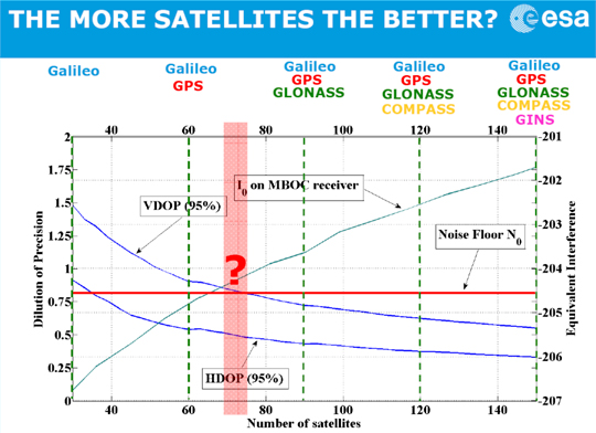
The first component of the Triple Whammy comes from the new satellite systems themselves. Each satellite transmitting in the GPS frequency band increases the noise level there. Satellite navigation receivers must find and lock onto the extremely weak signal that reaches the Earth, digging it out from the background noise of the cosmos. And the other GPS satellites add to the noise level.
Günther Hein of the European Space Agency shows this remarkable diagram (Figure 1): as the number of systems increases and the number of satellites heads for that 150, up rises the noise they make, the blue-green line. More than about 70 of them, and satellite noise exceeds the cosmic noise floor in red and becomes the main source of noise. The more satellites, the worse the reception as GNSS interferes with itself. Too many satellites, and you’d pick up none at all! The first threat of the triple whammy is self-inflicted.
Chart: David Last and Sally Basker
Figure 1. The first threat of the Triple Whammy: new satellite systems. Source: Günther Hein.
The Second Threat
Conflicts between nations as their new GNSSs compete for radio spectrum also threaten GNSS viability.
The frequency bands available to satellite navigation are essentially L2, L5, and the principal one we use currently, L1. On L1, the European Galileo system and the Chinese Compass system occupy the same areas. Now, that’s very desirable if the two systems are to share receivers. But they also compete for that spectrum, and there is conflict between Compass and Galileo.
This battle for spectrum is a highly complex engineering problem. But chiefly, the spectrum wars are political, even emotional.
Chinese satellites fly across American skies broadcasting signals that interfere with European receivers. Spectrum wars have everything to do with relationships between nations and little to do with battles between engineers. They are developing into a classic tragedy of the commons: a situation in which self-interest determines how a limited resource — here the radio spectrum — is to be shared in a regime in which regulation is weak. The International Telecommunication Union sets standards and registers claims. The UN Office for Outer Space Affairs seeks to mediate. But neither is a policeman; sovereign governments may sometimes be penniless, but they are very powerful.
The second threat of the Triple Whammy is also self-inflicted.
The Third Threat
Communications systems compete with GNSS for spectrum: witness the current LightSquared case of a powerful new broadband system. For existing receivers, including those in government systems and aviation, it seems there is no fix for its devastating interference. LightSquared is driven by rich and powerful commercial forces; it could well win this fight.
Communication technologies will continue to press upon the satellite navigation spectrum. LightSquared will likely erode spectrum gaps between communications and navigation services, the so-called guard bands.
Satellite navigation has become highly political. The intense use of GNSS across our economies makes them vulnerable. GNSS is threatened by a Triple Whammy, by jamming, and by spoofing. These increase the risks to our security and our economies, both in probability and impact. The solution of detecting jammers and making ownership illegal will help with local problems in local areas. But the Triple Whammy threats are not local; they are national and international, world-wide.
Today’s spectrum wars affect us all. That the loss of GPS would increase the price of a loaf — the very trigger for the French Revolution — brings this down to earth.
These are not technical issues, they determine the price of our food! They constitute a real and present danger to our societies — down to the mundane yet very real level of our daily bread.
David Last is a past-president of the Royal Institute of Navigation, a consultant and expert witness on radio-navigation and communications systems to companies, governmental and international organizations, and criminal investigators.
Sally Basker, former director of research and radionavigation at the General Lighthouse Authorities of the UK and Ireland, has opened Traxis Ltd: management, business, and technology advice with expertise in navigation service provision. See www.traxis.co.uk.
This article is adapted from a presentation at the European Navigation Conference, London, November 2011. A longer version of the talk appears in the Royal institute of Navigation News.
GALILEO PROTOFLIGHTMODEL satellite began transmitting E1 and E5 signals in early December. ESA reports them well within power and shape specifications, and suited for interoperability with GPS.
The Galileo ProtoFlightModel (PFM) in-orbit validation (IOV) satellite GSAT0101 began transmitting E1 signals on December 10 using the E11 ranging code, and E5 signals early on December 14. Launched at the same time, Flight Model 2 (FM2), GSAT0102, has not yet started transmitting navigation signals. Several companies and laboratories around the world immediately began processing the PFM signals. This story briefly aggregates their reports.
The European Space Agency (ESA) proudly released a statement: “Europe’s Galileo system has passed its latest milestone, transmitting its very first test navigation signal back to Earth. [. . . . ] The turn of Galileo’s main L-band (1200-1600 MHz) antenna came on the early morning of Saturday 10 December. A test signal was transmitted by the first Galileo satellite in the E1 band, which will be used for Galileo’s Open Service once the system begins operating in 2014. [. . . . ]
“The signal power and shape was well within specifications. The shape is especially important because its modulation is carefully designed to enable interoperability with the L1 band of U.S. GPS navigation satellites: Galileo and GPS can indeed work together as planned.
“The test campaign is concentrating on the first satellite for the reminder of the year, with the focus moving to the second Galileo satellite from the start of 2012. The plan is to complete In-Orbit Testing by next spring.
“The next pair of Galileo In-Orbit Validation satellites will also be launched next year, to form the operational nucleus of the full Galileo constellation. Meanwhile the next batch of Galileo satellites are currently being manufactured for launch in 2014.”
Thales Avionics. Thales Avionics has developed a Galileo receiver capable of processing the Open Service, Commercial Service, and Safety of Life service of the Galileo constellation.
Figure 1 shows a screenshot of the Thales Avionics receiver interface program, highlighting the L1 signal energy (top right) and the pilot secondary code (bottom). The satellite Doppler and C/N0 values have been recorded and are provided in Figure 2.
Figure 1. Screen of Thales Avionics receiver interface highlighting L1 signal energy (top right) and the pilot secondary code (bottom). (Click to enlarge).
Figure 2. Satellite doppler and C/N0 values from the Thales Avionics receiver.
Thales has developed a coherent processing of the Galileo E5 AltBOC(15,10) signal compatible with hardware architecture designed for independent processing of both E5a and E5b. This processing is fully compatible with the mismatch between the two RF channels on E5a and E5b, thanks to real-time calibration based on satellite signals. This processing only requires software implementation, without additional recurrent costs. The technique is relevant for future receivers operating in the E5 band, in order to significantly enhance the accuracy, with respect to thermal noise and multi-path, and to improve the cycle slip probability.
CONGO. Several COoperative Network for GIOVE Observation (CONGO) stations, including one at the University of New Brunswick, are tracking both the E1 and E5 signals. Figure 3 shows C/N0 values collected at UNB.
Figure 3. C/N0 values in dB-Hz of PFM 1-Hz data collected at the University of New Brunswick, on December 10. Time axis runs for 24 hours starting at 01:00 UTC. Receiver is a Javad Delta-G2T. JAVAD GNSS. On December 12, JAVAD GNSS announced that it has tracked the Galileo in-orbit validation satellite, temporarily designated PRN-11.
“An important point is that we tracked it with our units that are already in the market,” said Javad Ashjaee, CEO. “This is not a lab tests. Our customers can track it too.”
Figure 4 shows the company’s tracking results of PRN-11: plots of pseudorange (in chips), doppler (in Hz), and SNR (relative number).
Figure 4. JAVAD GNSS tracking results of Galileo PRN-11 for now, plots of pseudorange (in chips), doppler (in Hz), and SNR (relative number).
Calgary PLAN Group. The University of Calgary sent a detailed report. (See Figure 5 and next item.)
Figure 5. Raw correlator values for the E1 B/C, E5aI/Q and E5bI/Q signals. The bit periods can be clearly seen on E1B, E5aI and E5bI. The secondary code can be observed on E1C while the pilot signal can be seen on singals E5aQ and E5bQ. (From the Calgary Report.)
Galileo E1 and E5: the Calgary Report
By James T. Curran and Aiden Morrison
Researchers in the Position, Location and Navigation (PLAN) Group at the University of Calgary recorded E1 and E5 data using a single dual-channel front-end and subsequently acquired and tracked E1 B/C, E5a and E5b signals in the early morning of December 15.
Using a dual channel front-end designed in-house, a Novatel GPS-703-GGG antenna and a laptop computer, IF data was collected to examine these new signals. This data was processed by GSNRx, a reconfigurable a multi-system, multi-frequency software receiver developed by the PLAN Group.
At approximately 03:20 MST (UTC – 7:00) more than 20 GNSS satellites were visible from a rooftop mounted antenna. Having reconfigured the front-end to accommodate the E5 band, IF data was collected which included Galileo E1 B/C and E5 A/B, GIOVE-B E1 B/C and E5a, GPS L1 C/A and L5, and GLONASS L1 C/A. Following some last-minute modifications to GSNRx to include the Galileo E5b signals, the samples were processed, simultaneously tracking GPS and Galileo on both the L1/E1 and L5/E5 frequencies and GLONASS on L1.
A subset of the raw correlator values for the E1 B, E1 C, E5a I and E5a Q signals are shown in Figure 5 above. Note that the E1 C values have been offset by -2.0×10⁵ for clarity. A data-rate of 250 symbol/s is clearly visible on the E1 B and E5b signals while a 50 symbol/s stream can be observed on the E5a I signal. The 25 chip secondary code is also evident on E1 C at a rate of 250 chip/s.
All six components of the Galileo-PFM signals shown above (transmitted on PRN 11) were tracked independently and their signal modulations were found to agree with the Galileo Open Service ICD. A trace of the measured carrier-to-noise floor ratios for the Galileo signals is shown in Figure 6. As indicated by the ICD, the E5b signals were observed at 2 dB lower power than the E1 B and C signals. The E5a signals, however, were expected to be received at the same power as E5b and yet were observed at approximately 4 dB lower power. This is believed to be a combination of the antenna and IF filtering within the front-end as the E5a center frequency is located relatively near the pass-band edge of both. This front-end was initially designed for 40 MHz bandwidth, but used in this experiment at 50 MHz, as will be discussed later.
Figure 6. C/N0 for Galileo-PFM signals.
The software receiver was once again reconfigured, this time to produce signal correlator values spaced along a delay of approximately 700 m and 70 m for the E1 A/B and E5 A/B signals, respectively, such that the cross-correlation of the received and local-replica PRN sequences could be examined. The signals were tracked for 10 seconds and the 1 ms correlator values averaged, to produce estimates of the code cross-correlation function. The characteristic ripple of the CBOC modulation on E1 B/C can be seen in Figure 7 (left), particularly on the right-most ascending feature of the envelope. Likewise, the alt-BOC cross-correlation of E5a Q in Figure 7 (right) is as expected. It is noted that the E5a I signal has suffered some distortion due to the filtering effects mentioned above.
Figure 7. Measured cross-correlation functions for the Galileo PFM E1 B and C signals (left) and E5a I and E5b I signals (right).
For details of the PLAN group’s front-end, a flexible GNSS signal capture tool, and other specifics on the process employed, see the full-length article.
GPS III Testbed Sat Delivered
Lockheed Martin delivered the the GPS III Non-Flight Satellite Testbed (GNST), the program’s pathfinder spacecraft, to its Denver-area facility. The pathfinder will now undergo final assembly, integration, and test activities.
The GNST is a full-sized, flight equivalent prototype of a GPS III satellite used to identify and solve development issues prior to integration and test of the first space vehicle. According to the company, the approach reduces risk, improves production predictability, increases mission assurance and lowers overall program costs. In Denver, the GNST will be mated with its core structure, navigation payload, and antenna elements before completing pathfinding activities and checkout of environmental test facilities. The GNST will then be shipped to Cape Canaveral Air Force Station, Fla., for pathfinding activities at the launch site.
GPS III satellites, when launched as scheduled to being in 2014, will replace aging on-orbit GPS satellites to deliver better accuracy and improved anti-jamming power, while enhancing spacecraft design life and adding a new civil signal designed to be interoperable with international global navigation satellite systems.
In parallel with the GNST, progress on the first space vehicle is progressing on schedule. Lockheed Martin received the core structure for the first GPS III satellite in Stennis, Mississippi, on August 4, and is now integrating the space vehicle’s flight propulsion subsystem. The integrated core propulsion module will be shipped to the GPF in the summer of 2012 and will then undergo final assembly, integration and test in order to meet its planned 2014 launch.
The GPS III team is led by the GPS Directorate at the U.S. Air Force Space and Missile Systems Center. Lockheed Martin is the GPS III prime contractor with teammates ITT, General Dynamics, Infinity Systems Engineering, Honeywell, ATK and other subcontractors.
Drone Downed
Press reports speculate that GPS spoofing was used to get the RQ-170 Sentinel Drone to land in Iran. According to an Iranian engineer quoted in a Christian Science Monitor story, “By putting noise [jamming] on the communications, you force the bird into autopilot. This is where the bird loses its brain.” At that point, the drone relies on GPS signals to get home. By spoofing GPS, Iranian engineers were able to get the drone to “land on its own where we wanted it to, without having to crack the remote-control signals and communications.”
“The GPS navigation is the weakest point,” the Iranian engineer told the Monitor, giving a detailed description of Iran’s electronic ambush of the highly classified pilotless aircraft.
In 2011, the U.S. Air Force awarded two $47 million contracts to BAE Systems and Northrop Grumman for development of a navigation warfare sensor to replace military GPS receivers on aircraft and missiles, and designed to maintain freedom of action under extreme GPS countermeasures.
GLONASS Fully Operational
For the first time in more than 15 years, GLONASS is fully operational, with 24 satellites in their designated orbital slots, set healthy, and providing world coverage.
GLONASS 744, an M-class satellite and one of three launched from Baikonur on 4 November, was set healthy December 8, bringing the number of healthy operating satellites to the full complement of 24.
GLONASS briefly achieved a 24-satellite constellation in early 1996 but it degraded rapidly due to Russia’s economic difficulties following the break-up of the Soviet Union coupled with the short lifetime of the GLONASS satellites. Since 2002, the GLONASS constellation has slowly but surely been rebuilt with the Russian government’s commitment to provide a global positioning and navigation system comparable to that of GPS.
Luch SBAS. Roscosmos also launched the Luch-5A geostationary relay satellite on December 11.
Luch-5A is the first in a series of new data relay satellites designed to rebuild the Luch Multifunctional Space Relay System, which had ceased operating by 1998. Among other functions, 5A hosts a wideband satellite-based augmentation system (SBAS) transponder.
The SBAS transponder will transmit correction and integrity data for GLONASS and GPS on the GPS L1 frequency with a C/A pseudorandom noise code to be assigned by the GPS Directorate. The data will be provided by the System for Differential Correction and Monitoring or SDCM, which uses a ground network of monitoring stations on Russian territory as well as some overseas stations.
As the SDCM primary service area is Russian territory, the main lobe of the SBAS antenna beam will be directed to the north with an angle of 7 degrees relative to the direction to the equator. Transmitted power of 60 watts will give a signal power level at Earth’s surface roughly equal to that of GLONASS and GPS signals, about –158 dBW.
The current international SBAS data format has a limited capability for broadcasting corrections for both GLONASS and GPS satellites combined. There is space for only 51 satellites, insufficient for the current number of satellites on orbit. As a result, studies are being carried out in an attempt to resolve this problem. One option is to use a dynamic satellite mask, where an SDCM satellite would only broadcast corrections and integrity data for those GLONASS and GPS satellites in view of users in the territory of the Russian Federation.
Luch-5A is the first of three MSRS/SDCM satellites. Luch-5B will be launched in 2012 into a slot at 95 degrees east longitude and Luch-4, in 2014, into a slot at 167 degrees east longitude.
Beidou Launch Fills Regional Nav System
The Beidou-2/Compass IGSO-5 (fifth inclined geosynchonous orbit) satellite was launched on December. According to a Chinese government announcement, this launch completes the construction of the basic regional navigation system for service to China and will be operational by the end of the year. However, completion of the Phase II development, to provide service to the Asia/Pacific region, will require further satellite launches in 2012. Phase III global coverage, with a 30-satellite system, will be achieved by 2020 according to the Beidou website.
The GNSS community outside China still awaits a Compass interface control document (ICD), which has been promised by the end of 2012.
LightSquared Incompatibility Declared
U.S. government tests conducted in November showed that 75 percent of GPS receivers examined were interfered with at a distance of 100 meters from a LightSquared (LS)base station. The report states that “No additional testing is required to confirm harmful interference exists,” and “Immediate use of satellite service spectrum for terrestrial service not viable because of system engineering and integration challenges.”
The tests showed interference by the LS Low 10 terrestrial signal with an overwhelming majority of general-purpose GPS receivers. Data from LS handsets was collected, analysis is underway, but no results were given. Wideband and military receivers were tested, but neither specifications nor results were presented; a classified session was convened for that purpose.
Of the 92 receivers for which full data sets were compiled, 75 percent of them failed a 1db test, showing harmful interference at 100 meters from a LS base station. These 69 receivers failed at a broadcast level of around -15dBm from the LS transmitter.
In a December 7 filing with the FCC, LightSquared further revised its public plans to say that it would “limit its power on the ground when transmitting in the lower 10 MHz from 1526-1536 MHz to no more than –30 dBm until January 1, 2015, –27 dBm until January 1, 2017, and –24 dBm thereafter.” According to test data, at –30 dBm, approximately 17 percent of GPS receivers would be disrupted; at –27 dBm, 25 percent; at –24 dBm, 36 percent. Proceeding with this scenario would require the assumption that the FCC, or indeed anyone, believes anything that LightSquared says at any given instant, for any given duration.
By Ryan H. Mitch, Ryan C. Dougherty, Mark L. Psiaki, Steven P. Powell, Brady W. O’Hanlon, Jahshan A. Bhatti, and Todd E. Humphreys
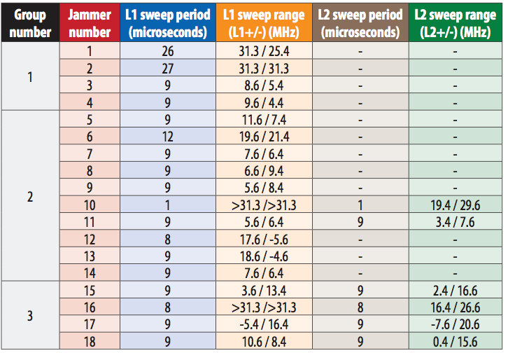
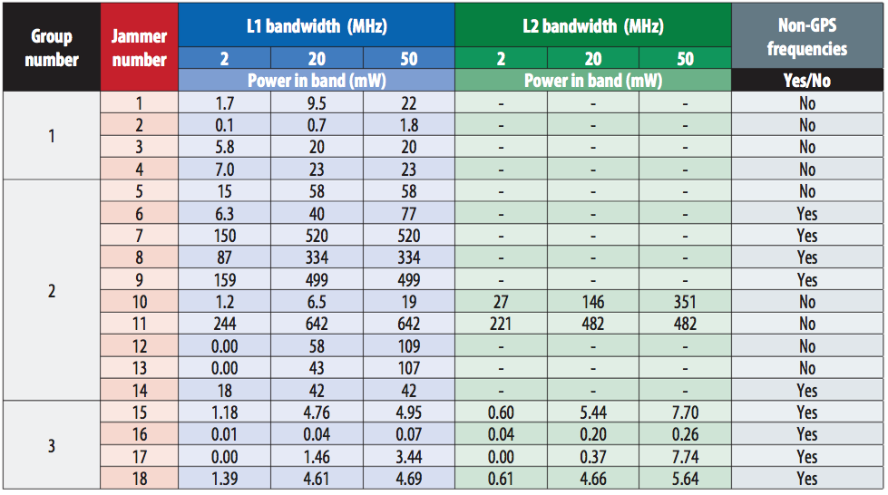
GPS jamming is a continuing threat. A detailed understanding of how the available jammers work is necessary to judge their effectiveness and limitations. A team of researchers from Cornell University and the University of Texas at Austin reports on their analyses of the signal properties of 18 commercially available GPS jammers.
INNOVATION INSIGHTS by Richard Langley
GPS IS AT WAR. It is a major asset for United States and allied military forces in a number of operating theaters around the world in both declared and undeclared conflicts. But GPS is at war on the domestic front, too — at war against a proliferation of jamming equipment being marketed to cause deliberate interference to GPS signals to prevent GPS receivers from computing positions to be locally stored or relayed via tracking networks.
There have been many notable examples of deliberate jamming of GPS receivers. Many more likely go undetected each day. In 2009, outages of a Federal Aviation Administration reference receiver at Newark Liberty International Airport close to the New Jersey Turnpike were traced to a $33, 200 milliwatt GPS jammer in a truck that passed the airport each day. The driver was reportedly arrested and charged. In July 2010, two truck thieves in Britain were jailed for 16 years. They used GPS jammers to prevent the trucks from being tracked after the thefts. And in Germany, some truck drivers have been using jammers to evade the country’s GPS-based road-toll system.
The U.S. and some foreign governments have enacted laws to prohibit the importation, marketing, sale or operation of these so-called personal privacy devices. Nevertheless, a certain number of jammers are in the hands of individuals around the world and they continue to be available from manufacturers and suppliers in certain countries. So, GPS jamming is a continuing threat both at home and abroad and a detailed understanding of how the available jammers work is necessary to judge their effectiveness and limitations. This information will also help in developing countermeasures that could be incorporated into GPS receivers to limit the impact of jammers.
Jammers constitute an enemy force, and as the Chinese General Sun Tzu stated in the Art of War more than 2,000 years ago, battles will be won by knowing your enemy. In the last verse of Chapter Three, he states:
So it is said that if you know your enemies and know yourself, you can win a hundred battles without a single loss.
If you only know yourself, but not your opponent, you may win or may lose.
If you know neither yourself nor your enemy, you will always endanger yourself.
In this month’s column, a team of researchers from Cornell University and the University of Texas at Austin reports on their analyses of the signal properties of 18 commercially available GPS jammers. The enemy has been exposed.
The Global Positioning System has become increasingly incorporated into civilian infrastructure. The increase in GPS-integrated systems has caused a proportional increase in the vulnerability of these systems to jamming and interference. The interests of individuals or groups willing to break the law may be served by interfering with the normal operation of GPS-enabled systems. As a result, in recent years many GPS jamming devices have become available for purchase over the Internet. These relatively cheap devices, some costing less than an inexpensive GPS receiver, pose a significant risk to the normal operation of many systems reliant on GPS.
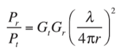
Many types of intentional radio frequency (RF) interference exist, including tones, swept waveforms, pulses, narrowband noise, and broadband noise. There are a number of methods for mitigating the effects of jamming and interference, and additional methods exist to locate the sources of the interference. Mitigation and location methods can be improved by use of a priori information about the interference source. This article provides such a priori information for a set of jammers and assesses their threats. Its results are based on two tests. The first test records raw RF data from a selection of jammers and analyzes it using fast Fourier transform (FFT) spectral methods. The second test evaluates the effective range of a subset of the GPS jammers using a commercial off-the-shelf (COTS) receiver.
The article presents results based on 18 civil GPS jammers. There are other types of GPS jammers for sale that were not tested. Furthermore, civil jammer behavior and design is likely to evolve over time. In this article, we draw conclusions based on only the jammers that we tested.
Overview of Civil GPS Jammers
Devices that claim to jam or “block” GPS signals are widely available through a number of websites and online entities. The cost of these devices ranges from a few tens of dollars to several hundred. Their price does not seem to correlate with the claims made by the purveyors of these devices regarding the features and effectiveness of the product in question. Effective ranges from a few meters to several tens of meters are advertised, but the actual effective ranges are significantly greater. Claimed and true power consumptions range from a fraction of a watt to several watts.
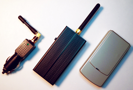
We grouped the GPS jammers we examined in this article into three categories based on morphology. The first is a group of jammers designed to plug into an automotive 12-volt auxiliary power supply outlet (cigarette lighter socket); this class of jammer is referred to in the remainder of this article as Group 1. The second category contains those jammers that are both powered by an internal rechargeable battery and that have an external antenna connected via an SMA connector; these jammers are referred to as Group 2. The jammers in Group 3 are disguised as cell phones; they have batteries but no external antennas. Figure 1 shows an example of a device from each of Groups 1–3.
Figure 1. Three jammers are depicted, from left to right Jammers 1, 5, and 15 from Groups 1, 2, and 3, respectively.
All 18 jammers broadcast power at or near the L1 carrier frequency, six broadcast power at or near the L2 carrier frequency, and none broadcast power at or near the L5 carrier frequency. Some of the jammers also broadcast power at frequencies outside of the GPS bands, typically cellular phone or Wi-Fi bands, but those frequencies are outside the scope of this article. Results in this article are for the current power levels broadcast in the GPS L1 and L2 bands, but examination of power levels in non-GPS bands indicate that many of these devices could be easily modified to broadcast much more power in the GPS bands.
The jammer antennas have been removed in most of the testing for this article, but their use in a real-world scenario will modify the jammer behavior. The antennas used by Group 1 and Group 2 jammers are loaded monopole antennas, while those used by the Group 3 jammers are electrically short helical antennas that have approximately the same gain pattern as the loaded monopoles. These antennas broadcast linearly polarized radiation, as opposed to the right-hand circular polarization of GPS signals. The polarization mismatch will cause some loss in received power at a right-hand circularly polarized GPS receiver antenna.
Jammer Signal Characteristics Test
The goal of the first set of tests was to record complex samples of the jamming signals and to derive the jammer characteristics from these data. A two-step procedure was used to collect useful data. The first step used a spectrum analyzer to find the frequency range of the jamming signal near L1 and L2. The second step used this frequency information to set the center frequency of a general-purpose RF digitization and signal storage device with a 12-drive RAID storage array. Offline analyses were then conducted on the recorded data.
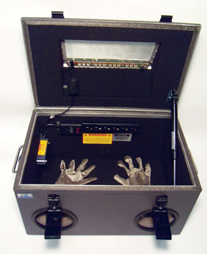
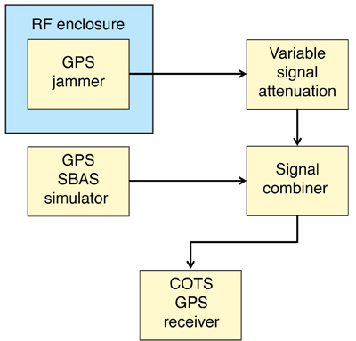
The test procedure was as follows. For the first two groups, the jammer was placed inside an RF-shielded test enclosure shown in Figure 2, to prevent any signal leakage, and its SMA signal output port was connected to the relevant data collection device using a shielded coaxial cable. The signal had to pass from the inside to the outside of the RF enclosure using the built-in coaxial feed-through. Note, therefore, that no jammer signal radiation occurred for Group 1 and 2 jammers even inside the RF enclosure. The enclosure was used primarily as a precaution.
Figure 2. RF-shielded test enclosure. Jammers were operated inside the enclosure to prevent emission of their RF signals.
None of the Group 3 jammers had external antennas. Therefore, they were allowed to radiate in the RF enclosure using their internal antennas. To capture the signal, a receiving patch antenna with active amplification was placed in the RF enclosure, and the antenna output was connected to the relevant RF recording device via the enclosure’s coaxial feed-through. The jammer and receiving antenna were separated by about 14 centimeters. The patch antenna field-of-view center was pointed directly at the jammer. The jammer was oriented such that the axis of its helical antenna was pointing perpendicular to the line from the receiving antenna to the jammer.
Jammer Signal Characteristics Test Results
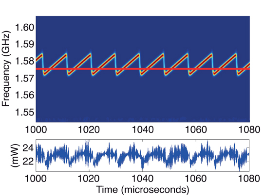
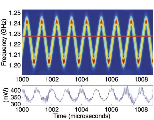
Although 18 jammers were tested, only a representative subset is discussed here. The signals were analyzed using FFT spectral methods and measurements of in-band power. Figure 3 displays the results of this analysis for a typical jammer from Group 1.
The top plot of Figure 3 graphs frequency on the vertical scale versus time on the horizontal scale. The bottom plot graphs power on the vertical scale versus time on the horizontal scale. Each vertical slice of the recorded RF data plot is a single FFT frequency spectrum. It covers 62.5 MHz centered on the L1 band and has a resolution of approximately 1 MHz. The relative power spectral density of each slice is indicated by color. The time axes of both plots span 80 microseconds.
Figure 3. Jammer 4 power spectral density versus time, with color indicating relative power (top plot) and power versus time in a 62.5-MHz band centered at the L1 carrier frequency (bottom plot).
The upper plot of Figure 3 is clearly that of a linear frequency modulation interspersed with rapid resets — a series of linear chirps. Each sweep takes nine microseconds and spans a range of about 14 MHz. This range includes the civil L1 GPS band. The center frequency is depicted by the horizontal red line in the top plot. The power is about 20 milliwatts and remains fairly constant over the sweep.
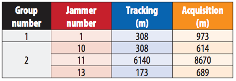
Three of the Group 1 jammers appeared to be of the same model and one was slightly different. All of them broadcast power only at L1. Despite their similarities in external appearance, the three jammers of the same model exhibited markedly different signal properties. These differences will be presented later in terms of tabulated frequency modulation characteristics and in-band power levels.
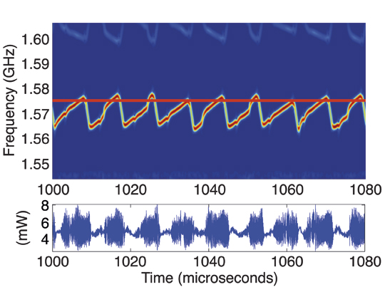
One of the Group 2 jammers was unusual in two respects, as illustrated in Figure 4. This figure plots the L2 spectrum whose center is indicated by the horizontal red line in the top plot. The first obvious difference from Figure 3 is that the frequency modulation in time is a triangular wave instead of a sawtooth. Additionally, the modulation frequency is very high in comparison to all the other jammers; its period is only about 1 microsecond. Note that the horizontal scale of this figure spans only 8 microseconds, that is, 10 times less than in Figure 3.
The other Group 2 jammers tended to broadcast sawtooth frequency modulations as in Figure 3. They all broadcast jamming power at L1. Of course, the jammer depicted in Figure 4 broadcast power at L2 as well. Only one other Group 2 jammer had L2 jamming capability. Two of the jammers suffered from poor design of their L1 frequency modulation schemes: they placed no jamming power closer than 4.6 MHz away from the nominal L1 carrier frequency.
Figure 4. Jammer 10 power spectral density versus time (top plot), with resolution of about 3 MHz and color indicating relative power, and power versus time (bottom plot) in a 62.5-MHz band centered at the L2 carrier frequency.
Another unusual frequency modulation was encountered in a Group 3 jammer. The L1 results for this jammer are depicted in Figure 5. It seems to show a linear-type frequency modulation distorted by sudden frequency jumps, as seen in the upper plot of the figure. Despite its irregular nature, this waveform maintains its jamming efficacy.
Figure 5. Jammer 15 power spectral density versus time, with color indicating relative power (top plot) and power versus time in a 62.5-MHz band centered at the L1 carrier frequency (bottom plot). Note the additional frequency jumps in the sweep pattern.
All four jammers in Group 3 broadcast power at L1, L2, and additional frequency bands. Three of the jammers appeared to be of the same model, while a fourth was different. Jammers in this group normally use a standard sawtooth frequency modulation. Figure 5 represents the exception.
Additional types of distortion from the nominal sawtooth frequency modulation have been observed in some of the jammers. Discussion of each additional variation has been omitted here for the sake of brevity. See the authors’ companion conference paper, listed in the Further Reading sidebar for more details.
Frequency Modulation Periods and Ranges. The frequency modulation characteristics of all 18 jammers are listed in Table 1. The first two columns identify each jammer by group number and jammer number. The sweep period and frequency range for the L1 sweep are shown in the third and fourth columns. The two numbers in the fourth column are the upper and lower bounds of the jamming tone sweep range in megahertz above and below the L1 carrier frequency. For instance, the period between resets of the linear frequency modulation of Jammer 1 is 26 microseconds and the tone sweeps from 25.4 MHz below L1 to 31.3 MHz above L1. The fifth and sixth columns are analogous to the third and fourth columns, but for jamming in the L2 band, with entries only for those jammers that broadcast in this band.
The sweep periods were calculated using four contiguous sweeps from near the beginning of each data set and another four sweeps 30 seconds later. The sweep periods exhibited standard deviations of less than 1 microsecond. The reported sweep ranges are the minimum and maximum frequency observed in the same data used to calculate sweep periods. The sweep ranges changed by as much as 2.5 MHz between sweeps.
One can make a number of observations based on Table 1. First, as mentioned previously, jammers which appeared to be of the same model exhibited significant variations in sweep behavior. For instance, Jammers 1, 3, and 4 appeared to be of the same models, yet Jammer 1 has a sweep period nearly three times as long as Jammers 3 and 4. It also has a sweep range four times as wide. Second, some individual jammers were exceptional. For example, Jammer 10 has a sweep period nearly 10 times shorter than any other jammer, and its L1 sweep range exceeded the 62.5 MHz bandwidth recorded by the RF sampling equipment. The sweep range of Jammer 16 also exceeded the sampled bandwidth, though its sweep period was not exceptional. Jammers 12 and 13 do not sweep through the L1 carrier frequency, as indicated by the negative signs in the fourth column of Table 1. Jammer 17 suffered from the same problem, but for both L1 and L2.
Table 1. Frequency characteristics of GPS jammers.
In-Band Jammer Power Levels. The GPS signal is spread over several megahertz by the pseudorandom noise (PRN) codes that modulate the L1 or L2 carrier waves. Different GPS receivers exploit this spreading by processing more or less of the full bandwidth. The RF power of the GPS jamming signal within different bands centered at L1 is an important concern because different receiver RF front-end bandwidths may allow different total amounts of jammer power to pass through them. For example, a C/A-code receiver with a 2-MHz RF front-end bandwidth will pass 10 dB less jammer power than will a 20-MHz bandwidth RF front end of a P(Y)-code receiver if the jammer in question spreads its power evenly over the 20-MHz band centered at the L1 carrier frequency. If the jammer power is concentrated in a 2-MHz range, however, then both receiver front ends will pass equal total jammer power.
To determine the power in different bandwidths, the raw data were filtered to pass only the bandwidths of interest. The data were digitally filtered using a finite input response (FIR) equiripple band-pass filter, providing 60 dB of attenuation at 2 MHz past the roll-off frequency. Note that a real GPS receiver will probably not have analog filter frequency roll offs as sharp as those used in our work.
Table 2 presents the results of this study. It reports power measurements averaged over 15 milliseconds in three different bandwidths: 2, 20, and 50 MHz, all centered at the nominal L1 or L2 carrier frequency. The table also indicates whether each jammer broadcasts power at frequencies other than the GPS frequencies. No power data is given for the non-GPS frequencies because they are not the focus of this article.
A number of observations can be drawn from Table 2. First, there is a large variation in broadcast power among jammers, with Group 2 jammers being on average more powerful. Specifically, Jammer 11 is the most powerful, broadcasting more than a watt in the GPS bands! Second, jammers of the same model broadcast roughly the same amount of power despite the differences in sweep behavior mentioned above. For instance, Jammers 1, 3, and 4 broadcast roughly the same amount of power, and Jammers 15, 17, and 18 do so as well. Third, the poor frequency plans of Jammers 12, 13, and 17 are apparent in the power measurements. These jammers did not sweep a tone through L1 or L2, and effectively no power was measured in the 2-MHz band centered on the L1 or L2 carrier frequencies.
Table 2. Jammer power levels in frequency bands of interest.
Although not shown in the tables, Jammers 12, 13, and 14 exhibited periodic variations in broadcast power. Their peak-to-peak power varies as a sawtooth wave with period approximately 15 milliseconds and amplitude on the order of 10 percent of the total broadcast power.
The measured power values in Table 2 for jammers of Groups 1 and 2 were derived using direct cable connections. Thus, they report the total power into the transmitting antenna. The power received at a GPS receiver’s RF front end will be affected by any antenna inefficiency, the antenna gain pattern, and the space loss, among other effects.
In contrast, the power reported for Group 3 jammers includes all of those effects for the given test configuration. Specifically, the receiving antenna picked up only a fraction of the radiated power because the receiving antenna subtended only a fraction of the 4π steradians around the transmitting antenna. Also, the power that was received was boosted by the receiving antenna’s active low-noise amplifier. Finally, the radiation environment inside the RF enclosure is uncertain, and the enclosure constrains the separation of the antennas to be on the order of one wavelength, thereby giving rise to near-field effects. Therefore, the indicated power levels for the Group 3 jammers do not constitute measures of absolute power. The tabulated power levels for Group 3 jammers are included primarily for purposes of comparison within the group.
Maximum Effective Range Test
The goal of the second set of tests was to determine the effective ranges of the GPS jammers when interfering with a COTS receiver. A constraint on this test was that it could not broadcast harmful radiation to the environment. Ideally, the jammers and a receiver would be taken outside and tested with all antennas attached. However, this type of test would possibly interfere with other equipment and is illegal in the United States. A close approximation to this scenario can be constructed using a high-fidelity simulated GPS signal, a commercial GPS receiver, a GPS jammer in an RF enclosure, and a set of attenuators to simulate various distances. The setup for the second test is shown in the block diagram of Figure 6.
Figure 6. Block diagram of the test procedure and equipment used to determine the GPS jammers’ effective ranges.
Each range test involved running a GPS jammer inside the RF enclosure, passing its signal through the enclosure’s coaxial feed-through, and electrically combining that signal with a GPS simulator signal. The combined signal was then input to the antenna connector of the COTS GPS receiver. Attenuators were inserted in-line with the GPS jammer before it arrived at the combiner. Using this setup, two tests were conducted. The first test determined the jamming signal attenuation level necessary for continuous tacking. The second test determined the attenuation level necessary to allow the receiver to acquire the simulator signal within five minutes from a cold start. As will be shown in the next section, the resulting attenuation values can be converted into effective ranges of the jammers if one makes certain reasonable assumptions about transmitting and receiving antenna gains and path losses.
The simulator power level was set so that the power into the receiver matched that which it would receive from the actual GPS constellation through a typical roof-mounted passive patch antenna. This power level was checked by comparing the resulting C/N0 for all of the visible satellites when using the simulator against typical C/N0 values when using the roof-mounted antenna. Typical levels reported by the receiver were C/N0 = 43 dB-Hz.
Maximum Effective Range Results
The jamming signal attenuation levels resulting from the two tests are presented in Table 3. These tests were conducted on one jammer from Group 1 and three jammers from Group 2. No jammers from Group 3 were included because of the broadcast power uncertainties discussed in connection with Table 2.
The attenuation values by themselves are not very useful, but they can be converted into distance measurements with a number of assumptions. The ratio of received power to transmitted power can be expressed as
where Gt is the transmitting antenna gain, Gr is the receiving antenna gain, and the term (λ/(4πr))2 is the path loss for radiation of wavelength λ over the distance r. This equation can be solved for the range, r:
The quantity in this formula that equates to the total electrical jammer attenuation produced in each bench-top test is the product of the antenna gains and the ratio of transmitted to received power: Gt Gr(Pt ⁄Pr ).
To convert the results in Table 3 into effective ranges, the transmitting and receiving antennas can be assumed to be perfect, lossless, isotropic radiators. In this case, the gain terms, Gt and Gr , are unity. Each measured attenuation value can be converted to the unitless ratio, Pt ⁄Pr , and substituted into the equation for r. Use of this equation at the L1 carrier frequency yields the ranges in Table 4. If the range between the jammer and receiver is less than that listed in the third column of the table, then the jammer will prevent the receiver from tracking and acquiring. If the range is less than that listed in the last column but more than that listed in the third column, the receiver will continue to track but be unable to acquire. The effective ranges are at least an order of magnitude greater than the claims of the jammers’ purveyors.
Table 3. Jammer attenuation levels needed to allow COTS GPS receiver acquisition and tracking.Table 4. Ranges of jammer effectiveness against COTS GPS receiver when using lossless isotropic antennas.
Distinct scenarios with different antennas can be approximately tested using Table 3 and the range equation. For example, a patch antenna that is oriented perfectly skyward might have 10 dB of attenuation at very low elevation angles, and the jammer might have an additional 3 dB loss due to polarization mismatch. In this scenario, the effective jamming range would be factored down by 10-13/20 = 0.22. In this case, Jammer 11’s tracking interference range would be reduced from 6.1 kilometers to 1.4 kilometers. Additional jammer signal attenuation might occur if the emissions passed through the reduced RF aperture of a vehicle’s body and windows. Such an effect could be incorporated into the range equation to determine a revised effective range.
Due to the ignored losses in the real system, it would likely be safe to assume that the effective ranges of the GPS jammers would be no greater than those listed in Table 4. The ranges could potentially be greater if a high-gain receiving antenna were aimed directly at the jamming source, or if the jamming source used a high-gain transmitting antenna aimed at the receiver. None of the jammers tested employed such an antenna.
Summary and Conclusions
This article has presented the signal properties of 18 commercially available GPS jammers as determined from two types of live experimental tests. The first test examined the frequency structures and power levels of the jammer signals. It showed that all of the jammers used some sort of swept tone method to generate broadband interference. The majority of the jammers used linear chirp signals, all jammed L1, only six jammed L2, and none jammed L5. The sweep period of the jammers is about 9 microseconds on average, and they tend to sweep a range of less than 20 MHz. Some of the jammers’ sweep ranges failed to encompass the target L1 or L2 carrier frequencies.
The second test provided an estimate of four of the jammers’ effective ranges when deployed against a typical commercial receiver. An upper bound on the effective ranges was calculated for idealized, lossless, isotropic radiating and receiving antennas with matched polarizations. The weakest of the four jammers affected tracking at a range of about 300 meters and acquisition at about 600 meters, while the strongest affected tracking at a range of about 6 kilometers and acquisition at about 8.5 kilometers.
Acknowledgments
The authors thank the U.S. Department of Homeland Security for providing interference devices for testing. This article is based on the paper “Signal Characteristics of Civil GPS Jammers” presented at ION GNSS 2011, the 24th International Technical Meeting of the Satellite Division of The Institute of Navigation, Portland, Oregon, September 19–23, 2011, where it received a best-presentation-in-session award.
Manufacturers
The tests discussed in this article used an Agilent Technologies (www.home.agilent.com) model N1996A spectrum analyzer, a National Instruments PXI-5663 RF vector signal analyzer, a Ramsey Electronics model STE3000B RF shielded test enclosure, an Antcom (www.antcom.com) model 53G1215A-XT-1 patch antenna, and a NovAtel ProPakII-RT2 GPS receiver.
Ryan H. Mitch is a graduate student in the Sibley School of Mechanical and Aerospace Engineering at Cornell University, Ithaca, New York. He received his B.S. degree in mechanical engineering from the University of Pittsburgh.
Ryan C. Dougherty is a graduate student in the Sibley School. He holds a B.S. degree in aerospace engineering from the University of Southern California.
Mark L. Psiaki is a professor in the Sibley School. He received a B.A. degree in physics and M.A. and Ph.D. degrees in mechanical and aerospace engineering from Princeton University.
Steven P. Powell is a senior engineer with the GPS and Ionospheric Studies Research Group in the Department of Electrical and Computer Engineering at Cornell University. He has M.S. and B.S. degrees in electrical engineering from Cornell University.
Brady W. O’Hanlon is a graduate student in the School of Electrical and Computer Engineering at Cornell University. He received a B.S. degree in electrical and computer engineering from Cornell University.
Jahshan A. Bhatti is pursuing a Ph.D. degree in the Department of Aerospace Engineering and Engineering Mechanics at the University of Texas (UT) at Austin, where he also received his M.S. and B.S. degrees. He is a member of the UT Radionavigation Laboratory.
Todd E. Humphreys is an assistant professor in the Department of Aerospace Engineering and Engineering Mechanics at UT Austin and Director of the UT Radionavigation Laboratory. He received B.S. and M.S. degrees in electrical and computer engineering from Utah State University and a Ph.D. degree in aerospace engineering from Cornell University.
Further Reading
• Authors’ Conference Paper
“Signal Characteristics of Civil GPS Jammers” by R.H. Mitch, R.C. Dougherty, M.L. Psiaki, S.P. Powell, B.W. O’Hanlon, J.A. Bhatti, and T.E. Humphreys in Proceedings of ION GNSS 2011, the 24th International Technical Meeting of The Satellite Division of the Institute of Navigation, Portland, Oregon, September 19–23, 2011, pp. 1907–1919.
“Car Jammers: Interference Analysis” by R. Bauernfeind, T. Kraus, D. Dötterböck, B. Eissfeller, E. Löhnert, and E. Wittmann in GPS World, Vol. 22, No. 10, October 2011, pp. 28–35.
“GPS Jamming: No Jam Tomorrow” in The Economist, Technology Quarterly Special Section, Vol. 398, Issue 8724, March 12, 2011, pp. 20–21.
Modern Communications Jamming Principles and Techniques, 2nd ed., by R.A. Poisel, published by Artech House, Boston, Massachusetts, 2011.
“Jamming GPS: Susceptibility of Some Civil GPS Receivers” by B. Forssell and R.B. Olsen in GPS World, Vol. 14, No. 1, January 2003, pp. 54–58.
“A Growing Concern: Radiofrequency Interference and GPS” by F. Butsch in GPS World, Vol. 13, No. 10, October 2002, pp. 40–50.
“Interference Effects and Mitigation Techniques” by J.J. Spilker Jr. and F.D. Natali, Chapter 20 in Global Positioning System: Theory and Applications, Volume I, published by the American Institute of Aeronautics and Astronautics, Inc., Washington, D.C., 1996, pp. 717–771.
• Government Regulations and Actions Against Jammers
“The Civilian Battlefield: Protecting GNSS Receivers from Interference and Jamming” by M. Jones in Inside GNSS, Vol. 6, No. 2, March/April 2011, pp. 40–49.