Sometimes a market niche appears to be heading toward better things — even if the economy is not. This year’s Transportation Research Board’s Annual Meeting had its highest attendance ever. While intelligent transportation systems meetings have been shunned in the last few years as being too government-focused, some forward-thinking companies are using the Washington, D.C.-based meeting as a springboard for their enterprise location-based services offerings.
WASHINGTON — While enterprise and government markets are not as sexy as traditional friend-finding location-based services, a lot can be said about companies trying to make inroads in this developing marketplace. At the recent Transportation Research Board Annual Meeting here, such companies as TomTom are leveraging its community input options from its consumer navigation devices and map-building to government and enterprise markets.
While saying the portable navigation device will endure for a long time — and will never disappear — Maarten van Gool, TomTom’s Licensing Business Unit managing director, said that the company is looking at providing navigation and location products on multiple platforms. “For decades, we have delivered location and map content to the government and enterprise markets and we work with such companies as ESRI and Pitney Bowes Business Insight and federal, state, and local government agencies,” he said.
Van Gool said that government experts and policy-makers need detailed and reliable decision-making support tools to make timely and cost-effective decisions on changes to their local traffic management programs. “The intelligent transportation systems market can benefit from accurate and comprehensive information about travel times, traffic speeds, local accessibility, and travel patterns, which are the basic building blocks for forming cohesive traffic management plans,” he said.
Also at TRB last month, TomTom announced a partnership with PTV where PTV will be able to deliver TomTom traffic content, via TomTom Traffic Stats, to its customers in the transportation sector. “We are really only at the beginning of what we can offer and we look forward to delivering additional products for the government and enterprise markets based upon our vast historical traffic database and real-time traffic capabilities; these will become available over the course of 2011,” van Gool said. “The total [government] market size is yet to be quantified, and as the technology innovation in this space expands, we are on track to support it. We believe we can revolutionize traffic information by utilizing our assets and capabilities and we are working to educate the market before its full potential is reached.”
In other TomTom news, if you haven’t seen it already, it looks as if the company is phasing out the Tele Atlas name at trade shows. Most company personnel are now wearing TomTom badges during this transition.
In one of the big TRB announcements, the U.S. Department of Transportation’s Research and Innovative Technology Administration announced the Connected Vehicle Technology Challenge. The new competition seeks industry ideas for using wireless connectivity between vehicles.
RITA, through the competition, is soliciting ideas for products or applications that use dedicated short-range communications, which will be the basis for a future system of connected vehicles that will communicate with each other as well as the surrounding infrastructure, such as traffic signals, work zones and toll booths.
According to a National Highway Traffic Safety Administration report, wireless vehicle-to-vehicle (V2V) and vehicle-to-infrastructure (V2I) communications can potentially address 81 percent of all unimpaired vehicle crashes. Selected prize recipients will be fully funded to present their ideas for connected vehicle technology.
The competition, which runs through May 1, is open to all companies, not just those involved in transportation. More information can be found at www.challenge.gov.
Qualcomm Makes LBS News with Neer
Concentrating on privacy as a market driver, Neer, which is a subsidiary of Qualcomm Services Labs, allows a users to determine where, when, and who their location information is sent to. The company says applications include not only allowing family members to know where a loved one is, but business users to schedule information to co-workers.
Privacy is what Neer, which had a strong presence in the Qualcomm booth at last month’s Consumer Electronics Show, hopes separates it from the Foursquare, Gowalla, Twitter, and Facebook Places of the world.
“First and foremost, Neer was not designed to broadcast your location to vast numbers of people. Instead, Neer allows you to selectively choose the people, places, and times you are comfortable sharing your location,” said Ian Heidt, Neer director of services strategy. “And because we enable private sharing only with those you are most close to, we have seen growing acceptance of sharing places such as one’s home or work, places that have typically been taboo in other apps. We also wanted Neer to fit in more naturally with how people behave, so Neer works simply, securely, and automatically — there is no need to ‘check in’ like other apps. And because we believe that people want to keep this information securely within their control, there are no means to share location outside Neer.”
Right now, Heidt said that Neer is free, with no charges or advertising. “In the future, we may explore ways of including relevant ads, but for now, it is totally free on both Android and iPhone,” he said. “We are looking into numerous ways that we can monetize Neer by connecting people to the places they go. But in all cases, our primary goal is to preserve the trust that Neer is both helpful to your day and under your control.”
It’s easy to jump ahead and talk about the exciting things happening today and on the horizon in the geospatial industry. Rich 3D visualizations, complex databases, sophisticated analysis, high-tech data collection equipment, etc. But what about the thousands, maybe hundreds of thousands, of people who could benefit from just being able to take the first step of importing basic information and coordinates into a mapping program.
Last week, a reader sent me a small dataset of simple lat/lon coordinates in Excel and asked me the best way to import them into some sort of mapping software. My first inclination was to use ArcGIS.com or Google Earth, or something online to avoid having to download, install and maintain software on local computers. But alas, that was not to be. After a quick post to the ArcGIS Resource Center Forum, I quickly found out that ArcGIS.com was not going to work.
“Nelson” responded to my post with the following:
Hey Eric,
Unfortunately, there is no direct way to add layers, csv files, etc., to ArcGIS.com; however, Esri has noted on a couple of occasions that they are exploring the possibility of this functionality.
Hmmm….I briefly considered Google Earth, but my experience has not been great with Earth or Earth Pro. It’s ok, but still a little cheesy for my tasted.
When I suggested that my back-up plan was to investigate ArcGIS Explorer, Nelson responded:
ArcExplorer is definately the route you should take.
There are a number of advantages to it:
1) The points can be imported very easily using the GUI.
2) If they ever do decide to shift to a GIS, the layers in ArcExplorer can be shared using Layer Packages or KML files.
3) The Google Earth interface is not as user friendly as ArcExplorer and you also have the ability to change to a number of Basemaps on the fly — ArcGIS Online (Imagery, Topographic, Streets) Bing and OpenStreetMap with 2D/3D rendering.
Lastly, if you yourself are an ArcGIS user, it will probably make your life a little bit easier to work with a format that is well organized and familiar to you.
Cheers,
P.S. At the Federal User Conference, Esri announced there is going to be tons more functionality built in to ArcExplorer over the course of the year.
At that point, I committed to trying ArcGIS Explorer. Please note that I’m the last person to open a manual for this kind of software. I really think it should be straight-forward enough to figure it out in a few minutes. The only reference I used was the online ArcGIS Explorer Desktop FAQ and I accessed the Help file once. Of course, I used the ArcGIS Explorer Forum, which is very good.
Here is a screenshot of the data I had to work with. it was 62 records long, a subset of the actual dataset.
I spent the most time making sure the coordinates were formatted correctly. The original spreadsheet had N/S/E/W to indicators instead of positive and negative. For example, instead of -17 04.201, it was formatted as 17 04.201s, with the “s” denoting south latitude. For your reference, north latitude is positive values, south latitude is negative, east longitude is positive, and west longitude is negative. This had to change. With only 62 records, I could do it by hand in a couple of minutes. If I had to change 600 or 6,000 records, I would have used a more automated method.
The other item I needed to figure out were the attributes. None were provided in the spreadsheet, so I inserted a description number and a title for each point.
Once the spreadsheet was formatted correctly, the rest was very quick and straight-forward. After installing ArcGIS Explorer, this is what you see when you run the program.
If any of you had used ArcExplorer in years past like I did, this is totally different, and refreshing.
I saved the Excel spreadsheet as a CSV file (Comma-delimited text file).
To import into ArcGIS Explorer, simply select Add Content/Text Files.
Once you select the CSV file, it reminds me of importing a CSV file into Excel in that you have to define what each spreadsheet column means, although ArcGIS Explorer does recognize some of the fields automatically. For example, if the top of a column is labeled lat, latitude, y, y-coord, y-coordinate, ArcGIS Explorer automatically assumes the data in the column contains latitude data. The same goes for the longitude and elevation fields. For a good description of importing text files, click here.
First text import screen:
Second text import screen:
After clicking on Finish, the data is imported and displayed in ArcGIS Explorer.
The background imagery is automatically displayed and there are a number of display and analysis options.
To query a particular feature, simply click on it. A window is displayed as follows:
The pop-up window could display a number of things such as hyperlinks, photos, videos, etc.
Once your data is imported, other map data can be added to customize the final to your liking.
Finally, there is a 3D view that I tried, but it didn’t work for me. I suspect it had to do with my laptop video card or video memory, but I would like to have seen it work. That would have been cool to see, especially if a rough terrain surface was visible.
Alas, there is an online version of ArcGIS Explorer I didn’t try. There was some discussion about it at the 2011 Esri Federal User Conference (FedUC) a couple of weeks ago. Click here to see what’s coming in future updates of ArcGIS Explorer Online.
Thanks, and see you next week.
<
span style=”font-size: 11px; color: rgb(82, 82, 82); line-height: 16px; font-family: Arial;”>Follow me on Twitter at http://twitter.com/GPSGIS_Eric
On April 2, German Federal Minister of Transport, Building and Urban Development Peter Ramsauer will officially open the German Galileo test and development infrastructure GATE with the operator IFEN GmbH. The official opening will be carried out in the presence of the operator of GATE, IFEN GmbH, and guests.
GATE has now completed its signal upgrade phase, according to the latest version of the ESA Galileo Signal-In-Space (SIS) Interface Control Document (ICD) and the European GNSS Agency (GSA) Public Galileo Open Service (OS) ICD after successful final acceptance by the German Space Agency of the DLR at the end of November 2010.
The GATE test infrastructure is now capable of transmitting the Galileo OS, the Galileo Safety-of-Life (SoL) Service (functional), the Galileo Commercial Service (CS), and a Galileo Public Regulated Service (PRS) dummy signal.
The GATE system upgrade has been further extended to also support user integrity testing. GATE is now capable of simulating simple feared events on system/satellite level, so that the GATE system will support GPS and GATE/Galileo dual constellation RAIM, individual user integrity test scenarios as well as test of receivers with different RAIM functionalities.
The next step will be the aspired certification of the GATE test infrastructure as an officially accredited open-air test infra- structure to perform the necessary tests needed for the certification process to certify Galileo SoL equipment.
Using the Augmentation System with GPS-Equipped Mobile Phones
By François Boullete, Boris Kennes, Michaël Mastier, and Lee Banfield
GPS corrections from the European Geostationary Navigation Overlay Service can improve the positioning accuracy and user experience of GPS-enabled mobile phones, even if EGNOS satellites are not visible and even when the GNSS chipset in the phone does not support satellite-based augmentation systems.
Today, more than 20 percent of mobile phones in use in Europe include a GNSS chipset, and the penetration is expected to exceed 50 percent in the next 5 years. Despite its success in other sectors such as agriculture since the launch of its Open Service in October 2009,
EGNOS has received limited adoption in location-based services (LBS) and consumer applications, due to two main obstacles. First, the signals from the three EGNOS geostationary satellites that are easily received in open-sky environments are difficult to receive in cities, due to masking by buildings. Second, most GNSS chipsets embedded in today’s mobile phones are GPS-only without SBAS support, or use SBAS for ranging only, a function not supported by EGNOS at this stage.
The European GNSS Agency (GSA) and the European Commission (EC) supported the work described here to provide mobile phone operating system and application developers with a library of functions to allow them to benefit from EGNOS in all their applications. It works by receiving correction data via mobile communication networks when EGNOS satellites are not visible to the user device and even when using a standard GPS chipset, overcoming these two main obstacles for adoption.
Targeted mobile operating systems now include Nokia Maemo, Google Android, and Microsoft WinMobile. Further work will extend to this list to other compatible platforms.
This article demonstrates the feasibility and shows the performance of a software-based EGNOS solution and seeks to create awareness among mobile operating system and application developers on EGNOS.
User Benefits and Constraints
Although the sources of GPS positioning errors in urban areas are mainly due to multipath and GPS satellites availability, SBAS corrections on GPS satellites clocks and orbits and ionospheric correction model can still add value in case of moderate multipath environment characteristics. Although GPS stand-alone accuracy is nowadays generally sufficient, it is expected to degrade in the next couple of years as solar activity increases. Availability of free EGNOS corrections delivered via the mobile communication network will help maintain accuracy during these high solar activity periods.
The limited visibility of EGNOS satellites in urban areas requires the use of the mobile communication network to retrieve the EGNOS corrections. This can be perceived at the first sight as a drawback to the proposed solution as it involves communication costs. However, the required bandwidth is negligible compared to today’s mobile applications such as music and video streaming; further, mobile operators increasingly offer smartphones with unlimited data-access packages.
Implementation Overview
Implementation of EGNOS in current-generation mobile phones requires the introduction of a new library of functions at the software level that will allow application developers to get the best possible accuracy in their application regardless of the underlying algorithms used for position calculation. Such a library of functions can eventually be integrated directly in the application programming interface (API) of the phone operation system. At this point, application developers will simply request a position using the API, and the API will return the EGNOS improved position.
The main computations performed by this EGNOS library (see Figure 1) can be summarized as:
Reception: the GPS user position, satellites used, and their elevations and azimuths in NMEA format are requested to the phone’s GPS chipset, and the EGNOS correction message and Klobuchar ionospheric model parameters are received from a distant server (for example, EGNOS Data Access Service EDAS) using the communication link available at the mobile phone;
Preparation: collected input data are decoded and prepared for next step;
Calculation: the new position corrected by EGNOS is calculated by re-creating the line-of-sight or design matrix (using user position and satellite geometry), applying the EGNOS fast, long-term (including clock), and ionospheric corrections (included in the EGNOS message) and subtracting the Klobuchar ionospheric correction that was (assumed to be) applied at chipset level;
Output: the EGNOS corrected position is encoded in NMEA format and returned to the application.
Figure 1. Overview of EGNOS library implementation.
Data Access via the Internet
The EGNOS correction message and Klobuchar ionospheric model parameters are requested by the mobile phone to a distant server. Although the parameters and ephemeris data are stored on the phone’s GPS chipset once it has decoded the messages from GPS satellites, this data is not made available to other phone applications, hence the need to recover it from a remote source. Today, two alternative servers are available: the EGNOS Data Access Server (EDAS) developed by the EC and Signal-in-Space through the Internet (SISNeT) developed by the European Space Agency (ESA).
SISNeT’s advantage is the simplicity of the message (hundreds of bits per second) and the availability of specific functions that allow requesting all the necessary data for our application. However, SISNeT messages are produced from EGNOS signals in space, not from the ground segment: an EGNOS receiver installed at ESA’s ESTEC center receives the signals, demodulates them, extracts the correction message, and re-broadcasts it via the Internet. The reliability and availability of this approach depend upon the good reception of EGNOS signals at this site. Interference or EGNOS broadcast failure could disrupt service.
Unlike SISNeT, EDAS takes the EGNOS correction message directly from the EGNOS system, which guarantees higher service reliability and availability. Nevertheless, the EDAS message is complex and contains much more than the data required for the present application (hundreds of kilobits per second). Therefore a direct connection to EDAS would be inadequate. As a result an EDAS proxy needs to be interfaced between the EDAS server and the mobile platform in order to filter the data flow and extract only the required data. This proxy provides the same kind of messages and functions as SISNeT, whose specifications are ideal for such an application, however it is using data directly from the EGNOS system and not from EGNOS signals in space, improving reliability. In addition, planned EDAS improvements include the provision of such a simplified service directly from the server, removing the need for a proxy.
Independently of the data server used, the mobile platform must retrieve the EGNOS correction messages, and the Klobuchar ionospheric model parameters. The correction message is composed of a number of different message types (MT) as defined in the SBAS standard established by the International Civil Aviation Organization. For our application, the most important messages are:
MT1, the PRN mask that shows to which satellites (PRN) the data contained in the other, subsequent messages are related;
MT2-5, containing data to correct rapid variations in the ephemeris and clock errors of the GPS satellites. The important bits for us in these messages are the fast corrections for each satellite used to calculate the user position;
MT25, with data to correct long-term vari
ations in the ephemeris errors and clock errors of the GPS satellites;
MT18, the ionospheric grid points (IGP) mask that associates ionospheric corrections in MT26 with the IGPs to which they relate;
MT26, providing data to compute the ionospheric corrections for the IGPs present in the IGP mask. In particular it contains the grid ionospheric vertical delay.
The eight Klobuchar ionospheric model parameters must also be obtained from the distant server (using, for example, the GPS_IONO request with SISNeT).
Corrections from GNSS Chipset
The correction algorithm on the phone takes the original position provided by GNSS chipset and identifies the GPS satellite measurements which were used in this computation. It then determines a pseudorange correction for each of the GPS satellites used, and using knowledge of the user-satellite geometry, translates these to a combined position-domain correction.
Most mobile phones’ operating systems allow access to the NMEA sentences from the GNSS chipset using native API functions, for example, onNmeaReceived() with Google’s Android. In order to apply the EGNOS correction algorithms developed in this paper, the minimum required NMEA sentences are GGA, GSA, and GSV.
To construct pseudorange corrections, the Design matrix containing of line-of-sight vectors to the satellites is reconstructed using the elevation and azimuth data. All EGNOS corrections for the satellite orbit and clock errors and the ionospheric delay are applied in this range domain. The algorithm assumes that the Klobuchar model will have been applied to correct for the ionospheric delay in the original GNSS chipset positioning solution. Therefore it provides an adjustment to this original correction to exploit the greater accuracy of the EGNOS ionospheric data. Finally these range corrections are propagated into the position domain using the Design matrix. This provides a 3-dimensional position shift to apply to the original chipset position.
Implementation with Google’s Android
To obtain NMEA strings from an Android phone requires the ‘onNmeaReceived’ function, a function of the LocationManager class. The LocationManager uses the function ‘requestLocationUpdates’ to get a continuous update of the position input, which in this case is GPS. To implement the LocationManager, a LocationListener must be implemented either by the current activity or as a variable. The ‘onNmeaRecieved’ function will be called every second from the instant the Android’s GPS is switched on. The function provides the NMEA strings with a timestamp using the phone internal clock. This timestamp is not derived from GPS and should be used only for logging.
The HTC Legend produces the $GPGSV, $GPGGA and $GPGSA messages that are needed for the application. The Legend also produces $GPRMC and $GPVTG strings. The $GPGSV provides the elevations and azimuths needed for the algorithm, the $GPGGA provides the time, original position and number of satellites in the fix and the $GPGSA provide the PRN numbers of the satellites used in the fix.
For the present testing, necessary data are received via a TCP/IP connection to the SISNeT server (the EDAS proxy server described previously can be used in exactly the same way). For a snapshot solution a continuous connection is not needed and all the information is collected via ‘GETMSG’ and ‘GPS_IONO’ calls. ‘GETMSG’ calls get the last of a specific message type going back up to 30 messages. The types 0,1,2,3,4,5,18,24 and 26 were needed to provide the information for the position domain correction matrices. Only the last message types 0,1,2,3,3,4,5 were needed with type 18 needing 4 and many more of type 24 and 26.
The ‘GPS_IONO’ message gets the current Klobuchar values. By asking for all of the specific message types, almost instantly all the information is gained without having to wait for the 3 minutes Ionospheric grid cycle (message types 18 and 26) and the variable speed, dependant on number of satellites, complete slow correction set. Once the data has been downloaded from the server the connection is closed.
A streamed input could be used with the above approach by continuing to receive data after the initial connection and not closing the connection until the application using the service requested. This would require a continuous stable connection to a high speed mobile network and a limited use of the internet from other applications. As mobile technology improves this will not be a problem but is difficult to achieve with GPRS and 3G networks at present.
Figure 2 shows the current application running on the HTC Legend phone with corrected positions displayed alongside the original GPS positions.
Figure 2. Application running on HTC Phone.
Test Results
Before testing the implementation of the concept on a mobile platform, some initial tests were performed on an offline basis in order to assess the impact of the position correction and verify the approach. This was achieved through the use of 30s data recorded at continuously operating IGS reference stations, freely available over the internet. The data was processed using an in-house PVT engine designed to be representative of LBS implementations, in order to produce stand-alone and conventional EGNOS solutions. The algorithm described in this paper was then applied to the stand-alone solutions, after downloading EGNOS data from ESA’s EGNOS Message Server (EMS) which allows access to past broadcast messages, to produce a third set of solutions. The accuracy of each solution set was then computed based on the precise coordinates of the reference station made available by the IGS. Whilst this approach replicates the mobile phone correction algorithm it should be noted that there is less uncertainty involved in this offline approach as we can ensure that the assumptions made regarding the original PVT solution are valid. We must assume that the phone chipset PVT is a snapshot solution (no filtering) using the Klobuchar ionospheric model and an elevation-dependent weighting scheme.
The plots from Figures 3, 4, and 5 show the errors in position estimates obtained from a 24-hour dataset recorded at the HUEG IGS station in Huegelheim, Germany on May 5, 2010. Table 1 shows the statistics associated with the figures.
Figure 3. Stand-alone GPS horizontal positioning performance over 24 hours at HUEG IGS station.Figure 4. Conventional EGNOS horizontal positioning performance over 24 hours at HUEG IGS station.Figure 5. Position domain EGNOS horizontal positioning performance over 24 hours at HUEG IGS station.TABLE 1. Horizontal positioning performance statistics from 24hr HUEG IGS station analysis.
The results demonstrate that the conventional EGNOS solution improves the horizontal positioning performance of GPS, with an improvement in the 95th percentile of around 2 meters in this example. Importantly, it can be seen that the position domain EGNOS algorithm achieves a similar level of performance to conventional EGNOS. This can be seen more clearly by comparing the instantaneous horizontal error over this period from the three alternative solutions, as shown in Figure 6. It is clear that the position-domain EGNOS correction shown in yellow reduces the horizontal error of the GPS solution (red) in a similar way to conventional EGNOS (blue).
Figure 6. Time series of horizontal positioning errors for stand-alone GPS, conventional EGNOS, and position domain EGNOS solutions at HUEG IGS station.
Similar behavior was found in other datasets tested. With the ability of the algorithm to replicate conventional EGNOS performance verified, we assessed the performance when integrated on an HTC Legend phone. The key differences here were the real-time connection to the EGNOS data server and the uncertainty in the assumptions made regarding the chipset positioning algorithm.
Testing began by assessing the performance of the application over a static point. Two precisely surveyed points were used for this purpose at four separate time periods. The test method simply involved holding the phone over the point (vertical accuracy was not assessed) and requesting a corrected solution from the application, along with the original GPS chipset solution. The chipset applies stand-still detection to avoid generating multiple GPS positions for a single user location which would be unnecessary in typical phone applications. To generate a sample of position estimates therefore the phone was repeatedly moved away from the reference point then returned to it over the test period. This makes the collection of very large datasets over extended periods impractical. The samples from the four test periods were combined in order to generate results with greater statistical significance. 261 samples were collected to produce the results shown in Figures 7 and 8, and the statistics in Table 2.
Figure 7. Stand-Alone GPS Horizontal Positioning Performance from online static point testing.
Figure 8. Position Domain EGNOS Horizontal Positioning Performance from online static point testing.TABLE 2. Horizontal Positioning Performance from online static point tests.
The results indicate a small improvement in horizontal accuracy as a result of the position domain EGNOS correction. The statistical significance of these results is perhaps questionable given the limitations of the test method and relative small sample size. The reduced level of improvement compared to the offline tests is thought to be due to imperfect assumptions made about the chipset positioning algorithm. The correction algorithm must make many assumptions about the way in which the original GPS position has been computed by the phone chipset. These include assumptions on the measurement weightings used, an assumption that a filtered solution is not applied, assumptions that no additional sensors or systems (accelerometers, digital compass or cellular positioning) influence the computed position, and also assumptions that all information reported in the NMEA strings is accurate. Further work seeks to determine if the algorithm can be improved to better replicate the processes applied in the initial GPS solution in order to make a more significant improvement.
The phone GPS positioning achieves similar levels of accuracy to processing single-frequency data collected at an IGS station. This level of accuracy would be more than adequate for most LBS applications in which the main requirement is to be able to reliably relate a user location to a map or imagery feature. With increasing solar activity over the next few years, leading to larger ionospheric delays on satellite signals, the performance of standard GPS solutions will degrade, making the benefits of the more accurate and timely EGNOS corrections more significant.
Conclusions and Way Forward
By a relatively simple translation method, EGNOS data may be mapped into the position domain, allowing a user position solution to be corrected for signal-in-space (satellite orbit and clock) and ionospheric errors detected and predicted by EGNOS. User position solution provided by the phone chipset may be corrected in near-real time based on data downloaded from a distant server.
The method replicates conventional EGNOS performance (corrections applied at the pseudorange level) when all assumptions regarding the stand-alone GPS user position are valid. Ongoing work seeks to determine if the correction algorithm can be enhanced to provide a greater level of improvement to GPS positions on the phone platform. Ideally, it should be able to provide improvements similar to those produced when EGNOS data is applied in a conventional manner in the position solution. Developers would need to judge the significance of any potential improvement for their intended application.
The EC has launched a project to port this EGNOS library to other mobile platforms and complement it with additional functions that are needed by the application developers and that can bring user benefits. The software library can be obtained free upon request to [email protected].
Acknowledgments
Special thanks to Nottingham Scientific Ltd. for its work on this topic and cooperation in preparing this paper. This article is based on a paper presented at ION-GNSS 2010.
François Boullete was market development officer at the European GNSS Agency at the time of this work. He holds a diploma in project management from HEC and a diploma in engineering from Ecole Centrale.
Boris Kennes is R&D and market monitoring officer at the European GNSS Agency. He has a background in engineering and strategy consulting.
Michaël Mastier is policy officer at the European Commission in the Galileo/EGNOS applications unit. He has an engineering education and diploma in public works from ENTPE in Lyon, and a computer science post-graduate diploma from Saint-Etienne University, France.
Lee Banfield is a software engineer at Nottingham Scientific Limited (NSL) in the UK. He has developed applications which use EDAS data to provide EGNOS corrections, GNSS assistance messages and GNSS performance metrics for a range of road and LBS applications.
A new method enables the mobile phone to compute its own position using acquisition assistance data with increased resolution in some of the fields. It benefits network operators as they can deliver the best performance with minimum bandwidth requirements, making this especially relevant in emergency-call situations.
By Javier de Salas and Frank van Diggelen
In assisted GPS (A-GPS) and A-GNSS, some information in the form of assistance data is sent to the mobile terminal equipped with a GNSS receiver. This data helps the receiver acquire satellite signals faster and at lower power levels as well as compute its own position. Assistance data is essential in many GNSS use cases but it is especially relevant in emergency calls from mobile terminals (e911, e112) where a fast response and the best sensitivity are required. Mobile subscribers are often in environments where direct satellite visibility is impaired because the user is inside a building or there are other obstructions. Emergency situations also require a very fast response (time-to -first-fix or TTFF), typically within 30 seconds, so the performance requirements imposed on the GNSS receiver are very stringent.
GNSS assistance data is standardized by 3GPP and 3GPP2 in two different types, broadly known as mobile-station (MS) based and MS-assisted. MS-assisted positions are computed by a server. MS-based methods enjoy certain performance benefits in position accuracy and response time when compared with MS-assisted methods. However, the amount of assistance data required for MS-based operation is substantially larger than the assistance data required by MS-assisted methods.
For this reason, some network operators choose the MS-assisted methods for their emergency-call services. Larger bandwidth requirements are of deep concern if many callers demand the services at the same time, because network capacity could be challenged when it is most needed.
This article describes a method that enables the mobile terminal to compute its own position, thus enjoying the benefits outlined above but with the same assistance data as in MS-assisted methods, only with increased resolution in some of the fields. We call this method single-shot MS-based. Network operators benefit because they can deliver the best performance with the minimum bandwidth requirements, especially relevant in emergency call situations.
Some 3GPP specifications will need to be modified slightly to increase the resolution of the relevant assistance data fields, namely, 3GPP TS 44.031, 3GPP TS 25.331, and 3GPP TS 36.355
Bandwidth versus Performance
Assisted GNSS information is exchanged between the location server and the mobile device using standardized protocols. Several bodies create different specifications: 3GPP, 3GPP2, and the Open Mobile Alliance (OMA). Broadly speaking, we can say that 3GPP and 3GPP2 work on protocols that are used over control plane and OMA works on protocols that are used over user plane.
Control plane refers to the use of cellular signaling channels as the transport mechanism for the assistance data and position information. User plane refers to the use of traffic channels (see Figure 1). When you get a phone call, the control plane makes your phone ring. When you browse the web you are using the user plane.
Figure 1. Control plane is used for signaling purposes, user plane for transferring user data.
Signaling channels are not designed to transfer large amount of information, so it is important for 3GPP and 3GPP2 to make the protocols efficient and save bandwidth while maintaining the best performance. Cellular traffic channels are designed to transport much larger amounts of data and thus the bandwidth restrictions are less important than in the control plane case; OMA typically addresses richer GNSS features for Location Based Services (LBS). This is why network operators often support emergency call location using control plane, leaving the user plane for commercial applications. It is also a very good way to separate emergency traffic from LBS traffic so that the former is never compromised by lack of capacity coming from heavy use of commercial location applications.
Two different types of assisted GNSS have been standardized, known as MS-based and MS-assisted in Global System for Mobile Communicatios (GSM) and code-division multiple-access (CDMA) specifications, and as user-equipment (UE) based and UE-assisted in Wideband Code Division Multiple Access (WCDMA) specifications.
MS-assisted refers to the case where the mobile device equipped with a GNSS receiver does not compute its own position but it is instead computed in a location server in the operator’s network. Assistance data is sent to the mobile device to help acquire satellite signals faster. Remember that GNSS signal acquisition involves a three dimensional search (satellite, frequency and delay) that requires intensive signal processing. So assistance data is sent in the form of visible satellites including expected delays and expected Doppler shifts. These values are provided at a reference time and relative to an approximate location for the subscriber. The approximate location typically comes from the location of the serving cell tower. The reference time, but not the approximate location, is normally included as part of the assistance data. After a certain number of satellites are acquired, measurements are sent back to the location server for it to compute the subscriber position. GNSS measurements for each satellite include the measured delay, measured Doppler frequency and an estimation of the signal power to noise ratio. Assistance data in MS-assisted is referred to as “acquisition assistance”. It contains the minimum information so it is very efficient in bandwidth. See Table 1 for an exact bit count of the GNSS acquisition assistance. This table will be used as an example throughout this paper. In this particular example, it is assumed that assistance data is sent for 16 satellites.
MS-based refers to the case where the GNSS-enabled mobile device computes its own position locally. A different set of assistance data parameters are sent to the device to help it acquire the GNSS signals as well as calculate its own geographical location. Measurements are processed by the mobile device internal circuitry until the locally computed position is deemed accurate enough to meet the requirements received in the location request or a timeout is reached. Location information (latitude, longitude, altitude) is then sent back to the network in response to the location request. Assistance data in MS-based consists, at a minimum, of three elements: an approximate location (coming from the serving cell), an approximate time (accurate to a few seconds) and a description of the satellite orbits and clock errors referred to in the specifications as navigation model. See Table 2 for an exact bit count of the GPS assistance data in MS-based. The GNSS receiver uses the approximate location, the approximate time and the navigation model to estimate the expected delays and Doppler shifts of the visible satellite and thus proceed to the acquisition of satellite signals very much like in the MS-assisted case. Satellite measurements (code delays in the simplest implementation) and navigation model are used to calculate the receiver’s own position as explained below.
Advantages of MS-Based over MS-Assisted
We can see from Tables 1 and 2 that the amount of data used in MS-based i
s significantly larger than that of MS-assisted, in fact by a factor of seven! So why do some operators still decide to use MS-based over MS-assisted? The answer is there are noticeable performance advantages when using MS-based. An in-depth description of these advantages is out of the scope of this paper; but we will provide descriptions of what we see as the three more important ones.
Better Estimate of Position Accuracy. The first advantage lies with the fact that in MS-based mode the mobile device has a much better knowledge of the estimated accuracy of the position that it has computed internally. This was implicitly mentioned in the description of the MS-based and MS-assisted method above when we explained that in MS-assisted mode, the mobile terminal sends the measurements after a sufficient number of satellites (with certain range uncertainties) have been acquired. This is precisely the problem, what is a sufficient number of satellites? It is not easy to know for the mobile receiver because it does not know what positioning algorithm or what satellite subset the location server will use in its calculations. As such, it is more difficult to guarantee the quality of service of the position in the MS-assisted method. One could perhaps argue that the mobile receiver has an idea of the satellite geometry based on the Azimuth and Elevation fields (see Table 1) and therefore can perform a more educated estimation than just using the number of satellites and their associated uncertainties. This argument will only be valid if the mobile device knew exactly what the satellite subset is that the location server will employ in its position computation. Different satellite subsets yield different estimated accuracies. In addition to this, azimuth and elevation fields are optional in other positioning protocols such as Radio Resource Location Protocol (RRLP) and Radio Resource Control (RRC) and are also quantized with a value of 11.25 degrees, which deems them practically useless to quantify the satellite geometry in the critical cases where the dilution of precision (DOP) values are large.
Kalman Filter. The second advantage comes from the use of sophisticated navigation filters (for example, Kalman filters) by all GNSS manufacturers. In the MS-based method, the final position estimate that is sent to the network is computed using consecutive sets of measurements that help the position converge using the receiver dynamic model to smooth the resulting positions for greater accuracy. Conversely, in MS-assisted mode, the position computation engine only has access to a single set of measurements and therefore cannot employ sequential navigation filters.
Coarse-Time A-GNSS. The third advantage is perhaps the more difficult to grasp. It has to do with the fact that most (if not all) A-GNSS location servers only provide reference time information that is accurate to within a few seconds. On the other hand, for classical GNSS position computation, knowledge of absolute time accurate to a few milliseconds is required. Typically, it is the task of the GNSS receiver to decode the accurate satellite time information that comes modulated on the GNSS signals as part of the navigation message. However, in environments where satellite visibility is impaired, such as indoors, the satellite signals may be so low that the timing information cannot be decoded from the satellite due to excessive Bit Error Rate. In these situations, the absolute time can be set as an additional state that to be solved as part of the complete navigation solution therefore increasing the position yield in of the GNSS receiver in difficult environments. We refer to this technique as coarse time A-GNSS.
There is no technical reason why this technique could not be implemented in a location server in the operator’s network as opposed to the mobile device itself. However, for this technique to work properly, the mobile device should indicate to the location server whether or not it has successfully decoded the time from the satellites signals (or perhaps other sources). This is normally done by setting an associated time-uncertainty value with the time reported with the GPS measurements. There are some 3GPP specifications (for example RRC prior to R7) that do not support this parameter so they have hindered the adoption of the coarse time A-GNSS technique in MS-assisted mode.
Continuous Navigation. By delivering ephemeris data (good for several hours), MS-based techniques have an advantage over MS-assisted for continuous navigation. This advantage is not addressed further in this article, where we are focused only on first fixes.
Single-Shot MS-Based Method
We present a brief reminder of how GNSS positions are computed in order to determine what assistance data is strictly needed for a mobile terminal to compute its own location. We will use a simple least squares algorithm for simplicity but the conclusions are extensible to the cases of other positioning algorithms such as Kalman filters.
The observation equations are typically linearized around an approximate location. They can be easily presented in matrix form as:
Δ y = A Δ x
where Δ y is a column vector [m x 1] containing the difference between the predicted and measured pseudo-ranges for the m satellites measured by the GNSS receiver. The predicted pseudo-ranges can be obtained using the acquisition assistance data (codePhase and intCodePhase fields.)
Δ x is a column vector [4 x 1] containing the change in the “state” from the approximate position. The state has four unknowns x, y, z and b. x, y, and z are the change in the local East (longitude axis), North (latitude axis) and Up (altitude axis) coordinates from the reference position, b is the common mode error (mostly from the internal receiver clock error) in distance units.
A is an [m x 4] matrix, the first three elements in each row ux , uy , uz are the coordinates of the unit vectors from the receiver to the satellite, the last element is a 1 for the common mode error. A is sometimes referred as the geometry matrix.
Coordinates of unit vectors can be written as a function of the azimuth and elevation of each satellite. Simple trigonometry yields:
ux = cos (el) * sin (az)
uy = cos (el) * cos(az)
uz = sin(el)
In the coarse-time case there will be a fifth column of A containing the range rates, which are provided in the MS assistance data.
The goal is, of course, to determine the change in the state (our unknowns). Using simple least squares
Δ x = (ATA)–1AT Δ y
we can easily determine Δx. The coordinate changes in Δx (delta position) will be applied to the approximate location to obtain the new position.
Assistance Data Required
To re-cap from the previous section, we have seen that to compute Δx we need:
Expected pseudo-ranges for satellites in view (from acquisition assistance)
Measured pseudo-ranges (from the GNSS receiver)
Azimuths and Elevations for the geometry matrix (from acquisition assistance)
It would seem that if the mobile device receives acquisition assistance and measures the pseudo-ranges for a few satellites, it has everything that is required to compute a position (or at least a delta position) inside the GNSS mobile device. The delta position is relative to the position used to compu
te the acquisition assistance. Have we achieved our goal of computing position inside the mobile device with acquisition assistance? Not quite. Let’s now look at the acquisition assistance data in more detail.
We explained that we obtain the required expected pseudo-ranges from the acquisition assistance fields codePhase and intCodePhase. The codePhase field is defined with a resolution of one GPS chip, equivalent to 300 meters. Recall that we subtract the expected pseudo-range from the measured pseudo-range before we use the measurements in the position solution so this means if our expected pseudo-range was in error by, say, 150 meters because of the low resolution of this field, this is similar to making a measurement error of that amount, which of course will cause an unacceptable position error. This means the resolution of the codePhase field would need to be increased to be able to compute position. For a resolution of 2 meters, 8 more bits would need to be added.
The second topic of interest relates to the azimuth and elevation fields. These are needed to construct the geometry matrix A. As mentioned before, in 3GPP location protocols the azimuth and elevation of the acquisition assistance element are defined with a resolution of 11.25 degrees. Sines and cosines (needed to calculate the coordinates of the unit vectors) with such large angle errors will also yield large position errors. In Long-term Evolution Positioning Protocol (LPP), the situation has improved with the resolution being 0.7 degrees.
In an effort to quantify how the angle quantization affects the position error, we have run simulations that plot the 95 percentile of the HDOP error as a function of the angle error in azimuth and elevation (see Figure 2.) HDOP is proportional to the position error so this seems to be a reasonable choice. N is the number of satellites used in the simulations. As you might expect: the fewer the satellites the greater the effect.
Figure 2. HDOP error vs Az/El error. We use HDOP as a proxy for the expected position error: if the HDOP changes by 10 percent, we expect the position error to change by a similar amount.
We can see from the plot in Figure 2 that for an angle resolution of 0.7 degrees as currently defined in LPP, the 95 percent HDOP error is under 12 percent. If we wanted to make the worst error (N=4) under 2 percent, we can see that the resolution should be increased to 0.1 degrees. In order to meet this goal, 3 more bits would need to be added to both the azimuth and elevation fields in the acquisition assistance.
Another effect that must be noted is the possible change in the azimuth and elevation from the time the assistance data is received to the time the receiver computes its position (or delta position). In an emergency call scenario, typically we assume this time will not be greater than 24 seconds. Note the total allowed response time for an E-911 call is 30 seconds, including call establishment and network latencies. Simulations based on satellite geometry show that the worst-case effect is approximately of the same order of magnitude as the angle resolution discussed above, and therefore its impact in HDOP is just a few percentage points in the case of N=4.
At this point we seem to have everything we need to compute positions (or delta positions) inside the mobile terminal with the same acquisition assistance used in MS-assisted; albeit with slightly higher resolution in some of the fields.
To facilitate the comparison with MS-assisted and MS-based methods, Table 3 summarizes the exact bit count needed for Single Shot MS-based.
Optionally, if an absolute position is required in the mobile device instead of delta position, it would also require the approximate position (reference location) to be sent along with the rest of the assistance data (acquisition assistance, reference time). However, the MS-based performance advantages listed above can all be realized without the reference location, using only delta position. This is why we have not included Reference Location as an element that is needed for Single Shot MS-based.
Conclusions
We have seen that Single Shot MS-based can be used to enable all the MS-based performance advantages with, essentially, the same assistance data that is used in MS-assisted. Minimal additional bandwidth is required due to the increased resolution of some of the fields. Single Shot MS-based is therefore the best option for network operators that deploy A-GNSS based emergency location.
Not only does MS-based require significantly more bandwidth than MS-assisted (~ 7x) or Single Shot MS-based (~ 6x); but the absolute difference will increase with additional GNSS satellites such as GLONASS, SBAS, QZSS, Compass, and Galileo. Imagine all navigation models have to be sent for all satellites in view and for all GNSS constellations! Acquisition assistance can easily be made generic for every GNSS constellation since it is just “range and Doppler” and, in fact, this is the way it has been conceived in LPP where the dynamic ranges for all parameters are no longer restricted to GPS but allow other GNSS constellations.
Javier de Salas is director of GPS product marketing at Broadcom. Previously he worked at Ashtech, Magellan, and Global Locate. He has an MS in electrical engineering from Universidad Politecnica de Madrid.
Frank van Diggelen is chief navigation officer and senior technical director for GNSS at Broadcom. He is also a consulting assistant professor at Stanford University and is the author of A-GPS: Assisted GPS, GNSS and SBAS. He holds more than fifty issued U.S. patents on A-GPS and has a Ph.D. in electrical engineering from Cambridge University.
In November, December, and January, a regulatory drama with high potential impact on the GPS signal and domestic U.S. GPS users began unfolding before the Federal Communications Commission (FCC). As this magazine goes to press on January 24, the issue remains far from resolved, although hearings and far-reaching decisions may have transpired by mid-February.
A company called LightSquared applied to the FCC in late November for modification of its authority for ancillary terrestrial component (ATC). It asked the FCC to grant it permission to broadcast a co-primary terrestrial wireless service in the L-band frequencies typically reserved for space systems and radionavigation satellite services. Lightsquared wants to broadcast in those frequencies, not only from space but from powerful terrestrial transmitters that could effectively overload the GPS signal for millions of users in metropolitan areas across the United States. LightSquared asked the FCC to fast-track its request.
The National Telecommunications and Information Administration (NTIA) has expressed its concern that LightSquared’s proposal to sell wholesale terrestrial-only services could interfere with navigation and E-911 systems. NTIA is concerned that terrestrial-based devices operating in the mobile satellite services band could interfere with GPS timing receivers, aeronautical communications, and the Inmarsat mobile satellite service used by the Department of Defense.
Write to Congress. Members of the GPS community who are concerned by the proposal may contact their Congressional representatives, to advocate for a fully independent technical study by the NTIA before the FCC takes any action. Contact information and appropriate case file numbers are given at env-gpsworld-integration.kinsta.cloud/fcc.
The FCC may have decided not to follow the Administrative Procedures Act, which directs it to consider a waiver request under an open and transparent rule-making, so that all affected parties may comment. It appears that the FCC could grant a waiver to LightSquared for a terrestrial wireless broadband service, but condition the service going operational on interference studies. Lightsquared has proposed that such studies be conducted under its own direction.
Voices within the GPS community have asked for an independent, third-party, unbiased technical analysis to precede a fact-based rule-making, rather than a study organized and led by the interested party.
LightSquared previously received authorization to build a hybrid network using satellite and terrestrial-based communications. The waiver would allow its wholesale customers to offer terrestrial-only services. The company’s buildout is scheduled to include a 40,000-cell-site terrestrial network deployed by Nokia Siemens Networks that will cover around 90 percent of the population of the United States.
The trade publication RCR Wireless reported that Lightsquared may have run short of funds. “The company has raised about $2 billion to date. Reuters is reporting that Harbinger Capital Partners, which is funding LightSquared, has let some employees go as it attempts to right-size the company. The Harbinger fund now is valued at about $7 billion, a steep drop from the $26 billion it once counted.” The finding may shed light on why Lightsquared sought fast-track approval over winter holidays.
24+3 GPS Configuration
The U.S. Air Force 50th Space Wing announced completion of phase one of the two-phase GPS constellation expansion called Expandable 24, also known informally as 24+3, to increase global coverage and provide users with more robust satellite availability.
Phase one concluded when the last of three satellites that began repositioning maneuvers in January, 2010, completed its journey on January 18. Phase two, a repositioning of three more satellites, started in August 2010 and is expected to end in June of this year. At that time, the GPS constellation will attain the most optimal geometry in its 42-year history, maximizing GPS coverage for all users.
GPS IIF-2. The second satellite of the next generation, GPS IIF-2, received a launch date of June 23 from Cape Canaveral, Florida.
EC: $1 Trillion in Europe Depends on GPS
The European Commission (EC) presented its mid-term review on the development of Galileo and the European Geostationary Navigation Overlay Service (EGNOS). The report reiterates previous statements that Galileo will deliver initial services in 2014 — despite outside and unofficial speculation that the date may slip to 2015. The report also estimates that 6–7 percent of the gross domestic product (GDP) of developed countries in Europe, an amount that equals €800 billion ($1 trillion U.S.) depends on satellite navigation; that is, on GPS, for the time being.
A December editorial in this magazine hypothesized that, on that basis, roughly $3 trillion of the global economy depends on GPS.
Costs Rising. An EC message to the European Parliament and European Council served notice that reaching full operational capability for Galileo will cost €1.9 billion more than the €3.4 billion already allocated. The EC foresees an average annual expense of €800 million to operate Galileo and EGNOS.
The administrative body for the European government issued one of its strongest statement yet as to the value of the satnav systems, however. “The ultimate objectives are not being called into question.” EC Vice President Antonio Tajani added, “We are satisfied with the progress made so far and committed to bringing this project to fruition.” The EC indicated its willingness to find alternative methods of financing the project.
Check-up. Meanwhile, the first in-orbit validation (IOV) satellite goes through readiness testing at the European Space Agency’s technical center in the Netherlands. Four identical Galileo IOV satellites are in preparation, and the first to be completed has been selected for qualification testing, as the Protoflight Model (PFM). Satellite payloads were designed, developed, and assembled by EADS Astrium in Portsmouth, UK, with the overall satellite designed and developed by Astrium in Ottobrunn, Germany, and assembled by Thales Alenia Space in Rome, Italy.
The PFM will endure simulated launch vibrations on an electrodynamic shaker, followed by sudden shocks simulating those during separation from the launch vehicle. Finally, it will take an acoustic battering matching the launcher’s sound pressure and frequency. The Galileo IOV satellites will be launched two at a time; a dispenser will hold them together within the launcher fairing and eventually release them in orbit. Pyrotechnic devices will shoot them safely away from the dispenser and each other.
Once ESTEC testing is complete in February, the PFM will be reunited with the rest of the IOV quartet in Italy for a follow-up round of thermal vacuum testing, to prove that they can withstand the temperature extremes of space. Finally, the satellites will travel to Europe’s spaceport in Kourou, French Guiana in South America, to be launched on Russian Soyuz rockets.
Pictured: Galileo protoflight model runs through its test paces at ESA.
Michibiki Produces 3-Centimeter Accuracy
According to a report in the Japanese business daily Nikkei, researchers in Japan conducted a test that yielded continuous 3-centimeter positioning accuracy for a car driving at 20 kilometers (approximately 12 miles) per hour, using a conventional GPS receiver equipped to receive corrections from the new QZSS satellite Michibiki. The authors imply that, unaided, the same equipment would have produced accuracy in the range of about 10 meters.
The report also states that the Japan Aerospace Exporation Agency (JAXA) and Mitsubishi, who have partnered to develop and launch the Quasi-Zenith Satellite System (QZSS), have conducted further tests shown that the augmentation system maintains its accuracy with cars driving up to 80 kilometers (48 miles) per hour.
QZSS’s current Michibiki satellite can cover Japan for eight hours a day; two additional satellites, planned for the future, will join it to provide continuous coverage and GPS corrections over mainland Japan and parts of Australia.
As a commenter from the United States pointed out, “There’s nothing new about 3-centimeter GPS accuracy. The surveying, construction, and agriculture industries have been using 2–5 centimeter level real-time kinematic GPS technology for well over a decade. Post-processing can get GPS accuracy down to the millimeter level and measure tectonic plate movements. By the way, Michibiki (aka QZSS) does not work without GPS. The United States helped Japan build QZSS.”
Nonetheless, if the tests used a conventional, consumer-grade GPS receiver, the results are indeed impressive. The availability that a full QZSS constellation will bring — the explicit goal of the project — in Japan’s skyscraper-dominated urban landscape should enable many heretofore impractical or impossible projects in car navigation, construction, tracking and monitoring, and location-based services.
Shelton Space Commander
Gen. William L. Shelton assumed command of Air Force Space Command (AFSPC) on January 5. Shelton replaces Gen. C. Robert Kehler, who will take over at the U.S. Strategic Command.
Shelton has served in various assignments, including research and development testing, and space operations. As commander of AFSPC, he is responsible for organizing, equipping, training, and maintaining mission-ready space and cyberspace forces and capabilities for North American Aerospace Defense Command, U.S. Strategic Command, and other combatant commands around the world. Shelton also oversees Air Force network operations; manages a global network of satellite command and control, communications, missile warning and space launch facilities; and is responsible for space system development and acquisition. AFSPC is comprised of more than 46,000 professionals, assigned to 88 locations worldwide and deployed to an additional 35 global sites.
Des Dorides for European GNSS Supervisory Agency
Carlo des Dorides of Italy will head the European GNSS Agency, formerly known as the European GNSS Supervisory Authority (GSA). The Czech Republic’s Transport Ministry joined the European Commission (EC) in making the announcement. The GSA will gradually move its headquarters to Prague over the next two years.
“The election of the Italian candidate is unambiguously good news for both the Czech Republic and Galileo itself,” said Karel Dobes, the Czech government envoy for the Galileo system. “His idea of the future shape of the agency rests in a stronger and greater agenda than nowadays, which would provide greater opportunity for our firms to get lucrative orders. It is a business with the highest value added, thanks to which local firms and the whole Czech Republic may get billions of crowns in the future.”
Des Dorides was profiled by GPS World magazine as one of the 50 Leaders to Watch in GNSS in 2006. At that time he was head of the Concession Division of the Galileo Joint Undertaking, the GSA’s predecessor.
GLONASS Goes for Ten-Year Plan
The GLONASS plan for 2011–2020 is ready and now undergoing the final stages of approval, Sergey Revnivykh, Deputy Director General of the Central Research Institute of Machine Building of the Federal Space Agency, told a Russian business newspaper.
“In March–April, the program will be presented to the government. I can say that the amount [of funding] is sufficient to meet the prospective demands of consumers and ensure parity with other navigation systems. During the program period, 2012-2020, GLONASS, in [terms of its] parameters will not yield to the planned development of the GPS and Galileo systems.”
According to Revnivykh, by 2019 the GLONASS constellation will consist entirely of new-generation GLONASS-K satellites. In addition to existing FDMA signals, they will transmit CDMA signals in the format of CDMA (the same format as GPS and Galileo) and their service lifetime will increase to 10 years. Flight testing of a GLONASS-K prototype, originally scheduled for December 27, was postponed to a later date, to be determined in early February.
Two prominent executives associated with GLONASS were dismissed, and the program came under increased scrutiny after a launch disaster drowned three new satelites in the Pacific Ocean.
The alarm operations center for the state of Bavaria receives this message from the accident location, and swiftly moves into coordinating activity, gathering and distributing real-time geospatial data and other key information to all emergency teams and medical facilities in the area. A demonstration of large-scale rescue operations showed how Galileo-based positioning signals in the Galileo test-bed in Berchtesgaden, Germany can more efficiently organize complex and costly rescue work through use of GNSS-supported mobile navigation devices.
Current decision-making aids in the field of search-and-rescue offer only a limited IT-supported common operational picture (COP). Many components for a full solution are still lacking. Heterogeneity in sensor networks and proprietary system designs limit interoperability and flexibility, hampering the creation of a full COP across collaborating organizations.
“E mergency Alert: Bus collision in Berchtesgaden, parking area Salzbergwerk. Many injured. Bus overturned, some thrown from vehicle, some trapped inside. Local temperature below freezing, snow falling. All crews respond immediately.”
An extensive training exercise (photo above) performed by the Fire Brigade, Bavarian Red Cross, and German Federal Agency for Technical Relief focused on challenges and advantages in this framework. The ERA-Star Project G2Real integrates real-time Earth-observation data and onsite measurements, leveraging existing and emerging open geospatial consortia. Spanish, Austrian, and Bavarian research institutes and enterprises collaborated to prepare and upgrade a COP based on integrated live information, satellite-navigation, and remote sensing. The overall aim is utilization of GNSS-enabled tools and Global Monitoring for Environment and Security (GMES) services to support search-and-rescue operations. The specific goal is a common, real-time COP that can be used by the local primary control unit/service command vehicle and by higher ranking administrations.
The common operational picture (COP).
Mission control, decision, and guidance was coordinated from a remote control room, where the mission leader, through the COP, knew everything about the position of accident vehicles, victims, rescue vehicles, and rescue team personnel, and could track their status and locations in real time. Local team chiefs on the ground also had access to this data through their mobile devices.
The mission leader could plan resources for the ensuing phases of transport and treatment, and teams on the ground could communicate with each other via a simple mobile phone application, which replaced existing calls and radio voice signals and facilitated operations and coordination.
GNSS receivers were installed in a fire engine using Galileo, GPS, and GLONASS signals to achieve best practice across all phases of emergency management. The Galileo signals were furnished by the Galileo Test and Development Environment (GATE), provided by eight transmitters atop the Alpine ridges surrounding Berchtesgaden.
Lars Holstein is project manager for Initiative Satellite Navigation Berchtesgadener Land.
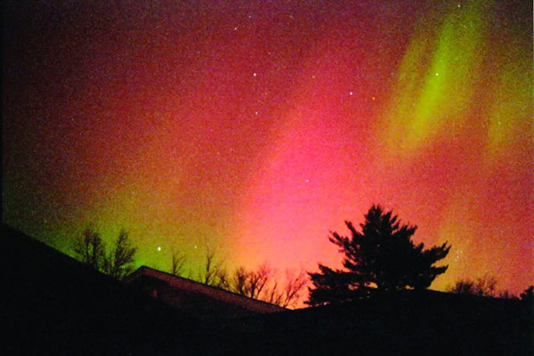
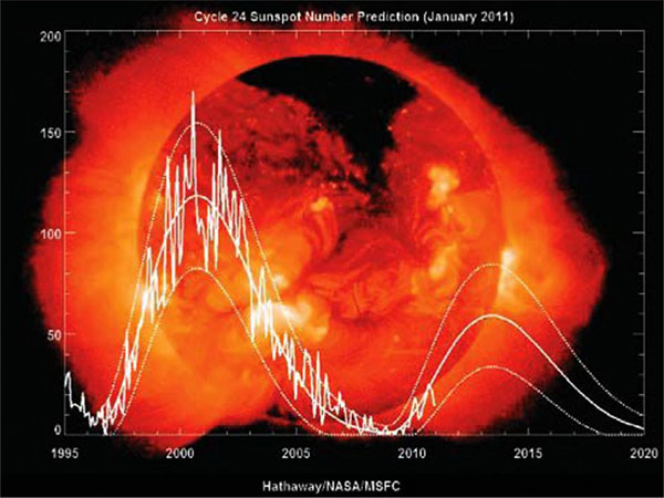
Although the sun can become disturbed at any time, solar activity is correlated with the approximately 11-year cycle of spots on the sun’s surface. We are just coming out of a minimum in the solar cycle and headed for the next maximum, predicted to occur around the middle of 2013. How significantly will GNSS users be affected? In this month’s column, two ionosphere experts tell us what might be in store.
INNOVATION INSIGHTS by Richard Langley
“HERE COMES THE SUN / here comes the sun / And I say / it’s all right.”
Is it? Of course, George Harrison was referring to the welcome return of the sun after a long dreary English winter. But can GNSS users sing the same refrain?
The signals from global navigation satellites must transit the ionosphere on their way to receivers on or near the Earth’s surface. The passage exacts a toll in the form of an added delay of the pseudorandom-noise-code signals and an advance of the phase of the signals’ carriers, due to the presence of the ionosphere’s free electrons. These perturbations must be ameliorated in some way to achieve high accuracy in GNSS positioning, navigation, and timing applications.
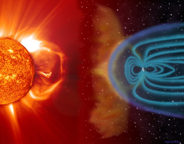
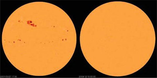
Where do the ionosphere’s electrons come from? For the most part, they are valence electrons, stripped from upper atmosphere atoms and molecules by the extreme ultraviolet light continuously emitted by the sun. On the Earth’s night-side, the electrons and the ionized atoms and molecules tend to recombine. This ionization and recombination process, along with the interactions of the particles with the Earth’s magnetic field, governs the density of the electrons at a particular location and time. The ionosphere is also affected by the solar wind, and its associated magnetic field, but the cocoon established by the Earth’s magnetic field (the magnetosphere) tends to deflect the solar wind so that it usually has little influence on the ionosphere.
Normally, the sun is quiescent: its electromagnetic and particle radiation is fairly constant, and its effects on the ionosphere benign. The delay in GNSS code observations and the advance in phase observations can be readily estimated and removed from the observations using a variety of models and methods. However, the sun can become disturbed, giving rise to occasional violent outbursts with large increases in electromagnetic and particle radiation. These outbursts can radically change the distribution of the electrons in the ionosphere, reducing the effectives of some amelioration methods. The electron density variability can become so rapid that a GNSS receiver can lose lock on satellite signals. And an increase in the sun’s radio emissions can become so large as to drown out GNSS signals on the sunlight side of the Earth.
Although the sun can become disturbed at any time, solar activity is correlated with the approximately 11-year cycle of spots on the sun’s surface. We are just coming out of a minimum in the solar cycle and headed for the next maximum, predicted to occur around the middle of 2013. How significantly will GNSS users be affected? In this month’s column, two ionosphere experts tell us what might be in store.
GNSS satellite signals are affected by the space environment and the Earth’s atmosphere as they travel from satellites at an altitude of about 20,000 kilometers above the surface of the Earth to receivers located at, or close to, the surface.
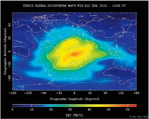
In the upper part of the Earth’s atmosphere, the ionosphere, which is located from about 80 to 1,000 kilometers above the surface of the Earth, satellite signals are affected by the free electrons stripped from atoms and molecules by ionization. The signals are refracted by this plasma, which changes their speed of travel. The effect is mainly a function of the number of free electrons present, the electron density.
In the lower parts of Earth’s atmosphere, in the troposphere and the stratosphere — where the atoms and molecules are electrically neutral — the satellite signals experience additional refraction. Here the effect is a function of pressure, temperature, and humidity. The effect of the troposphere and stratosphere is often just referred to as the “tropospheric effect” in GNSS positioning as it is in the troposphere where most of the neutral atmosphere refraction occurs.
The ionospheric and tropospheric effects on satellite signals must be accounted for in the GNSS positioning process in order to obtain reliable and accurate position solutions. In this article, we look at the ionospheric effect on satellite signals. Although the variation in signal speed is the largest direct ionospheric effect on the GNSS satellite signals, scintillation is another important effect. Scintillation occurs when irregularities in the electron density of the ionosphere cause rapid changes in the phase and amplitude of the transmitted signals. These changes might cause a GNSS receiver to lose lock on a satellite signal. This means in practice that satellite signals are lost, or signal tracking can be rather difficult, during scintillation events. However, we restrict our article to the subject of the propagation speed of the signals and do not consider scintillation further.
In the following, we review characteristics of the ionospheric effect on GNSS satellite signals as well as the predictions of increased ionospheric activity for the coming years and the consequences for GNSS users.
Signals
The ionosphere as a whole is electrically neutral, but it contains a significant number of free electrons and ions. The negatively charged free electrons affect the electromagnetic satellite signals in various ways. Most important is the signal delay affecting code (pseudorange) measurements, also called the “ionospheric delay” (and the associated advance of carrier-phase measurements), which is caused by a change in the refractive index along the signal path. The refractive index changes continuously as a function of the composition of the transmission media all the way from the satellites to the GNSS receivers.
For the majority of the signal path — that is, from the satellite at an altitude of about 20,000 kilometers down to approximately 1,000 kilometers above the surface of the Earth — the change in the refractive index is usually sufficiently small to ignore when the GNSS satellite signals are used for positioning at the surface of the Earth (although, at times, the region above the ionosphere — the plasmasphere — can affect GNSS signals). We therefore use the approximation that the first part of the signal path is in a vacuum where the propagation of GNSS satellite signals is not affected.
Then, when the signals enter the ionosphere, we must consider the signal delay, and even though the density of electrons is largest at an altitude around 300 kilometers, we must consider the total number of electrons experienced by a satellite signal all the way through the ionosphere.
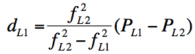
The size of the so-called first order effect of the signal delay, d, given in meters, can be modeled by the expression in Equation (1),
(1)
where f is the GNSS signal frequency, for instance 1.57542 x 10⁹ Hz for the GPS L1 frequency. The constant 40.3 is derived from the values of the electron charge, the electron mass, and the permittivity of free space. Finally, TEC is an abbreviation for total electron content and this value is given by integrating the number of free electrons along the signal path in a cross section of one square meter.
It turns out that the “delay” affecting carrier-phase measurements has exactly the same magnitude as the signal delay but is negative. In other words, the phase is advanced.
In practice, for single-frequency receivers, it is not possible to obtain the actual number of electrons along the signal path for every satellite signal, and we therefore need other models to predict or estimate the electron density or the signal delay.
A large number of models and methods for estimating the ionospheric signal delay have been developed. A comparison of some of them is given in a paper by Allain and Mitchell (see Further Reading). The most widely used model is probably the Klobuchar model, named after John Klobuchar, its developer. Coefficients for the Klobuchar model are determined by the GPS control segment and distributed with the GPS navigation message to GPS receivers where the coefficients are inserted into the model equation and used by receivers for estimation of the signal delay caused by the ionosphere.
Dispersion. The ionosphere is dispersive for radio waves, which means that the GNSS ionospheric signal delay is a function of the frequency of the signal. If pseudorange measurements from more than one frequency are available, for instance from dual-frequency GPS receivers, this can be used for enhanced modeling of the ionospheric effect by using combinations of the measurements made on both frequencies.
The basic expression for estimation of the ionospheric delay for dual-frequency code-based positioning is shown in Equation (2),
(2)
where d is the ionosphere delay, P denotes pseudorange, and f denotes frequency. The subscript notation L1 and L2 refers to the GPS L1 and L2 frequencies, respectively.
For high-accuracy carrier-phase-based positioning, an ionosphere-free combination of carrier-phase observations of the L1 and L2 frequencies is often used to reduce the effect of the ionospheric phase advance in the positioning process.
Estimating the ionosphere delay with Equation (2) for code observations or utilizing the ionosphere-free combination of the phase observations compensates for the first order ionospheric effect. This is the major part of the effect, but higher order effects are present, and the size of the residual higher order effects is increased (up to some centimeters) when the ionospheric activity is increasing.
For high-accuracy applications, the difference in the time of transmission and reception of the satellite signals of the various frequencies also must be considered as the signals on various frequencies are not transmitted from the satellites (nor received at a GNSS receiver) at exactly the same time epochs. These differences are normally referred to as the satellite and receiver differential code biases.
It is important also to note in this context that the noise level on the pseudorange corrected for the ionosphere and on the ionosphere-free carrier-phase observation is increased compared to using the pure single-frequency observations for positioning, but nevertheless these first-order approaches are used successfully in most software and receiver firmware for dual-frequency positioning.
Further developments of ionosphere-free combinations will evolve in the future as the new GPS L5 frequency and the new Galileo and GLONASS frequencies become fully available for multi-frequency ionosphere-free combinations. These more advanced combinations have the potential to further reduce the residual effect of the ionospheric delay in the positioning process.
Summing up, the GNSS signal delay caused by the ionosphere is a function of the electron density of the ionosphere. But what is driving the variation in electron density, and how do we know if it is changing?
Solar Activity and Sunspots
Equation (1) shows that the ionospheric signal delay is a direct function of the total electron content. The number of free electrons in the ionosphere is not constant; it varies significantly with time and space. The number of free electrons is driven by the ionization and recombination processes of the ionosphere, and these processes are in turn driven mainly by extreme ultraviolet radiation from the sun. Radiation from other cosmic sources also has an influence but it is minor compared to the effect of the solar radiation. There are also significant short-term (minutes to hours) changes caused by wave activity from the neutral atmosphere. The ionosphere itself is embedded in the neutral atmosphere — at these altitudes this is known as the thermosphere. The thermosphere is in constant movement due to waves and tides that are generated in situ or ascending from the underlying atmosphere. This thermosphere activity affects the ionosphere and causes some of the short-term variability in the electron density. However, the term “ionospheric activity” generally refers to the variability in electron density as driven by solar activity.
The fact that ionospheric activity is mainly driven by solar activity implies that the temporal variation of the electron content of the ionosphere follows a daily cycle, with the largest TEC values in the early afternoon local time, when the effect of the solar radiation has reached a maximum. Consequently, we see the lowest activity late at night just before sunrise.
There is also a geographic variability in the electron content with the highest electron density in the equatorial region and the lowest density in the high latitude regions. The latter, however, is affected by a larger variability, correlated with auroral activity.
The geographic variation of TEC is illustrated with a global ionosphere map from the Center for Orbit Determination in Europe (CODE) shown in Figure 1. Global ionosphere maps are generated at CODE on a daily basis, and the maps are available on the CODE website (see Further Reading).
Figure 1. Global ionosphere map for November 22, 2010, at 14:00 UTC. (Map generated by CODE, University of Bern.)
The TEC is provided in TEC units (TECU), where one TECU equals 1016 electrons per meter squared.
The sun also emits a constant flow of charged particles called the solar wind. The particles, mostly electrons and protons with energies between about 10 and 100 kilo-electron-volts, travel at an average speed of about 450 kilometers per second, but varying from 200 to 900 kilometers per second depending on solar activity. Although the Earth’s magnetosphere deflects most of the solar wind, the interplanetary magnetic field, which is associated with the solar wind, can cause disturbances in the geomagnetic field. When this happens, particles of the solar wind enter the geomagnetic field and cause increased ionization in the ionosphere. The solar wind therefore also has a large influence on the variability of ionospheric activity. Also, sudden eruptions of the sun such as solar flares and coronal mass ejections (CMEs) cause increased ionization and thereby a larger ionospheric variability.
Figure 2 shows a CME blast and subsequent impact at the Earth.
Figure 2. Coronal mass ejection (CME) and subsequent impact at the Earth. The left part of the illustration is composed of an image from NASA’s Solar Dynamics Observatory spacecraft superimposed on an image from the Solar and Heliospheric Observatory spacecraft jointly operated by NASA and the European Space Agency. The CME cloud arrives at the Earth about two to four days later and is shown being mostly deflected around the Earth’s magnetosphere. The blue paths emanating from the Earth’s poles represent some of its magnetic field lines. (Image: NASA/Goddard Space Flight Center.)
Solar activity and the quantity of emissions from the sun are highly correlated with the number of sunspots on its surface. A sunspot looks like a dark spot because the temperature in a sunspot is lower than that in its surroundings. The generation of sunspots is not well understood, but it is related to anomalies in the solar magnetic field. What is well known, however, is the history of the number of sunspots, because these have been observed since the early 1600s.
The number of sunspots generally follows a cycle of about 11 years. During the last few years (2007–2009), we have experienced a time period with a low number of sunspots. In fact, there were many days in a row without any sunspots visible (see Figure 3). During the next three to four years, the number of sunspots is expected to increase, and this will be followed by a decrease until we reach a new period of low solar activity in 2019–2020.
Figure 3. Images of the sun taken by the Solar and Heliospheric Observatory spacecraft. On the left is an image taken on March 27, 2001, at the peak of the last sunspot cycle. The daily sunspot count was 241. On the right is an image taken on December 15, 2008, near the minimum of the last sunspot cycle, showing no sunspots. (Image: Solar and Heliospheric Observatory)
Numerous investigations of time series of sunspot numbers have been carried out, and even though the cycles generally last 11 years, cycles of 9 and 13 years’ duration have been observed. Also, the cycles vary with respect to the maximum number of sunspots observed during a cycle, and various “cycles of cycles” appear to be present with respect to the strength of the sunspot cycles. For instance, a cycle with a period of about 420 years has been identified in the historic listings of sunspot numbers combined with other observations contributing to the knowledge of solar activity. A very low number of sunspots was observed for a number of years between 1645 and 1715 when the sun was especially calm. This period is often referred to as the Maunder Minimum after the solar astronomer Edward W. Maunder. If the theory of the 420-year cycle is correct, then we will see a period with lower solar activity and fewer sunspot numbers by the end of this century.
But let’s turn our attention to the previous and current sunspot cycles referred to as cycles number 23 and 24 (The 1755–1766 cycle is traditionally numbered “1.”). A new cycle begins with the first observed high-latitude, reversed-polarity sunspot. Reversed polarity means a sunspot with opposite magnetic polarity compared to sunspots from the previous solar cycle. Sunspots from the new and previous cycles initially coexist. Eventually, only the new-cycle sunspots are present. Cycle 24 began on January 4, 2008, when the first reversed-polarity sunspot appeared.
Analyses of observations of solar activity show that the density of the solar wind increases with increasing sunspot number. Also, with a large sunspot number, solar flares and CMEs happen more frequently. Ionospheric storm activity is more common when the sunspot number is high, and this activity increases the variability in ionospheric delays. This all adds up to an increased number of free electrons in the ionosphere and a larger variability, which provides a larger and more variable signal delay for all types of GNSS-based positioning, navigation, and timing during periods with high sunspot numbers.
We know that the sunspot number is expected to increase during the next three to four years. What can be expected and what can we do to minimize the effects of the increased ionospheric activity on positioning, navigation, and timing applications?
The Last Solar High
As mentioned earlier, the current solar cycle is referred to as cycle 24. During the last solar cycle, cycle 23, the GNSS community was alert and aware of what could happen, and therefore many events were observed and analyzed. Among the most well-known events is a sequence of storms during October and November 2003, commonly referred to as the Halloween Storms. The most extreme was the storm on October 30, 2003, which resulted from a CME on October 29 at 20:49 UTC, which subsequently impacted Earth’s magnetic field at 16:20 UTC on October 30 and produced a great geomagnetic storm, which lasted for many hours.
Effects on GPS positioning of this storm have been documented by the GNSS research group of the Royal Observatory of Belgium, where kinematic analyses of data from 36 GNSS stations in Europe showed position errors of more than 10 centimeters in the horizontal and up to 26 centimeters in the vertical between 21:00 and 22:00 UTC on October 30. The position errors were largest for locations in northern Europe including Sweden and Norway. The data analysis was carried out using high-quality carrier-phase data, and the processing was based on using an ionosphere-free linear combination of observations from the L1 and L2 frequencies, whereby the first-order effect of the ionosphere is removed from the results. The position errors are thus caused by mainly higher order ionospheric effects.
For navigation-grade GPS positioning, a U.S. National Atmospheric and Oceanic Administration technical memorandum (see Further Reading) reported that the Wide Area Augmentation System (WAAS) vertical error limit of 50 meters was exceeded for a period of about 11 hours on October 30, 2003. This means that, in practice, WAAS was not available for precision aircraft approaches during that time. The European Geostationary Navigation Overlay Service (EGNOS) was not transmitting during the storm, but simulations carried out later by ESA showed that the boundary regions of the EGNOS coverage area would have been especially affected by a reduction in service availability of about 20–60 percent during that day. The simulations also showed, however, that in the center of the EGNOS coverage area (in the vicinity of northern Italy), the effect would have been much smaller with a reduction in service availability of only 5–6 percent over the day.
Such large storms are also often accompanied by displays of aurora (aurora borealis and aurora australis) at lower latitudes than normal. Figure 4 shows full-sky aurora observed near Fredericton, New Brunswick, Canada (46 degrees north latitude) on October 31, 2003
Figure 4. Photo of red and green auroras observed near Fredericton, New Brunswick, Canada (46 degrees north latitude) early on October 31, 2003. (Courtesy of Richard and Marg Langley.)
During a storm event on November 20, 2003, auroral activity was visible at mid-latitudes over most of North America as far south as Florida and in southern Europe including Italy and Greece.
Eruptions of the sun, often occurring in connection with high sunspot numbers, can have other effects besides the influence on GNSS-based positioning, navigation, and timing. Power-grid blackouts are known to have happened because of geomagnetic storms in connection with the sunspot peaks of both cycles 22 and 23 in 1989 and in 2003, respectively. For instance, the southern part of Sweden experienced a power blackout for several hours during the evening of October 30, 2003.
Also, orbiting satellites can experience problems with the increased radiation and solar wind density. Solar panels are, for instance,
susceptible to increased aging. And many types of satellite communication can be affected by increased ionospheric activity, not only GNSS satellite signals. Signals used for satellite phones, satellite TV, and so on can be affected.
Another phenomenon that can affect GNSS positioning is solar radio storms (also referred to as solar radio bursts) caused by events on the sun, often a solar flare, which creates radio waves that are emitted from the solar atmosphere and can propagate to the Earth where they cause an increased noise level in radio signals. Solar radio storms can cover a wide range of frequencies, including the frequencies used for GNSS. One such storm occurring on December 6, 2006, did affect GNSS positioning. With an increased noise level on the satellite signals, GNSS performance is reduced. If the noise level becomes too large, as a consequence of, for instance, a solar radio storm, GNSS receivers will lose lock on the GNSS signals, whereby positioning performance is further reduced or positioning might even be impossible. Solar radio storms are expected to happen more frequently during the peak of a solar cycle, but the event in December 2006 happened during a period with low solar activity, highlighting the fact that GNSS performance can be affected at any time, even when the sunspot number is low.
Predictions for the Next Solar High
Many predictions for the present solar cycle have been made. Because of the very long period with low solar activity during 2007–2009, some predictions expected a sudden outburst of activity and a very large cycle maximum, while other predictions foretold another increase in solar activity might not occur for many years.
However, with a general increase in the number of sunspots during 2010, it looks like we are now well into solar cycle number 24. Things can still change, but the current predictions say the maximum of the current solar cycle will be lower than the maximum of the last cycle encountered in 2001.
Predictions of sunspot numbers are based on history, logged information on sunspot numbers, and on observations of related geomagnetic activity.
The latest prediction for the current cycle as generated by NASA is shown in Figure 5.
Figure 5. Sunspot cycle 23 and predictions for cycle 24 from NASA’s Marshall Space Flight Center. (Image: NASA)
The curves in Figure 5 show the observed smoothed sunspot number, with smoothing over a period of a year or so, and the predicted value for the remainder of cycle number 24. The dotted lines indicate the observed or expected range of the monthly-averaged sunspot numbers. The plot is updated every month as new data is obtained.
The current prediction for cycle 24 gives a smoothed sunspot number maximum of about 59 in June/July of 2013. This peak is much lower than that of the previous cycle. We are currently two years into cycle 24 and the predicted size continues to fall. According to forecasters, predicting the behavior of a sunspot cycle is fairly reliable once the cycle is well under way (about three years after the minimum in sunspot number occurs). Prior to that time, the predictions are less reliable but nonetheless equally as important.
Even though the maximum of the current solar cycle is expected to be lower than the last peak, it is important for GNSS users to be aware of the effects to be expected during the coming years.
Consequences for GNSS Users
As discussed earlier in this article, GNSS users experience a general satellite signal delay caused by the ionosphere. This signal delay is always present but varies in size. The delay is generally well modeled by most receivers and software to an extent that makes GNSS useable for all of the purposes we know today.
During enhanced ionospheric activity, GNSS users can experience residual ionospheric effects, which can cause reduced positioning, navigation, and timing performance. In such cases, dual-frequency receivers might improve the situation because of the enhanced possibilities for handling the ionospheric effect with dual-frequency data.
During enhanced ionospheric or geomagnetic storm activity caused by sudden eruptions of the sun, increased ionospheric variability will occur. Apart from causing an increased ionospheric signal delay, and thereby increased residual effects in the positioning process, this will also cause increased scintillation effects. These might cause GNSS receivers to lose lock on some or all GNSS satellite signals, reducing performance of the GNSS receiver. In the few very worst cases, GNSS-based positioning, navigation, and timing might not be possible at all for a short interval of time during very high ionospheric activity.
These worst-case scenarios are more prone to happen close to the peak of a solar cycle, which we will meet next during 2013–2014.
However, it is worth noting that for the next peak of the solar cycle, we are much better prepared for the consequences than during the last cycle. GNSS software and receiver technology has been improved to better resist the challenges of increased ionospheric activity during this solar cycle. The improvements are based on experiences gained during the last solar cycles and are to the benefit of many GNSS users. For example, users of wide area augmentation systems such as WAAS and EGNOS have correction and integrity information available, which can be a great help in identifying time epochs when positioning and navigation solutions might not be trustable because of increased ionospheric activity. The integrity information is transmitted from geostationary satellites, and during time periods with extremely high ionospheric activity, the signals with integrity information might be disrupted. This should, however, be detected by the GNSS receiver, so warning messages will be displayed for navigators.
High-accuracy real-time kinematic (RTK) positioning is today often carried out with RTK correction data from a service provider generated using a network of reference stations. Here, indications of increased ionospheric activity can be detected by the software operated by the service provider, and warnings can be distributed to the RTK users.
Warning systems have been improved, and a number of sites on the Internet provide information on current and predicted ionospheric activity (see Further Reading).
Also, in the future, GNSS users will be able to benefit from the increased number of GNSS frequencies available. These frequencies open up opportunities for new and improved methods for correction of the ionospheric delay to the benefit of users who will experience more stable and reliable GNSS performance.
Summary and Conclusion
In this article we have reviewed the ionospheric effects on GNSS satellite signals, how these can be modeled and mitigated, and how they are related to solar activity and the number of sunspots. We have also described how sudden eruptions of the sun can cause increased ionospheric activity and how these events are often correlated with a high sunspot number. Some examples of consequences for GNSS users during the last solar high have been provided, and we have evaluated the predictions for the next solar high and possible consequences for GNSS users.
We are heading towards a period of increased solar activity. GNSS users must expect more disturbances compared to what we have seen for the last four to five years. The peak of the current solar cycle is expected to be lower than the last peak, and therefore consequences for GNSS users should also be less significant. Most of the time GNSS will work very well. But we will likely see a few days with major effects, and since the number of GNSS users is increasing, the overall consequences might also be more severe, not because the ionospheric activity is worse, but simply because more people will be affected.
ANNA B.O. JENSEN is the owner of AJ Geomatics in Copenhagen and a part-time associate professor of the National Space Institute at the Technical University of Denmark (DTU Space). She has a Ph.D. from the University of Copenhagen with co-supervision from the University of Calgary, and has worked in research and development within GNSS and geodesy for more than 15 years. Her current research interests include ionospheric modeling, high accuracy positioning, and navigation in the Arctic.
CATHRYN MITCHELL is a professor in the Department of Electronic and Electrical Engineering at the University of Bath in the United Kingdom and heads the INVERT Centre, which studies inverse problems and tomography over a range of scientific fields, including navigation, space science, and medical imaging. She has a Ph.D. from the University of Wales in Aberystwyth. Mitchell has a particular interest in the use of GNSS measurements to characterize and map the ionosphere.
FURTHER READING
• Introduction to the Ionosphere and Its Effects on GNSS
“The Perfect Solar Storm” by D.N. Baker and J.L. Green in Sky & Telescope, Vol. 121, No. 2, February 2011, pp. 28–34.
Severe Space Weather Events–Understanding Societal and Economic Impacts: A Workshop Report by the National Research Council Committee on the Societal and Economic Impacts of Severe Space Weather Events, published by National Academies Press, Washington, D.C., 2008; available on line: http://www.nap.edu/openbook.php?record_id=12507.
“Combating the Perfect Storm: Improving Marine Differential GPS Accuracy with a Wide-Area Network” by S. Skone, R. Yousuf, and A. Coster in GPS World, Vol. 15, No. 10, October 2004, pp. 31–38.
“Space Weather: Monitoring the Ionosphere with GPS” by A. Coster, J. Foster, and P. Erickson in GPS World, Vol. 14, No. 5, May 2003, pp. 42–49.
The High-Latitude Ionosphere and its Effects on Radio Propagation by R.D. Hunsucker and J.K. Hargreaves, published by Cambridge University Press, Cambridge, U.K., 2002.
“GPS, the Ionosphere, and the Solar Maximum” by R.B. Langley in GPS World, Vol. 11, No. 7, July 2000, pp. 44–49.
• The Effects of the Halloween Storms on GNSS
“Impact of the Halloween 2003 Ionospheric Storm on Kinematic GPS Positioning in Europe” by N. Bergeot, C. Bruyninx, P. Defraigne, S. Pireaux, J. Legrand, E. Pottiaux, and Q. Baire in GPS Solutions, Online First, 2010, doi: 10.1007/s10291-010-0181-9.
“Assessment of EGNOS Performance Under Worst-Case Ionospheric Conditions (Solar Storm of October/November 2003)” by C. Montefusco, J. Ventura-Traveset, B. Arbesser-Rastburg, F. Froment, D. Flament, E. Tapias, S. Radicella, and R. Leitinger in EGNOS – The European Geostationary Navigation Overlay System – A Cornerstone of Galileo, ESA SP-1303, published by the European Space Agency Publications Division, Noorwijk, The Netherlands, 2006, pp. 259–268.
Halloween Space Weather Storms of 2003 by M. Weaver, W. Murtagh, C. Balch, D. Biesecker, L. Combs, M. Crown, K. Doggett, J. Kunches, H. Singer, and D. Zezula, NOAA Technical Memorandum OAR SEC-88, published by the Space Environment Center, National Oceanic and Atmospheric Administration, Office of Oceanic and Atmospheric Research, Boulder, Colorado, June 2004; available on line: http://www.swpc.noaa.gov/Services/HalloweenStorms_assessment.pdf
• Ionospheric Models and Corrections
“Ionospheric Delay Corrections for Single-Frequency GPS Receivers over Europe Using Tomographic Mapping” by D.J. Allain and C.N. Mitchell in GPS Solutions, Vol. 13, No. 2, 2009, pp. 141–151, doi: 10.1007/s10291-008-0107-y.
“Ionospheric Time-Delay Algorithm for Single-Frequency GPS Users” by J.A. Klobuchar in IEEE Transactions on Aerospace and Electronic Systems, Vol. AES-23, No. 3, May 1987, pp. 325–331, doi: 10.1109/TAES.1987.310829.
“Global Ionosphere Maps Produced by CODE” on the website of the Astronomical Institute of the University of Bern, Bern, Switzerland: http://aiuws.unibe.ch/ionosphere/.
• Solar Cycle and Solar Weather Predictions:
“Solar Weather Event Modelling and Prediction” by M. Messerotti, F. Zuccarello, S.L. Guglielmino, V. Bothmer, J. Lilensten, G. Noci, M. Storini, and H. Lundstedt in Space Science Reviews, Vol. 147, 2009, pp. 121–185, doi: 10.1007/s11214-009-9574-x.
“Predicting Solar Cycle 24 and Beyond” by M.A. Clilverd, E. Clarke, T. Ulich, H. Rishbeth, and M.J. Jarvis in Space Weather, Vol. 4, S09005, 2006, doi: 10.1029/2005SW000207.
I was fortunate enough in 1993 to have three minutes of fame on 60 Minutes in a program about GPS that aired between Christmas and New Year’s that year. Also in the 13-minute segment was a short demo of a GPS PLGR. A reporter asked a lieutentant colonel outside Shreiver AFB to demonstrate how far and in what direction New York City lay. The colonel said, given the bearing and distance shown on the two-line display, he theoretically could navigate all the way from Colorado to New York. That lieutenant colonel was Willie Shelton. So I have hope that he will do the right thing for GPS during his tenure as head of Space Command. [System news, p. 14]
— Len Jacobson Global Systems and Marketing Inc. Long Beach, California
Down and Deep
Wow! The article “Down and Deep” by Frank van Diggelen [December 2010 issue] was so useful for explaining the alternatives to GPS to a bunch of suits that normally don’t get it. I’ve shared it with many of my colleagues and they’ve all had the same reaction. Thank you!
— Ed Harrison Orange County Probation Department Santa Ana, California
Can the development and use of smart technologies actually render us dumber? Have we already lost a mental step or two, as we equip ourselves fearlessly for the future?
Marshall McLuhan, the “medium is the message” guy from back when, preached that tools numb whatever part of the body they amplify. By extrapolation, location-enabling tools render us less aware of our actual place.
It causes me some discomfort to float this topic in the standard bearer for an extremely advanced high-tech industry. Yet I also felt acute and nearly continuous discomfort while reading a book over the winter holidays; a poke here, a prick there, until I was sitting on pins and needles. I had selected the volume with an eye to finding out why my adult and near-adult children, actively engaged online, have little patience with the printed page anymore, and find books practically abhorrent.
Of course, every generation has its preferences, but this trend troubles me because it seems associated with a reluctance to truly explore, to think critically, at length, and in some depth. Also, it’s not limited to twentysomethings. I find plenty of affected folks at every age.
The book is The Shallows: What the Internet Is Doing to Our Brains, by Nicholas Carr. It provided grist galore in the online/print dichotomy — the changes in how we look for, absorb, process, and store information. And as said, it generated no little discomfort as I realized how much I, too, have changed in a decade and a half of increasing online activity, at work and in leisure.
I began to wonder, as I read, where that other game-changing modern technology, global satellite navigation, enters the picture. Sure enough, it surfaced on page 212.
A neuroscientist engaged in studying the brains of London taxi drivers found that their hippocampal area increased in gray matter volume because of the huge amount of street names and traffic-flow data they must memorize. She worries that when cabbies use GPS, that knowledge base will shrink, and possibly that area of the brain will atrophy or fail to develop.
This is perhaps a trivial example that has little to do with you and me. But consider your experience and your awareness as you follow, head down, your PND or a cell-phone screen to your next destination. Do you register the environment en route, possibly including hazard factors? Do you notice other points of interest that might enrich your experience, occasion a stop, detour, or return trip — or even constitute a better destination? Once arrived, could you find your own way there again, or have you become dependent on silicon and signals?
GNSS brings undeniable benefits in areas where it creates capabilities that did not exist before, such as measuring millimetric sway of tall buildings or changes in sea level; that is, largely in professional areas. But where it offers convenience or shortcuts in everyday life, that can be a more double-edged sword. The Internet has proved so; recall also canned, frozen, and processed pre-prepared foods, once embraced as modern timesavers. We now find they stripped essential nutrients out of our diet, undermining health and helping create an obesity epidemic.
Spectracom, a global provider of time and frequency test and measurement solutions, will make available its new 16-channel GPS constellation simulator, the Pendulum GSG-55, in March. The GSG-55 is the latest in the Pendulum line of GPS receiver test instruments and part of its solution set for receiving, distributing, and validating GNSS systems.
With the enhanced signal generating capability of the GSG-55, it is possible to simulate Satellite-Based Augmentation Systems (SBAS), the company said. Navigation systems that use SBAS can improve the accuracy and reliability provided by the GPS satellite signals alone, enabling critical applications such as aircraft navigation, and surveying and mapping. SBAS simulation (support for Europe’s EGNOS and North America’s WAAS) is a new feature in the GSG-55. It is also able to generate white noise, making it possible to test receiver sensitivity under different signal-to-noise ratios.
“Many high-end GPS applications utilize 12-channel GPS receivers. Our new GSG-55 GPS constellation simulator can fully test those receivers with additional signals for more comprehensive testing in both development and production environments,” says Staffan Johansson, product manager at Spectracom.
The GSG-55 builds on the popular Pendulum GSG-54 eight-channel simulator including accurate testing of GPS timing receivers and portability through its compact and lightweight bench-top chassis. The GSG-55 also continues the Pendulum brand hallmark of ease-of-use. As such, the entire GSG family of GPS simulators has been improved based on customer feedbac, the company said.


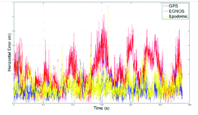


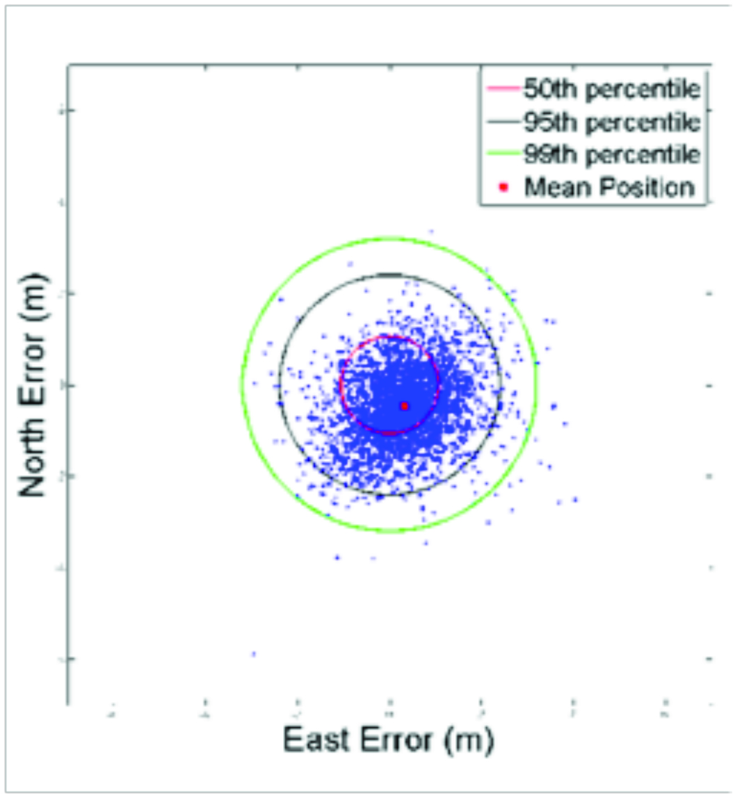

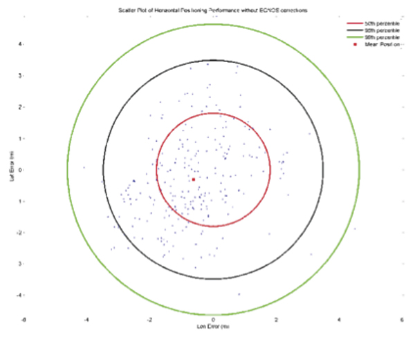
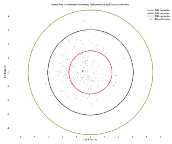

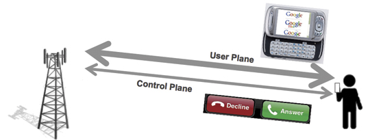


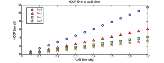


 Shelton Space Commander
 Des Dorides for European GNSS Supervisory Agency