Blog

  • A Look at the Rugged Handheld Algiz 7

    The warfighters have spoken. My correspondence lately has been full of questions about tablet and handheld computers. My sources at AT&T and Verizon tell me that the number of iPads in Iraq and Afghanistan have doubled in the last year alone. The problem is that Apple iPads and iPhones, for all their ubiquity, are not rugged in any sense of the word. Enter Handheld US with the Algiz 7.

    Algiz-7-on-snowy-ground-W

    The warfighters have spoken. My correspondence lately has been full of questions about tablet and handheld computers. Out of every 10 letters or emails, seven contain comments or questions about tablet type or handheld computers.

    Ever since the Apple iPad came bursting onto the portable computer scene, everyone else has been trying to produce a competitor. Now that the iPad 2 has bowed, everyone is once again behind the eight ball and struggling to catch up.

    My sources at AT&T and Verizon tell me that the number of iPads in Iraq and Afghanistan have doubled in the last year alone. Skype calls are the most frequent way our warfighters stay in touch with their loved ones. Viewing those you care about on a high-definition 10-inch color screen beats a MARS call any day!

    The problem, of course, is that Apple iPads and iPhones for all their ubiquity are not rugged in any sense of the word. You can make them more rugged with the excellent line of Otterbox cases I have reviewed in the past, but the fact remains that the iPad and iPhone are still not built from the ground up to be a rugged computing device, no matter how badly we think we treat them in our day-to-day work and commuting environment.

    The Swedes at the Gates

    Enter Handheld US, an affiliate of Handheld Group AB, a Swedish firm located in Lidkoping, which is a thriving metropolis of about 30,000 hardy inhabitants. Not surprisingly Handheld Group AB and Handheld US specialize in rugged handheld computers, like the Algiz 7, that are designed and built from the ground up for the rugged outdoors, for first responders, and for the military war zone environment.

    ROE – Rules of Engagement

    As many of my regular readers know, I review rugged military-compatible handheld computers on a regular basis. As with all the rugged computers I review, I put them through a series of torture tests. The ones that fail you never hear about, because I have a policy of never writing a bad review. Why should I waste my time and yours? After all, we both want to know about products that work as advertised, right? I know I do and be assured, BLUF, bottom line up front, the Algiz 7 lives up to its reputation as a rugged handheld or tablet computer that from all reports functions well in rugged military theaters such as Iraq and Afghanistan.

    Warfighters

    Several of our warfighters are currently using the Algiz 7 as well as many of the other Handheld US derivatives, many of them from companies such as Trimble that are repackaged and resold by Handheld US. To date it has been my experience that as a first responder or warfighter you cannot go wrong with any of the rugged Handheld US computers I have had the pleasure to review.

    Torture Tests

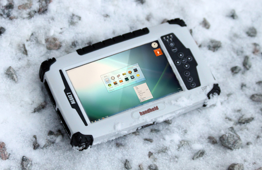
    As far as my torture tests are concerned, they usually involve lots of water, snow banks, and freezing temperatures, with some mud and ice thrown in for good measure, along with a few drops from several feet onto hard frozen ground. When I looked up Handheld Group AB and found their location in Sweden, it immediately became clear that the Handheld Group AB folks can test their computers the way I do almost any day of the week for a large portion of the year, just by stepping out their front door. Even so, I assiduously ran the Algiz 7 through all the torture tests and it survived admirably. Plus unlike many of the nearly sea-level tests in Sweden, my tests are performed at about 7,000 feet above sea level or higher, more closely resembling the altitudes in parts of Afghanistan.

    Specifications

    The word Algiz can mean many things, but is usually translated as “elk,” and that is a rugged animal. I see them occasionally in my backyard and they certainly survive in some rugged environments in the Rocky Mountains, so the name is fitting. The Algiz 7 certainly sounds better than the Elk 7.

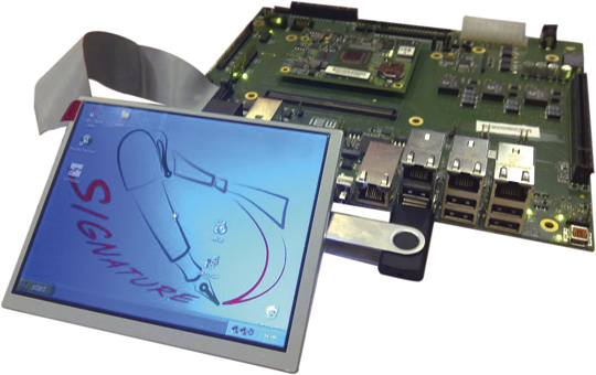
    The Algiz 7 is a rugged handheld Windows 7 computer with integrated GPS capability perfect for today’s warfighters in many respects.

    We have been batting the word “rugged” around for some time, and now might be a good time to define exactly what rugged means. I have told you about my unofficial tests that are based on some of the MilSpec (military specifications) standards and their readily available definitions. However, it is interesting to see how Handheld defines rugged. Handheld defines rugged in its literature as pertaining to environmental specifications, of which the three most common and useful are:

    • Temperature range,
    • MIL-STD-810F/G
    • IP

    Fortunately for users, these specifications are almost always prominently listed on the product data sheet, but what the heck do they really mean? How do they translate into real-world requirements, especially in battlefield conditions?

    The temperature specification defines the operational temperature range of the unit. Working with a unit above or below this specification may well cause the unit to fail when you need it most.

    I have defined MIL-STD-810F/G several times in the past, but for all the first-timers, it is a standard issued by the United States Army’s Developmental Test Command. The standard consists of a series of various environmental tests to prove that equipment qualified to the standard will survive in the field. The MIL-STDs (military standards) were originally designed specifically to test military equipment, but are now used to test a wide range of both military and civilian products, including mobile computers with GPS capabilities.

    Certainly the letters IP stand for many things in our high-tech world today, but here it stands for Ingress Protection, and an IP rating is used to specify the level of environmental protection of electrical equipment against solids and liquids. In other words, it tells us what amount of a certain size of solids or liquids can get inside the Algiz 7 enclosure and possibly damage the device. For those of you who must know, it is defined by international standard IEC 60529.

    The MIL-STD Testing Methods

    If you look it up, you will find that MIL-STD-810F/G comprises about 24 laboratory test methods that cover a wide range of environments, from the ability to perform at high altitude (method 500.4 and one I know well) to the ability to survive ballistic shock (method 522). No mobile computer has ever, to my knowledge, been tested to all 24 methods; many of the tests just do not apply to mobile computing, but generally speaking, the more methods tested (and passed), the more rugged the unit.

    The most rugged handheld GPS/computer devices (like the Handheld Nautiz X7, which I reviewed in GPS World in April 2010) have been tested on average to between 8 and 10 MIL-STD-810F methods. So when you are evaluating a data or specification sheet, pay close attention to the testing methods that apply to your specific situation. If you are a warfighter in Afghanistan and will be routinely working near or over 10,000 feet of elevation, make sure the unit has been tested to the MIL-STD method that covers that altitude.
    If you are going to be working in rapidly changing temperatures, make sure the unit has been tested for temperature extremes and temperature shock. Several of the units I have tested and you have not read about, in one of my columns at least, failed both the temperature and thermal shock tests.

    The IP Definitions: What Level Do You Need?

    IP ratings are routinely displayed as a two-digit number. The first digit reflects the level of protection against dust (think Afghanistan and Iraq). The second digit reflects the level of protection against liquids, most frequently water or snow (think the mountains of Afghanistan).

    Technically speaking, the dust specification has seven different levels, level 0 to level 6, and the water specification has nine different levels, level 0 to level 8. But practically speaking, rugged computers all must have at least a dust protection level of 5 and water protection level of at least 4 or they are simply not rugged in my book. Beware, because there are some computers that list themselves as being rugged that do not meet these minimum IP specifications. I, for one, would be wary of them in adverse environments. Be warned: At the operational ends of the scale, the IP levels can make a huge difference in a device’s ability to operate in severe environments and to a device’s overall longevity. For example, a dust level of 5 means that some dust may get into the device, whereas a level 6 device is completely sealed and dust proof.

    For example, an IP65-rated device, such as the Algiz 7, is totally dust proof and is capable of surviving rain showers and dust storms, but not total immersion in water. This device would be an excellent choice in either a very dusty or dirty environment or one where it may be possible to drop the unit in the occasional snow bank. Currently both AORs (areas of responsibility) for our warfighters come to mind. For more complete IP definitions see the Handheld-provided list below:

    Ingress Protection
    First digit = protection against dust:
    0: No protection
    1: Protection against solids up to 50 mm
    2: Protection against solids up to 12 mm
    3: Protection against solids up to 2.5 mm
    4: Protection against solids up to 1 mm
    5: Protection against dust; limited ingress
    6: Totally protected against dust

    Second digit = protection against water:
    0: No protection
    1: Protected against dripping water
    2: Protected against dripping water (tilted)
    3: Protected against water spray
    4: Protected against splashing water
    5: Protected against water jets
    6: Protected against a nozzle under pressure
    7: Protected against immersion (1 meter for 30 min)
    8: Protected against submersion (at depth, under pressure)

    Rugged Computers for Tough Environments

    If you are aware of your requirements, then knowing what the specifications of a particular device are and what they mean can provide invaluable information about how a unit will function in the field and over the long term. So, use the specifications to help you pick out the best unit for your situation. The bottom line for most warfighters is that a rugged computer, even though it may cost a little more up front, is guaranteed to be the most cost effective in the long run and will most probably be there when you need it, such as when your life depends on it. We know that is especially true of rugged computers with built-in GPS capabilities such as the Algiz 7.

    I hope, like me, you found the Handheld MIL-STD definitions and explanations helpful, but the question is how does the Algiz 7 really measure up? Handheld defines the Algiz 7 as super-rugged and ultra-mobile, but is that just hyperbole and marketing? Certainly the reports from warfighters that are currently using the Algiz 7 on the battlefield seem to defend the Handled description, but let’s check the specifications.

    The Algiz 7 sports a seven inch high definition (1024×600) resolution sunlight visible TFT LCD (thin film transistor liquid crystal display) touch color screen in a body that is 5.56″ (144 mm) x 9.5″ (242 mm) x 1.57″ (40 mm) and it weighs in at 2.42 lb (1.1 kg). But how does it measure up to those MIL-STD specifications we mentioned as being the definition of rugged?

    Operating: -9.4 °F to 140 °F (-23 °C to 60 °C), MIL-STD-810G
    Storage: -40 °F to 158 °F (-40 °C to 70 °C) MIL-STD-810G
    Drop: MIL-STD-810G 4ft Drop, Free to Concrete; 26 drops from 4 ft (1.22 m) MIL-STD-810G
    Vibration: MIL-STD-810G
    Sand & dust: IP65, MIL-STD-810G
    Water: IP65, MIL-STD-810G
    Humidity: MIL-STD-810G, 90% RH temp cycle 0 °C/70 °C
    Altitude: 15.000 ft (4572 m) at 73 °F (5 °C)

    As I said, I tend to be tough on equipment that I test, but even I did not drop it 26 times onto a concrete hard surface from a height of four feet. While I have been known to take a unit to the top of Pikes Peak, at a mere 14,100 feet, the temperatures rarely gets to 73 degrees Fahrenheit on top. In fact it is more like 7-10 degrees, and so I may have exceeded the MIL-STD specifications of the unit but with no noticeable affects.

    Visibility

    I can certainly vouch that the screen is viewable from almost all angles, and it is viewable in bright sun and reflected snow light. It is also viewable while wearing polarized sunglasses, which is a specification you may not see listed, but is critically important in snow country and one for which I always test. In many situations, polarized lenses do funny things to specially treated computer screens. I have seen computer screens that were just not visible or totally disappeared when viewed through polarized lenses. However, the Algiz 7 screen was easily visible, and if you are wearing heavy winter or work gloves, the attached stylus works well. Without gloves your finger is still generally the best stylus, but the screen on the Algiz 7 is capable of clearly portraying very tiny linkable objects, and at those times a stylus is more accurate than even our God-given digits.

    More Specifications

    The rest of the specifications for the Algiz 7 are as follows:

    Processor/memory: Intel Ultra Low Power Atom Z530 1.6 GHz processor (w/ US15W Chipset), 2 GB DDR2 RAM

    Data Storage/Disk: 64 GB SSD solid state hard drive

    Operating system: Microsoft Windows 7 Ultimate

    Screen: 7″ widescreen 1024×600 resolution TFT LCD MaxView sunlight readable resistive touchscreen display

    Keyboard/Keypad:

    10 keys:

    • Power key

    • Menu key (Controls Brightness, Volume, Battery Status, WiFi& BT On/Off, and 3G On/Off)

    • 4+1 Navigation/directional keys (Left, Right, Up, Down, Center for Enter)

    • 3x user programmable hotkey buttons that control up to 6 functions

    • On-screen QWERTY soft keyboard

    Battery: Hot-swappable Dual Li-Polymer Battery Pack, 2600 mAh each, support minimum 6 hours operation

    Connections:

    2 x USB 2.0 port (one fully waterproof, even when the latch is open)
    1 x 9-pin serial RS-232 port (fully waterproof, even when the latch is open)
    1x LAN
    1 x DC power port
    Input: 120-240 VAC, 50-60 Hz, 12 VDC Output
    Docking Connector (Contact Pin Type)
    1 x 4 pin docking
    Audio Out
    1 x Microphone
    Audio Integrated (one speaker)
    Fully Gobi™ 2000 PCIe module-ready

    Communication:

    Wireless LAN 802.11 b/g/n
    PAN: Integrated Bluetooth v.2.0 + EDR Compliant
    Integrated GPS Mediatek, WAAS/EGNOS capable
    WWAN (Optional) Gobi 2000 ready, supporting the following RF bands:
    • HSDPA/UMTS 800/850/900/1900/2100 MHz
    • Quad-band EDGE/GPRS/GSM – 850/900/1800/1900 MHz
    • Dual-band EV-DO/CDMA – 800/1900 MHz

    Camera: 2 Megapixel Camera + LED light

    Using the Algiz 7

    I will have to admit that the first time I saw the Algiz 7, I did not think it looked like a very rugged computing device, when in fact it may be one of the most rugged devices I have ever tested. Do not let appearances fool you; this is one very rugged mobile computing device.

    Light, Camera, Action

    For the warfighter and the first responders, the 2-megapixel forward-facing color camera and the LED light work extremely well. The LED light is very bright and not something you want to have flash or activate if you are working in a clandestine or stealth environment. But when you need it, it is extremely bright and works well. In an emergency it also works well as a flashlight.

    Skype and Batteries

    I ran Skype on the device with no problems. I once did a single battery hot swap and in the process did not drop the Skype call. I must admit I was impressed. As for battery life, the claimed six hours is a legitimate claim. I saw some days with five-plus hours under intensive work, and some days with seven-plus hours under a lighter load, so the six-hour battery life is the real deal. The dual Lithium Polymer batteries are very light and easy to swap out. For extended operations you will want a couple of spare batteries, and since they are hot swappable you will not lose one byte of data. For those of you with lots of sensors and accessories or the need for an even longer battery life, there is an extended life battery that provides 10-12 hours of service.

    Ports

    The ports on the Algiz 7 are extensive and all worked well for me. If there is a minor , I would say it is the number of USB 2.0 ports, as there was a time when I had a printer, full-sized keyboard, and some optional sensors connected and was looking for more USB ports. I simply used a USB port multiplier and that worked well, but this is obviously not ideal, especially if your USB devices draw power from the USB port. For most users this may never be a problem, but when you are testing a unit you like to push it to the limit.

    Communications

    The communications options are also quite extensive. As I said, I used Skype because that is what I had readily available. However, you can use 3G data and communications plans from several carriers as well. And since Verizon and AT&T both have extensive data networks in Iraq and Afghanistan, and there are tons of Wi-Fi sites, communications should never be a problem with the Algiz 7. You can take good-quality photos with the onboard 2-megapixel camera and quickly transfer them using 3G or Wi-Fi communications. Note: As I write this, certification of the Algiz 7 with the Verizon 3G network is still in the works but should be completed any day now.

    GPS

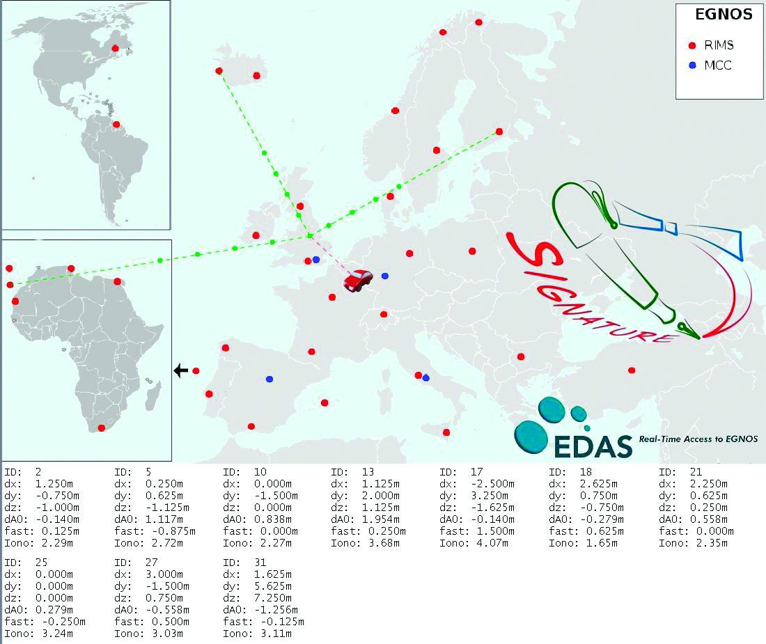
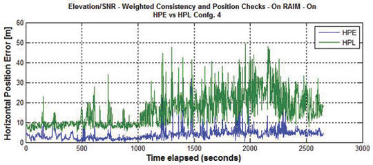
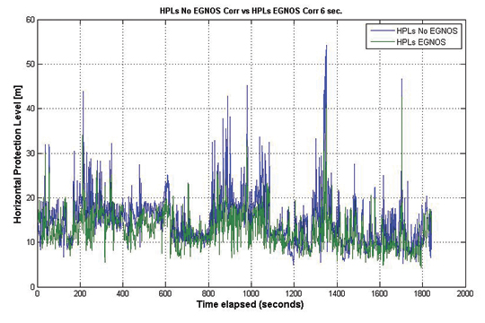
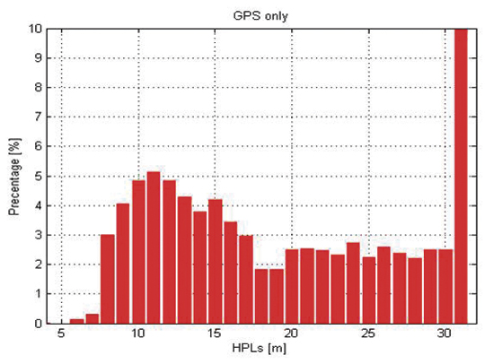
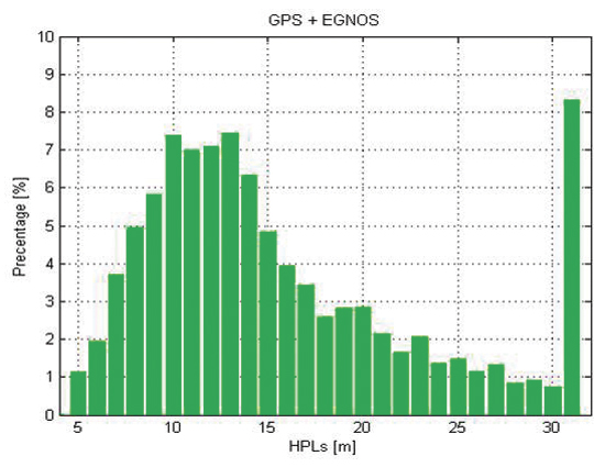
    The Algiz 7 has an integrated MediaTek GPS chipset, which is the same chipset that Garmin uses in many of its products. The Algiz 7 GPS is WAAS (Wide Area Augmentation System) and EGNOS (European Geostationary Navigation Overlay Service) capable. Adding the WAAS/EGNOS capability does make a considerable difference where availability, accuracy, and integrity issues are concerned. To most WAAS-enabled GPS devices, the GEO WAAS (Geosynchronous Orbit) signal due to geometry can be the apparent geometric equivalent of three additional GPS satellites in MEO (Medium Earth Orbit). WAAS of course is only available in the geographical area in and around the United States and EGNOS is only available in the European theater.

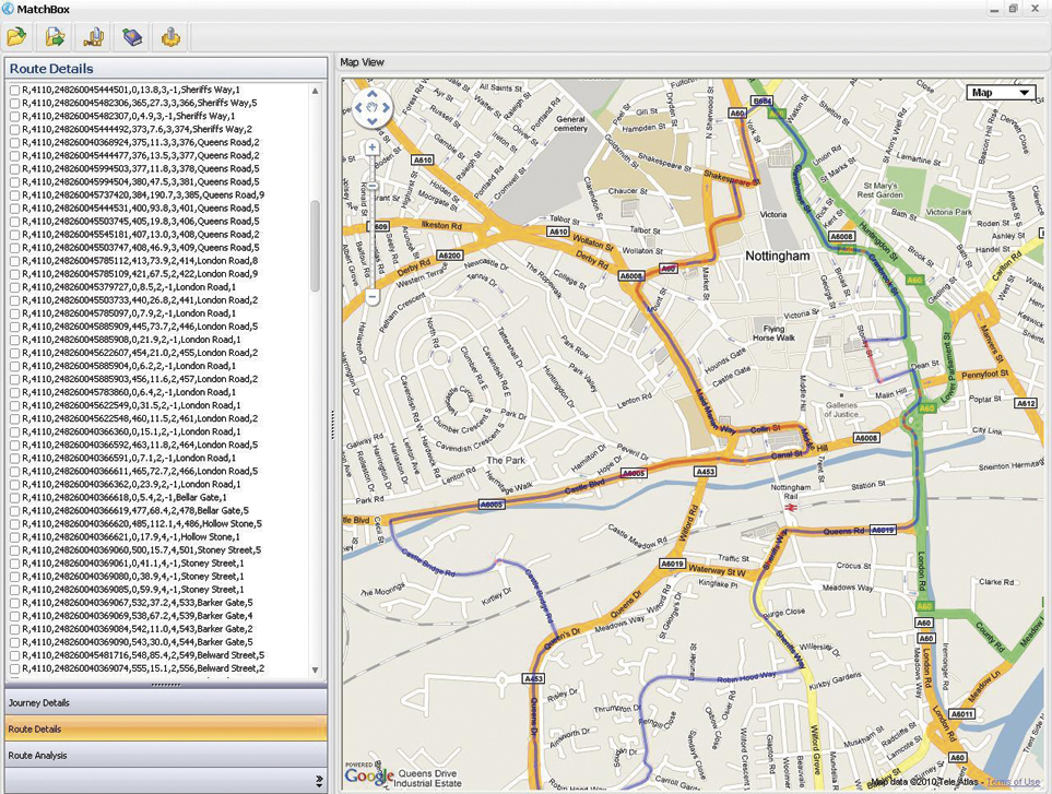
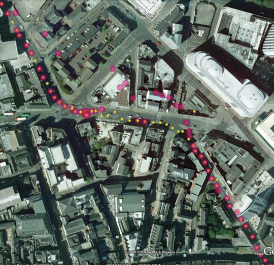
    I ran numerous navigation applications, and all the programs I tested found and integrated with the MediaTek GPS chipset output without problems. I tried several different maps and coordinate systems on the Algiz 7 without any significant issues. Not all coordinate and grid systems come as standard fare on the Algiz 7 but they can be found, downloaded, and used without issue.

    All in all, I was very impressed with the Algiz 7 as a handheld GPS capable device. Our warfighters should have no problems downloading and utilizing military maps and grid systems on the device. Google maps worked extremely well.

    Versatility

    While testing the Algiz 7 in the field, I once washed my muddy fingerprints off the screen with a handful of snow and then wiped it with a towel. I never feared I would cause any damage or lose any data because the 10 buttons on the face of the device are all covered and yet are clearly marked and readable. It is difficult to push a button by mistake. It never happened in the several weeks I was testing the device, and that is a big plus for our warfighters, who must frequently put the unit aside and come back to it later, say after a small engagement with the enemy.

    So the bottom line is that I am impressed with the Algiz 7, as I am with all the Handheld US products I have tested. I hope more warfighters and military procurement offices give it a shot. They won’t be disappointed.

    Until next time, happy navigating.

  • Beyond Hyper-Local and Location Enhanced

    Be all you can be. Being location enabled or “hyper local” isn’t enough. Mobile applications are also trying to increase discoverability, push into Group-On couponing territory, and proactively deliver more relevant recommendations to users. Loopt announced limited-time and perishable inventory deals to users within proximity. Google has introduced an “open now” filter to local mobile search to find nearby businesses that are open. Not content to focused on their core check-in business (“I am the proud mayor of Barney’s Beanery”), foursquare is now recommending places near you, based on previous check-in activities, user profiles, and what your friends like. On the foursquare blog, Dennis Crowley suggests “You’ll be surprised by what you get when searching for really specific things, like ‘’80s music,’ ‘fireplaces,’ ‘pancakes,’ ‘bratwurst,’ and ‘romantic’.” Evenings with Crowley must be, well, surprising. Very.

    Mass geo shopping. It is large-scale and geo-specific and, most interestingly, it comes from a carrier. AT&T and Placecast together launched ShopAlerts. AT&T subscribers can opt in and receive offers, rewards, and coupons based on each individual’s geolocation. AT&T will create geofences (virtual geographic perimeters) around retailers, events, or geographic areas to optimize relevancy. This isn’t so different than what some of the location-enabled social network applications (Booyah!, foursquare, Loopt) are doing, but it is significant because of the scale and reach that a carrier brings.

    Making money? Ever since Google offered free mobile navigation and others app providers followed suit, content providers have struggled to find ways to monetize their applications. Many have looked to mobile advertising for revenue. But mobile advertising hasn’t developed quite as fast as many predicted, although it is still a growing and big market. Apple’s iAD mobile advertising efforts have been a disappointment. Industry insiders say iAD fill rates have fallen to less than 10 percent and Apple has halved its minimum advertising purchase to $500,000.

    In-app money tree. Transactions that occur within an application are making big money for application developers. For both free and premium apps, in-app transactions now equal 49 percent of iPhone developer income and 29 percent of iPad revenue, according to analytics firm Disitmo. This is useful for the person who may buy a navigation app and wants to upgrade to real-time traffic. Now users don’t need to be referred outside the application to a website to make the transaction. Apple and Google both recently announced in-app subscription platforms. Apple has created a firestorm by demanding 30 percent of in-app subscription fees. Google takes 10 percent.

    How much for the sword? It is jaw dropping. In-app purchases of virtual goods is overtaking advertising in top categories on the Apple platform. Flurry Analytics reports that in certain Apple app categories, “During 2010 revenue increasingly shifts from advertising to virtual goods sales until reaching a proportion of more than 80 percent from virtual goods.” You may be asking, ‘What is a virtual good?’ A gamer may want a virtual lightsaber, mansion, or respect points to enhance the game experience. My advice is to spend the wad on respect points.

    By a smidge, the winner is… Android took over RIM’s long-time run as king of smartphones. Devices that run Google’s Android operating system have taken the lead in the U.S., according to new data from The Nielsen Company. Now Android is the front runner in the U.S. smartphone market with 29 percent share, with Apple’s iOS and Rim’s BlackBerry both at 27 percent. Windows lags at 10 percent, but watch Android’s lead fatten. The much-anticipated Verizon iPhone hasn’t had the impact on Apple sales once imagined. Nielsen also reports that subscribers between the ages of 25 and 34 account for 27 percent of all U.S. smartphone users across all platforms.

    Threat to GPS. You may be following the very serious interference issue that threatens the GPS signal. LightSquared is developing high wireless bandwidth capabilities (4G-LTE) for wireless operators. LightSquared received an unnervingly fast-tracked FCC conditional waiver that permits it to broadcast a new terrestrial broadband service from 1,500-watt terrestrial transmitters. This will be in the portion of the L Band that is immediately adjacent to the band used by GPS. The FCC waiver was required as LightSquared’s FCC license only extended to dual-mode phones, but LightSquared wants to offer the option of terrestrial-only, hence the waiver. According to industry experts, the LightSquared terrestrial broadband signal is about 1 billion times the received power of the GPS signal on Earth. This may result in wide-scale GPS interference and jamming worldwide. As a result of ensuing uproar, a working group conducted by LightSquared and the U.S GPS Industry Council was formed to study the issue.

    Upward bound. FCC chairman Julius Genachowski has had his hands full in the fight of network neutrality and the creation of a national broadband plan. Now there are rumors, not quiet ones either, that he may be nominated by President Obama to be the next Secretary of Commerce.

    Next stop, Orlando for CTIA.

  • I’m Buying A New RTK Receiver. What Should I get?

    In light of this weeks webinar, A Closer Look at L5: The Future of High-Precision GNSS, and spurred by an email from a reader about how to sift through all the GPS/GNSS receiver choices, following are my thoughts if you’re looking to purchase an RTK receiver today.

    First of all, an email from a reader succinctly sums up the challenge:

    I currently utilize static GPS / GLONASS receivers in my day to day operations and I am looking at buying a couple more receivers (an RTK setup). To be honest, I am totally confused as to what technology I should buy.
    Specifically, I don’t know whether or not it is worth buying receivers that have L2C and L5 capabilities. It seems that vendors are not very well educated on what these options can do for you, and how many satellites are up and running that provide these signals. It is my understanding that L2C is simply a civilian code that is carried on the L2 frequency, and that it provides an almanac and atmospheric correction information. I don’t even know if receiving L2C will help me as a surveyor, or if it is more designed for autonomous use in navigation. It sounds like L5 will be of great advantage once the constellation has enough SVs that broadcast it.  It also seems like Galileo will be extremely helpful for surveyors, but who knows when that will be available. Basically, I don’t want to spend thousands of extra dollars for “bells and whistles” that are not yet operational from a practical standpoint, and that won’t be in the near future.


    He’s right. There are a lot of moving parts these days in the world of GPS/GNSS. Not only are GPS/GNSS receivers steadily improving (better, smaller, faster, cheaper), but the GNSS themselves (GPS, GLONASS, SBAS) are changing too. Making a decision of which “bells and whistles” to pay for and which ones to pass up is not so easy.

    Let’s break it down and see if we can clear things up.

    It used to be that when looking to purchase a dual frequency GPS receiver, the choice was simple because RTK receivers came in one flavor, L1/L2.

    Do I want RTK (real-time centimeter positioning) or am I satisfied with post-processing the GPS data?

    Either way you went, it was an straight-forward decision.

    Today, that is not the case. If you choose RTK, there are many options available:

    -GPS L1 or GPS L1/L2?

    -add GLONASS?

    -add L2C?

    -add L5?

    -add Galileo?

    The pricing of these options can be substantial. The reader’s letter goes on…


    I have a vendor that is pushing an L2C capable receiver on me for more money than a standard dual frequency dual constellation receiver.  The other option is to spend about $13K more and get the L2C, L5, and Galileo ready receiver.

    If you look at what the manufacturer’s are offering for GPS/GNSS RTK receivers, it seems there are generally four choices:

    1. GPS L1

    2. GPS L1/L2

    3. GPS L1/L2 + GLONASS

    4. GPS L1/L2 + GLONASS + L2C + L5 + Galileo


    GPS L1

    longer initialization (issue when working around trees)

    short baseline length

    Really should have the same base/rover receiver (SBAS), not really suited for RTK Network usage.


    GPS L1/L2

    Legacy, proven technology.

    Upside…less expensive, entry level dual frequency RTK

    Downside…GPS “brownouts”, susecptible to semi-codeless sunset


    GPS L1/L2 + GLONASS

    Eliminates the GPS “brownout” problem.

    Increased cost, although some manufacturers include it.

    Doesn’t support future signals

    Suscpetible to semi-codeless sunset.


    GPS L1/L2 + GLONASS + L2C + L5 + Galileo

    Eliminates the GPS “brownout” problem.

    Ready for future signals

    downside…future singals aren’t available yet.

    Increased cost


  • As Data Collection Technology Advances, So Does BIM

    My fellow geospatial editor, Art Kalinski, wrote about BIM (building information modeling) earlier this week in the GeoIntelligence Insider newsletter. I’ve touched on the subject before. All too often we think of GIS as it relates to outdoor infrastructure: street maps, utility systems, parcel maps, timber harvesting, land management, environmental management, etc.

    Last summer at the Esri Surveying and Engineering Summit, I attended a talk presented by Stuart Rich, chief technology officer of Penobscot Bay Media, LLC. He presented on understanding, documenting, and building systems to support spatial data infrastructure’s security requirements as well as initiatives to move GIS inside the building footprint.

    He said he was involved in using terrestrial LiDAR inside buildings to collect massive amounts of data. So much, in fact, that “the value of measurement is trending very close to zero” using very high-volume data collection at 250,000 points/second.

    Stuart’s Factoid: Only 16% of cities are mapped, with a big vacuum being building interior maps in urban areas.

    He also discussed the lack of attention to underground infrastructure mapping.

    Another example of BIM detail, as provided in Art’s article, is a building wall which, in most GIS, if it exists at all, is a single polyline, maybe two polylines in rare cases. Thinking in a GIS sort of way, a building wall ”could contain more than six layers of data: paint, drywall, framing, blocking, fire stops, insulation, etc.” Think about this for a minute. Imagine how the quality of decisions would improve if the building owner was considering renovating his building and had this sort of information and software tools available. The decisions about which walls to leave or take down and future layout, for instance, would likely change if this information was readily available.

    Honestly, for building design, and most kinds of design for that matter, CAD isn’t the right tool if you think about it. It doesn’t have the database or analysis tools behind the various points, lines, and polygons to make the best decisions. This is the foundation of the GeoDesign concept being promoted these days.

    Although I didn’t set out to write about GeoDesign, it’s very fitting. According to Wikipedia, “GeoDesign brings geographic analysis into the design process, where initial design sketches are instantly vetted for suitability against a myriad of database layers describing a variety of physical and social factors for the spatial extent of the project. This on-the-fly suitability analysis provides a framework for design, giving land-use planners, engineers, transportation planners, and others involved with design the tools to leverage geographic information within their design workflows.”

    Of course, as Stuart mentions and as I’ve written about before, a highly related topic is underground infrastructure (sewer, water, electric, gas, telecom). That’s a whole other subject and one that I’m close to as I spend quite a bit of time working with landscape architects who deal with underground infrstructure on a daily basis in their projects. For them, as opposed to “what’s inside the wall,” a landscape architect has to ask “what’s under the ground.” If he or she doesn’t know until the construction crew starts tearing down and digging, then the project risk increases substantially.

    A good example and story I read this week was a short interview that Directions magazine published about the San Bruno gas pipeline explosion which killed nine people. You can read the interview here. Essentially, it’s a lesson in spatial data management with respect to underground infrastructure, with spatial data accuracy being the primary theme.

    Data, Data, Data

    In the world of real estate, it is said the three most important features of real-estate property are location, location, and location. I think you can say that the three most important feature of a GIS are data, data, and data. It’s not the software tools we are lacking, it’s the data. That’s why revenue from GIS data over the past eight years has grown at a compound annual growth rate (CAGR) of ~15 percent, while GIS software has grown considerably less, according to research firm Daratech, Inc.

    Where Is the Data Coming From?

    Data collection technology is changing rapidly. Look at two key sources of geospatial data: remote sensing and GPS. Remote sensining, in particular, is well-suited for building interior data collection.

    At the same Esri Surveying and Engineering conference I mentioned above, Lawrie Jordan, director of Imagery at Esri, said that this is the most exciting time to be involved in imagery during his 40-year career.

    Commercial satellite imagery quality and availability is the best it’s ever been. It wasn’t that long ago that three-year-old, one-meter-pixel resolution, black/white imagery was the norm. Today, GeoEyeDigitalGlobeRapidEye, and Spot Image are delivering an amazing amount of digital imagery at even more amazing resolutions. Jordan stated that in less than five years, every square inch of the Earth will be imaged (by satellites) constantly. He said we are already half-way there.

    Another form of remote sensing that’s busting at the seams is 3D scanning (terrestrial LiDAR). We’ve seen a lot of development in 3D scanning over the past 10 years. The equipment used to be pretty expensive, but the prices are coming down as the technology gains acceptance. I recall using the technology a number of years ago (circa 2003). I was tasked with an accident reconstruction project. Part of the task was to create a 3D model of a wrecked automobile. Traditionally, one would use a surveying total station and measure shot-by-shot at key points on the automobile. Even measuring 1,000 points on the automobile wouldn’t result in enough data points to create a reasonable 3D model. We decided to use a 3D scanner. We were able to scan the automobile in under two hours and collect a tremendous amount of detailed data.

    The good news is that we had a tremendous amount of detailed data to work with. The bad news was the same, we had a tremendous amount of detailed data to work with. I think it took us four weeks to produce a deliverable from the data. However, keep in mind that this was nearly eight years ago and software tools have come a long way since then (Safe SoftwareLeica Geosystems, TrimbleTopcon, all have software tools for dealing with 3D scan data), so the process in producing a deliverable today is more efficient.

    I’ve written and said this many times over: geospatial data fuels the GIS software engine. Esri and other GIS software developers are making very powerful GIS engines. In fact, the GIS software engines far exceed the quality of the geoespatial data we have to work with. BIM is a great example of that. There’s a substantial lack of BIM data, but with 3D scanning and other geospatial data collection technology advancing rapidly today
    , that will change. GIS will move indoors.

    Thanks, and see you next week.

    Follow me on Twitter at http://twitter.com/GPSGIS_Eric

  • With Record Crowd, Mobile World Congress Market Emphasis Shifts

    The recent Mobile World Congress in Barcelona had a record 60,000 attendees. Many industry companies were either exhibiting or attending to kick tires to see how the international location-based services market is faring. Industry observers are saying the focus of the trade show has gone from European-centric markets to a broader view, particularly as new technology and standards evolve and mature.


    The recent Mobile World Congress in Barcelona proved that the market for location-based services is on a worldwide stage — and not sequestered to certain regions. Clay Babcock, Rand McNally director of advanced navigation technology, says the Mountain World Congress traditionally focused on European markets.

    “The MWC, and the 3GSM show that preceded it, were primarily European affairs that highlighted the latest hardware in the GSM world. While the shining stars came from places like Espoo, Finland, and Stockholm Sweden, even the second-tier players were European, with Bosch, Siemens, Alcetel, Sendo, and Phillips all making phones for the growing market,” he said. “For the most part, the North American and Asian players sat on the sidelines. A possible exception was Motorola, who had two brief moments in the sun with their Startac and then Razr phones. Asian companies seemed content to make phones for the proprietary Japanese and Korean markets.”

    Several technology events have changed the market—and the key part of the shift has been the dominant role that software, ecosystems, and the well-used line of ‘user experience’ now plays a major part in the world of mobile telephony, Babcock said.

    “And with it, the center of the mobile world has moved to the west coast of the United States. The rise of the Apple iOS, Google Android–and now a lesser degree Microsoft WM7–has created new opportunities for many, but has also caught some big players off guard,” he said. “Nokia, for all its brilliance in making hardware, has been forced to drop its long-in-the-tooth Symbian OS in favor of WM7. This has angered many in the installed user base, but they miss the point. Nokia had to make a move, and a move to Android would have been a fatal step.”

    Babcock contends that with Microsoft, Nokia at least gets an OS partner that they can look upon as equals. “That was never going to happen with Google. The state of affairs is so dire at Nokia that for the second year in a row, they failed to display at the show,” he said.

    Missing at MWC is Apple, which Babcock says never comes anyway–and says that absence opened the door wide for Android. “The Android booth was a buzz of activity and excitement. Following a theme with other large booths at the show, a large section of the floor space was dedicated to partners’ applications and solutions,” he said. “The show is really all about software.”

    As GPS World reported, the Nielsen Company said that Android appears to be pulling ahead of RIM Blackberry and Apple iOS in the market share battle for smartphone operating systems. But an analysis by manufacturer shows Research in Motion and Apple to be the winners compared to other device makers since they are the only ones creating and selling smartphones with their respective operating systems.

    Location Just a Feature?

    As for location-based services, they are maturing, becoming ubiquitous in the hardware, Babcock said. “Companies are starting to understand that location is a feature, not a business. This will affect business models that were once designed as end-user plays,” he said. “Everybody still can get paid, but maybe not by entities you first thought would pay.”

    Babcock said that while the focus was on software at MWC, there was brilliant hardware on display. “The new Samsung Galaxy S II features a dual core 1-GigHz CPU and 4.3 inch super AMOLED display. Motorola, who like Sony-Ericsson is thriving after switching to Android, announced a new phone with an array of amazing accessories, one that turns the phone into a mini-laptop,” he said.

    Babcock said that, even on his cab ride to the airport to return home, there was a poster for a mobile taxi application that would locate customers and dispatch a car to their location — and let them know the estimated time of arrival. “Neat, maybe not earth-shattering, but the platforms it supported were Android, iOS and Research in Motion. The new world of phone operating systems, were found in the back of a Barcelona taxi,” he said.

    A number of such LBS industry companies as Navteq, ALK Technologies, deCarta and other entities had large presences or meeting rooms at MWC. Show organizers say the crowd topped out at 60,000, which was significantly higher than in 2010 or 2009. Like the Consumer Electronics Show in January, it appears that trade show attendance is up for the first time since 2008. It will be interesting to see if this trend continues for this month’s CTIA in Orlando.

    Foursquare Expands Language Capability

    In other MWC news, Dennis Crowley, CEO and co-founder of Foursquare, delivered a mini-keynote at the trade show about “Making Apps Smarter Through Location/Localization.” The company has made rapid expansion throughout the past year—and now has check-ins from nearly 200 countries.

    Foursquare recently announced that its service is available in French, Italian, German, Spanish, and Japanese. Users can update Foursquare on their Blackberry, iPhone, or Android, to switch to the default language of the device.

    In other LBS news:

    • TCS said that U.S. Cellular has extended its agreement to offer the company’s Your Navigator service on BREW phones. Your Navigator is an LBS application for GPS-enabled mobile phone, offering personal navigation and real-time, turn-by-turn visual and audio directions. TCS, which has worked with U.S. Cellular since 2007, signed a two-year software licensing agreement extension.
  • Granite Countertops and GIS

    By Art Kalinski, GISP

    In the early 1990s when ArcView 2 hit the street, I was at the ESRI Users’ Conference in Palm Springs. I was walking through the poster session area and saw a map that changed my thinking about GIS. In this sea of parcel maps, land use maps, and road network displays I saw a map that “tweaked” my head. It was a map of the human circulatory system that someone did using ArcView 2 – Network Analyst. Network Analyst doesn’t care if the network is an eight-lane-wide interstate or a two-millimenter blood vessel. A network is a network.

    That stuck with me and I’ve always enjoyed seeing people think out of the box with regard to spatial technology. This week I saw an example that reminded how far and how broad geospatial technology has come. I use the broad term “geospatial” since I see GIS and computer-aided design merging into the broad world of BIM and geospatial technology. (See my BIM, Son of CAD and GIS article, August 2008).

    I’ve been building a mountain cabin that is near completion, needing granite counter tops for the kitchen. Over the years my wife and I had granite tops installed in two other homes, so we were familiar with the process. Since granite is very heavy and difficult to modify on-site, careful measurements are needed. The finished stone, which is fabricated at the factory, has to fit perfectly. Previously, I saw the measurements made by craftsmen fabricating plywood templates, which were then taken back to the shop for actual stone cutting. It was a tedious two-man process as 4-inch strips of thin plywood were cut and glued to form a rigid template.

    But things have changed. This time one technician showed up carrying a tripod and small steel box with a computer in it. It was quickly apparent that this was a digitizing device that permitted the technician not only to measure the counter quickly and precisely, but the digital file was then used back at the shop to drive the computerized high-pressure water saw to cut the granite. This reduced what used to be hours of work to minutes.

    The digitizer, a Proliner manufactured by Prodim International, was fascinating in its elegant simplicity. Shown here measuring a reception desk, the Proliner principle was a simple process of measuring with a wire. It has a measuring head that rotates in three dimensions with a wire that can be stretched out for several yards. At the end of the wire is a metal measuring stylus. With this measuring stylus a user simply marks the relevant points. The device senses the angle of the wire and length of extension. Simple internal geometric calculations convert these points into a digital CAD file. With the Proliner, a user can measure straight, curved, or complex 3D shapes quickly and with an accuracy of 0.5 millimeter.

    I saw examples on the company website of the device being used to measure complex manufacturing projects such convex auto glass, spiral staircase railings, even canvas boat canopies that went straight from measurement to xy plotter/cutters that cut the fabric for a perfect fit. Users can measure any object in horizontal, vertical, or slanting position.The digital drawing can then be fed directly into any CNC-machine or plotter, and the production runs in minutes. In the GIS community, we are doing a similar type of automated measurement using GPS/laser technology to collect field data. At the 2010 ESRI User Conference is saw a demonstration of the TruPulse 360 laser rangefinder with a built-in compass and GPS manufactured by Laser Technology, Inc.

    A user can measure the slope distance, inclination, and azimuth to anything, and position any remote feature with just one shot. This unique laser can be pitched or rolled in any direction, and it will still measure the correct azimuth within one degree. Here is just a partial list of measuring applications in use for this technology:

    • GIS map feature capture
    • Complex infrastructure inside facilities (ladders, agitator blades, etc.)
    • Outdoor river/stream monitoring
    • Waste water treatment
    • Stockpile height
    • Molten metal level
    • Positioning and detection
    • Overhead crane
    • Crane avoidance
    • Distance between vehicles (mounted in vehicle)
    • Steel slab detection and positioning
    • Pipe/tree length cutting system
    • Camera focusing
    • Surveillance detection and camera focusing
    • Vehicle profiling
    • Fixed point traffic monitor (speed, profiling, length, DBC)
    • Truck loading system
    • Parking garage system (open spots, illegal parking)
    • Bridge height clearance
    • Ship docking
    • Targeting systems
    • In-flight refueling

    How does the less sophisticated Proliner get the interest of a GIS professional? Both devices use angle and distance to measure and define points, one with a laser and one with a wire. But what got my attention is “heads down digitizing.” I’ll bet that a lot of you don’t know that the term “heads up digitizing” came from the unused term “heads down digitizing.”

    When I started working in GIS everyone was taking their paper maps and getting them into a GIS by digitizing the maps using a digitizing table. This was a table that had a wire grid array imbedded in the table. A user traced the paper map features with a mouse-looking device called a puck. The puck sensed its position based on the underlying grid and sent the digital translation to the GIS computer.

    Many of you have never used a digitizing table because by the mid ’90s digital ortho-photography became practical and dominant. Map creation quickly transitioned to digitizing features on an image displayed on a computer screen in a “heads up” position rather than slouched over a table “heads down.” In fact the transition has been so complete that very few GIS operations now have the heavy and bulky digitizing tables in their inventory.

    With the kind of accuracy I saw with the Proliner I thought that it might be a way to digitize old paper maps. I called the Proliner USA rep in Florida who indicated that this had been done by several users. So I confirmed that the small tripod-mounted box can be used to trace and digitize paper maps. What would you do if by chance you needed to get an old historic paper map into your GIS? One option could be to call a local granite shop and ask to borrow their Proliner.

  • 16-channel GPS Constellation Simulator

    16-channel GPS Constellation Simulator

    GSG-55 GNSS simulator
    GSG-55 GNSS simulator

    Spectracom, a global provider of time and frequency test and measurement solutions, will make available its new 16-channel GPS constellation simulator, the Pendulum GSG-55, in March. The GSG-55 is the latest in the Pendulum line of GPS receiver test instruments and part of its solution set for receiving, distributing, and validating GNSS systems.

    With the enhanced signal generating capability of the GSG-55, it is possible to simulate Satellite-Based Augmentation Systems (SBAS), the company said. Navigation systems that use SBAS can improve the accuracy and reliability provided by the GPS satellite signals alone, enabling critical applications such as aircraft navigation, and surveying and mapping. SBAS simulation (support for Europe’s EGNOS and North America’s WAAS) is a new feature in the GSG-55. It is also able to generate white noise, making it possible to test receiver sensitivity under different signal-to-noise ratios.

    “Many high-end GPS applications utilize 12-channel GPS receivers. Our new GSG-55 GPS constellation simulator can fully test those receivers with additional signals for more comprehensive testing in both development and production environments,” says Staffan Johansson, product manager at Spectracom.

    The GSG-55 builds on the popular Pendulum GSG-54 eight-channel simulator including accurate testing of GPS timing receivers and portability through its compact and lightweight bench-top chassis. The GSG-55 also continues the Pendulum brand hallmark of ease-of-use. As such, the entire GSG family of GPS simulators has been improved based on customer feedbac, the company said.

  • Three Big Ones in Five: Geospatial-style

    Three Cool Things in Geospatial

    Corning Glass


    After watching this video (5:33 in length), you may feel like buying stock in Corning Glass!


    How important are graphic displays to the geospatial professional? I’d say vital. I’m not sure about all the consumer glass stuff they show in the video, but it does show where glass technology is heading. I was at a municipal transportation advisory meeting last night and I can imagine a dual-purpose whiteboard/mointor in a city planner’s conference room where one could display the City GIS for detailed discussions instead of the dated, static maps taped up on the wall. The only question is cost. Given the cost reduction of large, high-resolution monitors in the past two years, Corning’s vision, at least for geospatial apps, may not be that far off.


    Augmented Reality

    Hmmm…do you see a trend here? Tablet computers, glass displays, augmented reality software.

    It’s pretty clear where things are heading. You can already see this on mobile phones today.

    A couple of weeks ago, I mentioned that I bought a Samsung Galaxy S (Epic 4G) phone. It’s screen is large enough (4″ display) that you can use it like a tablet computer. The touch screen display is such that I use it like you saw in the Corning video using Swype or similar technology.

    This week, Juniper Research concluded from their research that Augmented Reality will be a $1.5 billion business by 2015. They cited the availability of software development toolsdevice manufacturers decision to pre-load augmented reality apps on mobile devices, and trends in mobile device advertising as key drivers of augmented reality.

    I have not found a better one-minute video than the one below that exemplifies the beauty of augmented reality. It’s truly an example of technology integration as GPS and digital compass data are used to correctly position the mobile device.


    iPad 2

    Although it hasn’t panned out to be the geospatial tool it could have been, the iPad has given the tablet industry some mojo. It’s pure speculation on my part, but I think it’s safe to say that more tablets have been introduced in the past year than in the previous five years, thanks to the iPad.

    What does the the iPad 2 offer?

    33% thinner, 15% or so lighter, faster processor, front and rear cameras. Nice features, but it’s more of an update than an upgrade. Still no support for Bluetooth SPP (Serial Port Profile), so you still can’t interface it to external GPS receivers.

    iPad 2


    Thanks, and see you next week.

    Follow me on Twitter at http://twitter.com/GPSGIS_Eric

  • LightSquared Saga, and Recent Solar Activity

    This week I’m following up on my article from a couple of weeks ago about the potential effects of LightSquared’s plans. As a user of high-precision GPS receivers (particularly GPS L1 sub-meter, but also dual-frequency), you should be particularly concerned about this issue. I’ll tell you why. Also, I have a note on recent the solar activity.

    LightSquared

    The reasons you should be concerned about LightSquared’s plans are two-fold:

    1. Consumer GPS receivers and professional-grade GPS receivers designed for higher performance (mapping, surveying, etc.) aren’t necessarily designed the same way. High-performance GPS receivers use a wider bandwidth radio design.

    For example, the GPS L1 frequency is 1575.42 MHz. Many high-performance GPS receivers use a wide bandwidth radio that scans +/- 20 MHz from 1575.42 MHz. That equates to a range of 1555 MHz to 1595 MHz. LightSquared’s frequency spectrum is 1525 MHz to 1559 MHz. Clearly, there’s overlap, which is another word for interference. On top of that, LightSquared plans on a broadcast strength of 1,500 watts from a tower located down the street. The GPS broadcast signal strength is about 30 watts from a satellite located some 19,000 kilometers away in outer space. Who’s going to win that battle?

    I’m not an aerospace engineer or an RF (radiofrequency) engineer, but I don’t think it takes one to see the potential impact of LightSquared’s service on high-performance GPS receivers. At the very least, it warrants an in-depth technical study.


    2. Neither the policymakers nor LightSquared know about or understand the user community of high-performance GPS receivers comprised of hundreds of thousands of high-end GPS receivers. They think the GPS user community is comprised of auto navigation and mobile-phone users. They don’t understand that we are the infrastructure people. We use GPS in a way that they don’t understand, but is so critical to our infrastructure. It’s not their fault, but you can’t assume they know, so it’s up to us to inform them. You have to speak up.

    Here’s a perfect example. Click on the following link to view a report presented by LightSquared last week in Taipei, Taiwan, at a 3GPP conference.

    “Final Report on Overload Characteristics of GPS Receivers in Proximity to LightSquared’s L-band Terrestrial Base Stations (BTS) and User Equipment (UE)”

    The best part about this report is the following statement from the Executive Summary:

    “Although results have been provided to date of a limited number of devices (6), LightSquared proposes to close the study at this stage as a more comprehensive study, covering a wider variety of GPS receivers than those involved in cellular applications, has now been initiated under the auspices of the FCC [2].  This study will be conducted by a cross-industry group led by LightSquared and USGPSIC, the reports of the study having complete public visibility.”


    Granted, I understand the Taipei conference was focused on the impact of LightSquared’s plan on mobile phones using GPS, but if this is the extent of their testing, it’s alarming. Furthermore, it’s relatively easy to acquire and operate an inexpensive consumer GPS receiver. Can you picture LightSquared attempting to test a sub-meter GPS L1 receiver or a RTK setup? GPS, GLONASS, SBAS, DGPS, real-time, post-processing, and the myriad of receivers on the market need to be tested. Although it’s likely not possible to test all equipment on the market, it’s not prudent to leave anything to chance. If, one year from now, you wake up and find out your $10,000 RTK receiver doesn’t work like it used to, it will be too late to do much about it. It takes very little time to voice your concern now to your elected officials so the appropriate attention is given to high-precision users.

    The good news is that Trimble Navigation is involved, along with the Federal Aviation Administration, with the U.S. GPS Industry Council and will be working closely with LightSquared in a Technical Working Group to better understand the impact that LightSquared’s system would have on GPS. Trimble and the FAA aren’t the only parties involved in the working group, but they are the parties that understand the needs of the high-precision user.

    The Technical Working Group’s first report is due March 15, 2011. Time is short, so don’t delay.

    Use these guidelines to take action. It is a call to action from Dr. Joe Paiva, veteran of surveying since the 1980s with whom many of you are familiar.


    Solar Activity

    As you’ve probably heard, we’re entering the next solar cycle, which is due to peak in May 2013.
    I want to periodically touch on this subject as the solar activity is going to increase over the next few years, and if the solar activity (geomagnetic storms, not sunspots) is severe enough, it will have an effect on GPS accuracy and tracking. Regardless of what you’ve heard in the mainstream media in recent months, the last event serious enough to affect GPS operations was in December 2006. That’s not to say that things aren’t heating up.
    But the recent activity does highlight the fact that “the Sun has become, somewhat suddenly, more eruptive,” according to Joe Kunches, of NOAA’s Space Weather Prediction Center. “We’ve been fortunate so far, in that the terrestrial effects — and impacts to GPS — have been very minimal. The most obvious sign of this has been the brilliant auroras up north.”
    “The video shows a large prominence eruption — billions of tons of plasma being strewn off the Sun. Some of it is drawn by gravity and rains back to the surface — the rest of it escapes. It’s the blown-away plasma that forms the coronal mass ejections that, when properly pointed, go by the Earth and cause problems for GPS,” said Kunches.
    Click on the following image to view a 15-second video of a solar flare that occured on February 24, 2011.
    Credit: NASA/GSFC/SDO

    From NASA:

    When a rather large-sized (M 3.6 class) flare occurred near the edge of the Sun, it blew out a gorgeous, waving mass of erupting plasma that swirled and twisted over a 90-minute period (Feb. 24, 2011). This event was captured in extreme ultraviolet light by NASA’s Solar Dynamics Observatory spacecraft . Some of the material blew out into space and other portions fell back to the surface. Because SDO images are super-HD, we can zoom in on the action and still see exquisite details. And using a cadence of a frame taken every 24 seconds, the sense of motion is, by all appearances, seamless. Sit back and enjoy the jaw-droppi
    ng solar show.


    March 17, 2011 Webinar: A Closer Look at L5: The Future of High-Precision GNSS

    Last year, the first GPS IIF satellite was launched. It became the first GPS satellite to broadcast the new L5 civilian signal/frequency. At 1176 MHz, it is further separated from L1 and L2 and located in the protected Aeronautical Radionavigation Services band, so there is no possibility of commercial interference like we see today with the LightSquared controversy. The availability of GPS L5 will usher in a new era of inexpensive, accurate GNSS receivers and will be the future of high-precision GNSS receivers, and quite possibly single-frequency receivers. I will also discuss the international support of L5 from other GNSS in development such as Galileo, Compass, QZSS, as well as SBAS (WAAS/EGNOS/MSAS).

    I’ll be presenting some interesting new material in the webinar such as graphics illustrating how many satellites (GPS and others) are projected to be broadcasting L1 and L5 just four years from now. It will be well worth 60 minutes of your time.


    Thanks, and see you next time.

    Follow me on Twitter at http://twitter.com/GPSGIS_Eric


  • Innovation: Realistic Randomization

    Innovation: Realistic Randomization

    A New Way to Test GNSS Receivers

    By Alexander Mitelman

    INNOVATION INSIGHTS by Richard Langley
    INNOVATION INSIGHTS by Richard Langley

    GNSS RECEIVER TESTING SHOULD NEVER BE LEFT TO CHANCE. Or should it? There are two common approaches to testing GNSS receivers: synthetic and realistic. In synthetic testing, a signal simulator is programmed with specific satellite orbits, receiver positions, and signal propagation conditions such as atmospheric effects, signal blockage, and multipath. A disadvantage of such testing is that the models used to generate the synthetic signals are not always consistent with the behavior of receivers processing real GNSS signals. Realistic testing, on the other hand, endeavors to assess receiver performance directly using the signals actually transmitted by satellites. The signals may be recorded digitally and played back to receivers any number of times. While no modeling is used, the testing is specific to the particular observing scenario under which the data was recorded including the satellite geometry, atmospheric conditions, multipath behavior, and so on. To fully examine the performance of a receiver using data collected under a wide variety of scenarios would likely be prohibitive. So, neither testing approach is ideal. Is there a practical alternative? The roulette tables in Monte Carlo suggest an answer.

    Both of the commonly used testing procedures lack a certain characteristic that would better assess receiver performance: randomness. What is needed is an approach that would easily provide a random selection of realistic observing conditions. Scientists and engineers often use repeated random samples when studying systems with a large number of inputs especially when those inputs have a high degree of uncertainty or variability. And mathematicians use such methods to obtain solutions when it is impossible or difficult to calculate an exact result as in the integration of some complicated functions. The approach is called the Monte Carlo method after the principality’s famous casino. Although the method had been used earlier, its name was introduced by physicists studying random neutron diffusion in fissile material at the Los Alamos National Laboratory during the Second World War.

    In this month’s article, we look at an approach to GNSS receiver testing that uses realistic randomization of signal amplitudes based on histograms of carrier-to-noise-density ratios observed in real-world environments. It can be applied to any simulator scenario, independent of scenario details (position, date, time, motion trajectory, and so on), making it possible to control relevant parameters such as the number of satellites in view and the resulting dilution of precision independent of signal-strength distribution. The method is amenable to standardization and could help the industry to improve the testing methodology for positioning devices — to one that is more meaningfully related to real-world performance and user experience.


    Virtually all GNSS receiver testing can be classified into one of two broad categories: synthetic or realistic. The former typically involves simulator-based trials, using a pre-defined collection of satellite orbits, receiver positions, and signal propagation models (ionosphere, multipath, and so on). Examples of this type of testing include the 3rd Generation Partnership Project (3GPP) mobile phone performance specifications for assisted GPS, as well as the “apples-to-apples” methodology described in an earlier GPS World article (see Further Reading).

    The primary advantage of synthetic testing is that it is tightly controllable and completely repeatable; where a high degree of statistical confidence is required, the same scenario can be run many times until sufficient data has been collected. Also, this type of testing is inherently self-contained, and thus amenable to testing facilities with modest equipment and resources.

    Synthetic approaches have significant limitations, however, particularly when it comes to predicting receiver performance in challenging real-world environments. Experience shows that tests in which signal levels are fixed at predetermined levels are not always predictive of actual receiver behavior. For example, a receiver’s coherent integration time could in principle be tuned to optimize acquisition at those levels, resulting in a device that passes the required tests but whose performance may degrade in other cases. More generally, it is useful to observe that the real world is full of randomness, whereas apart from intentional variations in receiver initialization, the primary source of randomness in most synthetic tests is simply thermal noise.

    By comparison, most realistic testing approaches are designed to measure real-world performance directly. Examples include conventional drive testing and so-called “RF playback” systems, both of which have also been described in recent literature (see Further Reading). Here, no modeling or approximation is involved; the receiver or recording instrument is physically operated within the signal environment of interest, and its performance in that environment is observed directly. The accuracy and fidelity of such tests come with a price, however. All measurements of this type are inherently literal: the results of a given test are inseparably linked to the specific multipath profile, satellite geometry, atmospheric conditions, and antenna profile under which the raw data was gathered. In this respect, the direct approach resembles the synthetic methods outlined above — little randomness exists within the test setup to fully explore a given receiver’s performance space.

    Designing a practical alternative to the existing GNSS tests, particularly one intended to be easy to standardize, represents a challenging balancing act. If a proposed test is too simple, it can be easily standardized, but it may fall well short of capturing the complexities of real-world signals. On the other hand, a test laden with many special corner cases, or one that requires users to deploy significant additional data storage or non-standard hardware, may yield realistic results for a wide variety of signal conditions, but it may also be impractically difficult to standardize.

    With those constraints in mind, this article attempts to bridge the gap between the two approaches described above. It describes a novel method for generating synthetic scenarios in which the distribution of signal levels closely approximates that observed in real-world data sets, but with an element of randomness that can be leveraged to significantly expand testing coverage through Monte Carlo methods. Also, the test setup requires only modest data storage and is easily implemented on existing, widely deployed hardware, making it attractive as a potential candidate for standardization.

    The approach consists of several steps. First, signal data is gathered in an environment of interest and used to generate a histogram of carrier-to-noise-density (C/N0) ratios as reported by a reference receiver, paying particular attention to satellite masking to ensure that the probability of signal blockage is calculated accurately. The histogram is then combined with a randomized timing model to create a synthetic scenario for a conventional GNSS simulator, whose output is fed into the receiver(s) under test (RUTs). The performance of the RUTs in response to live and simulated signals is compared in order to validate the fidelity and usefulness of the histogram-based simulation. This hybrid approach combines the benefits of synthetic testing (repeatability, full control, and compactness) with those of live testing (realistic, non-static distribution of signal levels), while avoiding many of the drawbacks of each.

    Histograms

    The method explored in this article relies on cumulative histograms of C/N0 values reported by a receiver in a homogeneous signal environment. This representation is compact and easy to implement with existing simulator-based test setups, and provides information that can be particularly useful in tuning acquisition algorithms.

    Motivation and Theoretical Considerations. To motivate the proposed approach, consider an example histogram constructed from real-world data, gathered in an environment (urban canyon) where A-GPS would typically be required. This is shown in FIGURE 1, together with a representative histogram of a standard “coarse-time assistance” test case (as described in the 3GPP Technical Standard 34.171, Section 5.2.1) for comparison. (Note that the x-axis is actually discontinuous toward the left side of each plot: the “B” column designates blocked signals, and thus corresponds to C/N0 = –∞.)

    From the standpoint of signal distributions, it is evident that existing test standards may not always model the real world very accurately.

    FIGURE 1. Example histogram of a real-world urban canyon, the San Francisco financial district; Source: Richard Langley
    FIGURE 1a. Example histogram of a real-world urban canyon, the San Francisco financial district;.
    Figure 1b. Example histograms of 3GPP TS 34.171 “coarse-time assistance” test case). Chart: Richard Langley
    Figure 1b. Example histograms of 3GPP TS 34.171 “coarse-time assistance” test case).

    The histogram is useful in other ways as well. Since the data set is normalized (the sum of all bin heights is 1.0), it represents a proper probability mass function (PMF) of signal levels for the environment in question. As such, several potentially useful parameters can be extracted directly from the plot: the probability of a given signal being blocked (simply the height of the leftmost bin); upper and lower limits of observed signal levels (the heights of the leftmost and rightmost non-zero bins, respectively, excluding the “blocked” bin); and the center of mass, defined here as

    Screen shot 2013-01-09 at 8.19.30 PM Source: Richard Langley(1)

    where y[n] is the height of the nth bin (dimensionless), x[n] is the corresponding C/N0 value (in dB-Hz), and x[“B”] = –∞ by definition.

    Finally, representing environmental data as a PMF enables one additional theoretical calculation. The design of the 3GPP “coarse-time assistance” test case illustrated above assumes that a receiver will be able to acquire the one relatively strong signal (the so-called “lead space vehicle (SV)” at -142 dBm) using only the assistance provided, and will subsequently use information derivable from the acquired signal (such as the approximate local clock offset) to find the rest of the satellites and compute a fix. Suppose that for a given receiver, the threshold for acquisition of such a lead signal given coarse assistance is Pi (expressed in dB-Hz). Then the probability of finding a lead satellite on a given acquisition attempt can be estimated directly from the histogram:

    Screen shot 2013-01-09 at 8.20.18 PM Source: Richard Langley(2)

    where Screen shot 2013-01-09 at 8.20.47 PM is the average number of satellites in view over the course of the data set. A similar combinatorial calculation can be made for the conditional probability of finding at least three “follower” satellites (that is, those whose signals are above the receiver’s threshold for acquisition when a lead satellite is already available).

    The product of these two values represents the approximate probability that a receiver will be able to get a fix in a given signal environment, expressed solely as a function of the receiver’s design parameters and the histogram itself. When combined with empirical data on acquisition yield from a large number of start attempts in an environment of interest, this calculation provides a useful way of checking whether a particular histogram properly captures the essential features of that environment. This validation may prove especially useful during future standardization efforts.

    Application to Acquisition Tuning. In addition to the calculations based on the parameters discussed above, histograms also provide useful information for designing acquisition algorithms, as follows.

    Conventionally, the acquisition problem for GNSS is framed as a search over a three-dimensional space: SV pseudorandom noise code, Doppler frequency offset, and code phase. But in weak signal environments, a fourth parameter, dwell time – the predetection integration period, plays a significant role in determining acquisition performance. Regardless of how a given receiver’s acquisition algorithm is designed, dwell time (or, equivalently, search depth) and the associated signal detection threshold represent a compromise between acquisition speed and performance (specifically, the probabilities of false lock and missed detection on a given search). To this end, any acquisition routine designed to adjust its default search depth as a function of extant environmental conditions may be optimized by making use of the a priori signal level PMF provided by the corresponding histogram(s).

    Data Collection

    The hardware used to collect reference data for histogram generation is simple, but care must be taken to ensure that the data is processed correctly. The basic setup is shown in FIGURE 2.

    Figure 2. Data collection setup with a reference receiver generating NMEA 0183 sentences or in-phase and quadrature (I/Q) raw data and one or more test receivers performing multiple time-to-first-fix (TTFF) measurements. Source: Richard Langley
    Figure 2. Data collection setup with a reference receiver generating NMEA 0183 sentences or in-phase and quadrature (I/Q) raw data and one or more test receivers performing multiple time-to-first-fix (TTFF) measurements.

    It is important to note that the individual components in the data-collection setup are deliberately drawn here as generic receivers, to emphasize that the procedure itself is fundamentally generic. Indeed, as noted below, future efforts toward standardizing this testing methodology will require that it generate sensible results for a wide variety of RUTs, ideally from different manufacturers. Thus, the intention is that multiple receivers should eventually be used for the time-to-first-fix (TTFF) measurements at bottom right in the figure. For simplicity, however, a single test receiver is considered in this article.

    Procedure. The experiment begins with a test walk or drive through an environment of interest. Since an open sky environment is unlikely to present a significant challenge to almost any modern receiver, a moderately difficult urban canyon route through the narrow alleyways of Stockholm’s Gamla Stan (Old Town) was chosen for the initial results presented in this article. The route, approximately 5 kilometers long, is shown in FIGURE 3 (top). For the TTFF trials gathered along this route, assisted starts with coarse-time aiding (±2 seconds) were used to generate a large number of start attempts during the walk, ensuring reasonable statistical significance in the results (115 attempts in approximately 60 minutes, including randomized idle intervals between successive starts).

    Once the data collection is complete, the reference data set is processed with a current almanac and an assumed elevation angle mask (typically 5 degrees) to produce an individual histogram for each satellite in view, along with a cumulative histogram for the entire set, as shown in Figure 3 (bottom). The masking calculation is particularly important in properly classifying which non-reported C/N0 values should be ignored because the satellite in question is below the elevation angle mask at that location and time, and which should be counted as blocked signals.

    Figure 3. Data collection, Gamla Stan (Old Town), Stockholm (route and street view). Source: Richard Langley
    Figure 3a. Data collection, Gamla Stan (Old Town), Stockholm (route and street view).
    Figure 4. Fluctuation timing models (top: “Multi SV” variant; bottom: “Indiv SV” variant). Source: Richard Langley
    Figure 4. Fluctuation timing models (top: “Multi SV” variant; bottom: “Indiv SV” variant).

    In addition to proper accounting for satellite masking, the raw source data should also be manually trimmed to ensure that all data points used to build the histogram are taken homogeneously from the environment in question. Thus the file used to generate the histogram in Figure 3 was truncated to exclude the section of “open sky” conditions between the start of the file and the southeast corner of the test area, and similarly between the exit from the test area and the end of the file.

    Finally, the resulting histogram is combined with a randomized timing model to create a simulator scenario, which is used to re-test the same RUTs shown in Figure 2.

    Reference Receiver Considerations. The accuracy of the data collection described above is fundamentally limited by the performance of the reference receiver in several ways.

    First, the default output format for GNSS data in many receivers is that of the National Marine Electronics Association (NMEA) 0183 standard (the histograms presented in this article were derived from NMEA data). This is imperfect in that the NMEA standard non-proprietary GSV sentence requires C/N0 values to be quantized to the nearest whole dB-Hz, which introduces small rounding errors to the bin heights in the histograms. (In this study, this effect was addressed by applying a uniformly distributed ±0.5 dB-Hz dither to all values in the corresponding simulated scenario, as discussed below.) If finer-grained histogram plots are required, an alternative data format must be used instead.

    Second, many receivers produce data outputs at 1 Hz, limiting the ability to model temporal variations in C/N0 to frequencies less than 0.5 Hz, owing to simple Nyquist considerations. While the raw data for this study was obtained at walking speeds (1 to 2 meters per second), and thus unlikely to significantly misrepresent rapid C/N0 fading, studies done at higher speeds (such as test drives) may require a reference receiver capable of producing C/N0 measurements at a higher rate.

    A third limitation is the sensitivity of the reference receiver. Ideally, the reference device would be able to track all signals present during data gathering regardless of signal strength, and would instantaneously reacquire any blocked signals as soon as they became visible again. Such a receiver would fully explore the space of all available signals present in the test environment. Unfortunately, no receiver is infinitely sensitive, so a conventional commercial-grade high sensitivity receiver was used in this context. Thus the resulting histogram is, at best, a reasonable but imperfect approximation of the true signal environment.

    Finally, a potentially significant error source may be introduced if the net effects of the reference receiver’s noise figure plus implementation loss (NF+IL) are not properly accounted for in preparing the histograms. (If an active antenna is used, the NF of the antenna’s low-noise amplifier essentially determines the first term.) The effect of incorrectly modeling these losses is that the entire histogram, with the exception of the “blocked” column, is shifted sideways by a constant offset.

    The correction applied to the histogram to account for this effect must be verified prior to further acquisition testing. This can be done by generating a simulator scenario from the histogram of interest, as described below, and recording a sufficiently long continuous data set using this scenario and the reference receiver. A corresponding histogram is then built from the reference receiver’s output, as before, and compared to the histogram of the original source data. The amplitude of the “blocked” column and the center of mass are two simple metrics to check; a more general way of comparing histograms is the two-sided Kolmogorov-Smirnov test (see “Results”).

    Timing Models

    The histograms described in the preceding section specify the amplitude distribution of satellite signals in a given environment, but they contain no information about the temporal characteristics of those signals. This section briefly describes the timing models used in the current study, as well as alternatives that may merit further investigation.

    In real-world conditions, the temporal characteristics of a given satellite signal depend on many factors, including the physical features of the test environment, multipath fading, and the velocity of the user during data collection. Various timing models can be used to simulate those temporal characteristics in laboratory scenarios.

    Perhaps the simplest model is one in which signal levels are changed at fixed intervals. This is trivial to implement on the simulator side, but it is clearly unlikely to resemble the real-world conditions mentioned above. A second alternative would be to generate timing intervals based on the Allan (or two-sample) variance of individual C/N0 readings observed during data collection as a measure of the stability of the readings. While this is more physically realistic than an arbitrarily chosen interval as described above, it is still a fixed interval. These observations suggest that a timing model including some measure of randomness may represent a more realistic approach.

    One statistical function commonly used for real-world modeling of discrete events (radioactive decay, customers arriving at a restaurant, and so on) is the Poisson arrival process. This process is completely described with a single non-negative parameter, λ, which characterizes the rate at which random events occur. Equivalently, the time between successive events in such a process is itself a random variable described by the exponential probability distribution function:

    Screen shot 2013-01-09 at 8.21.58 PM Source: Richard Langley(3 )

    The resulting inter-event timings described by this function are strictly non-negative, which is at least physically reasonable, and directly controllable by varying the timing parameter λ. For simplicity, then, the Poisson/exponential timing model was chosen as an initial attempt at temporal modeling, and used to generate the results presented in this article.

    Two variants of the Poisson/exponential timing model are considered. In the first, defined herein as the “Multi SV” case, a single thread determines the timing of fluctuation events, and the power levels of one or more satellites are adjusted at each event. In the second variant, defined as the “Indiv SV” case, each simulator channel receives its own individual timing thread, and all fluctuation events are interleaved in constructing the timing file for the simulator. These two variants are shown schematically in FIGURE 4.

    Figure 4. Fluctuation timing models (top: “Multi SV” variant; bottom: “Indiv SV” variant). Source: Richard Langley
    Figure 4. Fluctuation timing models (top: “Multi SV” variant; bottom: “Indiv SV” variant).

    Constructing Scenarios

    Once a target histogram is available, it is necessary to generate random signal amplitudes for use with a simulator scenario. This is done by means of a technique known as the probability integral transform (PIT). This approach uses the c
    umulative distribution function (or, in the discrete case considered here, a modified formulation based on the cumulative mass function) of a probability distribution to transform a sequence of uniformly distributed random numbers into a sequence whose distribution matches the target function.

    Finally, the random signal levels generated by the PIT process are assigned to individual simulator channels according to a set of timed events as described in the preceding section, completing the randomized scenario to be used for testing.

    Results

    Given a simulator scenario constructed as described above, the RUTs originally included in the data collection campaign are again used to conduct acquisition tests, this time driven from the simulator.

    To validate that a particular fluctuating scenario properly represents the live data, it is necessary to quantify two things: how well a generated histogram matches the source data, and how well a receiver’s acquisition performance under simulated signals matches its behavior in the field. At first these may appear to be two qualitatively different problems, but a mathematical tool known as the two-sided Kolmogorov-Smirnov (K-S) test can be used for both tasks.

    Validation of Experimental Setup. As a first step toward validating that the C/N0 profile of the simulated signals matches that of the reference data, TABLE 1 gives the values of the two-sided K-S test statistic, D (a measure of the greatest discrepancy between a sample and the reference distribution), for histograms generated with the reference receiver for the two timing-thread models described above and several values of the Poisson/exponential parameter, λ. The reference cumulative mass function (CMF) for each test was derived from the histogram generated for the raw (empirically collected) data set.

    These results illustrate good agreement (D < 0.05) between the overall signal distribution profile in the empirical data set and that in each of the six simulated fluctuating scenarios.

    As a further check, TABLE 2 shows the same K-S statistic for the histogram generated from the “Multi SV” timing model as a function of several NF+IL values. As before, the reference CMF comes from the raw (empirically collected) data set, and the same reference receiver was used to generate data from the simulator scenario. Evidently, an NF+IL value of 4 dB gives good agreement between empirical and simulated data sets.

    In-Tables Table: Richard Langley

    Validation of Receiver Performance. Finally, TTFF tests with the simulated scenarios described above are conducted with the same receiver(s) used in the original data gathering session. Here, the K-S test is used to compare the live and simulated TTFF results rather than signal distributions. An example result, illustrating cumulative distribution functions of TTFF, is shown in FIGURE 5 for the live data set collected during the original data gathering session, alongside three results from the “Multi SV” fluctuating model, generated with NF+IL = 4 dB and several different values of the Poisson/exponential timing parameter, λ. While agreement with live data is not exact for any of the simulated scenarios, the λ-1 = 3.0 seconds case appears to correspond reasonably well (D < 0.10).

    FIGURE 5 Time-to-first-fix cumulative distribution functions from live and simulated data (“Multi SV” variant with NF+IL = 4 dB). Source: Richard Langley
    FIGURE 5 Time-to-first-fix cumulative distribution functions from live and simulated data (“Multi SV” variant with NF+IL = 4 dB).

    Conclusions and Future Work

    This article has introduced a novel approach to testing GNSS receivers based on histograms of C/N0 values observed in real-world environments.

    Much additional work remains. For the proposed method to be amenable to standardization, it is obviously necessary to gather data from many additional environments. Indeed, it appears likely that no one histogram will encapsulate all environments of a particular type (such as urban canyons), so significant additional experimentation and data collection will be required here. Also, as mentioned at the beginning of the article, the proposed method will need to be tested with multiple receivers to verify that a particular result is not unique to any specific brand or architecture. Finally, higher rate C/N0 source data may also be necessary to capture the rapid fades that may be encountered in dynamic scenarios, such as drive tests, and the fluctuation timing models will need to be revisited once such data becomes available.

    Acknowledgments

    The author gratefully acknowledges the assistance of Jakob Almqvist, David Karlsson, James Tidd, and Christer Weinigel in conducting the experiments described in this article. Thanks also to Ronald Walken for valuable insights on the accurate treatment of the source environment in calculating target histograms. This article is based on the paper “Fluctuation: A Novel Approach to GNSS Receiver Testing” presented at ION GNSS 2010.


    Alexander Mitelman is the GNSS research manager at Cambridge Silicon Radio, headquartered in Cambridge, U.K. He earned his S.B. degree from the Massachusetts Institute of Technology and M.S. and Ph.D. degrees from Stanford University, all in electrical engineering. His research interests include signal-quality monitoring and the development of algorithms and testing methodologies for GNSS.


    FURTHER READING

    • GNSS Receiver Testing in General
    GPS Receiver Testing, Application Note by Agilent Technologies. Available online at http://cp.literature.agilent.com/litweb/pdf/5990-4943EN.pdf.

    • Synthetic GNSS Receiver Testing
    Apples to Apples: Standardized Testing for High-Sensitivity Receivers” by A. Mitelman, P.-L. Normark, M. Reidevall, and S. Strickland in GPS World, Vol. 19, No. 1, January 2008, pp. 16–33.

    Universal Mobile Telecommunica­tions System (UMTS); Terminal conformance specification; Assisted Global Positioning System (A-GPS); Frequency Division Duplex (FDD), 3GPP Technical Specification 34.171, Release 7, Version 7.0.1, July 2007, published by the European Telecommunications Standards Institute, Sophia Antipolis, France. Available online at http://www.3gpp.org/.

    • Realistic GNSS Receiver Testing
    Record, Replay, Rewind: Testing GNSS Receivers with Record and Playback Techniques” by D.A. Hall in GPS World, Vol. 21, No. 10, October 2010, pp. 28–34.

    “Proper GPS/GNSS Receiver Testing” by E. Vinande, B. Weinstein, and D. Akos in Proceedings of ION GNSS 2009, the 22nd International Technical Meeting of the Satellite Division of The Institute of Navigation, Savannah, Georgia, September 22–25, 2009, pp. 2251–2258.

    “Advanced GPS Hybrid Simulator Architecture” by A. Brown and N. Gerein in Proceedings of The Institute of Navigation 57th Annual Meeting/CIGTF 20th Guidance Test Symposium, Albuquerque, New Mexico, June 11–13, 2001, pp. 564–571.

    • Receiver Noise
    “Measuring GNSS Signal Strength: What is the Difference Between SNR and C/N0?” by A. Joseph in Inside GNSS, Vol. 5, No. 8, November/December 2010, pp. 20–25.

    GPS Receiver System Noise” by R.B. Langley in GPS World, Vol. 8, No. 6, June 1997, pp. 40–45.

    Global Positioning System: Theory and Applications, Vol. I, edited by B.W. Parkinson and J.J. Spliker Jr., published by the American Institute of Aeronautics and Astronautics, Inc., Washington, D.C., 1996.

    • Test Statistics
    “The Probability Integral Transform and Related Results” by J. Agnus in SIAM Review (a publication of the Society for Industrial and Applied Mathematics), Vol. 36, No. 4, December 1994, pp. 652–654, doi:10.1137/1036146

    “Kolmogorov-Smirnov Test” by T.W. Kirkman on the College of Saint Benedict and Saint John’s University Statistics to Use website: http://www.physics.csbsju.edu/stats/KS-test.html.

    NMEA 0183
    NMEA 0183, The Standard for Interfacing Marine Electronic Devices, Ver. 4.00, published by the National Marine Electronics Association, Severna Park, Maryland, November 2008.

    NMEA 0183: A GPS Receiver Interface Standard” by R.B. Langley in GPS World, Vol. 6, No. 7, July 1995, pp. 54–57.

    Unofficial online NMEA 0183 descriptions: NMEA data; NMEA Revealed by E.S. Raymond, Ver. 2.3, March 2010.

  • Road Talk: Interoperability Considerations for V2X GNSS Receivers

    By Chaminda Basnayake

    The presence of different types of devices, spanning multiple GNSS receiver types, configurations, hardware, software, and consequent widely varying capabilites, among a user mix of vehicles, cyclists, and pedestrians, poses several engineering challenges for a V2X scheme in which all road users share data with each other and with the road infrastructure.

    The use of location awareness for transportation safety, efficiency, and security — a major area of research and development for academics, automotive manufacturers, and organizations such as the U.S. Department of Transportation — has focused attention on enabling communication between vehicles and other road user entities in a concept know as V2X, a term encompassing both vehicle-to-vehicle (V2V) and vehicle-to-infrastructure (V2I) systems, so that they can share location and other status information. As a result, any road user entity may see all others around it. This capability is almost always built on GNSS technology.

    Future V2X systems will be able to include all road user entities, ranging from vehicles to cyclists to pedestrians, in this information-sharing system. While it sounds natural for everyone to talk to each other and share data for collective benefit, the presence of different types of devices among this user mix poses several engineering challenges. As an example, a V2X device in a vehicle may have a built-in GNSS receiver with a roof-mounted antenna and another vehicle may have a retrofitted V2X device with a passive antenna and relatively limited accuracy capabilities. As the GNSS technology further develops, some vehicles may have multiple-frequency GNSS capability compared to legacy single-frequency devices. In essence, all compatible V2X devices will have to be carefully designed to ensure their interoperability with the rest of the system.

    This article investigates positioning challenges arising from multiple GNSS receiver types, configurations, hardware, and software in a V2X operational environment. This produces a clear need to have minimum performance standards for V2X-capable GNSS receivers. The article further investigates the implications of land-based visibility obstructions on relative positioning, and implications on standalone position accuracy both as a result of limited GNSS satellite visibility and WAAS satellite visibility.

    V2X Background

    V2X systems rely on two critical enabling technologies: communications and positioning. Organizations and industry collaborations have developed and demonstrated various V2X systems over the last few years. These efforts have produced interoperable prototype V2V and V2I systems and over-the-air (OTA) messaging standards.

    Figure 1 illustrates the general concept of combined V2V and V2I, or V2X. In a fully operational system, all vehicles and other road users carry short-range communication and positioning technology. At present, these technologies are expected to be based on dedicated short-range communication (DSRC) and GNSS, respectively. This enables each user to be location-aware and capable of sharing their location with others. Vehicles may use built-in systems, retrofitted devices, or those based on the occupant’s personal mobile device. Infrastructure elements and other road users such as pedestrians also form part of the V2X user community.

    V2X Relative Positioning. Relative positioning of all communicating entities with respect to a given user is a required functional capability of a V2X system. To enable this functionality, positioning information from all communicating entities must be exchanged. For automotive V2X applications, Society of Automotive Engineers (SAE) J2735 DSRC Message Set Dictionary serves as the primary standard for message definitions. Current version of the messages consists of a basic safety message (BSM) , an optional variable rate message (VRM), and an option for including proprietary messages.

    With BSM and VRM, vehicle position, speed, heading, and GNSS measurements can be communicated to others. GNSS relative positioning techniques such as real-time kinematic (RTK), code-based differential, or individual position differing (that is, distance between the positions reported by individual vehicles) can be used for relative positioning. The latter method, also known as DPOS, is a particular focus of this article.

    Given the above, a system developer may develop a V2X relative positioning system that can operate based on techniques that can be broadly classified as position-based techniques, which include DPOS, and measurement-based differential techniques, including RTK and others.

    The Simpler Approach. The SAE J2735 BSM accommodates the simpler approach of using the DPOS method, as it enables the sharing of critical state parameters. This approach is very attractive as it requires minimal OTA data volume compared to sending GNSS measurements. Secondly, DPOS relative position estimation process requires only a fraction of the processing resources required compared to measurement-based differential processing. Thirdly, any GNSS receiver in the market today is capable of outputting a position solution and most of the critical GNSS state parameters required for the V2X BSM. In contrast, most low-cost devices do not output measurements required for other methods.

    However, there are quite a few challenges associated with DPOS. A vehicle or any other road-user entity, such as a location-enabled handheld device, will share its location information via BSM only. A relative positioning engine in each entity will use this information to provide lane-level and road-level data (relative distance, speed, and orientation) for its V2X applications. The challenges associated with DPOS method arise from multiple stages in this process.

    The presence of many road-user types brings in the possibility of thousands of GNSS receiver types, models, hardware, and software in the user group. Thus the system must be interoperable with devices with a wide range of performance characteristics.

    Secondly, each entity will transmit BSM only. This OTA information offers no information about the constellation the GNSS device sees or how the solution was derived in terms of filtering or applied constraints.

    Thirdly, the position accuracy reported by each entity is a GNSS device-dependent variable, an estimate of the actual error as derived by a user device.

    Finally and most importantly, V2X applications expect relative positioning information for each communicating entity classified in one of three possible accuracy categories: Which Road, Which Lane, or Where-in-Lane (see “Is GNSS up to the V2X Challenge?” GPS World, October 2010). The V2X system must be able to reliably identify this accuracy classification for each communicating entity with the limited information provided via the BSM.

    Study Goals. To illustrate the impact of these challenges, several GNSS receiver types, configurations, and operational scenarios were investigated.

    • Between multiple receiver types: In a V2X environment, vehicles and other road user entities may have different GNSS receiver types and makes: dual-frequency, single-frequency, and so on.
    • Same receivers using different parts of visible constellation: In an urban canyon, it is possible for two adjacent vehicles to see two different parts of the GNSS constellation, due to obstructions.
    • WAAS-enabled and non-WAAS receivers.

    Data Collection

    This data is a combination of field-data collections and a series of RF record playbacks. The field vehicle-mounted test setup included two GPS receivers, a GNSS L1 RF data recording device, and a high quality GPS/INS reference system (Figure 2). Type A receiver is a hi
    gh-sensitivity enabled, automotive-grade GPS L1 receiver using a patch antenna, WAAS-capable although WAAS usage was disabled in the real-time data collection. Type B receiver is a high-quality L1/L2 receiver using a geodetic-grade antenna, used with WAAS enabled. The GPS/INS system was connected to the geodetic-grade antenna. The RF recording system was also connected to the automotive-grade GPS L1 antenna.

    Figure 2. Vehicle test set-up.
    Figure 2. Vehicle test set-up.

    The data was collected on a test route in Detroit, Michigan, that included durations of urban and deep urban canyon (40 miles per hour (mph) or less), freeway (55–70 mph), and suburban/local (30 mph) driving.

    The RF data were subsequently replayed to GNSS receivers that were not a part of the field set-up. RF data was also replayed to receivers with forced sky-visibility obstructions and various WAAS settings. For limited sky-visibility tests, certain satellites were removed from each receiver’s view by receiver-specific configuration software. The satellite selection and restriction was done to mimic typical sky-view obstructions encountered in normal driving.

    Type A receiver was chosen to illustrate the impact of visibility differences. A total of 13 satellites were visible in the entire data set (Figure 3). To create obstructed sky-view scenarios, two Type A receivers were configured to not use certain satellites in their position solutions. These configurations were:

    • Configuration 1 (C1): PRNs 7, 10, and 13 blocked
    • Configuration 2 (C2): PRNs 6, 16, 21, and 31 blocked

    C1 mimics a vehicle/receiver with no visibility in the Northwestern part of the sky, whereas C2 mimics a receiver without visibility in the East/Northeastern part of the sky. Sky visibility restrictions do not vary with the heading changes of the vehicle. For example, for C1 receiver, Northwestern sky is always obstructed regardless of the vehicle orientation.

    B-4
    Figure 3. Sky view during the test.

    Figure 4 shows an example RF data replay setup. The record and replay system was controlled through a PC and the recorded data was also stored in the controller PC. The output RF signal was split into multiple outputs such that multiple receivers can be tested at the same time. For each replay of the RF data, a benchmark receiver was also used to verify that there is no run-to-run difference as a result of the RF replay.

    Outputs from each GPS receiver from field and replay runs were logged to PCs using receiver specific binary formats. The recorded output from each receiver included its position, position error estimate, velocity, satellite-specific measurements and indicators such as pseudorange, carrier phase, and signals-to-noise ratio.

    Figure 4. RF data replay set-up.
    Figure 4. RF data replay set-up.

    Data Processing and Analysis

    The data was first decoded from the receiver-specific formats to a common format, then corrected for antenna offsets. To simplify the process, the reference system position solution was translated to the position of the test antenna using the known between-antenna distance and orientation of the vehicle as measured by the reference system. As a result, all the receivers and the reference system are reporting the location of the test antenna. Then, data fields such as position and velocity for each receiver were time-matched with the reference solutions, and the actual error was calculated.

    For a limited dataset, additional measurement-level differential processing was done to show the difference between a DPOS and an RTK or a code-based differential relative position solution.

    Figure 5 shows a plot of the 2D position error observed from each receiver during the test as a function of driving environment. Overall, Type B receiver shows better accuracy as expected from a dual frequency high quality receiver. However, it shows spikes of large error increases at times, mostly observed in the freeway scenario with large error excursions. With Type A receivers, relatively larger errors are observed with the limited-constellation receivers.

    Figure 5. Position error (2D) of each receiver as a function of driving environment.
    Figure 5. Position error (2D) of each receiver as a function of driving environment.

    Figure 6 shows the number of satellites used by each receiver in the same environments as in Figure 5. Overall, Type A receiver tracks and uses on average 2–3 satellites more compared to the Type B receiver, likely due to its high-sensitivity capability. Type A C1 and C2 receivers also track and use 2–3 satellites fewer compared to the all-in-view Type A receiver.

    Figure 6. GPS satellites used by receivers.
    Figure 6. GPS satellites used by receivers.

    Freeway Data. The vehicle heading in this segment was predominantly north or northwest. The sky view can be considered a combination of urban and open sky conditions. As highlighted in Figure 6, all-in-view Type A receiver was able to use up to 11 GPS satellites with an average of around 9 satellites. Type A C1 and C2 receivers used, on average, about 3 satellites fewer than the all-in-view receiver. All three receivers show satellite count drops down to 4 at certain times in this segment.

    The satellite count of the Type B receiver shows the limitations of not using the high-sensitive tracking capability. The satellite count shows frequent drops below 4 satellites and on occasion down to no satellites used.

    Although the satellite count difference between all-in-view Type A and C1/C2 receivers was forced by means of receiver configuration, short-term sky visibility restrictions that resemble these conditions are in fact possible. Examples include a passenger car driving next to a semi truck or the side wall of the freeway in below-ground road sections.

    Figure 7 shows the position outputs of all four receivers on a satellite image of a short segment of the freeway. The true location (reference) is shown in green. Type A, Type B, Type A C1, and Type A C2 are shown in red, black, purple, and blue, respectively. These colors identify the four receiver types in all figures for the rest of this paper. While biases can be seen in the outputs of all four receivers with respect to the reference, the Type A C1 shows the largest offset with the magnitude of more than a lane width.

    Figure 7. Freeway positioning accuracy.
    Figure 7. Freeway positioning accuracy.

    Figure 8 illustrates a time series of the positioning error components of all four receivers. It clearly shows error ramp-ups from the Type B receiver at frequent intervals. These coincide with the satellite count drops of Type B shown in Figure 6. No such error ramp-ups are observed for any of the Type A receivers, although relatively large biases of the order of few meters can be seen. As anticipated, larger errors are observed in the height direction.

    Figure 8. Freeway positioning accuracy time series.
    Figure 8. Freeway positioning accuracy time series.

    Local Road, Eastbound. This segment includes data gathered on an eastbound multi-lane local road with 40 mph posted speeds. As shown in Figure 6, a relatively larger number of satellites were continuously tracked in this segment as compared to the freeway. Therefore, this segment is considered to be an open-sky scenario with very limited number of obstructions. As shown in Figure 6, Type B receiver has used about 6 satellites on average, whereas the Type A has used around 3 more satellites most of the time. Type A C1 and C2 have also used around 3 satellites less compared to the all-in-view Type A receiver.

    Figure 9 shows the vehicle position as reported by all three receivers and the reference system output for a short road segment in this drive. It clearly illustrates the lateral offsets of both C1 and C2 solutions. The C2 receiver (Blue) generated about a lane width offset towards north whereas the C1 receiver output is biased by around two lane widths to the south. Figure 10 presents a time series look of the positioning biases evident in Figure 9. It clearly shows large (more than 5 meter) biases in North and East position error components for C1 and C2 receivers.

    Figure 9. Local (east) positioning accuracy.
    Figure 9. Local (east) positioning accuracy.
    Figure 10. Local (east) positioning accuracy time series.
    Figure 10. Local (east) positioning accuracy time series.

    Local Road, Northbound. In roadway characteristics, this resembles Local Eastbound. Figure 6 shows the sky view remained almost unchanged for Type A receivers. For Type A C1, the count remained at 6 throughout. C1 and C2 receivers tracked 2–3 satellites fewer compared to all-in-view Type A. Interestingly, Type B experienced two dropouts of 4 or fewer satellites during the run. Figure 11 shows the position output of all receivers on a short road segment. As in the case of Local (East), significant biases can be readily observed in the output of C1 and C2.

    Figure 11. Local (North) accuracy.
    Figure 11. Local (North) accuracy.

    Figure 11. Local (North) accuracy.

    Figure 12 shows the time series view of the positioning error in this segment, confirming that the biases observed in Figure 11 are not short-term biases, but are in fact vehicle heading-dependent biases. The short-term biases seen in the Type B receiver output coincide with the change in the number of satellites used (shown in Figure 6). This illustrates the implications of different estimation methods used in the two receiver types. For instance, Type B receiver allows stepwise changes in its position estimate whereas Type A output tends to gradually converge to different states.

    Figure 12. Local (North) positioning accuracy time series.
    Figure 12. Local (North) positioning accuracy time series.

    Urban Canyon. Results of the urban canyon segment of the drive are shown in Figures 13 and 14. A statistical analysis is not presented for this segment, as receiver type and configuration dependent biases and errors are difficult to isolate from the errors that are the result of multipath and measurement noise. In Figure 14, much larger biases in the order of 10 meters or more can be seen for all three Type A receivers. In comparison, Type B receiver tends to output a relatively accurate position solution whenever it has sufficient satellites visible. In the case of less than optimal satellites availability, Type B receivers tend to show rapidly degrading positioning accuracy, which may be reliably detected using its quality indicators.

    Figure 13. Urban canyon accuracy.
    Figure 13. Urban canyon accuracy.


    Figure 14. Urban canyon positioning accuracy time series.
    Figure 14. Urban canyon positioning accuracy time series.

    Position Error Distributions

    Position error probability distribution functions were generated for the first three road segments using the time series data above. Figures 15-17 show these functions for Freeway, Local (East), and Local (North) segments, respectively. They lead to these general conclusions:

    • Based on the mean and the spread of the distributions, Type B receiver has consistently provided the most unbiased and accurate positioning performance out of all the receivers considered. Overall, the output appears to be unbiased, as should be the case for a high quality dual frequency receiver with WAAS capability.
    • Type A all-in-view receiver shows the next best overall accuracy statistics with some biases in certain cases. These biases can be time-of-day-dependent and may differ for different times of the day or if observed over a longer time.
    • Type A C1 and C2 receivers show very significant vehicle-heading-dependent biases/errors. This is with very limited sky view obstructions (that is, C1 only restricts less than 1/8 of the entire sky view whereas C2 covers around 1/4) and with the same type of the receiver.
    • Although enabling WAAS should theoretically help minimize the biases observed in these tests, the availability (open line-of-sight) of WAAS satellites for automotive applications in these environments must be taken into consideration for WAAS accuracy benefits to be applicable. For these datasets, WAAS signals availabilities for a Type B receiver were 58 percent of total driving time in urban canyon, 60 percent in the freeway scenario, 95 percent and 99 percent in the local road scenarios.
    Figure 15. Freeway position error distribution.
    Figure 15. Freeway position error distribution.
    Figure 16. Local road (east) position error distribution.
    Figure 16. Local road (east) position error distribution.
    Figure 17. Local road (north) position error distribution.
    Figure 17. Local road (north) position error distribution.

    Velocity Domain Performance. For each test segment, velocity estimates from each receiver were logged at the default data rate of 4 Hz. For analysis purposes, North and East velocity readings from each receiver were converted to 2D speed estimates. These were used with reference system speed estimates to generate 2D speed error statistics (Table 1).

    Based on Table 1, no significant biases or errors were observed from any particular receiver or configuration. The only exception was the increased errors in the Urban Canyon segment, particular for C1 and C2. This is expected .to be a result of limited satellite availability in a challenging environment with additional forced satellite eliminations.

    Table1
    Table 1. Receiver Velocity Error Statistics (meters/second).

    Virtual Two-Vehicle Analysis. Assume that Type A and Type A C1 receivers were located in two vehicles. Ideally, both receivers should report the same location, as they were both connected to the same antenna on a single vehicle, creating a zero-baseline scenario. However, as shown in the previous section, a meter-level separation was observed between the two solutions.

    In this virtual two-vehicle scenario, relative position of one receiver (Type A) with respect to the other (Type A C2) was estimated by three methods, using GNSS data processing software in post-mission. The methods were:

    • Differenced Positions (DPOS). Latitude and longitude reported by each vehicle were time-matched; distance between the two points was calculated.
    • Code and Carrier. Single frequency (L1) GPS RTK positioning with float ambiguity estimation.
    • Code Only. GPS code measurements generated a relative position solution.

    The 2D receiver separation results of this processing are shown in Figure 19 as three subplots for freeway (top), local/east (middle), and local/north (bottom) scenarios. The 2D separation results for local scenarios show clear performance benefits for the GNSS measurements-based methods. In both east and north local scenarios, around a 5-meter bias is observed in the DPOS solution whereas this is reduced to around a meter in both code-only and code and carrier methods. The freeway scenario shows relatively smaller difference potentially due to measurement noise, multipath, and frequent interruption of sky view. Table 2 shows mean values of these results.

    Figure 18. Position separation for processing methods.
    Figure 18. Position separation for processing methods.
    Table 2. Mean Accuracy (meters) using processing methods.
    Table 2. Mean Accuracy (meters) using processing methods.

    Discussion

    OTA transfer of certain GNSS measurement data elements appears to be a critical requirement for reliable lane-level positioning capability. However, the method must be capable of supporting a certain level of performance even in challenging environments for GNSS. The solution for such challenging environments is likely to be GNSS integration methods with vehicle-based sensors (that is, GNSS/INS) for the foreseeable future.

    Given these facts, a reliable and accurate V2X relative position method will require the OTA transfer of a combination of critical vehicle states which include the vehicle location, a confidence measure, and certain GNSS measurement data elements. With its ability to support all of these needs, the SAE J2735 provides a basic framework for further refinement of relative positioning technologies for automotive applications.

    A reliable position confidence measure broadcast over-the-air is also a critical need, particularly if GNSS measurement data is not broadcasted on a regular basis. This also holds true for conditions under which a vehicle may be operating in a GNSS and vehicle sensor integrated mode or with less than optimal number of satellites in view. However, estimating such a parameter that can be trusted with high degree of confidence can be challenging given the presence of various biases that can depend on the environment, vehicle, GNSS receiver, and sensors and methods used. Potential examples are time-of-day, vehicle heading, vehicle speed, GNSS receiver/sensor type, model, and configuration. However, developing a parameter similar to the RTCA Horizontal Uncertainty Level (HUL) for automotive applications is an important consideration.

    While there are many other candidate receivers to be considered for a study of this nature, only two receiver types were used in this analysis. Analysis of more receiver types can be beneficial to identify the desired characteristics for a certain applications. A consideration could be achieving a desirable balance between accuracy and the sensitivity of the GNSS receivers, as increased sensitivity often produces higher solution availability at the cost of degrading accuracy.

    Another area to investigate in related work is the benefits of using WAAS under the test conditions given in this paper. The general expectation is to see less bias in the position solution with WAAS as the ranging errors are likely to be smaller as a result of WAAS corrections. However, for automotive applications in particular, availability of WAAS signals to land vehicles need to be investigated.


    CHAMINDA BASNYAKE is a senior research engineer at General Motors Global Research and Development and GNSS technology expert for GM OnStar. He leads GNSS-based vehicle navigation technology R&D efforts at GM and holds a Ph.D. in geomatics engineering from the University of Calgary.

  • Demands of the Road

    An Assisted-GNSS Solution Uses the EGNOS Data Access Service

    By Kevin Sheridan, Tomas Dyjas, Cyril Botteron, Jérôme Leclère, Fabrizio Dominici, and Gianluca Marucco

    For use in billing drivers in road-user charging schemes, onboard units employing GNSS must meet stringent reliability and availability requirements, and at the same time, be based on low-cost equipment systems. The SIGNATURE unit includes an assistance service which provides ephemeris data and corrections from EDAS, optimized for user location.

    As roads become more congested, governments and regional authorities seek better ways to manage their existing networks. Road-user charging (RUC) is increasingly promoted to tackle the congestion challenge: charging drivers a fee, perhaps on a monthly billing basis, derived from the distance their vehicles have traveled, time of travel, and whether congested roads were used.

    Recording trip information with a GNSS receiver in an onboard unit (OBU) provides a convenient and flexible means to support automated fee collection. For GNSS positioning to be used as the basis for billing drivers, however, it must meet stringent reliability and availability requirements, and at the same time be based on low-cost equipment.

    We have developed a prototype to provide both the positioning availability and integrity required for this application. The Simple GNSS Assisted and Trusted Receiver (SIGNATURE) includes an assistance service that provides ephemeris data and corrections from the European Geostationary Navigation Overlay Service (EGNOS) Data Access Service (EDAS), optimized for the user location. Assistance messages are sent to OBUs that can either host an experimental receiver or a commercial-off-the-shelf (COTS) receiver. Data from the receiver is processed with application-specific navigation algorithms on the OBU that aim to improve the integrity of the position solution relative to standard solutions.

    Field trials have assessed the contribution that assistance can make to positioning performance, and illustrate options for enhancing standard assistance solutions. Enhancements to assistance encompass modifications to the message content and alternative means of communications, showing the benefits and feasibility of a broadcast service. The impact of including EGNOS corrections through a broadcast assistance service in urban areas is also under investigation.

    GNSS Road-User Charging

    RUC has the potential to reduce congestion, lower vehicle emissions, and generate revenue streams for infrastructure improvement. It can ensure that revenues are based on actual road usage, creating a financial incentive for changing driving behavior. This might include lower overall use of private cars and, in particular, reducing peak-time travel levels in urban areas by effectively spreading out the morning and evening rush hour. RUC can also encourage commuters to use alternative forms of public transport.

    To automate the process of collecting charges, electronic fee-collection (EFC) systems have been developed based largely on dedicated short-range communications (DSRC). In a DSRC solution, a simple tag on the vehicle receives a signal when it passes a roadside beacon and a charge is computed accordingly. Cameras with automatic number-plate recognition (ANPR) technology are also widely used, mainly as an enforcement tool.

    Both technologies rely on fixed roadside infrastructure. As charging schemes to date have focused on specific areas (individual cities) or road infrastructure (major motorways, tunnels, and bridges) this type of technology provides an adequate solution.

    To meet future policy goals, however, this is not feasible. More extensive charging schemes covering greater areas, more road types, more classes of vehicle, and which will vary charges depending on location and time of day require a far more flexible solution. Flexible schemes require the positioning element to be onboard the vehicle. GNSS-based devices, possibly augmented with other sensors, have been identified as the best option to achieve this.

    Using GNSS, the OBU tracks the location of the vehicle, and this is matched against the road network to calculate a charge. A GNSS solution can support many different charging strategies including time distance and place (TDP) based charging for road sections, geographic areas, and cordon schemes. While GNSS offers great potential, several operational and performance limitations have prevented more widespread adoption. Operationally, OBUs are relatively expensive, fraud prevention is potentially complex, and charging schemes must also accommodate infrequent users. GNSS performance is limited in terms of the ability to provide sufficiently accurate positions with high availability and integrity in all operating conditions.

    To be fully flexible and to target congested areas, OBUs must work in all environments including urban areas. Urban-canyon problems, with satellite signals blocked and reflected, are well documented. In some cases, not enough signals are available to determine a position, and when there are enough satellites, the ranges will be prone to errors and the geometry is likely to be poor. Signals are more likely to be available in the longitudinal direction of the street, but with few or no satellites on either side of the vehicle. Signal blockage is a particular problem when the GNSS receiver is started up, and it attempts to decode satellite ephemeris data. This requires around 30 seconds of uninterrupted tracking with a relatively strong signal for each satellite, and in an obstructed urban environment it may take many minutes to determine the first receiver position.

    Charging schemes typically aim to charge for at least 99 percent of road usage. If a typical journey length is 30 minutes, this means that only 18 seconds with no usable position solution can be tolerated and hence time to first fix (TTFF) must be below 18 seconds, and ideally much lower.

    When positions can be determined, they must be sufficiently accurate to identify the correct road segment that the vehicle was on, and they must be reliable. Reliability, or integrity, becomes critical if road users are to be charged on the basis of GNSS-derived positions. Users must have confidence that they are being charged correctly for schemes to be effective and to gain public acceptance.

    Whilst GNSS-based solutions are entering the market, for example in Germany and Slovakia for heavy goods vehicles, barriers to wider adoption remain. Many countries are considering GNSS-based road pricing, and they all face similar challenges in ensuring the accuracy, integrity, and availability of a GNSS-based solution for nationwide deployment.

    SIGNATURE Solution

    The principal objective of the SIGNATURE project is to prototype a GNSS-based solution for flexible road-user charging that can provide the required high integrity and high availability in a cost-effective and scalable manner.

    This robust, high-availability, high-integrity solution is delivered firstly through providing reliable assistance (A-GNSS) data from EDAS to optimize receiver acquisition and tracking capabilities and reduce TTFF, and secondly through implementation of embedded GNSS reliability algorithms into an OBU, providing assurance of positioning information (Figure 1, at top).

    These features are intended to make a positive contribution in terms of the key RUC performance criteria, as defined by the GNSS Metering Association for Road User Charging:

    • Accuracy: right cost per trip
    • Integrity: probability and amount of overcharging
    • Availability: amount of charged usage.

    Assistance Server. An assistance service supplying suitably equipped OBUs is one means to maintain rapid TTFF and meet the requirement for high positioning availability. The most significant contribution assistance can make to TTFF is to provide the
    ephemeris data, which takes around 30 seconds to download from a satellite signal. Assistance data can also reduce the frequency search space when a receiver is acquiring signals, as the expected Doppler frequency can be computed from the approximate receiver and satellite positions.

    The assistance server in SIGNATURE is based on EDAS, currently available as a beta version. EDAS allows a user to plug into EGNOS to receive the data collected by all the current EGNOS Ranging and Integrity Monitoring Stations (RIMS). This makes it possible to access EGNOS data when there is no clear sight to the EGNOS geostationary satellites, which can often be the case in urban areas, particularly at higher latitudes. As well as supplying EGNOS messages, EDAS also provides GPS observation and navigation (broadcast ephemeris) data, the key component as far as an assistance service is concerned. By recording the ephemeris data received at the extremities of the monitoring network, it is possible to ensure that the current ephemeris for any GPS satellite in view to users over Europe is available and can be supplied in an assistance message. Other data streams provided by EDAS can also be used to enhance the assistance solution.

    The main enhancement tested in SIGNATURE was the use of EGNOS corrections within the assistance message. EGNOS today consists of a space segment of three geostationary satellites broadcasting correction and integrity information in the L1 band. Three sets of corrections are broadcast to users:

    • Fast corrections: used to compensate short-term disturbances in GPS signals, generally attributable to satellite clocks;
    • Long-term corrections: used to compensate for the longer-term drift in satellite clocks and the errors in the broadcast satellite orbits
    • Ionospheric corrections: broadcast as a grid of vertical delays (GIVD) from which a user receiver can determine a slant correction to be applied on each range measurement to compensate for the delay experienced by the signal as it passes through the ionosphere.

    Fast and long-term corrections are added to the ephemeris data in the assistance message. Rather than relaying the GIVD data to the OBU and letting the receiver reconstruct the ionospheric grid and calculate slant corrections, this is done within the assistance server. A slant correction is provided for each satellite that will be in view at the user location. This approach is valid provided the OBU updates the corrections regularly enough to take account of the changing satellite elevations and ionospheric conditions. It provides a significant saving in terms of processing and memory consumption at the OBU, while still delivering the accuracy benefit of the EGNOS ionospheric data. To correct for the tropospheric delay, a zenith value (ZTD) determined from the RTCA model is also included in the assistance message. Mapping this zenith value to a slant correction to be applied to satellite ranges is a straightforward process easily accommodated on the OBU.

    Figure 2 shows how data from EGNOS RIMS is collected at the assistance server at NSL in Nottingham, UK, and then used to generate messages. In this case, the assistance data was provided for trials conducted in Brussels. The figures at the bottom of the plot are the EGNOS correction values provided for all 10 GPS satellite in the positioning solution.

    Source: Kevin Sheridan, Tomas Dyjas, Cyril Botteron, Jérôme Leclère, Fabrizio Dominici, and Gianluca Marucco
    Figure 2. Schematic of assistance solution.

    Further enhancements are also possible using the GPS observation data provided through EDAS. Firstly, for areas close to RIMS, a local differential solution can be applied using standard DGPS techniques to provide pseudorange corrections rather than wide-area EGNOS corrections. This has the potential to give greater accuracy for certain areas and is under investigation. By combining EDAS data sources, a GNSS performance monitoring and prediction service has also been created (Figure 3). This provides an assessment of GPS and GPS+EGNOS positioning performance (accuracy, availability of corrections, integrity) at known reference stations as well as monitoring the availability of EDAS data from its central server. Monitoring of this kind can be used as a further tool to identify system-level problems that might significantly degrade user positioning solution, perhaps to a level at which charges could not confidently be applied. It can also aid the enforcement process, as a diagnostic tool to identify if missing or misleading data from an OBU could be due to a system-wide fault or to a more localized source.

    Source: Kevin Sheridan, Tomas Dyjas, Cyril Botteron, Jérôme Leclère, Fabrizio Dominici, and Gianluca Marucco
    Figure 3. GNSS performance monitoring using EDAS.

    This approach relies on the approximate user position being known at the assistance server. To maintain the validity of the corrections, it would also require a receiver to update its assistance data at a much high rate than would usually be the case. For a large-scale operation this would be unfeasibly expensive using cellular communications (GSM/GPRS), however it would be possible using a broadcast assistance approach. Using a radio data service (RDS) broadcast for example, ephemeris data and EGNOS corrections could be provided on a continuous basis. RDS is an auxiliary signal to the FM radio broadcast system and is used routinely for supplying travel information to in-car navigation systems. As data is broadcast from known locations and over a definable coverage area, messages can be generated that are applicable for all users receiving data from a given transmitter. A drawback of RDS is that it has a relatively low bandwidth, and it takes approximately 3.5 seconds to broadcast an ephemeris message for a single satellite. A further argument against RDS as a long-term solution is that analog radio signals are progressively being phased out in favour of digital alternatives. With the far greater bandwidth of digital audio bßroadcasting (DAB), ephemeris data for 12 satellites could be broadcast in less than 1 second.

    We are evaluating alternative message content and transmission options to determine if real benefits can be gained by providing additional content, other than the ephemerides, in the assistance message.

    Onboard Unit. The SIGNATURE OBU (Figure 4) is based on a single-board computer (SBC) offering a high degree of flexibility. Developed by ISMB, it can host alternative receivers and positioning algorithms and manipulate different assistance data with a high degree of configurability. It is a powerful platform for developing and assessing OBU devices and their component parts, particularly as it allows lots of useful diagnostic data to be logged.

    Source: Kevin Sheridan, Tomas Dyjas, Cyril Botteron, Jérôme Leclère, Fabrizio Dominici, and Gianluca Marucco
    Figure 4. SIGNATURE Prototype Onboard Unit (OBU).

    The OBU hosts a bespoke receiver which exploits the continuous availability of assistance data available through a high-speed data packet access connection and does not attempt to decode navigation data directly from satellite signals. This allows its design to focus on rapid signal acquisition with high sensitivity and to achieve a rapid TTFF even in areas where conventional receivers struggle. The SIGNATURE prototype has been designed using the well known SAT-SURF & SAT-SURFER platform.

    The receiver, developed by the EPFL, implements massive parallelization by making use of the fast Fourier transform, leading to a processing power equivalent to approximately 650,000 equivalent correlators. The minimum sensitivity in acquisition is –145 dBm, obtained using coherent and non-coherent integrations. Thanks to the massive parallelization and the assistance, TTFF at –145 dBm is still below 3 seconds.

    Positioning Algorithms. The OBU hosts positioning algorithms designed by NSL to provide high accuracy, availability, an
    d integrity through exclusion of outlying measurements and provision of quality metrics (horizontal protection levels or HPLs). Numerous positioning algorithms and outlier detection strategies are being investigated. These include consistency checks applied to raw measurements and computed positions and receiver autonomous integrity monitoring (RAIM). EGNOS corrections are applied to improve accuracy and integrity indicators (user differential range error indices) are used as coarse fault-detection barrier. Consistency checks on measurements include differencing pseudoranges between epochs and checking that this rate is below a defined threshold. A RAIM algorithm is then applied to detect and exclude outliers before measurements enter the main navigation filter. Positions and velocities determined by the filter are then checked again as a further fault barrier. Checks at this stage identify if speeds are within expected ranges for the application and whether height changes are reasonable, for example.

    The RAIM algorithm is based on the maximum normed residual method. For the detection procedure, the test statistic is calculated based on weighted sum of the squares of the residuals. This test statistic undergoes a globaltest (chi-square distribution), and is tested against thresholds that are computed based on the probability of false alarm (Pfa) and degrees of freedom (number of measurements minus number of unknowns). The exclusion procedure is based on an outlier detection technique also known as data-snooping, which is based on normed residuals and applied within the range domain. This technique uses measures of internal and external reliability, where the internal reliability gives estimates of how reliable the outlier detection procedure is, while the external reliability gives estimations of the influence of an outlier.

    In the final step of the exclusion procedure, the maximum normed residual is tested against a critical value based on the normal inverse cumulative distribution, which in turn depends on the Pfa, and a decision is made on whether or not to exclude measurements. Having performed fault detection and fault exclusion until no further outliers are found, an HPL is calculated. This is the maximum horizontal position error that is guaranteed by the algorithm not to be exceeded, in accordance with the required probabilities of missed detection and false alarm. HPL is a function of visible satellites, expected error characteristics, and user geometry. Measurements which have been screened using the RAIM fault detection and exclusion are then processed in a Kalman filter.

    Within the project, many alternative algorithms and configurations are being tested. As well as using RAIM in a snapshot mode to screen measurements entering the Kalman filter, fault detection can also take place within the innovation sequence of the filter itself. Weighting strategies that consider signal-to-noise ratios (SNR) as well as satellite elevations are also being used. This combined weighting is useful in reducing the impact of measurements affected by multipath in urban areas where simple elevation dependent models are often not applicable. The ultimate aim is to produce a robust GNSS positioning solution optimized for RUC in urban areas that balances the requirements of providing high availability with high integrity.

    Test Methodology

    The SIGNATURE end-to-end solution was tested in a series of field trials in the UK and Italy between April and July 2010. Trials took place in a range of operating conditions from rural areas with open skies to dense urban environments. In all trials, assistance data was provided from the service center in Nottingham, with messages tailored for the designated test area. The OBU recorded real-time position solutions as well as logging all raw measurements. Journey records can be sent back to the service center over a GPRS connection or can be downloaded back at the office. This allowed alternative solutions to be applied to the original datasets in post processing.

    The position solutions were assessed through comparisons with high-accuracy GNSS reference solutions provided by additional onboard equipment and through processing with a map matcher (NSL’s Matchbox). Each journey record from a trial was compared against the known reference journey record to determine charging availability, accuracy, and integrity.

    Using this approach, it is possible to assess whether improvements in the OBU position output are significant in terms of matching the vehicle location correctly to more road segments and with higher confidence. From direct comparisons between OBU positions and a high-accuracy reference solution alone, it is not possible to determine the significance of any changes in the OBU output in terms of final charging performance. Extensive trials of GNSS OBUs in London, for example, did not observe a relationship between location error (from OBUs) and performance at road segment level (map-matching) as map-matching can compensate for many errors. A strong relationship was observed between data availability and performance, though. Ultimately it is important to consider how successfully vehicle position can be related to charging objects, be they road segments, cordons or virtual toll-gates.

    The objectives of the field tests were to:

    • Demonstrate that all elements of the end-to-end solution work as expected.
    • Assess the impact of assistance on TTFF.
    • Evaluate benefits of EGNOS data.
    • Investigate alternative positioning algorithms to optimize availability and integrity.
    • Demonstrate the feasibility of broadcast assistance using RDS.

    Results

    Field trials around Nottingham and Torino tested all elements of the solution. The tests confirmed the successful generation, transmission and use of assistance data, including EGNOS corrections. Position solutions determined onboard were transferred back to the service centre and processed with a map matcher. Figure 5 shows an example from a test in Nottingham city center, correctly identifying all the road segments travelled on.

    Source: Kevin Sheridan, Tomas Dyjas, Cyril Botteron, Jérôme Leclère, Fabrizio Dominici, and Gianluca Marucco
    Figure 5.Journey record view from Nottingham test. (Click to enlarge.)

    Assess Impact of Assistance on TTFF. To examine the benefits of assistance, a series of trials were conducted to compare the TTFF of a consumer-grade receiver typically used in road applications against the performance of the SIGNATURE receiver that is assisted in all cases. They assessed TTFF for the COTS receiver in the following modes:

    • Hot Start: receiver has up-to-date almanac and ephemeris information so only needs to obtain timing/ranging information from each satellite to return its position fix;
    • Warm Start: receiver has the almanac information stored in its memory, but it does not have any ephemeris information. It also has approximate time and position knowledge. It can use this information to search for satellites but will then need to demodulate the ephemeris data from acquired signals;
    • Assisted: ephemeris provided over OMA-SUPL standard channel.

    Table 1 shows the results from testing the receivers in open sky and urban conditions, specifically chosen to assess an extreme acquisition environment. In these tests when no valid ephemeris is available on a receiver at start-up, it takes an average of 28 seconds to determine a first position fix in open sky conditions. This increase to an average of more than 2 minutes in the worst-case urban environment as the receiver struggles to decode the navigation message on weak, noisy, and intermittent signals. With assistance, the SIGNATURE receiver maintains a rapid TTFF, outperforming the COTS receiver. The slower TTFF in the assisted COTS case may be partly due to the OMA-SUPL standard procedure
    which is based on a more complex than the simple data transfer used in the SIGNATURE procedure. The COTS receiver is also decoding navigation subframes to determine signal transmission time. This can take up to 6 seconds depending on the point in the transmission cycle that acquisition begins.

    Tests have also been carried out using a signal generator to control the strength of the received signal to assess acquisition and tracking sensitivity. At –145 dBm, the SIGNATURE receiver takes an average of 1.1 seconds to acquire 4 satellites and determine a first fix, and 5.1 seconds to acquire 12 satellites.

    Positioning Algorithms. A variety of configurations have been investigated in the positioning algorithms, including applying outlier-detection routines at different stages of the solution and comparing snapshot and filtered approaches. Figure 6 shows a simple example of how the RAIM algorithm has been effective in detecting and excluding outlying measurements contaminated by multipath. By removing these meaurements and re-computing the OBU location, better position estimates are obtained.

    Source: Kevin Sheridan, Tomas Dyjas, Cyril Botteron, Jérôme Leclère, Fabrizio Dominici, and Gianluca Marucco
    Figure 6. RAIM Impact (red = no RAIM, yellow = RAIM).

    Figure 7 shows the accuracy and integrity of the SIGNATURE solution assessed using a high-grade GNSS/INS reference in Nottingham city center. In this case, the horizontal accuracy is 4.4 meters (95 percent), and the computed protection level is shown to bound the actual position error with the required confidence.

    Source: Kevin Sheridan, Tomas Dyjas, Cyril Botteron, Jérôme Leclère, Fabrizio Dominici, and Gianluca Marucco
    Figure 7. Position error and protection level, Nottingham city center.

    In rural, semi-urban, and urban (Nottingham) conditions, a positioning solution has been demonstrated that supports all charging accuracy, integrity, and availability requirements.

    Further tests were also conducted in the center of London, in a worst-case obstruction environment. In this area the current solution falls just short of the requirements defined for this project. In such cases, better performance could be obtained using a hybrid solution making use of additional sensor inputs, but this will increase equipment costs and potentially installation costs, too. A more practical approach may be to simplify charging schemes in the densest urban environments, using zones and cordons rather than using more detailed approaches that require a continuous high-performance positioning solution to be maintained in all conditions.

    Benefits of EGNOS Data. The SIGNATURE solution has the ability to provide EGNOS data to positioning algorithms on the OBU and to vary the rate at which this information is updated and used. Field tests have assessed the potential benefits of this source of data in various environments, starting from the case in which EGNOS messages are continuously available for the positioning solution and then investigating how any beneficial effects lessen as the data is provided less frequently. The greatest benefit from EGNOS was derived by applying corrections prior to performing the RAIM FDE algorithm. This led to more consistent measurements and produced lower HPL values. Figure 8 shows a comparison for a Nottingham test in which a GPS-only solution is compared against an EGNOS solution in which a full set of corrections is provided.

    Figure 8. HPL GPS vs GPS + EGNOS.
    Figure 8. HPL GPS vs GPS + EGNOS.

    This reduction in HPL values through the application of EGNOS corrections is clearer when the distribution of HPL values falling into discrete bins is assessed (Figures 9 and 10). Similar levels of relative improvement have been found through using this approach in all test datasets. The significance of these improvements can only be judged against the detailed specifications of a particular charging scheme.

    Source: Kevin Sheridan, Tomas Dyjas, Cyril Botteron, Jérôme Leclère, Fabrizio Dominici, and Gianluca Marucco
    Figure 9. HPL distribution GPS.
    Source: Kevin Sheridan, Tomas Dyjas, Cyril Botteron, Jérôme Leclère, Fabrizio Dominici, and Gianluca Marucco
    Figure 10. HPL distribution GPS + EGNOS.

    Conclusions

    Using an assistance service based on EDAS, it is possible to achieve a TTFF of a few seconds, which supports the high availability requirements of RUC. Field trials showed that providing EGNOS information over the assistance data link had an integrity benefit. Applying corrections prior to a RAIM algorithm leads to more consistent measurements and reduces HPLs. Robust positioning solutions have been developed and implemented on the OBU, and a test methodology has been put in place to assess the impact on charging availability, accuracy, and integrity. Results indicate that GNSS-based road charging offers the performance and flexibility to meet current and future requirements, provided availability and integrity issues are properly taken into account.

    Acknowledgments

    The SIGNATURE project has received funding from the European Community’s Framework Programme (FP7/2007-2013) under Grant Agreement No. 228237 and is supervised the European GNSS Supervisory Authority (GSA). Full details of the project can be found at www.gnsssignature.org. Any views expressed here are entirely those of the authors and do not necessarily represent the EC.

    Manufacturers

    The SIGNATURE receiver is based on the Terasic Altera DE3 System with a high-density Stratix III FPGA (EP3S260), and on the Rakon GRM8652 high-performance front end.


    Kevin Sheridan is technical manager at Nottingham Scientific Limited (NSL),where he works on development of robust GNSS positioning solutions for urban applications. He has a Ph.D. from University College London.

    Tomas Dyjas is a navigation engineer at NSL where he develops and tests positioning algorithms for an experimental OBU for road-user-charging (RUC) and evaluating novel integrity approaches for aviation.

    Cyril Botteron manages research and project activities of the GNSS and UWB research subgroups at the Ecole Polytechnique Fédérale of Lausanne (EPFL) in Switzerland. He received a Ph.D. from the University of Calgary.

    Jérôme Leclère is a Ph.D. student at EPFL. His research focus is on acquisition and high-sensitivity GNSS receivers.

    Fabrizio Dominici is the head of technologies for Galileo/EGNOS applications and embedded systems at Istituto Superiore Mario Boella (ISMB). He received a master’s degree in communications engineering from Politecnico di Torino.

    Gianluca Marucco received a master’s degree in electronics engineering from Politecnico di Torino. His research interests include multipath mitigation techniques for future Galileo receivers and real-time performance monitoring services for EGNOS.