If you’ve been around GPS mapping for any length of time, I’m sure you’ve heard of post-processing, and you may have even experienced it yourself. If you used GPS for mapping in the ’90s, you almost certainly post-processed your data. In fact, sometimes you had to pay for access to GPS base-station data for post-processing. That’s hard to imagine given the widespread, worldwide availability of GPS base-station data on the web today.
SBAS (WAAS/EGNOS/MSAS) didn’t exist, and for real-time corrections and DGPS (beacon) coverage was spotty at best, but real-time commercial DGPS services like OmniSTAR, Landstar, and Satloc were around.
One thing is for sure, no matter what, you have to have some source of corrections to collect GPS data for GIS mapping. It’s commonly referred to as differential GPS correction. Essentially, your GPS receiver needs to reference another GPS receiver (base station) that’s set up on a known position.
Grafnav Post-processing software
There are two primary methods in which to apply a correction to your GPS data: post-processing differential correction and real-time DGPS.
Post-processing
When you’re collecting GPS data that’s going to be post-processed, you need a GPS receiver (and software) that’s going to be able to record satellite observation data. Otherwise, data is collected as one normally would in the field, whether it’s utility poles, manhole covers, road centerlines or polygons of any sort.
The accuracy of the GPS data while you’re in the field is autonomous GPS, so it could be several meters or even ten meters or more. You can’t use this type of method for navigating to a point with any sort of accuracy better than a few meters.
After you’re finished collecting your GPS data for the day, you go back to the office and download your data to your computer. Post-processing requires special software. That software will allow you to search the Internet for the closest GPS base station(s) to use as a source of GPS corrections. In previous years, it was a laborious task to search for GPS base-station data that was recorded the same time as you were in the field (remember UTC vs. local time?). That’s not the case any longer as advanced post-processing software has made this a more automated process. The software will search for the closest base station and automatically select the appropriate files to download.
It takes specialized software and training to utilize post-processing effectively.
Real-time DGPS
This is a method of receiving GPS corrections while you’re in the field. The GPS corrections are applied in real-time so your positioning is accurate. This is useful when you want to navigate to a particular point very accurately. In the 1990s, there were a number of DGPS services, mostly commercial. One would pay a monthly or annual subscription fee to receive the DGPS corrections. During that time, the U.S. Coast Guard started developing a system by which it will install GPS base stations near the major U.S. waterways (coastlines and major rivers). It set up large towers that would broadcast the corrections via 300 kHz radio. Most importantly, it broadcast the corrections free of charge. One only needed a “beacon receiver” to receive the corrections. The system didn’t cover the entire U.S., but it opened the eyes as to what was possible in terms of a regionwide, or nationwide, DGPS network of base stations.
The U.S. Coast Guard concept is still used today in more than 40 countries for DGPS marine navigation. The same GPS correction signal is also used by many people using GPS for mapping.
Around the same time, the Federal Aviation Administration (FAA) began developing a system to improve GPS integrity and accuracy. They called it WAAS (Wide Area Augmentation System). It was the first SBAS in the world and, upon being declared operational in 2003, is in use by thousands of people for GPS mapping. SBAS is a regional system. WAAS only covers North America (U.S., Canada, and Mexico). It has spawned a number of similar and compatible systems such as EGNOS in Western Europe and MSAS in Asia with GAGAN under development in India.
There are several advantages and disadvantages to both post-processing and real-time DGPS for GPS mapping. The primary advantage of post-processing is that you don’t have to worry about a wireless data connection in the field. The primary advantage of real-time DGPS is that you get much better accuracy in the field. There are many other factors you should consider when deciding which method to use.
In fact, I think it’s an interesting enough topic that I’m conducting a webinar later this month that will address both of these methods. I’ve invited Dr. Michael Whitehead to join me. He’s the head technology guy at Hemisphere GPS and has worked extensively developing high performance GPS receivers. He was also the chief architect at Satloc back in the late ’90s.
Eric Gakstatter, Editor, Geospatial Solutions and Survey Scene newsletter &
Dr. Mike Whitehead, VP of Technology at Hemisphere GPS
Event Date: 01/26/2011 10:00 AM Pacific Standard Time, 5 PM GMT
Tens of thousands of users around the world utilize GPS/GNSS receivers for mapping, surveying and navigating. Since autonomous GPS/GNSS typically does not provide the needed accuracy, users must rely on a source of GPS/GNSS corrections. There are three sources of GPS/GNSS corrections available to users who desire reliable GPS/GNSS accuracy in the sub-meter to three meter range: SBAS, DGPS and post-processing. Dr. Michael Whitehead, Chief Scientist at Hemisphere GPS, will join me in presenting a background on the three technologies as well as the strengths and weaknesses of each. I’ve known Mike for a number of years. He was an early innovator in the development of SBAS technology at Satloc as well as SBAS and DGPS receiver technology at Hemisphere GPS. He is one of the leading GNSS engineers in the world. I’m particularly excited about this event and promise a lively discussion that’s full of useful information, data and concepts that anyone using or considering using GPS/GNSS for mapping, surveying or navigating will find useful.
Geodesy is a suite of powerful Earth-observation techniques, associated methodologies, and analysis tools that today are making a vital contribution to science and society. Yet geodesy is not a new, child-of-technology sciaence. It dates back hundreds of years — some would claim thousands of years, and that the ancient Greeks and other pre-Christian cultures shaped its direction. This is illustrated by its classical definition as the science of measuring and mapping the geometry, orientation in space, and gravity field of the Earth; these days we also include their variations over time. At a practical level, geodetic practice forms the foundation for surveying, navigation, and mapping, and the digital datasets underpinning these activities.
What has enabled geodesy to change from an esoteric natural science that underpins the making of maps to today’s cutting-edge geoscience? There are a number of reasons for this transformation. Firstly, modern geodesy relies on space technology, and enormous strides have been made in accuracy, resolution, and coverage due to advances in satellite sensors and an expanding portfolio of satellite missions. Secondly, geodesy can measure Earth parameters that no other remote-sensing technique can, such as the position and velocity of points on the surface of the Earth and the shape and changes of the Earth’s ocean and land surfaces, and it can map the spatial and temporal features of the gravity field.
These geodetic parameters are in effect the “fingerprints” of many dynamic Earth phenomena, including those that we now associate with global change (due to anthropogenic as well as natural causes). The challenge is to invert the outward expressions of these global-change phenomena in order to measure and monitor over time the underlying physical causes.
Finally, what relentlessly drives geodesy into the future is the innovative use of signals transmitted by global satellite navigatiaon systems such as GPS and GLONASS.
Space-geodetic techniques such as GNSS, satellite, and lunar-laser ranging; very-long-baseline interferometry; Doppler orbitography and radiopositioning integrated by satellite (DORIS); satellite sea and ice altimetry; satellite gravity mapping; and satellite interferometric synthetic aperture radar mapping have revolutionized the geosciences. They have significantly improved our understanding of how the solid Earth, atmosphere, and oceans work as a system, giving us new insights into atmospheric and oceanic circulation, the global water cycle, the waxing and waning of ice and glaciers, sea-level rise, global tectonic motion and local earthquake fault mechanisms, to name a few of geodesy’s Earth-observation applications.
Global Geodetic Observing System. GNSS today plays a crucial role in geodesy; however, we will see a massive increase in capability. Geodesy strives to increase the level of accuracy in the determination of these geodetic parameters by a factor of 10 over the next decade.
The Global Geodetic Observing System (GGOS) is an important component of the International Association of Geodesy (IAG). GGOS will integrate all geodetic measurements in order to monitor the phenomena and processes within the Earth system at far higher fidelity than at present. This integration implies the inclusion of all relevant information for parameter estimation, the combination of geometric and gravimetric data, and the common estimation of all the necessary parameters representing the solid Earth, the hydrosphere (including oceans, ice caps, continental water), and the atmosphere. GGOS is geodesy’s contribution to the Global Earth Observing System of Systems (GEOSS) initiative.
Although GPS is popularly associated with the WGS84 datum, an important GNSS contribution to geodesy is its role in the definition of the International Terrestrial Reference Frame (ITRF, itrf.ensg.ign.fr). In addition, high-accuracy differential GNSS techniques — which have been refined over several decades — provide the day-to-day means of determining point coordinates in the ITRF. This reference frame is nowadays the basis for most national and regional datums for mapping and science.
Photo: GNSS
The International GNSS Service (IGS, igs.org) was established in 1994 as an IAG service to the geosciences, providing high-accuracy orbit and clock products as well as open (and free) access to measurements made by a dense ground network of continuously operating GPS/GNSS tracking stations. The IGS therefore supports ITRF maintenance and densification. The IGS nowadays supports many more user communities, such as navigation, surveying, machine guidance, atmospheric remote sensing, and others, both directly and indirectly.
GNSS’s utility includes the role that it plays in precise orbit determination of Earth observation, geodetic, and environmental satellites. GPS receivers onboard almost all such satellites ensure that the data from the satellite sensors can be correctly processed and interpreted. Consider how sea-level rise is measured by satellite-borne radar altimeters. The measurement of the time taken for a radar pulse from satellite to the ocean surface and back is made by the altimeter and converted to distance, but it is knowing where the satellite is in three dimensions to centimeter accuracy that allows the ocean surface to be mapped to extraordinary resolution. Millions of such measurements, over many years, referenced to the ultra-stable ITRF, enable scientists to determine with confidence the 3D position of a grid of points on the ocean surface and its rate of change, not just as a single average rise in sea height, but in its full spatial complexity.
The Challenge. Can GNSS and the IGS rise to the GGOS challenge? Although GPS is currently the only fully operational GNSS, the Russian Federation’s GLONASS is being replenished, and the IGS currently also generates GLONASS products. The European Union’s Galileo is planned to be deployed and operational by 2014 (although that date may slip several years), and China’s Compass is likely to also join the club by 2020, after first deploying a regional navigation satellite system by 2012. Together with dozens more satellites from other countries and agencies, it is likely that the number of GNSS satellites useful for geodesy will increase to almost 150, with perhaps six times the number of broadcast signals on which geodetic measurements can be made.
Simultaneously, the IGS is evolving to a multi-GNSS service, and at the same time improving the quality and timeliness of its products. Real-time IGS products will soon be available to all users.
In summary, geodesy faces an increasing demand from science, engineering applications, the Earth-observation community, and society at large for improved accuracy, reliability and access to geodetic services, measurements, and products. Thus, geodesy must maintain the ITRF at the level that allows, for example, the determination of global sea-level change at the sub-millimeter per year level; determination of the glacio-isostatic adjustments due to deglaciation since the last glacial maximum and to modern mass change of the ice sheets, at millimeter-level accuracy; pre-, co-, and post-seismic displacement fields associated with large earthquakes at the sub-centimeter accuracy level; early warnings for tsunamis, landslides, earthquakes, and volcanic eruptions; millimeter- to centimeter-level deformation and structural monitoring; and more.
In response, the IAG established in 2007 the GGOS, to unify all the geometric
and gravity services of the IAG so as to support the ambitious goals of modern geodesy. Through the IGS, GNSS will play an indispensible role in GGOS. However, the Earth-observing techniques of modern geodesy are but one — albeit under-appreciated — set of applications of GNSS technology. As GNSS performance improves, and as it becomes more and more pervasive, our society’s reliance on this critical utility grows exponentially.
CHRIS RIZOS is professor and head of the School of Surveying & Spatial Information Systems, University of New South Wales, Sydney, Australia. He is vice president of the International Association of Geodesy. He will assume the presidency from mid-2011 for a four-year term.
At the opposite end of this book, my esteemed colleague Eric Gakstatter gives you his Top Five news stories of the recently passed year, from a system point of view. Spend five minutes here in this column, and I’ll toss up the Top Ten for GNSS business, as reported in this magazine.
Not the biggest money deals or revenue generators, at least not in the short term. But the most significant in terms of breaking new ground, pushing out frontiers, integrating with other technologies — the modes through which industry grows and prospers.
I’m leafing through my back copies in reverse order. This listing goes not by prominence, but by reverse chronology.
PNDs Up, Then Down By 2015. When you are doing well, rest assured that someone is gaining on you. Smartphones will gradually take over the personal nav market. Stay flexible, innovate, and be prepared to change horses in midstream.
Rockwell Delivers New MUE. While military user equipment gave this industry its start, the receivers themselves have always lagged behind product available to civil users. Still, security features in the GB-GRAM-M foreshadow what all receivers may eventually require.
Triumph V.S. from JAVAD. Supercharged with capabilities, a veritable surveyor’s arsenal, and probably a gamechanger — whether or not it makes it in the marketplace. A visionary product.
NovAtel OEMV-1DF. Almost every month, another smallest-yet consumer-grade GPS receiver emerges. But when high-precision, dual-frequency receivers grind down their footprint and power requirement, you know this is a future wave that will sweep everything along. Not the only tiny high-performance OEM receiver, mind you, just the latest.
LLC Rusnavgeoset. The joint venture between Trimble and a Russian company will help drive the commercialization of GLONASS, an aspect that system has not yet truly seen. We all talk about the second GNSS of choice, but the second commercialized GNSS is what we really want.
Smartphone Explosion. The flipside to the first story. This year’s models from Apple iPhone, Google Android, Blackberry, Windows Phone 7, and all their kin, if not built around location as Apple claimed, certainly have it as core feature. The flip of the flipside: pricing for the GPS component is cut-throat. Absolutely the worst you’ve ever seen.
GPS-Enabled USB Drive. That’s all it takes — well, download some software and buy a contract — to make a laptop location-aware.
Spirent Assisted-GLONASS Testing. One more sign that the Russian system, against betmakers’ odds, may yet become the trusty sidekick. Soon, if your mobile doesn’t have it, it’s not top-of-class.
One-Chip Receivers-Plus. Hardly breaking news, since it’s been talked about and even done, sort of, for years. TI, Broadcom, Qualcomm, CSR, and silent runners like Sony and Panasonic are all adding some communication transceiver(s) to GPS and squeezing them onto a single piece of silicon.
No News Is Big News. Actually not reported here or anywhere, because neither party wants to reveal anything, but some of the biggest deals are cut by chip manufacturers (such as STMicroelectronics, to name just one), with automobile makers around the world. Like it or not, the car/truck is the dominant mechanical paradigm of our age. And if location is in it . . .
We are indeed fortunate to be part of, and partners in, such a vital scene. Best wishes for this New Year.
By David W. Affens, Roy Dreibelbis, James E. Mentall, and George Theodorakos
In 1997, a Canadian government study determined that an improved search and rescue system would be one based on medium-Earth orbit satellites, which can provide full global coverage, can determine beacon location, and would need fewer ground stations. This month’s column examines the architecture of the GPS-based Distress Alerting Satellite System and takes a look at early test results.
INNOVATION INSIGHTS by Richard Langley
IT IS NOT COMMONLY KNOWN that the GPS satellites carry more than just navigation payloads. Beginning with the launch of the sixth Block I satellite in 1980, GPS satellites have carried sensors for the detection of nuclear weapons detonations to help monitor compliance with the Non-Proliferation Treaty. The payload is known as the Nuclear Detonation (NUDET) Detection System (NDS) and is jointly supported by the U.S. Air Force and the Department of Energy.
And now a third task is being assigned to the GPS satellites — that of search and rescue. Since the mid-1980s, a combination of low Earth orbit (LEO) and geostationary orbit (GEO) satellites have been used to detect and locate radio beacons activated by mariners, aviators, and others in distress virtually anywhere in the world and at any time. Some 28,000 lives have been saved worldwide since the search and rescue satellite-aided tracking, or SARSAT, system was implemented.
But the current system has some drawbacks. LEO satellites can determine a beacon’s position using the Doppler effect but their field-of-view is limited and one of them may not be in range when a beacon is activated. Furthermore, a large number of ground stations is needed to relay data from these satellites to search and rescue authorities. GEO satellites, on the other hand, have a large field of view (although missing parts of the Arctic and Antarctic), but they cannot position a beacon unless its signal contains location information provided by an integral satellite navigation receiver.
In 1997, a Canadian government study determined that a better SARSAT system would be one based on medium Earth orbit (MEO) satellites. A MEO system can provide full global coverage, determine beacon location, and do this with fewer ground stations. GPS was identified as the ideal MEO constellation.
And so was born the Distress Alerting Satellite System (DASS) that will become fully operational on Block III satellites. But already nine GPS satellites are hosting prototype hardware that is being used for proof-of-concept testing.
In this month’s column, we examine the architecture of DASS (including its relationship with the NDS), and take a look at some of the very positive test results already obtained — results that support the claim that DASS will take the search out of search and rescue.
NASA, which pioneered the technology used for the satellite-aided search and rescue capability that has saved thousands of lives worldwide since its inception nearly three decades ago, has developed new technology that will more quickly identify the locations of people in distress and reduce the risk to rescuers.
The Search and Rescue (SAR) Mission Office at the NASA Goddard Space Flight Center, in collaboration with several government agencies, has developed a next-generation satellite-aided search and rescue system, called the Distress Alerting Satellite System (DASS). NASA, the National Oceanic and Atmospheric Administration (NOAA), the U.S. Air Force, the U.S. Coast Guard, and other agencies are now completing the development and testing of the new system and expect to make it operational in the coming years after a complete constellation of DASS-equipped satellites is launched.
When completed, DASS will be able to almost instantaneously detect and locate distress signals generated by emergency beacons installed on aircraft and maritime vessels or carried by individuals, greatly enhancing the international community’s ability to rescue people in distress, This improved capability is made possible because the satellite-based instruments used to relay the emergency signals will be installed on the GPS satellites.
A recent satellite-aided rescue started on June 10, 2010, when 16-year-old Abby Sunderland on her 40-foot (12.2-meter) sailboat “Wild Eyes” encountered heavy seas approximately 2,000 miles (3,200 kilometers) west of Australia in the Indian Ocean. Her sailboat was dismasted and an emergency situation resulted. Ms. Sunderland activated her two emergency beacons whose signals were picked up by orbiting satellites. Using coordinates derived from the signals, a search plane spotted Ms. Sunderland the next day, and a day later she was rescued by a fishing boat directed to the scene. This highly publicized event is one of thousands of successful rescues made possible by years of NASA research and development.
Background
The beginnings of satellite-aided search and rescue date back to 1970, when a plane carrying two U.S congressmen crashed in a remote region of Alaska. A massive search and rescue effort was mounted, but to this day, no trace of them or their aircraft has ever been found. At the time, search for missing aircraft was conducted by search aircraft flying over thousands of square kilometers hoping to sight the missing aircraft. As a result of this tragedy, Congress recognized this inefficient search method and passed an amendment to the Occupational Safety and Health Act of 1970 requiring most aircraft flying in the United States to carry emergency locator beacons (ELTs) to provide a local homing capability. NASA then developed the technology to detect and locate an ELT from ground stations using the beacon signal relayed by satellites to provide more global coverage. This concept evolved into a highly successful international search and rescue system called COSPAS-SARSAT (COSPAS is an acronym for the Russian words “Cosmicheskaya Sistema Poiska Avariynyh Sudov,” which translates to “Space System for the Search of Vessels in Distress;” SARSAT is an acronym for Search and Rescue Satellite-Aided Tracking). Established by Canada, France, the United States, and the former Soviet Union in 1979, the system has 43 participating countries and has been instrumental in saving more than 28,000 lives worldwide, including 6,400 in the U.S. — all as a result of NASA’s innovations.
Since this auspicious beginning, NASA has continued to perform SAR research and development as a member of the National Search and Rescue Committee, and supports the National Search and Rescue Plan through an interagency memorandum of understanding with the Coast Guard, the Air Force, and NOAA. NOAA is responsible for operation of the U.S. portion of current COSPAS-SARSAT system that relies on SAR payloads on weather satellites in low-earth and geostationary orbits. As shown in Figure 1, the satellites relay distress signals from emergency beacons to a network of ground stations and ultimately to the U.S. Mission Control Center (USMCC) operated by NOAA. The USMCC distributes the alerts to the appropriate search and rescue authorities: the U.S. Air Force or the Coast Guard. The Air Force coordinates search and rescue for the mainland U.S. SAR region and operates the Air Force Rescue Coordination Center. The Coast Guard performs maritime search and rescue and oversees the U.S. national SAR policy.
FIGURE 1. Overall concept of search and rescue system. (Image: Cospas-Sarsat)
Beacons
Three types of distress emergency locator beacons are in use that are compatible with the COSPAS-SARSAT system:
EPIRBs (emergency position-indicating radio beacons) designed for maritime use.
ELTs (emergency locator transmitters) for use on aircraft.
PLBs (personal locator beacons) for personal use. These can be used by persons engaged in high-risk activities such as mountain climbing and backcountry skiing.
Originally, emergency locator beacons transmitted an analog signal on two frequencies: 121.5 MHz and 243 MHz in the civil and military aeronautical communications bands, respectively, so that they would be audible over aircraft radios. Later, a signal that was encoded with a digital message and transmitted at 406 MHz was added. Since February 1, 2009, only the 406-MHz-encoded signals are relayed by satellites supporting the international COSPAS-SARSAT system. Therefore, older beacons that only transmit the 121.5/243-MHz signals are now only detectable by ground-based receivers and aircraft overflying a crash site.
The 406-MHz beacons transmit an approximately half-second message, or burst, approximately every 50 seconds, beginning 50 seconds after being activated. The actual time of burst transmission is dithered in time so that no two beacons will have all of their bursts coincident. A 406-MHz beacon may also have an integral global navigation satellite system (GNSS) receiver. Such a beacon uses the GNSS receiver to attempt to determine its location for inclusion in the transmitted digital message. In this way, the beacon will be located once it is detected by a low-Earth-orbit (LEO) or geostationary orbit (GEO) satellite.
Distress messages contain information such as:
The beacon’s country of origin.
A unique 15-digit hexadecimal beacon ID.
Location, when equipped with an integrated GNSS receiver.
Whether or not the beacon contains a 121.5-MHz homing signal.
Room for Improvement
SARSAT first became operational in the mid-1980s. The current system uses instruments placed on LEO and GEO weather satellites to detect and locate mariners, aviators, and recreational enthusiasts in distress almost anywhere in the world at anytime and in almost any condition. Previously, dedicated Russian LEO satellites were also implemented but the use of these satellites was discontinued in 2007.
Although it has proven its effectiveness, as evidenced by the number of persons rescued over the system’s lifetime, the current capability does have limitations. LEO spacecraft orbit the Earth 14 times a day and use the Doppler effect with satellite orbital ephemeris data to calculate the position of a beacon. However, a satellite may not be in a position to pick up a distress signal the moment a user activates the beacon. Time is critical in responding to an emergency situation. Unfortunately, delays of two hours or longer are possible, especially near the equator.
LEO spacecraft carry two instruments: a Search and Rescue Repeater (SARR) supplied by the Canadian Department of National Defence, and a Search and Rescue Processor (SARP) provided by the French Centre National d’Etudes Spatiales (CNES). The SARR is a pure repeater, which relays the beacon signal to a local ground station where the data is analyzed to obtain a location. The SARP processes the received beacon signal by measuring the Doppler shift as a function of time, and decoding the digital message included in the 406-MHz signal. This information is stored until it can be transmitted to a ground station using the SARR’s downlink transmitter. Under most conditions beacon locations can be determined to within a radius of 5 kilometers.
Geostationary weather satellites, on the other hand, orbit above the Earth in a fixed location over the equator. Although they do provide continuous visibility of much of the Earth, they cannot independently locate a beacon unless it contains a GNSS receiver that determines its position and includes it in the beacon’s digital message. Currently, not all beacons contain integral GNSS receivers. Furthermore, even if a beacon contains a GNSS receiver, the navigation signal may be obstructed by terrain or thick foliage.
The next-generation system, DASS, overcomes these limitations and will improve accuracy and response time to provide an even more capable life-saving system.
Distress Alerting Satellite System
A 1997 Canadian government study of possible alternative satellite systems for SARSAT, including commercial sources, determined that the ideal system is based on medium Earth orbit (MEO) satellites. A MEO system will be able to provide superior global detection and location data with fewer ground stations than the existing COSPAS-SARSAT system. The GPS constellation was identified as an ideal MEO platform.
The concept of the DASS system is straightforward. Three or more antennas track different GPS satellites equipped with search and rescue repeaters that receive the distress signal and retransmit the signal to the ground. Since each satellite is in a different orbit, each received signal has a different Doppler-shifted arrival frequency and time of arrival. Knowing the position and orbit of each satellite, it is possible to determine the position of the distress beacon.
Future improvement in location accuracy is made possible by one of the strengths of the DASS space segment. That is, the DASS location algorithm optimizes location accuracy utilizing time and frequency measurements of beacon signals that were not designed for that purpose. The DASS space segment allows for the beacon signal to be modified in the future, enhancing the performance of this type of location process.
Other advantages of DASS over the existing system are fairly obvious. Reception of the emergency signal is immediate. Locations can be determined after receiving a single beacon burst since it does not rely on measuring the Doppler shift over time to determine position, as in the current LEO system. A full constellation of DASS-equipped GPS satellites in orbit will ensure that four or more satellites are in view of the transmitting emergency beacon anywhere in the world while requiring fewer ground stations.
Another key strength of the DASS system is the promise of SARSAT transponders on each satellite in the large and well-managed GPS constellation. There are at least 24 GPS active satellites in orbit at any given time (currently, 31 are active). When the GPS constellation is fully populated by satellites with DASS transponders, it will provide global coverage for satellite-supported search and rescue and provide capabilities for rapid detection and location of distress beacons.
Efforts are ongoing to integrate a satellite beacon repeater instrument, to be provided by the Canadian government, onto the GPS Block III B and C satellites to provide the DASS space segment for operational use.
DASS Development
DASS development will proceed in phases referred to as the definition and development, proof of concept, demonstration and evaluation, initial operating capability, and final operating capability. The proof of concept (POC) phase was completed in January 2009. The POC testing and results are summarized in this article. At the time of this writing, preparations are ongoing to initiate the demonstration and evaluation phase.
Definition and Development. In 2000, as part of the definition and development phase, the NASA GSFC SAR Mission Office began discussions with the Department of Energy’s Sandia National Laboratories (SNL) to determine if it would be feasible to add a SAR repeater function to a Department of Energy (DOE) instrument on GPS satellites. Sandia representatives thought it possible, and NASA agreed to fund a study to determine if, with minor modification, one could include a search and rescue repeater function to their instrument. The SNL feasibility study concluded that the GPS DOE package could, with minor modifications, perform the SAR mission. The study also determined that accurate locations could be calculated after a single beacon transmission and improved with each subsequent beacon transmission. Based on this information, NASA, with the cooperation of the U.S. Air Force Space Command and SNL, proceeded with the development of the new space-based search and rescue system, which was named the Distress Alerting Satellite System.
Proof of Concept. In 2003, a memorandum of agreement (MOA) between NASA, NOAA, the Air Force, the Coast Guard, and the Department of Energy tasked NASA to perform a POC program for DASS. The MOA included the development of a POC space segment and a prototype ground station to perform post-launch checkout, performance testing, and implementation planning of an operational DASS system. It stressed the need for DASS, gave authority to each participating agency to participate in the POC demonstration, and defined the roles of each.
The Air Force Space Command approved the addition of modified equipment on GPS satellites. The DASS POC space segment operates as a subcomponent of GPS Block IIR and IIF satellites. Nine GPS Block IIR satellites carry experimental DASS payloads, and all 12 IIF satellites are scheduled to. Therefore, the final POC space segment will consist of 21 DASS-equipped GPS satellites. Each payload receives 406-MHz SAR signals on an extant GPS UHF antenna and relays the signals at a GPS S-band frequency on a second extant antenna.
It is important to note that the performance of the DASS POC space segment will be exceeded by the performance of the operational space segment being designed specifically for DASS and planned for launch on GPS Block III satellites.
A prototype DASS ground station (Figure 2) was funded by NASA and installed at GSFC. The DASS prototype ground system consists of four antennas, four receivers, and the workstations and servers necessary to process the received data, command and control the operation of the ground station, and display and analyze the results. The antennas are located on the corners of the roof of a building connected by fiber-optic cable to signal processing equipment located in another building two kilometers away.
FIGURE 2. Prototype ground station at NASA GSFC. (Images: NASA)
Proof of Concept Testing
The overall objectives of the POC tests were to demonstrate the effectiveness of the DASS concept and to define its technical and operational characteristics. The primary technical objective was to demonstrate the system’s ability to detect and locate 406-MHz emergency beacons under various controlled conditions. This is the most important measure of the system’s ability to perform as expected.
The specific objectives of the DASS POC demonstration were to
Confirm the expected performance of the DASS concept.
Determine if new or enhanced requirements needed to be established.
Define preliminary performance levels that will be used to establish the scope and content of the next phase of development, referred to as the demonstration and evaluation phase.
Therefore, during POC testing, performance measurements were taken for the probability of detection, probability of location, and location accuracy, defined as follows.
Probability of detection is the probability of detecting the transmission of a 406-MHz beacon and recovering a valid beacon message from any available satellite.
Probability of location is the probability of obtaining a location solution within a given time after beacon activation, independently of any encoded position data in the 406-MHz beacon message.
Location accuracy is the distance from the location solution obtained within 5 minutes after beacon activation, to the actual beacon location. The required performance is specified as the probability that a given solution is within a given distance of the actual location.
It is important to note that the predicted performance of DASS assumes a full constellation of DASS-equipped GPS satellites. In fact, one of the key strengths of DASS is the promise of DASS transponders on each satellite in the GPS constellation. When a full constellation is equipped with DASS transponders, there will typically be between seven and 13 GPS satellites visible at the NASA ground station. Thus, it will be possible to schedule the ground-station antennas to receive data from the best satellites in terms of geometry, signal strength, processing capability, and other factors.
However, at the time of the POC testing, there were only eight GPS satellites equipped with DASS transponders. A maximum of three DASS-equipped GPS satellites were visible at the same time at the NASA ground station (above a 15-degree elevation angle), and there were times when only one DASS-equipped GPS satellite was visible. Thus, it was impossible to optimize satellite selection since there was never an opportunity to select from an excess of satellites that a full constellation would provide.
In particular, satellite geometry and its effect on performance is never as optimal as what would be obtained from a full constellation of GPS satellites. To predict the results of a full constellation using the results from a severely reduced constellation, a calculation based on “dilution of precision” was used.
Dilution of precision (DOP) or geometric dilution of precision, to be specific, is used to describe the geometric strength of satellite configuration on GPS accuracy. When visible satellites are close together in the sky, the geometry is said to be weak and the DOP value is high; when far apart, the geometry is strong and the DOP value is low. Thus a low DOP value gives rise to a better GPS positional accuracy due to the wider angular separation between the satellites used to calculate a beacon’s position.
Location accuracy results can be scaled to reflect the true DOP that would be obtained by a satellite constellation of 24 GPS satellites. The DOP error caused by uncertainty in time and frequency measurements is used for scaling. The DOP of the satellites actually used to calculate a location solution, denoted by ftDOPACT, is always bigger than the DOP that would have been available from a constellation of 24 GPS satellites, ftDOP24. The raw location errors need to be multiplied by the ratio ftDOP24 / ftDOPACT to reflect the results that would have been obtained if all 24 satellites were present.
The raw average location error, erravg, is given by the following:
err(b) = err(lat(b),lon(b))= distance from the known location to (lat(b),lon(b))
erravg(b0) = err(latavg(b0),lonavg(b0))
where Ω(b0) is the set of seven or fewer consecutive burst locations within 5 minutes, starting with burst b0.
The scaled location error is the location error scaled by the DOP ratio:
Since DOP changes little over 5 minutes, the error of the average is approximately
where ftDOPACT(b) is the time-frequency DOP of burst b calculated with either three or four satellite geometries depending on
the number of measurements used in the location calculation.
Test Source
A custom-designed beacon simulator was used to generate the transmissions of multiple COSPAS-SARSAT 406-MHz beacons over an extended period of time. To represent expected operational realism in the tests, the beacon simulator was used to transmit beacons at the limits of the five major beacon parameters specified by COSPAS-SARSAT as well as the nominal values. The five major beacon parameters are transmit power, modulation index, bit rate, un-modulated carrier duration, and modulation rise and fall times (see TABLE 1).
During POC testing, five beacons were transmitted using three scenarios: maximum beacon parameter values, minimum beacon parameter values, and variable power. The parameter values changed in each test scenario and are highlighted in TABLE 2. Beacon detection and location performance is measured for periods when there are three or more satellites visible at the same time, and for durations sufficient to collect a statistically significant amount of data.
Table 2. Beacon parameter values for each test scenario. (Data: Authors)
Two characteristics of the test source that affect system performance are the beacon antenna pattern and ground mask. To simulate beacons, the beacon simulator has a monopole antenna with the gain pattern shown in Figure 3. There is a substantial reduction in the transmitted signal at high-elevation angles (above 60°). DASS-equipped GPS satellites are often at high-elevation angles during a typical day. As expected, the effect of the pattern on test results can clearly be seen upon close inspection of the data. However, the beacon antenna pattern is an unavoidable reality and is, therefore, fully represented in the data used to generate the results presented here. Additionally, there were significant ground obstructions of the beacon signal in certain directions. The effect of beacon antenna pattern is fully included in the results presented in this article, but ground mask is taken into account by limiting satellite visibility to an elevation cut-off angle of 15 degrees.
FIGURE 3. Beacon simulator transmit antenna gain pattern.
POC Test Results
In this section, we discuss the POC test results in terms of probability of detection, probability of location, and location accuracy.
Probability of Detection. As previously mentioned, probability of detection is the probability of detecting the transmission of a 406-MHz beacon and recovering a valid beacon message from any available satellite. The requirement is that 95 percent of individual transmitted messages are detected.
Test results are given in TABLE 3 and show that the probability of detection is approximately 99 percent for all scenarios, even though only three satellites were in view at a time. Obviously, the probability of detection is dependent on the number of available satellites and performance would improve with continuous coverage by four or more satellites.
Table 3. Probability of detection test results. (Data: Authors)
Probability of Location. Again, the probability of location is the probability of obtaining a location solution within a given time after beacon activation, independently of any encoded position data in the 406-MHz beacon message. The requirement is that the probability of calculating a beacon location is 98 percent within 5 minutes.
Since the probability of location is dependent on the number of visible satellites, our performance was limited by the reduced constellation of DASS-equipped satellites. Results from periods of three-satellite coverage were 85 percent within 5 minutes, 92 percent within 10 minutes, and 94 percent within 15 minutes.
Again, the probability of location is dependent on the number of visible satellites, and performance would improve with continuous coverage by four or more satellites. To investigate the possible improvement with enhanced satellite coverage, we reduced the minimum satellite elevation angle from 15 to 10 degrees. This allowed a fourth satellite to become visible for a limited time at very low elevation angles. Even though the signal quality from such a satellite was poor, the probability of location during this period of four-satellite coverage improved as follows: 91 percent within 5 minutes, 96 percent within 10 minutes, and 97 percent within 15 minutes.
As can be seen from these results, even adding a satellite with a very low elevation-angle pass significantly improves performance. The expectation is that having a full constellation of satellites available would improve performance even more. Furthermore, the increase in satellite performance expected in the operational system will also improve probabilities of detection and location.
Location Accuracy. Recall that location accuracy is measured as the percentage of location solutions obtained within five minutes after beacon activation that are within five kilometers of the actual beacon location.
The requirement is to obtain 95 percent of the locations to within 5 kilometers of the actual location and 98 percent within 10 kilometers within five minutes after beacon activation.
As mentioned earlier, the requirements included in the performance specification assume a constellation of 24 DASS-equipped GPS satellites. POC testing was done with a system that had only eight DASS-equipped GPS satellites available. However, location errors can be scaled to reflect what the DOP would be if the satellite constellation contained all 24 GPS satellites. Therefore, it is the scaled results that can be used to determine whether performance will meet the requirement.
TABLE 4, therefore, presents the location accuracy results as measured, and after being scaled by DOP.
Table 4. Location accuracy for 5-minute periods. (Data: Authors)
Another important performance metric for DASS is location accuracy obtained after a single beacon burst is received. Even though there is not currently a requirement for single burst location accuracy, it is a very desirable feature of DASS since an emergency situation does not guarantee that more than a single burst will be received. Single burst location accuracy was, therefore, measured with the results shown in TABLE 5. Once again, the results are scaled by DOP values to remove the effect of non-optimal satellite geometry.
Table 5. Single burst location accuracy. (Data: Authors)
More insight into this performance can be gained by examining the single burst location accuracy distribution as a function of distance error, as shown in TABLE 6. It can be seen that, for these beacons, computed locations are within 9 kilometers of the actual location 95 percent of the time. Again, the expectation is that having a full constellation of satellites available would improve this performance. For instance, having more satellites to choose from might allow the system to select data from satellites with stronger or less noisy links.
Table 6. Single burst location accuracy by distance error. (Data authors)
Conclusion
The promise of search and rescue instruments on each satellite in the large and well-managed GPS constellation will provide a significant advancement in the capabilities of the already highly successful COSPAS-SARSAT system. The new system will provide global coverage for satellite-supported search and rescue and provide capabilities for rapid detection and location of distress beacons while requiring fewer ground stations.
The DASS POC system has validated, by test, the predictions made by analysis during the definition and development phase. The DASS POC testing has demonstrated reliable detection and accurate location of beacons within five minutes of activation. Accurate locations are also produced after even a single burst of a newly activated beacon, which is a desirable feature of DASS, since an emergency situation does not guarantee that more than a single burst will be received.
The performance obtained using a reduced constellation of satellites equipped with a modified, existing instrument not only demonstrates the existing capability, but also confirms the improvements to come with the operational system. In fact, the success of DASS is being emulated by the European Union in the design of their future Galileo GNSS constellation and the Russians in an upgraded GLONASS GNSS constellation, all of which will be interoperable by international agreement.
DASS will contribute to NASA’s goal of taking the search out of search and rescue. Achieving this goal will not only improve the chances of rescuing people in distress quickly, which is critical to their survival; it will also reduce the risk to rescuers who often put themselves in dangerous situations to affect a rescue. That is why the motto of the Search and Rescue Office is “Saving more lives, reducing risks to search personnel, and saving resources.”
David W. Affens is the manager of the NASA Search and Rescue (SAR) Mission Office at the Goddard Space Flight Center (GSFC) in Greenbelt, Maryland, where he began working in 1990. He holds a degree in electronic engineering. Before joining NASA, he worked in various aspects of submarine warfare and intelligence gathering for the U.S. Navy over a span of 21 years.
Roy Dreibelbis is a consultant who has worked in rescue-related jobs since 1957, including helicopter rescue missions in Vietnam. As an officer in the U.S. Air Force, he was the director of Inland SAR at rescue headquarters for the coterminous 48 states, was commander of the 33rd Air Rescue Squadron, and served as deputy chief of staff for rescue operations at rescue headquarters from 1979 until 1981. Upon retirement from the Air Force, he was employed by the State of Louisiana as flight operations director and chief pilot. In 1987, he accepted employment with contractors in the District of Columbia area that supported NASA and NOAA SARSAT activities.
James E. Mentall is the NASA/GSFC Search and Rescue Instrument Manager. He has a Ph.D. in physics and has spent more than 42 years of his professional life at GSFC. For 15 of those years, he has been responsible for the integration and test of the Search and Rescue Repeater and the Search and Rescue Processor on the NOAA Polar-orbiting Operational Weather Satellites. He has also served as the deputy mission manager for the Search and Rescue Mission Office and played a significant role in the procurement of the DASS antenna system and ground station.
George Theodorakos is the chief staff engineer for MEI Technologies, Inc. He received his B.S. summa cum laude and M.S. degrees in electrical engineering from the University of Maryland, College Park, Maryland, in 1978 and 1987, respectively. Since 2002, in his role as chief staff engineer at MEI, he has provided technical management support to the Search and Rescue Mission Office at GSFC.
FURTHER READING
• Distress Alerting Satellite System (DASS)
“Distress Alerting Satellite System (DASS)” on the NASA Search and Rescue Mission Office website, Goddard Space Flight Center, Greenbelt, Maryland.
• Search and Rescue Satellite-Aided Tracking (SARSAT)
“Search and Rescue,” Chapter 6 in Review of the Space Communications Program of NASA’s Space Operations Mission Directorate by the Committee to Review NASA’s Space Communications Program, Aeronautics and Space Engineering Board, Division on Engineering and Physical Sciences, National Research Council, published by the National Academies Press, Washington, D.C., 2007.
“Overview of MEOSAR System Status” by J. King, a presentation at BMW-2009, Beacon Manufacturers Workshop, St. Pete Beach, May 8, 2009.
“MEOSAR to the Rescue” by J. King in Channels, the EMS SATCOM Quarterly, published by EMS Technologies, Inc., January 31, 2007.
• Nuclear Detonation (NUDET) Detection System
“Detecting Nuclear Detonations with GPS” by P.R. Higbie and N.K. Blocker in GPS World, Vol. 5, No. 2, February 1994, pp. 48–50.
Look back with me at the five 2010 GNSS events that most affected surveying, mapping, engineering, construction, and natural resource users. Each one had, or could have had, a significant effect on you and your work. Taking it from the top:
GPS 24+3 Constellation. The most important event occurred a year ago, when the Air Force began implementing a new GPS 24+3 configuration. They had their military reasons, but the benefit for you and me is eliminating GPS brownouts — periods with fewer GPS satellites in view. When combined with obstructions such as terrain, trees, or buildings, they made GPS hard to use.
It’s especially an issue with real-time kinematic (RTK) high-precision users because RTK technology is satellite-hungry. It needs six or more satellites to provide a robust position solution.
The Air Force moved three satellites, SVNs 24, 26 and 30, from their original slots. SVNs 26 and 30 have already reached their destinations, and SVN 24 will do so this month.
Three other satellites are being shifted slightly. SVN 55 found its new slot in December, while SVNs 46 and 56 start this month and should have completed their journeys by May/June 2011.
By now, you should be seeing some improvements in GPS satellite visibility. Although you’ll see fewer peaks (high number of GPS satellites in view), you’ll also see fewer valleys (low number of GPS satellites in view). This should increase productivity for RTK users and those in obstructed environments such as tree canopy.
First GPS Block IIF. Although it doesn’t really help users at this point other than being another satellite to enter service, the Block IIF satellite launched in May is the first to broadcast the third civil signal. L5 marks the beginning of a new era in high-precision GPS positioning. The Block IIF launch was the catalyst for my June column “What Happen When High Accuracy is Cheap?”
This IIF is just a teaser though, and its fellows will launch at a snail’s pace. Remember though, it costs upwards of $200 million to launch a satellite and since there ares already 30+ operational GPS satellites in orbit, it’s hard for Congress and the Air Force to justify speeding up the launch schedule. The last target I heard was to have 24 satellites broadcasting L5 by 2019.
GLONASS Growth. Despite the recent catastrophe, the Russian Federation was still able to launch seven new satellites in 2010, including a new K1 satellite that will test a new CDMA signal for better compatibility with GPS.With 21 operational satellites and three more coming in March, a consistent and healthy number of GLONASS satellites in orbit has given receiver manufacturers more confidence to develop GPS/GLONASS receivers. This year, we’ve seen several manufacturers integrating GPS/GLONASS into handheld receivers as well as OEM board products.
User benefits are clear: more robust positioning and improved productivity due to decreased down-time.
Solar Activity. The big news is no news: the sun was eerily quiet in 2010. If your GPS receiver didn’t work at times this year, it wasn’t due to solar activity. But it may ramp up in 2011.
GAGAN, WAAS Failures. The Indian Space Research Organisation and the U.S. Federal Aviation Administration received a hard lesson in SBAS GEO management. In April, an Indian rocket launch failed, and one of the FAA WAAS satellites lost communication with its ground control.
If you’re an SBAS user, don’t let it bring you down. SBAS is here to stay, and likely you were not affected by either incident — unless you work in northwest Alaska. A new U.S. SBAS satellite came online, and India is regrouping for more launches.
By Pere Molina, Ismael Colomina, Markus Troger, Bernhard Hofmann-Wellenhof, and Carmen Aguilera
A pocket tracker for elderly people and Alzheimer’s patients consists of a smartphone using GNSS, WLAN, RFID, and GSM for basic positioning, communication channels, and an accelerometer triad for collapse and motion detection. It seeks to determine not only the quantitative where but the qualitative how: has the user lost balance, fallen, or ceased moving?
Accidents involving senior citizens and handicapped people have increased dramatically over recent years. Elderly people, especially those with Alzheimer’s disease, often get in situations where they need assistance due to disorientation or after a physical collapse. The Infrastructure Augmented Galileo/GNSS Receiver for Personal Mobility (IEGLO) project incorporates seamless indoor and outdoor positioning and emergency call services for healthcare applications.
Positioning is very important in such applications, but this target group has another key requirement: 30 percent of elderly people fall at least once per year. Furthermore, falls are responsible for 70 percent of accidental deaths in persons more than 75 years old. 71 percent of falls had physical consequences: 7.7 percent caused broken bones, and 21.7 percent needed medical aid. Moreover, 64 percent of fallers feared of falling again.
IEGLO seeks to establish automatic and reliable fall detection, through a personal device that can indicate a loss of balance of the carrier. This navigation enhancement — traditional orientation plus information about the personal behavior — has been called qualitative motion analysis (QMA).
System Overview
The IEGLO system concept, shown in Figure 1, consists of three parts: a mobile unit with an external sensor unit; a communication gateway/positioning server (CG/PS), and a service center.
Figure 1. Overview of Infrastructure-Augmented Galileo/GNSS Reciever (IEGLO) system concept.
A commercial-off-the-shelf smartphone with integrated sensors and an RFID transponder represent the components of the mobile unit located at the monitored person. The mobile device cannot be fixed to the body in an precise initial attitude, but must move along with the person in order to capture his/her movements. Distress situations are detectable and alert messages can be generated manually or automatically at the mobile unit.
The mobile unit includes a GPS receiver able to process assisted-GPS data. A Wi-Fi adapter provides additinal communication when Wi-Fi access points are available, or if a determined access point is self-monitored. However, the main communication function in the mobile unit is provided by the GSM module. Both Wi-Fi adapter and GSM module, are also used for positioning purposes. An orthogonal accelerometer triad is integrated in the device and provides accelerometer measurements. For near-field communication, a Bluetooth interface is available. Through it, other sensors such as barometers or vital-signs sensors could be polled.
The RFID transponder forms together with the smartphone the mobile unit. RFID information including the transponder ID is sent to an RFID reader when the person passes by an RFID gate. Several pieces of RFID data are gathered on an RFID server, which sends the information necessary for positioning to the CG/PS.
The CG/PS is responsible for the position calculation. Through a TCP/IP interface, it recieves sensor data from the mobile device and processes it with additional reference information from Wi-Fi, GSM, and RFID positioning. A filter/fusion module calculates one integrated IEGLO position from the different determined positions. That position, together with quality information, is transmitted to the service center. The CG/PS also instantly forwards alarm and status messages from the mobile device to the service center.
The service center forms the interface between IEGLO operator and users. It stores databases of position information and personal information. The geo-database contains all information about the positions of the monitored person. The personal database contains user information, emergency contacts, and nursing staff.
The user interface at the service center is Internet-based. A standard desktop PC with web browser relays alarm messages from the different mobile devices and manages user data and nursing staff information. In cases of alarm, the event is instantly displayed via the user interface. Information such as body behavior, position, and location of the user are visualized for the operator, who can then start the alarm chain, which includes as a first measure contacting the mobile user. As further measures, emergency services can be contacted and guided to the person in distress.
Quantitative and Qualitative Nav
In this article, non-conventional INS/GNSS integration refers to classical, or quantitative navigation, combined with what we have named qualitative navigation. Roughly speaking, quantitative navigation provides the where, while quantitative navigation furnishes the how. Qualitative navigation was a key requirement for IEGLO, as the patient’s primary information of interest is her or his safety status. Figure 2 summarizes the relationships between quantitative and qualitative observations.
Any type of navigation, particularly quantitative navigation, is characterized by a navigation space. For example, in INS/GNSS navigation the navigation space N or state space is P × V × Ω (the set of position, velocity and attitude vectors) and the navigation function
T → P×V×Ω
t → (p,v,ω)
maps the time t into a particular navigation state (p(t),v(t),ω(t)). Typically,
T ⊂ R, P = R3, V = R3 and Ω = [0,2π]3. It is well known that there are various choices for the navigation space, from the simple point navigation where N = P to the complex N = P × V × Ω × B, where B includes time-dependent calibration and other ancillary states.
Qualitative navigation differs from classical quantitative navigation in the navigation space and, clearly, in the navigation function T → N. To illustrate the idea, let us compare and describe the classical quantitative navigation space P × V × Ω with one possible P′ ×V′ × Ω′ qualitative navigation space. While for quantitative navigation we have
t ∈ T ⊂ R,
p = (x,y,z) ∈ P ⊂ R3
v = (vx , vy , vz) ∈ V ⊂ R3
ω = (ωx, ωy, ωz) ∈ Ω = [0,2π]3,
for qualitative navigation we might have
t ∈ T ⊂ R,
p′ ∈ P′ = {hospital, home, park}
v′ ∈ V′ = {not moving, walking, running}
ω′ ∈ Ω′ = {standing, lying, sitting}.
Quantitative navigation is not just about providing estimations of the navigation states; the stochastic figures describing the precision of the estimated states are also provided. Thus, quantitative and qualitative navigation spaces are extended in dimension to include the precision space component, namely ΣP ×V ×Ω and ΣP ×V ′ ×Ω′ .
Navigation theory claims that navigation states might be estimated from observations through the appropriate dynamic and static models (differential and ordinary stochastic equations). Such a statement applies for both proposed navigation approaches, quantitative and qualitative. Thus, the relation model-observation-parameter can be written as l → h(l, X ) for the quantitative case, where:
the quantitative observations l are usually obtained by performing the navigation sensor measurements (INS, GNSS, and so on).
X ∈ P × V × Ω × ΣP×V×Ω
h represents the model that relates l with X (INS mechanization equations, GNSS position models, and so on)
and for the qualitative case, the relation can be written as f → q(f,M), where:
the qualitative observations f are obtained from quantitative observations by performing low-level processing.
M ∈ P′ × V′ × Ω′ × ΣP′×V′×Ω′
q represents the model that relates f with M, based on high-level processing.
In the IEGLO project, this theoretical approach has been materialized by defining the appropriate quantitative and qualitative observation and navigation spaces.
Quantitative Navigation
Quantitative navigation in IEGLO is based on positioning; thus, no quantitative velocity or attitude determination is performed. This leads to a very specific navigation space:
t ∈ T ⊂ R
p = (x,y,z) ∈ P ⊂ R3,
IEGLO uses different positioning technologies for indoor and outdoor positioning; GPS serves as the main positioning method outdoors, while Wi-Fi and RFID are used primarily for indoor positioning.
A GPS position augmentation service has been developed to augment GPS-only position solutions using European Geostationary Navigation Overlay Service (EGNOS) information acquired via the local area network and the Internet. The augmentation service is useful for receivers which are not capable of processing EGNOS data, but also for receivers which cannot receive EGNOS signals due to signal shadowing by urban canyons or the like. In this case, the GPS-only position is transmitted to the augmentation server, which corrects the position solution and retransmits the EGNOS Data Access System/signal-in-space through the Internet (EDAS/SiSNeT)corrected position. Figure 3 shows the functional modules of the augmentation server. EDAS provides access to the wide-area differential correction of EGNOS. SiSNeT is a free service that provides EGNOS widea-rea differential corrections and integrity information over the Internet.
Figure 3. Position augmentation server functional modules
The augmentation server accesses EGNOS information from EDAS or SiSNeT, decodes the data, and stores it in a database. As a backup solution, if EDAS cannot be accessed, the augmentation server can also interface to an EGNOS receiver to decode the EGNOS signal in space. The augmentation server is provided with ephemeris and ionospheric information from EDAS/SiSNeT. The GPS position is received from the correction requesting unit together with its time and used satellites. It is corrected at the augmentation server and retransmitted back to the requesting unit.
From the mobile device, sensor information is transmitted to the CG. The sensor data is processed into positioning messages with additional reference information for Wi-Fi, RFID, and GSM positioning. A generic filter method determines a reliable IEGLO position from the different determined positions, which is transmitted to the service center together with the accuracy and time information. The choice of the position depends on its accuracy and its age.
Qualitative Navigation
Positioning is, indeed, the main navigation component in IEGLO. A main goal of the project is to be able to contact a person in case of an emergency anytime, anywhere, and thus position is sufficient. But beyond this sufficiency, a broader navigation concept can be developed using two of the available sensors in the IEGLO system: the GPS receiver and the 3-axial accelerometer. As described earlier, these two sensor measurements (quantitative observations) would yield some motion features of the person (qualitative observations) with which to estimate the motion context of the person (qualitative states). This is a two-step processing: low-level and high-level.
Low-Level Processing: from quantitative to qualitative observations. As depicted in Figure 2, the qualitative observations used in IEGLO are: ground speed segment, balance changes, high accelerations, low motion, and periodicity. These qualitative observations are low-level processed in two steps. First, robust and non-robust statistical estimators (based in order statistics like the median, median absolute deviation normalized (MADN), α-trimmed mean and deviation, or least-squares like the mean, standard deviation, respectively), and deterministic analyzers (such as the fast Fourier transform (FFT), velocity transformation (VT), equidistant maxima search (EMS) are applied to estimate some intermediate values, like the first and second statistical moments, maximum and minimum values, and FFTs. Secondly, these intermediate quantities are evaluated using propositional calculus to decide if a situation is finally detected. All the qualitative observations’ extraction in IEGLO are described as follows.
On one hand, GPS positions are used to compute the ground speed segments of the device. That is, given a sample of GPS positions P = {(ti, pi )}Ni=1 , the ground speed sample is extracted through a finite difference-based technique called velocity transformation (VT). Thus, a speed sample S = {(ti, si = ||pi − pi-1||ground)}Ni=2 is obtained. In addition, this sample is statistically through robust and non-robust estimators yielding E(S) and, thus, deriving the person’s ground speed profile.
On the other hand, accelerometers are the key sensors to enable qualitative observation computation to later derive a qualitative attitude, that is, the detection of a collapse. Accelerations are involved in the computation of four types of qualitative observations, and its use is based on the following three statements:
Independence of any initial attachment or placement of the device on the body is fundamental to ensure a loose and easy start-up of the device.
Independence of any sensor error-calibration should not be an issue.
Balance is the key observable to perform collapse detection.
First, balance changes are extracted from accelerometers as they sense the gravity vector projection on each axis, and any change on these projections is interpreted as balancing the device. Indeed, balance is not exactly attitude: the gravity vector defines a normal plane, called equilibrium plane, which is a 2-degree-of-freedom object. Nevertheless, the left degree-of-freedom not sensed in this approach corresponds to the heading changes, which do not contribute to collapse situations. Therefore, given a 3-axis acceleration sample AN = {(ti , aix , ai sup>y , aiz)}Ni=1, an analysis is performed using robust and non-robust statistical estimators, as monitoring the first and second statistical moments of this sample enables detection of variations on the gravity distribution among the axes. Finally, thresholding is performed on the propositional calculus to obtain balance change extraction.
Second, given an acceleration sample AN , high accelerations are extracted using the distance operator di= || ai − E {AN} || and a threshold-based propositional calculation.
Third, accelerations are also used for low-motion detection. Given an acceleration sample, AN, first and second moments of the acceleration norm sample (E( || AN || )) and V ar(AN ) = E(( || AN || − E( || AN || ))2)) are computed and evaluated through threshold-based propositional calculations to detect norm-wise low-acceleration profiles.
Finally, accelerations are the key observations to perform periodicity detection. Given a set of accelerations AN, two deterministic analyzers are used to extract periodicity patterns: EMS and FFT. The first technique enables computing j local maximum values, one for each sub-sample ANj, j = 1…m, where AN = Umj=1ANj. Evaluating the j local maximum values interdistance along time against some thresholds enables periodicity detection. The FFT analysis complements the periodicity detection achieved by the EMS technique.
In addition to the extraction itself, a figure of merit (FOM) is computed for each qualitative observation. Consisting of a rational number between 0 and 1, it is an empirical magnitude describing how many extractions have been done for a certain observation in relation to the maximum possible amount of extractions. This figure enables a reliability computation similar to a discrete probability function. Nevertheless, at this stage of development we do not claim completeness and therefore do not state that FOM computation is a discrete probability function.
High-Level Processing: from qualitative observations to qualitative states. So far, one may think that the navigation requirements are already fulfilled: a person can be localized, in a seamless indoor and outdoor way, and thus can be feasibly reached if needed. But IEGLO seeks to enhance this navigation concept to provide contextual information about the person, and eventually activate automatic warning messages in case of undesired motion behavior. To do this, the qualitative navigation concept has been developed by analogy of the quantitative navigation: [qualitative or quantitative] observations are used to estimate [qualitative or quantitative] states.
The qualitative states in IEGLO are:
t ∈ R
V′ ∈ {motionless, walking}
Ω′ ∈ {collapse}
This particular choice of the navigation state is fully driven by the user requirements. With the estimation of the collapse and motionless states, IEGLO can provide the user with an automatic distress detection system. These two states specially represent the type of undesired behaviors that IEGLO seeks to detect and respond to. In addition to the distress states, walking is useful to support the pedestrian navigation concept, which is based on single point navigation.
As can be seen in Figure 2,
collapse estimation is performed by means of the balance change and high-acceleration qualitative observations
motionless estimation is performed by means of the low-motion qualitative observation
walking estimation is performed by means of the ground-speed segment and periodicity qualitative observations
In all cases, the weighted combination of the qualitative observation FOMs is performed to determine the qualitative state FOM, as a degree of truth. The role of the FOMs is crucial when generating automatic alarms in case of eventual distress situations. The more accurate the FOM, the fewer false alarms are generated.
Note that in this high-level processing approach, every model q(f,M) must be fed by values that are external to the process. These values help to fine-tune the adjustment of the model to the user carrying the device. In pedestrian navigation, values like step strength and time-to-step play a role in the walking model and fully depend on the individual’s way of walking. In IEGLO, the knowledge of the individual user is a key piece to properly perform qualitative-state estimation. The IEGLO approach is implemented architecturally to allow to input and removal of data about a specific individual’s motion habits. Figure 4 depicts the architecture of the kinesic behavior detection (KBD) module, the software platform where these qualitative navigation concepts have been implemented.
Figure 4. IEGLO KBD module architecture.
Position Augmentation Tes
To test the augmentation service, a test user terminal (TUT) has been specified and assembled. The TUT uses two identical GPS/EGNOS receivers, interfaces directly with the augmentation server, and processes the position response. One receiver has been configured to output GPS-only position information, the other to use EGNOS corrections for the position computation. The position of the GPS-only receiver was forwarded to the augmentation server. The EDAS/SiSNeT corrected position information was routed to the EDAS file database. In this manner, three different calculated positions of one point per epoch are available: GPS-only, GPS/EGNOS, and GPS/EDAS/SiSNeT (see Figure 5).
Figure 5. Modules of Test User Terminal.
A low-cost patch antenna providing single-frequency (L1) output was used for the tests, connected to an antenna splitter. A notebook computer provided an interface to a GSM/GPRS module and to the receivers.
An April 2010 test was conducted in the area surrounding an assisted living home. Figure 6 shows the number of satellites used for positioning during the measurement campaign. The area around the building was very hilly, so satellite signals were exposed to shadowing effects at the beginning and at the end of the measurements. The middle of the campaign had good satellite visibility.
Figure 6. GPS/EGNAS/EDAS: Number of satellites.
Figures 7–11 show the user trajectory during the dynamic measurement. For better readability, longitude, latitude, and height values were reduced by the mean value of the corresponding coordinate. Therefore, the zero line in the y-axis of each plot symbolizes the mean value of the whole measurement. The same configuration is used for the five plots.
Figure 7 demonstrates the good performance of the augmentation server concept regarding the height solution. The ionospheric delay, which can be corrected with the EGNOS signal, particularly influences the height component of the position. Thus, the potential of the EDAS/SiSNeT-based correction is seen in the height plot.
Figure 7. GPS/EGNOS/EDAS: Height plot.
Figures 8 to 11 show the longitude and the latitude of the different solutions. Two plots of each coordinate were used: the first one shows the coordinates during the whole measurement, and the second one emphasizes the time interval between second 51820 and second 51890. Here, the EGNOS and EDAS/SiSNeT solution are very similar. In some other parts of the measurement, the EDAS/SiSNeT solution is closer to the GPS-only solution.
Figure 8. Longitude overview for the GPS, GPS-EGNOS and GPS-EDAS position solutions.Figure 9. Longitude zoom for the GPS, GPS-EGNOS and GPS-EDAS position solutions.Figure 10. Latitude overview for the GPS, GPS-EGNOS and GPS-EDAS position solutions.Figure 11. Latitude zoom for the GPS, GPS-EGNOS and GPS-EDAS position solutions.
Note that during the whole test, the EDAS/SiSNeT solution was determinable, meaning that even during blockage of the EGNOS signal-in-space, a position augmentation was possible. However, the quality of position augmentation always depends on the quality of the GPS-only position. The test shows a diverse image of the performance of the augmentation server.
The functionality of the augmentation server could be shown.
All positions transmitted to the augmentation server have been processed and transmitted back in corrected form.
Some measurements clearly show the benefit of position correction of the augmentation server, where the EDAS/SiSNeT solution tends to the EGNOS solution
Some measurements show a better height solution than the GPS solution (Figure 7).
The quality of the augmented position strongly depends on the quality of the GPS-only position.
Any receiver only capable of processing GPS but not of EGNOS would benefit from the augmentation server concept.
Collapse, Motionless, Walking Tests
To validate the proposed qualitative navigation approach proposed, a test pattern was specially designed to test the KBD module for two different purposes. On one hand, and by definition, the test pattern should represent all the situations in which detection must be tested, that is, the defined qualitative states: collapse, motionless, and walking. At the same time, the test design should provide means to prove the KBD module resilient against these issues:
False alarms: Users of similar systems have stated that false-alarm generation is the key problem of automatic-detection-based systems of any kind. False alarms are generated when a situation is misunderstood and treated as a undesired situation, causing the system to generate an alarm. In the IEGLO case, some situations such as sitting, walking up or down stairs, or picking up the phone are, motion-wise, similar to the collapse situation. Therefore, the test design includes sitting and picking up the phone, to assess KBD module robustness against false alarms.
Initial Attitude. Many pedestrian navigation systems are constrained by the initial placement and/or attachment to the user. Some systems integrates gyroscopes, and therefore their initial attitude with respect to a person-relative frame needs to be known quite precisely. Other systems based on step detection and gait analysis rely on foot-mounted or hip-mounted accelerometers. The IEGLO approach, driven by the user needs of elderly people and Alzheimer’s patients, cannot assume such constraints. An inconspicuous, yet at the same time, familiar system is desired, and no specific initial attitude is required. Therefore, carrying the phone in a pocket (which turns out to be a preferred placement) shall be sufficient, and its actual initial attitude shall not be relevant.
The test design shown in Figure 12 therefore consists of walking to Point 2, where a collapse situation and a motionless period lying on the floor are performed. After standing up, those actions are duplicated to reach Point 3. There, after standing up, the phone is taken out of the pocket and replaced upside down with respect to the previous attitude. The sequence is repeated to return to the start. Finally, the design leads to Point 5, where a sitting action is performed. After standing up, the end point is reached, and the phone is taken out of the pocket.
Figure 12. Sample correlation function showing two peaks.
Data was collected on four tests. Basically, the inputs of the IEGLO KBD module show that the GPS trajectories are quite discontinuous and different among them. Different visibility conditions, eventual multipath, low-cost receiver performance, and phone position in the pocket are just some examples of causes for the GPS trajectories’ discontinuities. But in any case, these are the conditions that pertain in real use, and therefore draw a very realistic test frame.
Estimation of Qualitative States. Each data acquisition is composed of 16 different possible qualitative states: two collapses, four motionless periods, five walking periods, and five other misleading situations (sitting, taking the phone out of the pocket).
The KBD module estimates the collapse and motionless states perfectly; that is, there were no missed detections (thus no risk on the user’s side) and no false alarms (no risk on the system side) were generated during the execution of the KBD module in the four tests.
For walking detection, two modalities were tested: the accelerometer-only detection and the combined accelerometer/GPS combination. The first mode used qualitative observations only, derived from accelerations, and the second mode used qualitative observations derived from both accelerations and GPS positions. In the first mode, 66 percent of the walking time was properly detected, with 2 percent of false alarms, and 32 percent of missed detections. The acceleration-only approach seemed to work well in very evident walking situations, but at the start or end of walking action, when there is a increase or decrease of motion, the approach was not able to capture a proper walking situation. Nevertheless, when GPS-based observations were used, the results improved up to 80 percent, and missed detections were reduced to 18 percent. Note that the walking state was the only non-distress situation. Therefore, missed detections in that case were definitely not critical for personal safety.
Conclusions and Next Steps
IEGLO uses GNSS technology as the main positioning method in caregiving applications. As healthcare assistance is not a core GNSS application, this potentially expands GNSS adoption.
The combination of indoor/outdoor location technologies using mass-market off-the-shelf devices was the key innovation of the project. Different localization methods were used to obtain a reliable user position.
During the project phase, the position augmentation server was used to enhance the GNSS positions on the server side. If signal blockages occurs or if the mobile units are not able to receive and process the EGNOS signal-in-space, position corrections can be still accomplished. Tests showed that augmented positions provide higher accuracies in the majority of measurements, particularly in the vertical dimension.
With respect to qualitative navigation, the KBD module enhances the navigation domain to gauge user context in addition to user position. Some qualitative states were selected for the KBD as of particular interest for u
ser requirements: collapse, motionless, and walking situations. Results show nearly perfect detection of the first two qualitative states and an 80-percent correct detection of the third.
Further research on qualitative navigation should address the personal signature issue: it is of the utmost importance to determine the biometric characteristics of each user. Customizing the KBD for each user, can provide a deeper analysis of user motion and behavior, such as fatigue, leading to proactive prevention of distress situations.
We may also anticipate GPS receiver improvements in smartphones, as navigation technology gets cheaper, smaller, and better. Potential improvements in walking detection may thus occur through reduction in the number of missed detections. Finally, it is of great interest to investigate other scenarios in which the KBD makes sense: indeed, motion analysis is of interest for many applications such as videogames and personal safety. User requirements must be gathered to contextualize such concepts and to determine KBD software modularity and extendibility.
Acknowledgments
This research received funding from the European Community’s Seventh Framework Programme (FP7/2007-2013) under grant agreement n226971.
The authors thank all IEGLO consortium partners (OECON GmbH, Germany; PIAP, Poland; Tele+ Italia S.A.S, Italy) for their contributions, and a special mention to M. Eulàlia Parés for her work on the qualitative navigation concept and general support.
Manufacturers
The Magellan AC12 served as the GPS/EGNOS receiver in the tests.
Pere Molina is a research assistant at the Institute of Geomatics in Barcelona, where he obtained an MSc in airborne photogrammetry and remote sensing.
Ismael Colomina is the director of the Institute of Geomatics. He holds a PhD in mathematics from the University of Barcelona and is a mem-ber of the Editorial Advisory Board of GPS World.
Markus Troger works for TeleConsult Austria GmbH as system engineer and project manager in positioning and navigation. He received a master’s degree in geomatics science from Graz University of Technology, Austria.
Bernhard Hofmann-Wellenhof received his Dipl.- Ing. and doctoral degree from Graz University of Technology, where he is a professor of navigation and satellite geodesy. He is a founder and managing director of TeleConsult Austria GmbH.
Carmen Aguilera is market development officer at the European GNSS Supervisory Authority. She holds a masters degree in telecommunication sciences.
By Cillian O’Driscoll, Gérard Lachapelle, and Mohamed Tamazin, University of Calgary
The impact of adding GLONASS to HS-GPS is assessed using a software receiver operating in an actual urban canyon environment. Results are compared with standard and high sensitivity GNSS receivers and show a significant improvement in the availability of position solutions when GLONASS is added. An assisted high sensitivity receiver architecture is introduced which enables high fidelity signal measurements even in degraded environments.
High-sensitivity (HS) GNSS receivers have flourished in the last decade. A variety of advances in signal-processing techniques and technologies have led to a thousandfold decrease in the minimum useable signal power, permitting use of GNSS, in particular GPS, in many environments where it was previously impossible.
Despite these recent advances, the issue of availability remains: in many scenarios there are simply too few satellites in view with detectable signals and a good geometry to compute a position solution. Of course, one way to improve this situation is to increase the number of satellites in view. GLONASS has been undergoing an accelerated revitalization program of late, such that there are currently more than 20 active GLONASS satellites on orbit. The combined use of GPS and GLONASS in a high-sensitivity receiver is a logical one, providing a near two-thirds increase in the number of satellites available for use.
The urban canyon environment is one in which the issue of signal availability is particularly important. The presence of large buildings leads to frequent shadowing of signals, which can only be overcome by increasing the number of satellites in the sky. Even if sufficient satellites are visible, the geometric dilution of precision can often be large, leading to large errors in position.
This work focuses on the advantages of using a combined GPS/GLONASS receiver in comparison to a GPS-only receiver in urban canyons. The target application is location-based services, so only single frequency (L1) operation is considered. We collected and assessed vehicular kinematic data in a typical North American urban canyon, using a commercially available high-sensitivity GPS-only receiver, a commercial survey-grade GPS/GLONASS receiver, and a state-of-the-art software receiver capable of processing both GPS and GLONASS in standard or high-sensitivity modes.
Processing Strategies
The standard (scalar-tracking) GNSS receiver architecture is shown in Figure 1. In the context of this article, the key characteristic of a standard receiver is that the signals from the different satellites are each tracked in parallel and independent tracking channels, and usually only three correlators are used. The information from the channels is only combined in the navigation filter to estimate position, velocity, and time. In this way, there is no sharing of information between channels in order to attempt to improve tracking performance.
Figure 1. Standard receiver architecture (courtesy Petovello et al).
Within each channel, the down-converted and filtered samples from the front end (not shown in Figure 1) are then passed to a signal-processing function where Doppler-removal (baseband mixing) and correlation (de-spreading) is performed. The correlator outputs are then passed to an error-determination function consisting of discriminators (typically one for code, frequency, and phase) and loop filters. The loop filters aim to remove noise from the discriminator outputs without affecting the desired signal. Finally, the local signal generators — whose output is used during Doppler removal and correlation — are updated using the loop-filter output.
Assisted HS GNSS Receiver. The assisted HS GNSS receiver architecture used in this work is shown in Figure 2. Notable differences to the standard receiver architecture are highlighted in red.
Assistance information is provided in the form of broadcast ephemerides, raw data bits, and a nominal trajectory (position and velocity) that would normally be generated by the receiver. At each measurement epoch, the receiver uses the nominal position and velocity in conjunction with the ephemerides to compute the nominal pseudorange and pseudorange rate for each satellite in view. These parameters are passed to the signal-processing channels. Each channel evaluates a grid of correlators around the nominal pseudorange (code) and pseudorange rate (Doppler) values. The data bits are wiped off using the assistance information to permit long coherent integration times. For each signal tracked, the correlator grid is used to estimate code and Doppler offsets relative to the nominal values. These estimates are then used to generate accurate pseudorange and Doppler estimates.
The number of correlators used and the spacing of these correlators in the code and frequency domains are completely configurable. A sample correlation grid computed during live data processing is illustrated in Figure 3. Measurements are generated by choosing the three correlators nearest the peak in the search space and using a quadratic fit to determine a better estimate of the peak location. In this work, a total of 55 correlators per channel were used.
Figure 3. Sample grid of correlator points computed for GPS PRN 04.
The assisted HS receiver is initialized in static mode in an open-sky setting during which reliable clock bias and drift estimates are derived. A high-quality oven-controlled crystal oscillator was used during this initial test to ensure that the clock drift did not change significantly over the period of the test (approximately 20 minutes). The clock bias during the test is updated using the clock drift estimate.
Note that this architecture is a generalization of the vector-based architecture, where the navigation solution used to aid the signal processing can be provided by an external reference.
Navigation Solution Processing. All navigation solution results presented here are obtained in single-point mode using an epoch-by-epoch least-squares solution with the PLAN Group C3NavG2 software, which uses both code and Doppler measurements. This processing strategy enables a fair comparison amongst the different signal processing strategies, as the smoothing effect of specific navigation filters is eliminated by this approach. More realistic accuracy estimates of the measured pseudoranges can be obtained. It is understood that in an operational environment, a well-tuned filter will obtain significantly better navigation performance than the epoch-by-epoch solutions presented here.
The measurements are weighted using a standard-elevation-dependent scheme. Thus there is no attempt to tune the weighting scheme for each receiver.
Data Collection
To test the relative performance of the various processing strategies, we conducted a test in downtown Calgary. Data was collected using a commercial HS GPS receiver, a commercial survey grade GPS/GLONASS receiver, and an RF downconverter and digitizer. The digitized data was post-processed in two modes (standard and assisted HS GNSS) using the PLAN group software receiver GSNRx.
Raw measurements were logged from each of the commercial receivers at a 1-second interval. The parameters used in GSNRx are given in Table 1.
The trajectory followed is shown in Figure 4. The majority of the route was travelled in an East-West direction, with significant signal masking to the North and South. The Opening Photo shows an aerial view of downtown Calgary where the test took place. Masking angles exceeded 75 degrees along the vehicle trajectory.
Figure 4. Test Trajectory where the route is approximately 4 km with a 10 minute travel time.
A sky plot of the satellites visible above a 5-degree elevation mask at the test location is shown in Figure 5. A total of 11 GPS and seven GLONASS satellites were present.
Figure 5. Skyplot of GPS and GLONASS satellites over Calgary at the start of the test.
A static period of approximately three minutes duration was used to initialize the assisted HS GNSS processing. During this period, the vehicle had a largely clear view of the sky. Nevertheless, three satellites were blocked from view during this period, namely GPS SVs 13 and 3, and GLONASS SV 22. As a result, these SVs were not available for processing in the assisted HS GNSS mode. The two commercial receivers were already up and running prior to the initialization period and so were able to process these three low-elevation satellites when they came into view during the test. See PHOTO on next page for a typical scene during the downtown test.
Analysis
To study the impact of adding GLONASS, the analysis focuses on solution availability, the number of satellites used in each solution, the DOP associated with each solution, and the statistics of the least-squares solution residuals. In the absence of a reference solution, the statistics of the residuals nevertheless give a reasonable indication of the quality of the measurements used, provided sufficient measurements are available to ensure redundancy in the solution. Nevertheless, some pseudorange errors will be absorbed by the navigation solution, hence the statistics of the residuals can be viewed as only a good estimate of the quality of the measurements themselves.
Solution Availability. As previously discussed, the navigation processing strategy adopted is the same for all receivers used in the test. A single-point epoch-by-epoch least-squares solution is computed at a 1 Hz rate. If there are insufficient satellites in view at a given epoch, or the solution fails to converge in 10 iterations, no solution is computed. In this section, the analysis focuses on the percentage of epochs during the downtown portion of the test for which a solution was computed.
Figure 6 shows the percentage of solutions computed for each receiver processing strategy as a function of HDOP and VDOP thresholds, respectively. Thus, for example, the assisted HS GPS-GLONASS processing strategy yielded navigation solutions with a HDOP less than 6 between 80 percent and 85 percent of the time. For larger DOP thresholds, it is clear that there is little difference between GPS-only processing and GPS+GLONASS processing. The biggest differences are caused by the processing strategies employed. The advantages of HS processing are clear, at least in terms of solution availability. For this test and the particular geometry of the satellites in view during the test, GPS+GLONASS processing does yield a noticeable improvement in the VDOP, particularly at lower thresholds.
Figure 6A. Percentage solution availability versus HDOP threshold.Figure 6B. Percentage solution availability versus VDOP threshold.
Note that the standalone HS GPS receiver exhibits greater solution availability than the assisted software HS GPS-GLONASS receiver at higher DOP thresholds. This is most likely due to the low-elevation satellites that were excluded from the assisted HS processing due to their being masked during the initialization period as discussed earlier. Overall, however, there is little difference between GPS-only processing and GPS-GLONASS processing in terms of solution availability. This fact, of course, does not yield any information on the quality of the solutions obtained, which is discussed later.
To gain further insight into the impact of GLONASS, Figure 7 shows the percentage of solutions computed that exhibit redundancy. Thus, of all solutions computed during the downtown portion of the test, Figure 7 illustrates the percentage of those solutions that have redundant measurements. For GPS-only processing, this implies that five or more measurements were used in computing the position, while for GPS-GLONASS processing a minimum of six measurements were required. In this case, the advantage of using GLONASS becomes more apparent. For all processing strategies the addition of GLONASS yields an increase of 5 to 10 percent in the number of solutions with redundancy. Although not studied herein, this would have a positive impact on fault detection.
Residuals Analysis
To investigate the quality of the measurements generated by each processing strategy, the residuals from the least-squares solutions are studied. Only those epochs for which redundant solutions are computed are considered here, since non-redundant solutions lead to residuals with values of zero. As discussed above, the analysis of these residuals gives an estimate of the quality of the measurements generated.
Figure 8 shows the histograms of the residuals from all GPS-GLONASS processing strategies. Once again, it is important to emphasize that only residuals from solutions with redundancy are considered. In addition, the results presented are limited to those epochs during which the vehicle was in the downtown portion of the test. For the purposes of this presentation an upper GDOP threshold of 10 was set.
It is interesting to note that in all cases (assisted HS, standard wide correlator, and commercial survey-grade processing), the relative RMS values of the GPS and GLONASS residuals are about the same. These results indicate that, irrespective of the signal-processing strategy employed, the GLONASS measurements are of a similar quality to the GPS measurements. The number of residuals available is however different between the standard and HS solutions, as the latter produce more measurements and more redundant solutions, hence more residuals. The processing strategy obviously had a significant impact on the availability of redundant solutions as discussed in the previous section.
Figure 8A. GPS-GLONASS range residuals comparison: assisted HS-GPS-GLONASS. RMS values and the percentage of solutions used in the histogram are also shown.Figure 8B. GPS-GLONASS range residuals comparison: standard wide correlator. RMS values and the percentage of solutions used in the histogram are also shown.Figure 8C. GPS-GLONASS range residuals comparison: survey-grade receiver. RMS values and the percentage of solutions used in the histogram are also shown.
Figure 9 shows the histograms of the range residuals from GPS-only processing. In this case, the navigation solution is a GPS-only navigation solution, though in the case of the assisted HS receiver the measurements used are identical to those used in Figure 8.
Clearly the assisted HS receiver has a greater availability of redundant solutions compared to the standalone receiver, which is to be expected. Also, the assisted HS GPS receiver residuals have a slighter lower RMS than when a GPS-GLONASS implementation was considered, indicating that the navigation solution absorbs more of the measurement errors in this case.
Figure 9A. GPS range residuals comparison, assisted HS GPS.Figure 9B. GPS range residuals comparison, commercial standalone HS GPS.
Position Domain Results
The final stage of the analysis is a comparison of the trajectories computed using each of the receiver types. While no truth solution was available for this test, a highly filtered navigation solution from the high-sensitivity commercial receiver was used as a nominal reference. This trajectory is shown in black in the following figures.
Figure 10 shows the trajectories obtained using standard wide-correlator processing. The position solutions are quite accurate, but the availability is low, namely of the order of 30 percent as shown above. The addition of GLONASS does improve the availability in this case. The accuracy is not significantly improved. In fact it appears that the addition of GLONASS occasionally leads to biases in the navigation solutions, likely solutions with high DOP values.
Figure 10. Trajectory obtained with standard wide correlator processing.
Figure 11 shows the trajectories computed using the commercial receivers. The survey-grade receiver yields less noisy positions, though the addition of GLONASS does lead to some significant outliers. The position availability is lower as discussed earlier. Similar to the standard wide-correlator processing case, the addition of GLONASS again appears to introduce an error in the solution during some epochs (for example, at a northing of about 500 meters between 100 and 500 meters easting).
Figure 11. Trajectories obtained from the commercial receivers.
Finally, Figure 12 shows the trajectories obtained from the assisted HS receiver. In this case, the position solutions are significantly less noisy than in previous cases, in addition to being more available. The quality of the GPS-only and GPS+GLONASS results is broadly similar, with perhaps more outliers in the GPS-GLONASS case, due to the reason mentioned earlier.
Figure 12. Trajectories obtained using assisted HS GPS-GLONASS processing.
In summary, it would appear that the greatest benefit of GLONASS in this test was in the provision of greater redundancy in the navigation solution, in addition to potential better reliability, although the latter remains to be confirmed. With GLONASS approaching full operational capability, it is to be expected that the increased GLONASS constellation will lead to further improvements in terms of availability, DOP, and reliability.
Coherent Integration Time
From the preceding analysis it is clear that the assisted HS GNSS processing strategy yielded the best performance. To evaluate the impact of the coherent integration time on performance, the data was re-processed with a coherent integration time of 300 milliseconds (ms), instead of the 100 ms used for the data presented so far. The resulting trajectories are shown in Figure 13.
It is interesting to note that increasing the receiver sensitivity in this way does not yield better navigation performance. In fact, in the urban canyon environment, the major issue is not the signal attenuation (which can be overcome by increased coherent integration) but rather the multipath effect. By increasing the coherent integration time to 300 ms, the receiver becomes more sensitive to dynamics, resulting in poorer navigation performance.
Figure 13. Trajectories obtained using assisted HS GPS-GLONASS processing (300 ms integration time).
Discussion
High-sensitivity processing in urban canyon environments is a very effective means of improving navigation performance. Given the discussion above, however, it is clear that the performance is not limited by the strength of the received signal, but rather by the effect of multipath and satellite geometry.
The advantage of high-sensitivity processing in this case is two-fold. The first advantage over standard tracking techniques is the open-loop nature of HS processing. The time-varying nature of the multipath channel causes significant variation in signal level. This variation can cause traditional tracking loops to lose lock. In fact, the poor performance of the standard wide-correlator strategy in the above analysis can be explained by the fact that the receiver was unable to maintain lock on the satellites in view. Hence no measurements were generated, and no solutions computed. The survey-grade receiver used has advanced multipath mitigation technology, which helped to avoid loss of lock, but may have been tracking non-line-of-sight signals during portion of the down-town test, leading to errors in the navigation solution.
The second advantage of HS processing is related to the coherent integration time and the vehicle dynamics. As the receiver antenna moves through the multipath environment, a different Doppler shift is observed on signals coming from different directions. Thus the line-of-sight and multipath components become separated in frequency. A longer coherent integration time increases the frequency resolution of the correlator output (due to the familiar sinc shape). Thus if the line-of-sight is present, and the coherent integration time is long relative to the inverse of the Doppler difference between the line-of-sight and reflected signals, individual peaks become visible in the grid of correlators. This effect can significantly reduce the impact of multipath on the measurements. Figure 14 gives an example of this.
Figure 14. Sample correlation function showing two peaks.
Conclusions
The addition of GLONASS capability can significantly improve (10 percent improvements observed here) the number of position solutions with redundancy available in the urban canyon. With increasing GLONASS satellite availability, the benefits of using GLONASS will even be greater. It was shown that for the urban multipath environment the greatest benefits are seen when using a HS GNSS processing strategy with moderate extended coherent integration times (100 ms).
Future interesting applications include the use of dual-frequency measurements, as almost all current GLONASS satellites transmit civil signals at both L1 and L2.
Acknowledgments
The authors would like to kindly acknowledge and thank Defence Research and Development Canada (DRDC) for partly funding this work.
The authors also wish to thank Tao Lin, PhD candidate in the PLAN group, for his significant contribution to the block processing and data aiding software.
Manufacturers
The tests used a National Instruments PXI-5661 RF downconverter and digitizer, the PLAN GSNRx as standard wide-correlator receiver, the u-blox Antaris 4 (standalone HS-GPS), NovAtel OEMV-3 (survey-grade GPS/GLONASS), and the PLAN group software receiver GSNRx, as the assisted HS GPS/GLONASS.
Cillian O’Driscoll received his Ph.D. in 2007 from the Department of Electrical and Electronic Engineering, University College Cork, and is currently a post-doctoral fellow in the PLAN Group of the University of Calgary.
Gérard Lachapelle is a professor of geomatics engineering at the University of Calgary where he holds a Canada Research Chair in wireless location and heads the Position, Location and Navigation (PLAN) Group.
Mohamed Tamazin is a M.Sc. candidate in the the PLAN at the University of Calgary. He holds a M.Sc. in electrical communications from the Arab Academy for Science and Technology, Alexandria, Egypt.
Surplus fuel loaded in error onboard the launch rocket caused loss of three new GLONASS satellites on December 5. The mishap burdened the DM-3 booster rocket with an excess of 1.5 to 2 tons of fuel, causing it to deviate from its course after blast-off and dive into the Pacific Ocean instead of reaching orbit altitude — dashing hopes for an imminent, nearly full global operational GLONASS capability.
“The problem was not with the fuel service unit at the launching site, but with one of the sensors showing the fuel level,” said Gennady Raikunov, the head of the Central Scientific Research Institute of Machine Building. “We do not rule out the factor of human error,” he said, adding that the Russian corporation Energia may be linked to the incident.
News correspondent Peter de Selding, writing in the December 10 issue of Space News, reported that a new version of the Block DM upper rocket stage, which was used for the GLONASS launch, features larger propellant tanks than earlier versions. The DM stage is built by RSC Energia of Korolev, Russia.
“In what appears to have been a remarkable oversight,” de Selding wrote, “the personnel fueling the Block DM stage for the GLONASS launch did not account for the larger tanks. That led to loading between 1,000 and 2,000 kilograms more propellant on the Block DM stage than what had been planned for the mission. As a result of the excess propellant, the Proton’s third stage, suffering from the additional weight it was carrying, underperformed, placing the Block DM stage and the stack of GLONASS satellites into a lower-than-planned suborbital drop-off point.”
Get Back on That Horse. On December 12, the next-generation GLONASS-K1 satellite, serial number 11, was shipped to the Plesetsk Cosmodrome about 800 kilometers north of Moscow. According to manufacturer ISS Reshetnev, the satellite will transmit five navigation signals: two signals of normal and two of high precision in the L1 and L2 frequency bands, and a new code-division multiple-access (CDMA) civil signal in the L3 band (1205 MHz). The last is destined to shift the Russian constellation at least partly towards CDMA signal broadcast, in line with GPS and Galileo. It points towards possible and eventual interoperability of some kind between the systems.
Launch is scheduled for December 27 or 28 on a modernized Soyuz-2.1.b rocket equipped with a Fregat upper stage.
March FOC Vowed. Anatoly Perminov, the head of Roscosmos, the Russian Federal Space Agency, has stated that the setback is temporary and he plans to have a full 24-satellite constellation functioning by next March. He plans to accomplish this by repositioning one of the satellites now in maintenance and then bringing it back on line and by launching two more satellites over the next few months.
Galileo Supervisory Authority enroute to Prague
The Czech Republic has after an intensive multi-year lobbying effort landed a Galileo plum: the siting of the European GNSS Supervisory Authority (GSA) headquarters in its capital. The GSA has for the past three years worked out of Brussels, and longer prior to that, under the title Galileo Joint Undertaking.
An official with the GSA told GPS World informally, “I can confirm: the decision has been adopted today by the Competiveness Council. However the move might not be immediate. The Commission claimed (rightly) to be involved in the timing of the move to minimize disruption, to ensure continuation of the ongoing work, and to avoid the disruption of the progress towards the FOC of Galileo. The financial repercussions must also be assessed.”
In an interview on Czech television, Czech Prime Minister Petr Necas called the decision a success for the entire country. “This is very good news because this will bring the most advanced technologies to the Czech Republic and, accordingly, one of most technologically advanced systems in the European Union will be controlled from here, from the Czech Republic,” he said.
Necas’ statement was not entirely accurate, as the GSA does not actually control any technology. The Galileo constellation of current (two) and future (from four to 18) satellites remains firmly in the control of the European Space Agency (ESA), administratively based in Paris with many technical activities undertaken in Noordwijk, the Netherlands, and further under the thumb of the European Commission (EC), irrevocably grounded in Brussels.
Upcoming tasks faced by the GSA include most importantly the commercialization of Galileo — which may be seen as largely a marketing activity — and security accreditation and the operation of the Galileo security center.
Several countries vied to host the agency, and in the final days Prague was competing against Noordwijk itself for the post. The siting of the GSA outside the EU’s Western European core represents a nod to its pledge to include newer Eastern members in governing activities, specifically to give preference to new member states when looking for headquarters for its new agencies. Before the vote, the Czech Republic was one of four member states that joined the EU in 2004 that had not yet been chosen to host an EU agency or body. The X-37B, debriefing after its 220-day experimental mission.
Unmanned Spacecraft Returns Home
The U.S. Air Force’s first unmanned re-entry spacecraft landed at Vandenberg Air Force Base on December 3, after a 220-day maiden voyage, conducting on-orbit experiments. The X-37B, named Orbital Test Vehicle 1 (OTV-1), is a totally autonomous vehicle that depends a great deal upon GPS for
mission success.
GPS provided a significant contribution to the X-37B’s re-entry and landing — the first unmanned spacecraft that landed like an aircraft. It fired its orbital maneuver engine in low-Earth orbit to perform an autonomous reentry before landing.
The Air Force’s newest and most advanced re-entry spacecraft, X-37B performs risk reduction, experimentation, and concept of operations development for reusable space vehicle technologies.
The Air Force is preparing to launch the next X-37B, OTV-2, in spring 2011 aboard an Atlas V booster.
Overall, the program “has huge implications for the future of unmanned space flight and for the capabilities of the USAF and DoD missions in space. The GPS is a key component of this capability.”
“To go much farther,” an informed source told GPS World, “gets me into territory that I cannot discuss in this venue.”
“Is it a mistake to use the events of the recent past as a method of predicting the future?”
His answer has me reconsidering my thoughts about the future of geospatial technology.
Essentially, his idea is that we tend to think linearly when thinking about the growth of technology, or geospatial technology in our case. In his example, if you take 30 steps forward, you will end up at 30. Extending that logic, if we take one step each year for 30 years, we will end up 30 steps more advanced than we are today, in the year 2040.
Not true, says Kurweil.
He says the reality is that technology is moving forward exponentially, rather than linearly.
What’s the difference? Take a look at this chart from Wikipedia:
Red = Linear Growth, Blue = Cubic Growth, Green = Exponential Growth (Source: Wikipedia)
Exponential growth means that geospatial technology will not be 30 steps ahead in 30 years, but rather a billion steps ahead in 30 years! That number is inconceivable to most people, including myself. Referencing the graphic above, at step 9, exponential growth begins to skyrocket after perculating slowly for the first 6 steps.
Recall the question that may have been posed to you as a child.
“Would you take $1,000,000 or a salary that started at one penny per day and doubled every day for 30 days?”
Believe it or not, your salary for the day on Day 30 of the latter scheme would be $5,368,709.12. It’s a mind-numbing figure.
Now, apply similar logic to the growth of geospatial technology over the next 30 years. Booya!
Sensor Integration
The development and integration of microelectronic sensors is going to be huge in the next few years, not to mention the next 30 years.
Just today, Freescale introduced a microelectronic chip that is essentially a digital compass. It was designed to be integrated into mobile devices (smartphones, GPS navigators, etc.) to enable navigating in places where GPS doesn’t work well, or at all.
We are only at the beginning of a huge wave of microelectronic sensors to come. Reference the Time magazine article again. Ray Kurzweil predicts that computers will be come small enough that we will be able to embed them in our bodies to enable us to be healthier and smarter. There’s a tremendous opportunity to improve our health. But to some of you, actually most of you (including me), the thought of having a computer, or more than one, embedded in my body is a very uncomfortable thought.
I can think of a bazillion different microelectronic sensors that have been developed, are being developed, or will be developed. Temperature, moisture/humidity, motion/acceleration, white blood cell count, light, color, distance, etc. The list is endless. However, a common theme among all the sensors I can think of is the geospatial component. Location is an important reference for every sensor. That’s undeniable.
Transportation
Thinking in terms of transportation, it’s easy to see the future. In fact, the technology already exists today to make automobile and aviation transportation significantly more safe.
I tell my kids that cars of the future will have laser rangefinders, GPS receivers, accelerometers, and fogline sensors built in. It will be impossible to cause an accident by falling asleep at the wheel or because you’re intoxicated or otherwise distracted. Laser rangefinders can monitor the distance from all surrounding vehicles and other obstacles. Another sensor will monitor the fog line (the white stripe along the shoulder of the road) and the lane stripes. Yes, you will still be driving and in control of the vehicle, but you will have technology helping you stay safe. Traffic accidents will decrease tremendously. The 6 o’clock news will have to find something else to talk about besides the five-car pile-up on the Interstate highway. There is nothing more clear to me than the benefits of sensors and geospatial technology in the transportation world.
Last summer I saw a presentation from General Motors on the Chevrolet Volt. Think about it — Volt owners will be able to check their tire pressure from their mobile phone.
I could write for a year on the subject of sensors and geospatial technology (and I will). It’s going to be thrilling to watch the technology progress. Forget about thinking of geospatial technology being a billion times more advanced than it is today. Just try to think of it being a million times more advanced than it is today. That’s enough to keep your mind busy while you’re taking a shower, for years to come.
With this being my last column in 2010, I’m going to look back at the five significant GPS/GNSS events in 2010 that affected the surveying, mapping, engineering, construction, and natural resource users. Each of these had, or could’ve had, a significant effect on your GPS activities.
These are listed in order of importance with #1 being the most important.
1. GPS 24+3 constellation. The most important GPS/GNSS event in 2010 occurred back in January, when the Air Force announced it was implementing a new GPS 24+3 configuration. You can read about it in in more detail here, but the idea behind it was to eliminate GPS “brownouts.” These are periods in which there are fewer GPS satellites in view, and when combined with obstructions such as rugged terrain or trees or buildings, make GPS difficult to use.
It’s especially an issue with real-time, high precision users (RTK) because RTK technology is satellite-hungry. It needs six or more satellites to provide a robust position solution.
If you recall, in the new 24+3 configuration, there were three satellites moving significantly from their original slots (SVNs 24, 26 and 30). SVN 26 is already at its destination. SVN 26 is scheduled to reach it destination in January 2011. SVN 30 should have arrived at its destination in the past few days.
In addition, three other satellites (SVNs 46, 55, and 56) are being shifted slightly. SVN 55 should arrive at its destination this month. SVNs 46 and 56 are scheduled to begin transitioning in January 2011 and should be complete in May/June 2011.
By now, you should be seeing some improvements in GPS satellite visibility as the 24+3 configuration is almost complete. From the scenarios I plotted in this article, you can see that although you’ll see fewer peaks (high number of GPS satellites in view), you’ll also see fewer valleys (low number of GPS satellites in view). This should increase productivity for RTK users and users in environments where satellites signals are obstructed (such as under tree canopy).
2. Launch of the first GPS Block IIF satellite. Although it doesn’t really help users at this point other than being another satellite to enter service, the Block IIF satellite launched in May is the first to broadcast the third civil signal, L5. The L5 civil signals marks the beginning of a new era in high-precision GPS positioning. The Block IIF launch was the catalyst for the article I wrote I entitled “What’s Going to Happen When High-Accuracy GPS is Cheap?”
It’s just a teaser though, the launch of the next Block IIF isn’t until next summer at the earliest. Then, the next one is ???. They are being launched at a snail’s pace. Remember though, it costs upwards of $200 million to launch a satellite and since there’s already 30+ operational GPS satellites in orbit, it’s hard for the U.S. Congress and the U.S. Air Force to justify speeding up the launch schedule. During the last Air Force briefing I attended, the target was to have 24 satellites broadcasting L5 by 2019.
Block IIF GPS satellite (Courtesy: The Boeing Co.)
3. Continued development of GLONASS. Despite the recent launch failure (three GLONASS satellites crashed into the Pacific Ocean), the Russian Federation was still able to launch six new GLONASS satellites into orbit in 2010, and with another launch scheduled for later this month of the new GLONASS-K1 satellite, that will test the new CDMA capability for better compatibility with GPS.
As it stands, there are 20 operational GLONASS satellites in orbit, with four more offline for maintenance and two reserved as spares. That’s 26 total. Furthermore, after the Dec. 5 launch failure, Russian Federal Space Agency Director Anatoly Perminov vowed to return the GLONASS constellation to 24 operational satellites by March 2011, something that hasn’t been accomplished since the mid-1990s (albeit briefly).
A consistent and healthy number of GLONASS satellites in orbit has given receiver manufacturers more confidence to develop GPS/GLONASS receivers. Just this year, we’ve seen new receivers from several manufacturers that have taken GPS/GLONASS a step further in integrating them into handheld receivers as well as OEM board products.
For users, the benefits are clear, with the new 24+3 GPS configuration and a healthy number of GLONASS satellites in orbit, GPS/GLONASS users are seeing the most satellites in view ever in the history of GPS/GLONASS. Signals from more satellites typically results in more robust positioning and improved productivity due to decreased down-time.
Rocket launch containing three GLONASS satellites
4. Solar activity affect on GPS. Solar activity was eerily quiet in 2010. The big news is that there was no news. There were some minor solar events in 2010, but despite what you may have read, none of them were strong enough or the type that would affect GPS operations.
So, if your GPS receiver didn’t work at times this year, it wasn’t due to solar activity.
With the peak of the current Solar Cycle (SC 24) estimated to occur in May 2013, solar activity should be ramping up in 2011. In August, I conducted a webinar that discussed, among other things, the subject of solar activity on GPS. You can read a summary of it here and even download the webinar presentation.
You can be sure I’m closely monitoring solar activity for any events that look like they will have an effect on your GPS operations. I’m still working on my notification system and will keep you updated on that. Otherwise, the GPS World website is a good source for news in this area.
Finally, I’ll be attending the Space Weather workshop in April 2011. Most, if not all, of the really smart space weather people from around the world gather and confer on space weather. I’ll be writing about what I hear and learn from these folks. But, the sun is a mysterious creature. I like to get definitive answers to my questions, but even some of the brightest scientists I know will answer with “I really don’t know” when I ask them about a certain behavior of the sun. Mother Nature is humbling at times.
Solar Cycle 24 Prediction (Courtesy: NOAA Space Weather Prediction Center)
5. The GEO failures of GAGAN and WAAS. Both the Indian Space Research Organisation (ISRO) and the U.S. Federal Aviation Administration (FAA) were delivered a hard lesson in SBAS GEO satellite management. The SBAS GEO satellites are the ones that broadcast the integrity and correction information to users. They are the critical communications link that connects the SBAS ground infrastructure to the end users. Without them, SBAS doesn’t work.
In April, the ISRO rocket launch of their GAGAN GEO satellite failed, sending the critical GAGAN GEO satellite splashing into the Bay of Bengal. GAGAN is still in testing phase, so no users were affected, but it set back the GAGAN program. However, it didn’t delay GAGAN as much as I thought it might. Another GAGAN GEO is set to launch later this month (as of December 29, the launch date has now been pushed out to Q1 2011) with a second due to launch in the first part of 2012. The ISRO completed its Preliminary System Acceptance of GAGAN just a few days ago. The aviation-certified system is expected to be operational by June 2013. As with other SBAS, test signals usable by non-aviation users will likely be available during the testing phase, as early as 2011.
Also in April 2010, it was reported that the contractor operating one of the FAA WAAS GEO satellites lost communication with the satellite (PRN 135). It was reportedly an unprecedented event. Initially, it was thought that PRN 135 would drift out of usable orbit within a few weeks, leaving North America with only a single WAAS GEO until a new one was brought into service (PRN 133 was already under testing). Things weren’t quite as bad as they seemed as PRN 135 ended up staying in a usable orbit up until PRN 133 testing was concluded.
However, the defunct PRN 135 was at 133° west longitude and PRN 133 is at 98° west longitude. With the remaining GEO (PRN 138) at 107° west longitude, users in northwest Alaska do not have WAAS service. Since none of the GEO satellites are actually owned by the FAA, they have little say in the location of the GEO satellite. The FAA says they are working on putting two more GEOs into service, but that takes time, and it’s not measured in months, but rather years.
I think the hard lesson is not to skimp on SBAS GEO satellites. Perhaps this event will make it easier for the FAA to sell the concept to Congress (for funding).
If you’re an SBAS user, don’t let this bring you down. SBAS is here to stay, and likely you were not affected by any of the above. These past few days, I’ve been looking at SBAS data (and DGPS data) collected over a 24-hour period. The accuracy and stability is pretty impressive.
That leads me into my last subject which is a webinar I’m conducting on January 26, 2011.
If you are using or plan on using GPS for mapping or surveying, you should seriously consider attending this webinar.
Learn the real story behind each of these technologies without a marketing or salesperson’s bias.
Tens of thousands of users around the world utilize GPS/GNSS receivers for mapping, surveying and navigating. Since autonomous GPS/GNSS typically does not provide the needed accuracy, users must rely on a source of GPS/GNSS corrections. There are three sources of GPS/GNSS corrections available to users who desire reliable GPS/GNSS accuracy in the sub-meter to three meter range: SBAS, DGPS and post-processing. Dr. Michael Whitehead, VP of Technology at Hemisphere GPS, will join me in presenting a background on the three technologies as well as the strengths and weaknesses of each.
I’ve known Mike for a number of years. He was an early innovator in the development of SBAS technology at Satloc as well as SBAS and DGPS receiver technology at Hemisphere GPS. He is one of the leading GNSS engineers in the world. I’m particularly excited about this event and promise a lively discussion that’s full of useful information, data, and concepts that anyone using or considering using GPS/GNSS for mapping, surveying, or navigating will find useful.
Have a safe and happy holiday and a Happy New Year. See you next year.
Two Seemingly Unrelated Conferences Linked by GIS and GISP
By Art Kalinski, GISP
In November I attended the Rocket City GIS Conference and the seemingly unrelated Interservice / Industry Training, Simulation, and Education Conference (I/ITSEC).
Rocket City GIS
The Rocket City GIS Conference was organized by Joe Francica of Directions Media. As Conference Chairman, Joe picked an impressive venue, the U.S. Space and Rocket Center, Huntsville, Alabama. The facilities are quite extensive, housing the Saturn and other boosters, the shuttle, and countless historic artifacts including space capsules, space suits, and all manner of test equipment, even a real SR-71. The Rocket Center holds Space Camp for youngsters as well as a team-building program for adults and corporations.
Huntsville is the home of the original rocket scientists led by Werner von Braun, and home to the NASA Marshall Space Center and Redstone Arsenal. The city has become an extensive technology center with the Rocket Center as a focal point. If you visit, plan on a full day to see it all.
Although not a large assembly, the Rocket City GIS Conference was very well organized and the meeting facility at the Rocket Center was superb. The keynote speaker for the conference was David DiBiase, the director of the John A. Dutton E-Education Institute for the online GIS program at Pennsylvania State University. In addition, David is a URISA board member and president of the GIS Certification Institute.
In his opening, David cited two interesting facts. First, according to Forbes magazine, Jack Dangermond, founder of ESRI, is the 164th richest person in the United States. Donald Trump is 153rd. Second, according to the Bureau of Labor there are now 857,000 geo-spatial employees in the United States with expected growth of an additional 350,000 over the next eight years. No one guessed the number was that high.
In 2003 I was in the first group of GIS professionals to receive the GISP certification. Like many other GIS professionals, I participated in the planning and formulation of the GISP program. I felt that it would help hiring managers in the GIS community by identifying GIS professionals who had achieved a certain level of education and experience. I also felt that it would help URISA since the conferences and courses offered by URISA would take on greater importance as candidates looked to build their professional point totals. The program has proven itself over the past seven years, but some believe that it may need to evolve.
David caused a bit of a stir by presenting his desire and others to have an exam for future GISP candidates. He indicated that his opinion was not shared by all board members, but there was a growing interest in the prospect. In 2002 we considered an exam as part of the GISP process, but the general consensus was that it would be impossible to come up with an exam that was comprehensive, fair, and a good indicator of a candidate’s qualifications. I’m not sure that the situation is much different in 2010, but I’d like to hear the pros and cons. Time didn’t permit that, and without further discussion I don’t have an opinion yet.
I/ITSEC 2010
The I/ITSEC conference was held in Orlando and is fairly large. As I reported last year, I/ITSEC continues to evolve from training and gaming technology to much more sophisticated modeling and mission-rehearsal technology. This is a large conference with participation by all the big players such as Lockheed, Boeing, BEA, Raytheon, Northrop Grumman, General Dynamics, and many others.
The Keynote speaker, Air Force General Edward Rice, summed up the prospects for the training and simulation community. Even with feared budget cuts, funding expectations looked good since modeling and simulation are proving to be so cost effective.
Most of us think of flight simulators training pilots, and those are still key systems, but other skills are proving equally cost effective. The general cited fuel-boom operators as one example. There is a real art to operating an in-flight fueling boom, and it takes hours and hours to train operators. The new simulators are so realistic that 95% of training leading to qualification is done on simulators with only 5% actual in-flight time need to qualify operators.
ESRI had a good-size booth demonstrating work of partners such as Precision Light Works 3D models and systems such as Geoweb 3d. The growing evolution from training to actual mission planning and mission rehearsal is driving the need for accurate geospatial data and GIS environments. It’s no longer good enough to just “look good;” the systems also have to reflect reality in a way that wasn’t even attempted a few years ago.
As a retired naval officer and ship handler, I couldn’t resist testing the Navy bridge simulators by CSC. The navigation charts, GPS, radar, out-the-window graphics, physics, and response were dead-on accurate as I piloted a destroyer through Narragansett Bay. Even the small boat simulators by Kongsberg had hydraulic systems that simulated the motion of the small boat through moderate seas. The only thing missing was the salt spray in the face.
Regrettably, realism of medical simulators had also evolved. They want medical personnel to get over the shock factor of real injuries so they can react efficiently during real emergencies. Some were so realistic with spurting blood and missing limbs that the exhibits were not for the faint-hearted. Here is an example of one company that manufactures realistic bodies to train surgeons.
GIS is found in medial simulators as well. The spatial and topological tools of GIS are seeing their way into medical simulators that mimic the circulatory systems and other networks.
At large conferences I always like to visit the small perimeter booths for two reasons. The exhibitors in the outlying sections generally don’t have the budgets that the big companies have, so I try to give them their money’s worth by providing some traffic and visibility. But more importantly, this is where the new technologies are being introduced and some of the booth are quite interesting. One example is this paint booth simulator by VRSim, Inc. The trainee holds a spray gun and wears a helmet with a 3D video display. Using the gun, the trainee sees paint being applied, but even more important, the simulated surface is mapped to later show how heavy the paint was applied. Red = too heavy, Blue = too light, Green = just right.
Paint booth simulator by VRSim. The user holds a spray gun and wears a helmet with a 3D video display.
The simulated surface is mapped to later show how heavy the paint was applied.
Here again spatial data mapping is the basis for the system, and the cost to train an operator is a fraction of the real thing, not to mention wasted paint and fumes.
Orator Plus, Inc. had as robust multimedia data fusion software that permits the simultaneous display of GIS, PowerPoint, video, live web links, imagery, etc. in one elegant environment that also has a common “whiteboard” annotations and sharing capability. The company even developed a portable hardware display to optimize its system. The display is a rear projection multi-touch screen of light-weight Plexiglas. It’s difficult to explain how nice the system works. You need to see it in operation.
Orator Plus’s multimedia data fusion software permits the simultaneous display of GIS, PowerPoint, video, live web links, and imagery.
The second keynote speaker was Dr. R. Bowen Loftin, president of Texas A&M University. His degrees are in physics and he worked extensively for NASA developing virtual environments. His keynote topic was a desire by many to create a certification system / institute for modeling and simulation professionals. This sounded a lot like our GISCI and the GISP program.
I spoke with Dr. Loftin briefly after his session to see if he was familiar with our GISP certification program. He was and had used it as one example for discussions. I later thought to myself that the one advantage we had with the GISP program was our starting point. Although the GISP qualification was not ESRI centric, the common ESRI environments that most of us were operating in created a sense of community and a good foundation for GISP. There is no such common operating environment for the Modeling and Simulation people, not even close. There are many competing companies with no over-arching system, which is a big hurdle. Wait until someone suggests a qualification exam.
Last week, I wrote about the unpredictable software development landscape for tablet computers and smartphones. The iOS (iPhone/iPad) has firmly established its presence, Android is picking up steam like locomotive, and Windows Phone 7 is making its debut.
I heard from a few readers. One in particular was an employee in a larger enterprise. He bent my ear about “working in the cloud.” He said their office apps were all heading towards being cloud-based, and he suspected that mobile GIS apps were headed that way, too. Essentially, he said that if your tablet or smartphone or whatever runs a compatible web browser, you’re ready for mobile GIS.
“Dude, we’re working in the cloud.”
That said, let’s cover the basics…
What Is “the Cloud” and Where Is It?
The cloud is essentially internet servers (computers) that run the applications your computer uses. These servers reside at companies that offer cloud services. Users connect to those servers via the Internet. For example, instead of installing Microsoft Office on your computer, you would access Microsoft Office applications on the cloud servers using your web browser. All you would need on your computer is a compatible web browser. Essentially, it’s off-loading the IT tasks to someone else. There’s no need to install application software on each desktop computer. With cloud computing, a lot of IT department overhead just disappears. In a true cloud environment, all of your apps reside on servers similar to the diagram shown below.
Source: Wikipedia.org
Some of you may be working in “the cloud” already with some of your apps. In my case, the vast majority of the apps on my computer are resident on my computer (I installed them). However, I’m writing this article with an app running in the cloud. I’m not even sure where the server is located. I connect to the cloud server(s) and log in using a standard web browser (Google Chrome at the moment).
I’m still uneasy with using cloud computing.
In my limited experience, I’ve had a few negative experiences:
The application responsiveness is dependent on Internet connection and cloud server capacity. I’ve experienced occasions where the app was running very slow (especially when integrating images) due to the server capacity and/or my Internet connection speed. It’s even worse when I’m accessing the Internet using my wireless data card while traveling.
I’ve had occasions when I’ve accidently pressed the wrong key on my keyboad and the application backed up to the previous screen, losing my work.
I’ve accidentally used the web browser running the app to perform a Google search, again losing my work.
In all fairness, I think #2 and #3 are a function of the app software rather than cloud computing. It should have an “Are you sure?” warning before taking the user away from the app screen.
Another major concern is information privacy. With cloud computing, every keystroke is sent out into Internet land. That makes the hairs stand up on the back of my neck. Now, I’m sure cloud app providers like Microsoft and Google have thought this out pretty thoroughly, but I’m still hesitant about this. A New York Times article published in 2009 summarized my attitude the best: “Don’t put anything in the cloud you wouldn’t want a competitor, your government, or another government to see.”
Lastly, the pricing structure is much different than purchasing a CD with your application(s). Cloud computing typically charges a monthly per user fee. For example, Microsoft Office 365 (targeted at small businesses) is US$6 per month per user.
How Is Cloud Computing Going to Affect GIS Data Collection (Mobile GIS)?
The readers who contacted me in response to last week’s article all believe that cloud computing will dominate mobile GIS in the future. For the most part, they said that the operating system of the device, whether it’s iOS (Apple), Android (Google), or Windows Phone 7 (Microsoft), won’t be a major factor as long as the smartphone (or other mobile device) can run a web browser. Notice I haven’t mentioned BlackBerry much. I’m not sure they are a long-term player in this game.
Esri has already made its push into GIS cloud computing with its introduction of arcgis.com earlier this year, and then subsequent introductions and updates of its iOS ArcGIS app and API and plans for an Android app, and I imagine, Windows Phone 7, too. Cloud computing was, obviously, a major topic at the Esri International User Conference last summer.
I believe there will be many, many GIS apps for smartphones. It’s hard to debate that. One of our readers, Larry Evans, manages the GIS unit, among other things, for the State of West Virginia Department of Environmental Protection. He also teaches undergraduate- and graduate-level courses on GIS at Marshall University.
Larry was kind enough to send some compelling slides from his course that illustrate the emerging smartphone boom. It’s no secret, but certainly makes one think about where we will be in five years with respect to mobile GIS.
Mobile Devices: Next Computing Cycle? (Courtesy: Larry Evans)
Wireless data growth (Courtesy: Larry Evans)
Mobile data growth (Courtesy: Larry Evans)
New Kids in Town (Courtesy: Larry Evans)
Larry writes:
The one thing I’m certain about in all this is that as the mobile side technology matures we’ll see much more powerful mobile apps that bridge that gap to professional mapping/surveying. As mobile begins to tap better into the potential of sensory networks, things get really interesting in a hurry. Future GPS chips, as we all know, will be an order of magnitude more accurate because of the greater number of SVs (GPS satellites) overhead and our ability to improve antennas and receiver sensitivities. I seem to recall you did a great little write-up of that not long ago. To sum up where my head’s at, I guess I’m in the “they will build it and it will come” camp on professional geospatial apps. Once I have the tools, then I’ll build my own solutions customized for the kinds of things I want to do geospat
ially.
While I’m sold on the fact that mobile GIS apps will experience tremendous growth on smartphones over the next few years, I’m not so sure about professional geospatial apps like ArcPad, TDS Solo, Carlson SurvCE, Trimble Terrasync, Topcon Topsurv, CMT Field CE, etc. I’m not convinced for a couple of reasons.
First of all, the market size for those apps is really not very big, which makes it difficult to justify the development cost of moving to an iOS or Android. However, the bright spot would be Windows Phone 7, because that would be a migration of software (Windows Mobile to Windows Phone 7) rather than a rewrite.
Secondly, smartphones aren’t going to eliminate the industrial handheld data-collector market. Data collectors from TDS/Trimble, Juniper Systems, Handheld, Getac, Leica, Topcon, etc., will still have a place in the professional geospatial fields such as forestry, surveying, engineering, GIS, and construction. In those applications, smartphones are not robust enough (physically) to be trusted when a hardware failure can cost thousands of dollars in lost data and/or productivity.
If you are using or plan on using GPS for mobile GIS, you should seriously consider attending this webinar.
Learn the real story behind each of these technologies without a salesperson’s bias.
Tens of thousands of users around the world utilize GPS/GNSS receivers for mapping, surveying and navigating. Since autonomous GPS/GNSS typically does not provide the needed accuracy, users must rely on a source of GPS/GNSS corrections. There are three sources of GPS/GNSS corrections available to users who desire reliable GPS/GNSS accuracy in the sub-meter to three meter range: SBAS, DGPS and post-processing. Dr. Michael Whitehead, VP of Technology at Hemisphere GPS, will join me in presenting a background on the three technologies as well as the strengths and weaknesses of each.
I’ve known Mike for a number of years. He was an early innovator in the development of SBAS technology at Satloc as well as SBAS and DGPS receiver technology at Hemisphere GPS. He is one of the leading GNSS engineers in the world. I’m particularly excited about this event and promise a lively discussion that’s full of useful information, data, and concepts that anyone using or considering using GPS/GNSS for mapping, surveying, or navigating will find useful.
Geospatial Solutions Weekly holiday schedule
We won’t be publishing the Geospatial Solutions Weekly newsletter for the next two weeks. The next issue will be emailed to you the week of January 3, 2011. However, we will continue to post news items on our website and I will continue to “Twitter” when I come across something interesting.


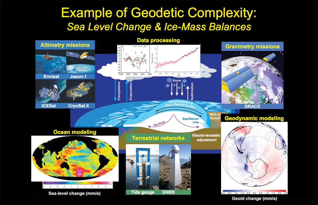
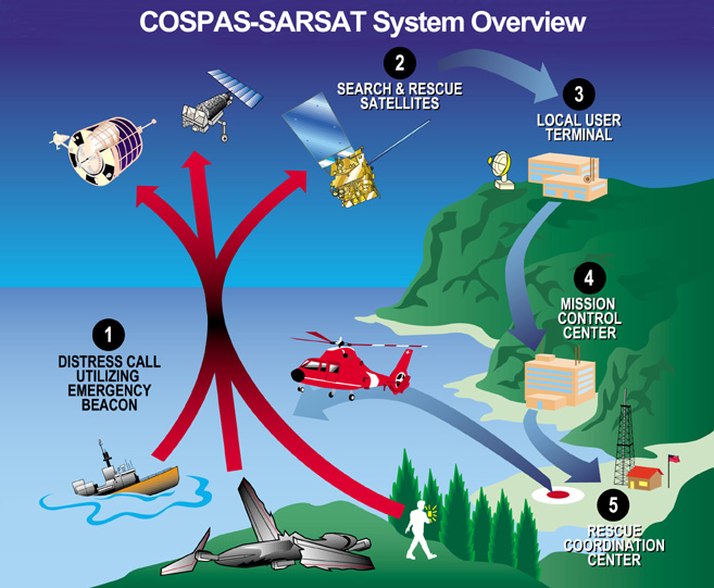

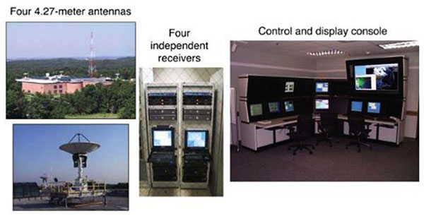

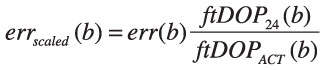
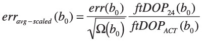
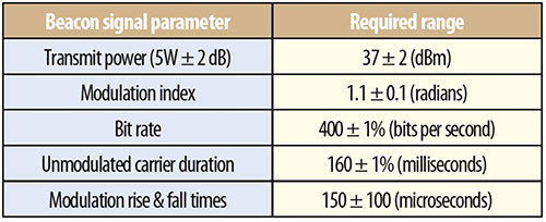
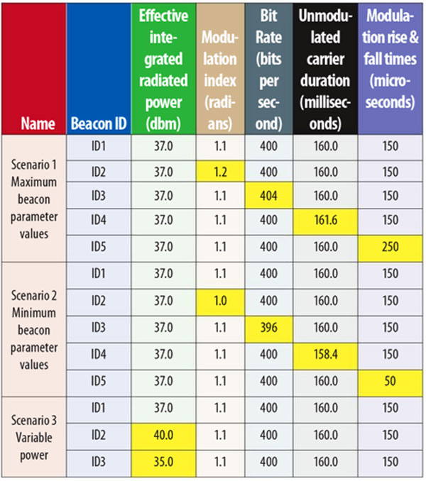
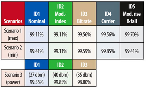
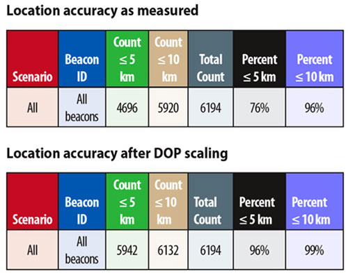
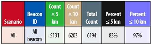
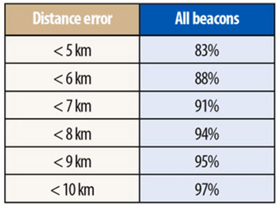
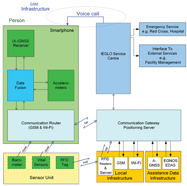
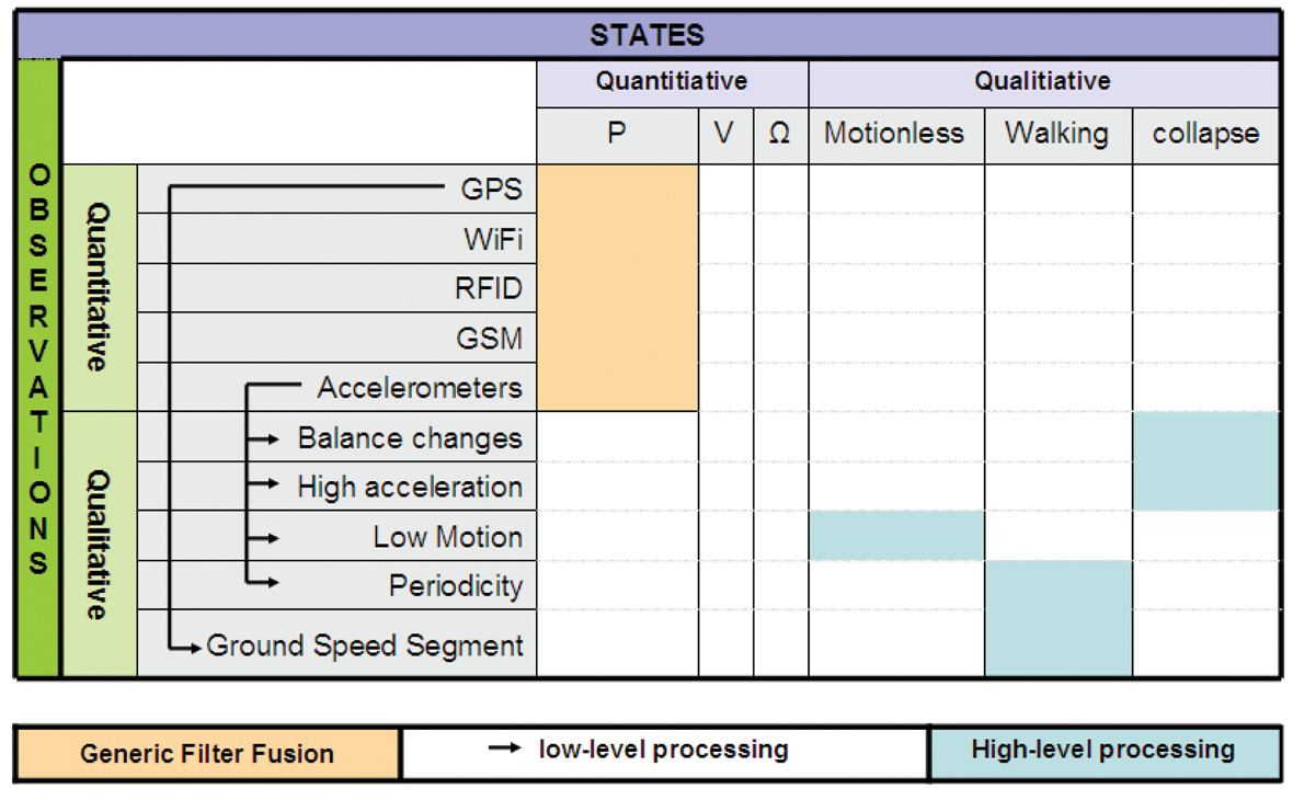
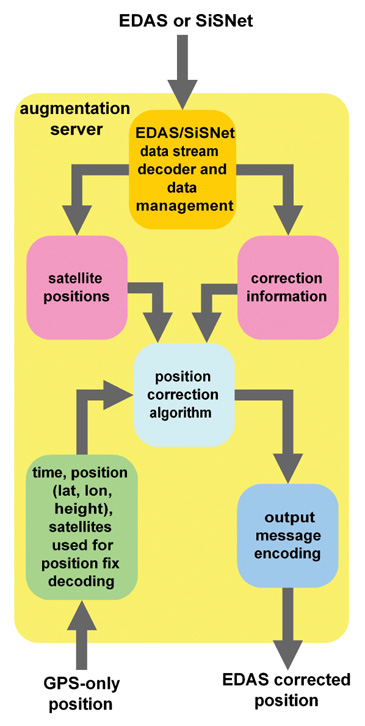
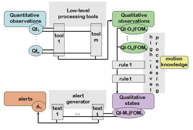
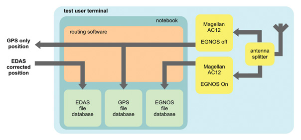
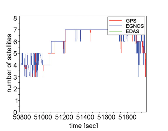
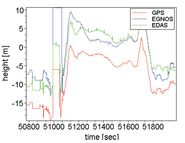
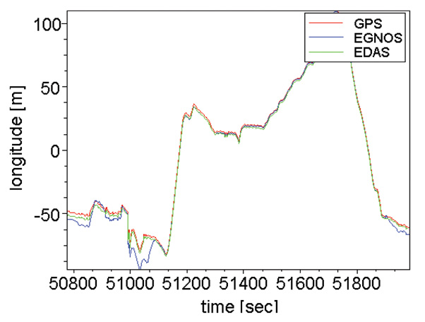
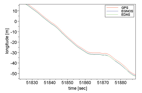
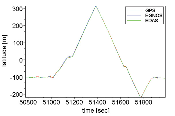
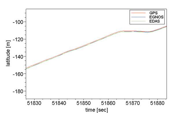
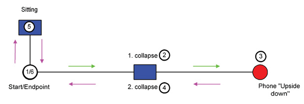
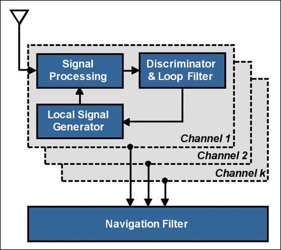
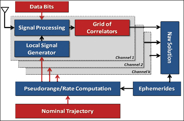
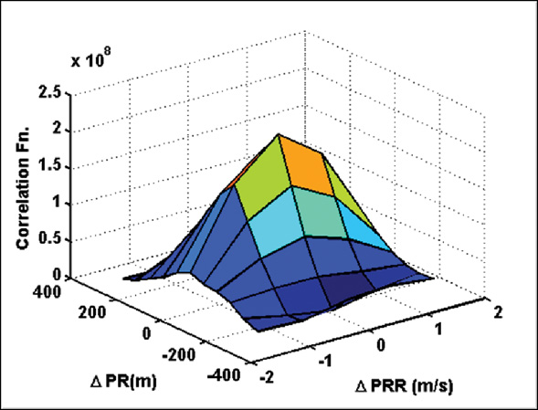

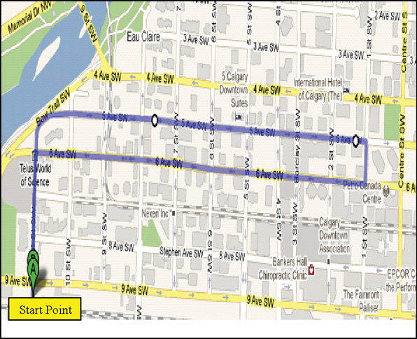
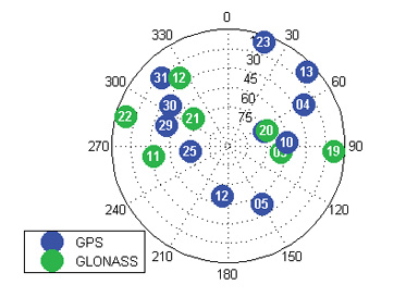
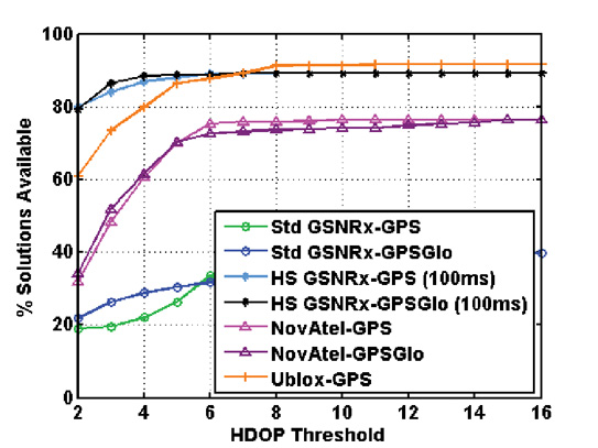
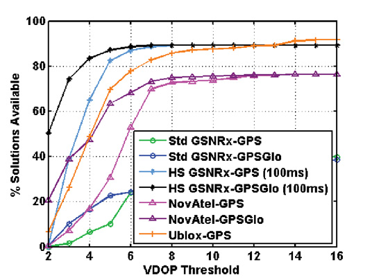
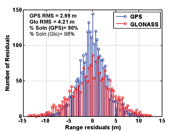
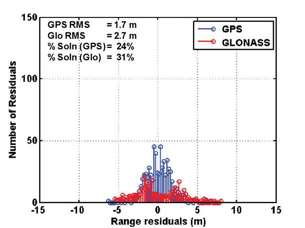
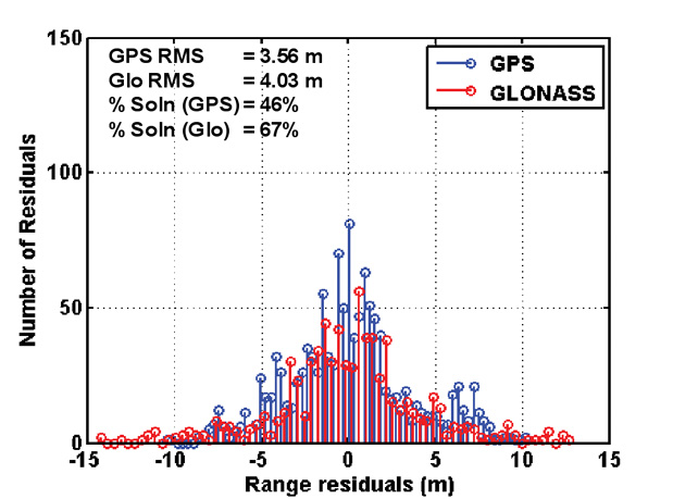
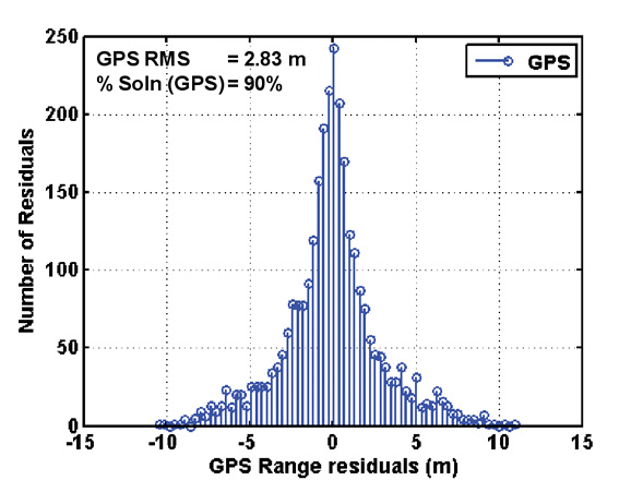
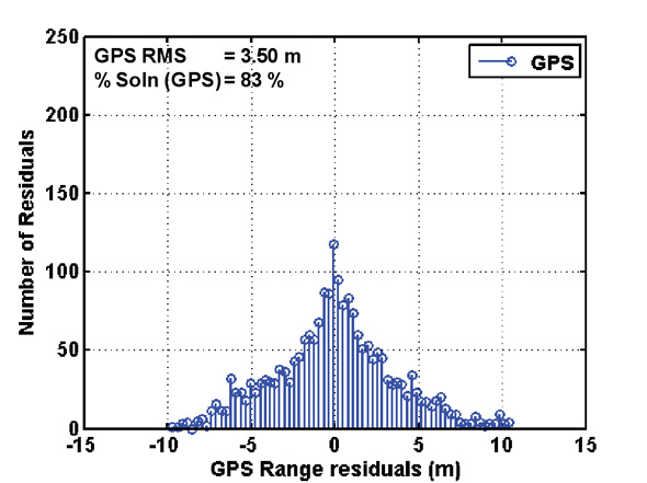
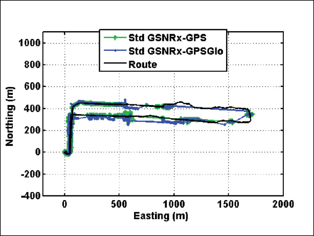
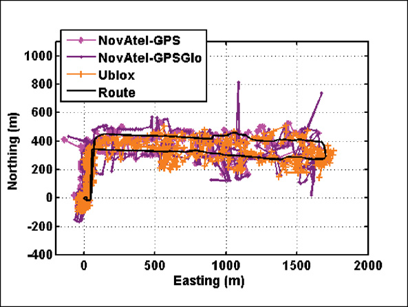
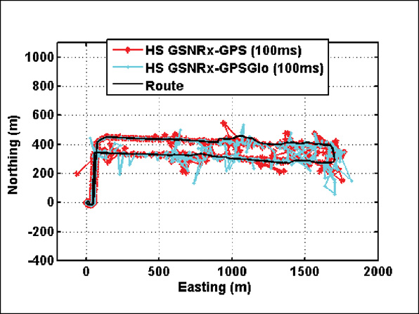
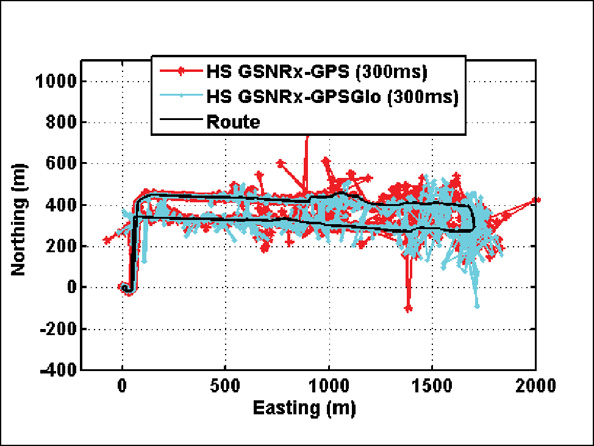
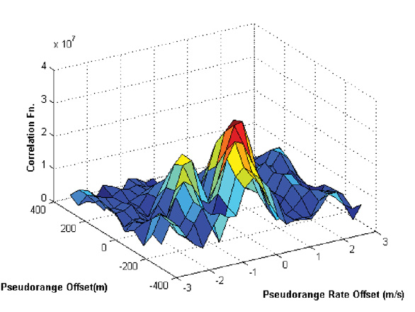


 Huntsville is the home of the original rocket scientists led by Werner von Braun, and home to the NASA Marshall Space Center and Redstone Arsenal. The city has become an extensive technology center with the Rocket Center as a focal point. If you visit, plan on a full day to see it all.


