Keynotes at February’s Inertial Sensors conference summarize initiatives to provide continuous, high-frequency and high-accuracy position spanning GPS outages or obstructions.
GPS-Free. Robert Lutwak, program manager at the U.S. Defense Advanced Research Projects Agency (DARPA), spoke on “Precise Robust Inertial Guidance for Munitions: Navigating in a GPS-free World.”
Over the past decade, the DARPA Micro-Technology for Position, Navigation, and Timing (micro-PNT) program developed low-CSWaP inertial sensors as a backup or “flywheel” PNT solution for GNSS augmentation, validation and holdover in obfuscated environments. New programs, such as the Precise Robust Inertial Guidance for Munitions (PRIGM) program, seek to ruggedize and deploy devices developed under micro-PNT and to extend the performance to support longer and more dynamic mission scenarios. In addition to maturing micro-electro-mechanical systems (MEMS) and atomic technologies developed under micro-PNT, PRIGM is exploring new sensing modalities and architectures, including those enabled by integrated photonics and by the tight integration of photonic and MEMS technologies.
Accuracy One-Thousandfold. Lutwak also gave an overview of DARPA’s new Atomic Clocks with Enhanced Stability (ACES) program. A technology challenge budgeted for up to $50 million, ACES’ goal is to design and build a new generation of palm-sized, battery-powered atomic clocks that perform up to 1,000 times better than the current generation — DARPA’s Chip-Scale Atomic Clock.
The new clocks must fit into a package about the size of a billfold and run on a mere quarter-watt of power. Success will require advances that counter accuracy-eroding processes in current atomic clocks, among them variations in atomic frequencies that result from temperature fluctuations and subtle frequency differences that can occur if the power shuts down and then starts up again.
“It will take a collaboration of teams with skill sets from diverse fields, including atomic physics, optics, photonics, microfabrication and vacuum technology, to achieve the unprecedented clock stability that we seek,” Lutwak said.
MEMS Transition. Stephen Breit, director of engineering for Coventor, gave his predictions for the “Future of the Commodity MEMS Inertial Sensor Design and Manufacturing.”
Emerging trends that could lead to disruptive changes include commoditization of MEMS process technology, consolidation of advanced semiconductor technology, More-than-Moore integration, and the Internet of Things (IoT). These trends motivate industry efforts toward a transition similar to the one that occurred in the CMOS industry: from integrated device manufacturers to a fabless/foundry business model.
This will require a design automation flow that provides a platform for process design kits (PDKs) that foundries can supply to their fabless customers.
Exploiting fingerprints, other smartphone features
Tiny irregularities in an Android or iPhone’s accelerometer can be turned into a unique signature to track users, Stanford researchers found in 2013. These flaws essentially fingerprint an individual smartphone and allow it to be traced. Highly focused activity since then, some of it summarized here, has advanced the frontiers of non-GPS tracking. Developments could prove interesting to privacy advocates, online marketers and law enforcement.
Security researcher Hristo Bojinov demonstrated how, in a matter of seconds, he induced his smartphone to give up its “fingerprints.” Code running on a website in the device’s mobile browser measured the tiniest defects in the device’s accelerometer, producing a unique set of numbers — exploitable to identify and track most smartphones. Marketers could use the ID the same way they use cookies to identify a particular user, monitor their online actions and target ads.
The research team was also able to identify phones using their microphones and speakers. They found they could produce a unique frequency response curve, based on how devices play and record a common set of frequencies.
Amplifiers and Oscillators. A team at the Technical University of Dresden developed a tracking method that exploits variations in the radio signal of cell phones. The collection of components such as power amplifiers, oscillators and signal mixers can all introduce radio-signal inaccuracies.
Bojinov and colleagues presented further work at the RSA Conference 2015, in “Sensor ID: Mobile Device Identification via Sensor Fingerprinting.” Among findings:
We have found ways to construct a device ID by sensor fingerprinting.
All the sensors’ fingerprints may sum up to enough bits to identify all devices.
It is hardware dependent.
It can be used by web application.
A related presentation stated that “this is only the beginning. Many more unexpected information leakages will be found in the coming years. Treat every app you install as having ‘root’ on the phone. And think twice before installing that ‘harmless’ game.”
Engineers at Robert Bosch GmbH in Germany focused on MEMS-based gyroscopes and showed via wafer-level measurements and simulations that it is feasible to use the physical and electrical properties of these sensors for cryptographic key generation, a key requirement for full rollout of the Internet of Things.
Teams from Virginia Tech and the University of Essex have published papers detailing similar approaches, basically turning this vulnerability into a tool. “We prove that device identification can be generated by using the accelerometer found in many pervasive devices,” wrote the Essex researchers. “Our experiments are based on a set of health sensors equipped with a MEMS accelerometer. Periodic readings are obtained from the sensor and analyzed mathematically and statistically to generate a stable ICMetric number.”
Alissa Fitzgerald aided in assembling this overview report.
Q: What is the “killer app” for professional use of drones? What UAV market sector will most powerfully drive adoption and influence new regulations?
Jan Leyssens Product Manager, SeptentrioA: The mapping market is opening up. On construction and mining sites, surveyors walk between dozers and dump trucks to create digital terrain models, a time-consuming and dangerous job, which drones can do more efficiently and safely. These jobs are performed in non-public areas, without significant risks or privacy concerns, facilitating public acceptance. Subsequently the potentially larger inspection market will open up. Drones provide an easy, safe way to inspect wind turbines or other installations that are difficult or dangerous to reach.
Tony Murfin Contributing Editor, Professional OEM & UAV, GPS WorldA: The agriculture industry seeks even greater Improvements in crop yields. GNSS systems in the cabs of combines/harvesters have already helped significantly, but drone use for crop-growth monitoring, data collection and pesticide-prescription application is the big breakthrough — once rules for large-scale low-level drone flight over farmland are approved. Ag will push for published rules just as hard as the movies, real-estate and all types of aerial survey for construction and utilities.
Eric Gakstatter Contributing Editor, GIS & UAV, Geospatial SolutionsA: Amateur photographers and hobbyists are where the volume is. The world’s largest UAV manufacturer now exceeds $1B annual revenue. Its growth is being driven by the hobby market. Commercial use of UAVs is a very small piece of the worldwide UAV market. The UAV market will be very similar to the GPS receiver market, just not at the same scale. The volume in the UAV consumer market will drive the technology (sensors, motors, software) that will benefit commercial UAV manufacturers.
A new version 2.12 of the BKG NTRIP Client (BNC) will be available on April 18.
Originally developed in cooperation of the Federal Agency for Cartography and Geodesy (BKG) and the Czech Technical University (CTU) with a focus on multi-stream real-time access to GNSS observations, the software has been substantially extended.
The BKG Ntrip Client is an open source multi-stream client program designed for a variety of real-time GNSS applications. It was primarily designed for receiving data streams from any NTRIP supporting broadcaster. The program handles the HTTP communication and transfers received GNSS data to a serial or IP port feeding networking software or a DGPS/RTK application. In previous years, BNC has been enriched with RINEX quality and editing functions.
BNC on a Mac system for static real-time precise point positioning with Google Maps, such as for early warning of natural hazards.
Its primary objective is the promotion of open standards as recommended by the Radio Technical Commission for Maritime Services (RTCM). Implemented RTCM messages comprise satellite orbit and clock corrections, code and phase observation biases, and the Vertical Total Electron Content (VTEC) of the ionosphere.
Beside its graphical user interface, the real-time software for Windows, Linux and Mac platforms now comes with complete command line interface and considerable post-processing functionality. RINEX Version 3 file editing and quality check with full support of Galileo, BeiDou and SBAS — besides GPS and GLONASS — are among the new features.
Comparison of satellite orbit/clock files in SP3 format is another new feature of BNC.
BNC version 2.12 now allows a simultaneous multi-station Precise Point Positioning (PPP) for real-time displacement-monitoring of entire reference station networks.
BNC version 2.12 generates RINEX version 3.03 observation and navigation files to support near real-time GNSS post processing applications. Whenever BNC starts to generate RINEX observation files, it first tries to retrieve information needed for RINEX headers from so-called public RINEX skeleton files (skl files), which are derived from site logs. Therefore, BKG provides the current system observation types (sot files) per station. From April 18 onward, the sot files with BDS frequency bands consistent to the definition in RINEX version 3.03 will be provided.
Old configuration files cannot be used without problems. Nevertheless, BNC 2.12 download is coming out with a large set of examples for all the different applications, which can be easily adapted introducing a valid user account.
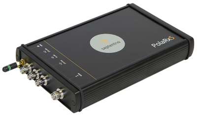
A new PolaRx5 Continuously Operating Reference Station (CORS) platform, offered by Septentrio Americas, is optimized for state departments of transportation (DOTs) and other real-time-kinematic (RTK) network operators.
The Septentrio PolaRx5 GNSS receiver.
The PolaRx5 CORS receivers can be purchased at special pricing by UNAVCO member organizations and affiliates. Septentrio has been selected by UNAVCO as the preferred vendor of CORS receivers under a multi-year agreement.
The PolaRx5 is powered by Septentrio’s AsteRx4 next-generation multi-frequency engine. It offers 544 hardware channels and supports all major satellite signals including GPS, GLONASS, Galileo and BeiDou, as well as regional satellite systems such as QZSS and IRNSS.
Septentrio’s Advanced Interference Mitigation (AIM+) technology enables the PolaRx5 to filter out both intentional and unintentional sources of radio interference, from narrowband signals over high-powered pulsed signals to chirp jammers and Iridium transmitters.
In addition, Septentrio’s patented APME+ multipath mitigation technology guarantees superior measurement quality by eliminating short-delay multipath errors without introduction of bias, the company said.
The PolaRx5 leverages Septentrio’s web interface and built-in Wi-Fi and Bluetooth interfaces to give users complete control and visibility of the receiver. The user interface integrates into existing network management systems. The web browser provides secure access to all receiver settings and status, data storage and firmware upgrades, as well as a built-in spectrum analyzer for system monitoring.
“The multi-constellation PolaRx5, with its powerful interference and multipath mitigation and new Web interface, is the ideal solution for DOTs to modernize their aging CORS installations to the newest GNSS technology,” said Neil Vancans, vice president of Septentrio Americas.
KVH Industries is developing a fiber optic gyro (FOG)-based, low-cost inertial sensor for self-driving cars.
The company also released a Developer’s Kit to assist design engineers with integrating FOG technology into driverless car control systems.
KVH’s high-precision FOG is key to a driverless car’s performance. In this photo, the red illumination represents light moving through the FOG’s optical circuit of coiled fiber; this circuit is the FOG’s sensing unit — it is mounted with power and processing electronics within a driverless car to provide precise data for the car’s navigation systems.
FOGs and FOG-based inertial measurement units (IMUs) are key parts of the sensor mechanisms that are essential for highly accurate autonomous car performance, KVH said. For example, FOGs provide precise azimuth measurements that an autonomous car’s logic processing unit and control systems need to determine motion through a curve.
An IMU — which includes FOGs and accelerometers in one compact package — also provides highly accurate 6-degrees-of-freedom angular rate and acceleration data to precisely track the position and orientation of the car even when GPS is unavailable, helping the car stay on course.
As a manufacturer of high-performance sensors and integrated inertial systems for defense and commercial guidance and stabilization applications, KVH Industries has experience in autonomous vehicle prototype programs and unmanned applications.
“Extremely precise heading based on fiber-optic gyro technology is absolutely essential for autonomous vehicle performance,” said Martin Kits van Heyningen, KVH’s chief executive officer. “This is something we learned from having been involved with more than a dozen driverless car development programs over the years.”
“What we are seeing now is that each driverless vehicle concept in development around the world is being designed in a unique way,” said Kits van Heyningen. “With so many different possibilities, developers can accelerate their progress by working with a proven technology such as KVH’s FOGs and FOG-based IMUs and leveraging our experience to ensure their success.”
Developer’s Kit. The new Developer’s Kit includes the user interface software and all components needed to connect a KVH FOG or FOG-based IMU to a computer to configure, analyze and test a unit. “The kit is designed to help engineers get up and running in minutes, making it easier to run diagnostics and accelerate their system development,” said Roger Ward, KVH’s director of FOG product development.
Driverless cars represent one of the fastest areas of autonomous-systems development. Transportation experts, automotive manufacturers and engineers alike predict that driverless cars will be commonplace soon.
An updated policy concerning automated vehicles will soon be published by the National Highway Traffic Safety Administration (NHTSA), which is part of the U.S. Department of Transportation. “The rapid development of emerging automation technologies means that partially and fully automated vehicles are nearing the point at which widespread deployment is feasible,” NHTSA said.
“We have successfully produced more than 90,000 fiber-optic gyros for an extensive range of unmanned applications, in part because of our ability to tailor size, performance, and cost to meet different design needs,” said Jeff Brunner, KVH’s vice president for FOG operations. “Controlling the entire FOG design and manufacturing process gives us that advantage, and makes it possible to produce a low-cost sensor when driverless cars enter full-scale production.”
KVH’s FOGs and FOG-based IMUs are in use in prototype programs not only for autonomous cars, but also for production programs for underwater unmanned vehicle navigation and rail/track geometry measurement systems, to name just a few.
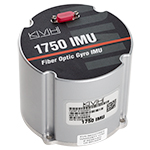
The KVH 1750 IMU.
In addition, KVH’s inertial products have been widely adopted for commercial applications such as land-based street mapping platforms, unmanned aerial systems, camera stabilization systems and remotely operated subsea systems.
As more and more programs and platforms use KVH’s inertial products, they are becoming the reference standards of the unmanned world. For example, KVH’s 1750 IMU was an integral part of 11 of the 23 humanoid robot finalists in last year’s DARPA Robotics finals, a competition designed to showcase robots capable of intervening for and even replacing humans in high-risk situations such as fires, earthquakes, and other natural disasters.
“Our IMUs and inertial sensors have already been used in a wide range of products and applications, and we know that it’s just the beginning,” said Kits van Heyningen. “We are thrilled to play a role in these exciting developments and emerging applications that are literally changing everyday life.”
Basic procedures and tools for ensuring GNSS-derived orthometric heights meet the project’s desired accuracy
To date, this series of columns has addressed the following topics: basic concepts of GNSS-derived heights, National Geodetic Survey’s (NGS) guidelines for establishing GNSS-derived ellipsoid heights (NGS 58), differences between hybrid and scientific geoid models, procedures and tools for detecting GNSS-derived ellipsoid height data outliers, and basic procedures for estimating GNSS-derived orthometric heights (NGS 59). These columns are meant to provide the reader with basic concepts, routines, and procedures for analyzing, evaluating, and estimating GNSS-derived heights.
As mentioned in the last column “Determining valid North American Vertical Datum of 1988 (NAVD 88) published heights is the most important process when using GNSS data and geoid models to estimate GNSS-derived orthometric heights.” In Part 5 (February 2016) of this series, we discussed NGS 59 guidelines and methods for evaluating the results of the GNSS project. It provided methods for evaluating the results of the project and identifying stations with valid NAVD 88 published heights. In this column, we will continue to analyze the changes in adjusted heights due to different height constraints and compare the results to the published NAVD 88 orthometric heights.
First, we need to discuss what should be considered an outlier when identifying valid NAVD 88 published heights to be used as constraints. According to NGS guidelines for performing GNSS adjustments, the rule of thumb for outliers are shifts greater than 2 cm horizontally and 4 cm vertically (see highlighted section in the box below). The guidelines also stated that “It is important to realize that this threshold is merely a ‘rule of thumb.’ For individual projects, unconstraining a station may be necessary if shifts are less than the ‘rule of thumb’ threshold, and in some cases it can remain constrained even if shifts slightly exceed the threshold.”
It is important to understand this concept because constraining the height of a station influences the heights of stations nearby that constraint. Also, not constraining a published height of a station will result in establishing a new height for that station which means it could be inconsistent with other published stations nearby that station. If the station had moved since the last time it was leveled to then not constraining the height is the appropriate action to take. However, if the shift is due to some other reason (such as a previous adjustment distribution correction, or ellipsoid and/or geoid issue), then constraining the height may be the appropriate action to take. Selecting constraints is not an exact science; as a matter of fact, at times, it appears to be more like an art or like solving an enigmatic puzzle.
Excerpt of NGS Adjustment Document, adjustment_guidelines.pdf, under section 5 titled Constrained Horizonal Adjustment.
As a general rule, if the adjusted values of the constrained coordinates of a station shift by more than 2 cm horizontally and/or 4 cm in height, its horizontal coordinates and/or ellipsoid height, respectively, should be unconstrained. Doing so means that the published values for the unconstrained passive control station will be updated by the adjusted values determined in the submitted survey (CORS coordinates will not be updated). This 2 cm horizontal and 4 cm vertical threshold is consistent with that used by NGS for updating published CORS coordinates, although for CORS this is done by NGS independent of individual campaign-style GPS projects. It is important to realize that this threshold is merely a “rule of thumb.” For individual projects, unconstraining a station may be necessary if shifts are less than the “rule of thumb” threshold, and in some cases it can remain constrained even if shifts slightly exceed the threshold. The decision to constrain or not constrain also depends on other factors, such as the statistics of the adjustment, residuals, shifts at other stations, and station accuracies. It requires judgment and should not simply be an automatic response to constrained station shifts.
The NGS guideline mentioned above is for horizontal coordinates and ellipsoid heights. The NGS guidelines under section 6 implies that the user should apply the same guidelines for shifts between GNSS-derived orthometric heights and published NAVD 88 orthometric heights (see highlighted section in the box below). The guidelines also recommend that the user analyze the shifts of stations near each other to determine if stations nearby each other are shifting consistently or if one of the station’s value appears to be an outlier (see underlined section in box below).
Excerpt of NGS Adjustment Document, adjustment_guidelines.pdf, under section 6 titled Vertical Adjustment (Free and Constrained).
SECTION 6, VERTICAL ADJUSTMENTS (FREE AND CONSTRAINED)
6-1. Create the vertical free Afile (Afilevf). Fix one position and one published orthometric height. They can be from the same station or different stations (e.g., good horizontal position in one CC record for a CORS, good OH in separate CC record for a bench mark). Leaving column 77 of the CC record blank indicates the record contains an orthometric height value. Standard deviations of the constrained coordinates and heights should NOT be entered (i.e., columns 15-32 of the CC record should be blank).
Include the VS record from the horizontal constrained Afile.
70-76 Height, units of millimeters (integer)
77-77 Height Code blank — orthometric height
6-2. Run Adjust with minimum constraints. Input: Bfileght, Afilevf, Gfile, Output: adjvf.out, Bfilevf
Assuming the adjustment ran to completion, the statistics of this run will be identical to those of the horizontal free adjustment. Check adjvf.out for big shifts between published and free-adjusted heights.
It would be helpful to compute the shifts between the results of the vertical free adjusted and the published heights. Additionally, plot these shifts on a project sketch to determine if several heights near each other are shifting consistently or a height appears to be an outlier and therefore should not be used as control. For inconsistent shifts use resources available such as recovery notes, photographs, and rubbings of the mark. Possible causes could include movement, an unintended mark was observed such as the underground mark instead of the surface mark, or occupying a reference mark rather than the parent station. Look for inconsistent shifts as opposed to areas where the shifts, even high shifts, are consistent. Likewise, look at the geoid heights to ensure they are consistent. If no cause for the shift can be found, the orthometric height may need to be readjusted.
6-3. Create the vertical constrained Afile (Afilevc). Constrain all previously adjusted orthometric heights as indicated above and one NAD 83 adjusted position. The same comments about CC records apply. All GPS-derived Ht Mod heights should be constrained along with bench marks. For ht mod stations the datasheet will read:
HT_MOD – This is a Height Modernization Survey Station.
Include the VS record with its appropriate values.
6- 4. Run Adjust with vertical constraints. Input: Bfilevf, Afilevc, Gfile, Output: adjvc.out, Bfilevc
Run PrePlt2 to list and sort the residuals. Investigate observations with large shifts or residuals to see if any heights should be readjusted. Apply the same rule as in the horizontal constrained adjustment: no rejections due to constraints. Free any heights in question and rerun as a test. Note the differences between the published and readjusted heights obtained from the vertical constrained adjustment. Consider the requirements of the project before deciding whether to readjust additional points. Save the output Bfile from the final constrained vertical adjustment.
In Part 5, I highlighted a potential issue at station Phaniel. I’ve included the diagrams and tables from Part 5 that depicts the differences between GNSS-derived orthometric heights from a minimum-constraint adjusyment (using GEOID12B and xGeoid15b) and the published NAVD 88 height values (see figures 1-4, and tables 1-2). Looking at figures 1 and 2, there are several large differences between closely spaced constraints when using the hybrid geoid model – Phaniel, Buffalos 2, V 49, and Row 9. As stated in Part 2, the user should compute the results using both the hybrid and the scientific geoid models. Figures 3 and 4 depict the differences using the scientific geoid model xGeoid15b. Notice that the large differences between Phaniel and Buffalo 2 decreased from 4.9 cm using GEOID12B to 0.7 cm using xGeoid15b. However, the larger relative difference between Phaniel and V 49 (3.8 cm) and ROW 9 (5.2 cm) still exists. Also, the difference between Buffalo 2 and V 49 is large (3.1 cm), and Buffalo 2 to Row 9 is large (4.5 cm), but the difference between V 49 and Row 9 is less than 2 cm. The neighbor stations of Row 9 all seem to agree within a couple of centimeters indicating that Buffalo 2 may be a station that needs further investigation.
Figure 1. [Figure 3 from Part 5] Diagram depicting differences between GNSS-derived orthometric heights from a Minimum-Constraint Adjustment (using GEOID12B) and published NAVD 88 height values (units=cm).Figure 2. [Figure 4 from Part 5] Diagram depicting differences between GNSS-derived orthometric heights from a Minimum-Constraint Adjustment (using GEOID12B) and published NAVD 88 height values (units=cm).
Figure 3. [Figure 5 from Part 5] Diagram depicting differences between GNSS-derived orthometric heights from a Minimum-Constraint Adjustment (using xGeoid15b) and published NAVD 88 height values (units=cm).Figure 4. [Figure 6 from Part 5] Diagram depicting differences between GNSS-derived orthometric heights from a Minimum-Constraint Adjustment (using xGeoid15b) and published NAVD 88 height values (units=cm).
Next we need to look at the adjusted ellipsoid heights from a minimum-constraint solution compared to the published ellipsoid heights. This procedure was decribed and demonstrated in Part 4. Figure 5 is plot of adjusted ellipsoid height minus published NAD 83 (2011) ellipsoid heights for stations near Phaniel. Figure 5 indicates that the adjusted ellipsoid heights at Buffalo 2, Phaniel, and V 49 all agree within 2 cm. As a matter of fact, Buffalo 2 and Phaniel agree to better than 1 cm from the NAD 83 (2011) published heights. This is an indication that the orthometric height of station Phaniel may be an outlier and should not be constrained. The leveling network in the area requires investigation to validate this conclusion. This will be addressed in a future column. Looking at Tables 1 and 2, two other stations, stations Plaza and Row 3, have large differences between the GNSS-derived orthometric heights from a minimum-constraint adjustment and the published NAVD 88 heights, and they should be investigated.
Figure 5. Plot of adjusted ellipsoid height minus published NAD 83 (2011) Ellipsoid Heights for Stations near Phaniel (the number is the difference for that particular station; units = cm).Table 1. Differences between GNSS-derived orthometric heights from a minimum-constraint adjustment (using GEOID12B) and published NAVD 88 heights (GEOID12B results sorted and highlighted).Table 2. Differences between GNSS-derived orthometric heights from a minimum-constraint adjustment (using xGeoid15b) and published NAVD 88 heights (xGeoid15b results sorted and highlighted).
Figure 6 is a diagram depicting differences between GNSS-derived orthometric heights from a minimum-constraint adjustment using GEOID12B and published NAVD 88 heights surrounding station Plaza. The user should notice that the relative difference in height changes between Plaza and 37 DRD is -3.8 cm (-2.5 – 1.3) and between Plaza and Fifth it is -3.2 cm (-2.5 – 0.7). This is an indication that there is a potential issue with station Plaza. Next, we need to compute the results using xGeoid15b. Figure 7 is a plot of the differences surrounding station Plaza using xGeoid15b. Figure 7 shows that station Plaza outliers relative to station 37 DRD and Fifth are exactly the same, i.e., -3.8 cm (-3.2 – 0.6) and -3.2 cm (-3.2 – 0.0) respectively. Something interesting to note is that station J 181 difference decreased from 2.1 cm using GEOID12B (see figure 6) to 1.1 cm using xGeoid15b (see figure 7). Once again, this is a reason why users should use both the hybrid geoid model and the scientific geoid model when analyzing GNSS-derived orthometric heights.
Figure 6. (More Detail at Station Plaza) Diagram depicting differences between GNSS-derived orthometric heights from a Minimum-Constraint Adjustment (using GEOID12B) and published NAVD 88 height values (units=cm).
Figure 7. (More Detail at Station Plaza) Diagram depicting differences between GNSS-derived orthometric heights from a Minimum-Constraint Adjustment (using xGeoid15b) and published NAVD 88 height values (units=cm).
The other station to investigate based on the large difference in table 2 is station Row 3. Figure 8 is a diagram depicting the differences near station Row 3 using GEOID12B. Notice that the difference at Row 3 is considerably less than the 4 cm; however, the relative difference between Row 3 (-2.7 cm) and station 384 JAS (0.2 cm) is -2.9 cm. This doesn’t seem too large but computing the results using xGeoid15b indicates something different. Figure 9 is a plot of the differences using the scientific geoid model xGeoid15b. Notice that the difference at station Row 3 increased to -3.8 cm and the relative difference between Row 3 and 384 JAS is -3.9 cm. Note, this again emphases the importance of using both the hybrid and scientific geoid models when analyzing GNSS-derived orthometric heights. This large relative difference is an indication that the height of station Row 3 may not have a valid NAVD 88 published height and should be further investigated before constraining the height in the final adjustment.
Figure 8. (More Detail at Station Row 3) Diagram depicting differences between GNSS-derived orthometric heights from a Minimum-Constraint Adjustment (using GEOID12B) and published NAVD 88 height values (units=cm).Figure 9. (More Detail at Station Row 3) Diagram depicting differences between GNSS-derived orthometric heights from a Minimum-Constraint Adjustment (using xGeoid15b) and published NAVD 88 height values (units=cm).
After analyzing the differences between GNSS-derived orthometric heights from a minimum-constraint adjustment and published NAVD 88 heights to help identify potential outliers, the user can perform a constrained adjustment holding the published height values as constraints. The user should ensure that a constraint does not significantly affect the adjusted heights of neighboring stations. To understand the effects of the constraints on the heights of stations that are not constrained, the user can plot the changes in adjusted heights between the constrained adjustment and the minimum-constraint adjusted heights (with a bias removed). As mentioned in Part 5, any constraint can be used to obtain a minimum-constraint solution so removing a bias based on the differences between the published height values and the adjusted height values obtained from a solution constraining one published height is appropriate. Figure 10 is a plot that depicts the differences between the adjusted heights from an adjustment with all published NAVD 88 height values constrained and the adjusted heights values from the minimum-constraint adjustment. Figure 10 highlights the large relative changes of closely spaced stations such as between Phaniel (-2.8 cm) and Open (-0.6 cm). This means that the constraint at station Phaniel has changed the relative height difference between station Phaniel and station Open by 2.2 cm. This is a large change when you trying to obtain 2 cm heights. Another method to see the effect of the constraints is by plotting the changes in “dU” residuals between the constrained adjustment and the minimum-constraint adjustment. Figure 11 is a plot of the differences in vector “dU” residuals between the constrained adjustment (with all published heights constrained) and the minimum-constraint adjustment.
Figure 10. Diagram depicting differences between GNSS-derived orthometric heights from a Constrained Adjustment (All Published Heights Constrained) minus Minimum-Constraint Adjustment (using GEOID12B) – units=cm.
Looking at figure 11, the user can quickly see that constraining station Phaniel has changed the three vectors associated with Phaniel by 1.9 cm, 2.1 cm, and 2.3 cm. This means that the observed vectors were changed by 2 cm to be consistent with the constraint at Phaniel. This could have an impact on a surveyor performing leveling between these two stations. The analyst should now perform an adjustment not constraining the stations identified as potential outliers. At this moment, in this study, stations Phaniel, Plaza, and Row 3 are considered questionable and their heights will not be constrained.
Figure 11. Diagram depicting differences between dU Residuals of Vectors from a Constrained Adjustment (All Published Heights Constrained) minus Minimum-Constraint Adjustment (using GEOID12B) – units=cm.
Figure 12 is a diagram depicting the differences between the GNSS-derived orthometric heights from a constrained adjustment were the height values of stations Phaniel, Plaza, and Row 3 were not constrained. Figure 13 is a diagram depicting the differences between the dU residuals of baselines from the constrained adjustment with heights of stations Phaniel, Plaza, and Row 3 not constrained and the dU residuals from the minimum-constraint adjustment. Figures 14 and 15 provide more detail of the changes in residuals near station Phaniel. Figure 14 depicts the differences when all NAVD 88 heights are constrained and figure 15 depicts the differences when the suspected stations (Phaniel, Plaza, and Row 3) are not constrained. Comparing figures 14 and 15 clearly show that by constraining station Phaniel, the relative differences between station Phaniel and its neighbors are adversely effected by the constraint. For example, the difference in dU residuals between Phaniel and Brown Az Mk decreased from 2.3 cm to -0.2 cm resulting in a 2.5 cm relative height change.
Figure 12. Diagram depicting differences between GNSS-derived orthometric heights from a Constrained Adjustment (Three Stations Unconstrained) minus Minimum-Constraint Adjustment (using GEOID12B) – units=cm.Figure 13. Diagram depicting differences between dU Residuals of Vectors from a Constrained Adjustment (Three Stations Unconstrained) minus Minimum-Constraint Adjustment (using GEOID12B) – units=cm.Figure 14. (More Detail at Station Phaniel) Diagram depicting differences between dU Residuals of Vectors from a Constrained Adjustment (All Stations Constrained) minus Minimum-Constraint Adjustment (using GEOID12B) – units=cm.Figure 15. (More Detail at Station Phaniel) Diagram depicting differences between dU Residuals of Vectors from a Constrained Adjustment (Three Stations Unconstrained) minus Minimum-Constraint Adjustment (using GEOID12B) – units=cm.
As previously mentioned, station Plaza is another station with a large difference between the adjusted height from the minimum-constraint adjustment and its published height (see tables 1 and 2). Constraining station Plaza results in very large dU residuals between station Plaza and station 37 DRD, i.e, 3.7 cm over a distance of 1.1 km (see figure 16). By not constraining the height of station Plaza the dU residuals on the vector between station Plaza and station 37 DRD changed from 3.7 cm to 0.4 cm (see figure 17). Also, the dU residuals on the vector between station College and station Hudson changed from -1.8 cm to -0.1 cm, and dU residuals on the vector between station Dorsett and station Hudson changed from -1.7 cm to 0.2 cm. The distance between Dorsett and Hudson is 1.2 km. The allowable section closure for second-order, class 2 leveling in 1.2 km is 0.88 cm. If a user wanted to check their leveling work using these two stations they may not check within the allowable because of the large distribution correction applied to the adjusted heights due to constraining the height of station Plaza.
Figure 16. (More Detail at Station Plaza) Diagram depicting differences between dU Residuals of Vectors from a Constrained Adjustment (All Stations Constrained) minus Minimum-Constraint Adjustment (using GEOID12B) – units=cm.Figure 17. (More Detail at Station Plaza) Diagram depicting differences between dU Residuals of Vectors from a Constrained Adjustment (Three Stations Unconstrained) minus Minimum-Constraint Adjustment (using GEOID12B) – units=cm.
Next, the user should look at the differences in ellipsoid heights between minimum-constraint adjustment and published NAD 83 (2011) ellipsoid heights in the area of station Plaza (see figure 18). Station Plaza did not have a published NAD 83 (2011) ellipsoid height but the closest two stations (Dorsett and Salisbury CORS ARP) both agree within 0.6 cm of the published NAD 83 (2011) ellipsoid heights. This is a good sign tht the ellipsoid heights meet the desired accuracy but doesn’t help to explain the large difference at station Plaza.
Figure 18. (More Detail at Station Plaza) Diagram depicting differences between Adjusted GNSS-Derived Ellipsoid Heights (with average bias removed) minus Published NAD 83 (2011) Ellipsoid Heights (units=cm).
The third station with a large relative difference highlighted in table 2 is station Row 3. Figures 19 and 20 provide more detail of the changes in residuals near station Row 3. Notice that the dU residual of the vector between station Railroad and Magna changed from 1.5 cm to 0.1 cm when the height of Row 3 is not constrained. The distance between the two stations is 4 km so the effect of constraining this station is not really significant. It should be noted that one of the reasons it’s being investigated is because of the large relative difference between Row 3 and station 384 JAS using xGeoid15b (-3.9 cm, see figure 9). Figure 21 is a plot of the differences in ellipsoid heights obtained from the minimum-constraint adjustment and their published NAD 83 (2011) ellipsoid heights in the vicinity of station Row 3. Station Row 3 does not have a published NAD 83 (2011) ellipsoid height but all of the stations surrounding the station are less than 2 cm. There does not appear to be any large outliers compared with the published ellipsoid heights in the area. Once again, this means that the next step in the process is to investigate the leveling network in the area.
Figure 19. (More Detail at Station Row 3) Diagram depicting differences between dU Residuals of Vectors from a Constrained Adjustment (All Stations Constrained) minus Minimum-Constraint Adjustment (using GEOID12B) – units=cm.Figure 20. More Detail at Station Row 3) Diagram depicting differences between dU Residuals of Vectors from a Constrained Adjustment (Three Stations Unconstrained) minus Minimum-Constraint Adjustment (using GEOID12B) – units=cm.Figure 21. (More Detail at Station Row 3) Diagram depicting differences between Adjusted GNSS-Derived Ellipsoid Heights (with average bias removed) minus Published NAD 83 (2011) Ellipsoid Heights (units=cm).
Up to this point we have analyzed changes in adjusted heights due to different constraints and compared the results to the published NAVD 88 GNSS-derived orthometric heights to identity stations that should be constrained in the final adjustment. As one can see, performing GNSS-derived orthometric height adjustments is more like an art than an exact science. There are a lot of variables and unknowns. Every constraint has an influence on the final set of adjusted heights. Determining this effect and the consequences of selecting an invalid constraint has been described in this column.
When incorporating new geodetic data into the National Spatial Reference System, it is important to maintain consistency between neighboring stations. If the published height of a station is not constrained, it will be superseded by the newly adjusted height. If the station has moved since the last time its height was established then superseding the height is the appropriate action to take. If the difference is due to some other reason such as the results of a previous adjustment distribution correction then superseding the height may not be the appropriate action to take.
In my next column, Part 7, we will look at the design of the NAVD 88 leveling network and published heights in the area to help determine the final set of stations to constrain.
PoLTE Corporation has developed technology that harnesses the global long-term evolution (LTE) deployment to provide accurate and reliable location data.
Unlike localized solutions, such as Wi-Fi and Bluetooth, PoLTE’s technology leverages its Positioning over LTE (PoLTE) Macro software to achieve precision of 2 to 6 meters. The technology makes use of the sounding reference signals (SRS) embedded in an LTE handset user’s transmission. Using adapted radar location techniques, it converts portions of the LTE uplink signal into a probe signal.
The technology enables mobile network operators to deliver highly accurate location data to customers in indoor and outdoor environments.
Traditional macro cell location methods require at least three towers to see the user device to locate the device with precision. Historically, single tower deployments were limited in accuracy to the width of the sector created by the 120-degree antenna that was serving the user device. For example, at a distance of 1.5 kilometers from a base station, the cross range precision would be 4,000 meters. PoLTE Macro can improve the precision to less than 2 meters.
The benefits to leveraging network-based positioning include speed, flexibility, accuracy and data analytics. Customers for the technology include machine-to-machine and Internet of Things technologies, mobile advertising, crowd and customer tracking, and public safety.
INRIX Inc., a connected car services and movement analytics company, has released a redesigned version of INRIX Traffic for iOS and Android.
INRIX Traffic is a next-generation navigation and traffic app that learns user preferences to take the guesswork out of driving. The app integrates with a user’s calendar and learns their driving habits to create a personalized itinerary that includes automatic alerts, anticipated trips, favorite destinations and preferred routes.
Available worldwide now in the Apple App Store and Google Play, INRIX Traffic learns routines and preferences as users go about their day. INRIX Traffic adds favorite places automatically instead of requiring users to spend time inputting destinations such as home, work or school.
Based on learned activities, it creates a daily, driver-specific itinerary of anticipated trips, as well as frequent and preferred routes. By accessing calendar information on a mobile device, the app also adds events with addresses to the daily driving itinerary.
Unlike other driving apps that can provide inaccurate traffic and incidents based purely on consumer input, INRIX Traffic uses a massive crowd-sourced network of more than 275 million connected cars and devices to offer accurate map and real-time information.
INRIX Traffic proactively monitors road conditions to alert drivers of ideal departure times, changes to arrival times and optimal routes to frequent or scheduled destinations based on real-time traffic.
“We designed INRIX Traffic with one specific vision: To help drivers move through their daily lives as quickly and efficiently as possible. The app uses our advanced traffic science to make even routine trips easier,” said Bryan Mistele, president and CEO, INRIX. “Users want an app that is accurate, personalized and smart enough to work proactively for them — so we’ve integrated several highly advanced technologies into one all-encompassing app.”
INRIX Traffic uses the crowd-sourced and free OpenStreetMap (OSM) for map data. By leveraging the power of user-generated content around the world, OSM can quickly adapt to the ever-changing road network. Using OSM enables INRIX to bring a high-quality map and turn-by-turn navigation to users at no cost and without advertisements. In addition to reporting incidents along their route including accidents, police activity and road hazards, INRIX Traffic users can send map feedback directly from the app.
INRIX Traffic is powered by the same technologies the company delivers to its automotive customers such as Audi, BMW, Lexus, Mercedes-Benz and Porsche. These connected car services include real-time and predictive traffic, off-street parking information and drive-time alerts. INRIX will continue integrating features from its product portfolio into future versions of INRIX Traffic.
INRIX Traffic is available in eight languages in 16 countries across North America and Europe, including Canada, France, Germany, Spain, United Kingdom and United States, with additional countries coming soon.
The app is built on Autotelligent, the company’s new software development kit and integrated cloud platform that provides machine learning and route monitoring. Autotelligent can be integrated into products in multiple industries such as automotive, enterprise and mobile.
Omata is introducing a new analog GPS speedometer that displays the information most essential to the activity in a classic form.
Starting with cycling, Omata introduces the Omata One speedometer, designed to complement and maintain the purity of the ride as well as look beautiful on the bike.
On the inside of the speedometer is a GPS computer that records with high precision so that cyclists can at download their activity data to their preferred training applications or sites.
On the outside Omata One has a legible and mechanical analog movement that shows riders the speed, distance, ascent and time. The company’s first product displays only these four, core pieces of information so the cyclist can focus on the ride.
“Everything about your bike should be as pure, inspiring and beautiful as the ride itself,” said the Omata team in a press release. “We are a team of ruthlessly dedicated and committed product makers who believe great design and meaningful products come more from what you leave out, rather than what you add in.”
The Omata One speedometer will launch on Kickstarter on April 5 with estimated delivery of the first product in February 2017. Omata One will subsequently be available through omata.com.
A new market report, “Unmanned Aerial Vehicle (UAV) Payloads & Subsystems Market Report 2016-2026,” is being offered by Visiongain. According to the 302-page report, the global UAV payloads and subsystems market is set to grow as nations seek to sustain and enhance their capabilities as the probability for symmetric warfare increases.
Communications and navigation UAV payloads and subsystems is one of four submarkets analyzed in the report, along with EO/IR, radar and intelligence.
The report answers questions such as:
What are the future prospects for the overall UAV payloads and subsystems market?
Who are the key players within the UAV payloads and subsystems market?
What are the drivers and restraints underpinning the UAV payloads and subsystems market?
Where are the most promising business opportunities by region, by technology and end use application?
Global drone manufacturers 3DR, DJI, GoPro and Parrot today are forming the Drone Manufacturers Alliance, a coalition intended to serve as the voice for drone manufacturers and their customers across civilian, governmental, recreational, commercial, nonprofit and public safety applications.
“We will advocate for policies that promote innovation and safety, and create a practical and responsible regulatory framework,” said Kara Calvert, director of the Drone Manufacturers Alliance. “There are significant economic and social benefits to drone operations in the U.S., and industry must work with policymakers to ensure a safe environment for flying.
“The Drone Manufacturers Alliance believes a carefully balanced regulatory framework requires input from all stakeholders and must recognize the value and necessity of continued technological innovation. By highlighting innovation and emphasizing education, we intend to work with policymakers to ensure drones continue to be safely integrated into the national airspace.”
The European Satellite Navigation Competition (ESNC) — the largest international competition for the commercial use of satellite navigation — is once again looking for outstanding ideas and business models. Renowned institutions and regional partners are set to award prizes worth a total of €1 million in more than 25 categories.
The deadline for submissions is June 30.
“In our modern, data-driven economy, satellite navigation is a crucial technology that facilitates constant and reliable object localisation — the bedrock of the Internet of Things,” states an ESNC press release. “Since 2004, the ESNC has evolved into a leading fixture in the New Space Economy by provided a public innovation platform for turning promising ideas into market-ready products.
“Each year, the competition unveils new trends and more than 500 business ideas. It has already awarded prizes to more than 270 winners over the years, which represent just a fraction of the nearly 3,500 innovative concepts submitted by over 10,000 total participants.
“Through a one-of-a-kind network that includes the ESA Business Incubation Centres and other incubators across Europe, the ESNC plays a decisive role in the realization of these ideas by supporting the foundation of startups and creating high-tech jobs.”
The unmanned aerial vehicle (UAV) trend has also emerged in the ideas submitted to the ESNC, which selected a drone application — Poseidron — as its overall winner for the first time in 2015. Developed by the Spanish startup Sincratech Aeronautics, this multicopter is equipped with infrared cameras and uses the European positioning service EGNOS to save lives at sea.
The Poseidron concept UAV.
This year’s winners will take home prizes worth a total of €1 million and be welcomed into the ESNC’s leading innovation network for global satellite navigation systems. Along with cash, the various prize categories on offer primarily include technical, business-related, and legal support in realising the winning business models.
A jury of international experts from the realms of research and industry will also evaluate the winners of all the categories to select an overall winner, who will be revealed at the annual awards ceremony.
Those who enter the ESNC also stand to benefit greatly from the opportunity to work closely with leading institutions and regional partners. The ESNC is geared towards individuals and teams from companies, research facilities, and universities around the world. Those interested can enter the competition from 1 April to 30 June 2016 at www.esnc.eu.
In ESNC 2016, prizes are sponsored by the following partner regions and institutions: the European Space Agency (ESA), the German Aerospace Center (DLR), the German Federal Ministry of Transport and Digital Infrastructure (BMVI), and the Horizon 2020 project BELS. Prototypes can also be entered into the GNSS Living Lab Challenge.
The University Challenge, meanwhile, is explicitly designed for students and university research assistants. This year’s confirmed partner regions are: Asia, Austria, Baden-Württemberg, Bavaria, the Czech Republic, Flanders, France, Galicia, Hesse, Ireland, Israel, Lithuania, Madrid, the Netherlands, Norway, Poland, Romania, Sweden, Switzerland, the United Kingdom and Valencia.
The official website offers all the relevant information on the prizes, partners, and terms of participation involved in the ESNC.
ESNC and Copernicus Masters Info Day is scheduled for June 2 at the European Space Solutions conference in The Hague. Those interested will also have further opportunities to meet the ESNC’s organisers and their partners at numerous regional kickoff events across Europe in April and May.


![Figure 1. [Figure 3 from Part 5] - Diagram depicting differences between GNSS-derived orthometric heights from a Minimum-Constraint Adjustment (using GEOID12B) and published NAVD 88 height values (units=cm).](https://stage.globalpositioningnews.com/wp-content/uploads/2016/04/Rowan-County_Newsletter_5_3.jpg)
![Figure 2. [Figure 4 from Part 5] - Diagram depicting differences between GNSS-derived orthometric heights from a Minimum-Constraint Adjustment (using GEOID12B) and published NAVD 88 height values (units=cm).](https://stage.globalpositioningnews.com/wp-content/uploads/2016/04/Rowan-County_Newsletter_5_4.jpg)
![Figure 3. [Figure 5 from Part 5] - Diagram depicting differences between GNSS-derived orthometric heights from a Minimum-Constraint Adjustment (using xGeoid15b) and published NAVD 88 height values (units=cm).](https://stage.globalpositioningnews.com/wp-content/uploads/2016/04/Rowan-County_Newsletter_5_5.jpg)
![Figure 4. [Figure 6 from Part 5] - Diagram depicting differences between GNSS-derived orthometric heights from a Minimum-Constraint Adjustment (using xGeoid15b) and published NAVD 88 height values (units=cm).](https://stage.globalpositioningnews.com/wp-content/uploads/2016/04/Rowan-County_Newsletter_5_6.jpg)


 The European Satellite Navigation Competition (