Aeris is partnering with Isotrak Ltd. to provide improved cellular connectivity and data analytics for Isotrak’s global customers.
By leveraging Aeris’ machine-optimized and patented AerCore IoT and M2M network, AerPort connectivity platform and AerVoyance IoT and M2M analytics platform, Isotrak has added advanced capabilities to its 3iS FleetVision solution, part of its real-time ATMSi (Active Transport Management System) fleet management system. Isotrak can now provide business intelligence data to provide retailers and manufacturers with a full view of their transportation ecosystem — including their own fleets as well as those of third-party suppliers.
The collaboration between Aeris and Isotrak will provide customers with a reliable mobile network optimized to meet the demands that IoT/M2M solutions for fleet management creates, while providing actionable visibility and measurement into the performance of vehicles and drivers through data analytics. Isotrak’s integrated supply-chain solutions depend on accessing near real-time data with robust alerting and reporting capabilities, which Aeris is able to deliver through its carrier-agnostic network.
“Our fleet management system provides data for a total vision of a fleet manager’s transportation ecosystem. We wanted to ensure reliable connectivity services and data insights no matter where our customers are located,” said Jason Price, sales and marketing director with Isotrak. “By leveraging Aeris’ expertise in IoT network solutions, we are able to quickly provide a robust, global solution that goes well beyond improved connectivity and competitive rate plans to offer customers real-time, useful information at their fingertips to help improve their cost structure.”
Aeris’ global support of major cellular technology standards, such as GSM, CDMA and LTE, enables partners like Isotrak to offer customers flexibility and the potential for growth throughout the globe, the companies said.
“The inherent security built into the Aeris system gives companies like Isotrak peace of mind, and the speed of onboarding, even with a private virtual network, provides a competitive advantage,” said Mohsen Mohseninia, vice president for international market development at Aeris. “We can deliver technology that can be quickly deployed and will show immediate value while also helping to reduce the time to market for new products and services.”
EndRun Technologies has launched two GPS-based timing products.
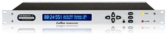
Meridian II Precision TimeBase.
The Meridian II Precision TimeBase references GPS to provide ultra-accurate time (10 nanoseconds to UTC) and frequency. At the core of Meridian II is a new GPS receiver that EndRun optimized to deliver a variety of traditional- and network-based time and frequency signals.
“The second-generation Meridian II continues EndRun’s heritage of pushing the envelope by delivering an industry-best, UTC time accuracy of 10 nanoseconds.” said Ron Holm, marketing manager, EndRun Technologies. “Meridian II also introduces a security-hardened, high-bandwidth network interface to synchronize evolving, network-centric applications via the Network Time Protocol (NTP) and IEEE-1588 Precision Time Protocol (PTP). Frequency standard customers will be happy to know that the revolutionary ultra-low phase noise and short-term stability performance of the original Meridian continues to be provided.”
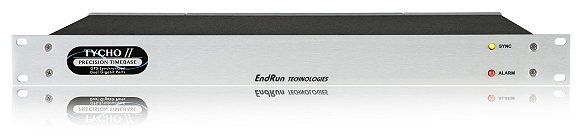
Tycho II Precision TimeBase.
Also new is the Tycho II Precision TimeBase time and frequency standard, which references GPS to provide exceptional time (25 nanoseconds to UTC) and frequency (<1×10-13 per day) accuracy in a security-hardened, network-centric platform.
At the core of Tycho II is a new EndRun GPS receiver that is optimized to take advantage of improved GPS system accuracy. Tycho II delivers a variety of traditional and network-based time and frequency signals and services via a modular, customer-configurable platform. Operational status is easily monitored via the network interface (HTTPS, SNMP, SSH). Intuitive charts are provided to assess current and historical performance of Tycho II, its GPS receiver and reference oscillator.
“The second-generation Tycho II provides our customers with a cost-effective, high-performance time and frequency standard without compromise to security and reliability,” said Dan Paine, sales and support manager, EndRun Technologies. “In addition, Tycho II uses the same network-centric core of our ultra-high performance Meridian II TimeBase. This enables operation as a high-bandwidth, Network Time Protocol (NTP) server and optional IEEE-1588 Precision Time Protocol (PTP) Grandmaster.”
Both the Meridian II and Tycho II have modular architecture that allows customers to configure them to meet specific application requirements.
The units support mission-critical operations in a wide range of government and commercial applications including telecommunications, satellite communications, digital video broadcast, simulcast radio, test range, test and measurement, calibration labs and power utilities.
Part 1 of this column appeared in the June Survey Scene newsletter, Part 2 appeared in the August newsletter. Upcoming Survey Scene newsletters will carry additional columns in this series.
Basic Understanding of Scientific and Hybrid Geoid Models
David B. Zilkoski
In my first newsletter column of this series, I discussed the basic concepts of GNSS-derived heights. I discussed the three types of heights involved in determining GNSS-derived orthometric heights: ellipsoid, geoid and orthometric.
In my second column (Part 2), I discussed guidelines for detecting, reducing, and/or eliminating error sources in ellipsoid heights. The column focused on guidelines for establishing accurate ellipsoid heights in a local geodetic network.
This column, Part 3, will describe the differences between a scientific gravimetric geoid model and a hybrid geoid model, and why it is important to use both geoid models in your analysis. The latest published United States National Geodetic Survey (NGS) hybrid geoid model, Geoid12B, is made consistent with the United States National vertical height reference frame, that is the North American Vertical Datum of 1988 (NAVD 88). This means a user will be consistent with NAVD 88 when using GEOID12B to estimate GNSS-derived orthometric heights. However, this doesn’t guarantee that your GNSS-derived orthometric heights are accurate.
NGS’ new Beta experimental geoid height models xGEOID14B and xGEOID15B are not distorted to fit the published NAVD 88 heights so they are useful for identifying valid NAVD 88 bench marks (that is, ensuring the monuments haven’t moved since their last survey and their published heights are still valid). Therefore, it is extremely important to validate all NAVD 88 height constraints used to estimate accurate GNSS-derived orthometric heights. Understanding NGS’ scientific and hybrid geoid models will help the user perform the appropriate analysis to determine which leveling-derived orthometric height constraints should be used as constraints. This newsletter will focus on differences between geoid models in a local project area.
Information on NGS’ experimental geoid models can be found here.
Thursday, August 20, 2015
Yearly Experimental Geoid Model Available for Public Review
In 2022, NGS will replace the current North American Vertical Datum of 1988 with one that is based on the geoid — a model of global mean sea level that is used to measure precise surface elevations. NGS created and released annual experimental models of the geoid starting in 2014. This year’s models, xGEOID15A and xGeoid15, are now available for public comment on the NGS beta website. The annual experimental models include new data from the Gravity for the Redefinition of the American Vertical Datum project, which has systematically collected airborne gravity data across the nation since 2008. For more information, contact: [email protected]
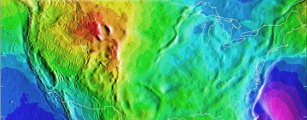
A depiction of the United States geoid. Areas in yellow and orange have a slightly stronger gravity field as a result of the Rocky Mountains.
While we often think of the earth as a sphere, our planet is actually very bumpy and irregular.
The radius at the equator is larger than at the poles due to the long-term effects of the earth’s rotation. And, at a smaller scale, there is topography—mountains have more mass than a valley and thus the pull of gravity is regionally stronger near mountains.
All of these large and small variations to the size, shape, and mass distribution of the earth cause slight variations in the acceleration of gravity (or the “strength” of gravity’s pull). These variations determine the shape of the planet’s liquid environment.
If one were to remove the tides and currents from the ocean, it would settle onto a smoothly undulating shape (rising where gravity is high, sinking where gravity is low).
This irregular shape is called “the geoid,” a surface which defines zero elevation. Using complex math and gravity readings on land, surveyors extend this imaginary line through the continents. This model is used to measure surface elevations with a high degree of accuracy.
How Does the U.S. National Geodetic Survey Generate a Geoid Model?
Generating geoid models is a fairly complex process and is performed by individuals with expertise in physical geodesy and geophysics. It is too complex of a topic for this newsletter but the following excerpt from an NGS publication by Dan Roman provides a good overview of NGS’ process.
Development of the North American Gravimetric Geoid: Adapting the Process to Determine a Unified Central American Geoid
D.R. Roman National Geodetic Survey, 1315 East-West Highway, Silver Spring, MD, USA, 20910
2 Data & Process Improvements
Techniques discussed here have already been addressed previously in Roman and Smith (2001) and Smith et al. (2001), hence only a summary of the approach discussed in those papers is given here. Essentially, the approach currently under investigations seeks to take advantage of recent and pending gains in various data sets related to the gravity field and significantly reduce approximations considered acceptable in the past.
The first thing to consider is the justification for using a geoid over a quasi-geoid, or more accurately, orthometric heights over normal heights. Convincing arguments have been made for orthometric heights (Holdahl 1984) and normal heights (Heiskanen and Moritz 1967). While orthometric heights require extensive knowledge of the gravity field, it is just that reason that warrants their use. Given the extensive knowledge and available data sets, it is incumbent on governmental agencies to generate such models. With a model of the gravity field from the surface to the geoid at hand, anyone subsequently desiring to transform from orthometric to normal heights need only apply it. However, if normal heights are developed and orthometric heights are later desired, the development of such a model will then be required. Clearly, this is a task best suited to national and international organizations that have access to such data and methods. It should not be left to those researchers desiring to use height models in their studies that may not have access to sufficient resources to accomplish this.
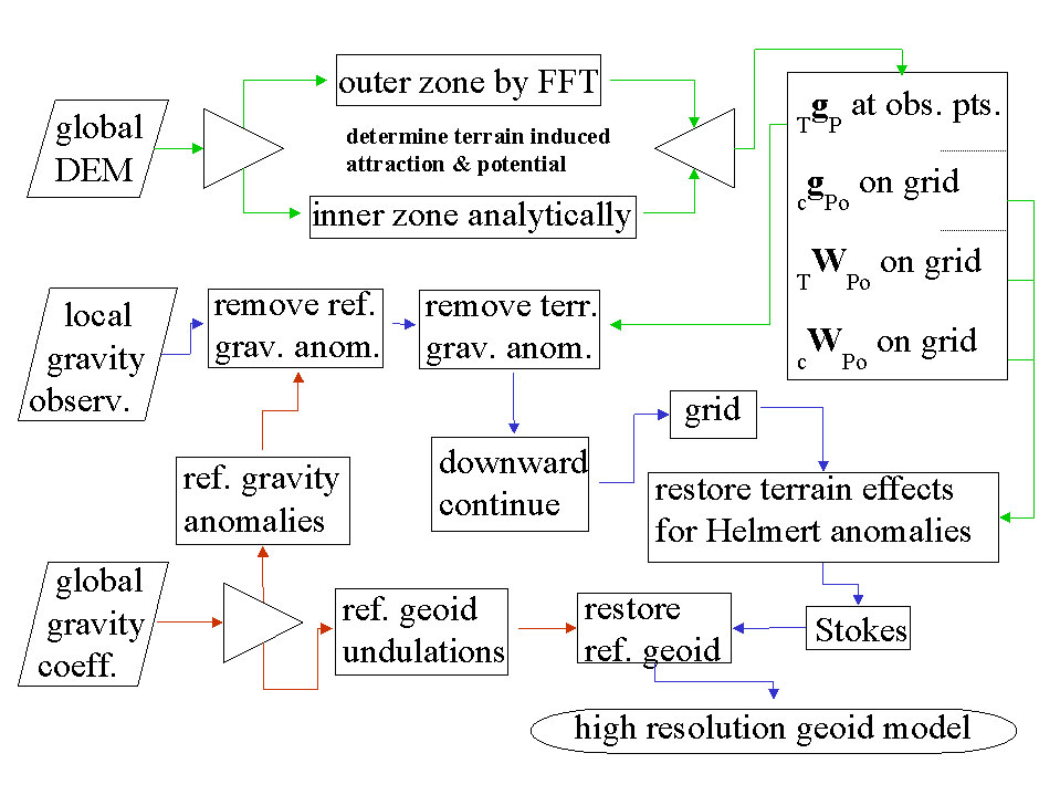
With that understanding then, the development of a gravimetric geoid model follows as a mechanism to readily convert between ellipsoidal and orthometric heights. The method summarized here seeks to break the gravity field into three components and solve them separately. In fact the long wavelength component will be derived from a global reference gravity model. The short wavelength will be determined from the terrain. Both of these components will be removed from available gravity observations, which will then reflect the intermediate wavelength signal. A flowchart depicting the determination of these three signals and the generation of a gravimetric geoid is given in Figure 1. Paths shown in red highlight the use of the reference model, paths in green show the determination of the terrain effects, while paths shown in purple highlight the main path to determining Helmert anomalies and then a gravimetric geoid model.
Fig. 1 Determination of a gravimetric geoid using Helmert anomalies.
The expected accuracy of global gravity models in the near future is expected to vastly improve with commission errors below 1-2 cm at wavelengths of 200-300 km (Tscherning et al. 2000). Use of a remove and restore technique (Bašiæ and Rapp 1992) will then result in significantly reduced errors in the residual signal that will be manipulated.
The approach discussed in Roman and Smith (2001) develops the North American gravimetric geoid by removing the terrain effects, downward continuing the residual values, and then restoring the effects of the condensed terrain to generate Helmert anomalies (Heiskanen and Moritz 1967).
To this end, the gravitational attraction of the terrain (TgP) will be calculated and removed from the gravity observations. It will be split into inner and outer zones to reduce computation times. Smith et al. (2001) showed that the effects of using FFT to determine gravitational attraction and potential for both condensed and 3D masses is negligible beyond about a 4 degree cap radius from the point of interest (P). Inside that zone, DEM’s are employed to capture the spherical relationships between the points and more accurately determine the attraction. With available or pending 1 and 3 arc-second DEM’s (Smith and Roman 2001a, NIMA 2001), the signal that may be determined is limited mainly by the computational facilities available to a researcher.
Additionally, the DEM’s will be used to construct grids for the attraction and potential of the condensed terrain (cgPo and cWPo), as well as the potential of the actual terrain (TWPo), all on the geoid. This will capture the short wavelength gravity signal represented by the terrain to the resolution of the grid generated and facilitate later incorporation of this signal into Helmert anomalies.
The resulting point values should be composed mainly of intermediate features in the gravity field with sources deriving from variations in the Moho depth and lateral density variations. This signal should be sufficiently smooth to reduce errors resulting from downward continuation. It should also sufficiently sample the intermediate field to permit the use of minimum curvature (Smith and Wessel 1990) to generate a grid at the same interval as that of the above terrain effects.
Once these terrain effects are restored, these extremely high resolution grids represent residual Helmert anomalies and may be processed using the Stokes integral to determine a best fitting residual gravimetric geoid. Adding the reference geoid derived from the selected global coefficient model will create an equally high-resolution regional gravimetric geoid model.
For a specific country, GPS-derived ellipsoid heights at leveled bench marks (GPSBM’s) provide control information for generating a hybrid geoid model that can be used to specifically, easily, and accurately transform heights between ellipsoidal and orthometric heights (Smith and Milbert 1999, Smith and Roman 2001b).
What are Hybrid Geoid Models and how are they Generated?
NGS’ hybrid geoid model GEOID12B is computed based on the gravimetric geoid USGG2012. As described above, the gravimetric geoid is computed using the satellite model (GOCO3S), terrestrial gravity data, and the altimetric gravity anomaly over oceans. The heights of USGG2012 represent an equipotential surface relative to the reference ellipsoid. The differences between USGG2012 and the zero height surface of NAVD88 are represented by NAD 83 (2011) GNSS-derived ellipsoid heights on NAVD 88 published benchmarks (GPSBM data). See article by Milbert, D.G., 1998: “Documentation for the GPS Benchmark Data Set of 23-July-98,” IGeS Bulletin N. 8, International Geoid Service, Milan, pp. 29-42.) for a excellent description of NGS’ GPSBM dataset.
Currently, the USGG2012 is fitted to the GPSBM data by using the method of least squares collocation. (See section labeled “Excerpts from NGS’ Geoid 12 Web Page” for specific details on how NGS generated hybrid geoid model GEOID12B.) Areas where there are no GNSS observations on published NAVD 88 benchmarks are filled in by USGG2012 geoid. This means a user will be consistent with NAVD 88 when using GEOID12B to estimate GNSS-derived orthometric heights. Being consistent with NAVD 88 is important but being consistent doesn’t guarantee that your GNSS-derived orthometric heights are accurate. The documentation of GEOID12B states that “The relative accuracy of GEOID12B to NAVD88 is characterized by a misfit of +/-1.7 centimeters nationwide.” However, if a published NAVD 88 height used in the development of the hybrid geoid model isn’t valid, then the model is precise but not accurate. That’s why it is important to ensure the monuments used in hybrid geoid models haven’t moved since their last survey and that their published heights are still valid. We will discuss this in more detail later in this newsletter.
Hybrid geoid model, GEOID12B is computed based on the gravimetric geoid USGG2012 . More specifically, they are computed using the satellite model GOCO3S, terrestrial gravity data, and the altimetric gravity anomaly over oceans. The heights of USGG2012 represent an equipotential surface relative to the reference ellipsoid. The differences between USGG2012 and the zero height surface of NAVD88 are represented by GPSBM data.
Currently, the USGG2012 is fitted to the GPSBM data by using the method of least squares collocation. That implies that the voids or empty areas where there are no GPSBM data are filled in by USGG2012 geoid.
There are over 500,000 leveled marks and 80,000 GPS marks over U.S. territory. Of those, there are only 26,000 GPSBM, with half of them concentrated in 5 states. The data density is uneven and sparse in some states. Lists of GPSBMs can be downloaded from the GEOID12B home page.
The GPSBM data provide the geoid height ‘N’ by differencing the ellipsoidal height ‘h’ from the orthometric height ‘H’:
N = h – H
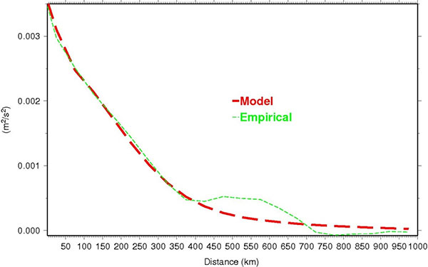
The difference between the geoid height N and that of USGG2012 is computed at every GPSBM. Then, a mathematical model using Least Squares Collocation (LSC) fitting Gaussian functions to describe the behavior seen at the GPSBM is developed. Figure 1 shows empirical data versus the model.
Figure 1: Covariance functions of the geoid differences between USGG2012 and GPSBMs.
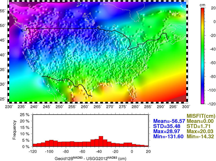
Once the relationship between the points is modeled, the model is used to generate a regular grid for interpolation purposes. Figure 2 shows the final conversion surface. This surface represents the difference between NAVD 88 as a datum and the geopotential (geoid) surface used in the gravimetric geoid and is representative of what the datum transformation surface will be when the new geopotential datum is released in 2022. (Similar to VERTCON, which transforms heights from NGVD29 to NAVD88.)
Figure 2: GEOID12B conversion surface.
Summary and Recommendations
Three hybrid geoid models GEOID12, GEOID12A, and GEOID12B are created. They are very similar, but have distinctive differences in few areas. GEOID12A differs from GEOID12 in that it does not use GPSBM data collected in the southern tier states along Gulf Coast, while GEOID12B differs from GEOID12A only in Puerto Rico.
Data in the database are constantly updated, hence older geoid models do not reflect the newer data. To guarantee data consistency, latest model should be used. At this time, GEOID12 and GEOID12A should be superseded by GEOID12B.
Use data conversion outside the GPSBM data areas with caution. Significant extrapolation errors are expected in areas where there are no GPSBM data.
The relative accuracy of GEOID12B to NAVD88 is characterized by a misfit of +/-1.7 centimeters nationwide.
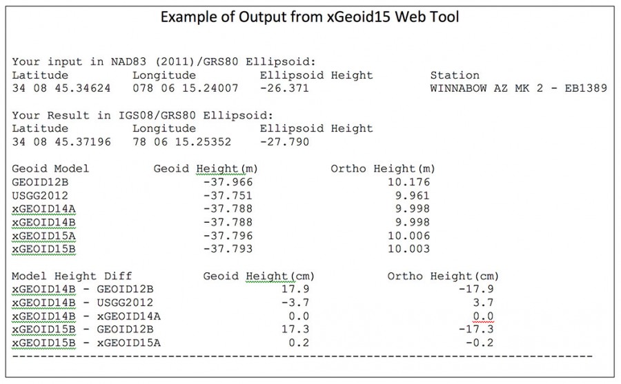
As previously stated, NGS released its latest gravimetric geoid model, xGEOID15. This site will allow the user to compare geoid heights from GEOID12B, USGG2012, xGEOID14 and xGEOID15. (See an example of an input and an output file below.) There are some limited features to this tool. It only provides the results in IGS08 and you are limited to the number of coordinates you can submit at once (20 stations).
Saying that, this tool can be useful for identifying valid NAVD 88 published monuments to be used in the development of future hybrid models. More importantly, it can be used to identify monuments that should NOT be used in future hybrid geoid models or used as constraints in GNSS survey project adjustments.
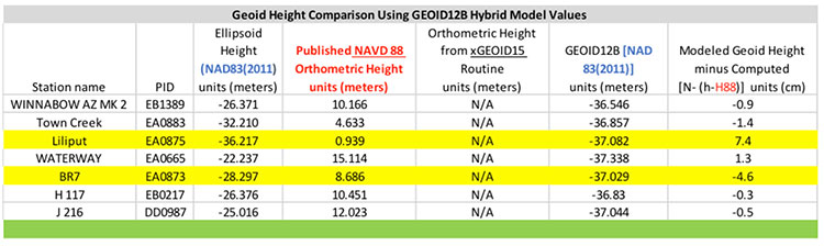
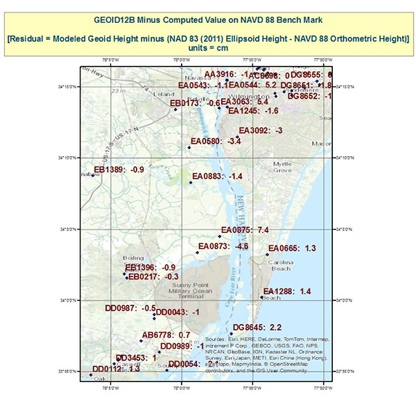
First, let’s look at the hybrid geoid model GEOID12B values compared with computed geoid height values using the equation N (Computed Geoid Height) = [h (NAD 83 (2011) Ellipsoid Height) – H (NAVD 88 Orthometric Height)]. Table 1 lists the differences between the modeled GEOID12B values and the computed geoid height values for a few stations in an area in eastern North Carolina. Figure 1 depicts the stations locations and values. Many of the differences are less than 1.5 cm which is consistent with NGS’ documentation of GEOID12B that states “The relative accuracy of GEOID12B to NAVD88 is characterized by a misfit of +/-1.7 centimeters nationwide.” However, what is important to notice is that two stations have large differences; station LILIPUT’s difference is 7.4 cm and station BR 7’s difference is -4.6 cm (See highlighted rows in table 1 and boxed area on figure 1). This means that the relative difference between stations LILIPUT (EA0875) and BR 7 (EA0873), which are only 3.3 km apart, is 12.0 cm. This is a large difference and may be indicating a large error in the ellipsoid height and/or the orthometric height at station LILIPUT (EA0875) or station BR 7 (EA0873). In the second newsletter we highlighted that stations LILIPUT and BR 7 were only 3.3 km apart but were not simultaneously observed during the same session. Since the relative difference is 12 cm, the ellipsoid heights of these two should be investigated. It should also be noted that the difference between stations BR 7 (EA0873) and TOWN CREEK (EA0883) is only 3.2 cm. This implies that station B 7 (EA0873) is consistent with some of its neighbors. In the second newsletter we noted that stations B 7 (EA0873) and TOWN CREEK (EA0883) were simultaneously observed during the same session. This may be an indication that B 7 is stable relative to its neighbors and that the orthometric and/or the ellipsoid height of station LILIPUT needs to be investigated.
So what does this mean to the user? If the user establishes a GNSS-derived orthometric height near station LILIPUT using GEOID12B, their results will disagree with the published NAVD 88 heights to around 7 cm; if they establish a GNSS-derived orthometric height near station BR 7, they will disagree with published NAVD 88 heights to around –5 cm. This could also mean that the results in a project could really disagree by more than 7 cm if station LILIPUT moved since its last survey. At this moment, we don’t have enough information to determine if the ellipsoid height or the orthometric height is the problem, or which station may have moved since its last survey.
Table 1. Geoid Height Comparison using GEOID12B Hybrid Model Values.Figure 1. Geoid12B minus Computed Value on NAVD 88 Benchmarks.
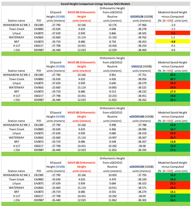
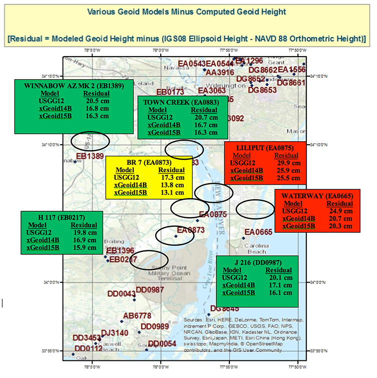
Next, let’s look at the differences using the experimental geoid models which are not distorted to be consistent with the NAVD 88 published heights. There will be a bias and a tilt between the systems but in this small areal extent the tilt should not be significant to our analysis. The bias can be removed by looking at relative differences between stations. Table 2, titled “Geoid Height Values for Various NGS Models using xGeoid15 Web Tool,” provides the modeled geoid height minus the computed geoid height where N (Computed Geoid Height) = [h (IGS08 Ellipsoid Height) – H (NAVD 88 Orthometric Height)]. Figure 2, titled “Various Geoid Models minus Computed Geoid Height,” depicts the differences between the various experimental models and computed geoid heights.
Table 2. Geoid Height Values for Various NGS Models using xGeoid15 Web Tool.Figure 2. Various Geoid Models minus Computed Geoid Height.
What is important to note is that stations LILIPUT (EA0875) and WATERWAY (EA0665) seem to be outliers compared to the other stations in the area of study (red boxes on figure 2); and station B 7 (EA0873) seems to be consistent with its neighbors (yellow box on figure 2). For example, station LILIPUT (EA0875)’s residual using xGeoid15B is 25.5 cm and station BR 7 (EA0873)’s residual using xGeoid15B is 13.1 cm, a relative difference of 12.4 cm. Similarly, station TOWN CREEK (EA0883)’s residual using xGeoid15B is 16.3 cm and station BR 7’s residual is 13.1 cm, a relative difference of only 3.2 cm. In my opinion, station LILIPUT (EA0875) needs to be investigated to determine if it has moved since it was last surveyed. In addition, stations east of LILIPUT (EA0875) such as WATERWAY (EA0665) should also be investigated for an ellipsoid and/or orthometric height issue. As previously mentioned, it is also important to note that station BR7 (EA0873), the box in yellow, appears to be consistent to the 3 cm level with its westerly neighboring stations (the boxes in green). This is important to note because the hybrid geoid model could be significantly difference around stations LILIPUT and BR 7 if station LILIPUT was not used in the development of the hybrid geoid model. I am not suggesting that NGS did anything incorrect by including these stations. The goal of the hybrid geoid model is to be consistent with published NAVD 88 values. Unless there is enough information to determine that a station has moved since the last time it was surveyed, the station should be included in the hybrid model. This is where the user may be able to help NGS. If users would investigate outliers like LILIPUT and BR 7 and provide new GNSS survey data and/or leveling data, NGS may have the appropriate information to determine if the monument should be included in the hybrid model.
Part 2 in this Survey Scene series discussed procedures which need to be followed to detect, reduce, and/or eliminate error sources to estimate accurate GNSS-derived ellipsoid heights. This column, Part 3, discussed why a user should understand the differences between NGS’ scientific gravimetric geoid model and hybrid geoid models, and why it is important to use both types of geoid models in their analysis. It demonstrated how to use these geoid models and ellipsoid heights to identify potential issues with published NAVD 88 heights.
My next newsletter column will focus on analyzing the NAVD88 orthometric heights in this area. It will provide basic procedures for validating NAVD 88 height constraints used to estimate GNSS-derived orthometric heights.
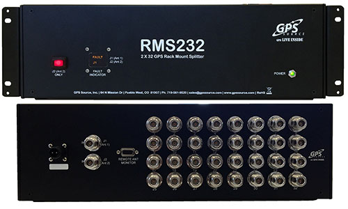
GPS Source has released a GPS/GNSS rackmount splitter with dual antenna inputs and antenna health monitoring. Developed for the wireless industry, the dual-input splitter provides a GPS timing signal to up to 32 GPS/GNSS synchronization modules and receivers. Its design ensures the GPS timing signal is always available, even in the event of an antenna or cable failure, the company said.
Like GPS Source’s GPS rackmount splitters, the new rackmount splitter amplifies and splits the GPS/GNSS signal. However, the new splitter also includes dual GPS antenna input ports, a health monitor and sensor switch. Up to 32 GPS/GNSS receivers or timing synchronization modules can access the signal at one time. Antenna redundancy is acquired through the use of primary and backup antennas. The sensor monitors the health of the primary antenna connected to the splitter. Based on the information provided by the sensor, the splitter will automatically switch antennas. The ability of the splitter to switch antennas allows all connected GPS devices to remain fully functional in the event of an antenna failure, which is important in today’s wireless environment.
“The demand for high-speed wireless internet and data network access over a wide area has grown at a record pace,” said Robert Horton, CEO of GPS Source. “This growth has led to a strong demand for solutions that support more than one function because of limited space and increased usage. The new rackmount splitters, RMS216 and RMS232, will keep multiple timing synchronization modules operating for an extended period when a GPS antenna or cable fails. This extended period gives a solution provider supporting a cell site, base station, or DAS network, the ability to identify and fix any GPS/GNSS antenna or cable problem before other challenges arise.”
The U.S. Department of Transportation’s Federal Aviation Administration (FAA) has announced the largest civil penalty the FAA has proposed against a UAS operator for endangering the safety of the national airspace.
The FAA proposes a $1.9 million civil penalty against SkyPan International Inc. of Chicago. Between March 21, 2012, and Dec. 15, 2014, SkyPan conducted 65 unauthorized operations in some of the most congested airspace and heavily populated cities, violating airspace regulations and various operating rules, the FAA alleges. These operations were illegal and not without risk.
The FAA alleges that the company conducted 65 unauthorized commercial UAS flights over various locations in New York City and Chicago for aerial photography. Of those, 43 flew in the highly restricted New York Class B airspace.
“Flying unmanned aircraft in violation of the Federal Aviation Regulations is illegal and can be dangerous,” said FAA Administrator Michael Huerta. “We have the safest airspace in the world, and everyone who uses it must understand and observe our comprehensive set of rules and regulations.”
SkyPan operated the 43 flights in the New York Class B airspace without receiving an air traffic control clearance to access it, the FAA alleges. Additionally, the agency alleges the aircraft was not equipped with a two-way radio, transponder and altitude-reporting equipment.
The FAA further alleges that on all 65 flights, the aircraft lacked an airworthiness certificate and effective registration, and SkyPan did not have a Certificate of Waiver or Authorization for the operations.
SkyPan operated the aircraft in a careless or reckless manner so as to endanger lives or property, the FAA alleges.
SkyPan has 30 days after receiving the FAA’s enforcement letter to respond to the agency.
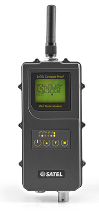
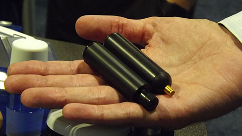
Satel’s new UHF radio data modem Compact-Proof, designed for outdoor measurement applications, features autonomous rechargeable battery power and a robust housing with IP67 protection.
Compact-Proof from Satel gives users double advantages with a powerful lithium-ion battery and the EASy radio data technology including a display and a robust housing with IP67 protection, the company said. With transmitting power of 1,000 mW, it can be operated fully autonomously as a repeater station in the field for more than 15 hours. The power can also be supplied parallel via an external rechargeable battery with a solar panel; alternatively, the Compact-Proof can be recharged overnight, and within five hours it is ready for the next work day.
The user-friendly installation, robust IP67 housing and 4-pin and 8-pin ODU connections make the new radio data modem Compact-Proof attractive for measurement applications, Satel said. The device features all functions of the Satel radio data modems EASy and 3AS and is 100 percent compatible with these solutions.
In addition, it supports the radio protocols of Pacific Crest, Trimble and other GNSS providers, which expands the areas of application.
Whether in the rainforests of Vietnam or in the Arctic, the temperature range of -30°C to +65°C and the frequency ranges of 330 MHz…420 MHz and 403 MHz…473 MHz make the Compact-Proof a reliable partner for all outdoor applications, Satel said. The housing features a robust, compact design with a display and foil keyboard.
As a light version — without an internal battery — the device offers numerous advantages for outdoor applications and even withstands the harsh conditions of machine control environments, for example.
In Germany, radio data transmission solutions from Satel are distributed exclusively by systems provider Welotec.
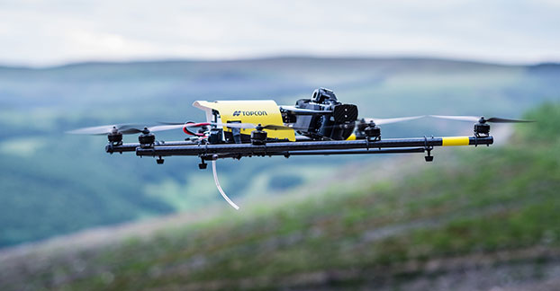
Topcon Positioning Group has added a rotary-wing unmanned aerial system (UAS) to its mass data-collection solutions line. The Falcon 8 — powered by Ascending Technologies — is designed for inspection and monitoring, as well as survey and mapping applications.
“Rotary-wing systems provide the perfect solutions for small-scale sites and projects for which flexibility of takeoff and landing or an oblique perspective is required,” said Charles Rihner, vice president of the Topcon GeoPositioning Solutions Group. “The Falcon 8 offers the flexibility to maneuver in small spaces and can cope with challenging environments often presented in inspection and monitoring. It is also well suited for smaller mapping or modeling projects up to 85 acres that require high-resolution imaging.”
The Falcon 8 features new AscTec Trinity technology, an autopilot safety feature that provides three levels of redundancy for protection against performance drop or loss of control. Three IMUs (inertial measurement system) synchronize all sensing data and identify, signal and compensate when needed.
Two models are available — the GeoEXPERT for surveying, modeling and mapping projects, and InspectionPRO for industrial inspection and monitoring applications. The GeoEXPERT includes a HD RGB camera payload, while the InspectionPRO features an HD RGB camera and infrared sensor combination.
“Both versions offer easy deployment and operation with real-time video and data monitoring capability, navigation software for planning and optimizing flights, as well as photo-tagging and desktop software to quickly generate high-quality and easy-to-edit material,” said Rihner.
The Falcon 8 complements the Topcon Sirius Pro fixed-wing UAS, providing large area accurate mapping without the requirement for traditional ground control.
Wide-Area Wireless Network Synchronization with LocataNets
The United States Naval Observatory conducted several independent frequency synchronization experiments in Washington, D.C., using an alternative PNT technology in multiple network configurations. The results suggest that sub-nanosecond time transfer using this technology may be possible over wide urban areas, and that it could thus serve as a GPS augmentation or back-up solution over wide areas for critical applications that depend on precise time.
By Edward Powers and Arnold Colina
Because of the great responsibility of being the prime source of time for many critical national systems, the United States Naval Observatory’s (USNO’s) clock system must be at least one step ahead of the demands expected to be made on its accuracy. Therefore, innovative methods of transferring precise time and frequency must continually be anticipated, investigated and supported.
The USNO has developed one of the world’s most accurate and precise atomic clock systems, used by many systems requiring highly precise time. The USNO operates the U.S. Master Clock, which provides the precise time source for the GPS satellite constellation run by the Air Force; it is also the time standard for the U.S. Department of Defense. Along with its sister organization, the National Institute of Standards and Technology (NIST), it provides the official time for the entire nation.
To investigate new precise time transfer methods, the USNO desired to independently test Locata’s TimeLoc methodology as a possible technology for maintaining precise frequency synchronization across an urban or wide-area network — the foundation for supporting precise time transfer.
Internet of Everything Ups Timing Requirements
Many critical modern systems such as 4G mobile phone networks, banking, and electricity grids demand high-accuracy time and frequency stability across specified areas. Precise network synchronization is critical for nearly all digital networks, and more stringent network stability requirements are expected to emerge as the user base for these applications continues to grow. To date, the preferred method to achieve this performance is via synchronization from GPS. However, the vulnerability of GPS signals causes growing concern among industry experts. Many actively seek alternative means of precise time transfer and frequency stability across wide areas.
Alternative position, navigation, and timing (PNT) technologies such as chip scale atomic clocks (CSAC), precision time protocol (PTP), and enhanced long range radio navigation (eLoran) are proposed or operational today, with each serving different markets.
Meanwhile, timing needs for wireless protocols continue to increase with the proliferation of mobile phones and other wireless communication devices. To accommodate a booming user base, wireless spectrum must be carefully managed to improve bandwidth and channel efficiency. Wireless communication performance is fundamentally dependent upon precise time and frequency, so improvements in highly accurate timekeeping methods will permit better spectrum utilization, which in turn permits more users and more bandwidth per user.
Clearly, synchronization is a core enabling technology for modern digital systems, both for radiopositioning and the world’s telecommunications highways. But synchronization is taken for granted because, when it works well, it is effectively invisible. Without it, however, everything is likely to fall apart.
Synchronization will become even more crucial for the next generation of digital systems. A recent paper by the U.S. National Institute of Standards and Technology (NIST) states that we stand at the advent of a revolutionary new economy fueled by a global Internet of Everything (IoE), in which 37 billion new things will be connected to the Internet by 2020.
This NIST paper adds that “One fundamental enabler of this revolution will be the marriage of timing signals and data that breaks through the existing barriers. Timing is critical for future development and improvements.”
Improved wireless synchronization has proved very challenging to realize, as the timer in each network node is derived from an independent oscillator that is affected by long/short term frequency drifts and jitter. Many alternative timekeeping methods present serious limitations in terms of precision or network size.
Encouraged by earlier published results showing that Locata Corporation’s radio-based PNT technology enables network synchronization at the nanosecond level, and suggesting that it could perform comparably across large urban areas, the United States Naval Observatory (USNO) conducted its own synchronization experiments on Locata technology.
Real-World Challenges
The USNO campus is situated about 4 kilometers northwest of the White House in Washington, D.C. The grassy tree-lined campus is, unfortunately, a relatively small area for testing wide-area synchronization capabilities. It became apparent that realistic long-distance tests would necessitate extending the LocataNet outside USNO boundaries. This meant coordinating access to other facilities in theWashington, D.C., area to allow remote housing of LocataLites and their antennas. As many researchers will confirm: when real-world testing requires access to multiple external sites and their disparate administrations, the coordination required to keep everything on track can quickly become the most daunting challenge of the exercise. We needed to find cooperative facilities, preferably with line-of-sight (LOS) to the USNO and its Master Clock in order to establish the best TimeLoc link between facilities. As we also wanted to exercise TimeLoc’s ability to cascade its synchronization through multiple LocataLites, ever more D.C. facilities would need to be involved. Predictably, it transpired that not many facility managers in the Washington district were eager to help the USNO broadcast and receive new and unknown signals in or around their government buildings! And those who were amenable to support the demonstration either lacked a LOS, or were not willing to assist without considerable monetary compensation.
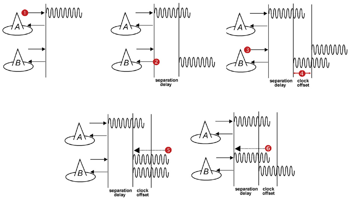
Step 1: LocataLite A transmits a unique signal (code and carrier). Step 2: LocataLite B acquires, tracks and measures the signal generated by A. Step 3: LocataLite B generates its own unique signal (code and carrier) which is transmitted in the normal manner. Importantly, the transmitted signal is received by the receiver section of LocataLite B as well. Step 4: LocataLite B calculates the difference between the signal received from LocataLite A and its own locally generated and received unique signal. Ignoring propagation errors, the differences between the two signals are due to the difference in the clocks between the two devices, and the geometric separation between them. Step 5: LocataLite B adjusts its local oscillator to bring the differences between its own signal and LocataLite A’s received signal to zero. The signal differences are continually monitored and adjusted so that they remain zero. In other words, the local oscillator of B follows precisely that of A. Step 6: The system corrects for the geometrical offset (range) between LocataLite A and B, using the known coordinates of the LocataLites’ antennas. When this step is accomplished, TimeLoc has been achieved.
After months of attempts to secure appropriate partners for this demonstration, we finally found some supporters in the shape of the Federal Aviation Administration Building in Rosslyn, Va., and the National Cathedral in Washington, D.C. Regrettably, it turned out that these facilities were not going to be available at the same time! Logistic challenges never end. This scheduling reality necessitated spreading the TimeLoc demonstration over several months in three different blocks of trials. Nevertheless, we were eventually able to devise a plan which leveraged access to the USNO and still accommodated the timetables of the supporting external facilities.
A series of experiments were planned to measure and evaluate the stability between master and slave LocataLite 1-pulse per second (PPS) signals in several urban LocataNet configurations. Many of the trials were specifically designed to measure TimeLoc’s ability to cascade multiple times through multiple LocataLites, exercising the technology’s capabilities over increasing distances and hence correspondingly larger notional coverage areas.
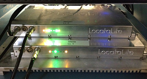
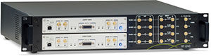
Figure 2. LocataLites under test at USNO.
Locata signals were broadcast in the Industrial, Scientific and Medical (ISM) 2.4 GHz radio band, commonly known as the Wi-Fi band, with a total radiated power of 200–500 mW. LocataLites and their respective antennas were installed at locations that permitted LOS between units, according to whichever specific LocataNet configuration was being evaluated at the time. In each configuration, the master LocataLite, designated as LocataLite 1, was synchronized to the USNO Master Clock so that the Master Clock’s time would be propagated through the LocataNet. Both the master and slave LocataLite 1PPS signals were collected into a time interval counter and the time difference between their rising edges was measured.
When tracking radio frequency signals over a significant distance, tropospheric delay becomes an important error source for measurements used in timing solutions. The speed of light can only be assumed to be universally constant in a vacuum, so atmospheric temperature, pressure and humidity materially changes the speed of light when propagating through air. In fact, using standard atmospheric parameters, the unmodeled tropospheric delay is surprisingly large — approximately 280 parts per million (ppm), which equates to slowing down almost one nanosecond over each kilometer of radio transmission. Obviously, as transmission distances increase, tropospheric error becomes a substantial factor which must be accounted for in hyper-accurate timing systems. Devising methodologies that effectively mitigate large tropospheric errors becomes essential.
To help solve this problem, Locata developed new tropospheric models that use relatively inexpensive meteorological (MET) stations which measure temperature, pressure and relative humidity at the LocataLite sites. This modeling alone is able to mitigate the tropospheric effects to within just few parts per million. This proved to be an essential feature, as the weather during the course of the entire months-long testing campaign varied significantly among the separate trials.
The TimeLoc Process
LocataNets function as local ground-based replicas of the satellite-based GPS position and timing networks. A LocataNet can be designed and configured by the user to deliver a powerful, local, controllable, tailored signal as required by different applications.
The easiest LocataNet layout to describe is a hub-and-spoke model consisting of a single master LocataLite transceiver and one or more slave LocataLites. More complex network configurations have been deployed in many commercial systems in use today. The patented process by which slaves are synchronized to the master (or other slaves) is known as TimeLoc.
In 2013, a University of New South Wales team demonstrated that Locata’s radio-based TimeLoc technology provided accurate time transfer (~5 ns) and frequency stability (~1 ppb) across a large distance of 73 kilometers (45.4 miles). This significantly outperforms GPS for wireless time transfer. Given this demonstrated radius of transmission in a rudimentary configuration, Locata was shown as being able to supply nanosecond-accurate time to a 146 km diameter circle, which would cover 16,750 km2 — almost 200 times the size of Manhattan. Ranges greater than this can be deployed if required for safety-of-life, military or government-mandated systems.
As TimeLoc is accomplished without the use of atomic clocks, this represents a new level in precision network synchronization of this scale. It could conceivably serve as a GPS augmentation or back-up solution over wide areas for critical applications that depend on precise time.
Since Locata technology was originally developed as a high-accuracy non-GPS-based positioning and navigation solution, the time synchronization accuracy requirements for a LocataLite transceiver are very high. If sub-centimeter positioning precision is desired for a Locata receiver, every smallest fraction of a second is significant; for example, a 1-nanosecond error in time equates to an error of approximately 30 centimeters.
TimeLoc wireless synchronization enables LocataLites to achieve high levels of synchronization without atomic clocks, without external control cables, without differential corrections, and without a master reference receiver.
In theory, there is no limit to the number of LocataLites that can be synchronized together. TimeLoc allows a LocataNet to propagate into difficult environments or over wide areas. For example, if a third LocataLite C can only receive the signals from B (and not A) then it can use these signals from B for time synchronization instead. The only requirement for establishing a LocataNet using TimeLoc is that LocataLites must receive signals from one other LocataLite. This does not have to be the same central or master LocataLite, since this may not be possible in difficult environments with obstructions, or when propagating the LocataNet over wide areas.
This method of cascading TimeLoc through intermediate LocataLites has been proven in a growing number of real-world operational LocataNets, including a network in use today by the U.S. Air Force which is configured to cover up to 2,500 square miles (6,500 square kilometers) of the White Sands Missile Range in New Mexico.
In large networks where extremely high synchronization accuracies are required, it is useful to incorporate a meteorological sensor at each LocataLite to monitor the change in weather over considerable distances. This is certainly the case for long-range systems such as the USAF LocataNet installed at the huge White Sands Missile Range, where distances of over 50 km can be found between LocataLites. However, for the purposes of these USNO Washington experiments, where the longest point-to-point transmission distance was 2.9 km, it was assumed that weather parameters would be virtually identical at all LocataLite locations. Therefore only one MET station was employed within the entire network, which for these trials was collocated with the master LocataLite.
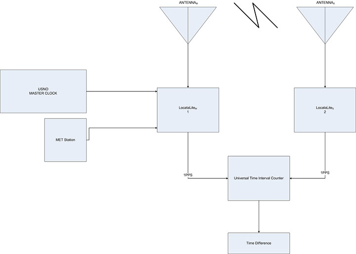
The very first experiment conducted by the USNO to gain some familiarization with TimeLoc was run entirely within the grounds of the USNO campus. It employed two LocataLites with their respective antennas on the roof of USNO Building 78. In this initial configuration the antennas were positioned 15.24 m apart. It was intended to use the measured result as a baseline against which TimeLoc synchronization over longer distance could be compared. This first arrangement is referred to as the two-node setup. A diagram of this configuration is shown in Figure 3.
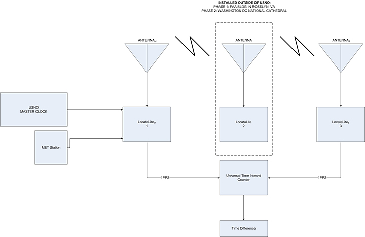
Second and third experiments demonstrated Locata’s ability to cascade the master 1PPS signal to an intermediary slave LocataLite, which in turn transmits a signal to which a third LocataLite can TimeLoc. This LocataNet configuration is referred to as the three-node setup (Figure 4).
Figure 4. Three-node setup (total range: 5.794 km/3.6 mi and 2.401 km/1.49 mi).
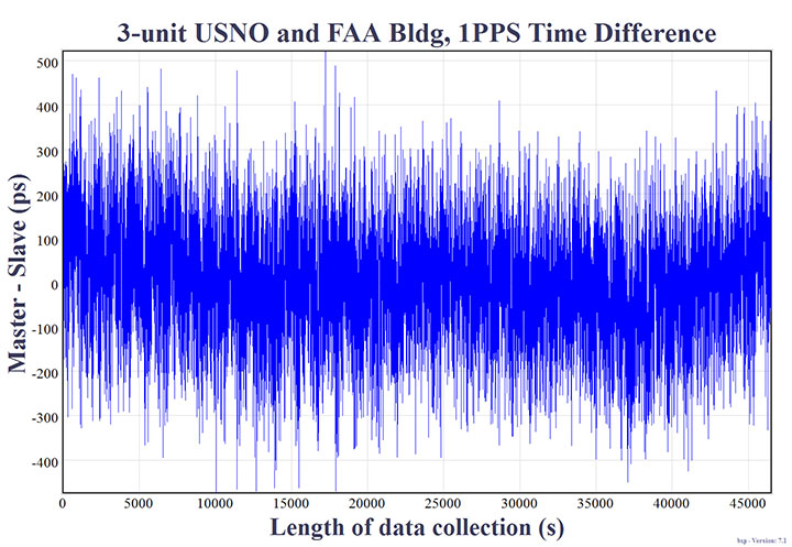
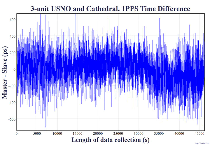
This experiment was conducted twice using two different intermediate LocataLite locations. The first intermediate location was indoors on the top floor of the FAA Building in Rosslyn, Va. (Figure 5). The distance between the master/slave antennas to the intermediate antenna in the FAA building was 2.897 km, but since the signal was propagated through a tinted window, the received signal strength inside the building was greatly attenuated, effectively simulating a much longer transmission distance. The second intermediate (LocataLite 2) location was from the balcony of the National Cathedral’s Ringing Chamber. In this case the distance between USNO LocataLite 1 master/slave to the intermediate antenna in the National Cathedral was approximately 1.183 km.
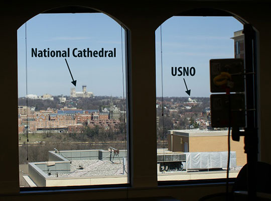
Figure 5. Intermediate LocataLite 2 antennas inside FAA building. In the distance, both the USNO and the National Cathedral are visible.
In both cases in Figure 4, the distance between master and terminal slave antennas was 3.048 m on the USNO building, but they were intentionally not TimeLoc’d to each other. The timing signal was therefore forced to route through the intermediate LocataLite 2 at either the FAA Building or the National Cathedral.
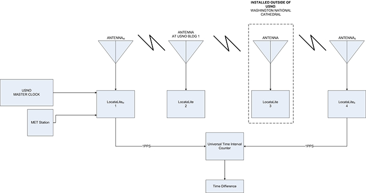
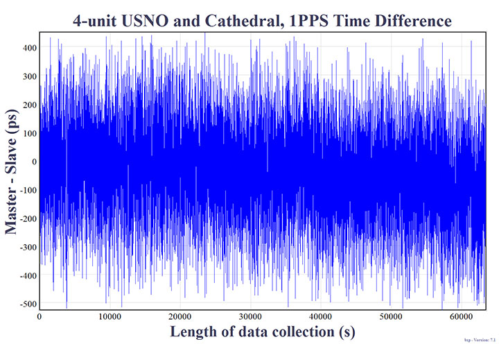
A fourth experiment included yet another intermediate cascade where the TimeLoc signal was transmitted from the second to a third LocataLite/antenna before arriving at the fourth LocataLite in the chain. This LocataNet configuration is referred to as the four-node setup. A diagram of the setup is shown in Figure 6, and it now added a LocataLite on USNO Building 1 to expand the set-up, along with the intermediate LocataLite installed at the National Cathedral (Figure 7).
Figure 6. Four-node setup (total range: 2.413 km/1.5 mi).Figure 7. LocataLite antennas outside the Ringing Chamber of the National Cathedral Spire.
Referring to Figure 6, the distance between the master LocataLite (antenna 1) at USNO Building 78 and the LocataLite (antenna 2) at USNO Building 1 was approximately 42.672 m. The distance between the USNO Building 1 (antenna 2) to the Washington National Cathedral (antenna 3), was approximately 1.144 km. The distance between the Washington National Cathedral (antenna 3) back to antenna 4 on USNO Building 78 was approximately 1.183 km. The total range in this four-node chain was 2.413 km. In this configuration, LocataLites 1 and 4 are intentionally not TimeLoc’d to each other, forcing the 1PPS signal to be routed through LocataLites 2 and 3.
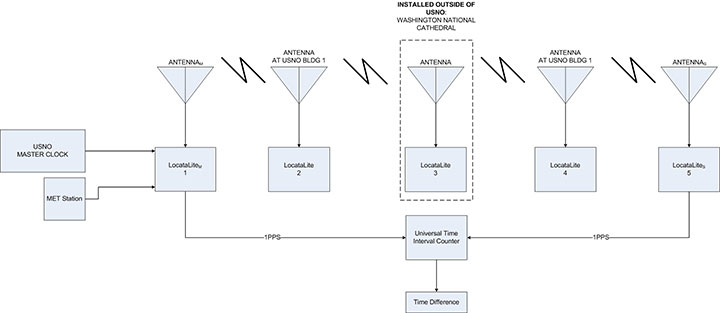
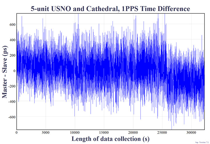
A fifth experiment included yet one more LocataLite and antenna at USNO Building 1 (Figure 9), totaling cascaded TimeLoc among five LocataLites and their respective antennas: the five-node setup, shown in Figure 8. In this configuration LocataLites 1 and 5 are intentionally not TimeLoc’d to each other, forcing the 1PPS signal to be routed through LocataLites 2, 3 and 4.
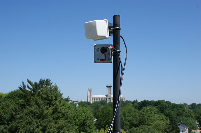
Figure 8. Five-node setup (total range: 2.427 km/1.51 mi).Figure 9. LocataLite antennas on USNO Building 1. National Cathedral in background.
Measurement Methodology
A measurement of time difference between master and slave LocataLite 1PPS readings was done using a Stanford SR620 universal time interval counter. The rising edge of the 1PPS signals were inspected at 1-Volt trigger level. A 10 MHz reference was provided to the counter from the USNO’s Master Clock. Channels A and B on the counter were designated to the master and slave 1PPS signals respectively. Data were collected from the counter through serial connection to a PC. The length of each experiment was time-limited in some way because of limited access to facilities, such as the FAA building or National Cathedral. However, a minimum of at least 30,000 seconds (8.33 hours) of data were collected for each test to characterize the overall stability of the 1PPS signals between master and terminal slave LocataLites.
Collected Data
Figures 10 to 14 show the normalized 1PPS time difference between the master LocataLite and the terminal slave LocataLite. Normalization effectively removes errors due to unsurveyed antenna locations and uncorrected cable delays; hence it highlights the frequency coherence of the network.
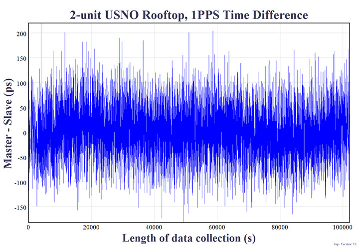
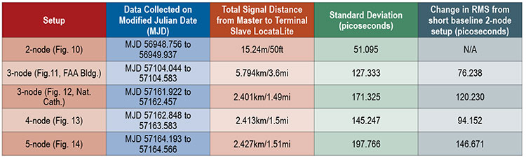
Figure 10. Two-node setup on USNO rooftop, collected for slightly more than 1 day. Distance: 15.24 m/50 ft. Synchronization Standard Deviation (SSD) = 51.095 picoseconds.Figure 11. Three-node setup at USNO and FAA Building, collected for over 12 hours: 5.794 km/3.6 mi. SSD = 127.333 picoseconds.Figure 12. Three-node setup at USNO National Cathedral, collected for over 12-hours: 2.401 km/1.49 mi. SSD = 171.325 picoseconds.Figure 13. Four-node setup at USNO with cascades at National Cathedral and USNO building 1, collected for over 17-hours: 2.413 km/1.5 mi. SSD = 145.247 picoseconds.Figure 14. Five-node setup with cascades at National Cathedral and 2 hops at USNO building 1, collected for over 8-hours: 2.427 km/1.51 mi. SSD = 197.766 picoseconds.
Results
The results in Table 1 show the 1PPS signal variability for each LocataNet under evaluation. These values represent the frequency coherence between master and terminal slave LocataLite 1PPS signals for each experiment.
Table 1. LocataNet frequency stability.
The two-node setup used two LocataLite antennas located within 15.24m of each other. The measured precision standard deviation was 51.095 picoseconds. This value is a culmination of the total Locata noise budget, which is expected to consist of TimeLoc noise, residual tropospheric error, multipath change (signal scattering/diffusion), PPS generation, and PPS measurement. This two-node result can be used as a baseline for Table 1 measurement results over longer distances. The differences are shown in the last column of Table 1. For example, cascading TimeLoc over the 5.794 km three-node setup introduced an additional deviation of 76.238 picoseconds, compared to the two-node set-up.
The three-node setup tested the effect of adding a TimeLoc cascade wherein the Locata signal from the master is routed to an intermediate LocataLite, and then to the terminal slave. When the master LocataLite signal was cascaded through the intermediate LocataLite at the FAA Building, the configuration showed a standard deviation of 127.333 ps across a total signal path length of 5.794 km. Alternatively, when the master LocataLite signal was cascaded through the intermediate LocataLite at the National Cathedral, that three-node configuration showed a standard deviation of 171.325 ps across a total signal path length of 2.401 km.
Interestingly, it appears that in the two different three-node setups, the intermediate cascade to the FAA building (2.9 km from the master and terminal slave LocataLites) delivered slightly better time transfer performance than the configuration which leveraged the closer (1.183 km) National Cathedral intermediate cascade. We believe this is attributable to the fact that the line-of-sight between USNO Building 78 (the site of the master and terminal slave) and the National Cathedral (the intermediate cascade) was completely obscured by heavy foliage seen in Figure 9, and that this particular configuration required the signal to pass through the foliage twice when being transmitted back and forth. Not only does foliage introduce multipath, but the properties of this foliage also changed regularly according to wind and moisture — two weather attributes that varied significantly over the course of the week in which those particular experiments were set up and run. This theory seems reasonable, since the four-node setup only required the signal to pass through this foliage once, and the recorded performance was better than the three-node setup — despite the fact that an additional TimeLoc cascade point was introduced.
The four-node setup included TimeLoc cascades at USNO Building 1 and the Washington National Cathedral. In this configuration, the data from Table 1 shows a standard deviation of 145.247ps across a total signal path length of 2.413 km.
The five-node setup included yet another TimeLoc cascade between the National Cathedral and Building 1 at USNO before reaching the terminal LocataLite slave. In this configuration, the data from Table 1 shows a standard deviation of 197.766ps across a total signal path length of 2.427 km.
Frequency Stability
Frequency stability is best measured over long periods. Because all of the equipment in the two-node setup was located on USNO premises, it could be run undisturbed for a longer period of time than configurations which required access to external facilities outside of the USNO’s control. Data obtained from the two-node setup were used to calculate the frequency stability between the two TimeLoc’d LocataLites. The length of this data set was 28 hours, 22 minutes, and 40 seconds. During this period, the approximate one-day frequency stability was measured as 1×10-15 (1 part per quadrillion).
To put this measurement into a more practical context: Stratum 1 is defined as a source of frequency with an accuracy of at least 1×10- 11, hence Stratum 1 performance generally originates from an atomic standard. For example, Cesium beam atomic clocks typically provide better performance than this, with one day Allen deviation stabilities in the mid- Ex10-14 (usually stable to between 3×10-14 to 6×10-14). Rubidium clocks are typically never more stable than 1×10-13 and Maser clocks are typically stable to mid-to-low Ex10-15 over one day.
Locata’s link stability — achieved without the use of atomic clocks — is clearly capable of distributing Stratum 1 frequency and precise time without substantially degrading the reference clock stability. This measured performance is significant, because a stable network is an essential prerequisite for precise time and frequency transfer. Moreover, for many traditional timing applications and developing digital and IoE applications, stability is more important than accuracy; just as for most advanced technology applications, frequency is more important than time of day.
Conclusions
The five USNO experiments suggest that the variations of the measured frequency synchronization between master and terminal slave LocataLites were not inevitably attributable to the distance between LocataLites, but rather governed by the number of nodes or cascade points in the LocataNet configuration, and LocataLite signal quality. Each signal cascade through an intermediate LocataLite introduced ~25ps of jitter into the solution.
Additionally, it was noted that transmitting TimeLoc signals across an urban environment did not always allow for unobstructed line-of-sight or completely open-sky environments. For instance, some of the LocataNet configurations required the signal to travel through dense, leafy trees which appeared to slightly affect overall frequency stability. Additionally, one FAA configuration required the signal to travel indoors through a tinted window which ultimately affected received signal strength.
These USNO tests highlighted the capability of the LocataLite as a viable option for a stable 1PPS distribution setup within an urban environment in support of applications like cell tower synchronization in “GPS-challenged” environments. All tested configurations demonstrated frequency synchronization of less than 200 picoseconds. This is significantly better than any other known wireless network synchronization methodology, including GPS. Furthermore, if clear line-of-sight is available between a master and slave LocataLite, the 2-node precision has been shown to be on the order of 50ps, and has one-day stabilities to 1×10-15.
These results, reinforced by those previously reported in University of New South Wales tests over a very large area, suggest that distance between nodes is not a significant factor, provided that sufficient signal quality is maintained. Thus, there are no theoretical or technical problems with scaling LocataNets to very large areas. In fact, this has already been demonstrated at the White Sands Missile Range where the USAF has now deployed a fully-operational Locata network that covers up to 2,500 square miles (6,500 square km), about 80 times the size of Manhattan.
The USNO trials reported here have clearly demonstrated TimeLoc’s relative picosecond-level synchronization of independent Locata networks. If this highly-stable network capability were not in place, precise time transfer would not be possible. The next step is to demonstrate how well a LocataNet can deliver absolute time transfer of the USNO’s Master Clock time to any other network node across similar areas of Washington, D.C.
Acknowledgments
The authors would like to thank James Shepherd of the National Cathedral and Paul Worcester of the FAA for use of their respective buildings. The authors would also like to thank Locata personnel for the use of their equipment and technical assistance in setting up the LocataNets under evaluation.
This article is based on a paper presented at ION GNSS+ 2015.
Disclaimer
Though particular vendor products are mentioned, neither official USNO endorsement nor recommendation of any product is herein implied.
Edward Powers is the GNSS and Network Time Transfer Operations Division Chief at USNO. He also serves as an advisor to the USAF GPS Directorate supporting space atomic clock development, modernized GPS III navigation message design, GPS accuracy improvement studies, and GPS UE development.
Arnold Colina is an electronics engineer in USNO’s GNSS and Network Time Transfer division, tasked with providing accurate UTC reference through GPS and performing calibration tests on GNSS receivers.
Timing Versus Synchronization
“They say “timing is everything” but nowadays it’s probably more correct to say “synchronization is everything”. There is a significant difference, yet many are surprised to learn they are not the same thing.
“Time dependent” applications rely on their clocks being close to the “real time”, as defined by a consensus of super-accurate atomic clocks managed by national bodies like the USNO. Once agreed upon by the labs, this “real time” can be distributed to various “time dependent” networks as a reference time to drive their operations.
“Time synchronized” applications, on the other hand, employ a methodology in which a common network time can be transferred to each network node. In other words, often the real technology enabler is that all the clocks in a defined network are synchronized to each other, even if they all run to what is any arbitrarily defined time-base. The “real time” doesn’t matter as much as how closely the node times agree with each other. As Einstein famously taught us: “Everything is relative.”
For example, accurate synchronization enables GPS positioning to work because a user’s GPS receiver relies on time-of-arrival comparisons from four or more satellites transmitting their signals at the same instant. But — even in this GPS paradigm where atomic clocks are always touted to be the most fundamental of requirements — it is important to appreciate this: A GPS user’s receiver does not care how, or to what “time,” the satellites are made synchronous. The only things the user receiver needs to know is where the satellites are, and that the satellites are synchronized when they transmit their signal.
Unfortunately sustaining high-precision, reliable time synchronization of multiple network nodes is a mammoth engineering task. Just ask the US Air Force! All clocks, no matter how accurate they are, eventually drift, so they cannot remain synchronized without comparison and adjustment.
Given the world’s exploding, insatiable demand for more data transmitted via ever-faster wireless systems, synchronization will become even more important than it is today. More wireless users and more bandwidth per user means that nanosecond — or even picosecond — network synchronization is one of the emerging engineering challenges of the 21st century. There are few resource on earth which are as scarce, or more precious today, than spectrum. So there is no question that better or cheaper ways to greatly improve network frequency and synchronization will translate directly into better use of the world’s exceptionally valuable, extremely limited spectrum resource.
BYOD Sub-Meter Positioning for Mapping and GIS Professionals
Employees bringing their own mobile phones and tablets to their jobs in the field enables them to complete more tasks using fewer devices. However, this practice introduces operational and security vulnerabilities.
By Matt van Doorn
In the mapping and GIS industries, mobile devices such as smart phones and tablets have a growing presence in the field; they enable businesses to work smarter and more efficiently. The Bring Your Own Device (BYOD) trend — essentially the use of commercial-grade devices for work purposes — will likely not slow down. BYOD is not without its pain points. Organizations face many security vulnerabilities when commercial-grade devices access critical data via corporate IT networks. Additionally, there are applications where a mobile device’s location capabilities are not accurate enough for GIS professionals to efficiently and effectively locate an asset and collect data.
Company IT departments have multiple options that control and monitor access to combat BYOD security issues; however these options do not resolve the accuracy issue. Traditional company-issued handheld integrated receivers for data collection are designed to meet accuracy demands in almost any physical environment condition. While these devices are the most appropriate technology option for some applications, they tend to be expensive for the positioning tasks where a smart phone or mobile device is “good enough.”
What to do when better accuracy on a mobile device is required, but it doesn’t make sense to invest thousands of dollars in a traditional receiver? With proper research, field professionals will find professional solutions that pair with consumer-grade smart devices to produce the requisite accuracy for a fraction of the cost of a traditional receiver.
Requirements and Accuracy
At a minimum, handheld receivers destined to work in conjunction with mobile devices must meet the following requirements:
The device must have moisture ingress protection to function properly in snow, ice, rain or dust environments.
The device must survive falls in hard terrain. It should have shock, drop and vibration protection.
The device must last the full workday for the professional to complete all workflows on a single battery charge.
Legacy company-owned receivers typically meet the requirements above and have had a long-term reputation for accurately providing positioning data. These devices are still the appropriate solution for environments where it does not make sense to take a smart device, such as a remote location in rough terrain where the smart device may not perform.
However, a smart device can in many cases enable the employee to be more efficient. Thanks to the accessory market, many of the above-listed requirements can be easily addressed. For example, smart-phone juice packs can fix the battery longevity issue; cases can protect against weather, shock or dropping; and screen covers can address the sunlight screen visibility issue. With a smart device in hand, GIS and mapping professionals not only have access to GPS data, but they are able to access and complete other work-related tasks from the same device such as email, internet access and voicemail. Plus, a smart phone is only a fraction of the cost of traditional receivers.
The most critical component that smart devices still cannot address is sub-meter accuracy, which many mapping and GIS professionals require to successfully do their job.
Accuracy Drives Cost. Mapping and GIS businesses are acutely aware of the efficiencies created by greater accuracy. With poor information, errors become increasingly costly. When robust, accurate data is collected, there is a direct correlation to improved workflows and operations. This allows professionals to be more strategic in ensuring that applications are effective and efficient across operations.
Aerial and satellite imagery made initial steps toward generating more accurate data collection, bringing mapping and GIS professionals to within a 50-centimeter range of the assets. Subsequently, high-speed lidar collection tools, designed to capture large areas at 5–10 cm accuracy, came to the market. While these tools significantly improved data collection, precise measurement typically requires more time, more expense and highly specific instruments in order to generate more data.
Today, handheld receivers can achieve high accuracy without using survey-grade tools, in applications that include:
Mapping: Any application, including locations, quantities, densities, specific areas and map change.
Aquatic monitoring
Buried utility infrastructure/cable location
Water/wastewater disposal
Location and elevation measurements: for example, elevation data on manholes or trunk lines.
Requirements vary across applications and industries. The mapping/GIS professional must determine the level of accuracy their workflow requires.
Accuracy Evaluation
A typical smart device, properly assisted, can achieve an accuracy range of up to 5–6 meters when used to locate an asset. In many cases this is good enough. To obtain positioning data, iOS devices use the application “Location Services,” which is available on multiple mobile platforms. Location Services enables location-based apps and other applications to use information from GPS and cellular and Wi-Fi networks to determine location information. The location provided by a hybrid system with cellular-assisted GPS (A-GPS) allows the device to identify location within a 5–6 meter range of an asset. Wi-Fi positioning alone can determine a location with an accuracy of about 74 meters, and cellular positioning alone offers about a 600-meter range for location, according to industry sources (www.windowscentral.com/gps-vs-agps-quick-tutorial).
However, cellular positioning can be limited when there is no network available. In remote or industrial settings, this could create difficulties in asset location. In water/wastewater, for example, when a GIS professional is in a ditch looking for a valve or a meter and there isn’t a network connection, the accuracy level provided without GPS may not be sufficient for that application. When A-GPS is not available due to a lack of cellular network, GIS professionals also have to deal with convergence time.
Another example involves searching for a manhole cover when the ground is covered by a couple feet of snow. In this case, the 5-6 meter range is quite large and could lead to a lot of time spent digging until the manhole is uncovered. This wastes time and energy, and leads to higher costs. Some receivers have the sub-meter capability and can provide the location data directly to the professional’s consumer-grade smart device through Bluetooth. By simply pairing the receiver with a cellphone, the GIS professional can quickly locate the asset, collect data and move on to the next task.
Accuracy Solutions
Location shortcomings in consumer-grade devices generally boil down to antenna performance. Consumer-grade smart devices are designed for exactly that: consumers. With antennas for Wi-Fi, Bluetooth and GPS built into the small device, there will be compromises in location accuracy. When location must be pinpointed, an integrated handheld receiver can enhance accuracy. Receivers are readily available with 12 channels parallel tracking. Some receivers can also support multiple satellite constellations, including GPS, GLONASS, Galileo, Beidou, and QZSS with up to 44 channels of parallel tracking. The accuracy of these devices is further supported by augmentation: WAAS, EGNOS, MSAS and GAGAN. These receivers can provide sub-meter accuracy, with asset location with as close as 60 centimeters. Some devices also support Virtual Reference Stations (VRS) and Trimble’s Real Time eXtended (RTX) correction service for sub-meter accuracy. Some RTX services achieve real-time sub-meter accuracy with IP and cellular connectivity, or over satellite L-band.
A receiver that integrates with the workflows of various mapping and GIS softwares as well as third-party applications will pair up nicely with a mobile device. The computations are all done for the professional, and will transmit signals via Bluetooth into the host devices using NMEA protocol. On iOS and Android devices, the location is available through the Location Services API. Third-party applications are also able to work with the receiver through consumer-grade devices that utilize the location services API. Some receivers are available across operating systems including iOS, Android and Windows, and are available to upgrade to the latest smart device whenever needed.
Important Device Attributes
Receivers designed to be compatible with a variety of smart devices can be shared among multiple devices. When it is time for a smart device upgrade, the new device can easily integrate with the receiver. Additional features that make these receivers especially convenient to use in the field include:
Small size: Mapping and GIS professionals don’t always have an extra hand available to carry an extra device. If it can fit in a vest, jacket pocket, pouch, clipped onto a belt, or pole mounted it will function in many scenarios.
Lightweight.
Rugged: Some receivers comply with MIL-STD-810 ruggedness with IP65 rating for shock, drop and vibration.
Battery life: for field performance for a full work day.
External antenna port: An accessory port for external data if the collecor needs to be mounted on top of a vehicle, or in a hard hat situation; a bonus feature worth consideration.
BYOD Trend and Limitations
The smart-device market will not cool down anytime soon. Gartner Research predicts that in 2015, almost 2.3 billion devices will be shipped worldwide. Whether these smart devices are provided by the company or truly BYOD, they will need to be augmented to effectively serve the applications they are intended to support. Solving the security issue can have a bearing on whether a company chooses to let employees use their own device or provide one; either way, enhancing the location capabilities of the device can be easily achieved with accurate receivers.
Matt van Doorn is a product management, product marketing, market management and business development professional at Trimble Navigation. He has years of experience in the data communication and telecommunication industry with deep knowledge of international markets.
GPS landforming is the reshaping of a fields topography to predesigned 3D surfaces using high-accuracy GPS to control the blade height of the earth-moving machine. It is typically done to improve surface drainage and water infiltration uniformity.
Davco Optisurface, the company that developed the 3D landform design software OptiSurface Designer, has seen strong adoption as the concept catches on. The software has been used to design more than 400,000 acres, according to Arkansas-based global sales manager Preston Marthey.
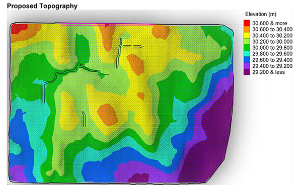
WM-Form. Trimble launched a GPS landforming software program in February. WM-Form enables growers and contractors to turn their fields into optimal surfaces, even in areas that could not be leveled before, Trimble said.
“With more farmable land that is optimized for water management and more uniform production, growers can experience increased yield,” said David Fitzpatrick, Water Solutions business area director for Trimble’s Agriculture Division.
Trimble’s product is designed to work with its WM-Topo survey system and Trimble FieldLevel II system. WM-Form has surface design tools and flexible parameters so growers and earthworks contractors can use it to repair underperforming areas and extend the amount of productive farmable land. It can reduce the volume and cost of earthworks and minimize disturbance to valuable topsoil. Growers can optimize water distribution and drainage, reduce erosion and flooding by effectively directing waterflow, and create more uniform crop production that can lead to increased yield.
Growers can analyze topographic data in WM-Form to identify surface problems limiting yield potential and create a design that optimizes their field’s surface. The software also provides reports for volume, area and constraints, providing an accurate quote on the total cost of the project.
Horizon. Topcon’s Horizon software is an icon-based, user-definable system that presents a choice of views for each function you perform. It runs on all three of Topcon’s X family of precision agriculture consoles. With Horizon, growers can set autosteering patterns, control application rates, monitor operations, and map every pass — and a new feature allows for water management.
“Water conservation…is designed to provide the ability to perform land forming while also offering GNSS auto steering of the tractor,” said Neal Toso of Topcon Positioning. Using the Topcon X30 and AGI-4, water conservation and land forming users can level fields while auto-steering to maximize efficiency and reduce the amount of material moved, he said.
“With the X30 console, using Horizon software, connected to Topcon MC-R3 blade control, it is easy to take the output from Topcon AGForm 3D design software to produce accurate modeling and land forming. This allows proper drainage to occur, resulting in a healthy, productive crop,” said Toso. “Together, these Topcon products are designed to provide a turnkey approach to superior landforming operations.”
In Costa Rica, Jose Maria Aguero, CEO-director general of Agricultura Cientifica S.A., now uses Horizon. Aguero first employed laser leveling in the late 1970s. “We started noticing that rice and other crops produced less in areas with deep cuts from laser leveling because we had cut the more fertile topsoil off,” Aguero said. “But it was the only tool we had, so we kept doing it.”
Then Aguero discovered Topcon’s GPS land forming products. “Sugar cane crops are expanding dramatically in our area, and the operators don’t use irrigation. Water management is needed to improve drainage because in the rainy season it is too wet, which affects crop development. The only way the cane companies can get sugar cane into a new growing area is with GPS and 3D landforming,” he said.
“GPS with 3D landforming only moves 250 to 300 cubic meters per hectare,” Aguero said. Compared to laser leveling, “That is more than a 90 percent reduction in cost. And, moving less soil keeps more of the fertile top layer in place to promote fertility.”
Landforming Lessons
Surface drainage and irrigation problems can be solved with GPS landforming at low cost, agricultural engineer Graeme Cox says. This is proven with many crops and farming styles, irrigated and non-irrigated.
Cox has learned the following about GPS landforming, based on his experience around the world.
Water is king. Eighty percent of yield variability and profit loss is due to too much, or too little, water. Yield maps show this. “Focus on optimizing water management first,” Cox said.
Ponding kills profits. If water is standing in fields 24 hours after rainfall or irrigation, it is killing profits. “Expect eight percent per day yield loss plus nitrogen loss, increasing pest and disease, delaying planting, spraying and harvesting.”
Subsurface tile drainage is good, but expensive. “Tiling typically has a lower return on investment than GPS landforming and does not work well on heavy soils or those with limited elevation relief,” Cox said.
Ditching is good. “But,” he adds, “it can be a pain if ditches take out valuable crop area or restrict machinery access.”
Lasers are dead. Lasers only work in a straight plane. GPS allows farmers to follow curved topography with curved design surfaces.
Earthworks and topsoil movement can be reduced up to 80 percent with landforming designs and GPS machine control compared to other methods, Cox claims.
Two new products from GPSTrackIt.com offer users of their Fleet Manager vehicle tracking, fleet and workforce management system new tools for navigating, routing and communication.
Field Service Manager provides access to Fleet Manager’s route planning and navigation system. New stops can be pushed out to the tablets from dispatch. It enables drivers to add stops to their route on the fly. Push notifications also alert the driver to incoming messages, regardless of which page in the app they are currently viewing.
GPSTrackIt Forms takes the communications component of the FSM to a new level. This tool provides the ability to quickly create forms to capture everything from text to photographs to signatures.
“The new forms tool is really powerful,” said Eddie Bermudez, GPSTrackIt.com’s product development manager. “Part of it’s power is the ease of use. The different field types are created by clicking a button and adding a field label. It’s that easy.”
GPSTrackIt Forms provides unlimited forms. Form data can be captured offline and updated later. The tool provides 24 preset field types, including text, video and a document viewer.
“The forms aren’t just dumb collectors, either,” added Bermudez. “There’s a rules engine that facilitates skip logic and branching. And the forms can have embedded formulas and perform advanced calculations, including formula-based form scoring.”
The form tool can also export data to Excel, PDF, CSV, and JSON formats. “These two tools combined provide drivers and the back office with an amazing array of opportunities to collect data about their customers, as well as their own customer service,” Bermudez said.
The Averna RP-6100 Multi-Channel RF Record & Playback for RF application testing allows users to tecord real-world signals such as GNSS, HD Radio, LTE and Wi-Fi — plus impairments — to significantly advance projects and harden product designs. Skydel Solutions’ GNSS simulator is an entirely software driven innovative and cost-effective simulator that works with the RP-6100, enabling users to test corner cases and future events with a real-time GNSS solution.
PCTEL’s GPS/GLONASS high-performance asset tracking and synchronization helix antennas are now available commercially. The antennas capture the frequencies needed for GPS, Galileo and GLONASS satellite reception. This cross-compatibility allows global OEMs to use one standard platform to serve both European and U.S. markets.
PCTEL uses its proprietary filtering design to allow wideband coverage while achieving superior out-of-band rejection. With an IP67 rating, the small form-factor helix antennas will withstand harsh environments.
AsteRx-U and AsteRx-U Marine multi-constellation dual-antenna receivers incorporate the latest GNSS tracking and positioning algorithms and interference mitigation. Machine-control users in the agricultural, construction, marine and mining industries benefit from a complete system with integrated UHF radio, Wi-Fi, USB, Bluetooth and cellular connectivity and a spectrum analyzer. All configurations can be done via the on-board web interface.
The AsteRx-U has decimeter- and centimeter-level RTK positioning including TerraStar. The AsteRx-U Marine also supports Veripos PPP augmentation services.
The RTG2 is a GNSS constellation simulator that generates realistic GNSS RF signals, taking into account current and future GNSS constellations. RTG2 is able to entirely simulate one or many constellations (GPS, Galileo, etc.) including satellite-based augmentation systems such as WAAS and EGNOS.
The generator is entirely configurable (troposphere and ionosphere effects, simulated receiver trajectory, etc.) through a user-friendly interface accessible on a separate PC through Ethernet. RTG2 is highly flexible and scalable, offering hardware and software upgrades for capability extensions.
Telit’s Jupiter SE873 GNSS receiver with flash memory.
GNSS Receiver with Flash Memory
The Jupiter SE873 GNSS receiver is a complete multi-constellation position, velocity and time engine that delivers versatile performance in harsh environments. The 7 x 7 x 1.85 mm module has serial quad I/O flash memory, an integrated low noise amplifier, SAW filter, TXCO and real-time clock. The Jupiter SE873 supports Assisted GPS (both autonomous and server-based) plus SBAS, which improve time-to-first-fix and position accuracy. AGPS data is stored in flash memory and is available even after all power has been removed and then restored. This is especially important for battery-operated equipment.
The SE873 supports the entire GNSS spectrum: GPS, GLONASS and BeiDou, and it is Galileo ready. It delivers simultaneous low-power tracking of GPS and GLONASS or GPS and BeiDou.