Sensor Modeling and Sensitivity Analysis for a Next-Generation Time-Space Position Information System
By Mark Smearcheck and Michael Veth, Air Force Institute of Technology
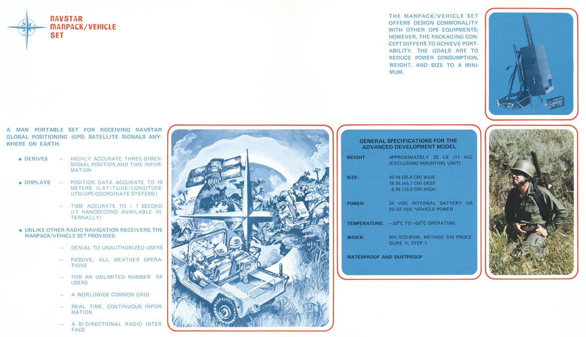
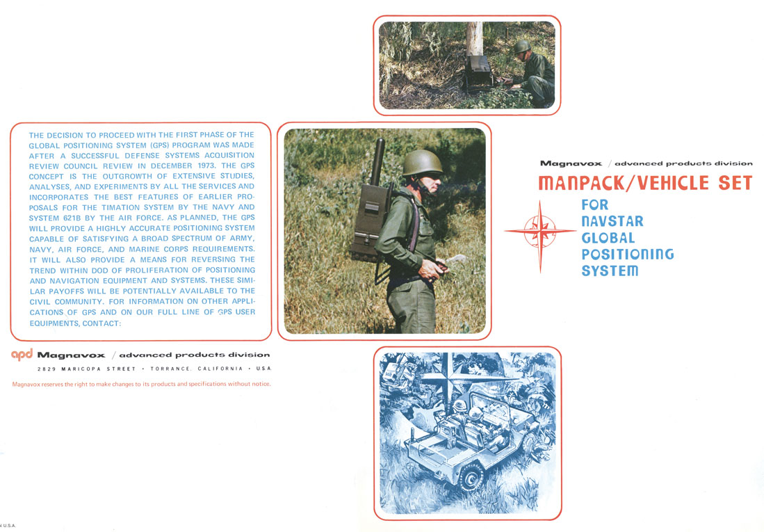
Increasing availability and performance of state-of-the-art navigation sensors motivates the need for a highly accurate reference system commonly referred to as a time-space position information (TSPI) device. The Advanced Navigation Center at the Air Force Institute of Technology is working with the Air Force Flight Test Center to develop a next generation time-space position information (TSPI) system to be used for test and evaluation of modern navigation devices.
TSPI systems such as the GPS Aided Inertial Navigation Reference (GAINR) or Advanced Range Data System (ARDS) accompany navigation sensors during flight testing to collect the precise position, velocity, and attitude. Current GAINR TSPI performance levels include 1.0 m of position uncertainty, 0.1 m/s of velocity uncertainty, and 1.75 mrad of attitude uncertainty. Goal performance levels for next-generation TSPI call for an order of magnitude improvement over current systems.
A more accurate test and evaluation device will likely require fusion of multiple sensors of varying modalities such as GPS, inertial, electro-optical and infrared cameras, laser range sensors, barometric altimeters, ground-based theodolites, and ground-based tracking radar. This research aims to identify an integrated sensing package and the sensing techniques required to achieve the next generation TSPI accuracy.
In order to accomplish this task, a sensitivity analysis is performed that predicts the quality of the navigation solution attainable using various external sensor combinations. The sensitivity analysis requires sensor characterization and modeling in addition to development of a software simulated world (the flight test range) that the sensors are able to observe. Issues also investigated in this research include vision-aiding techniques, optical feature deployment, and testing in GPS-denied scenarios.
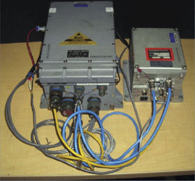
The GPS Aided Inertial Navigation Reference (GAINR) system consists of a Honeywell 764-G embedded GPS/INS with a custom control and recording unit. The data are post-processed using an optimal smoother and differential GPS measurements.
Sensors and Simulated World
The Air Force Flight Test Center currently obtains TSPI using the GAINR, which includes a navigation grade inertial measurement unit (IMU) and dual-frequency code-based differential GPS (DGPS). Carrier-phase GPS, if available, could be implemented to increase position accuracy.
When integrated into a highly dynamic platform, such as tactical fighter, a kinematic solution may not always be obtainable due to difficulty resolving integer ambiguities and cycle slips experienced in the receiver’s tracking loops. The sensitivity of both code and carrier-phase differential GPS is included in this research due to the uncertain availability of a kinematic solution.
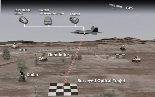
Scenarios of GPS denial are always an area of concern for the warfighter, and thus GPS-independent test-platforms must be examined. Other positioning sensors, useful in GPS-denied testing, include ground-based theodolites and radars. These devices are installed at surveyed locations on the test range and are used to track the test aircraft. Theodolites are pivoting platforms that may contain various sensors and provide range, azimuth angle, and elevation angle measurements. Radars are also used to provide the same type of measurements, along with an additional velocity measurement (Figure 1).
Figure 1. Overview of possible TSPI sensors. The sensors consist of both aircraft-based and ground-based devices.
Onboard optical sensors including high-resolution digital cameras and laser range finders have also been investigated for TSPI use. This research proposes to install surveyed targets on the test range that are easily identifiable through feature extraction and tracking methods such as the scale-invariant feature transform (SIFT).
Cameras are able to observe position and attitude through homogenous pixel location measurements of image features (FIGURE 2).
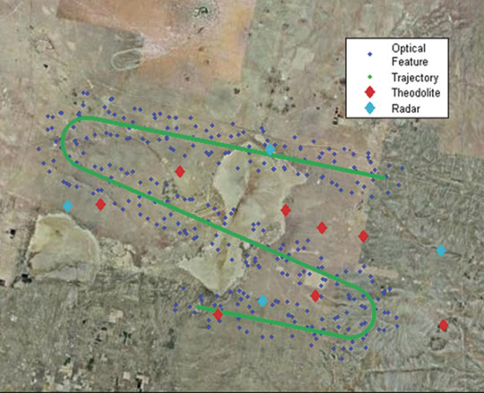
Figure 2. Simulated test range at Edwards AFB that includes optical targets, ground sensors, and a flight test profile. Optical landmarks are randomly spread within the field of view of the optical sensor over the trajectory.
An objective of this sensitivity analysis is to show the attitude performance achievable through feature tracking of surveyed targets. When image-aiding of an IMU is implemented in a navigation filter, such as the extended Kalman filter (EKF), next generation TSPI level attitude accuracy should be reached.
The other optical sensor investigated, the laser range finder, is used to augment the navigation solution by measuring distance to the surveyed targets detected by the camera.
For the sensitivity analysis a simulated world is generated for the sensors to make observations. The world simulation includes GPS ephemeris, a digital terrain elevation database (DTED), gravity models, natural terrain landmarks/targets, manmade targets, a ground sensor deployment map, simulated flight test profile, and vehicle sensor installation lever-arms.
Sensitivity Analysis
The goal of the sensitivity analysis is to determine the minimal set of sensors that will meet next generation TSPI performance requirements. Sensor models and world characteristics are used to calculate expected position, velocity, and attitude uncertainty given a particular trajectory, sensor package, and feature set. The aircraft’s state vector, , as a function of the measurement, z, and uncertainty matrix, R, is represented as
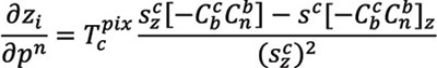
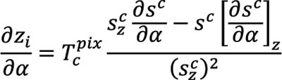
where H is the observation matrix. The observation matrix is a Jacobian made up of partial derivates of each sensor’s measurements with respect to position, velocity, and attitude. Example H matrix elements include the partial derivates describing the camera measurements with respect to position and attitude. The partial deviate of the pixel coordinate, zi, of an image feature with respect to position, pn, is
where Tcpix is the camera frame to pixel frame transformation matrix made up of calibration parameters, sc is the line of sight vector from the camera to the target expressed in the camera frame, Cnb and Cbc are direction cosine matrices, and the subscript z denotes the z dimension of the indicated navigation frame. The partial derivative of the pixel coordinate of an image feature with respect to attitude, α, is calculated as
The H matrix’s partial derivatives describing observations from other navigation sensors are derived in our previous
work, “Sensor Modeling and Sensitivity Analysis for a Next Generation Time-Space Position Information (TSPI) System,” Proceedings of the ION International Technical Meeting, 2010. The a posteriori uncertainty of the state or sensitivity, P, at time k is calculated as
where P0 is the initial uncertainty.
Results
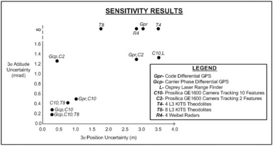
Results show the three sigma median uncertainty of position and attitude for various sensor combinations over a common flight profile through the test range (Figure 3).
Figure 3. Sensitivity analysis results of position and attitude with various sensor combinations. Scenarios of unobservable attitude are designed by the infinity symbol.
Conclusions
The sensitivity analysis indicates that the most practical sensor package that meets next-generation TSPI performance is the combination of carrier-phase GPS and a high-resolution camera tracking ten SIFT features per image.
In this example, tracking only two SIFT features per image does not provide the necessary level attitude accuracy, although incorporating inertial measurements is expected to reduce the overall number of features required per image.
In the absence of GPS, theodolites when coupled with a camera can function as a reasonable alternative. It should be noted that since the sensitivity analysis relies on a simulated world the feature tracking performance and target surveying accuracy may change during operational testing.
The next phase of this research is to integrate the sensors with an IMU using an extended Kalman filter. Fusion with a navigation-grade INS is expected to improve position, velocity, and attitude accuracy.
If simulated results are promising, the next phase of the effort will focus on collecting flight test data to validate the simulation and further increase the fidelity of the simulation.
Acknowledgment
The authors would like to thank the Air Force Flight Test Center for supporting this research.
MARK SMEARCHECK is a research engineer with the Advanced Navigation Technology Center at the Air Force Institute of Technology (AFIT) at Wright Patterson Air Force Base in Dayton, Ohio. He received his B.S. in electrical engineering in 2006 and his M.S. in electrical engineering in 2008, both from Ohio University. His research topics include micro-air vehicles, indoor navigation, image-aided navigation, pseudolites, and test range instrumentation.
LT. COl. MICHAEL VETH is an assistant professor of electrical engineering at AFIT and deputy director of the Advanced Navigation Technology Center. He received his Ph.D. and M.S. in electrical engineering from AFIT and his B.S. in electrical engineering from Purdue University. He is a graduate of Air Force Test Pilot School.
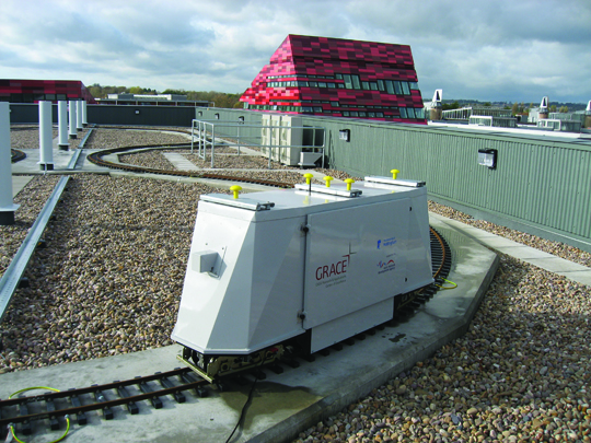
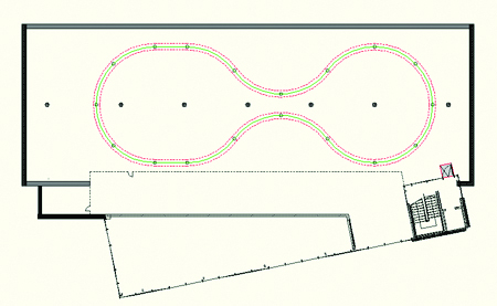
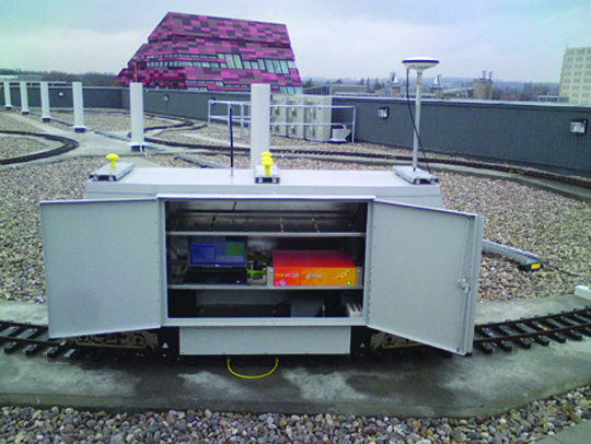
One-hundred-twenty meters of test track, designed for repeatable dynamic position testing, run along the roof of the new Nottingham Geospatial Building at the University of Nottingham, UK. The figure-eight track provides an optimal controlled environment with test equipment aboard a remote-controlled, multi-sensor 7¼-inch gauge locomotive platform with a top speed of 7 kilometers per hour, a dedicated power supply, and five antenna mounts. Simulation of the track using Spirent GSS8000 hardware (GPS and Galileo) provides additional planning and testing capacity.
The combination of these tools creates the ideal environment for our new project: augmentation of GNSS systems with ground-based Locata positioning technology. This pseudolite-like system, described in the March issue of GPS World, works in a GNSS-like fashion, using code and carrier phase. The major advantage, apart from utilization of the licensee-free 2.4 GHz frequency band, is the precise time synchronization of the network to the nanosecond level.
The proposed integration addresses Locata’s weak vertical coordinates (due to relative coplanarity of transceivers) and GNSS’s requirement for a clear view of the sky and location-specific weak geometric distribution of the satellites. Prior research and analysis suggests considerable improvement in 3D positioning accuracy when combining ground-based positioning devices (pseudolites) with GNSS, but the current project pushes the research forward by attempting to create on-the-fly ambiguity resolution.
Combination of hardware and software simulation has provided an initial assessment of the proposed integration, optimization of equipment location, and test of the mathematical model to be used. Practical tests, using the roof lab on top of the NGB, will further verify the method and allow comparisons between the predicted and real-life results. This will aid the assessment of noise, multipath, and in-bound interference. The test design minimizes the tropospheric effect, while track flexibility and repeatability offer the possibility of implementing and simulating obstructions and areas of GNSS outage. This will provide a full assessment of the mathematical model and the integrated system’s capacity.
This project offers new opportunities in civil engineering, specifically monitoring and machine control. GPS is currently widely used for those applications, with Locata also proven successful. The integrated solution can provide not only enhanced positioning capacity but lower the required number of visible GNSS satellites, and offer improved integrity and quality control, ultimately increasing the safety of life.
The intended utilization is for positioning in dense urban areas and essential structures (airports, seaports, factory sites, bridges) where sky visibility or correct satellite distribution cannot be guaranteed.
The track is available for other projects. Funded by East Midlands Development Agency, hosted by the Institute of Engineering Surveying and Space Geodesy, the Centre for Geospatial Science, and the GNSS Research and Applications Centre of Excellence (GRACE).
There’s something I’ve been wanting to write about since the ION-GNSS conference a few weeks ago. However, a nasty cold, a 10-day trip to Europe (INTERGEO conference), and some jet lag have kept me from it until now.
Here goes.
First of all, most of the presentations from the CGSIC meeting are available on the USCG Navigation Center website. You can view them by clicking here. There’s some very good reading and most of it is pretty light-weight and in PDF format.
One of the presentations at the CGSIC (Civil GPS Service Interface Committee) meeting during the ION-GNSS conference was “Integrating NDGPS and SBAS —
An Optimal Real-time GPS Mapping Solution,” presented by Jean-Yves Lauture of Geneq, Inc.
I’m publishing two of the slides from his presentation in order to:
Show the accuracy potential of WAAS and NDGPS given a high performance L1 receiver.
Discuss the statistical names/values used to express GPS accuracy.
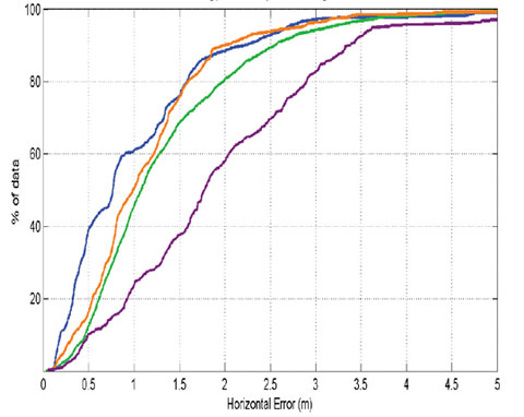
First of all, each of the slides below are at the same scale. Each ellipse is 20 cm with the outside limit (radius) being one meter.
I’ve known for quite sometime that SBAS (WAAS in this case) is capable of sub-meter precision with a single-frequency GPS receiver. These results are a bit better than what I’ve seen personally, and keep in mind it’s a limited data set of 1,800 continuous epochs, but impressive none the less. Also, keep in mind that the WAAS Performance Analysis Report published quarterly by the FAA’s National Satellite Test Bed shows the 95% horizontal accuracy value for Denver, Colorado, (near where this data was collected) being .547 meters for the quarter ending June 30, 2010 (7,856,354 samples collected over three months).
30 minutes of WAAS-corrected data (each ellipse represents 20cm)
The results I didn’t expect were the slide below, which shows NDGPS-corrected results using the same receiver/antenna. Keep in mind this is a GPS L1 receiver using phase-smoothed pseudorange measurements, not a GPS L1/L2 receiver using a carrier-phase float solution. If you look closely, you’ll see it states the baseline distance is 200 km. Granted, this is a limited data set, and I’ll be interested in seeing further results. If this was a dataset presented by a manufacturer or other party with some sort of interest, I wouldn’t publish it, but this is data collected by an objective entity (a credible U.S. government agency) so that earns, in my mind, a level of credibility.
The results are pretty impressive. All data points fall within ~20 cm.
30 minutes of NDGPS-corrected data (each ellipse represents 20cm)
Keep in mind that this data was collected recently, and we are currently in a period of low ionospheric activity. In other words, data was collected under near-ideal conditions. At the end of the day, my point is that GPS L1 accuracy using SBAS and NDGPS has gotten pretty darned good.
Accuracy Statistics
The second reason I’m publishing the slides is to discuss accuracy statistics.
Look at the small box inside each slide showing 99%, 95%, 68%, and 50% accuracies.
If you look at the data points, it might not be immediately apparent how those values were arrived at. For example, how could a group of data points all within ~20 cm have a 95% confidence of 37 cm?
To explain this, there was a good article published in GPS World in 2007 titled “GNSS Accuracy: Lies, Damn Lies, and Statistics” by Frank van Diggelen. It does a good job explaining statistical expressions (RMS, 2DRMS, etc.).
Keep in mind that most manufacturers express horizontal GPS accuracy specifications based on 68% confidence. When the specification sheet states “sub-meter” HRMS (horizontal RMS) precision, that means 68% of the time; the horizontal accuracy will be less than a meter. In reality, that “sub-meter” receiver won’t consistently deliver sub-meter precision. If you convert the 68% HRMS value and express it with 95% confidence (2D HRMS), the actual horizontal precision for that same receiver will be well over one meter. That’s the precision you can expect from the receiver, not the 68% confidence value.
This week, I’ve been attending the INTERGEO 2010 conference in Cologne, Germany. It’s a gathering of ~16,500 people interested in geodesy, geoinformation, and land management. It’s the largest event of its kind in the world.
Although there’s a lot of GIS activity, it’s just as much a surveying/geodesy trade show. I borrowed a little of the following from my Geospatial Weekly newsletter because I think it’s relevant in this newsletter, too. Let me just say that if you’re a land surveyor/engineer/construction contractor/GIS’r, you won’t find a trade show anywhere in the world like this one. To me, two things differentiate it from all other conferences I’ve attended that are related to surveying, engineering, construction, or GIS.
The sheer size. 16,500 people buzzing around attracting 504 exhibitors. You can find a solution to any sort of challenge you have regarding surveying, geodesy, construction or GIS. The major GNSS manufacturers (such as Trimble/Spectra, Topcon/Sokkia, Leica, Javad) have enormous exhibit booths that rival the Consumer Electronics Show (CES) held every year in Las Vegas. You don’t see these companies spending this much money to exhibit at conferences in North America.
Unlike many of the conferences I attend, the focus at INTERGEO is on the trade show exhibit area. The technical sessions are few and most are in German, so that leaves the vast majority of the attendees to flock to the exhibit area. We’re currently in Day Two of the three-day conference, and the exhibit area attendance seems just as strong as the first day, which is not typical. On top of focusing on the trade show area, INTERGEO makes it inexpensive to attend. A one-day pass to the exhibit area is only EUR 20 (~US$26) and a three-day pass to the same is EUR 48.50 (~US$63). It’s even cheaper if you buy it online in advance.
The few technical sessions held were presented by University Professors and various Ph.D.s, so although I submitted an abstract to present a paper, I knew there was no chance I’d be presenting in the formal technical sessions. The closest I am to a Ph.D. is my father’s, which he earned 40+ years ago. Anyway, INTERGEO has a stage in the exhibit area called the Trend and Media Forum. It’s sort of an infomercial stage for companies to show their products and services. They scheduled me to present on that stage, which I did earlier today (Wednesday). The title of my presentation was “GNSS is Changing a Lot — the Future of GNSS Mapping and Surveying.” The audience was sparse, but the good thing is that INTERGEO records the presentations and later posts them on their www.intergeo-tv.de site. My presentation is not on the TV site yet, but should be by Thursday. Please don’t laugh when I nearly fall down after stepping off the stage while I’m talking :-). Click on the following image to view my presentation.
Following are some pictures I took of the conference exhibit area, with captions:
There were many new product announcements in the past day. I saw one that caught my particular interest. I’ve written before that for years I relied on stand-alone satellite mission planning software. The problem that most folks have is maintaining the software as they change computers or update operating systems. There’s also the pain of having to update the almanac every month or so.
I’ve become a fan of online satellite mission planning. I’ve mentioned the NavCom Technology website a few times in this column. However, it has a few shortfalls, namely no control over the elevation mask used and no support for GLONASS or SBAS.
I’m happy to report that today at INTERGEO, Ashtech released an online satellite mission planning tool, and it seems to fit the bill. Among other things, it allows you to adjust the elevation mask, and choose to include GLONASS and SBAS satellites. Of course, since it’s an online tool, you don’t have to worry ab
out updating the almanac.
Following are a couple of screenshots from the program.
Select GPS and/or GLONASS and/or SBAS satellite
Give it a try for yourself by clicking here. There’s a really cool plot that’s generated as a 3D visualization in Google Earth, showing each satellite (green = GPS, red= GLONASS and blue = SBAS).
The use of a precise wide-area positioning technique for airborne trajectory solutions for LiDAR surveys provides both relative and absolute accuracies similar to those derived from using a local GNSS reference station.
Airborne light detection and ranging (LiDAR) surveys are among the most advanced means of producing high-resolution, accurate surface elevation models used for many applications in surveying and civil engineering. Precise geolocation and orientation (or georeferencing) of the LiDAR instrument with a combination of on-board GNSS and inertial sensors at the times when the measurements are made provides the key to high-quality elevation products.
The usual practice deploys reference GPS/GNSS land receivers in the area where the aircraft will be flying, to obtain a precise trajectory by short-baseline differential GNSS techniques. This could mean installing and operating receivers at many sites during a flight mission if the area surveyed is a large one.
We have tried a different approach: using as reference receivers those of a sparse network of Continuously Operating Reference Stations (CORS) in New South Wales known as CORSnet-NSW, and a wide-area differential GPS technique for obtaining the aircraft trajectory with sub-decimeter accuracy even with baseline lengths of several hundred kilometers. This may be comparable in precision and accuracy to the short-baseline method, but without the cost and logistical complications. This opens up a new level of operational capability, allowing flexibility for weather conditions and priority response applications.
The tests described here were organized and conducted by the NSW government’s Land and Property Management Authority, in collaboration with the University of New South Wales, in June 2009. CORSnet-NSW consists, at this writing, of 46 stations and by 2012 will provide statewide GNSS positioning infrastructure across NSW with a planned 70 stations in operation.
Precise Wide-Area Positioning
We used a technique for long-baseline differential, off-line positioning, able to deliver centimeter precision for fixed receivers and sub-decimeter precision for moving receivers. This choice was dictated by three considerations:
The intended application was the geolocation of the data of an airborne scanning LiDAR sensor to be used in the generation of high-accuracy digital elevation models (DEM).
Off-line processing, where all the GNSS data collected during the flight are available for processing and (as in this case) there is no need for immediate results, is intrinsically more reliable than real-time processing, where the data are available only up to the present epoch, and accurate results must be obtained right away, with no chance for a second try.
Differential processing makes it possible to resolve the carrier-phase ambiguities using well-understood methods.
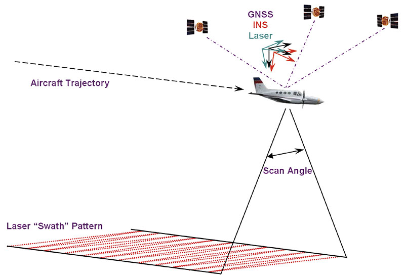
Technique. It is common practice in airborne LiDAR surveys to use GNSS both to position the instrument precisely, and to assist an inertial navigation system (INS) to obtain the orientation of the aircraft in space, as both position and orientation are needed to interpret the data properly. FIGURE 1 illustrates the relationship between the sensors used for airborne LiDAR surveys. The aircraft uses a GNSS antenna combined with an INS to georeference its trajectory. The bore-sight calibration process aligns the individual sensor orientations and standardizes the range measurements. However, if the survey is to achieve the now-expected high level of vertical accuracy (615 centimeters, 1 sigma), then the position of the GNSS/INS-derived aircraft trajectory for each laser swath must be determined with a relative precision in the order of just a few centimeters. This is achieved via differential GNSS post-processing of the kinematic airborne data together with static observations collected on precisely surveyed ground reference stations. The GNSS positions are then blended with high-frequency measurements taken by the onboard INS to produce the final trajectory and reference orientations.
Figure 1. Airborne LiDAR reference frame.
To such ends, the aircraft trajectory is usually determined by short-baseline differential GNSS, with ground receivers deployed near the intended flight path of the aircraft. In this way it is possible to use GNSS data analysis techniques that are both precise and quite straightforward to implement in software. The simplicity of these techniques is possible because, in short-baseline differential solutions, the data of the aircraft receiver and any nearby network receivers have much the same systematic errors (due to such things as satellite ephemerides errors, transmission delays, and so on) that cancel out — or nearly so — when their observations are differenced between them. This also makes it possible to resolve quickly and reliably the cycle ambiguities in the observed carrier phase, the most precise type of GNSS data, overcoming one of the main obstacles to obtaining good results. Furthermore, it is possible to get such results with single-frequency receivers, as ionospheric delay is one of the systematic effects that can be largely canceled out.
In wide-area solutions, those cancellations are not complete enough to ignore the systematic data errors, and they have to be included in the form of additional unknown parameters in the observation equations. Also, it is necessary to account for the ionospheric delays using dual-frequency data, which means using more expensive GNSS receivers and antennas.
Resolving the carrier-phase ambiguities is no longer straightforward or assured. The standard way of dealing with the ambiguities is to include them as unknowns in the observation equations and adjust them along with the other unknowns: this is often referred to as “floating the ambiguities.” Fixing (or resolving) those ambiguities to their most likely integer values in a matter of seconds to a minute is possible on occasion, when the aircraft is within less than 20 kilometers from a ground receiver, or very precise corrections for the ionospheric delay are available; otherwise slower techniques, that require tens of minutes, may be used. It is also necessary to correct as well as possible such things as the neutral atmospheric delay of the GNSS radio signals, the movement of the “fixed” stations due to plate tectonics, the solid earth tide using mathematical models, and, in the case of the tropospheric delay, estimating the error in the corrections made using a standard formula as an additional unknown per receiver.
Over the years all these difficulties have been gradually dealt with more effectively, more efficiently, more reliably and, from the user’s point of view, less painfully. Originally developed for the repeated determination of station positions to measure the slow tectonic deformations of the Earth’s crust, and to calculate precisely the orbit of Earth-observing satellites, these days, after nearly 30 years of steady progress, GNSS wide-area techniques and the corresponding software find many applications in science, engineering, and navigation, and are becoming widely used in remote sensing.
Software. We used the Interferometric Translocation (IT) wide-area positioning software developed by one of us for the long-baseline aircraft trajectory solutions and also to re-position in the IGS05 international reference frame some CORSnet-NSW stations, so their data could be used consistently in the differential wide-area solutions. These stations were originally given in the Geocentric Datum of Australia (GDA94). For both purposes we used the precise final GPS orbits computed and distributed by the IGS.
To validate the aircraft trajectories calculated with the wide-area method, we relied mainly on the quality of the LiDAR DEM results obtained with those trajectories. We also used commercial software to generate short-baseline differential solutions with receivers deployed near the intended aircraft flight-path, as is common practice in this type of survey, and compared them with the wide-area solutions (they turned out to be quite similar to short-baseline solutions obtained with the wide-area software).
Airborne Tests
This study has used data from two airborne LiDAR surveys conducted by the NSW Land and Property Management Authority (LPMA) in June 2009. The first took place near the township of Glen Innes, and the second was a bore-sight calibration flight near the city of Bathurst. For both LiDAR surveys, the following data were acquired:
Aircraft trajectory, raw dual-frequency GPS (1 Hz) and IMU data (200 Hz).
LiDAR (raw return data for each laser pulse).
GPS reference station data from local receivers and multiple CORSnet-NSW sites.
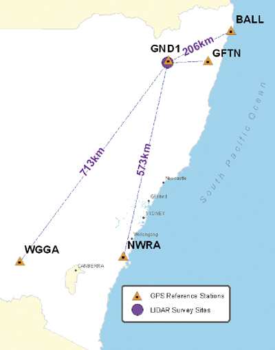
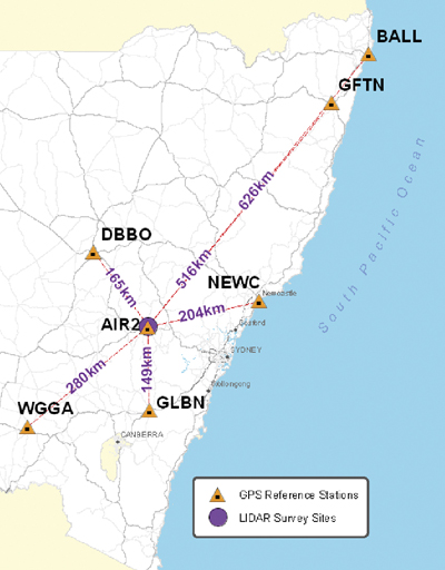
Glen Innes Test. This operational LiDAR survey established GND1 as the local reference station within the survey area. CORSnet-NSW data were collected for the test from GNSS receivers in Ballina (BALL), Grafton (GFTN), Nowra (NWRA), and Wagga Wagga (WGGA). FIGURE 2 shows the distribution of the reference stations and the flight runs.
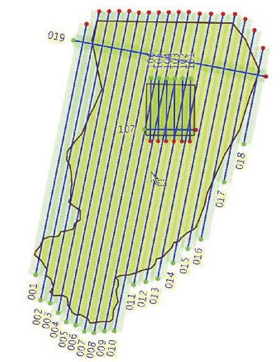
Figure 2. Glen Innes survey of June 9, 2009, showing the distribution of reference stations with baseline lengths and the survey area with (numbered) flight runs.Bathurst Test. Bathurst Airport is LPMA’s LiDAR calibration site and has various arrays of accurate ground checkpoints. AIR2, near the runway of the Bathurst airport, is the locally established GNSS reference station. CORSnet-NSW data were collected for the test from receivers in Ballina (BALL), Dubbo (DBBO), Grafton (GFTN), Newcastle (NEWC), Nowra (NWRA), and Wagga Wagga (WGGA). FIGURE 3 shows reference-station distribution and a schematic of the flight runs.
Figure 3. Bathurst test of June 16, 2009, showing the distribution of reference stations with baseline lengths and the survey area with (numbered) flight runs.
Effect on LiDAR Data
Rather than simply comparing aircraft trajectories, this study aimed to determine what effect the use of wide-area GNSS positioning has on the actual LiDAR point data and associated elevation surfaces. In terms of the horizontal accuracy required for LiDAR surveys, initial tests showed that the differences between the horizontal positions of various trajectories was negligible; therefore, only the vertical component was considered in this analysis.
To quantify differences between LiDAR data generated from trajectories using various combinations of distant GNSS reference sites, we applied four types of analysis:
Comparison of trajectories — directly compare the locally computed trajectory (assumed to be truth) with each wide-area derived trajectory.
Relative LiDAR point comparison — compare the positions for a sample of LiDAR ground points derived from the locally computed trajectory with those derived from each wide-area derived trajectory.
DEM comparison — difference the raster surfaces derived from the locally computed trajectory and a wide-area derived trajectory to find the effect over a LiDAR run.
Absolute LiDAR ground control comparison — compare the LiDAR derived surface from various trajectories to the surveyed ground control (Bathurst Calibration test site only). This also involves vertically shifting the resulting surface so that its offset relative to the one used as control is zero, thus removing the effect of using different reference frames for the GNSS trajectories and the control surface.
Trajectory Comparison
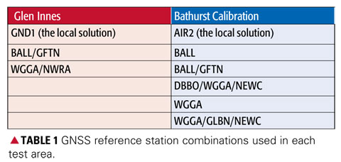
The comparison between the locally determined and each wide-area derived trajectory was made along the entire trajectory for each flight. The importance of this step lies in the assumption that all LiDAR data are directly positioned from the trajectory and so any systematic effect in the trajectory should be reflected on the ground. For each test site the locally derived solution is assumed to be “truth” with the vertical difference computed against wide-area solutions for each combination of reference stations used (TABLE 1).
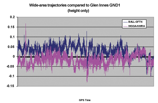
Glen Innes Test. FIGURE 4 shows the vertical comparison of two wide-area derived trajectories (using BALL and GFTN, and WGGA and NWRA, respectively) against the locally derived trajectory (using GND1). It can be seen that once the aircraft attained its stable operating altitude, the wide-area derived trajectories are generally within 5 centimeters of the locally derived solution.
Figure 4. Trajectory elevation differences for entire Glen Innes flight.
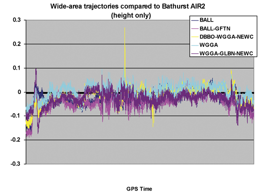
Bathurst Test. The Bathurst test differs from the Glen Innes test in that both the duration of the flight and the length of each run are significantly shorter. FIGURE 5 shows the vertical component of five wide-area derived trajectories, using several combinations of CORSnet-NSW reference stations, compared against the locally derived trajectory (using AIR2). The results once again show a remarkably consistent comparison with the locally derived solution. Data spikes showing up in the DBBO/WGGA/NEWC (yellow) solution were attributed to small data glitches at the DBBO CORSnet-NSW site. Unfortunately, LiDAR data were not collected at those instances; therefore, the effect on ground data could not be fully assessed.
Figure 5. Trajectory elevation differences for entire Bathurst calibration flight.
Relative Comparison
Regardless of the trajectory and orientation used to georeference LiDAR data, the same number of points will be created. It is therefore possible to create a LiDAR dataset using the same raw LiDAR data but different GNSS trajectories, and compare the results to determine the relative positioning differences on the ground.
Given the large number (many millions) of points in a LiDAR dataset, we used a representative sample of evenly spaced 10 2 10 meter areas each containing 50–100 points (on level ground) for statistical analysis. We calculated displacement vectors between points computed from the locally derived trajectory and those using wide-area trajectories. Results from flight run 002 at Glen Innes (see Figure 2) and run 7 at the Bathurst Calibration test site (see Figure 3) are presented here.
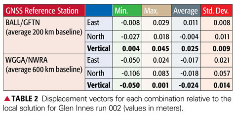
Glen Innes Test Run 002. The displacement vectors from 46 sample areas (4,620 points) are summarized in TABLE 2, being points computed using the two wide-area solutions compared with the locally derived solution using reference station GND1. Note the high accuracy achieved in the all important vertical component.
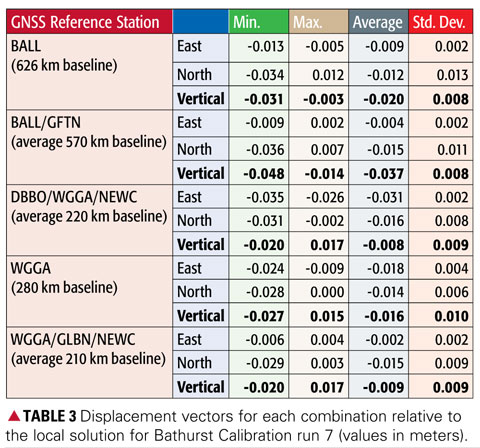
Bathurst Test Run 7. The displacement vectors from 25 sample areas (1,700 points) are summarized in TABLE 3, being points computed using the five wide-area solutions compared with the locally derived solution using reference station AIR2. Once again the results clearly show that the height values agree to within a few centimeters, even over baselines of more than 600 kilometers in length.
DEM Comparison
To investigate how the LiDAR surfaces derived from each trajectory compare across the entire data swath, we created raster surfaces from the LiDAR point data. Each surface was then subtracted from the local solution to create a difference surface. Visual inspection and interpretation was then used to discern any patterns or effects.
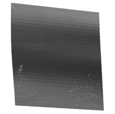
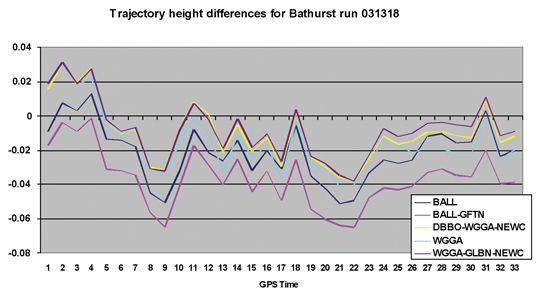
The result shown in FIGURE 6 (Bathurst Calibration flight run 7) was typical of the cyclical effect evident for all solutions. The magnitude of the difference was in the order of 2–3 centimeters and is in the direction of flight (north to south). If this cyclical variation is compared with the trajectory comparison for just the 33-second duration of flight run 7, a clear (expected) correlation with the variation in height is evident (FIGURE 7).
Figure 6. Subtraction surface for Bathurst Calibration run 7 (AIR2 vs. BALL).Figure 7. Trajectory comparison for Bathurst Calibration run 7 (031318).
No DEM comparison results are presented for the Glen Innes data because of significant variation in terrain and vegetation, making interpolation difficult and unreliable.
Absolute LiDAR Comparison
Ground control points serve two purposes in a LiDAR survey:
The calculation of statistics to describe vertical accuracy, that is, quantifying the match of the surface to the local height datum.
The calculation of a surface adjustment to enable transformation of the LiDAR points to fit the local height datum.
Additionally, ground control points with accurate heights are used to calibrate the sensor before use in active LiDAR surveys to account for internal electrical delays in the ranging and measurement system. LPMA maintains a calibration site at Bathurst Airport for this purpose, and regularly surveys the area to ensure the sensor is operating at maximum accuracy. It should be noted that the sensor was calibrated using Bathurst Airport ground control data prior to this study.
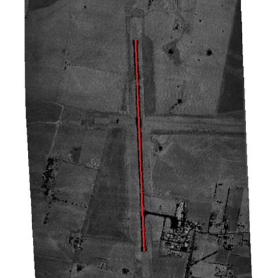
Surveyed Ground Control. The airport runway centerline vertical profile for the Bathurst Calibration site (FIGURE 8) was re-computed in terms of the same IGS05 reference frame determined for the LiDAR trajectories, thereby allowing an independent comparison with ground truth.
Figure 8. Runway vertical profile at the Bathurst Airport calibration site.
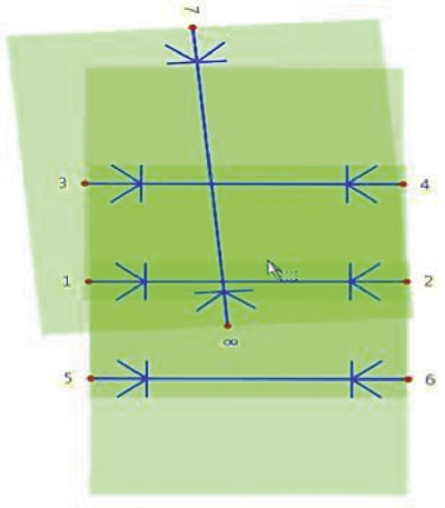
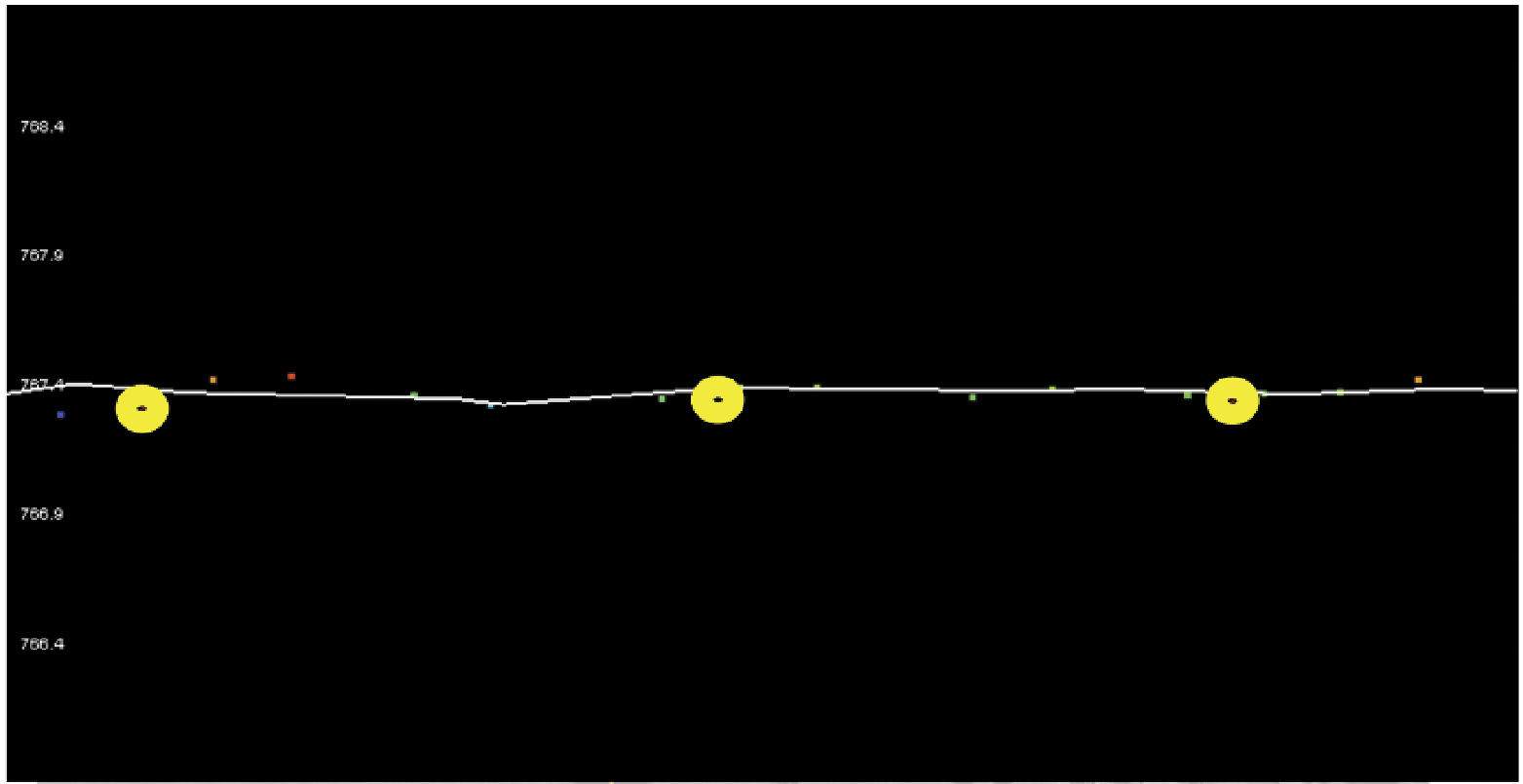
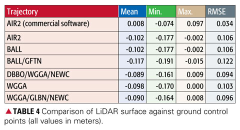
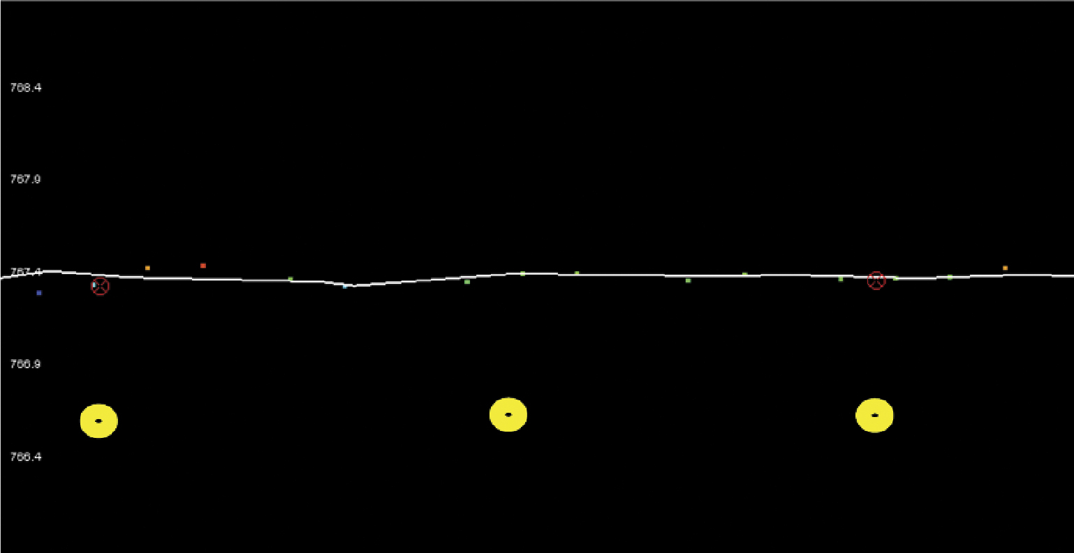
Point Comparison. Data from Bathurst run 7 were used to compare LiDAR results with the established ground control using a basic triangulated irregular network (TIN) surface comparison (FIGURE 9 and TABLE 4). In Figure 9, the TIN surface is indicated by the white line, while the ground control points are shown with yellow buffers.
Figure 9. Comparison of LiDAR surface and ground control points.
The first trajectory in Table 4 is the original calibration comparison using commercial software and orthometric height data. All wide-area solutions display a similar vertical offset, because of the use of different reference frames for the GrafNav and wide-area solutions (IGS05 vs. GDA94), and differences in the implementation in software of, for example, antenna corrections and atmospheric modeling. At first glance, the significant differences to the GrafNav trajectory caused the wide-area result to not satisfy the accuracy specifications for LiDAR. However, had the wide-area solutions been used for the sensor calibration, the figures would have been much closer to the ground truth.
Block-Shifted Data Comparison. In an operational environment, because of systematic errors in the resulting DEM relative to the local height datum, this mean vertical offset is a common occurrence with comparisons against ground control similar to those shown in FIGURE 10. Again, the TIN surface is indicated by the white line, and the ground control points are shown with yellow buffers.
Figure 10. Usual operational comparison of LiDAR surface and ground control points.
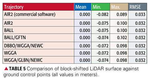
In standard LiDAR operations, the mean vertical offset between the initial results and the ground control, at the control points, produces a zero-mean offset. Following this procedure in this case results in the variation in the comparison of LiDAR data with ground truth now being well within the required limits of 615 centimeters (TABLE 5). The values show that after a block shift, trajectory solutions are virtually identical with a root mean square error of 32 millimeters. Thus, local GNSS reference stations can be replaced by distant CORS sites without loss of accuracy.
Conclusions
A precise wide-area positioning technique for airborne trajectory solutions provides both relative and absolute accuracies similar to those derived from usinga local GNSS reference station. Irrespective of which reference sites are used and once calibration and antenna modeling issues are addressed, the absolute comparison with ground control is well within the required accuracies. With the configuration of a GNSS network such as CORSnet-NSW (when complete, at least one site will always be within 150 kilometers of any point within New South Wales), an airborne LiDAR survey in the network’s service area can provide data for computation of an accurate sensor trajectory. This potentially negates the need to place and maintain ground reference stations close to the survey area — an exercise which not only requires significant resources but also reduces the operational flexibility of the aircraft.
The challenge for this technique in an operational environment is to define and maintain a precise reference frame for all CORSnet-NSW sites and observations, including the use of a stable ellipsoidal height datum with compatible geoid modeling in order to provide local orthometric elevation data. The knowledge base required for computation of wide-area GNSS solutions is significant and requires understanding of geodesy, GNSS positioning, absolute antenna modeling, application of precise ephemerides, and derivation of the other parameters inherent to successful ambiguity resolution over long distances.
Regardless of processing method, a LiDAR survey will always require independent ground surveys for collection of vertical checkpoints, which provide quality control to ensure the accuracy meets specifications, and the means to define any transformations necessary to fit LiDAR data with local height datum.
Manufacturer
NovAtel’s WayPoint GrafNav software was used for comparison purposes.
The ”IT” Software
Runs under Windows, Unix, Linux, and FreeBSD.
Source code compatible with most Fortran compilers.
Follows the IERS 2003 conventions.
Available mainly for collaborative research purposes, with a Free Software Foundation General Public Lice
nse.
Stop-and-go for rapid mobile surveys with pre-surveyed waypoints.
Differential, precise point positioning, mixed mode (precise differential + point positioning).
Data corrected for: Earth tide, neutral atmosphere radio signal delays, carrier phase windup, and so on.
Estimated parameters:
Receiver position in the IGS05 reference frame, with the WGS84 reference ellipsoid, earth spin-rate, light speed, GM constant.
Biases in ionosphere-free carrier-phase linear combination (“floated” ambiguities).
Neutral zenith delay correction error.
Broadcast orbit errors (allows precise differential near-real time solutions).
Integer ambiguity resolution available in differential mode, with short baselines up to 20 kilometers (in minutes), and baselines of unlimited length (in tens of minutes — or just minutes, with a precise ionosphere correction).
Oscar L. Colombo received a degree in electrical engineering from the National University of la Plata, Argentina, and a Ph.D. in electrical engineering from the University of New South Wales, Australia. He is an independent consultant.
Shane Brunker is an airborne LiDAR and imaging specialist working in a consulting capacity for specialized LiDAR survey company Network Mapping (United Kingdom).
Glenn Jones is a senior surveyor at the NSW Land and Property Management Authority in Bathurst, Australia.
Volker Janssen is a GNSS surveyor (CORS Network) in the Survey Infrastructure and Geodesy branch at the NSW Land and Property Management Authority in Bathurst, Australia. He holds a Ph.D. from the University of New South Wales.
Chris Rizos is head of the School of Surveying and Spatial Information Systems of the University of New South Wales, has a surveyor’s degree and a Ph.D. from the same university, and is an specialist in geodesy and GNSS positioning.
By Chaminda Basnayake, Tom Williams, Paul Alves, and Gérard Lachapelle
Communication-enabled vehicle safety has the potential to change transportation’s future, particularly vehicle-to-vehicle (V2V) and vehicle-to-infrastructure (V2I), collectively represented as V2X. An automakers’ consortium conducted extensive field trials to determine GNSS service availability and accuracy for the V2X challenge.
V2X can include applications based on communications between any two or more entities on the road. Of all the potential V2X applications, V2V applications probably lead the way in terms of maturity of prototype development and test efforts. General Motors (GM) demonstrated the first working prototype V2V system in 2005. Information on further industry collaborative efforts in V2V system developments can be found at the U.S. Department of Transportation’s (DOT’s) IntelliDrive website. While a multitude of applications could be developed based on V2I capability, most of the related system prototype development efforts have taken place under the DOT’s Cooperative Intersection Collision Avoidance (CICAS) program.
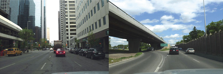
Driving environments encountered in testing. Clockwise from top left: deep urban, urban thruway, local roads, mountains.
Accuracy Requirements
In terms of positioning accuracy requirements, Vehicle Safety Communications-Applications (VSC-A) prototype system capabilities as well as all V2X applications can be classified as:
Which Road. In this case, accuracy is only required to the extent of identifying the road traveled. For instance, if a vehicle is in a service road parallel to a freeway, knowing that it is on the service road and not on the freeway is sufficient. The need of a typical vehicle navigation device is another good example of this requirement category. The typical accuracy requirement for this case is better than 5 meters. However, this could be a relative accuracy requirement for certain applications. For instance, in a V2V scenario, one vehicle may only need to know if the other is on the same road or not, while in the absolute sense both vehicles could be in error by more than 5 meters. For V2I applications, however, this becomes an absolute accuracy requirement, as the infrastructure is always mapped and identified with respect to a global coordinate frame.
Which Lane. This accuracy level enables applications to identify other entities with lane level resolution. The typical requirement is 1.5 meters or better, which approximately corresponds to half of a lane width. A blind-spot advisor is a good example that requires this accuracy.
Where-in-Lane. This accuracy level enables the relative positioning of entities to better than 1 meter. Further refinements of blind-spot advisor-like applications are examples.
Availability Requirements
GNSS as a line-of-sight technology has obvious limitations in certain environments, and these limitations are well understood by the GNSS community. The focus of this study was to understand the limitations associated with a GNSS-only V2X solution such that requirements for augmentation technologies can be defined. Therefore, no availability requirements were set for the system; estimating availability of a GNSS-only solution was the goal.
Why So Complicated? At first glance, what needs to be done is straightforward; all V2X-capable entities need to be aware of each other’s positions. Hence, if all entities transmit their own location with respect to the same coordinate system, the problem is solved. Unfortunately, it’s not that simple.
Designing the system so that hundreds of entities, potentially using all sorts of GNSS software and hardware, can work together presents a significant challenge. This includes keeping backward compatibility way out into the future.
Even within the same receiver make and type, inclusion of a particular satellite in the solution of one vehicle can significantly affect the solution difference between vehicles. Inclusion of SBAS also contributes as a differentiator. In a V2X scenario, out of two adjacent vehicles, one vehicle may use SBAS while the other may not, due to hardware configuration or visibility. If none of the above situations occurred and everything else were ideal, transmitting just the current horizontal position of a V2X entity over-the-air (OTA) would be sufficient to do everything needed.
V2X thus requires a positioning system architecture that minimizes the impact of these complications and many other potential compatibility issues. Major system design considerations include:
Performance Requirements. The system must provide relative positioning accuracy that fits Which Road, Which Lane, or Where-in-Lane category and should identify the solution quality. For instance, a vehicle on a freeway with relatively open sky view may function in the Which Lane mode and may transition to Which Road mode as it enters an urban area with sky visibility limitations.
Deployment Constraints. The system must be affordable for automotive applications. This may also include considerations such as antenna placement, processing resource requirements, and power requirements.
Bandwidth Constraints. The volume of data transmission constitutes a major consideration for OTA communications. While some methods manage communication range and frequency as a way of optimally using the communication channels, keeping the OTA data volume to a minimum by design was a goal.
Study Goals
This study investigated the performance of two relative positioning methods: DPOS, a method of using the difference in position reported by two entities to calculate the 3D separation between the points; and real-time kinematic (RTK). While there are many other possible relative positioning methods, these two were selected as they collectively represent the most desirable availability and accuracy performance. In DPOS, vehicle coordinates are transmitted between vehicles in order for position differences between vehicles to be derived at each vehicle. In RTK, raw code and carrier-phase data is transmitted between vehicles, and the inter-vehicle position differences are calculated using RTK software in either fixed or float carrier-phase ambiguity mode at each vehicle. The RTK method is more intensive both from a data transmission and computational aspect, but retains only common satellites in the solution, eliminating the problem described earlier. Its use of carrier-phase measurements also makes it more accurate.
The study included two GPS receiver types. The first, a single-frequency L1 automotive-grade receiver, is identified as Type B receiver in this study. The second, identified as Type A, was of a higher quality with proprietary multipath mitigation technologies. Both receivers were capable of using WAAS support. Receiver B also allowed the user to reject selected satellites from its solution. These two devices were selected as they were capable of supporting both processing methods, and represent on the one hand an existing automotive-grade receiver, and on the other hand one that is expected to be a good representation of a product with technologies available for automotive deployment a few years from now.
Specific study goals were:
Accuracy performance of DPOS and RTK methods when all vehicles use same GPS receiver type.
Same when a receiver type or a receiver configuration mix is used.
Dependency of the accuracy performance on the driving environment.
Solution availability with same receiver and mix receiver combinations.
Implications of non-continuous V2I coverage.
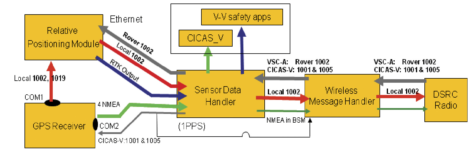
Prototype System
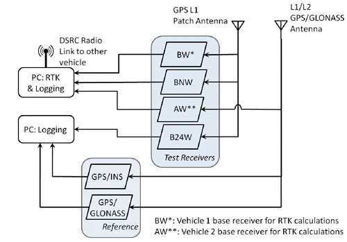
The system prototype (Figure 1) used for the study was a replica of the prototype relative positioning system implemented in the VSC-A project. It consists of a dedicated short-range communicatin (DSRC) interface with a DSRC radio, a GPS receiver/relative positioning module, and a sensor data handler.
In operation, a vehicle generates its own location information and GPS raw data in RTCM format and shares this data with other vehicles. OTA messaging was done using the SAE J2735 messages set with GPS raw data in RTCM format attached as optional data. As shown in Figure 1, RTCM v3 1002 messages were used to exchange VSC-A data. The system was also capable of using RTCM v3 messages 1001 & 1005 for V2I operation. The DPOS relative positioning logic was implemented in the sensor data handler, while the RTK implementation was done in a separate relative positioning module. This module takes in local and remote 1002 messages and outputs RTK data to the sensor data handler. Applications could access both RTK and DPOS relative positioning information from the sensor data handler.
Vehicle Setup. Two vehicles were used for the V2X data collection. Four different GPS L1-only test receiver types were installed on each vehicle:
AW: high-quality receiver using WAAS corrections.
BW: high-sensitivity automotive-grade receiver with WAAS ranging and corrections enabled.
BNW: high-sensitivity automotive-grade receiver with WAAS ranging and corrections disabled.
B24W: high-sensitivity automotive-grade receiver using a maximum of the four primary satellites in each of the six planes (minimum guaranteed constellation) and with WAAS ranging and corrections enabled.
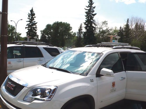
As shown in Figure 2, the AW and B type receivers were connected to different GNSS antennas. These antennas were mounted on roof-racks attached to the vehicles (see Photo). The patch antenna for the Type B receivers was mounted on an aluminum-topped wooden pedestal to bring it to approximately the same height as that used by the AW receivers, to provide a ground plane and to prevent shading from other equipment on the roof-racks. The spacing between the antennas was accounted for in all analysis.
Figure 2. High-level V2V hardware setup on each of the two test vehicles.
Figure 2 also shows that only three of the four test receivers, AW, BW, and BNW, were connected to the computer that ran the RTK software. This computer calculated the inter-vehicle vector (IVV) using information exchanged over the DSRC radio link in real time. The vehicles each had a designated base relative to which the IVV was calculated; for Vehicle 1 it was BW and for Vehicle 2 it was AW. Thus the computer on each vehicle calculated three instances of the IVV, for example, the computer on Vehicle 1 calculated BW1–BW2, BW1–BNW2, and BW1–AW2 (where Ri denotes the receiver of type R on vehicle i).
Transmission and reception of data between the two vehicles required for the IVV RTK calculations were achieved using wave radio modules with two magnetically mounted 802.11p antennas on each vehicle for redundancy. During testing, Vehicle 1 generally followed Vehicle 2. To minimize potential interference of roof-mounted instruments on between-vehicle communications, the antennas on Vehicle 1 were located close to the front of the roof, while those on Vehicle 2 were located close to the rear of the roof. In each case, 15 centimeters of roof space were left to provide ground planes for the antennas.
We used the single-point navigation solutions logged from each test receiver to calculate the IVV for each receiver combination using the DPOS method in post-processing. No real-time data transfer between the vehicles was used for this method.
Reference values of the IVV were calculated in post-processing using both geodetic grade GPS/GLONASS L1/L2 receivers and GPS/INS integrated systems in differential mode. Both were connected to the antenna used by the AW receiver. Differential GPS calculations were enabled by using stationary receivers with antennas at precisely known WGS84 locations on top of a building at the University of Calgary.
Two study vehicles with antennas attached to the roof-racks.
Test Scenarios
V2V data was collected in and around the city of Calgary in August 2009. In the majority of the tests, Vehicle 1 followed Vehicle 2 with a separation of less than 300 meters, the stated effective range of the DSRC link. For most tests the inter-vehicle separation was between 30 and 150 meters. Some driving environments forced modifications of the default behavior; for example, on highways, vehicles moved in between the two test vehicles, necessitating lane changes. Approximately 52 hours of data was collected over 12 days. After rejecting data due to various faults such as reference-system malfunction, more than 45 hours of data remained.
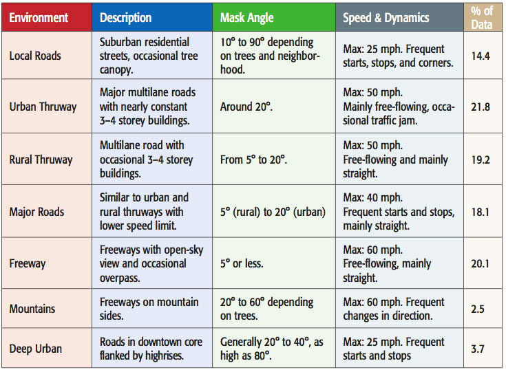
Data was collected in the seven test environments listed in Table 1. These environments were selected in accordance with Federal Highway Administration descriptions. Each environment provided different challenges for GNSS-based positioning. Obviously the deep urban environment was challenging because the reduced number of visible satellites and the large amount of multipath meant that navigation solutions were both rare and of poor quality. As another example, the mountain environment was interesting because often almost half the sky was occluded by trees on the mountain side, leading to an asymmetrical visible GPS satellite constellation with the associated solution degradation. The photos at the beginning of this article show selected driving environments encountered during testing.
Table 1. Description of driving environments used in V2V tests.
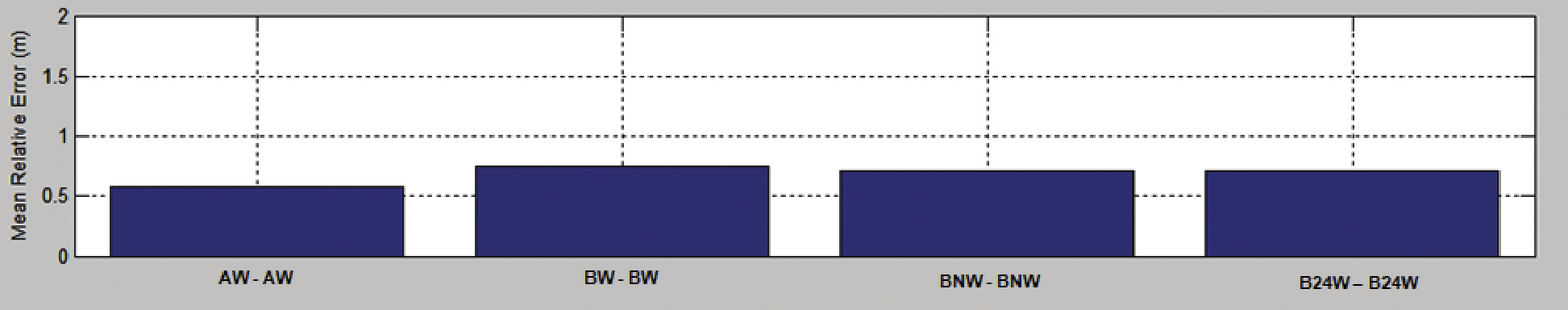
V2V Solution Accuracy. Positioning accuracy of the individual receiver was first investigated to estimate the V2V relative positioning accuracy when using the DPOS method. This was done for the entire dataset.
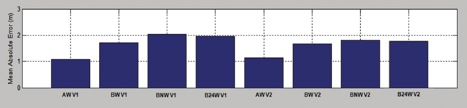
Figure 3A shows a representative freeway dataset to illustrate overall trends: the absolute 2D mean position errors observed from all eight GPS receivers used in both vehicles. The first set of four receivers shown were the AW, BW, BNW, B24W receivers in the first vehicle (V1), and the second set of receivers were the same type in the second vehicle (V2). As a general trend, Type A receivers provided better absolute accuracy meeting the Which Lane accuracy, whereas the Type B receivers provided Which Road accuracy. Also, the use of WAAS with receiver Type B has yielded some absolute accuracy improvement. Limiting the constellation to 24 (B24W) did not significantly degrade accuracy in this case.
As a second step, V2V relative accuracy when the same receiver type was used was estimated, and the mean errors are shown in Figure 3B. Based on the mean error for each pair, all four receiver pairs were able to provide Where-in-Lane relative position accuracy. The geodetic grade Type A receiver pair (AW–AW) yields the best relative accuracy at around 0.5 meters relative 2D error. In comparison with the mean absolute errors, the V2V relative accuracy is greatly improved as a result of cancellation of correlated errors, indicating a high degree of correlation of absolute errors in receivers under these test conditions.
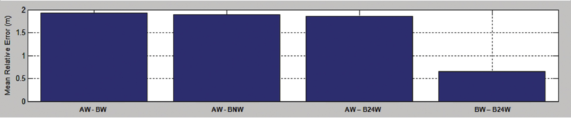
The relative accuracy with mixed receiver types or configurations was also estimated. With r
espect to receiver type mixes, the Type A receiver from vehicle 1 was used with the three Type B receivers in vehicle 2, yielding three combinations as AW–BW, AW–BNW, and AW–B24W. Mean error statistics for these three combinations and the combination of BW from vehicle 1 and B24W from the second vehicle are shown in Figure 3C. In comparison to the same type receiver pairing, this shows much larger mean errors. For instance, for all AW receiver mixes, the mean relative error is around 2 meters. Therefore, it is fair to conclude that error characteristics and modeling in the navigation solutions in receiver A and B are type-dependent, and they may not be compatible when a receiver mix is used. The BW–B24W combination does not show a significant increased mean error, indicating that the constellation difference in this test was not significant enough to result in an increased relative positioning error.
Figure 3A. Individual receiver absolute accuracy.Figure 3B. Relative accuracy with same receiver type.Figure 3C. Relative accuracy with receiver/configuration mix.
V2V Solution Availability
Availability statistics were generated for all accuracy categories (Which Road, Which Lane). At a more abstract level, solution availability statistics were also calculated for the DPOS and RTK methods. RTK solutions were defined as available whenever the software yielded a solution for that particular epoch. Data gaps in the RTK method could be caused by either communication failure due to, for example, a large truck entering the line of sight between vehicles, or one vehicle disappearing around a corner, or because insufficient observations from common satellites were available at the two vehicles. DPOS solutions, calculated in post-processing, were defined to be available whenever both receivers had observations from four or more satellites and were therefore able to calculate the necessary independent position solutions. While the two definitions of availability are not quite congruous, because only that for the RTK includes the possibility of communication failure, comparison of logs of data transmitted between the vehicles showed that out of approximately 45 hours of data, only 0.22 percent of missing RTK solutions could be attributed to failure of the DSRC link.
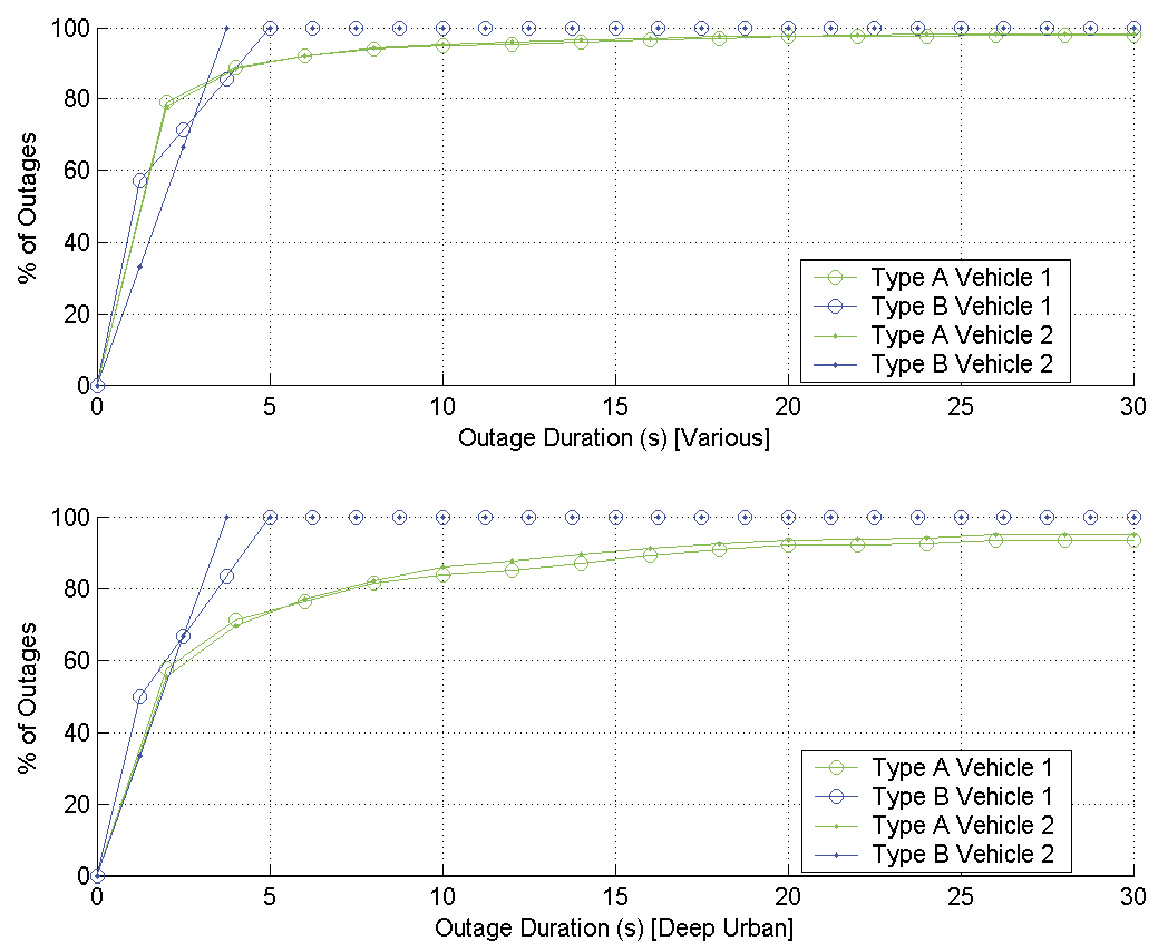
Figure 4 plots the distribution of GPS service outages observed by AW and BW receivers in individual vehicles in all of the test environments including deep urban. Here, as described for the DPOS method, an outage for a single receiver is identified on an epoch basis whenever the receiver has observations from less than four satellites. The total driving time included in this dataset is 45 hours and 4 minutes for each receiver. Figure 4 [deep urban] shows the same statistics for deep urban environment driving only, and this contains 1 hour and 40 minutes of driving for each receiver. The latter was selected specifically as this environment contained the most challenging conditions.
Figure 4. Distribution of GPS service outages for individual vehicles.
An important conclusion based on this data is that more than 98 percent of the individual vehicle-level service outages in the entire study lasted less than 30 seconds using any one of the receiver types. For the deep urban environment, 93 percent of the outages lasted less than 30 seconds. However, when using the high-sensitivity enabled Type B receivers, 100 percent of the outages lasted less than 5 seconds. No significant outage difference is seen between the observations from the same receiver type in the two vehicles.
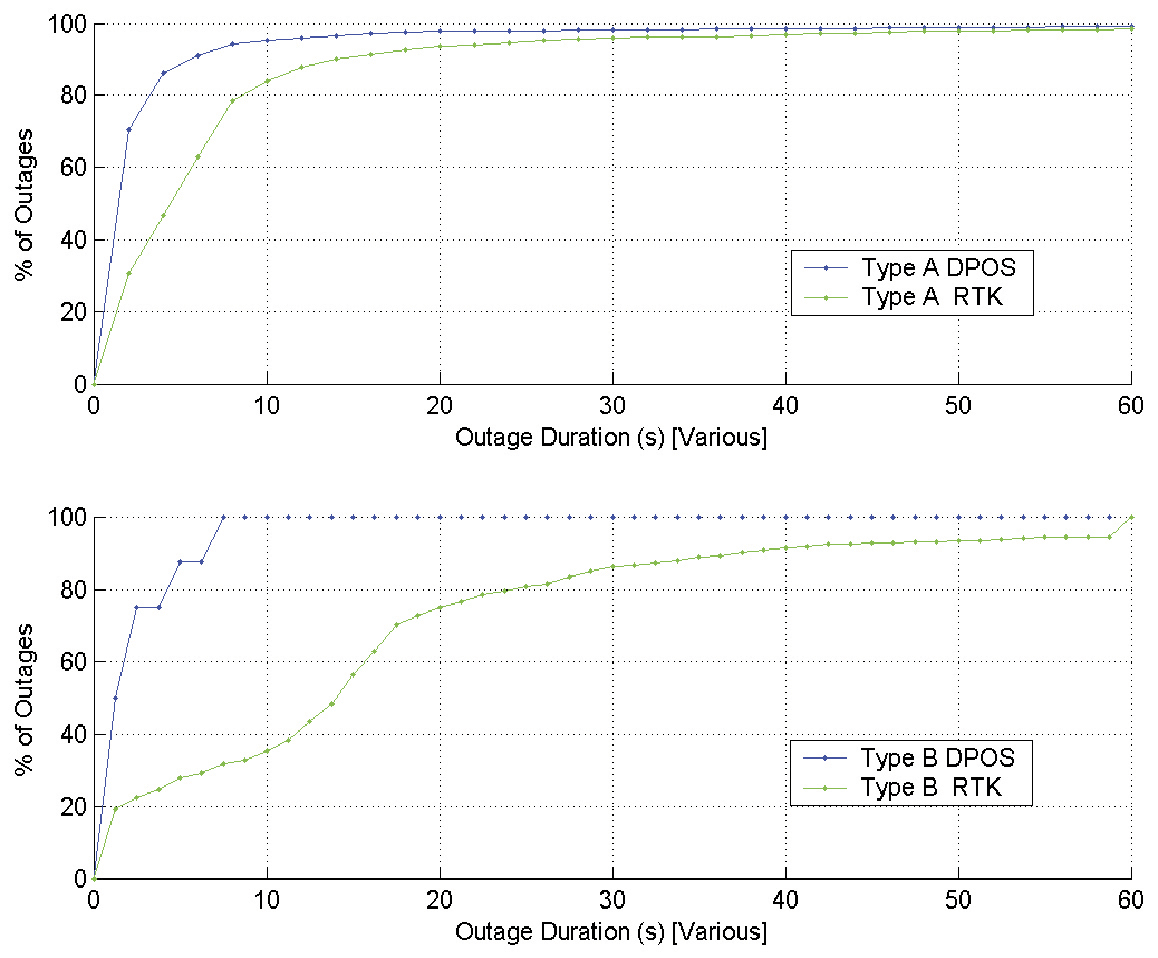
GPS service availability for V2V applications was calculated using two approaches for the two relative positioning methods. For the DPOS method, individual vehicle service availabilities were time-synchronized in post-mission, and V2V DPOS solution availability was estimated. Figure 5 compares V2V solution outages using both receiver types and both relative positioning methods.
Figure 5. Distribution of GPS service outages for V2V applications.
The DPOS method yields better solution availability statistics than RTK. With both receiver types, more than 95 percent of DPOS solution outages are less than 10 seconds. With the RTK method, relatively longer outages were observed, especially for Type B receivers. With Type A receivers, the difference is only significant for outages shorter than 30 seconds. For Type B receivers, larger percentages of longer RTK outages were observed; this can be potentially attributed to poor carrier-phase tracking loop performance of these receivers and the impact on RTK.
Using GNSS Data
We anticipated performance issues arising from receiver type and configuration incompatibilities going into the prototype development effort. We identified use of raw GPS measurements instead of the DPOS method as one method to overcome this limitation, as the differencing techniques with measurement data guarantees correlated error cancellation. This was one reason to include the RTK capability in the prototype system. Therefore, confirming the fact that use of raw measurements eliminates the receiver type and configuration-related incompatibilities was a major goal of the study.
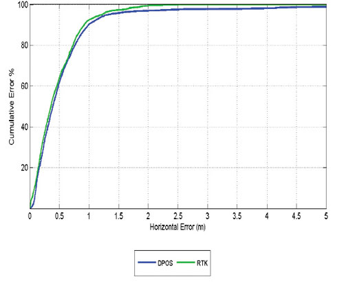
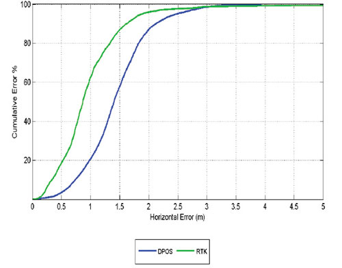
As discussed earlier, V2V relative position solutions using RTK were logged in real time as a part of the test setup. We compared these real-time RTK solutions and the DPOS solutions estimated in post-mission for all datasets. Figure 6 shows three cumulative probability distribution (CDF) plots generated using RTK and DPOS accuracy data from a freeway test dataset. The first CDF plot (left) shows the comparison of accuracy when both vehicles use Type A receivers with RTK and DPOS methods. The second CDF plot (center) shows the same CDFs when both vehicles use the Type B receivers. The third shows the DPOS and RTK accuracy CDFs when vehicle 1 uses Type A receiver and the other uses Type B receiver.
Figure 6 demonstrates that if higher quality GPS receivers similar to Type A are used in both vehicles, both RTK and DPOS methods would provide a solution of better than Which Lane accuracy more than 90 percent of the time. However, if Type B receivers are used, a solution with similar accuracy will only be available 60 percent of the time if the DPOS method is used for relative positioning of the vehicles. If the RTK method is used, this availability can be increased up to 90 percent.
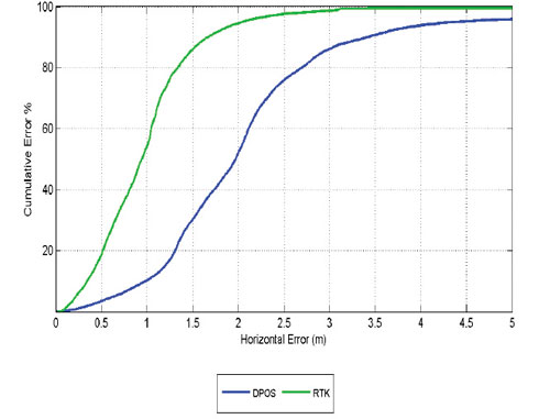
The performance difference between the two methods becomes even more prominent when the two vehicles use a mix of receiver types. In the right-most CDF of Figure 6, a solution with Which Lane accuracy is only available 30 percent of the time if DPOS method is used with the mixed receiver configuration. The RTK solution availability still remains around 90 percent even with the mixed configuration. This confirms that use of measurement data eliminates some of the limitations associated with the DPOS method.
Comparison of only the RTK performance between all three CDFs in Figure 6 shows that RTK V2V performance is only limited by the worst-performing receiver in the receiver combination. Out of the three CDFs, the middle (both vehicles using Type B) and the right (Type A and B mix) CDFs have almost identical RTK performance curves. Given that the RTK curve with both using Type A receivers shows much better performance, it is fair to conclude that in the mixed-receiver case, the RTK curve is limited by the performance of th
e Type B receiver. Figure 6 also shows that at Which Road accuracy, all receiver combinations and both processing methods yield almost identical performance.
Figure 6A. Comparison of V2V solutions using RTK and DPOS methods.Figure 6B. Comparison of V2V solutions using RTK and DPOS methods.Figure 6C. Comparison of V2V solutions using RTK and DPOS methods.
Other Approaches
Given that carrier-phase measurements are subject to cycle slips in some road environments, we ran a test using code measurements only in relative mode, using selected data sets collected on a mountainous highway. Only common satellites were used. Given that code measurements are not affected by a loss of phase lock, such a solution is more robust, but is subject to code noise and multipath. The RMS horizontal position differences between these solutions and the reference inter-vehicle separations were 25 centimeters and 1 meter for receiver Types A and B, respectively. Both receiver types meet the Where-in-Lane requirement in this test. Type A, with its low code noise and excellent code multipath-reduction capability, has a clear advantage.
Such an approach would represent a compromise between the DPOS and RTK approaches. Its advantage over the RTK approach is a lower data transmission-rate requirement, while that over the DPOS approach is the use of common satellites only. The latter is quite significant, since low-elevation satellites contribute the most to horizontal position solutions, but their measurements are affected more by atmospheric transmission errors that are most effectively removed in differential mode on a satellite-by-satellite basis.
V2V Operation with V2I
While infrastructure support can almost always improve the performance of other V2X applications, it can pose a challenge for positioning when such coverage is not continuous. The complication arises as a result of vehicles transitioning in and out of V2I coverage areas. V2I systems are highly likely to include GNSS augmentation capability so that vehicles within a coverage area benefit from better positioning capability. However, when vehicles transition from standard (V2V) operation mode to a V2I enhanced mode, some effects in the vehicle position domain can pose potential challenges for DPOS-based V2V.
The field study included test scenarios with limited V2I coverage in different driving environments: all of those described above with the exceptions of deep urban and mountains. In deployment, the infrastructure points (IPs) would broadcast aiding information to the vehicles within their coverage area, allowing real-time calculations. In the field study, in which the role of the IP was filled by a stationary high-grade receiver with a tripod-mounted antenna, all V2I estimates of the IVV were calculated using post-processing. Further, V2I estimates of the IVV were only calculated when at least one of the vehicles was within the coverage area of the IP, here chosen to be a circle of radius 300 meters centered at the IP. This range was chosen since it is the nominal effective range of the DSRC link.
The location of the IP, that is, the phase center of the stationary antenna, was determined using commercial RTK network software with additional stations at precise locations on the rooftop of a building at the University of Calgary. The estimated accuracy of this position was 5 millimeters (1 sigma). The distances of the vehicles from the IP, used to indicate when the vehicles transitioned into and out of the IP coverage area, were determined using the GPS/INS reference trajectories. In post-processing, once a vehicle was identified as having entered the IP coverage area, commercial RTK software was used to estimate the position of the vehicle, using the IP as base and each of the test receivers on that vehicle as rovers. The IVV was then calculated using the difference of the positions of the two vehicles. Thus, the V2I estimate of the IVV was determined using what is essentially the DPOS method with stationary base RTK-indicated vehicular positions, instead of the less accurate single-point GPS position solutions. When only one vehicle was within the coverage area, single-point solutions were used for the distal vehicle, resulting in a solution called V2I-S.
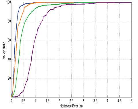
Figure 7 shows two sets of CDFs generated to illustrate the V2V positioning accuracy with V2I capability. The left plot corresponds to AW–AW receiver combination, and the right plot corresponds to the BW–BW combination. Each plot includes four curves. One pair of curves shows the V2V positioning accuracy without V2I, which includes performance when using the DPOS method (green) and another when using RTK (blue). The second pair shows the accuracy of the V2I and V2I-S estimates.
The most striking observation from Figure 7 is the separation of the V2I-S case from others for both receiver combinations (purple). It shows much worse positioning accuracy compared to the other three curves. For instance, using a BW–BW pair, the system will meet the Which Lane accuracy requirement around 80 percent of the time for either DPOS or RTK V2V without V2I support. However, when V2I coverage is available to only one vehicle, the V2I-S case, the accuracy requirement is only met at 40 percent confidence.
Figure 7A. Average relative positioning accuracy as a function of V2I positioning modes (orange V2I; green DPOS; blue RTK; purple V2I-S).Figure 7B. Average relative positioning accuracy as a function of V2I positioning modes (orange V2I; green DPOS; blue RTK; purple V2I-S).
Thus, system accuracy performance degrades when vehicles are operating in DPOS mode and are transitioning in and out of the V2I zones. This is because the V2I-S estimate is the difference of an accurate position solution for the vehicle within the coverage zone, and a potentially inaccurate single-point solution for the one outside the coverage zone. The beneficial cancellation of similar errors that occurs for DPOS estimates (using similar receivers and with common satellite observations) does not occur for V2I-S.
Potential solutions to this problem include using a V2I method of IVV calculation that is not dependent on the estimated position alone (that is, use RTK or other measurement-based methods as opposed to DPOS), or using a position-mode indicator with the DPOS mode such that a DPOS-based V2V solution is only generated when both vehicles are operating in the same mode (that is, V2I). However, the latter does not provide a remedy for the complications when the two vehicles are operating in two different modes. One could also consider a variation of the latter method whereby a V2I-augmented position and a non-augmented position is maintained by each vehicle, such that one of them could be used to generated a mode-matched DPOS V2V solution for a given sender.
Recommendations
These extensive trials provided valuable data demonstrating technical challenges associated with V2X positioning.
Error characteristics and modeling in the navigation solutions in receivers A and B are type-dependent, and they may not be compatible when a receiver mix is used with the DPOS mode. This is very likely to be the case for many other commercial receivers. Therefore, it is important to develop receiver hardware and software minimum-performance standards that define acceptable performance for measurement quality, satellite tracking and selection criteria, reliability estimates, navigation-solution parameters, and other such indicators.
Findings with RTK confirm the fact that use of measurement data eliminates some of the limitations associated with the DPOS method. While RTK is the most demanding raw data-based method in terms of processin
g requirements and OTA data needs, the study also conducted limited investigation on other methods that use raw code data and are less resource-intensive, and at the same time better performing than DPOS. Such an approach would represent a compromise between the DPOS and RTK approaches.
An important conclusion based on this data is that more than 98 percent of the individual vehicle-level service outages in the entire study lasted less than 30 seconds using any one of the receiver types. For the deep urban environment, 93 percent of the outages were less than 30 seconds. These statistics are useful for future research on suitable GNSS augmentation methods.
System accuracy performance degrades when vehicles operate in DPOS mode and transition in and out of the V2I zones. Potential solutions should be incorporated into the systems to take care of these limitations.
Acknowledgments
The authors thank the Crash Avoidance Metrics Partnership Vehicle Safety Communications-Applications team, in particular the Vehicle Positioning Technology Development team, for input. This work was conducted as a part of a CAMP VSC-A project under a cooperative agreement with the U.S. DOT.
CHAMINDA BASNYAKE is a senior research engineer at General Motors Global Research and Development and GNSS technology expert for GM OnStar. He leads GNSS-based vehicle navigation technology R&D efforts at GM and holds a Ph.D. in geomatics engineering from the University of Calgary.
TOM WILLIAMS is a postdoctoral researcher in the PLAN group in the Department of Geomatics Engineering at the University of Calgary.
PAUL ALVES is a Calgary-based geomatics consultant specializing in RTK. He obtained his doctorate from the University of Calgary.
GERARD LACHAPELLE holds an iCORE/CRC Chair in Wireless Location and heads the PLAN Group in the Department of Geomatics Engineering at the University of Calgary.
Global Positioning System experts from Air Force Space Command and the Space and Missile Systems Center will hold a media roundtable teleconference tomorrow, September 24, at 2:30 p.m. Mountain Time (4:30 p.m. Eastern Time) to discuss the recent GAO report titled “Global Positioning System: Challenges in Sustaining and Upgrading Capabilities Persist.” Colonel David Buckman, AFSPC command lead for positioning, navigation and timing, and Colonel Bernard Gruber, commander of the Global Positioning System Wing at Los Angeles Air Force Base, will participate in the teleconference.
Air Force Space Command, which has responsibility for sustaining and maintaining the Global Positioning System, feels that the GAO report is overly pessimistic and doesn’t adequately acknowledge what AFSPC has done to address constellation sustainment, according to a press release issued from the Air Force, Peterson Air Force Base, Colorado. “The Air Force has created the largest, most accurate constellation, with the greatest capability, in the history of GPS, with 31 operational satellites currently on orbit,” stated the press release. “This is well above the 24 minimum satellites needed for a full constellation and to meet constellation performance standards. Since 1995, GPS has never failed to exceed performance standards.”
The release continued, “AFSPC is working to mitigate the challenges identified by the GAO through a number of activities, including: applying a ‘back-to-basics’ approach to acquisition, continuing to identify additional ways to maximize the life of our operational satellites, implementing robust mission assurance processes, and transforming our launch enterprise.”
The first GPS IIF satellite completed on-orbit testing and checkout and was set operational on August 26 as planned, the Air Force said, The GPS IIF program is ready for full rate production and continues to build confidence in its production line. Through the institution of robust mission assurance processes, AFSPC is confident in the future of the GPS IIF program.
The follow-on program, GPS IIIA, recently completed critical design review, two months ahead of schedule, the Air Force said. “AFSPC is optimistic that its ‘back-to-basics’ approach, including stable requirements, mature technologies, and more government oversight, will ensure a successful program, providing the GPS IIIA and its ground segment, OCX, within a timeframe that maintains a robust GPS constellation and supports GPS users.”
The first time I ever heard of the Magnavox Research Laboratory in Torrance, California, was in 1966, as a young engineer working at Hughes Aircraft. We were building large (46-foot diameter) ground stations for the Defense Satellite Communications System (DSCS). Magnavox was supplying the secret anti-jam modems used in the terminals.
Because of this, I also learned a little about spread-spectrum pseudo-noise (PN), something quite esoteric at the time and not taught in engineering school. I noticed a widespread respect for Magnavox from my colleagues who referred to the company and its equipment as “Magicbox.”
Within a year I had transferred to the Hughes division responsible for developing satellites. We were working on a study known as 621B, for using satellites for positioning. Our teammate for the study was Magnavox. That team was responsible for the payload signal design, for which the team chose PN as the modulation to provide for multiple access, ranging, data transmission, and anti-jam.
Before long, my boss decided to leave Hughes and go work for Magnavox. He took two of his systems engineers with him. I was one of them.
In1968, the U.S. Air Force could not yet sell the 621B concept as an Advanced Development Program, so instead opted to experiment and prove that PN modulation could be used to accurately measure a half-mile of cable. Hughes bowed out since there wasn’t any satellite procurement in the offing. Magnavox and the other 621B contractor, TRW, each took on the challenge of measuring the cable.
Where Hughes had been 10-deep in Ph.D.s in every discipline, Magnavox was 10-deep in PN experts, which I believe at that time was the world’s majority. Thus it was natural for the Air Force to ask them to continue, and develop a receiver to be used in the next phase of 621B. An inverted range was set up with four PN transmitters, and an aircraft with the receiver and a bottom antenna flew over them. The aircraft’s position was determined using the PN range measurements and the known locations of the transmitters. The data from that receiver, called the MX450, was used to help justify the Department of Defense (DoD) decision to proceed into the Advanced Development Phase of GPS. Some of the people who contributed to this were named in Dr. Brad Parkinson’s recent articles on the origins of GPS. During that time I was working on the next generation of spread-spectrum modems for the DSCS.
Magnavox went on to develop these PN satcom modems for all three services, and thus was a natural choice to develop the first military GPS receivers (known as X and Y sets and the first Manpack), as well as the first C/A receiver, the Z set, and the very first spaceborne receiver called GPSPAC.
As soon as we completed the first Manpack, I approached Col. Paul Weber, the Joint Program Office Army Deputy Program Manger, and asked if he would pose with the Manpack on his back for a brochure we wanted to produce to show to potential Army and Marine Corps users. He agreed, dressed in his combat uniform, and went with our photographer into the wild woods of San Pedro (near the Port of Los Angeles) for the picture shown in the brochure.
Magnavox also developed the military GPS Engineering Models in competition with Rockwell Collins. Magnavox lost the production contract to Rockwell Collins a year after I left to join IEC, now known as L-3 Communications.
Magnavox also pioneered commercial GPS sets for use in the marine and survey markets. Today, you will still find many of the original GPS user equipment developers still at it as consultants and engineers at Raytheon, Navcom, Trimble, IEC, and others. Perhaps our most famous alumni is Dr. Min Kao, the “min” of Garmin.
Len Jaconbson
LEN JACOBSON is a consultant to the GPS industry and has served as an expert witness in many legal proceedings involving GPS. He is the author of the book GNSS Markets and Applications, published in 2007, and is a longstanding member of this magazine’s Editorial Advisory Board.
Earlier today (August 31), I conducted a webinar entitled “Solar Activity, SBAS and 24+3 GPS Constellation Updates.” Considering we only announced the webinar three weeks ago, we had a fantastic registration numbers, with more than 570 registered. Thank you for attending if you did. If you weren’t able to you’ll be able to download the presentation by registering here. After registering, you’ll be notified when it’s available for download (usually a couple of days after the webinar).
I had a lot of questions before and during the webinar. As customary, I’d like to address some of those as well as present the poll results here. First, the poll questions and results with accompanying pie charts to illustrate the results.
Poll #1: How concerned are you about solar activity affecting your GNSS operations?
Total votes: 157
Gakstatter comment: These numbers don’t surprise me. Personally, I probably fall in the “Somewhat” category, but my GPS/GNSS field work is pretty flexible so I can easily adjust without much inconvenience. However, if I had several crews using GPS/GNSS on a daily or near-daily basis or I had equipment relying on GPS/GNSS, I think I’d be in the “Very” category because the $$ impact would be much higher.
Poll #2: If it was available, would you be interested in receiving alerts/warnings of solar activity that may affect GNSS operations?
Total votes: 176
Gakstatter comment: I’m not surprised at these results either. When I initially considered this poll, I was thinking about asking which type of platform you would prefer to receive alerts/warnings with the choices being Droid app, iPhone app, Blackberry app, text message, e-mail, etc. If you have a preference on that, fire off a quick e-mail to me. Secondly, a few of you pointed out that NASA has an app for this, but keep in mind that the system I’m considering is focused specifically on high-performance/precision GPS/GNSS users, which would eliminate a lot of the baggage of the alert/warning systems available today. Poll #3: Do any of your GPS receivers use SBAS (WAAS/EGNOS/MSAS) as a primary source of corrections?
Total votes: 115
Gakstatter comment: Not much to say here except that a substantial number of commercial GPS users are relying on SBAS. This has definitely been the trend over the past five years.
Poll #4: Do you expect that the GPS 24+3 configuration will improve your GPS productivity?
Total votes: 172
Gakstatter comment: Like most of you, I have great expectations for the 24+3 configuration. While launching more satellites with L5 would be nice, that’s a long-term effort, whereas the 24+3 configuration is something we will benefit from in a few months and are seeing some marginal benefit now. In January 2011, once all the satellites have arrived at their destination slots, I’ll plot new visibility charts and see where we stand.
Following are some of the questions that were posed by the audience during the webinar: Question #1: The blueline ends in late 2009. Any information on up-to-date activity?
Gakstatter comment: This question was in reference to the Solar Cycle 24 prediction chart I displayed. The chart was probably small and difficult to read when displayed on your computer. Here’s a larger version of it. This was a chart released by the NOAA Space Weather Prediction Center in May 2009. Although sunspots don’t directly affect GPS operations, there is some relationship between sunspots and geomagnetic storms. Below it is an updated chart with actual values through the end of July 2010.
Question #2: What tools/online sites can be used to see if there is a TEC anomaly at a specified time, including “today”?
Gakstatter comment: There is a cool real-time chart of the U.S. on NOAA’s Space Weather Prediction Center website. There are other interesting charts on SWPC’s website like the 10-day trend chart. The JPL had a website that displayed a real-time TEC, but I just checked it and it hasn’t been updated since June. Another website to check is the National Satellite Test Bed that displays a real-time plot of the WAAS ionospheric grid points. Click here to view a global real-time (updated every 60 minutes) TEC chart of the world published by the Australian Space Weather Agency.
Question #3: What is better for a receiver, Differential GPS or dual frequency? Any references on this?
Gakstatter comment: With respect to performance during periods of heightened solar activity, definitely dual-frequency receivers. Although I don’t have a specific cite for you right now, there has been plenty written on this subject. Single frequency DGPS receivers are the most vulnerable during periods of heightened solar activity.
Question #4: Is the disruption in the sub-meter scale, single-digit meters, or tens of meters?
Gakstatter comment: It depends on the severity of the geomagnetic storm. During the worst times of the Oct. 2003 event, it was up to 25 meters. That order of magnitude would be rare. Remember, those events occurred in about four days over the 11-year cycle. I have some figures that relate TEC to position error, but I’ll withhold those until I’ve got a better understanding of how practical they are.
Question #5: Is there some type of notification system for GNSS users of major solar events? E-mail alerts? Twitter tweets?
Gakstatter comment: Following are instructions for signing up for the NOAA alerts/warnings. This is a good start. Stay tuned for my alert/warning system later this fall. Follow me on Twitter at http://twitter.com/GPSGIS_Eric
Following are detailed instructions for signing up for alerts:
-Click on Email products (under the Support Services menu on the left)
-Create an account if you don’t have one already (it’s free).
-Click on Subscribe
You don’t want to subscribe to everything. Here are the ones specific for GPS operations:
-Advisories/Space Weather Bulletin
-Geomagnetic Storm Products/(sign up for both Alerts and Warnings for K6, K7, K8, K9 events.
-For high latitude (55 degrees and higher) users, als
o sign up for Alerts and Warnings for K4 and K5 events.
Question #6: There is already an iPhone/iPod application that gives alerts of solar activity.
Gakstatter comment: Yes, I’m aware of the NASA app and there maybe others, but in my opinion they are too broad for high-performance/high-precision GPS/GNSS users. Personally, I don’t need to know about new sunspots and where they are located on the sun (although it’s cool to see in that app). I need to know when geomagnetic events are occurring that may interrupt or affect my GPS/GNSS fieldwork.
Question #7: Ouch, we’re at 59 degrees north, and 134 west. Seems like these problems are “picking” on Juneau.
Gakstatter comment: The good news for you is that Alaska has the most dense concentration of WAAS Reference Stations in the entire WAAS coverage area. Well, maybe not Juneau, but certainly “mainland” Alaska :-). Seriously, parts of Alaska produce the best WAAS accuracy due to the high density of WAAS reference stations.
Question #8: Will parts of BC, Canada, be affected by the SBAS outage?
Gakstatter comment: Not really, except that you’ll have one less WAAS GEO satellite in view for a month or so until PRN 133 is operational in November. I don’t think you’ll notice any change in performance. The exception would be if your receiver uses SBAS ranging. In that case, you’d be tracking one less satellite between the time that PRN 135 becomes unusable and the time PRN 133 becomes operational.
Following is an elevation plot of the current WAAS GEO satellites (PRN 135 and PRN 138):
Following is an elevation plot of only PRN 138. This is a possible scenario after PRN 135 is unusable in October 2010 and before PRN 133 is placed into service in November 2010.
Following is an elevation plot of PRN 138 and the new PRN 133 GEO which is expected to be placed into service sometime in November 2010.
Question #9: With the 24+3 configuration, is it that some sats were flying almost in tandem and they are spreading them out more?
Gakstatter comment: Yes, that is essentially what is happening. Some believe, including me, that a 24+6 configuration would be even better! But, one step at a time. I feel good that the U.S. Air Force is listening and responding.
I addressed many of the questions from the webinar. Some will take a little research on my side to answer properly. I should be able to address those in the mid-September newsletter. Thanks again to those who registered for the webinar. Feel free to send me an e-mail any time with comments, suggestions or questions.
You might have heard reports this week about a solar storm this week. This is part of the new solar cycle (Solar Cycle 24) that I’ve written about several times. I want to periodically touch on this subject as the solar activity is going to increase over the next few years, and if the solar activity (geomagnetic storms, not sunspots) is severe enough, it will have an effect on GPS accuracy and tracking. Here’s the scoop on this week’s solar activity.
First of all, I’ll let you in on a secret. I’m working on a new solar activity notification system specifically designed for GPS users. The problem is that people see reports in the mainstream media about solar activity and they automatically assume that it’s going to affect their GPS. Not all solar storms affect GPS; in fact only very specific ones (geomagnetic storms) of sufficient strength will affect GPS operations. I’m working on a notification system that will be tailored to both GPS L1 and GPS L1/L2 users (they are affected differently) so GPS users can have a reliable and specific source of information on solar activity without having to wade through the mainstream media noise.
Stay tuned for details this fall in this newsletter to learn more about my notification system and how to and access it. If you’ve ever used some of the GPS hardware/software products I helped design, you know my top priority is to make it easy to use and understandable.
This week’s event was probably the strongest geomagnetic storm of this solar cycle and of recent years (edit: actually, the storm in early April 2010 was a little stronger), maybe since late 2006. It will create some beautiful “northern lights,” but as strong as that may seem, it still wasn’t strong enough to elicit even a “cautionary” warning to GPS users (neither GPS L1 nor GPS L1/L2).
NASA video of sun’s activity on August 2, 2010
The last geomagnetic storm that adversely affected GPS users was in December 2006. It affected some GPS users for 10-15 minutes. For such a short time, most users would not notice or they might attribute it to a local system malfunction. By the time they investigate and reset the system, the event has passed and the user is back in operation. It was barely noticeable, if at all.
On the other hand, a severe geomagnetic storm such as the one that occurred in October 2003 can last for days and wreak havoc on precision GPS receivers. During extreme geomagnetic storms like that one, GPS accuracy suffers a lot, especially with GPS L1 users. During that event, simulations from the University of Calgary showed that WAAS maximum horizontal error (95th percentile) reached 25 meters while single baseline DGPS maximum horizontal error (95th percentile) reached 18 meters.
Dual-frequency users aren’t affected as much by extreme events but aren’t immune. Extreme events such as October 2003 can cause a loss of phase lock, especially with L2 on receivers that utilizing codeless and semicodeless techniques, which are virtually all of the dual-frequency GPS receivers on the market as of today.
For GPS users, nothing can be done to mitigate the effects of a strong geomagnetic storm. The next best step is to try to predict when they will occur so GPS users know what to expect. Fortunately, these storms are not common and scientists can reasonably predict when an event will occur.
There are some good websites to reference when checking up on solar activity. A great place for Europeans to do this is at the Royal Meteorological Institute of Belgium’s website. The U.S. National Weather Service also operates the Space Weather Prediction Center. The Australian Space Weather Agency operates a Space Weather Prediction Center, too. Also, note that for those users along the equator and at higher latitudes, your area is more susceptible to stronger geomagnetic storm activity.
The websites listed above are chock full of information and predictive systems on space weather. In fact, I believe it’s too much information for most GPS users to efficiently interpret. The goal with my new initiative is to provide GPS users with a quick summary so they are able to make informed decisions in a few seconds. Again, stay tuned this fall for the rollout.
Conference/Webinar Presentations
Between webinars and conferences, I’ve put together a fair number of Powerpoint presentations. I’m in the process of uploading many of them, some dating back years, to our website. Currently, I’ve uploaded ones that date back to April 2010. I hope you enjoy them.
The following presentations have all been converted to PDF format and are copyrighted. Feel free to incorporate them (or parts of them) into your documents if you like, just please remember to attribute each page you use to my name, Eric Gakstatter, and GPS World/Geospatial Solutions.
2010 (July San Diego, California) ESRI Surveying and Engineering GIS Summit luncheon keynote presentation: Get It Surveyed (GIS).
2010 (June, Seattle, Washington) Asia-Pacific Economic Cooperation meeting: Mapping and Surveying with SBAS+GPS.
2010 (June, Portland, Oregon) Webinar: GIS Mapping for Forestry, Agriculture, and Other Natural Resource Professionals.
Note that for the following webinar, you can also download an audio portion of the webinar free of charge by clicking here.
2010 (April, Phoenix, Arizona) GITA Annual Conference: How the Evolution of GPS is Transforming Surveying and Mapping (along with Pamela Fromhertz of NGS).
Part 1 – GNSS Mapping/Surveying Technology Update
2010 (April, Phoenix, Arizona) GITA Annual Conference: How the Evolution of GPS is Transforming Surveying and Mapping (along with Pamela Fromhertz of NGS).
Part 2 – Machine Control Using GNSS
2010 (April, Phoenix, Arizona) GITA Annual Conference: How the Evolution of GPS is Transforming Surveying and Mapping (along with Pamela Fromhertz of NGS).
Part 3 – Sub-Meter Mapping Using GPS
2010 (April, Phoenix, Arizona) GITA Annual Conference: How the Evolution of GPS is Transforming Surveying and Mapping (along with Pamela Fromhertz of NGS).
The field at Commonwealth Stadium in Edmonton, Alberta, recently received a CDN $2 million renovation. The old natural-grass field had become expensive to maintain properly, and the Grey Cup game, Canada’s Super Bowl, will be played at Commonwealth Stadium this year. The stage needed to be re-set.
Renovation required total removal of the existing medium and subgrade materials to a 1.2-meter depth. Wilco Contractors Northwest replaced the subgrade to a planarity or flatness tolerance of 3 millimeters over a 3-meter length. To achieve this precision, Wilco used a machine automation system on a Volvo G-960 motor grader fitted with a GPS receiver, and base station nearby. A second grader carried a robotic total station.
“We probably have a quarter-million dollars invested in this,” said Wilco President Art Maat. “The machine-control equipment pays for itself on an annual basis. It enables us to construct projects to tolerances that other contractors cannot match, even though they have the same big iron capabilities we do.”
Work began with removal of existing soil mixes, drainage rock, and subgrade clay. A bulldozer and the two motorgraders graded the subgrade to a 0.5 percent slope on both sides of the field’s center spine. The work included the D-shaped zone behind each goal post, created by a running track encircling the field. In all areas, the slope must be constant. “The problem is, how do you grade that half-circle?” said Maat. “Grader operators and surveyors want to work in straight lines or on rectangular grids. We use the geo-tracker, or robotic total station, to control the grader blade three-dimensionally. It is one step more accurate than a GPS system.”
Using the robotic total station involves entering a digital terrain model, called a TIN-file, into the grader’s onboard computer. The grader is fitted with a mast and prism, which has a fixed relation to the grader blade. The robotic total station can see the prism, read its 3D location, and communicate it back to the grader. The computer processes the differences between the actual blade location and the digital terrain model to control the blade.
The GPS-equipped grader did the rough grading at 20-millimeter accuracy, and the prism-equipped grader handled the fine grading at sub-centimeter accuracy. With final subgrade complete, Wilco dug trenches to install a drainage system, covered with a geotextile. Working in four lifts of 300 millimeters each, Wilco filled the excavation with coal bottom ash, a gritty product like playground sand. “We took the TIN file and offset the elevation by 300 millimeters at a time.”
Savings. The machine-control equipment saved Wilco $15,000–$20,000 on surveying, for 100 hours or more at $150 an hour for a crew. “The systems make our equipment 25 percent more efficient on low-tolerance sites such as fields and running tracks where grades are critical,” Maat added.
To test planarity, Wilco stretched a stringline over a 3-meter distance at many points on the field and measured with a Canadian dollar coin, a looney. If they could fit a couple of loonies under the string, they had found a low spot. If they could fit only one, the 3-millimeter tolerance had been met. “Our feedback from the consultants was that they had never seen a field prepared this well, with very little adjustment required. The slope of the field had to be 0.25 percent from the centerline spine to the sides. And the slope of the D-shaped areas behind the goal posts was exactly the same.”
Manufacturers
Wilco uses a Leica PowerGrade GPS/GNSS receiver, Leica Redline base station, Redline Power Tracker robotic total station, and Geo-Tracker.
INRIX announced it has expanded its European real-time traffic coverage to 18 countries making it the largest traffic network in Europe. With the launch of real-time traffic information in Ireland, Hungary, Poland and Slovenia since February, INRIX traffic services now cover more than 1 million kilometers of motorways, city streets and secondary roads, throughout Europe — more than 2X the amount of real-time road coverage of its nearest competitor.
“Whether driving across town or across borders, European customers uniquely benefit from INRIXs ability to reliably help drivers avoid traffic congestion wherever their travels take them,” said General Manager of INRIX Europe Dr. Hans-Hendrik Puvogel. “Through our expanded coverage, continuous technology innovation in support of standards like TPEG over IP, and growing customer base, we’re proving to the market everyday why we’re the best provider of quality traffic services across Europe.”
In a separate announcement today, INRIX introduced a breakthrough in the delivery of traffic information called TPEG Connect. Based on the new encoding and transmission standard for traffic and travel information developed by the Transport Protocol Experts Group (TPEG), INRIX TPEG Connect provides automakers and navigation application providers with the ability to optimize payloads and bandwidth for delivering richer real-time and predictive traffic flow, incident, and location-based services like weather conditions on the road to devices using TPEG over IP. By providing delta support that can reduce data payloads by up to 50 percent on each message request, INRIX TPEG Connect helps OEMs and consumers save on connectivity costs by reducing data consumption in ways that ensures only the most location-relevant real-time information is delivered to the device.
“TPEG Connect provides the industry with a better way to deliver pan-European traffic information that enables the delivery of more dynamic traffic and traveler information at less cost both to the OEM as well as the consumer,” said INRIX Vice President of Product Management Ken Kranseler, “By making the standard production for use over IP, INRIX TPEG Connect removes key technical and commercial hurdles for our customers accelerating the delivery of next generation of traffic applications and driver services that will improve mobility for millions of people worldwide.”
According to the announcement, INRIX delivers the broadest and most accurate real-time traffic information through its distinctive Smart Driver crowd-sourced traffic information network and Total Fusion data analytics technologies. The company offers real time traffic information today in the following European countries:
Austria
Belgium
Denmark
Finland
France
Germany
Hungary
Italy
Ireland
Luxembourg
The Netherlands
Norway
Poland
Spain
Sweden
Switzerland
Slovenia
United Kingdom
INRIX also announced an agreement with road safety products and services company Coyote Systems to provide real-time traffic information in future Coyote products. As Coyote’s preferred global provider of traffic information, INRIX and Coyote will work together to apply each other’s expertise in user-generated content for the development of future products and services.