Tag: Doppler

  • Modern Northstar: Starlink LEO PNT across land, air, stratosphere and Arctic Seas

    Modern Northstar: Starlink LEO PNT across land, air, stratosphere and Arctic Seas

    In January 2015, SpaceX publicly announced its plan to launch Starlink: a mega constellation of nearly 12,000 satellites in low-Earth orbit (LEO) to provide global broadband internet service. In May 2019, the first batch of 60 operational satellites were launched.

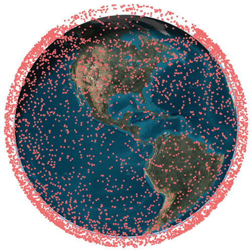
    In October 2025, Starlink surpassed 10,000 satellites (see Figure 1). This remarkable achievement means that Starlink has more satellites than all other constellations have ever launched into LEO combined.

    SpaceX is redefining global connectivity, delivering high-speed, low-latency internet anywhere on the planet1. Its civilian system, Starlink, is bridging the digital divide by providing reliable broadband in remote and underserved regions, enabling education, telemedicine and economic growth. Its defense and government variant, Starshield, is offering secure, resilient communications and rapid data transfer for military operations.

    Figure 1 The current constellation of Starlink satellites in LEO, as of January 2026.
    Figure 1 The current constellation of Starlink satellites in LEO, as of January 2026.

    In the midst of the COVID pandemic, in a quiet campus building, the ASPIN Laboratory was busy researching Starlink’s mysterious proprietary signals and the satellites’ poorly known orbits. Having demonstrated the first experimental unmanned aerial vehicle (UAV)2 and ground vehicle3 navigation using Orbcomm LEO satellites, the team’s next grand objective was to exploit Starlink’s signals of opportunity for positioning, navigation, and timing (PNT). At the 2021 ION GNSS+ Conference, the team announced a new era of LEO PNT: the first successful exploitation of Starlink for PNT4. The team designed a cognitive software-defined receiver (SDR) capable of tracking the carrier phase 5 and Doppler6 of Starlink’s so-called pilot tones along with ephemerides error correction algorithms7. The SDR and algorithms were put into test to localize a stationary receiver. Starting from an initial estimate nearly 180 km away, listening to six Starlink satellites resulted in localizing the receiver to within 10 m. This led to worldwide research to study Starlink for PNT, from deciphering Starlink’s downlink orthogonal frequency-division multiplexing (OFDM) signals8,9, to analyzing its ephemerides and timing10,11, to studying the achievable PNT performance12,13.

    This article presents the most advanced LEO PNT results to date with Starlink on four mobile platforms at geographically dispersed locations:

    1. Ground vehicle in Pennsylvania

    2. UAV in Ohio

    3. Extremely high-altitude balloon in New Mexico

    4. Maritime vessel in the Arctic near Greenland

    Exploiting Starlink LEO for PNT: The enablers

    SDR and signal analysis

    Unlike GNSS, non-cooperative LEO satellites such as Starlink do not publicly disclose the structure of their downlink signals, so users must build their own “LEO PNT Interface Control Document (ICD)14. This can be achieved via “reverse-engineering” the signal. A more powerful approach to “reverse-engineering” is via cognitive SDRs, which employ blind signal processing techniques to learn the signals on-the-fly, regardless of the adopted modulation and multiple-access scheme15.

    The most comprehensive characterization to date of Starlink’s downlink signals for PNT was unveiled in16, utilizing the cognitive SDR approach, in which:

    1. The full OFDM beacon was revealed.

    2. Theoretical and experimental description for exploiting Starlink for PNT was provided, showing the maximum achievable carrier-to-noise density ratio (C/N0) under different scenarios: (i) pilot tones versus OFDM-based beacons and (ii) low-gain versus high-gain reception captures.

    3. A Starlink LEO PNT SDR was designed, yielding the first successful extraction of navigation observables (carrier phase, Doppler shift and code phase) from Starlink’s OFDM signals.

    4. A detailed analysis of the quality of Starlink navigation observables, including (i) signal activity and power levels and (ii) timing corrections that contaminate extracted observables along with mitigation strategies.


    Ephemeris and timing error correction

    Unlike GNSS, non-cooperative LEO satellites, such as Starlink, do not broadcast ephemeris and clock data, so users rely on public sources, such as two-line element (TLE) files. However, this data degrades over time due to orbital perturbations, limiting their effectiveness for PNT. Recent research addressed this challenge through five main approaches:

    1. Differential LEO17,18

    2. Machine learning-based orbit prediction19,20

    3. Measurement error correction21,22

    4. Closed-loop ephemeris tracking23,24

    5. Equivalent timing error compensation25,26

    The next sections will showcase experimental LEO PNT results with Starlink signals of opportunity. All experiments utilized the SDR developed in16 and the ephemerides and timing correction methods developed in26-28.


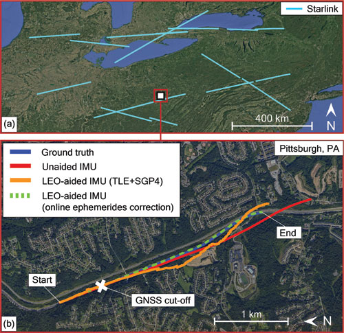
    Ground vehicle navigation in Pennsylvania

    The experiment was conducted in June 2025. The ground vehicle navigated for 3 km in 120 seconds on Interstate 79 by Pittsburgh, Pennsylvania. GNSS signals were available for the first 30 seconds but were virtually cut off for the last 90 seconds, during which the vehicle traversed a 2.25 km trajectory. The vehicle was equipped with a VectorNav VN-310 dual GNSS/INS operating with real-time kinematic (RTK) corrections and a tactical-grade inertial measurement unit (IMU), from which the vehicle’s ground truth was generated. Starlink signals were captured over all eight Ku-band downlink channels using an upward low-noise block with feed-horn (LNBF) and processed at 2.5 MSps via two NI X410 USRPs.

    Figure 2 shows the ground vehicle’s hardware setup.
    Figure 2 shows the ground vehicle’s hardware setup. shows the ground vehicle’s hardware setup.

    The vehicle navigated by fusing Doppler shift measurements from 11 Starlink satellites in a tightly-coupled fashion to aid the IMU, while altimeter measurements were fused in a loosely-coupled fashion. IMU updates were performed at a rate of 200 Hz. Starlink Doppler measurement updates were performed at a rate of 1 Hz with measurement noise variance inversely related to the received C/N0, ranging between 0.05 (m/s)2 and 6.5 (m/s)2, while altimeter updates were performed at a rate of 10 Hz with a measurement noise variance of 3 m2. The vehicle-mounted receiver and LEO satellites’ oscillator qualities were assumed to be that of an oven-controlled crystal oscillator (OCXO). A prior for the vehicle’s position and velocity was obtained from the on-board GNSS system. Starlink LEO satellites’ ephemeris errors were corrected via the equivalent timing error compensation technique in an online fashion as described in28. Each satellite’s equivalent timing error state was initialized with 0, while the relative clock drift state was initialized as the difference between the measured and predicted pseudorange rate.

    An extended Kalman filter (EKF) was used to estimate the state vector, consisting of the vehicle’s orientation, 3D position, 3D velocity and the IMU’s 3D gyroscope and accelerometer biases along with the relative clock drift error between the receiver and each LEO satellite. The Starlink satellites’ orbits were generated by propagating TLE files with SGP4 for the duration of the experiment. The navigation solution was generated using three approaches:

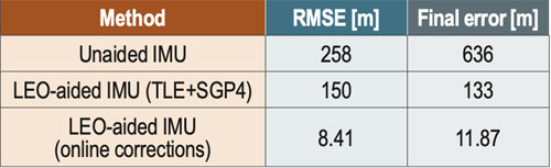
    1. Unaided IMU: The vehicle navigates via open-loop IMU measurements when GNSS measurements are unavailable.

    2. LEO-aided IMU with TLE+SGP4 ephemerides: The vehicle fuses LEO measurements with IMU and altimeter measurements while incorporating TLE+SGP4 ephemerides in the navigation filter.

    3. LEO-aided IMU with online ephemerides corrections: The vehicle fuses LEO measurements with IMU and altimeter measurements. Starting with TLE+SGP4 ephemerides, the navigation filter estimates an equivalent timing error for each satellite as described in28.

    Figure 3 shows the Starlink satellite trajectories, as well as the vehicle’s ground truth and estimated trajectories with the three navigation approaches. The unaided IMU solution drifted to a 3D position root mean squared error (RMSE) of 258 m from the truth trajectory. The LEO-aided IMU solution that incorporated the erroneous TLE+SGP4 ephemerides resulted in a 3D position RMSE of 150 m, while the navigation solution employing the online ephemeris correction method resulted in an RMSE of 8.41 m. Table 1 summarizes the navigation results.
    Figure 3 shows the Starlink satellite trajectories, as well as the vehicle’s ground truth and estimated trajectories with the three navigation approaches. The unaided IMU solution drifted to a 3D position root mean squared error (RMSE) of 258 m from the truth trajectory. The LEO-aided IMU solution that incorporated the erroneous TLE+SGP4 ephemerides resulted in a 3D position RMSE of 150 m, while the navigation solution employing the online ephemeris correction method resulted in an RMSE of 8.41 m.
    Table 1 summarizes the navigation results.
    Table 1 summarizes the navigation results.

    UAV navigation in Ohio

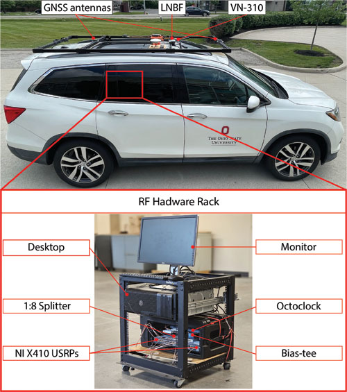
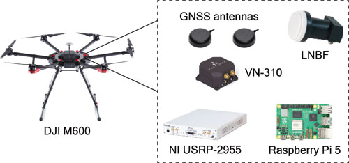
    The experiment was conducted in August 2025. A DJI M600 UAV navigated for 500 m in 75 seconds in Columbus, Ohio. GNSS signals were available for the first 20 seconds of the experiment but were virtually cut off for the last 55 seconds, during which the UAV traversed a 370 m trajectory. The UAV was equipped with a VectorNav VN-310 dual GNSS/INS operating with RTK corrections and a tactical-grade IMU, from which the UAV’s ground truth was generated. Starlink signals were captured from the 4 low-side Ku-band channels using an upward LNBF and processed at 2.5 MSps via an NI 2955 USRP. Figure 4 shows the UAV’s hardware setup.

    Figure 4 UAV’s hardware setup.
    Figure 4 UAV’s hardware setup.

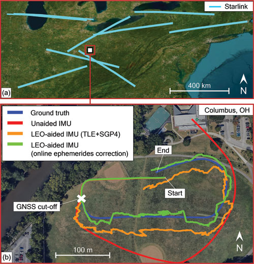
    The UAV navigated by fusing Doppler shift measurements from nine Starlink satellites in a tightly-coupled fashion to aid the IMU, while altimeter measurements were fused in a loosely-coupled fashion. IMU updates were performed at a rate of 200 Hz. Starlink Doppler measurement updates were performed at a rate of 1 Hz with measurement noise variance inversely related to the received C/N0, ranging between 0.09 (m/s)and 6.75 (m/s)2, while altimeter updates were performed at a rate of 10 Hz with a measurement noise variance of 3 m2. The UAV-mounted receiver and LEO satellites’ oscillator qualities were assumed to be that of an OCXO. A prior for the UAV position and velocity was obtained from the UAV’s on-board GNSS system. Starlink LEO satellites’ ephemeris errors were corrected via the equivalent timing error compensation technique in an online fashion as described in 28. Each satellite’s equivalent timing error state was initialized with 0, while the relative clock drift state was initialized as the difference between the measured and predicted pseudorange rate.

    An EKF was used to estimate the state vector, consisting of the UAV’s orientation, 3D position, 3D velocity and the IMU’s 3D gyroscope and accelerometer biases, along with the relative clock drift error between the receiver and each LEO satellite. The Starlink satellites’ orbits were generated by propagating TLE files with SGP4 for the duration of the experiment. The navigation solution was generated using the three approaches described in Section II.

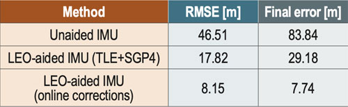
    Figure 5 shows the Starlink satellite trajectories, as well as the UAV’s ground truth and estimated trajectories with the three different navigation approaches. The unaided IMU solution drifted to a 3D position RMSE of 46.51 m from the truth trajectory. The LEO-aided IMU solution that incorporated the erroneous TLE+SGP4 ephemerides resulted in a 3D position RMSE of 17.82 m, while the navigation solution employing the online ephemeris correction method resulted in an RMSE of 8.15 m. Table 2 summarizes the navigation results.

    Figure 5 Experimental results of Doppler-based UAV navigation with Starlink: (a) trajectories of the nine Starlink satellites used to navigate the UAV and (b) UAV’s trajectory (blue) and estimated trajectories via the unaided IMU solution (red) and LEO-aided IMU solutions when incorporating the (i) uncorrected TLE+SGP4 ephemerides (orange) and (ii) online ephemeris correction (green).
    Figure 5 Experimental results of Doppler-based UAV navigation with Starlink: (a) trajectories of the nine Starlink satellites used to navigate the UAV and (b) UAV’s trajectory (blue) and estimated trajectories via the unaided IMU solution (red) and LEO-aided IMU solutions when incorporating the (i) uncorrected TLE+SGP4 ephemerides (orange) and (ii) online ephemeris correction (green).
    Table 2 Experimental results: UAV 3D position errors.
    Table 2 Experimental results: UAV 3D position errors.

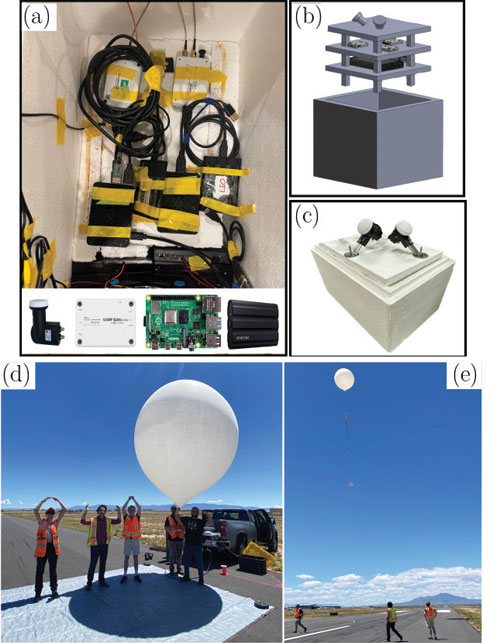
    High-altitude balloon navigation in New Mexico

    The experiment was conducted in July 202429. The balloon was launched from the Moriarty Municipal Airport in Moriarty, New Mexico, and landed just south of Mountainair, New Mexico, traveling a horizontal distance of about 105 km south with a 3D distance of about 119 km. The balloon reached a peak altitude of about 25.3 km (83,128 ft) above sea level. A specific time period was studied to evaluate utilization of Doppler observables for navigation at an elevation of 82,177 ft. During this period, five different Starlink satellites were tracked over a 50-second period, during which the balloon traveled 948 m.  The balloon was equipped with a VectorNav VN-200 GNSS/INS, from which the ground truth trajectory was generated. Starlink signals were captured over two Ku-band downlink channels using an upward LNBF and processed at 2.5 MSps via two Ettus B205-mini USRPs. Figure 6 shows the balloon’s hardware setup.

    Figure 6 (a)-(c) High-altitude balloon’s hardware setup. (d) OHIO in New Mexico, left to right: Jennifer Sanderson, Zak Kassas, Will Barrett and the Icarus Balloon. (e) Balloon launch.
    Figure 6 (a)-(c) High-altitude balloon’s hardware setup. (d) OHIO in New Mexico, left to right: Jennifer Sanderson, Zak Kassas, Will Barrett and the Icarus Balloon. (e) Balloon launch.

    The balloon navigated by fusing Doppler shift measurements from five Starlink satellites and altimeter measurements via an EKF. The dynamic model of the high-altitude balloon was chosen as a velocity random walk model, with acceleration process noise spectra set to 0.5 m2/s3 in the in the East, North and 0.8 m2/s3 in the in Up directions, respectively. Starlink Doppler measurement updates were performed at a rate of 10 Hz with measurement noise variance inversely related to the received C/N0, ranging between 1.40 (m/s)2 and 7.01 (m/s)2, while altimeter updates were performed at rate of 10 Hz with a measurement noise variance of 1 m2. The process noise covariance for the clock states was constructed according to an OCXO clock quality. A prior for the balloon’s position and velocity was obtained from the on-board GNSS system. Ephemeris data for each satellite was obtained from offline SGP4-propagated TLE, with epoch time corrections made by minimizing the residuals between predicted Doppler and measured Doppler26,27.

    The EKF state vector consisted of the balloon’s 3D position and 3D velocity along with the relative clock drift error between the receiver and each LEO satellite. The navigation solution was generated using (i) an open-loop approach, which simply propagated the states via the dynamical model and (ii) the LEO+altimeter approach.

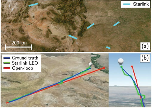
    Figure 7 shows the balloon’s ground truth and estimated trajectories with the two different navigation approaches. The open-loop solution drifted to a 3D position RMSE of 83.34 m from the truth trajectory, while the LEO-aided solution resulted in an RMSE of 12.28 m. Table 3 summarizes the navigation results.

    Figure 7 Experimental results of Doppler-based high-altitude balloon navigation with Starlink: (a) trajectories of five Starlink satellites used and (b) balloon’s trajectory (blue) and estimated trajectories via the open-loop solution (red) and LEO-aided solution (green).
    Figure 7 Experimental results of Doppler-based high-altitude balloon navigation with Starlink: (a) trajectories of five Starlink satellites used and (b) balloon’s trajectory (blue) and estimated trajectories via the open-loop solution (red) and LEO-aided solution (green).
    Table 3 Experimental results: High-altitude ballon 3D position errors.
    Table 3 Experimental results: High-altitude ballon 3D position errors.

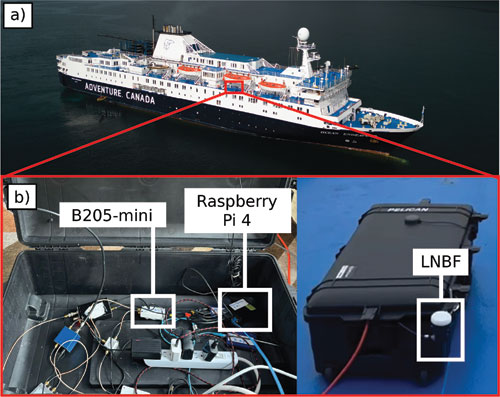
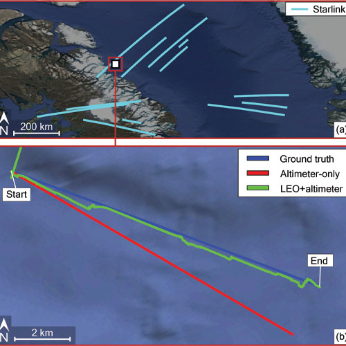
    Maritime navigation in the Arctic

    The experiment was conducted in August 202430. The vessel navigated for 8.5 km in 20 minutes off the shore of Baffin Island, Nunavut, Canada. Starlink signals were captured over the third Ku-band downlink channel using an upward LNBF and processed at 2.5 MSps via a B205-mini USRP and a Raspberry Pi 4. Figure 8 shows the vessel’s hardware setup.

    Figure 8 Vessel’s hardware setup.
    Figure 8 Vessel’s hardware setup.

    The vessel navigated by fusing Doppler shift measurements from 12 Starlink satellites and altimeter data via an EKF. The dynamic model of the vessel was chosen as a velocity random walk model. Starlink Doppler measurement and altimeter data updates were both performed at a rate of 10 Hz with measurement noise variances of 4.5 (m/s)2 and 3 m2, respectively. The vessel-mounted receiver and the LEO satellites’ oscillator qualities were assumed to be that of an OCXO. The vessel’s position states were initialized from the true position obtained from the on-board GNSS system. The velocity was initialized from the true velocity but with a 10˚ clockwise error with respect to the vessel’s direction-of-motion. The Starlink satellites’ orbits were generated by propagating TLE files with SGP4 for the duration of the experiment. Ephemeris errors were corrected by adjusting the TLE epoch time for eachsatellite26,27 to minimize the residuals between predicted Doppler and measured Doppler.

    An EKF was used to estimate the state vector, consisting of the vessel’s 3D position, 3D velocity and the relative clock drift errors between the receiver and each LEO satellite. The navigation solution was generated via two approaches: (i) using only altimeter data and (ii) using LEO Doppler fused with altimeter data.

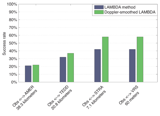
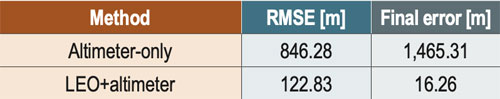
    Figure 9 shows the Starlink satellite trajectories, as well as the vessel’s ground truth and estimated trajectories with the two navigation approaches. The altimeter-only solution drifted to a 3D position RMSE of 846 m from the truth trajectory. The LEO+altimeter solution resulted in a 3D position RMSE of 123 m. Table 4 summarizes the navigation results.

    Figure 9 Experimental results of Doppler-based vessel navigation with Starlink: (a) trajectories of the 12 Starlink satellites used to navigate the vessel and (b) vessel’s true trajectory (blue) and estimated trajectories using (i) only an altimeter (red) and (ii) using LEO + altimeter (green).
    Figure 9 Experimental results of Doppler-based vessel navigation with Starlink: (a) trajectories of the 12 Starlink satellites used to navigate the vessel and (b) vessel’s true trajectory (blue) and estimated trajectories using (i) only an altimeter (red) and (ii) using LEO + altimeter (green).
    Table 4 Experimental results: Vessel 3D position errors.
    Table 4 Experimental results: Vessel 3D position errors.

    Acknowledgments

    This work was supported in part by the Office of Naval Research (ONR) under Grants N00014-22-1-2242 and N00014-22-1-2115, in part by the Air Force Office of Scientific Research (AFOSR) under Grant FA9550-22-1-0476, in part by the U.S. Department of Transportation under Grant 69A3552348327 for the CARMEN+ University Transportation Center, in part by The Aerospace Corporation under Award 4400000428, and in part by the Laboratory Directed Research and Development program at Sandia National Laboratories under award 2543953. Sandia National Laboratories is a multimission laboratory managed and operated by National Technology & Engineering Solutions of Sandia LLC, a wholly owned subsidiary of Honeywell International Inc., for the U.S. Department of Energy’s National Nuclear Security Administration under contract DENA0003525. This paper describes objective technical results and analysis. Any subjective views or opinions that might be expressed in the paper do not necessarily represent the views of the U.S. Department of Energy or the United States Government.

    The authors would like to thank Vasilios Konstantacos, Jackson Morris, Ethan Shaw, Khaled Hamil, Aiden Short and Andrew Ye for constructing the balloon’s payload; Mark Andrews for supervising the payload design; and Prabodh Jhaveri, Danny Bowman, Mike Fleigle and Justin LaPierre for helping with launch and recovery of the balloon. The authors would also like to thank The Explorers Club and Adventure Canada for their help with data collection in the Arcitc. The authors would like to thank VectorNav for supplying the VN-200.

    References

    1. A. Yadav, M. Agarwal, S. Agarwal, and S. Verma, “Internet from space anywhere and anytime – Starlink,” in Proceedings of International Conference on Advancement in Electronics & Communication Engineering, pp. 1-8, 2022.

    2. J. Morales, J. Khalife, A. Abdallah, C. Ardito, and Z. Kassas, “Inertial navigation system aiding with Orbcomm LEO satellite Doppler measurements,” in Proceedings of ION GNSS+ Conference, pp. 2718-2725, 2018.

    3. Z. Kassas, J. Morales, and J. Khalife, “New-age satellite-based navigation – STAN: simultaneous tracking and navigation with LEO satellite signals,” Inside GNSS Magazine, (14)4, pp. 56-65, 2019.

    4. M. Neinavaie, J. Khalife, and Z. Kassas, “Exploiting Starlink signals for navigation: first results,” in Proceedings of ION GNSS+ Conference, pp. 2766-2773, 2021.

    5. J. Khalife, M. Neinavaie, and Z. Kassas, “The first carrier phase tracking and positioning results with Starlink LEO satellite signals,” IEEE Transactions on Aerospace and Electronic Systems, (58)2, pp. 1487-1491, 2022.

    6. M. Neinavaie, J. Khalife, and Z. Kassas, “Acquisition, Doppler tracking, and positioning with Starlink LEO satellites: first results,” IEEE Transactions on Aerospace and Electronic Systems, (58)3, pp. 2606-2610, 2022.

    7. Z. Kassas, M. Neinavaie, J. Khalife, N. Khairallah, S. Kozhaya, J. Haidar-Ahmad, and Z. Shadram, “Enter LEO on the GNSS stage: navigation with Starlink satellites,” Inside GNSS Magazine, (16)6, pp. 42-51, 2021.

    8. T. Humphreys, P. Iannucci, Z. Komodromos, and A. Graff, “Signal structure of the Starlink Ku-band downlink,” IEEE Transactions on Aerospace and Electronic Systems, (59)5, pp. 6016-6030, 2023.

    9. M. Neinavaie and Z. Kassas, “Cognitive sensing and navigation with unknown OFDM signals with application to terrestrial 5G and Starlink LEO satellites,” IEEE Journal on Selected Areas in Communications, (42)1, pp. 146-160, 2024.

    10. S. Hayek and Z. Kassas, “Warm start navigation with non-cooperative LEO satellites via online ephemeris error estimation,” in Proceedings of IEEE/ION Position, Location, and Navigation Symposium, pp. 112-123, 2025.

    11. W. Qin, A. Graff, Z. Clements, Z. Komodromos, and T. Humphreys, “Timing properties of the Starlink Ku-band downlink,” IEEE Transactions on Aerospace and Electronic Systems, (62), pp. 727-744, 2026.

    12. H. More, E. Cianca, and M. De Sanctis, “Comparing positioning performance of LEO mega-constellations and GNSS in urban canyons,” IEEE Access, (12), pp. 24465-24482, 2024.

    13. Z. Kassas and J. Saroufim, “LEO PNT frameworks for non-cooperative satellites with poorly known ephemerides: open-loop SGP4, tracking, and differential,” IEEE Aerospace and Electronic Systems Magazine, (40)1, pp. 46-71, 2025.

    14. S. Kozhaya, H. Kanj, and Z. Kassas, “Multi-constellation blind beacon estimation, Doppler tracking, and opportunistic positioning with OneWeb, Starlink, Iridium NEXT, and Orbcomm LEO satellites,” in Proceedings of IEEE/ION Position, Location, and Navigation Symposium, pp. 1184-1195, 2023.

    15. S. Kozhaya, S. Hayek, and Z. Kassas, “Cognitive beacon estimation of unknown LEO satellites signals of opportunity for PNT,” IEEE Journal on Selected Areas in Communications, pp. 1-16, 2026, in-press.

    16. S. Kozhaya, J. Saroufim, and Z. Kassas, “Unveiling Starlink for PNT,” NAVIGATION, Journal of the Institute of Navigation, (72)1, pp. 1-35, 2026.

    17. J. Khalife and Z. Kassas, “Performance-driven design of carrier phase differential navigation frameworks with megaconstellation LEO satellites,” IEEE Transactions on Aerospace and Electronic Systems, (59)3, pp. 2947–2966, 2023.

    18. M. Hasan, M. Kabir, M. Islam, S. Han, and W. Shin, “A double difference Doppler shift-based positioning framework with ephemeris error correction of LEO satellites,” IEEE Systems Journal, (18)4, pp. 2157-2168, 2024.

    19. Z. Kassas, S. Hayek, and J. Haidar-Ahmad, “LEO satellite orbit prediction via closed-loop machine learning with application to opportunistic navigation,” IEEE Aerospace and Electronic Systems Magazine, (40)1, pp. 34-49, 2024.

    20. K. Selvan, A. Siemuri, F. Prol, P. Välisuo, and H. Kuusniemi, “Machine learning for LEO and MEO satellite Orbit prediction,” in Proceedings of ION GNSS+ Conference, pp. 3556 -3571, 2024.

    21. J. Saroufim and Z. Kassas, “Ephemeris and timing error disambiguation enabling precise LEO PNT,” IEEE Transactions on Aerospace and Electronic Systems, (61)3, pp. 6138–6153, 2025.

    22. J. Saroufim and Z. Kassas, “LEO ephemeris error modeling enabling long baseline correction for improved PNT,” in Proceedings of IEEE/ION Position, Location, and Navigation Symposium, pp. 625–630, 2025.

    23. N. Khairallah and Z. Kassas, “Ephemeris tracking and error propagation analysis of LEO satellites with application to opportunistic navigation,” IEEE Transactions on Aerospace and Electronic Systems, (60)2, pp. 1242–1259, 2024.

    24. S. Kozhaya, J. Saroufim, S. Hayek, P. El-Kouba, and Z. Kassas, “Light will guide you: passive joint DOA/FOA sensing, tracking, and navigation with unknown LEO satellites,” in Proceedings of IEEE/ION Position, Location, and Navigation Symposium, pp. 716–727, 2025.

    25. Y. Du, H. Qin, and C. Zhao, “LEO satellites/INS integrated positioning framework considering orbit errors based on FKF,” IEEE Transactions on Instrumentation and Measurement, (73), pp. 1-14, 2024.

    26. S. Hayek, J. Saroufim, and Z. Kassas, “Analysis and correction of LEO satellite propagation errors with application to navigation,” in Proceedings of ION GNSS+ Conference, pp. 1800 -1811, 2024.

    27. S. Hayek and Z. Kassas, “Modeling and compensation of timing and spatial ephemeris errors of non-cooperative LEO satellites with application to PNT,” IEEE Transactions on Aerospace and Electronic Systems, (61)3, pp. 5579-5593, 2025.

    28. S. Hayek and Z. Kassas, “A reduced-order model of simultaneous tracking and navigation with LEO satellites”, IEEE Aerospace and Electronic Systems Magazine, in preparation.

    29. W. Barrett, J. Sanderson, S. Kozhaya, J. Saroufim, and Z. Kassas, “Evaluation of Starlink LEO satellite signals for high-altitude platform station opportunistic navigation,” in IEEE International Conference on Wireless for Space and Extreme Environments, pp. 100-105, 2024.

    30. W. Barrett, S. Kozhaya, Z. Kassas, and D. Marsh, “Navigating the Arctic Circle with Starlink and OneWeb LEO satellites,” in Proceedings of IEEE Military Communications Conference, pp. 1–6, 2025.

    Authors

    Zaher (Zak) M. Kassas is the TRC Endowed Chair in Intelligent Transportation Systems and Professor of Electrical and Computer Engineering at The Ohio State University (OSU). He is also Director of the Autonomous Systems Perception, Intelligence, & Navigation (ASPIN) Laboratory and Director of the U.S. Department of Transportation Center for Automated Vehicles Research with Multimodal AssurEd Navigation (CARMEN).

    Samer Hayek is a Ph.D. student at OSU and member of the ASPIN Laboratory.

    Will Barrett was a member of the ASPIN Laboratory.

    Sharbel Kozhaya is a Senior Research Associate at the ASPIN Laboratory.

    Paul El-Kouba is a Ph.D. student at OSU and member of the ASPIN Laboratory.

    Faezeh Mooseli is a Ph.D. student at OSU and member of the ASPIN Laboratory.

    Jennifer Sanderson is a Ph.D. student at OSU and member of the ASPIN Laboratory. She is also an R&D Engineer with Sandia National Laboratories.

    Joe Saroufim is a Ph.D. student at OSU and member of the ASPIN Laboratory.

  • Low-cost antennas power high-precision space-based positioning

    Low-cost antennas power high-precision space-based positioning

    A novel method using signals of opportunity from low-Earth orbit (LEO) satellites is redefining what’s possible in satellite-based navigation. Researchers have developed a joint pseudo-range and Doppler positioning technique that taps into signals from constellations like Starlink and Iridium NEXT — without relying on traditional navigation signal structures.

    By employing low-cost, wide-beam antennas and a specially designed time–frequency inversion algorithm, the team achieved remarkable accuracy: 3.6 meters in 2D and 6.2 meters in 3D, surpassing Starlink positioning approaches based on parabolic antennas by 35%.

    Technical barriers in using signals of opportunity include signal transmission times, low signal power, and imprecise orbital data, all of which hinder accurate positioning. Addressing these challenges demands a new approach to extracting usable navigation data from LEO constellations.

    In response, researchers from the Aerospace Information Research Institute introduced a joint pseudo-range and Doppler positioning method using wide-beam antennas to receive LEO satellite SOPs. The approach centers on a signal time–frequency inversion algorithm that reconstructs key signal parameters, alongside a novel accuracy metric called Equivalent Position Dilution of Precision (EPDOP).

    Real-world experiments combining Starlink Doppler data and Iridium NEXT pseudo-range signals confirmed strong performance, especially in long-baseline conditions — reinforcing the method’s global applicability.

    To overcome the cost and complexity of existing satellite tracking equipment, the team employed low-noise bock (LNB) wide-beam antennas capable of simultaneously receiving signals from multiple Starlink satellites. The core innovation lies in a signal processing algorithm that estimates transmission time and frequency from the received code phase and Doppler shifts — enabling both pseudo-range and Doppler observations without needing exact satellite clock data or real-time ephemeris.

    To quantify system performance under real-world errors, the researchers developed the EPDOP metric, adapted to mixed measurement inputs. Tests demonstrated the method’s robustness: 3.6 m 2D and 6.2 m 3D positioning using Starlink Doppler signals, and up to 24 m (2D) and 41 m (3D) accuracy using Iridium NEXT SOPs over a 40 km baseline. Compared to Doppler positioning techniques, the algorithm reduced positioning errors by over one-third and successfully suppressed the impact of orbital inaccuracies inherent in public two-line element set (TLE) datasets.

    “This work marks a key step toward accessible, accurate navigation using commercial satellite constellations,” said lead author Ying Xu. “By integrating Doppler and pseudo-range measurements and introducing a flexible precision metric, we can now harness Starlink and Iridium NEXT signals for high-precision positioning, even without access to proprietary signal structures. The proposed low-cost architecture opens new possibilities for resilient navigation in GPS-denied environments.”

    Because of its ability to operate with low-cost antennas and weak, unstructured signals, the technique is poised to support a wide range of applications: from autonomous driving and unmanned aerial vehicle (UAV) navigation in remote regions to emergency response and IoT asset tracking. Its resilience to satellite orbital prediction errors and adaptability across different LEO constellations make it a strong contender for next-generation positioning systems. As LEO deployments continue to expand globally, this approach offers a scalable and practical solution for real-time, high-accuracy navigation—promising enhanced capabilities for both civilian infrastructure and defense operations.

    The researchers’ study is published in Satellite Navigation (DOI: 10.1186/s43020-025-00163-y).

    Signal acquisition of Iridium NEXT satellites’ signal in the long baseline positioning scenario. (Credit: Aerospace Information Research Institute)

  • Austria modernizes air traffic control with Thales Doppler system

    Thales has launched commercially its next-generation Doppler VHF Omnidirectional Radio ranging system, the DVOR 532. At the same time, Austro Control was announced as the launch customer for DVOR 532 with the signature of a frame contract for deployment in Austria.

    While aviation increases its reliance on GNSS, the VHF omnidirectional radio remains a critical aviation infrastructure system due to vulnerability of GNSS signals and nearly universal equipage of aircraft to use VOR signals for navigation, Thales said.

    The agreement will see Austrian air space equipped with a modern short- and medium-range enroute navigation technology, help to ensure safe and accurate flight navigation across the Austrian airspace.

    DVOR 532 delivers superior navigation signal performance and reduced lifecycle costs in an easy to maintain package.

    Thales will deliver, install and provide training for up to eight new DVOR systems to Austro Control. Austro Control will begin to take over operation of the systems as flight checks for the new systems are completed, with the first to take place before the end of 2017.

    Thales provides air traffic management systems worldwide, with more than 7,000 navigation aids installed in 170 countries.

    The DVOR 532 is a ground-based radio navigation aid for short and medium range for en-route and technical guidance. It transmits an omni-directional signal that enables an aircraft to determine its bearing relative to the location of the beacon.

    The Doppler version of the VOR system provides a highly precise azimuth signal, suitable for difficult geographical conditions.

    The DVOR 532 meets increasingly demanding international design and safety standards such as DO 278/ED 109 for software assurance.

  • Directions 2014: Great Expectations

    Directions 2014: Great Expectations

    Peter Large
    Peter Large

    By Peter O. Large, Vice President, Trimble

    November 29, 2013, marks the 210th anniversary of the birth of Christian Doppler. His work laid down the fundamental concepts that enabled researchers at Johns Hopkins University in the United States to make observations on the signals of Sputnik I during the International Geophysical Year of 1957. From those observations more than 60 years ago, we can trace the development of GNSS as we know it today. The very genesis of GNSS drew on the combined science, technology, and innovation from Europe, the United States, and Russia. Today, GNSS is a truly global technology that has changed for the better the lives of an estimated one billion people.

    2013 also saw a major milestone in the global history of GNSS with the announcement by the European Space Agency (ESA) that the Galileo system had generated its first position fix using operational space vehicles. Here at Trimble we have for some time been providing user equipment that is ready for the modernized, multiple-constellation environment emerging in the coming years. It is still exciting to see the plans of the GNSS operators gradually become a reality, whether it is the ongoing deployment of Galileo and BeiDou or the modernization of GPS and GLONASS. There is no doubt that GNSS users worldwide will benefit significantly from these new developments, and it is natural to expect that we will see continued user-driven adoption and integration of these systems in the year ahead, together with new applications and services that make full use of the expanding GNSS capabilities.

    Global Addiction to Accuracy

    We have come to expect — if not demand — that technologies continuously evolve to become faster, smaller, and more cost-effective, while also providing expanded functionality and benefits. For GNSS, this expectation includes increased accuracy and precision for a growing proportion of the total user base, together with a desire to determine location in more places or, ultimately, ubiquitously.

    From a technological perspective, the trend to increased accuracy is moving beyond local or regional land- or satellite-based differential augmentation toward global networks and services. New technologies such as Trimble RTX use data from a global network of GNSS stations together with global connectivity and communications to facilitate precise point positioning without the need to connect to local or regional reference station networks. Such capabilities simplify the user’s experience with precise positioning, while at the same time vastly expanding the areas on Earth where such positioning can be quickly and conveniently carried out.

    Over the past decades, high-precision GNSS positioning has been adopted by increasingly larger numbers of users in the context of end-to-end work-process solutions in industries from agriculture to construction, surveying and mapping, energy, mining, utilities, transportation, and government, to name but a few. With assets, workers, and work sites spread over large geographic areas, these industries and operations have transformed how their work is done through the use of systems that incorporate real-time location information. While we should expect adoption and advancement in these areas to continue due to the compelling economic, safety, and environmental benefits provided, we should also expect to see increasing adoption of high-precision GNSS positioning in new applications such as intelligent transportation and within some proportion of the consumer user base. Accuracy is, after all, addictive.

    Availability, Too. Along with accuracy, availability of position is also proving to be addictive; once we come to depend on location-enabled systems in our professional and personal lives, our needs and expectations will naturally tend toward that of continuous availability at all times and regardless of location. Although new constellations with more satellites and new, stronger signals help in this regard, augmentation of GNSS plays a key role on the path to more robust ubiquity. From a Trimble perspective, many of our new product launches during the past year incorporated deep integration of multiple measurement technologies. New systems combine GNSS with inertial measurement units, gyros, tilt sensors, seismometers, optical measurement, imaging systems, lasers, and other sensors or technologies, all enabling location and movement determination (increasingly in three dimensions) of more objects in more places — including, in some cases, even inside buildings. Looking to the future,we can expect the appetite for ubiquitous positioning to continue unabated.

    Multiple sensors are also used to collect non-geographic information. Increasingly, innovation is taking place at the intersection and aggregation of many different types of data, providing new insights and enabling more informed, more timely, and more insightful decisions across almost every facet of human activity. GNSS is rapidly expanding its role as an enabling technology in this regard. While we know that delivering consistently accurate positions is a decidedly nontrivial achievement, those positions are often just one component of increasingly large and complex endeavors. In fact, much of the innovation today lies in applications that enable new, more efficient approaches to work and enterprise management, and in the creation of new and powerful analytics from aggregated data.

    Global Utility, Global Business

    2013 marks another important anniversary: GPS officially reached Initial Operating Capability twenty years ago on December 8, 1993. In his 2011 State of the Union address, U.S. President Barack Obama cited GPS, along with the Internet, as key examples of how government-funded fundamental research can stimulate innovation and create whole new industries. The combination of those two technologies has transformed our lives in ways even the early visionaries may not have imagined. The U.S. government has contributed to the global success of GPS in ways beyond technological innovation. Following the 1983 Korean Airlines 007 disaster (caused in part by inaccurate navigation), President Reagan declared that GPS should be free and available to all, providing a stable policy foundation upon which successive U.S. administrations have continued to build, increasingly recognizing the importance of civilian GPS applications.

    Importantly, the United States strengthened this open-access policy framework by publishing the Interface Control Document for GPS, which enabled entrepreneurs and innovators anywhere in the world to bring to life their ideas about how this new technology in space could be used on Earth. For the most part, other governments have followed U.S. leadership in announcing predictable policy access to worldwide satellite positioning and timing availability, allowing innovation to take place wherever it may. In the process it spawned a truly global industry.

    Technology alone has not achieved the global impact of GNSS. Rather, it is the combination of technology, a transparent, stable policy environment conducive to global innovation and adoption, and the economics of a global market that together have led to so many people today enjoying the benefits that GNSS provides. Such alignment is equally important for the future: just as GNSS from the beginning built upon knowledge and achievement from around the world, its full international potential will be best realized through global, user-driven innovation, vibrant international entrepreneurship, and robust open markets. Given that we are still far from reaching that full potential, there is good reason for us all to have great expectations of GNSS operators, the industry, and the user community in 2014 and beyond.


    Peter O. Large joined Trimble in 1996 and has served as a vice president and a member of the executive committee since 2010. He holds a BSc (Hons) in surveying and mapping science from the University of Newcastle upon Tyne, UK, and an M.S. in management from Stanford University.

  • Innovation: Doppler-Aided Positioning

    Innovation: Doppler-Aided Positioning

    Improving Single-Frequency RTK in the Urban Enviornment

    By Mojtaba Bahrami and Marek Ziebart

    A look at how Doppler measurements can be used to smooth noisy code-based pseudoranges to improve the precision of autonomous positioning as well as to improve the availability of single-frequency real-time kinematic positioning, especially in urban environments.

    GPS World photo
    INNOVATION INSIGHTS by Richard Langley

    WHAT DO A GPS RECEIVER, a policeman’s speed gun, a weather radar, and some medical diagnostic equipment have in common? Give up? They all make use of the Doppler effect. First proposed in 1842 by the Austrian mathematician and physicist, Christian Doppler, it is the change in the perceived frequency of a wave when the transmitter and the receiver are in relative motion.

    Doppler introduced the concept in an attempt to explain the shift in the color of light from certain binary stars. Three years later, the effect was tested for sound waves by the Dutch scientist Christophorus Buys Ballot. We have all heard the Doppler shift of a train whistle or a siren with their descending tones as the train or emergency vehicle passes us. Doctors use Doppler sonography — also known as Doppler ultrasound — to provide information about the flow of blood and the movement of inner areas of the body with the moving reflectors changing the received ultrasound frequencies. Similarly, some speed guns use the Doppler effect to measure the speed of vehicles or baseballs and Doppler weather radar measures the relative velocity of particles in the air.

    The beginning of the space age heralded a new application of the Doppler effect. By measuring the shift in the received frequency of the radio beacon signals transmitted by Sputnik I from a known location, scientists were able to determine the orbit of the satellite. And shortly thereafter, they determined that if the orbit of a satellite was known, then the position of a receiver could be determined from the shift. That realization led to the development of the United States Navy Navigation Satellite System, commonly known as Transit, with the first satellite being launched in 1961. Initially classified, the system was made available to civilians in 1967 and was widely used for navigation and precise positioning until it was shut down in 1996. The Soviet Union developed a similar system called Tsikada and a special military version called Parus. These systems are also assumed to be no longer in use — at least for navigation.

    GPS and other global navigation satellite systems use the Doppler shift of the received carrier frequencies to determine the velocity of a moving receiver. Doppler-derived velocity is far more accurate than that obtained by simply differencing two position estimates. But GPS Doppler measurements can be used in other ways, too. In this month’s column, we look at how Doppler measurements can be used to smooth noisy code-based pseudoranges to improve the precision of autonomous positioning as well as to improve the availability of single-frequency real-time kinematic positioning, especially in urban environments.


    Correction and Further Details

    The first experimental Transit satellite was launched in 1959. A brief summary of subsequent launches follows:

    • Transit 1A launched 17 September 1959 failed to reach orbit
    • Transit 1B launched 13 April 1960 successfully
    • Transit 2A launched 22 June 1960 successfully
    • Transit 3A launched 30 November 1960 failed to reach orbit
    • Transit 3B launched 22 February 1961 failed to deploy in correct orbit
    • Transit 4A launched 29 June 1961 successfully
    • Transit 4B launched 15 November 1961 successfully
    • Transits 4A and 4B used the 150/400 MHz pair of frequencies and provided geodetically useful results.
    • A series of Transit prototype and research satellites was launched between 1962 and 1964 with the first fully operational satellite, Transit 5-BN-2, launched on 5 December 1963.
    • The first operational or Oscar-class Transit satellite, NNS O-1, was launched on 6 October 1964.
    • The last pair of Transit satellites, NNS O-25 and O-31, was launched on 25 August 1988.

    “Innovation” is a regular column that features discussions about recent advances in GPS technology and its applications as well as the fundamentals of GPS positioning. The column is coordinated by Richard Langley of the Department of Geodesy and Geomatics Engineering at the University of New Brunswick, who welcomes your comments and topic ideas. To contact him, email lang @ unb.ca.

    Real-time kinematic (RTK) techniques enable centimeter-level, relative positioning. The technology requires expensive, dedicated, dual-frequency, geodetic-quality receivers. However, myriad industrial and engineering applications would benefit from small-size, cost-effective, single-frequency, low-power, and high-accuracy RTK satellite positioning. Can such a sensor be developed and will it deliver? If feasible, such an instrument would find many applications within urban environments — but here the barriers to success are higher. In this article, we show how some of the problems can be overcome.

    Single-Frequency RTK

    Low-cost single-frequency (L1) GPS receivers have attained mass-market status in the consumer industry. Notwithstanding current levels of maturity in GPS hardware and algorithms, these receivers still suffer from large positioning errors. Any positioning accuracy improvement for mass-market receivers is of great practical importance, especially for many applications demanding small size, cost-effectiveness, low power consumption, and highly accurate GPS positioning and navigation. Examples include mobile mapping technology; machine control; agriculture fertilization and yield monitoring; forestry; utility services; intelligent transportation systems; civil engineering projects; unmanned aerial vehicles; automated continuous monitoring of landslides, avalanches, ground subsidence, and river level; and monitoring deformation of built structures. Moreover, today an ever-increasing number of smartphones and handsets come equipped with a GPS receiver. In those devices, the increasing sophistication of end-user applications and refinement of map databases are continually tightening the accuracy requirements for GPS positioning.

    For single-frequency users, the RTK method does appear to offer the promise of highly precise position estimates for stationary and moving receivers and can even be considered a candidate for integration within mobile handhelds. Moreover, the RTK approach is attractive because the potential of the existing national infrastructures such as Great Britain’s Ordnance Survey National GNSS Network-RTK (OSNet) infrastructure, as well as enabling technologies such as the Internet and the cellular networks, can be exploited to deliver RTK corrections and provide high-precision positioning and navigation.

    The basic premise of relative (differential) positioning techniques such as RTK is that many of the sources of GNSS measurement errors including the frequency-dependent error (the ionospheric delay) are spatially correlated. By performing relative positioning between receivers, the correlated measurement errors are completely cancelled or greatly reduced, resulting in a significant increase in the positioning accuracy and precision.

    Single-Frequency Challenges. Although RTK positioning is a well-established and routine technology, its effective implementation for low-cost, single-frequency L1 receivers poses many serious challenges, especially in difficult and degraded signal environments for GNSS such as urban canyons. The most serious challenge is the use of only the L1 frequency for carrier-phase integer ambiguity resolution and validation. Unfortunately, users with single-frequency capability do not have frequency diversity and many options in forming useful functions and combinations for pseudorange and carrier-phase observables. Moreover, observations from a single-frequency, low-cost receiver are typically “biased” due to the high level of multipath and/or receiver signal-tracking anomalies and also the low-cost patch antenna design that is typically used. In addition, in those receivers, measurements are typically contaminated with high levels of noise due to the low-cost hardware design compared to the high-end receivers. This makes the reliable fixing of the phase ambiguities to their correct integer values, for single-frequency users, a non-trivial problem. As a consequence, the reliability of single-frequency observations to resolve ambiguities on the fly in an operational environ
    ment is relatively low compared to the use of dual-frequency observations from geodetic-quality receivers. Improving performance will be difficult, unless high-level noise and multipath can be dealt with effectively or unless ambiguity resolution techniques can be devised that are more robust and are less sensitive to the presence of biases and/or high levels of noise in the observations.

    Traditionally, single-frequency RTK positioning requires long uninterrupted initialization times to obtain reliable results, and hence have a time-to-fix ambiguities constraint. Times of 10 to 25 minutes are common. Observations made at tens of continuous epochs are used to determine reliable estimates of the integer phase ambiguities. In addition, these continuous epochs must be free from cycle slips, loss of lock, and interruptions to the carrier-phase signals for enough satellites in view during the ambiguity fixing procedure. Otherwise, the ambiguity resolution will fail to fix the phase ambiguities to correct integer values. To overcome these drawbacks and be able to determine the integer phase ambiguities and thus the precise relative positions, observations made at only one epoch (single-epoch) can be used in resolving the integer phase ambiguities. This allows instantaneous RTK positioning and navigation for single-frequency users such that the problem of cycle slips, discontinuities, and loss of lock is eliminated. However, for single-frequency users, the fixing of the phase ambiguities to their correct integer values using a single epoch of observations is a non-trivial problem; indeed, it is considered the most challenging scenario for ambiguity resolution at the present time.

    Instantaneous RTK positioning relies fundamentally upon the inversion of both carrier-phase measurements and code measurements (pseudoranges) and successful instantaneous ambiguity resolution. However, in this approach, the probability of fixing ambiguities to correct integer values is dominated by the relatively imprecise pseudorange measurements. This is more severe in urban areas and difficult environments where the level of noise and multipath on pseudoranges is high. This problem may be overcome partially by carrier smoothing of pseudoranges in the range/measurement domain using, for example, the Hatch filter. While carrier-phase tracking is continuous and free from cycle slips, the carrier smoothing of pseudoranges with an optimal smoothing filter window-width can effectively suppress receiver noise and short-term multipath noise on pseudo­ranges. However, the effectiveness of the conventional range-domain carrier-smoothing filters is limited in urban areas and difficult GNSS environments because carrier-phase measurements deteriorate easily and substantially due to blockages and foliage and suffer from phase discontinuities, cycle-slip contamination, and other measurement anomalies. This is illustrated in Figure 1. The figure shows that in a kinematic urban environment, frequent carrier-phase outages and anomalies occur, which cause frequent resets of the carrier-smoothing filter and hence carrier smoothing of pseudoranges suffers in robustness and effective continuous smoothing.

    Figure 1. Satellite tracking and carrier-phase anomaly summary during the observation time-span. These data were collected in a dense urban environment in both static and kinematic mode. The superimposed red-points show epochs where carrier-phase observables are either missing or contaminated with cycle slips, loss of locks, and/or other measurement anomalies.
    Figure 1. Satellite tracking and carrier-phase anomaly summary during the observation time-span. These data were collected in a dense urban environment in both static and kinematic mode. The superimposed red-points show epochs where carrier-phase observables are either missing or contaminated with cycle slips, loss of locks, and/or other measurement anomalies.

    Doppler Frequency Shift. While carrier-phase tracking can be discontinuous in the presence of continuous pseudoranges, a receiver generates continuous Doppler-frequency-shift measurements. The Doppler measurements are immune to cycle slips. Moreover, the precision of the Doppler measurements is better than the precision of pseudoranges because the absolute multipath error of the Doppler observable is only a few centimeters. Thus, devising methods that utilize the precision of raw Doppler measurements to reduce the receiver noise and high-frequency multipath on pseudoranges may prove valuable especially in GNSS-challenged environments. Figure 2 shows an example of the availability and the precision of the receiver-generated Doppler measurements alongside the delta-range values derived from the C/A-code pseudoranges and from the L1 carrier-phase measurements. This figure also shows that frequent carrier-phase outages and anomalies occur while for every C/A-code pseudorange measurement there is a corresponding Doppler measurement available.

    I-2
    Figure 2. Plots of C/A-code-pseudorange-derived delta-ranges (top), L1 carrier-phase-derived delta-ranges (middle), and L1 raw receiver-generated Doppler shifts that are transformed into delta-ranges for the satellite PRN G18 during the observation time-span when it was tracked by the receiver (bottom).

    Smoothing. A rich body of literature has been published exploring aspects of carrier smoothing of pseudoranges. One factor that has not received sufficient study in the literature is utilization of Doppler measurements to smooth pseudoranges and to investigate the influence of improved pseudorange accuracy on both positioning and the integer-ambiguity resolution. Utilizing the Doppler measurements to smooth pseudoranges could be a good example of an algorithm that maximally utilizes the information redundancy and diversity provided by a GPS/GNSS receiver to improve positioning accuracy. Moreover, utilizing the Doppler measurements does not require any hardware modifications to the receiver. In fact, receivers measure Doppler frequency shifts all the time as a by-product of satellite tracking.

    GNSS Doppler Measurement Overview

    The Doppler effect is the apparent change in the transmission frequency of the received signal and is experienced whenever there is any relative motion between the emitter and receiver of wave signals. Theoretically, the observed Doppler frequency shift, under Einstein’s Special Theory of Relativity, is approximately equal to the difference between the received and transmitted signal frequencies, which is approximately proportional to the receiver-satellite topocentric range rate.

    Beat Frequency. However, the transmitted frequency is replicated locally in a GNSS receiver. Therefore, strictly speaking, the difference of the received frequency and the receiver locally generated replica of the transmitted frequency is the Doppler frequency shift that is also termed the beat frequency. If the receiver oscillator frequency is the same as the satellite oscillator frequency, the beat frequency represents the Doppler frequency shift due to the relative, line-of-sight motion between the satellite and the receiver. However, the receiver internal oscillator is far from being perfect and therefore, the receiver Doppler measurement output is the apparent Doppler frequency shift (that includes local oscillator effects). The Doppler frequency shift is also subject to satellite-oscillator frequency bias and other disturbing effects such as atmospheric effects on the signal propagation.

    To estimate the range rate, a receiver typically forms an average of the delta-range by simply integrating the Doppler over a very short period of time (for example, 0.1 second) and then dividing it by the duration of the integration interval. Since the integration of frequency over time gives the phase of the signal over that time interval, the procedure continuously forms the carrier-phase observable that is the integrated Doppler over time. Therefore, Doppler frequency shift can also be estimated by time differencing carrier-phase measurements. The carrier-phase-derived Doppler is com
    puted over a longer time span, leading to smoother Doppler measurements, whereas direct loop filter output is an instantaneous measure produced over a short time interval.

    Doppler frequency shift is routinely used to determine the satellite or user velocity vector. Apart from velocity determination, it is worth mentioning that Doppler frequency shifts are also exploited for coarse GPS positioning. Moreover, the user velocity vector obtained from the raw Doppler frequency shift can be and has been applied by a number of researchers to instantaneous RTK applications to constrain the float solution and hence improve the integer-ambiguity-resolution success rates in kinematic surveying. In this article, a simple combination procedure of the noisy pseudorange measurements and the receiver-generated Doppler measurements is suggested and its benefits are examined.

    Doppler-Smoothing Algorithm Description

    Motivated both by the continual availability and the centimeter-level precision of receiver-generated (raw) Doppler measurements, even in urban canyons, a method has been introduced by the authors that utilizes the precision of raw Doppler measurements to reduce the receiver noise and high-frequency multipath on code pseudoranges. For more detail on the Doppler-smoothing technique, see Further Reading. The objective is to smooth the pseudoranges and push the accuracy of the code-based or both code- and carrier-based positioning applications in GNSS-challenged environments.

    Previous work on Doppler-aided velocity/position algorithms is mainly in the position domain. In those approaches, the improvement in the quality of positioning is gained mainly by integrating the kinematic velocities and accelerations derived from the Doppler measurement in a loosely coupled extended Kalman filter or its variations such as the complementary Kalman filter. Essentially, these techniques utilize the well-known ability of the Kalman filter to use independent velocity estimates to reduce the noise of positioning solutions and improve positioning accuracy. The main difference among these position-domain filters is that different receiver dynamic models are used.

    The proposed method combines centimeter-level precision receiver-generated Doppler measurements with pseudorange measurements in a combined pseudorange measurement that retains the significant information content of each.

    Two-Stage Process. The proposed Doppler-smoothing process has two stages: (1) the prediction or initialization stage and (2) the filtering stage. In the prediction stage, a new estimated smoothed value of the pseudorange measurement for the Doppler-smoothing starting epoch is obtained. In this stage, for a fixed number of epochs, a set of estimated pseudoranges for the starting epoch is obtained from the subsequent pseudorange and Doppler measurements. The estimated pseudoranges are then averaged to obtain a good estimated starting point for the smoothing process. The number of epochs used in the prediction stage is the averaging window-width or Doppler-smoothing-filter length. In the filtering stage, the smoothed pseudorange profile is constructed using the estimated smoothed starting pseudorange and the integrated Doppler measurements over time. The Doppler-smoothing procedures outlined here can be performed successively epoch-by-epoch (that is, in a moving filter), where the estimated initial pseudorange (the averaged pseudorange) is updated from epoch to epoch. Alternatively, an efficient and elegant implementation of the measurement-domain Doppler-smoothing method is in terms of a Kalman filter, where it can run as a continuous process in the receiver from the first epoch (or in post-processing software, but then without the real-time advantage). This filter allows real-time operation of the Doppler-smoothing approach.

    In the experiments described in this article, a short filter window-width is used. The larger the window width used in the averaging filter process, the more precise the averaged pseudorange becomes. However, this filter is also susceptible to the ionospheric divergence phenomenon because of the opposite signs of the ionospheric contribution in the pseudorange and Doppler observables. Therefore, the ionospheric divergence effect between pseudoranges and Doppler observables increases with averaging window-width and the introduced bias in the averaged pseudoranges become apparent for longer filter lengths.

    Using the propagation of variance law, it can be shown that the precision of the delta-range calculated with the integrated Doppler measurements over time depends on both the Doppler-measurement epoch interval and the precision of the Doppler measurements, assuming that noise/errors on the measurements are uncorrelated.

    Experimental Results

    To validate the improvement in the performance and availability of single-frequency instantaneous RTK in urban areas, the proposed Doppler-aided instantaneous RTK technique has been investigated using actual GPS data collected in both static and kinematic pedestrian trials in central London. In this article, we only focus on the static results and the kinematic trial results are omitted. It is remarked, however, that the data collected in the static mode were post-processed in an epoch-by-epoch approach to simulate RTK processing.

    In the static testing, GPS test data were collected with a measurement rate of 1 Hz. At the rover station, a consumer-grade receiver with a patch antenna was used. This is a single-frequency 16-channel receiver that, in addition to the C/A-code pseudoranges, is capable of logging carrier-phase measurements and raw Doppler measurements. Reference station data were obtained from the Ordnance Survey continuously operating GNSS network. Three nearby reference stations were selected that give different baseline lengths: Amersham (AMER) ≈ 38.3 kilometers away, Teddington (TEDD) ≈ 20.8 kilometers away, and Stratford (STRA) ≈ 7.1 kilometers away. In addition, a virtual reference station (VRS) was also generated in the vicinity (60 meters away) of the rover receiver.

    Doppler-Smoothing. Before we present the improvement in the performance of instantaneous RTK positioning, the effect of the Doppler-smoothing of the pseudoranges in the measurement domain and comparison with carrier-phase smoothing of pseudoranges is given. To do this, we computed the C/A-code measurement errors or observed range deviations (the differences between the expected and measured pseudoranges) in the static mode (with surveyed known coordinates) using raw, Doppler-smoothed and carrier-smoothed pseudoranges. FIGURE 3a illustrates the effect of 100-second Hatch-filter carrier smoothing and FIGURE 3b shows a 100-second Doppler-smoothing of the pseudo­ranges for satellite PRN G28 (RINEX satellite designator) with medium-to-high elevation angle. The raw observed pseudorange deviations (in blue) are also given as reference. The quasi-sinusoidal oscillations are characteristic of multipath. Comparing the Doppler-smoothing in Figure 3b to the Hatch carrier-smoothing in Figure 3a, it can be seen that Doppler-smoothing of pseudoranges offers a modest improvement and is more robust and effective than that of the traditional Hatch filter in difficult environments.

    I-3
    Figure 3. Smoothed pseudorange errors (observed range deviations) using the traditional Hatch carrier-smoothing filter. Smoothing filter length in the experiments for both filters was set to 100 seconds. Satellite PRN G28 was chosen to represent a satellite at medium-to-high elevation angle.

    I-3b
    Figure 3. Smoothed pseudorange errors (observed range deviations) using the Doppler-smoothing filter. Smoothing filter length in the experiments for both filters was set to 100 seconds. Satellite PRN G28 was chosen to represent a satellite at medium-to-high elevation angle.

    Figure 4a illustrates carrier-phase Hatch-filter smoothing for low-elevation angle satellite PRN G18. In this figure, the Hatch carrier-smoothing filter reset is indicated. It can be seen that due to the frequent carrier-phase discontinuities and cycle slips, the smoothing has to be reset and restarted from the beginning and hardly reaches its full potential. In contrast, Doppler smoothing for PRN G18 shown in FIGURE 4b had few filter resets and managed effectively to smooth the very noisy pseudorange in some sections of the data.

    I-4a
    Figure 4. Smoothed pseudorange errors (observed range deviations) and filter resets and filter length (window width) using the traditional Hatch carrier-smoothing filter. Smoothing filter length in the experiments for both filters was set to 100 seconds. Satellite PRN G18 was chosen to represent a satellite at low elevation angle as it rises from 10 to 30 degrees.

    I-4b
    Figure 4. Smoothed pseudorange errors (observed range deviations) and filter resets and filter length (window width) using the Doppler-smoothing. Smoothing filter length in the experiments for both filters was set to 100 seconds. Satellite PRN G18 was chosen to represent a satellite at low elevation angle as it rises from 10 to 30 degrees.

    Considering RTK in this analysis, we can demonstrate the increase in the success rate of the Doppler-aided integer ambiguity resolution (and hence the RTK availability) by comparison of the obtained integer ambiguity vectors from the conventional LAMBDA (Least-squares AMBiguity Decorrelation Adjustment) ambiguity resolution method using Doppler-smoothed pseudoranges with those obtained without Doppler-aiding in post-processed mode. The performance of ambiguity resolution was evaluated based on the number of epochs where the ambiguity validation passed the discrimination/ratio test. The ambiguity validation ratio test was set to the fixed critical threshold of 2.5 in all the experiments. In addition to the ratio test, the fixed solutions obtained using the fixed integer ambiguity vectors that passed the ratio test were compared against the true position of the surveyed point to make sure that indeed the correct set of integer ambiguities were estimated.

    The overall performance of the single-epoch single-frequency integer ambiguity resolution obtained by the conventional LAMBDA ambiguity resolution method without Doppler-aiding is shown in Figure 5 for baselines from 60 meters up to 38 kilometers in length. In comparison, the performance of the single-epoch single-frequency integer ambiguity resolution from the LAMBDA method using Doppler-smoothed pseudoranges are shown in Figure 6 for those baselines and they are compared with integer ambiguity resolution success rates of the conventional LAMBDA ambiguity resolution method without Doppler-aiding. Figure 6 shows that using Doppler-smoothed pseudoranges enhances the probability of identifying the correct set of integer ambiguities and hence increases the success rate of the integer ambiguity resolution process in instantaneous RTK, providing higher availability. This is more evident for shorter baselines. For long baselines, the residual of satellite-ephemeris error and atmospheric-delay residuals that do not cancel in double differencing potentially limits the effectiveness of the Doppler-smoothing approach. It is well understood that those residuals for long baselines strongly degrade the performance of ambiguity resolution. Relative kinematic positioning with single frequency mass-market receivers in urban areas using VRS has also shown improvement.

    I-5
    Figure 5. Single-epoch single-frequency integer ambiguity resolution success rate obtained by the conventional LAMBDA ambiguity resolution method without Doppler-aiding.

    I-6
    Figure 6. Plots of integer ambiguity resolution success rates: single-epoch single-frequency integer ambiguity resolution success rate obtained by the conventional LAMBDA ambiguity resolution method without Doppler-aiding (in blue) and using Doppler-smoothed pseudoranges (in green).

    Conclusion

    In urban areas, the proposed Doppler-smoothing technique is more robust and effective than traditional carrier smoothing of pseudoranges. Static and kinematic trials confirm this technique improves the accuracy of the pseudorange-based absolute and relative positioning in urban areas characteristically by the order of 40 to 50 percent.

    Doppler-smoothed pseudoranges are then used to aid the integer ambiguity resolution process to enhance the probability of identifying the correct set of integer ambiguities. This approach shows modest improvement in the ambiguity resolution success rate in instantaneous RTK where the probability of fixing ambiguities to correct integer values is dominated by the relatively imprecise pseudorange measurements.

    The importance of resolving the integer ambiguities correctly must be emphasized. Therefore, devising innovative and robust methods to maximize the success rate and hence reliability and availability of single-frequency, single-epoch integer ambiguity resolution in the presence of biased and noisy observations is of great practical importance especially in GNSS-challenged environments.

    Acknowledgments

    The study reported in this article was funded through a United Kingdom Engineering and Physical Sciences Research Council Engineering Doctorate studentship in collaboration with the Ordnance Survey. M. Bahrami would like to thank his industrial supervisor Chris Phillips from the Ordnance Survey for his continuous encouragement and support. Professor Paul Cross is acknowledged for his valuable comments. The Ordnance Survey is acknowledged for sponsoring the project and providing detailed GIS data.

    Manufacturer

    The data for the trial discussed in this article were obtained from a u-blox AG AEK-4T receiver with a u-blox ANN-MS-0-005 patch antenna.


    Mojtaba Bahrami is a research fellow in the Space Geodesy and Navigation Laboratory (SGNL) at University College London (UCL). He holds an engineering doctorate in space geodesy and navigation from UCL.

    Marek Ziebart is a professor of space geodesy at UCL. He is the director of SGNL and vice dean for research in the Faculty of Engineering Sciences at UCL.

    FURTHER READING

    • Carrier Smoothing of Pseudoranges

    “Optimal Hatch Filter with an Adaptive Smoothing Window Width” by B. Park, K. Sohn, and C. Kee in Journal of Navigation, Vol. 61, 2008, pp. 435–454, doi: 10.1017/S0373463308004694.

    “Optimal Recursive Least-Squares Filtering of GPS Pseudorange Measurements” by A. Q. Le and P. J. G. Teunissen in VI Hotine-Marussi Symposium on Theoretical and Computational Geodesy, Wuhan, China, May 29 – June 2, 2006, Vol. 132 of the International Association of Geodesy Symposia, Springer-Verlag, Berlin and Heidelberg, 2008, Part II, pp. 166–172, doi: 10.1007/978-3-540-74584-6_26.

    “The Synergism of GPS Code and Carrier Measurements” by R. Hatch in Proceedings of the 3rdInternational Geodetic Symposium on Satellite Doppler Positioning, Las Cruces, New Mexico, February 8-12, 1982, Vol. 2, pp. 1213–1231.

    • Combining Pseudoranges and Carrier-phase Measurements in the Position Domain

    “Position Domain Filtering and Range Domain Filtering for Carrier-smoothed-code DGNSS: An Analytical Comparison” by H. Lee, C. Rizos, and G.-I. Jee in IEE Proceedings Radar, Sonar and Navigation, Vol. 152, No. 4, August 2005, pp. 271–276, doi:10.1049/ip-rsn:20059008.

    “Complementary Kalman Filter for Smoothing GPS Position with GPS Velocity” by H. Leppakoski, J. Syrjarinne, and J. Takala in Proceedings of ION GPS/GNSS 2003, the 16th International Technical Meeting of the Satellite Division of The Institute of Navigation, Portland, Oregon, September 9–
    12, 2003, pp. 1201–1210.

    Precise Platform Positioning with a Single GPS Receiver” by S. B. Bisnath, T. Beran, and R. B. Langley in GPS World, Vol. 13, No. 4, April 2002, pp. 42–49.

    “GPS Navigation: Combining Pseudorange with Continuous Carrier Phase Using a Kalman Filter” by P. Y. C. Hwang and R. G. Brown in Navigation, Journal of The Institute of Navigation, Vol. 37, No. 2, 1990, pp. 181–196.

    • Doppler-derived Velocity Information and RTK Positioning

    “Advantage of Velocity Measurements on Instantaneous RTK Positioning” by N. Kubo in GPS Solutions, Vol. 13, No. 4, 2009, pp. 271–280, doi: 10.1007/s10291-009-0120-9.

    • Doppler Smoothing of Pseudoranges and RTK Positioning

    Doppler-Aided Single-Frequency Real-Time Kinematic Satellite Positioning in the Urban Environment by M. Bahrami, Ph.D. dissertation, Space Geodesy and Navigation Laboratory, University College London, U.K., 2011.

    “Instantaneous Doppler-Aided RTK Positioning with Single Frequency Receivers” by M. Bahrami and M. Ziebart in Proceedings of PLANS 2010, IEEE/ION Position Location and Navigation Symposium, Indian Wells, California, May 4–6, 2010, pp. 70–78, doi: 10.1109/PLANS.2010.5507202.

    “Getting Back on the Sidewalk: Doppler-Aided Autonomous Positioning with Single-Frequency Mass Market Receivers in Urban Areas” by M. Bahrami in Proceedings of ION GNSS 2009, the 22nd International Technical Meeting of the Satellite Division of The Institute of Navigation, Savannah, Georgia, 22–25 September 2009, pp. 1716–1725.

    • Integer Ambiguity Resolution

    “GPS Ambiguity Resolution and Validation: Methodologies, Trends and Issues” by D. Kim and R. B. Langley in Proceedings of the 7th GNSS Workshop – International Symposium on GPS/GNSS, Seoul, Korea, 30 November – 2 December 2000, Tutorial/Domestic Session, pp. 213–221.

    The LAMBDA Method for Integer Ambiguity Estimation: Implementation Aspects by P. de Jong and C. Tiberius. Publications of the Delft Geodetic Computing Centre, No. 12, Delft University of Technology, Delft, The Netherlands, August 1996.

    A New Way to Fix Carrier-phase Ambiguities” by P.J.G. Teunissen, P.J. de Jonge, and C.C.J.M. Tiberius in GPS World, Vol. 6, No. 4, April 1995, pp. 58–61.

    “The Least-Squares Ambiguity Decorrelation Adjustment: a Method for Fast GPS Integer Ambiguity Estimation” by P.J.G. Teunissen in Journal of Geodesy, Vol. 70, No. 1–2, 1995, pp. 65–82, doi: 10.1007/BF00863419.