by Lauri Wirola, Nokia Services Location
As cell phones move into the next generation called Long-Term Evolution (LTE), also sometimes called 4G, and the methods of wireless transmission change, so too must the methods of providing location information over those new wireless interfaces. LTE Positioning Protocol (LPP) and Secure User Plane Location (SUPL) 2.0 and 3.0 are the key players in this new picture.
Cellular industry location standards first appeared in the late 1990s, with the 3rd Generation Partnership (3GPP) Radio Resource Location Services Protocol (RRLP) Technical Specification (TS) 44.031 positioning protocol for GSM networks. Today RRLP is the de facto standardized protocol to carry, for instance, GNSS assistance data to GNSS-enabled mobile devices.
A major update of RRLP began in 2007, when RRLP Release 7 added support for assisted-Galileo, and Release 8 for the rest of the GNSS including GLONASS, modernized GPS, QZSS, and the various SBASs.
RRLP Releases 7/8 set high expectations in terms of performance improvements. The initial idea was to go beyond the native capabilities of GNSSs to achieve tangible accuracy, time-to-first-fix (TTFF), and availability improvements. Contributors proposed introducing local ionosphere and troposphere models as well as carrier-phase-based relative positioning — in cell phones!
However, legacy implementations, architecture limitations, and the lack of a business case hindered this development. In the end, RRLP support was limited more or less to the native assistance data types such as global Klobuchar and NeQuick models for the ionosphere. The same approach was also mapped to 3GPP TS 25.331 Radio Resource Control (RRC) protocol, which defines the positioning procedures and assistance data delivery for Universal Mobile Telecommunications System Terrestrial Radio Access (UTRA) — that is, wideband code-division multiple-access (WCDMA) and time-division synchronous CDMA networks.
Long-Term Evolution Networks
A fresh push for location services in 3GPP started in 2009 for LTE Release 9 technologies. LTE is sometimes called 4G, but to be precise only a further evolution of LTE, called LTE Advanced (LTE-A), will be 4G, together with WiMAX evolution 802.16m.
The starting point for LTE location services work was to enable similar positioning capabilities in the LTE networks as are present in GSM, UTRA, and CDMA networks. This meant that there was a need to define assisted-GNSS positioning as well as introduce positioning methods, such as enhanced cell ID (ECID) and hyperbolic time-difference-of-arrival (TDOA) methods for non-GNSS devices, hybrid use, and for GNSS-denied environments. The underlying driver of all this work was the U.S. Federal Communications Commision (FCC) Wireless E911 mandate.
LTE Location Architecture
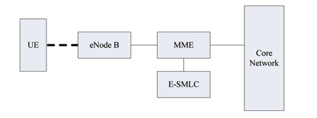
LTE location architecture is shown in Figure 1. The evolved serving mobile location center (E-SMLC) is the server component in charge of positioning activities. The mobility management entity (MME) gives the positioning request to E-SMLC, which then controls the user equipment (UE, the LTE device to be positioned) and, possibly, LTE base stations (eNodeBs), to perform positioning.
LTE Positioning Protocol. The actual positioning and assistance protocol between E-SMLC and UE is called LTE Positioning Protocol (LPP). In overview, LPP consists of three independent elementary procedures: capability exchange, assistance data exchange, and location information exchange, which refers to both measurement and position. The associated messaging is shown in Figure 2. In addition to the six message types shown, there are LPP Error and LPP Abort messages to handle abnormal situations.
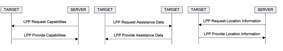
Figure 3 shows a sample positioning session using all the procedures. Assume that the server has received a location request for a given target (UE) and that the server can exchange messages with the UE — that is, lower protocol layers can provide the transport for the LPP-level messages. The first transaction of the location session is the capability exchange (LPP Request/Provide Capabilities). This information exchange makes the server aware of the UE positioning capabilities (GNSS support, supported cellular network measurements). Based on this information, the server can make a decision on the positioning method to be used, based on both UE capabilities and the requested quality-of-position (response time, accuracy).
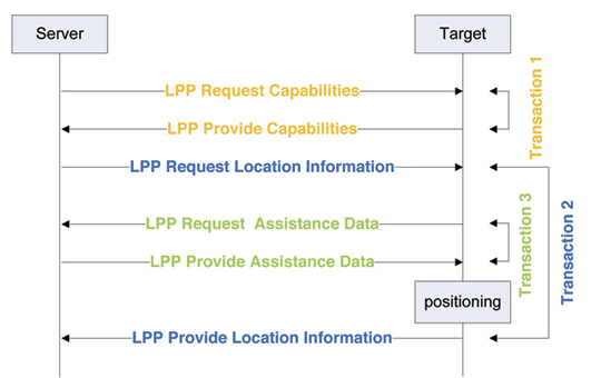
The actual location information request is carried in LPP Request Location Information message: whether position or measurements are requested and/or allowed and, for instance, which GNSSs are allowed to be used. It also carries other reporting instructions such as periodicity and required response time.
Having received this message, the target begins its positioning activities. In a typical scenario, this activity triggers a request for the assistance data. For instance, if the server requests the GNSS-based position, and the target does not have the latest ephemerides, the target will request those with the LPP Request/Provide Assistance Data mechanism (transaction 3). Having received the ephemerides, the target can position itself quickly, without needing the data broadcasts from the satellites, and report the location information back to the server in LPP Provide Location Information message. Other supporting information, such as reference location, reference time and ionosphere model, may also be provided to the target.
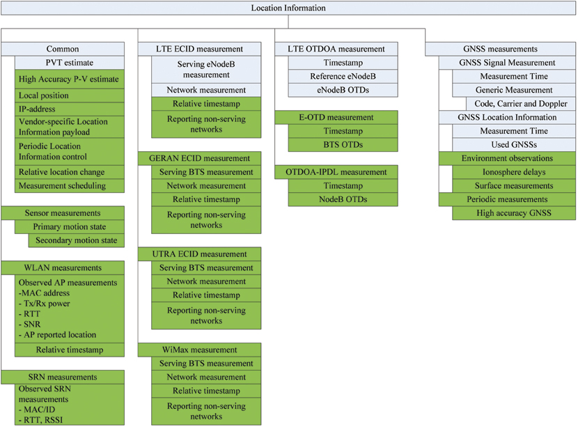
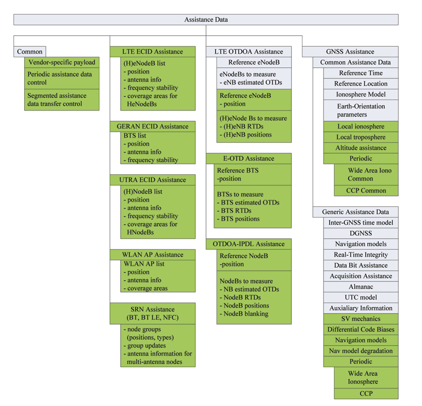
Figures 4 and 6 summarize the contents of LPP Provide Location Information and LPP Provide Assistance Data messages, respectively, in the gray boxes. The LPP Provide Location Information contents can be roughly divided into four categories: one category for each positioning method (assisted GNSS, observed TDOA, and ECID) and one category for providing the location estimate. In the A-GNSS category, the UE, based on the server commands, either reports the raw code and carrier-phase measurements (UE-assisted mode) or information regarding the provided PVT estimate (OTDOA and ECID function only in UE-assisted mode in LPP).
The LPP Provide Assistance Data reflects the same structure and categorization. Similarly, to Provide Location Information message, one can see in the assistance data message GNSS-specific assistance as well as OTDOA-specific assistance. However, there is no ECID-specific assistance due to it being available only in UE-assisted fashion. For OTDOA there is assistance, but only to assist the UE in the measurement process, not for positioning purposes — for instance, eNodeB positions cannot be transferred in the assistance data.
User Plane and Applications. RRLP, RRC, and LPP are natively control-plane positioning protocols. This means that they are transported in the inner workings of cellular networks and are practically invisible to end users. In the control pla
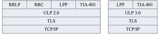
ne, their main purpose is to reliably provide the emergency-call positioning capability. However, there is obviously demand for positioning services for location-based end-user applications. To address this, in 2003 the Open Mobile Alliance started to work with Secure User Plane Location (SUPL) 1.0 protocol that brings the same location capabilities to user plane (application domain) over IP-networks as RRLP/RRC/LPP bring to control plane. One design principle of SUPL was not to re-invent the wheel; thus RRLP/RRC/LPP are being re-used in the user plane domain for positioning. OMA SUPL specifies a bearer protocol that carries a 3GPP-defined positioning protocol and provides security, authentication, privacy, and charging mechanisms. SUPL 1.0 is already commercially deployed, and SUPL 2.0 is now being deployed globally.
Figure 5 shows the OMA SUPL 2.0 protocol stack, which illustrates the re-use of 3GPP positioning protocols over IP networks. The security is provided by the standard transport layer security (TLS), and the user plane location protocol (ULP) is the wrapper for the 3GPP positioning protocols. The vast majority of SUPL 2.0 deployments will use RRLP as the positioning protocol. SUPL 3.0, currently being defined, will no longer support RRLP/RRC; LPP will gradually replace RRLP as the dominant standardized positioning protocol.
LPP Extensions
From the beginning, it was clear that the contents of the LPP would largely reflect that of the RRLP and would be limited to the native capabilities in the GNSS domain, and in other positioning methods to the methods strictly needed to fulfill the emergency-call positioning requirements. For example, in the GNSS domain the ionosphere models are limited to the (global) broadcast models as obtained from GPS, QZSS, and Galileo; there is no support for local ionosphere models. Other potential performance improvements including troposphere models and pressure-based altitude assistance are not in the scope of the 3GPP LPP work. Furthermore, a plethora of other positioning methods ranging from GSM- and WCDMA-based positioning (ECID, hyperbolic TDOA methods) to utilizing WLAN and short-range nodes such as Bluetooth are beyond the scope of current LPP development.
During the LPP Release 9 work, the industry was at a crossroads. On one hand, it was known that the 3GPP-defined LPP would become the de facto standardized protocol to do basic positioning not only in the LTE control plane, but also in IP networks over SUPL 2.0 and 3.0. On the other hand, it was also known that it would lack some key features including WLAN-based positioning, which would essentially force vendors to introduce proprietary protocols to augment LPP. Further, a serious drawback for use of LPP in the IP-network domain is that it does not support GSM- and UTRA-specific positioning methods (ECID, OTDOA). Thus, LPP could not completely replace legacy positioning protocols, including RRLP.
These considerations led to discussion of introducing extension hooks in LPP messages, so that the bodies external to 3GPP could extend the LPP feature set. In 2009, Qualcomm contributed extension containers to the LPP messages, and the way was open to start work on OMA LPP Extensions Release 1.0 in 2010.
The mandate of the OMA LPP Extensions (LPPe) is to build on top of the 3GPP LPP, re-using its procedures and data types as far as possible. This means that the message types are fixed; new messages cannot be defined, only extensions to existing ones can be formulated. Whenever possible, OMA should re-use information elements from 3GPP LPP to avoid duplicate definitions, compatibility, and maintenance issues. LPPe is supported in SUPL 3.0, which will be the primary transport protocol of LPPe.
Procedure Extensions. OMA LPP Extensions Release 1.0 not only defines new positioning methods and assistance data types, but also defines new procedures for improved performance. These include the following:
◾ Capability exchange and location-information exchange reversed mode, illustrated in Figure 7, with the LPPe Request/Provide Capabilities/Location Information messages flowing in the opposite directions as compared to Figure 2. This reversed mode is only allowed in the context of LPPe. In the context of assistance data support, capabilities in the reversed case refer to the assistance data that the server can provide, as opposed to the assistance data the target can utilize in normal mode-capability exchange.
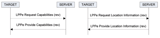
The interpretation of reversed mode for location information exchange is somewhat more delicate. When the UE sends LPPe Request Location Information to the server, the UE does not request the server position, but the UE position. In the request the UE may define the quality-of-position, which then guides the positioning method selection by the server.
- Periodic assistance data is a completely new feature to the assistance-data protocols. Periodic assistance can be used with selected assistance-data types that require updates at short intervals. Such data types include short-term real-time ionosphere correction from GNSS networks and carrier phase — assistance for high-accuracy relative positioning. The periodic assistance procedure also includes the possibility for the target and server to update the periodic session-control parameters (duration, rate of delivery) intra-session. This control is carried in the common part of the LPPe Request/Provide Assistance Data message (Figure 6).
- Periodic location information reporting is included in 3GPP LPP, but the similar capability in the OMA LPPe is specifically designed for continuous measurements including continuous carrier-phase measurements for high-accuracy purposes. The 3GPP LPP does specify periodic measurements, but in such a way that, say, the GNSS measurement engine can be powered off between measurement deliveries, which is obviously unacceptable in the view of carrier-phase-based relative high-accuracy GNSS. The periodic location information procedure also includes the possibility for the target and server to update the periodic session-control parameters (duration, rate of delivery) intra-session. This control is carried in the common part of the LPPe Request/Provide Location Information message as shown in Figure 4.
- Segmented assistance-data transfer procedure allows for partitioning a large assistance-data delivery into smaller segments as well as resuming such a segmented session after an active-inactive-active cycle in the LPPe session. This control is carried in the common part of the LPPe Request/Provide Assistance Data message as shown in Figure 6.
- Measurement scheduling/windowing allows the server to request measurements (GNSS, ECID, TDOA) to be made within a certain time window that can be expressed in terms of GNSS time or cellular network time. This control is carried in the common part of the LPPe Request/Provide Location Information message as shown in Figure 4.
Extensions. OMA LPPe introduces several enhancements for various positioning methods as well as completely new methods:
- Additions in the A-GNSS domain include local atmosphere models. In 3GPP LPP, the models are limited to ionosphere ones and therein to the broadcast types as in GPS, Galileo, and QZSS broadcasts. The OMA LPPe introduces a localized Klobuchar model, which allows for presenting the delay corrections in the well-known Klobuchar model, but for a limited-validity area and time for more accurate delay compensation. In addition, ionosphere storm warnings can be carried to the UE at the chosen resolution. This information allows UE to deduce the reason for high measurement residuals.
Troposphere models have not previously been in the scope of the standardized assistance protocols. The troposphere model in LPPe carries the hydrostatic and wet zenith delays, their change rates in the height dimension for approximating the zenith delays at the UE altitude, Niel mapping functions for hydrostatic and wet components, and composite spatial gradients. Alternatively, the surface meteorological parameters (pressure, temperature) can be carried to the UE, and the calculation of the troposphere delay is left for the UE.
Another troposphere model is the altitude-pressure relationship for the UEs with a barometer. This altitude assistance increases availability by introducing an independent source of altitude information.
Whereas the 3GPP LPP carries the ephemerides, almanacs, signals supported by the satellites, and the GLONASS frequency mappings, OMA LPPe introduces satellite mechanical informational, differential code biases, and new navigation models. The mechanical information consists of mass, effective reflectivity-area, and phase-center offsets for the in-UE orbit prediction purposes. In the navigation model domain, the additions include SP3-type orbit representation and the orbit/clock model degradation models for improved error modeling. Practically all the new assistance data types support precise-point positioning approaches for future GNSS services.
Lastly, one of the major LPPe A-GNSS features is the continuous carrier-phase (CCP) assistance for real-time kinematic applications. The CCP data format supports straightforward mapping from RTCM 10403.1 to ensure interoperability. The LPPe CCP mechanism utilizes the LPPe-level periodic assistance data procedure and supports multiple reference stations as well as mobility, that is, changes in the set of active reference stations on-the-fly.
- To enable the use of LPP/LPPe in all the networks, the legacy hyperbolic methods E-OTD and OTDOA-IPDL for GSM and UTRA networks, respectively, are supported, and the data content are copy/pastes from RRLP and RRC to ensure interoperability. Support for UE-based LTE OTDOA is also included.
- A major part of LPPe specification is devoted to the various ECID methods. These cover GSM, UTRA, LTE, and WLAN networks both in UE-assisted and UE-based modes.
- In LPPe terminology, the short-range nodes (SRNs) refer to Bluetooth, Bluetooth Low-Energy, and near-field communication (NFC) tags, which are considered separately from the primary communications networks (cellular networks and WLAN). Similarly to the ECID methods, the SRNs can be used for positioning in either UE-assisted or UE-based modes. In the UE-based mode, in which the SRN locations need to be carried to the UE, the philosophy is that the SRNs are logically arranged into groups – one group of SRNs can be the set of SRNs in one building or in one floor in the building. The assistance data is considered in the units of these groups in conjunction with the group data version that allows for handling situations, in which the arrangement of the SRNs in the building changes, and the data in the UE needs to be refreshed.
- Finally, no single positioning and assistance protocol can address all needs. Thus, both LPPe assistance data exchange and LPPe location information exchange include black-box containers for vendors and operators to carry their own proprietary assistance data and location information in a standardized framework. The benefit of this approach is that the same standardized protocol framework used in commercial deployments can be used for rapid prototyping and providing differentiating positioning performance, without the need for defining proprietary protocols from scratch.
Conclusion
The framework introduced by 3GPP LPP and extended in LPPe brings long-sought convergence in the control- and user-plane positioning protocols. This ensures that in the user-plane domain, the dominant domain for positioning services in consumer LBS, vendors can utilize exactly the same protocol as in the control plane. This reduces implementation, testing, and deployments costs, and will make the LPP/LPPe the de facto standardized positioning protocol in the mobile domain.
Lauri Wirola has a Ph.D. in electrophysics from Tampere University of Technology in Finland. He manages indoor positioning activities at Nokia Services Location.


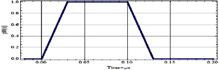
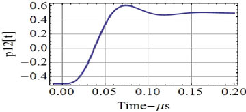
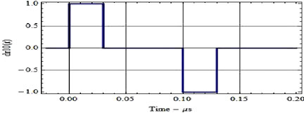 FIGURE 2. Trapezoidal PN (1 Mcps) waveform pulse and its time derivative with a 0.1-microsecond rise time.
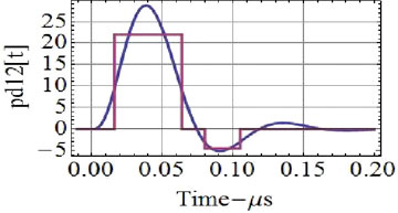
![FIGURE 3. Discriminator channel, d[e], and (bottom) discriminator output, R[e] Rd[e], for the 1.0 Mcps PN with the optimum 0.1-microsecond reference and the 0.1-microsecond rise-time trapezoidal waveform.](https://stage.globalpositioningnews.com/wp-content/uploads/2010/05/EA-3.jpg)