The U.S. Department of Transportation will host a third workshop to continue discussions of the GPS Adjacent Band Compatibility Assessment on March 12.
The workshop will focus on the following topics:
Identification of GPS and GNSS receivers to be considered for testing that are representative of the current categories of user applications
Discussion of a GPS/GNSS receiver test plan.
Anyone interested in presenting on either or both of the above topics should contact Stephen Mackey by March 2.
The workshop will be held 8:30 a.m.-3:30 p.m. PDT at Aerospace Corporation, 2310 E. El Segundo Blvd., El Segundo, California.
Orteco is an Italian manufacturer of pile-driving equipment.
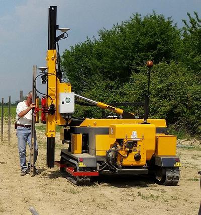
Orteco, a specialized manufacturer of pile driving machines based in northern Italy, has introduced a series of robotic pile drivers using APS-U GNSS RTK receivers from Altus Positioning Systems. The products are being supplied to Orteco by Altus’ parent company, Septentrio NV.
The driverless tracked crawler maneuvers automatically under control of the APS-U, which provides centimeter-level position coordinates and heading information within 0.3 degrees, following a project map loaded into the machine’s computer. It automatically drives itself to each location, positions the mast and drives the post in a perfectly vertical position, stopping the installation at exactly the desired height, then moves automatically to the next spot.
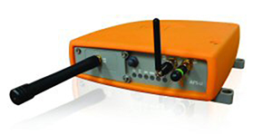
The Altus APS-U-HDG is a high-precision 272-channel GPS/GLONASS/SBAS receiver with dual antennas designed to provide highly accurate heading and position for machine control applications. Cased in a rugged MIL-STD-810C aluminum housing, the instrument is built to the most rigorous standards for waterproofing, humidity, dust, shock, vibration and extreme temperatures.
The Altus APS-U-HDG.
Orteco is building the GNSS-controlled pile driver in various configurations for applications such as photovoltaic farms, fences, roadside barriers and agriculture. It makes pile driving jobs faster, safer and more accurate with fewer workers, increasing productivity and reducing costs, Altus said.
“The Orteco machines provide a perfect demonstration of the ruggedness, power and performance of the APS-U as a highly accurate heading and positioning sensor in one of the most demanding environments imaginable,” said Altus CEO Neil Vancans. “In extensive tests conducted by Orteco, the APS-U receivers proved themselves up to the task, performing reliably under the constant heavy pounding and vibration of the pile driver.”
Based in Bologna, Orteco is a specialized manufacturer focused on pile driving with a 40-year history. In 2011, the company reached a milestone of 1,000 pile drivers produced and distributed all over the world. The company’s GNSS-controlled agricultural pile driver, designed to install posts in large vineyards, was recognized as a winner of the Innovation Challenge Enovitis in campo 2014 by Unione Italiana Vini and Veronafiere.
Centimeter Positioning with a Smartphone-Quality GNSS Antenna
By Kenneth M. Pesyna, Jr., Robert W. Heath, Jr. and Todd E. Humphreys, the University of Texas at Austin
The smartphone antenna’s poor multipath suppression and irregular gain pattern result in large time-correlated phase errors that significantly increase the time to integer ambiguity resolution as compared to even a low-quality stand-alone patch antenna. The time to integer resolution — and to a centimeter-accurate fix — is significantly reduced when more GNSS signals are tracked or when the smartphone experiences gentle wavelength-scale random motion.
GNSS chipsets are now ubiquitous in smartphones and tablets. Yet the underlying positioning accuracy of these consumer-grade GNSS receivers has stagnated over the past decade. The latest clock, orbit, and atmospheric models have improved ranging accuracy to a meter or so, leaving receiver-dependent multipath and front-end-noise-induced variations as the dominant sources of error in current consumer devices. Under good multipath conditions, 2-to-3-meter-accurate positioning is typical; under adverse multipath, accuracy degrades to 10 meters or worse.
Yet outside the mainstream of consumer GNSS receivers, centimeter — even millimeter — accurate GNSS receivers can be found. These high-precision receivers are used routinely in geodesy, agriculture, and surveying. Their exquisite accuracy results from replacing standard code-phase positioning techniques with carrier phase differential GNSS (CDGNSS) techniques. Currently, the primary impediment to performing CDGNSS positioning on smartphones lies not in the commodity GNSS chipset, which actually outperforms survey-grade chipsets in some respects, but in the antenna, whose chief failing is its poor multipath suppression. Multipath, caused by direct signals reflecting off the ground and nearby objects, induces centimeter-level phase measurement errors, which, for static receivers, have decorrelation times of hundreds of seconds. The large size and strong time correlation of these errors significantly increases the initialization period — the so-called time-to-ambiguity-resolution (TAR) — of GNSS receivers employing CDGNSS to obtain centimeter-level positioning accuracy.
Prior work on centimeter-accurate positioning with low-cost mobile devices has focused on external devices, or “pucks,” which contain a GNSS antenna and chipset. These devices interface with the smartphone via Bluetooth or a wired connection. Such solutions, which enjoy the better sensitivity and multipath suppression offered by their comparatively large, high-quality GNSS antennas, do not provide insight into the feasibility of CDGNSS on a stand-alone smartphone platform.
This article demonstrates that centimeter-accurate CDGNSS positioning is indeed possible based on data sampled from a smartphone-quality GNSS antenna. This result has far-reaching significance for precise mass-market positioning. We offer an empirical analysis of the average gain and carrier phase multipath error susceptibility of smartphone-grade GNSS antennas. We also demonstrate that, for low-quality GNSS antennas such as those in smartphones, wavelength-scale random antenna motion substantially improves the time to integer ambiguity resolution.
This article focuses on single-frequency CDGNSS rather than multiple-frequency CDGNSS or other carrier-phase-based techniques, such as precise-point positioning (PPP), for three reasons. First, virtually all smartphones are equipped with single-frequency GNSS antennas tuned to the L1 band centered at 1575.42 MHz, and single-frequency CDGNSS will likely forever remain the cheapest option. Second, as compared to PPP, CDGNSS converges much faster to centimeter accuracy, which will be important for impatient smartphone users.
Finally, as centimeter-accurate GNSS moves into the mass market, GNSS reference stations will proliferate so that the vast majority of users can expect to be within a few kilometers of one. In this so-called short baseline regime, the differential ionospheric delay between the reference and mobile receivers becomes insignificant, obviating differential delay estimation via multi-frequency measurements. Of course, the additional signal measurements produced by multiple-frequency receivers would lead to faster convergence times and improved robustness, but for many applications, single-frequency measurements will be adequate.
Test Architecture
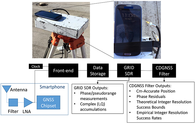
We used the test architecture shown in Figure 1 to collect data from a smartphone-grade antenna and higher quality antennas, process these data through a software-defined GNSS receiver, and compute a CDGNSS solution on the basis of the carrier phase measurements output by the GNSS receiver.
Figure 1. Test architecture designed for an in-situ study of a smartphone-grade GNSS antenna. The analog GNSS signal is tapped off after the phone’s internal bandpass filter and low-noise amplifier and is directed to a dedicated RF front-end for downconversion and digitization. Data are stored to file for subsequent post-processing by a software GNSS receiver and CDGNSS filter.
The architecture has been designed such that the antenna is left undisturbed within the phone; data are collected by tapping off the analog signal immediately after the phone’s internal bandpass filter and low-noise amplifier. This analog signal is directed to an external radio frequency (RF) front-end and GNSS receiver. Use of an external receiver permits well-defined GNSS signal processing unencumbered by the limitations of the phone’s internal chipset and clock.
The clock attached to the external front-end was an oven-controlled crystal oscillator (OCXO), which has much greater stability than the low-cost oscillators used to drive GNSS signal sampling within smartphones. However, it was found that reliable cycle-slip-free GNSS carrier tracking only required a 40-ms coherent integration (pre-detection) interval, which is within the coherence time of a low-cost temperature-compensated crystal oscillator (TCXO) at the GPS L1 frequency.
Although only a single model of smartphone was tested using this architecture — a popular mass-market phone — the results are assumed representative of all smartphones from the same manufacturer.
Using this architecture, many hours of raw high-rate (∼6 MHz) digitized intermediate frequency samples were collected and stored to disk for post processing. Also stored to disk were high-rate data from a survey-grade antenna, which served as the reference antenna for CDGNSS processing. An in-house software-defined GNSS receiver, known as GRID, was used to generate, from these samples, high-quality carrier phase measurements. GRID is a flexible receiver that can be easily adapted to maintain carrier lock despite severe fading. Complex baseband accumulations output from GRID allowed detailed analysis of the signal and tracking loop behavior to ensure that no cycle slips occurred. The generated carrier phase measurements were subsequently passed to a CDGNSS filter, a model for which is described in the next section.
CDGNSS Processing
The CDGNSS filter described in this section ingests double-differenced carrier phase measurements output from GRID and processes them to produce (1) the centimeter-accurate trajectory estimate of the mobile antenna, (2) a time history of phase residuals, (3) carrier phase integer ambiguity estimates, (4) theoretical integer ambiguity resolution success bounds, and (5) empirical integer ambiguity resolution success rates. These outputs are used to analyze the performance of the smartphone-grade antenna and compare its performance to higher-quality antennas.
CDGNSS Filter Model. The filter’s state has a real-valued component xk that models the mobile antenna’s relative center of motion, its instantaneous offset from this center of motion, and its velocity at each time epoch k:
. (1)
The filter’s state also has an integer-valued component that models the CDGNSS phase ambiguities:
(2)
where NSV is the total number of satellites tracked. Such integer ambiguities are inherent to carrier phase differential positioning techniques; their resolution has been the topic of much past research and is required to produce a CDGNSS positioning solution.
Dynamics and Measurement Models. The real-valued state component xk is assumed to evolve as a mean-reverting second-order Gauss-Markov process. This process models the time-correlated and mean-reverting motion a smartphone experiences when held or moved gently in the extended hand of an otherwise stationary user. The integer-valued state component nk is modeled as constant, since the phase ambiguities remain fixed so long as the receiver retains phase lock on each signal.
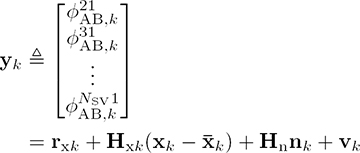
The filter ingests measurement vectors yk for k = 1, …, K, each populated with a single epoch of double-differenced carrier phase measurements for i = 1, 2, . . . , NSV–1. The filter’s measurement model relates yk to the real- and integer-valued state components through the following linearized GNSS carrier phase measurement model:
(3)
where rxk is a vector of double-differenced modeled ranges based on the filter’s real-valued state prior ,Hxk and Hn are the measurement sensitivity matrices for the real- and integer-valued state components, and vk is the double-differenced measurement noise vector, all at time k.
Phase Residuals. After processing data through the CDGNSS filter, the filter outputs, in addition to a time history of centimeter-accurate position estimates, a time history of phase residuals , which can be thought of as departures of each double-differenced phase measurement from phase alignment at the phase center of the antenna. These residuals can be modeled as
(4)
where rxk is now based on the filter’s real-valued state estimate at time k and represents the filter’s estimate of the integer ambiguities at time K.
Phase residuals have been produced for batches of data collected from four different grades of antennas, as described next. These residuals will be used to analyze the suitability of each antenna for CDGNSS positioning.
Antenna Performance Analysis
This section describes four antennas from which data were captured and processed using the test architecture and CDGNSS filter described previously. It also quantifies the characteristics that make low-quality smartphone-grade antennas poorly suited to CDGNSS.
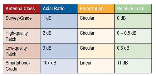
Table 1 describes a range of antenna grades of decreasing quality, noting properties relevant to CDGNSS. The loss numbers in the far-right column represent the average loss in gain relative to a survey-grade antenna, where the average is taken over elevation angles above 15 degrees.
Table 1. Antenna properties.
Survey-grade antennas, whose properties are described in the first row of Table 1, have a uniform quasi-hemispherical gain pattern, right-hand circular polarization, a stable phase center, and a low axial ratio. These are all desirable properties for CDGNSS. Unfortunately, these properties inhere in the antennas’ large size; the laws of physics dictate that smaller antennas will typically be worse in each property.
The last row of Table 1 lists the properties for a smartphone-grade antenna. As shown subsequently, this antenna loses between 5 and 15 dB in sensitivity as compared to the survey-grade antenna. Such a loss makes it difficult to retain lock on GNSS signals. In addition, this antenna’s linear polarization leads to extremely poor multipath suppression.
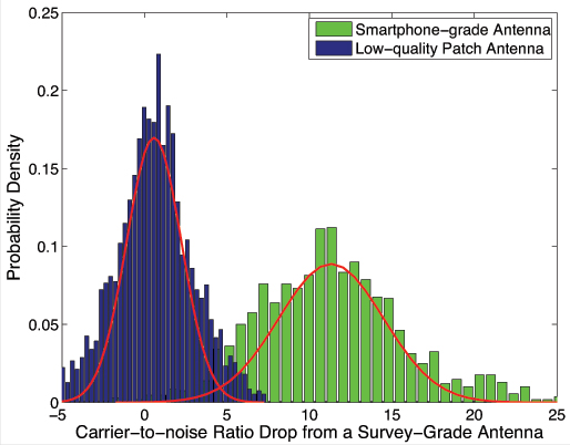
Antenna Gain Analysis.Figure 2 quantifies one of the obvious drawbacks of a smartphone-grade antenna, namely, its low gain.
Figure 2, Drop in carrier-to noise ratio, from 2 hours of data and 9 tracked satellites. Antennas remained stationary.
The rightmost histogram, in green, shows that the decrease in carrier to noise ratio as compared to a survey-grade antenna is on average 11 dB, such that the smartphone-grade antenna only captures approximately 8 percent of the signal power as compared its survey-grade counterpart. For comparison, shown on the left, in blue, is a histogram of the decrease in carrier-to-noise ratio for the low-quality patch antenna. This antenna only suffers about a 0.6-dB drop in power on average relative to the survey-grade antenna. Each histogram was generated from 2 hours of data with nine tracked satellites ranging in elevation from 15 to 90 degrees. The antennas remained stationary. The variation in signal power around the means is due to the multipath-induced power variations in the signal as well as to the different gain patterns between each antenna and the survey-grade antenna.
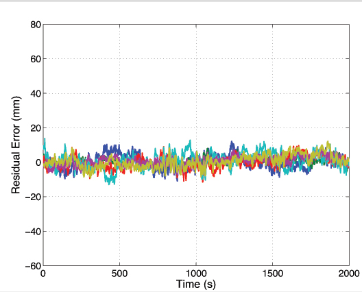
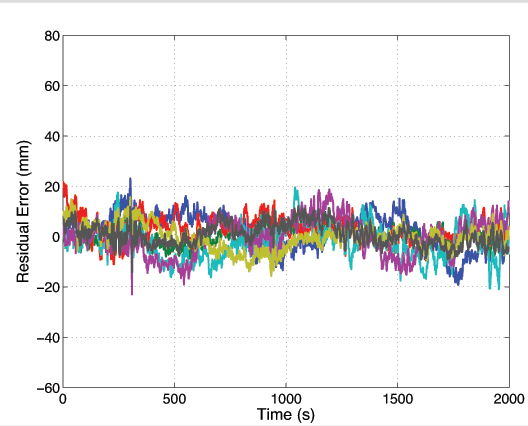
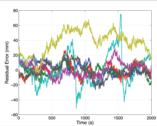
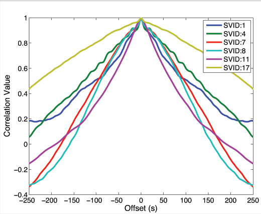
Phase Residual Analysis. Shown in Figures 3, 4, and 5 are 2,000-second segments of double-differenced phase residual time histories for data collected from a survey-grade, a low-quality patch, and a smartphone-grade antenna, respectively.
Figure 3. Survey-grade antenna. Each trace represents a residual for a different satellite pair. Ensemble average standard deviation 3.4 millimeters.Figure 4. Low-quality patch antenna. Ensemble average deviation 5.5 mm.Figure 5. Smartphone-grade antenna.Ensemble average deviation 11.4 mm.
To produce these residuals, the antenna position was locked to its estimated value within the CDGNSS filter. The residuals represent departures of the carrier phase measurements from perfect alignment at the average phase center of the antenna. Each different colored trace corresponds to a different satellite pair. While the data segments were not captured at the same time of day, they were captured at the same location, and thus the multipath environment was similar.
The ensemble average residual standard deviations increase with decreasing antenna quality. The residuals for the survey-grade, low-quality patch, and smartphone-grade antennas have ensemble average standard deviations of 3.4, 5.5 and 11.4 millimeters, respectively. This increase is due to the lower gain and less effective multipath suppression of the lower quality antennas.
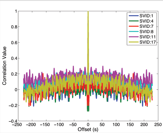
Figure 5 shows the presence of outlier residuals in the data collected from the smartphone-grade antenna. These outliers, one of which persists for over 1,000 seconds, are likely caused by either large and irregular azimuth- and elevation-dependent antenna phase center variations or a combination of poor antenna gain in the direction of the non-reference satellite coupled with ample gain in the direction of a multipath signal such that the multipath signal is received with more power than the direct-path signal. Obvious outliers such as these can be automatically excluded by the CDGNSS filter via an innovations test. However, the standard deviation of the remaining residuals still remains large compared to that of the other antennas; the ensemble average standard deviation decreases from 11.4 to 8.6 millimeters upon exclusion of the two large outliers.
For antennas with a large ensemble average standard deviation in their double-differenced phase errors, the time correlation in the phase errors becomes more important. This time correlation, which persists for 100–200 seconds, is a well-studied phenomenon caused by slowly varying carrier phase multipath. While correlation is present in the residuals of all antenna types, and manifests approximately the same decorrelation time, its effect is more of a problem for low-quality antennas because the phase errors are larger. Such correlation, coupled with a large deviation, ultimately leads to a longer time to ambiguity resolution, shown later.
Given a smartphone antenna’s extremely poor gain and multipath suppression as compared to even a low-quality stand-alone patch antenna, one might question the wisdom of attempting a CDGNSS solution using such an antenna. However, the next section reveals that it is indeed possible to achieve a centimeter-accurate positioning solution using a smartphone GNSS antenna despite its poor properties.
CDGNSS with Smartphone Antenna
Figure 6 shows the result of an attempt to compute a CDGNSS solution using data collected from the GNSS antenna of a smartphone. The cluster of red near the top of the phone represents 400 CDGNSS position estimates over a 5-minute interval, superimposed on the photo and properly scaled. This cluster is referenced to a marker immediately under the phone whose position was surveyed to approximately 1-centimeter accuracy using a high-quality patch antenna. The mean of the cluster’s horizontal coordinates is approximately 2 centimeters from the phone’s internal GNSS antenna. Figure 6 shows the absolute horizontal accuracy of a CDGNSS solution through the smartphone’s antenna is approximately 2 centimeters.
Figure 6 . Successful CDGNSS solution using data collected from smartphone antenna. The red cluster represents 400 CDGNSS solutions over 5 minutes, superimposed and properly scaled.
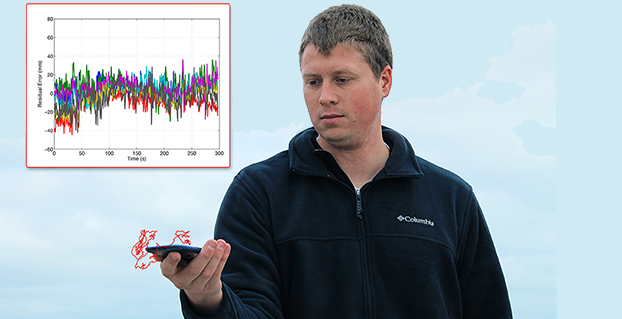
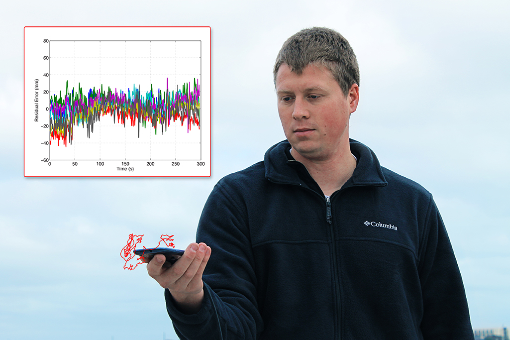
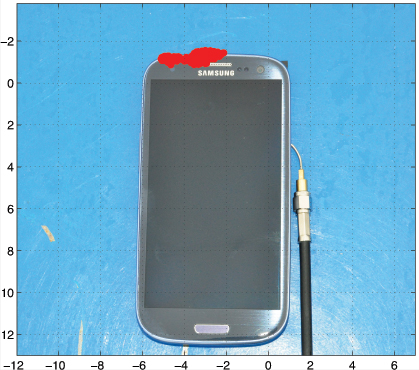
The data in Figure 6were collected with a large conductive backplane below the smartphone. However, the backplane is unnecessary. The opening photo shows the result of a CDGNSS positioning solution computed using data collected from the smartphone antenna while the device was held in the extended hand of the author. The cluster of red represents the computed 3-dimensional position of the phone over a 300-second interval, superimposed on the photo and properly scaled. The author’s hand moved slightly during the interval, as reflected in the figure.
The opening photo also shows the residuals corresponding to the handheld CDGNSS solution. This shows how the residuals look in practice for a scenario in which the phone is held by a user. The residuals look fairly clean, that is, they have a small variance and their mean is approximately zero. It is not uncommon for the residuals to look this good; however, cases do arise in which the residuals are considerably worse due to a combination of poor antenna gain in the direction of the non-reference satellite, coupled with ample gain in the direction of a multipath signal.
The possibility of CDGNSS-enabled centimeter positioning using a smartphone antenna has been previously conjectured, but — to our knowledge — Figure 6 and the opening photo represent the first published demonstrations that this is indeed possible. This significant result portends a vast expansion of centimeter-accurate positioning into the mass market. However, serious challenges must be overcome before mass-market CDGNSS can become practical. Some of these challenges will be studied in the next few sections.
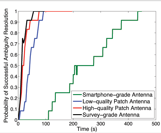
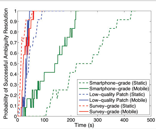
Static Scenario. Figure 7 shows the empirical probability of successful ambiguity resolution for data collected from four antennas, one of each of the different grades discussed earlier. For each antenna, seven satellites were tracked at approximately the same location and time of day. Each trace was computed from 12 batches of double-differenced carrier phase data.
Each trace represents an empirically-derived success rate computed from 12 batches of phase data as follows:
For a given batch, at each epoch the filter outputs its best estimate of the integer ambiguities on the basis of the data ingested thus far.
The estimate from step 1 is compared against the true set of integer ambiguities which were acquired in advance by processing a much longer batch of data. If correct, a flag is set at that epoch to “1”; if incorrect, the flag is set to 0.
For each epoch, the flags produced in step 2 are averaged across all 12 batches to generate each trace.
Figure 7. Residuals for CDGNSS solution depicted in the opening photo.
As shown by the green trace in Figure 7, the smartphone-grade antenna required 400 seconds to achieve a 90% ambiguity resolution success rate; in other words, it manifested a 400-second TAR at 90%. This would surely exceed the patience of most smartphone users. Also shown are traces for the other three antenna grades. The higher-quality antennas yield shorter TARs for a given success rate, primarily due to their superior multipath suppression.
Note that the loss in received signal power due to the smartphone antenna’s poor gain turns out to be tolerable — the signals arriving from the smartphone-grade antenna can be tracked without cycle slipping. Therefore, the outstanding challenge preventing fast ambiguity resolution for data collected from smartphone-grade antennas is the severe time-correlated multipath errors in the double-differenced carrier phase data.
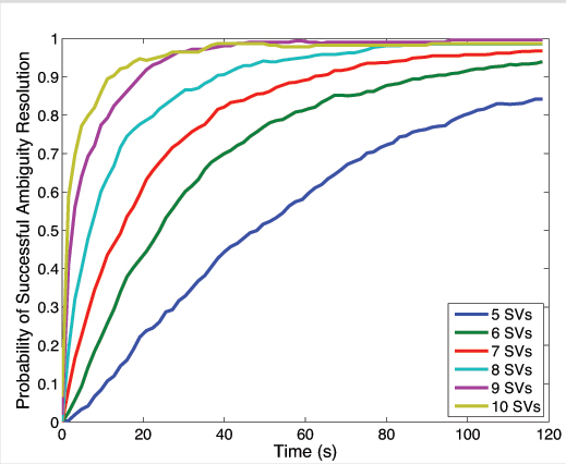
Decreasing TAR via More Signals. There are ways to mitigate the impact of multipath on the CDGNSS TAR, even the severe multipath experienced by low-quality antennas. It has been shown that the volume of the integer ambiguity search space, and thus TAR, decreases as a function of the number of double-differenced phase time histories available, which, for single-frequency CDGNSS, is one less than the number of satellites tracked. Consequently, an acceptable TAR can always be achieved with enough satellites tracked.
Figure 8 shows the reduction in TAR for an increasing number of satellites. Each trace was computed from 720 non-overlapping 2-minute batches of data taken from a survey-grade antenna over a 24-hour interval. A decreasing elevation mask angle was used to allow an increasing number of SVs to participate in the CDGNSS solution. For a given 2-minute batch of data, an elevation mask was first applied to all but the highest five satellites. Double-difference phase data from these satellites were then processed by the CDGNSS filter to compute an empirical probability of successful integer ambiguity resolution. Next, the elevation mask was reduced until one additional satellite was in view, and the process repeated to produce all traces shown.
Figure 8 makes clear that each additional double-differenced phase time history, although corrupted by its own multipath-induced phase errors, significantly decreases the overall TAR. Note that although Figure 8 was produced from data collected via a survey-grade antenna, a similar trend would apply for the smartphone-grade antenna. One implication of Figure 8 is that smartphone-based CDGNSS would benefit greatly from the additional double-differenced measurements that a multi-frequency GNSS receiver could provide. For example, at the time of writing there are 14 operational GPS satellites broadcasting unencrypted civil signals at the GPS L2 frequency (1227.6 MHz), and 7 broadcasting civil signals at the GPS L5 frequency (1176.45 MHz). With some modification of the smartphone GNSS antenna and chipset, these modernized GPS signals could be exploited to reduce TAR. However, the narrow profit margins on mass-market GNSS antennas and chipsets militate against multi-frequency architectures.
Figure 8. Probability of successful ambiguity resolution vs. time as a function of the number of satellite vehicles (SVs) tracked.
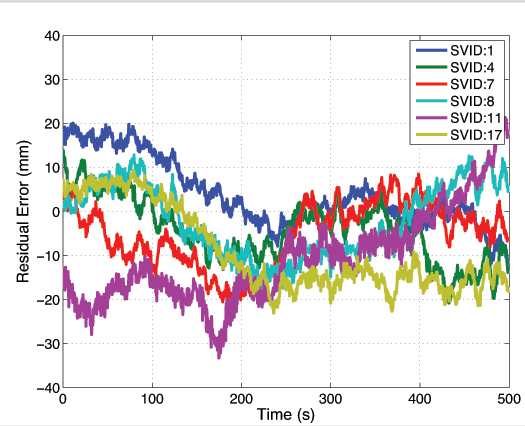
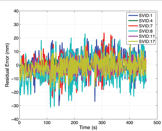
Decreasing TAR via Random Motion. There is a second way to reduce TAR under severe multipath conditions. Unlike TAR reduction via additional signals, the theory and practice of this second technique have not been previously treated in the literature. Moreover, the technique is well-suited for smartphones, which are typically hand-held and mobile. This simple technique consists of gently moving the smartphone in a quasi-random manner within a wavelength-scale volume. The key to this technique’s effectiveness is that, whereas multipath-induced phase measurement errors are typically time-correlated on the order of hundreds of seconds for a static receiving antenna, their spatial correlation is on the order of one wavelength, or approximately 19 centimeters at the GPS L1 frequency. As a result, random wavelength-scale antenna motion transforms the phase residuals from slowly-varying when the antenna is static, as shown in Figure 9, to quickly-varying when the antenna is dynamic, as shown in Figure 10.
Figure 9. Residuals for data captured from smartphone-grade antenna while static.Figure 10. Data from smartphone-grade antenna as it experienced wavelength-scale random motion, 2–5 cm/second.
Put another way, autocorrelation time of the phase residuals decreases from hundreds of seconds when the antenna is static, as shown in Figure 11, to less than a second when the antenna is moved even slowly (a few centimeters per second), as shown in Figure 12. More vigorous antenna motion would be possible if the phone’s inertial devices were used to aid the phase tracking loops.
Figure 11. Autocorrelation functions corresponding to the phase residuals in Figure 9.Figure 12. Autocorrelation functions corresponding to phase residuals in Figure 10.
The shorter phase error decorrelation time resulting from random antenna motion effectively increases the information content per unit time that each double-differenced phase measurement provides to the CDGNSS filter, thus decreasing the time to ambiguity resolution.
Figure 13 compares empirical success rates for three different antennas under static and dynamic scenarios. As expected, motion reduces the time-to-ambiguity resolution for the smartphone-grade and low-quality patch antenna. But, somewhat counterintuitively, motion increases the TAR for the survey-grade antenna. This discrepancy reflects a tradeoff within the CDGNSS filter. While it is true that the phase measurement errors decorrelate much faster when the antenna is moving — increasing the per-epoch information provided to the filter — it is also the case that the filter can no longer employ a hard motion constraint. For the high-quality antennas, the increased information per epoch due to faster phase error decorrelation is completely counteracted by a loss in information per epoch due to uncertainty (lack of constraint) in the motion model. Also, for the high-quality antennas, multipath in the reference antenna’s phase measurements is not insignificant compared to multipath in the mobile antenna, and this reference multipath exhibits the usual 100–200 second correlation time for a static antenna. On the other hand, phase error decorrelation via random antenna motion offers the lower-quality antennas a larger net information gain because their multipath-induced phase errors are so large. Consequently, for the smartphone-grade antenna, motion substantially reduces the 90 percent success TAR, which drops from 400 to 215 seconds.
Figure 13. Probability of successful ambiguity resolution versus time for three different antennas under static and dynamic scenarios.
Conclusions and Future Work
Centimeter-accurate positioning was demonstrated based on data sampled from a smartphone-quality GNSS antenna. An empirical analysis revealed that the extremely poor multipath suppression of these antennas is the primary impediment to fast resolution of the integer ambiguities that arise in the carrier phase differential processing used to obtain centimeter accuracy. It was shown that, for low-quality smartphone-grade GNSS antennas, wavelength-scale random antenna motion substantially reduces the ambiguity resolution time.
Future work will study the effectiveness of combining antenna motion with a motion trajectory estimate derived from non-GNSS smartphone sensors to further reduce the integer ambiguity resolution time. This technique, which is a type of synthetic aperture processing applied to the double-differenced GNSS phase measurements, effectively points antenna gain enhancements in the direction of the overhead GNSS satellites, thereby suppressing multipath arriving from other directions. Preliminary results show that this technique offers modest benefit beyond the unaided random motion technique discussed herein.
Acknowledgment
The material in this article was first presented at ION GNSS+ 2014 in the paper “Centimeter Positioning with a Smartphone-Quality GNSS Antenna.”
Kenneth M. Pesyna, Jr. is a Ph.D. candidate in the Department of Electrical and Computer Engineering at the University of Texas at Austin. He is a member of the University of Texas Radionavigation Laboratory and the Wireless Networking and Communications Group.
Robert W. Heath, Jr. is a Cullen Trust Endowed Professor in Electrical and Computer Engineering at UT-Austin, and director of the Wireless Networking and Communications Group. He received his Ph.D. in electrical engineeringfrom Stanford.
Todd E. Humphreys is an assistant professor in the department of Aerospace Engineeringand Engineering Mechanics at UT-Austin, and director of the UT Radionavigation Laboratory. He received a Ph.D. in aerospace engineering from Cornell University.
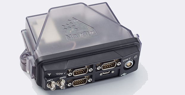
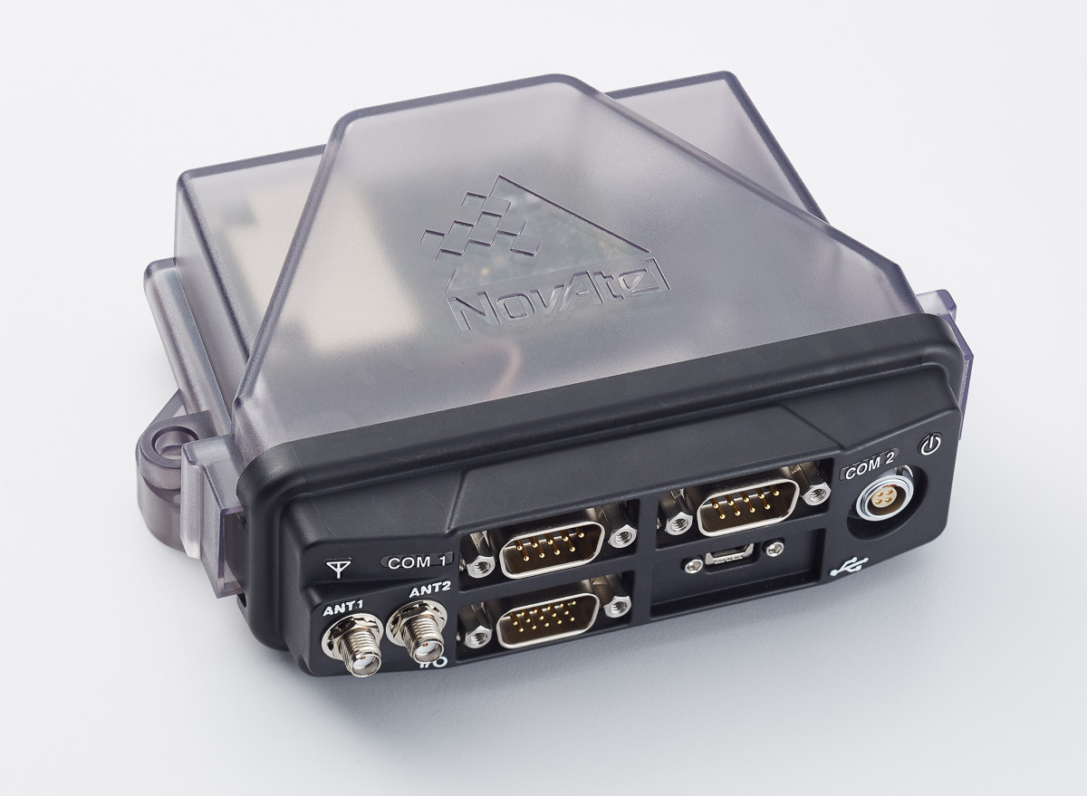
NovAtel Inc. has announced the FlexPak6D enclosed GNSS receiver, a flexible dual-antenna solution for application developers seeking a high-precision heading-capable positioning engine for space-constrained applications.
Designed for efficient and rapid integration, the compact, lightweight receiver tracks GPS, GLONASS, Galileo and BeiDou. Antenna placement is flexible, which means the antenna baseline can be set according to space available on the vehicle and the heading accuracy required. In addition, the modular nature of the FlexPak6D’s OEM6 firmware provides users with the ability to configure the receiver for their unique application needs.
Scalable for sub-meter to centimeter-level positioning, the FlexPak6D delivers NovAtel’s ALIGN precision heading and relative heading firmware, as well as its GLIDE firmware for smooth decimeter-level pass-to-pass accuracy, and RAIM for increased GNSS pseudorange integrity.
“Our FlexPak6D builds on our popular lightweight FlexPak form factor,” said Jason Hamilton, vice president of marketing for NovAtel. “The modular, flexible design makes it easy to integrate into land, air and marine-based industries, particularly for low payload UAV and robotic applications.”
The FlexPak6D will be available for shipping February 2, 2015.
A new module produced by a Chinese company combines GPS and BeiDou for civilian positioning, especially for automobiles. The module has been in development for years, and offers improved accuracy and reliability, according to its makers.
“GPS is a single-mode application. But we what are offering with our new module now is a system that can combine Beidou and GPS services, so that the accuracy and reliability can be improved,” Lin Hongzheng, China Electronics Tech. Group Corporation, told CCTV.
The module is expected to improve accuracy to better than one meter, which is now achievable by the current BeiDou system, according to the module’s developers. Ground stations would improve the accuracy even further. “Hopefully, it will be able to position vehicles in different lanes of a road,” said Hu Jinmin, Shenzhen Road Rover Technology.
Pricing has always been a struggle for Beidou hardware, CCTV said. The market price of the new module has come down to less than 30 yuan, or US$5, similar to that of a GPS module.
“This year, from modules to end products, the Beidou system is ready for massive production and ready to compete in the market,” Hongzheng told CCTV.
This tri-band receiver technology, when combined with baseband search and track engines, allows true simultaneous tracking of all current L1 GNSS signals, including GPS, GLONASS, BeiDou, Galileo, Quasi-Zenith Satellite System (QZSS), and satellite-based augmentation systems (SBAS).
By Charles Norman and Andreas Warloe, Broadcom Corporation
Starting with the first commercial GPS receivers, adding support for incrementally more complex GNSS systems presents significant challenges for GNSS hardware and software developers. The latest systems, especially Galileo, were designed with the assumption that Moore’s law would provide nearly unlimited computing resources and memory over time. The expected improvements in ASIC technology have indeed occurred, but market demands have pushed the size, cost, and power consumption of GNSS chipsets down, rather than allowing capabilities to grow freely.
GNSS in cellular phones is now expected to be always-on and to add only a few dollars to the cost of a $600 smartphone. Even as customers and phone manufacturers demand GLONASS, BeiDou, and Galileo support, chipset cost is not allowed to increase significantly. Instead of, in essence, designing four separate GNSS receivers in the chip, cost and size pressures force designers to look for commonality among the signals in order to share hardware blocks and software or digital signal-processing algorithms.
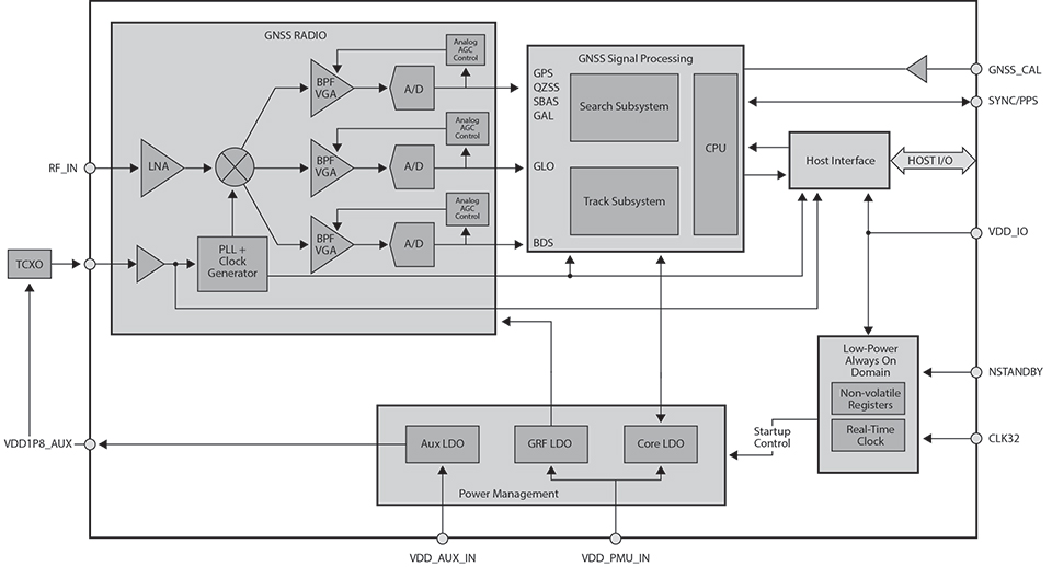
GNSS L1 Signal Down-Conversion
Commercial L1 GNSS signals span a 50 MHz range. It is getting harder for a single antenna to cover the entire bandwidth, but it is possible. The radio input contains three frequency bands of interest, spanning a total of 15 MHz:
BeiDou, at 1561 MHz, is at the low end;
GPS, Galileo, satellite-based augmentation systems (SBAS), and Japan’s Quasi-Zenith Satellite System (QZSS), at 1575 MHz, are in the middle; and
GLONASS, at 1602 MHz, is at the top.
The radio process in the new tri-band receiver described here first amplifies the signal using a low-noise amplifier (LNA) to keep the system noise figure as low as possible. Then it downconverts to an intermediate frequency (IF) and filters the three bands into separate channels. The three bands are then digitized and sampled at the lowest possible sample rate. The sampled bands can be filtered digitally to remove blockers and downconverted to baseband. The baseband samples are buffered by constellations to allow parallel access for searching or tracking on each visible satellite.
All satellites in a code-division multiple access (CDMA) constellation can share baseband buffers, but the frequency-division multiple access (FDMA) constellation, GLONASS, uses a separate buffer for each satellite. This is because the memory and power required to store each satellite in use is less than storing the entire FDMA bandwidth.
Signal Similarities and Differences
All GNSS satellite signals use binary phase-shift keying (BPSK) modulation. The biphase modulation is generated from a high rate pseudorandom noise (PRN) code that is exclusive-ORedwith a low-rate data stream.
The PRN code for all constellations except Galileo is generated from linear feedback shift registers (LFSRs). Galileo’s PRN code is a memory code with a bit-offset carrier BOC(1,1)/BOC(6,1) modulation. All constellations except GLONASS are CDMA. Each satellite in a CDMA constellation is at the same frequency but has a unique PRN code. GLONASS is FDMA. Each visible GLONASS satellite has a unique frequency, but all use the same PRN code.
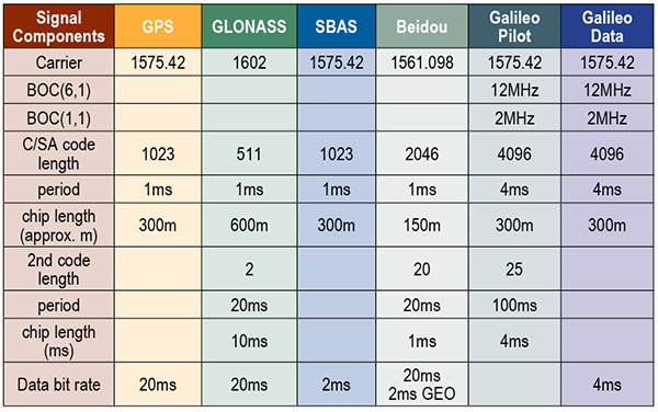
L1 GNSS constellations use four different code lengths: 511, 1023, 2046, and 4092. The code length has a large impact on the power required to detect a signal. Data modulation is different on each constellation. BeiDou data is exclusive-ORed with a secondary code. Galileo has a secondary code-only channel. The highest data or secondary code rate is 1 kHz on BeiDou, and the lowest is 50 Hz on GPS. Table 1 shows a detailed chart with the main signal parameters for all L1 GNSS signals.
Table 1. Parameters for all L1 GNSS signals.
Radio Overview
The radio processing starts with a LNA, which utilizes a 72-nanometer negative metal oxide semiconductor transistor in a cascade configuration, with deliberate capacitive feedback and inductive source degeneration to achieve an excellent noise figure (~1.5 dB system noise figure) while maintaining a good input match. Two external matching components are required to achieve an optimal input match.
Following the LNA is an in-phase/quadrature ring mixer switched-capacitor mixer. With this style of mixer, the LNA output is only connected to one mixer output at a time and, thus, the optimal noise figure is obtained. By switching the output of the LNA from the I+ output and then later to the I– output, a 2:1 voltage gain is achieved. This improves noise figure and eases the noise requirements of the IF amplifier following the mixer, thus reducing power consumption.
The local oscillator for the mixer is derived from a low-power, low phase-noise, phase-locked loop. It has many adjustments, so the circuit can be adapted to a wide variety of reference frequencies and system requirements. It employs a ΔΣ modulator in the feedback loop, allowing for very fine frequency-control resolution.
The complex IF output from the mixer is amplified by a transimpedance section followed by three parallel amplifier/filter/attenuator sections, one for GPS/Galileo/SBAS/QZSS, one for GLONASS, and one for BeiDou. The transimpedance section’s response is close to a simple pole but with a small amount of peaking. Each of the remaining sections is built with a single complex band-pass/band-notch section, followed by real poles and zeroes. Using real poles and zeroes considerably reduces the noise and bandwidth requirements of the amplifiers. The net effect is that the power consumption of the overall IF amplifier section is substantially reduced.
There are three parallel ΔΣ analog-digital converters (ADCs), one for each of the three IF sections. The ΔΣ ADC is a continuous-time, second-order, one-bit ΔΣ ADC, running at a sample rate of 395.75 Msps. The ΔΣ ADC comprises two operational amplifiers, two digital analog converters, and a quantizer. The ΔΣ ADCs are designed in such a way that the quantization noise is lowest not at zero frequency offset (DC), but at the offset frequency of the GNSS signal. The A/D samples are filtered with a third-order cascaded integrator-comb subsampled at 99.44 mega-samples per second. Additional finite impulse response (FIR) filters and subsampling to 33.1 MHz complete the sampling. The combined ΔΣ ADC and digital filtering provide more than 50 dB of dynamic range.
Digital processing at 33.1 MHz includes several filters that remove interference sources from the received radio signal and automatic gain control logic that adjusts the gain of the IF amplifiers to give an optimal signal level. A configurable 20-tap FIR filter is provided for each sample section and can be configured to remove wideband blockers. In addition, each section has eight narrowband, single-pole infinite impulse response filters for removing narrowband blockers.
Figure 1. Radio overview diagram.
Separate Search and Track Blocks
Separate search and track sections are employed to compute correlations between the three sample streams and multiple reference hypotheses. The three sample streams are buffered in memory to allow the search and track sections to process multiple correlations in parallel. Search employs a prime factor fast Fourier transform with a selectable size (1023, 2046, or 4092).
Search correlations are computed by first removing a hypothesis Doppler from a buffered set of samples and then combining a selectable number of code epochs. The filtered samples are translated to the frequency domain, multiplied by the frequency-domain representation of the desired PRN code, and finally translated back to the time domain. This process creates a coherent correlation vector for the entire code. The coherent correlation vector is non-coherently accumulated until the signal-to-noise ratio of the peak exceeds a detection threshold.
Track correlations are computed in the time domain by multiplying a multichip reference code by a set of buffered samples. Typically, the reference code is linearly delayed for N correlations to produce an N-sample coherent correlation vector. The correlation vectors are buffered to allow multiple filters to be processed in parallel. A coprocessor is used to run the filters. The outputs from the coprocessor provide estimates of code phase, Doppler, acceleration, data synchronization, data bits, signal power, and more.
All the buffering and multiple processing sections allow for multiple hypotheses to be tested in parallel. For example, on a tunnel entry, the attenuated signal can continue to be tracked while the search section tries to detect the full-power signal.
Secondary Code Resolution. Several constellations have secondary codes that limit the length of the coherent integration unless the code can be wiped. GLONASS has a 100-Hz Manchester code, BeiDou has a 1-kHz secondary code, and the Galileo Pilot has a 250-Hz secondary code. After the time accuracy drops below 1 millisecond, all of the secondary codes can be wiped in both search and track, so the coherent period can be optimized to maximize sensitivity and minimize measurement error. On a cold start, when time is unknown, it is best to first try to detect with coherent correlations less than the secondary code chip period.
When a signal is detected, the receiver either goes into track and computes correlations with longer coherent periods for multiple time hypotheses or continues in search with a longer coherence period and multiple time hypotheses. The search and track sections allow for either of these choices. For constellations like Galileo, the best choice is to remain in search. For others like BeiDou, it is best to move to track.
Benefits of Multi-GNSS Receivers
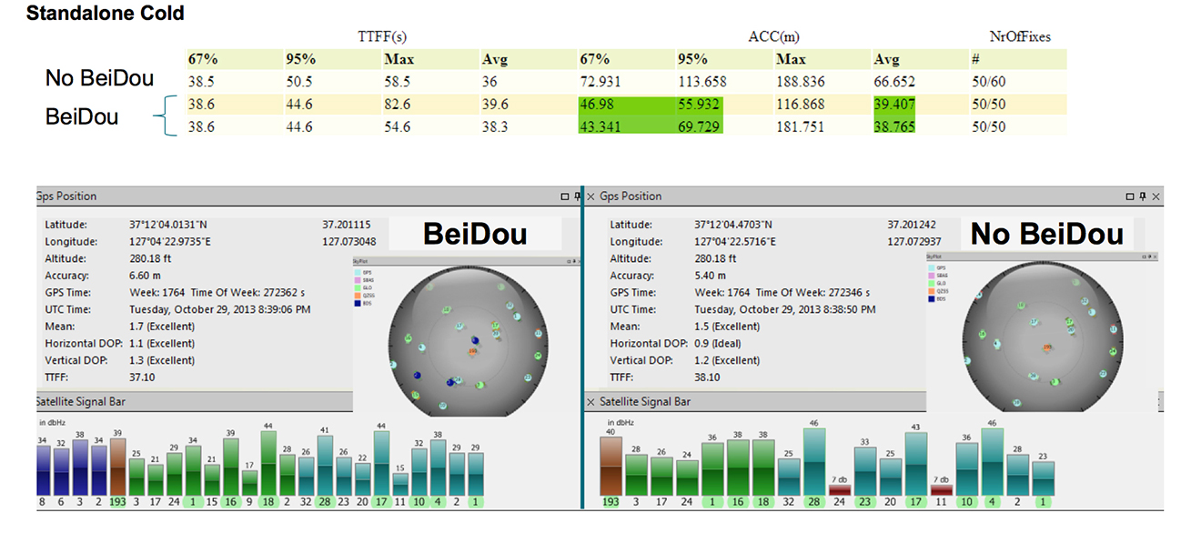
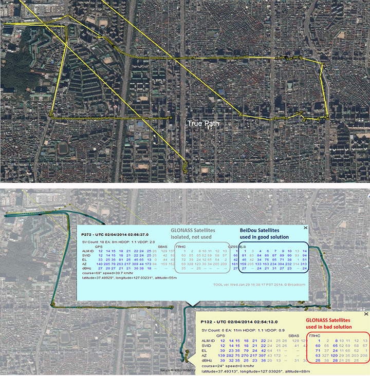
The ability to track all L1 constellations means that even in difficult environments, there are a sufficient number of satellites to produce a navigation solution. As can be seen from field-test results, not only are more satellites tracked, but more satellites with strong signals are tracked. The measurement errors of satellites received with strong signals will be smaller, leading to very low bit-error rates and allowing for a faster ephemeris collection. Field test results confirm that a receiver with BeiDou support achieves faster and more accurate fixes than a receiver without BeiDou support (see Figure 2).
Figure 2. A receiver with BeiDou support achieves faster and more accurate fixes than a receiver without BeiDou support.
In addition to speed and accuracy improvements, more constellations provide a higher reliability. Recently, an upload error in the GLONASS constellation caused otherwise healthy satellites to report orbit errors of several kilometers. GPS/GLONASS-only systems could not completely isolate the faulty satellites. In difficult environments, there are not enough good satellites to isolate the faulty ones. With the addition of BeiDou, the faulty satellites were correctly isolated (Figure 3).
Figure 3. (Top) Seoul, South Korea, third-party GPS/GLONASS-only receiver; (bottom) Broadcom GPS/GLONASS/BeiDou receiver enables isolation of faults.
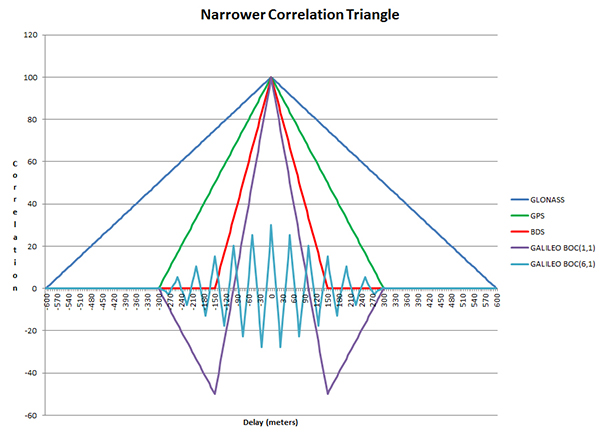
Each constellation adds unique improvements. Narrowing the correlation triangle allows for improved multipath rejection and more accurate pseudorange measurements (Figure 4).
Figure 4. Narrower correlation triangle.
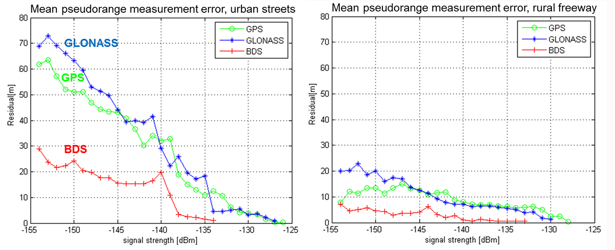
GLONASS, with the slowest code rate, has the broadest correlation triangle. BeiDou, with the highest code rate, has a correlation triangle that is narrower than GPS. The BOC code on Galileo gives the narrowest correlation triangle. Field test results confirm the improved measurements (Figure 5).
GLONASS, the only FDMA constellation, has the least cross-correlation. GPS uses Gold codes to keep the cross-correlations between any of its satellites at a minimum. BeiDou and Galileo have lengthened their codes and added a secondary code to reduce cross-correlations.
Conclusion
Taking advantage of similarities in the L1 GNSS constellations together with careful design choices to minimize size and current consumption has enabled the creation of commercial GNSS system-on-chips that support all current GNSS L1 systems and meet the cost, size, and power requirements of cellular phones. The addition of new constellations like BeiDou and Galileo has significantly improved speed, performance, and reliability.
Acknowledgments
Javier de Salas, Frank van Diggelen, and John Hutson, all of Broadcom.
Manufacturer
The BCM4774 single-chip GNSS location hub for smartphones with Galileo support was designed by Broadcom Corporation.
Charles Norman is a technical director in the GNSS group at Broadcom Corporation. Previously, he worked on GNSS systems at Magnavox, Interstate, SIRF, and RFMD. He holds 39 issued patents on GNSS systems and has an M.A. in mathematics from the University of California-Los Angeles.
Andreas Warloe is a senior technical director in the GNSS group at Broadcom Corporation. He previously worked on GNSS receivers at Magellan, Leica Geosystems, IBM, and RFMD. He holds an M.S. in electrical engineering from the University of Southern California.
Chinese company FOIF is offering a new survey receiver, the A50. FOIF said that with the A50, the company focused on developing a smart design for a receiver to make it lightweight, yet powerful, making it easy to use for fieldwork. Besides Bluetooth, wireless radio, and mobile network (2G and 3G), Wi-Fi feature was added to broaden data communications for GNSS. The A50 is designed to provide excellent performance, with a high-sensitivity GNSS module.
According to FOIF, the A50 has not only sophisticated onboard software, but also optional application programs such as FOIF FieldGenius and Carlson SurvCE, providing multiple field solutions.
The A50’s features include:
Wi-Fi to achieve quick and long distance parameters settings and data transferring;
Tracking of GPS, GLONASS, Galileo, BeiDou satellites on 220 channels;
An industry-standard GNSS engine (Trimble, NovAtel) that can access local CORS;
horizontal real-time accuracy (rms) of 10mm+1ppm, and vertical of 20mm+1ppm;
OLED display with superior brightness and temperature range
Rugged design, with an IP67 rating;
Voice messaging.
RTK(<30km)
H:8 mm + 1 ppm
V:15 mm + 1 ppm
DGPS
H:0.25 m + 1 ppmV:0.50 m + 1 ppm
SBAS
0.5m (initialization time < 10s, initialization reliability > 99.9%)
Eos Positioning Systems has introduced a new line of high-accuracy GNSS receivers for smartphones and tablet computers, including both sub-meter and RTK performance for all mobile platforms: iOS, Android, and Windows.
Eos’s entry-level product, the Arrow Lite, is Bluetooth compatible with all mobile devices.
The Arrow 100 is Eos’s advanced real-time, sub-meter GNSS receiver that utilizes both GPS and GLONASS, and is expandable to Galileo, Beidou and QZSS. It offers superior tracking under tree canopy, around buildings and in rugged terrain, the company said. In addition to supporting SBAS in North/Central America, Europe, Northern Africa, Japan, India and Russia, the Arrow 100 also supports OmniSTAR’s worldwide, real-time sub-meter service.
The most advanced Arrow receiver is the Arrow 200, a dual-frequency, multi-constellation RTK GNSS receiver capable of 1-cm accuracy in real time. The Arrow 200 is an iOS-compatible RTK and OmniSTAR receiver that works with all models of iPads and iPhones via wireless Bluetooth connection. An iOS NTRIP app that allows the user to log into any available RTK network. The Arrow 200 will provide quality RTK performance for years to come because it supports current and future satellite constellations: GPS, GLONASS, Galileo, BeiDou and QZSS, the company said. It also supports OmniSTAR’s G2, XP and HP real-time worldwide decimeter services.
“After spending more than 12 years designing high-accuracy Bluetooth GNSS receivers, I believe Eos has set the new standard for high- accuracy GNSS receivers that work across all mobile platforms, no matter if it’s iOS, Android or Windows,” said Chief Technology Officer Jean-Yves Lauture.
All Arrow receivers employ long-range (1-km) universal Bluetooth connectivity so the user can interface to any brand of smartphone or tablet, whether it’s iOS, Android, or Windows-based. A variable-power Bluetooth implementation allows the Arrow receivers to communicate up to one kilometer from the mobile device.
Arrow receivers have been optimized to run all day on battery power. The battery pack is field-replaceable and rechargeable separately. It contains smart charging logic so expensive battery chargers are not needed.
All Arrow receivers have been designed to meet IP-67 specifications for immersion in water and are completely dust-proof so they will survive in the harshest environments.
The Arrow receiver product line is targeted at high-accuracy applications like GIS, environmental, agriculture, electric/gas/water utilities, surveying, machine control, and federal/state/local government.
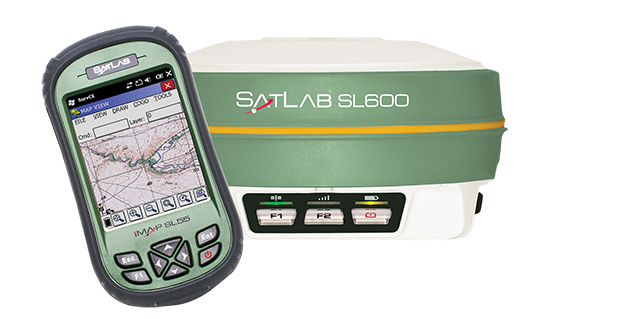
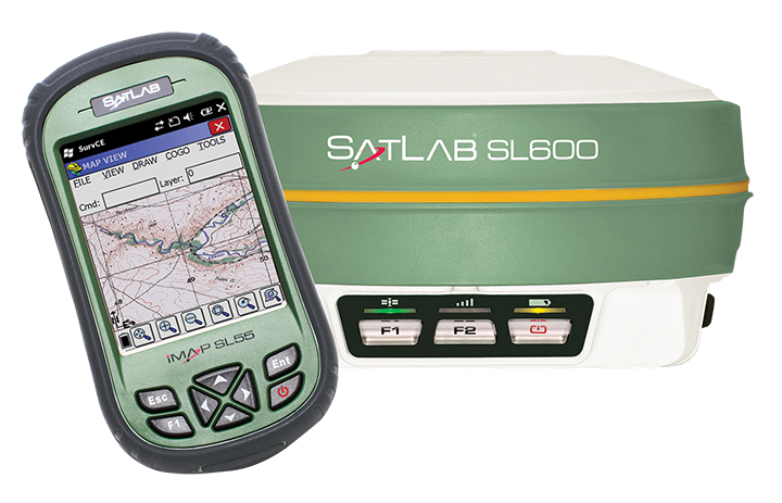
SatLab announced the unit earlier this year as the replacement of its SL500 on-the-pole surveying receiver. After a summer of testing and a premiere showing at InterGeo 2014, held in Berlin in October, SatLab is ready to ship the SL600 to its dealer network and customers.
The new receiver is designed to meet the evolving needs of the surveying market, and is designed for general land, marine and construction applications. At the heart of the rugged unit is a 6G GNSS receiver capable of using all six GNSS satellite networks (GPS, GLONASS, BeiDou, Galileo, QZSS and SBAS), providing reliable operation in demanding conditions, SatLab said.
The SL600 is lightweight at 1.2 kg. Its Xenoy housing holds up well to real-world use, according to test results by SatLab, resistant to 3-meter drops and 2 meters of water submersion. The dual hot swappable batteries provide 18-24 hours of continuous field use, depending on the mode of operation.
The SL600 receiver has a new onboard computer running the LINUX operating system, which ensures easy implementation of new functionalities, often a result of customer-specific requirements. Over time, over-the-air firmware updates will be automatically available, adding new features at no additional charge. Users will be notified by the unit to accept the new firmware updates, or refuse them if they wish to keep their units as is.
The SL600 system is available with various communication capabilities. Cellular 3G and Bluetooth as well USB and RS232 connectivity are standard, and an optional internal 2W Pacific Crest XDL radio is also available. Voice notifications notify the user of issues without the need to watch the status LEDs.
The SL600 system kit includes a compact hard carrying case with the SL55 field controller, which can handle large data files with its high-speed processor and expandable memory. Furthermore, the SL55 has an onboard GPS/GLONASS L1 receiver as well as a GSM modem, which makes the unit a good and rugged companion to use in GIS data collection applications.
As part of the close cooperation between Carlson Software and SatLab Geosolutions AB, the SL600 comes with Carlson SurvCE pre-installed and activated. This ensures an “out of the box” experience for the end customer, SatLab said.
Mauro Colombi, vice president of operations for Stonex, discusses the new S10 GNSS Receiver while at InterGeo 2014, held October 7-9 in Berlin. The S10 features a new generation of smart and open GPS, where a user can install custom applications directly on the receiver.
Hyman Huang of South Surveying & Mapping Instrument Co. talks with GPS World about the company’s new dual-frequency GNSS Receiver and its tablet counterpart while at InterGeo 2014, held October 7-9 in Berlin.
Bruce Carlson, president of Carlson Software, and William “Butch” Herter talk about the company’s new BRx5 GNSS Receiver and Surveyor2 data collector, among others, while at InterGeo 2014, held October 7-9 in Berlin.