Tag: GNSS receiver

  • A Mass-Market Galileo Receiver

    Its Algorithms and Performance

    The authors test three mass-market design drivers on a chip developed expressly for a new role as a combined GPS and Galileo consumer receiver: the time-to-first-fix for different C/N0, for hot, warm, and cold start, and for different constellation combinations; sensitivity in harsh environments, exploiting a simulated land mobile satellite multipath channel and different user dynamics; and power consumption strategies, particularly duty-cycle tracking.

    By Nicola Linty, Paolo Crosta, Philip G. Mattos, and Fabio Pisoni

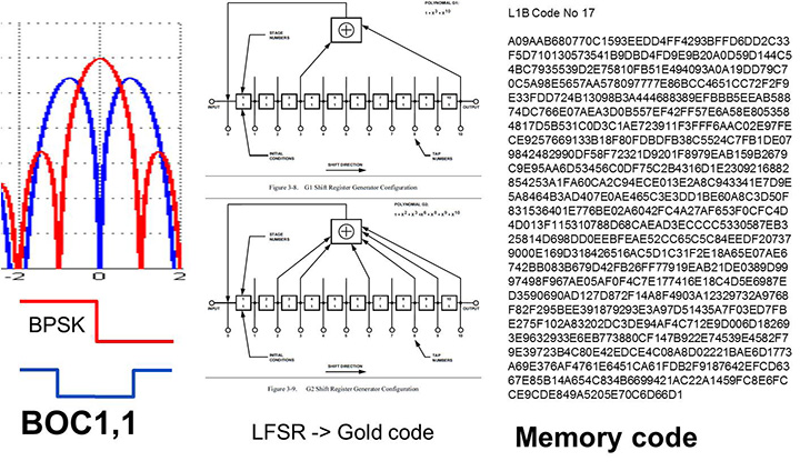
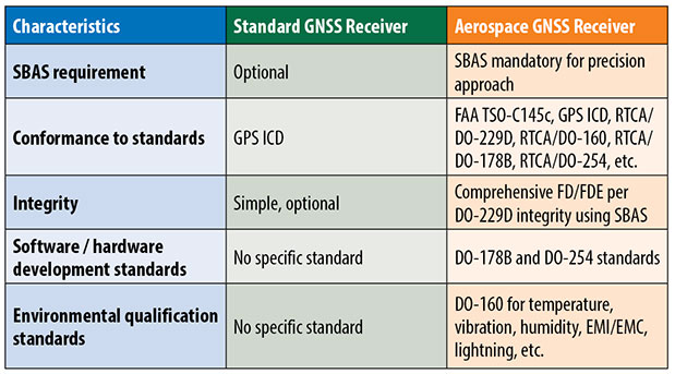
    The two main GNSS receiver market segments, professional high-precision receivers and mass-market/consumer receivers, have very different structure, objectives, features, architecture, and cost. Mass-market receivers are produced in very high volume — hundreds of millions for smartphones and tablets — and sold at a limited price, and in-car GNSS systems represent a market of tens of millions of units per year. The reason for these exploding markets can be found not only in the improvements in electronics and integration, but also in the increasing availability of new GNSS signals. In coming years, with Galileo, QZSS, BeiDou, GPS-L1C, and GLONASS-CDMA all on the way, the silicon manufacturer must continue the path towards the fully flexible multi-constellation mass-market receiver.

    Mass-market receivers feature particular signal processing techniques, different from the acquisition and tracking techniques of standard GNSS receivers, in order to comply with mobile and consumer devices’ resources and requirements. However, a limited documentation is present in the open literature concerning consumer devices’ algorithms and techniques; besides a few papers, all the know-how is protected by patents, held by the main manufacturers, and mainly focused on the GPS L1 C/A signal. We investigate and prove the feasibility of such techniques by semi-analytical and Monte Carlo simulations, outlining the estimators sensitivity and accuracy, and by tests on real Galileo IOV signals.

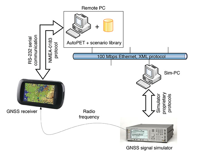
    To understand, analyze, and test this class of algorithms, we implemented a fully software GNSS receiver, running on a personal computer. It can process hardware- and software-simulated GPS L1 C/A and Galileo E1BC signals, as well as real signals, down-converted at intermediate frequency (IF), digitalized and stored in memory by a front-end/bit grabber; it can also output standard receiver parameters: code delay, Doppler frequency, carrier-to-noise power density ratio (C/N0), phase, and navigation message. The software receiver is fully configurable, extremely flexible, and represents an important tool to assess performance and accuracy of selected techniques in different circumstances.

    Code-Delay Estimation

    The code-delay estimation is performed in the software receiver by a parallel correlation unit, giving as output a multi-correlation with a certain chip spacing. This approach presents some advantages, mostly the fact that the number of correlation values that can be provided is thousands of times greater, compared to a standard receiver channel. Use of multiple correlators increases multipath-rejection capabilities, essential features in mass-market receivers, especially for positioning in urban scenarios. The multi-correlation output is exploited to compute the received signal code delay with an open-loop strategy and then to compute the pseudorange.

    In the simulations performed, the multi-correlation has a resolution of 1/10 of a chip, which is equivalent to 30 meters for the signals in question; to increase the estimate accuracy, Whittaker-Shannon interpolation is performed on the equally spaced points of the correlation function belonging to the correlation peak.

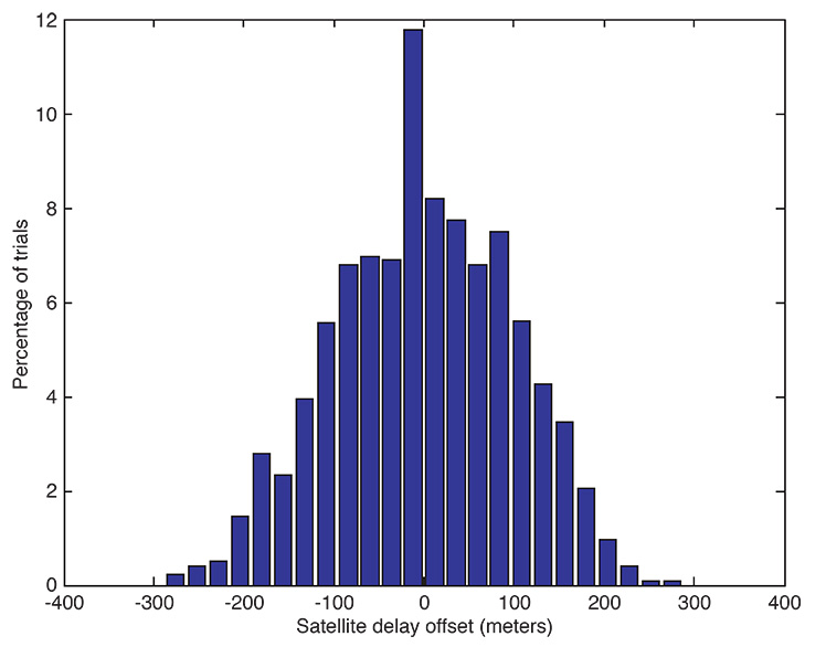
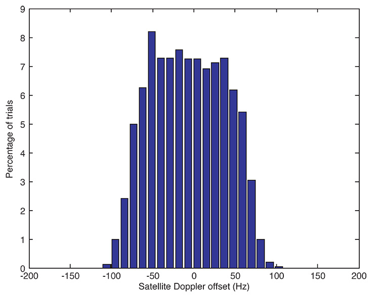
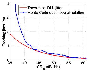
    The code-delay estimate accuracy is reported in Figures 1 and 2. The results are obtained with Monte Carlo simulations on simulated GNSS signals, with sampling frequency equal to 16.3676 MHz. In particular, a GPS L1 C/A signal is considered, affected by constant Doppler frequency equal to zero for the observation period, to avoid the effect of dynamics. The figures show the standard deviation of the code estimation error, that is, the difference between the estimated code delay and the true one, expressed in meters (pseudorange error standard deviation) for different values of C/N0. To evaluate the quality of the results, the theoretical delay locked loop (DLL) tracking jitter is plotted for comparison, as

    Linty-E1

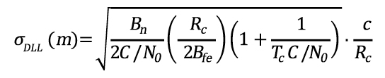
    where Bn is the code loop noise bandwidth, Rc is the chipping rate, Bfe is the single sided front-end bandwidth, Tc is the coherent integration time, and c is the speed of light.

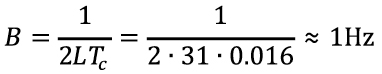
    In the two figures, the red curve shows the theoretical tracking jitter for a DLL, which can be considered as term of comparison for code-delay estimation. To correlate the results, a E-L spacing equal to D = 0.2 chip is chosen, and the code-delay error values of the software receiver simulation are filtered with a moving average filter. By averaging 0.5 seconds of data (for example, L = 31 values spaced 16 milliseconds), an equivalent closed-loop bandwidth of about 1 Hz can be obtained:

    Linty-E2

    In particular, in Figure 1, a coherent integration time equal to 1 millisecond (ms) and 16 non-coherent sums are considered, while in Figure 2 a coherent integration time equal to 4 ms and 16 non-coherent sums, spanning a total time T=64 ms, are considered. In both cases, the software receiver results are extremely good for high C/N0. The code-delay error estimate is slightly higher than its equivalent in the DLL formulation. The open-loop estimation error notably increases in the first case below 40 dB-Hz due to strong outliers, whose probability of occurrence depends on the C/N0. In fact, this effect is smoothed in the second case, where the coherent integration time is four times larger, thus improving the signal-to-noise ratio.

    figure 1 Comparison between code delays estimation accuracy, Tc=1 ms , T=16 ms, B=1 Hz, D=0.2 chip.
    Figure 1. Comparison between code delays estimation accuracy, Tc=1 ms , T=16 ms, B=1 Hz, D=0.2 chip.
    figure 2 Comparison between code delays estimation accuracy, Tc=4 ms, T=64 ms, B=1 Hz, D=0.2 chip.
    Figure 2. Comparison between code delays estimation accuracy, Tc=4 ms, T=64 ms, B=1 Hz, D=0.2 chip.

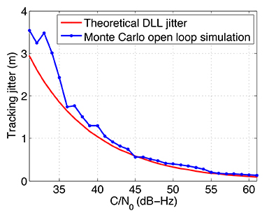
    Nevertheless, the comparison between open loop multi-correlation approach and closed loop DLL is difficult and approximate, because the parameters involved are different and the results are only qualitative.

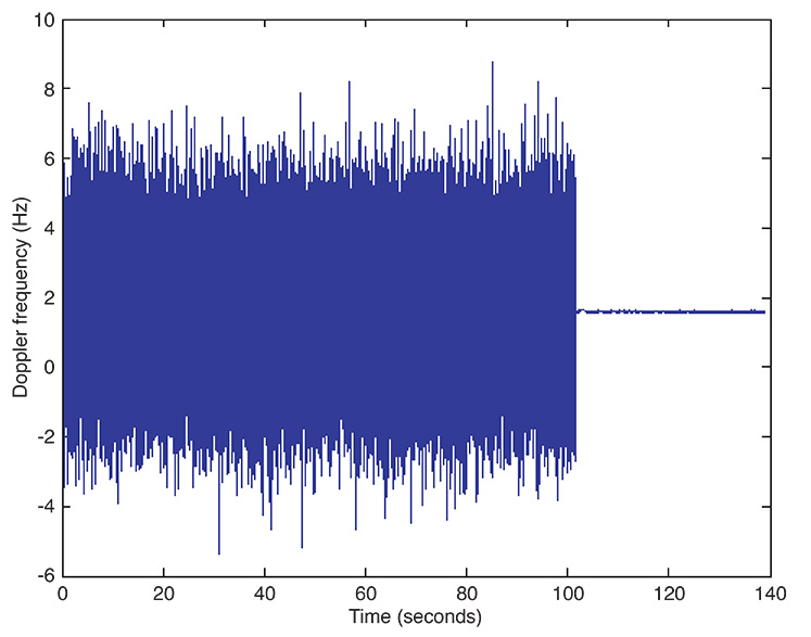
    Doppler Frequency Estimation

    In the particular case of the software receiver developed here, the residual Doppler frequency affecting the GNSS signal is estimated by means of a maximum likelihood estimator (MLE) on a snapshot of samples, exploiting open-loop strategy. In fact, despite the higher standard deviation of the frequency error (jitter), open-loop processing offers improved tracking sensitivity, higher tracking robustness against fading and interference, and better stability when increasing the coherent integration time. In addition, the open-loop approach does not require the design of loop filters, avoiding problems with loop stability. A certain number of successive correlator values, computed in the multiple correlations block, are combined in a fast Fourier transform (FFT) and interpolated.

    Figure 3 shows the root mean square error (RMSE) of the frequency estimate versus signal
    C/N0, obtained collecting 16 coherent accumulations of 4 ms of a Galileo E1B signal, then computing a 16 points FFT spanning a time interval of 64 ms, and finally refining the result with an interpolation technique. Three different curves are shown, corresponding respectively to:

    • the RMSE derived from simulations, carried out with GNSS data simulated with the N-FUELS signal generator;
    • a semi-analytical estimation, exploiting the same algorithm;
    • the Cramer-Rao lower bound (CRLB) for frequency estimation, shown as

    Linty-E3

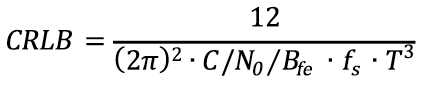
    where fs is the sampling frequency.

    Figure 3. Doppler frequency estimate RMSE versus C/N0 in super-high resolution with T=64 ms, comparison between theoretical and simulated results.
    Figure 3. Doppler frequency estimate RMSE versus C/N0 in super-high resolution with T=64 ms, comparison between theoretical and simulated results.

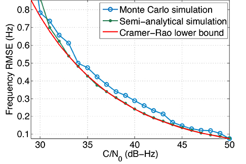
    A well-known drawback is the so-called threshold effect. Below a certain C/N0, the frequency estimate computed with MLE suffers from an error, and the RMSE increases with respect to the CRLB.

    Mass-Market Design Drivers

    Once we have analyzed the features of some mass-market algorithms with a software receiver, we can move toward the performance of a real mass-market device, to compare results and confirm improvements brought by the new Galileo signals, so far mainly known from a theoretical point of view.

    A recent survey identified three main drivers in the design of a mass-market receiver, coming directly from user needs, and solvable in different ways.

    Time-to-first-fix (TTFF) corresponds to how fast a position, velocity, and time (PVT) solution is available after the receiver is powered on, that is, the time that a receiver takes to acquire and track a minimum of four satellites, and to obtain the necessary information from the demodulated navigation data bits or from other sources.

    Capability in hostile environments, for example while crossing an urban canyon or when hiking in a forest, is measured in terms of sensitivity. It can be verified by decreasing the received signal strength and/or adding multipath models.

    Power consumption of the device. GNSS chipset is in general very demanding and can produce a not-negligible battery drain.

    We analyzed these three drivers with a commercial mass-market receiver and with the software receiver.

    Open-Sky TTFF Analysis

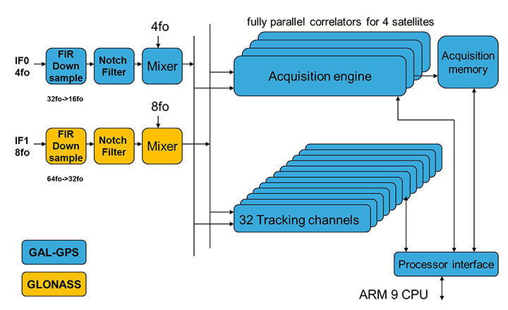
    TTFF depends on the architecture of the receiver, for example the number of correlators or the acquisition strategy, on the availability of assistance data, such as rough receiver position and time or space vehicles’ (SV) ephemeris data, and on the broadcast navigation message structure. Some receivers, like the one used here for testing, embed an acquisition engine that can be activated on request and assures a low acquisition time; moreover, they implement ephemeris extension. In contrast, other consumer receiver manufacturers exploit a baseband-configurable processing unit, similar to the one implemented in the software receiver, with thousands of parallel correlators generating a multi-correlator output with configurable spacing, depending on the accuracy required. By selecting an appropriate number of correlators, depending on the available assistance data and on the accuracy required, the TTFF consequently varies.

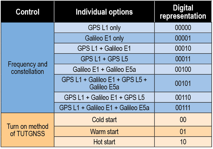
    We assessed the performance of the receiver under test for different C/N0, for hot, warm, and cold start, and for different constellation combinations, exploiting hardware-simulated GNSS data. Good results are achieved, especially when introducing Galileo signals.

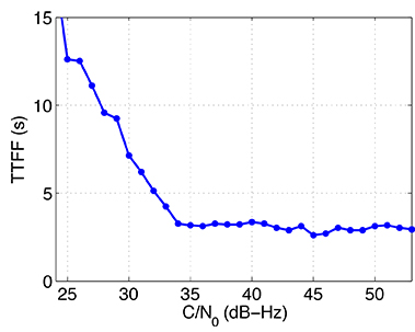
    Figure 4 reports the hot-start TTFF for different C/N0 values in the range 25–53 dB-Hz, computed using the receiver. The receiver, connected to a signal generator, is configured in dual-constellation mode (GPS and Galileo) and carries out 40 TTFF trials, with a random delay between 15 and 45 seconds. In a standard additive white Gaussian noise (AWGN) channel and in hot-start conditions, the results mainly depend on the acquisition strategy and on the receiver availability of correlators and acquisition engines. In an ideal case with open-sky conditions and variable C/N0, the introduction of a second constellation only slightly improves the TTFF performance; this result cannot be generalized since it mainly depends on the acquisition threshold of the receiver, which can change using signals of different constellations. In real-world conditions, the situation can vary.

    figure 4 Hot start TTFF for Galileo+GPS configuration versus C/N0 using the test receiver.
    Figure 4. Hot start TTFF for Galileo+GPS configuration versus C/N0 using the test receiver.

    Cold Start. Secondly, we analyze TTFF differences due to the different structure of GPS and Galileo navigation messages. The I/NAV message of the Galileo E1 signal and the data broadcast by GPS L1 C/A signals contain data related to satellite clock, ephemeris, and GNSS time: parameters relevant to the position fix since they describe the position of the satellite in its orbit, its clock error, and the transmission time of the received message.

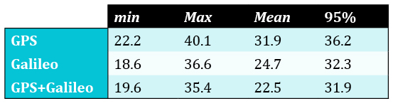
    Table 1 shows some results in the particular case of cold start, with an ideal open-sky AWGN scenario. The TTFF is significantly lower when using Galileo satellites: while the mean TTFF when tracking only GPS satellites is equal to about 31.9 seconds (s), it decreases to 24.7 s when considering only Galileo satellites, and to 22.5 s in the case of dual constellation. Similarly, the minimum and maximum TTFF values are lower when tracking Galileo satellites. The 95 percent probability values confirm the theoretical expectations. Again, in the ideal case with open-sky conditions, the results with two constellations are quite similar to the performance of the signal with faster TTFF. However, in non-ideal conditions, use of multiple constellations represents a big advantage and underlines the importance of developing at least dual-constellation mass-market receivers.

    table 1 Comparison between TTFF (in seconds) in cold start for different constellation combinations.
    Table 1. Comparison between TTFF (in seconds) in cold start for different constellation combinations.

    Furthermore, it is interesting to analyze in more detail the case of a GPS and Galileo joint solution. GPS and Galileo system times are not synchronized, but differ by a small quantity, denoted as the GPS-Galileo Time Offset (GGTO). When computing a PVT solution with mixed signals, three solutions are possible: to estimate it as a fifth unknown, to read it from the navigation message, or to use pre-computed value. In the first case it is not necessary to rely on the information contained in the navigation message, eventually reducing the TTFF. However, five satellites are required to solve the five unknowns, and this is not always the case in urban scenarios or harsh environments, as will be proved below. On the contrary, in the second case, it is necessary to obtain the GGTO information from the navigation message, and since it appears only once every 30 seconds, in the worst case it is necessary to correctly demodulate 30 seconds of data. Both approaches show benefits and disadvantages, depending on the environment. The receiver under test exploits the second solution: in this case, it is possible to see an increase in the average TTFF when using a combination of GPS and Galileo, due to the demodulation of more sub-frames of the broadcast message.

    Sensitivity: Performance in Harsh Environments

    Harsh environment is the general term used to describe those scenarios in which open sky and ideal propagation conditions are not fulfilled. It can include urban canyons, where the presence of high buildings limits the SV visibility and introduces multipath; denied environments, where unintentional interference may create errors in the processing; or sites where shadowing of line-of-sight (LoS) path is present, for example due to trees, buildings, and tunnels. In these situations it is necessary to pay particular attention to the signal-processing stage; performance is in general reduced up to the case in which the receiver is not able to compute a fix.

    A first attempt to model such an environment has been introduced in the 3GPP standard together with the definition of A-GNSS minimum performance requirements for user equipment supporting other A-GNSSs than GPS L1 C/A, or multiple A-GNSSs which may or may not include GPS L1 C/A. The standard test cases support up to three different constellations; in dual-constellation case it foresees three satellites in view for each constellation with a horizontal dilution of precision (HDOP) ranging from 1.4 to 2.1.

    To perform TTFF and sensitivity tests applying the 3GPP standard test case, we configured a GNSS simulator scenario with the following characteristics, starting from the nominal constellation:

    • Six SVs: three GPS (with PRN 6,7, 21) and three Galileo (with code number 4, 11, 23);
    • HDOP in the range 1.4 – 2.1;
    • nominal power as per corresponding SIS-ICD;
    • user motion, with a heading direction towards 90° azimuth, at a constant speed of 5 kilometers/hour (km/h).

    In addition to limiting the number of satellites, we introduced a narrowband multipath model. The multi-SV two-states land mobile satellite (LMS) model simulator generated fading time series representative of an urban environment. The model includes two states:

    • a good state, corresponding to LOS condition or light shadowing;
    • a bad state, corresponding to heavy shadowing/blockage.

    Within each state, a Loo-distributed fading signal is assumed. It includes a slow fading component (lognormal fading) corresponding to varying shadowing conditions of the direct signal, and a fast fading component due to multipath effects. In particular, the last version of the two-state LMS simulator is able to generate different but correlated fading for each single SV, according to its elevation and azimuth angle with respect to the user position: the angular separation within satellites is crucial, since it affects the correlation of the received signals. This approach is based on a master–slave concept, where the state transitions of several slave satellites are modeled according to their correlation with one master satellite, while neglecting the correlation between the slave satellites. The nuisances generated are then imported in the simulator scenario, to timely control phase and amplitude of each simulator channel. Using this LMS scenario, the receiver’s performance in harsh environments has been then verified with acquisition (TTFF) and tracking tests.

    The TTFF was estimated with about 50 tests, in hot, warm, and cold start, first using both GPS and Galileo satellites, and then using only one constellation. In the second case only the 2D fix is considered, since, according to the scenario described, at maximum three satellites are in view. Table 2 reports the results for the dual-constellation case: in hot start the average TTFF is about 8 s, and it increases to 36 s and 105 s respectively for the warm and cold cases. Clearly the results are much worse than in the case reported earlier of full open-sky AWGN conditions. In this scenario only six satellites are available at maximum; moreover, the presence of multipath and fading affects the results, and they exhibit a larger variance, because of the varying conditions of the scenario.

    Table 2. TTFF (in seconds) exploiting GPS and Galileo constellations in harsh environments.
    Table 2. TTFF (in seconds) exploiting GPS and Galileo constellations in harsh environments.

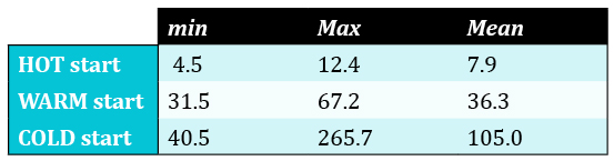
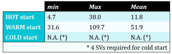
    Table 3 shows similar results, but for the GPS-only case. In this case the receiver was configured to track only GPS satellites. The mean TTFF increases both in the hot and in the warm case, whereas in cold start it is not possible compute a 2D fix with only three satellites; the ambiguity of the solution cannot be solved if an approximate position solution is not available. It may seem unfair to compare a scenario with three satellites and one with six satellites. However, it can be assumed that this is representative of what happens in limited-visibility conditions, where a second constellation theoretically doubles the number of satellites in view.

    Table 3. TTFF (in seconds) exploiting only GPS constellations in harsh environments.
    Table 3. TTFF (in seconds) exploiting only GPS constellations in harsh environments.

    The results confirm the benefits of dual-constellation mass-market receivers in harsh environments where the number of satellites in view can be very low. Making use of the full constellation of Galileo satellites will allow mass-market receivers to substantially increase performances in these scenarios.

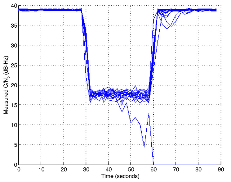
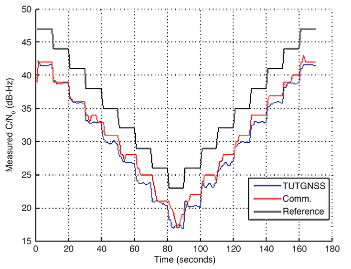
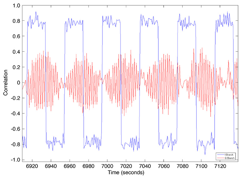
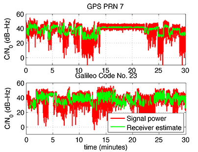
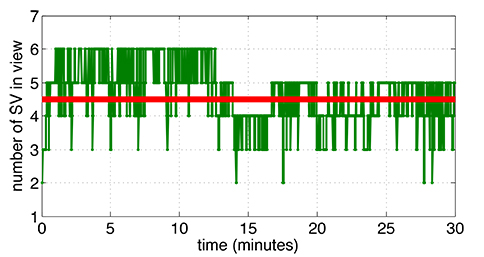
    Tracking.We carried out a 30-minute tracking test with both the receiver and the software receiver model. Both were able to acquire the six satellites and to track them, even with some losses of lock (LoLs) due to fading and multipath reflections. Figure 5 shows the number of satellites in tracking state in the receiver at every second, while Figure 6 shows the HDOP as computed by the receiver. When all six satellites are in tracking state, the HDOP lies in the range 1.4 – 2.1, as defined in the simulation scenario; on the contrary, as expected, in correspondence with a LoL it increases.

    Figure 6. HDOP computed by the test receiver in the Multi-SV LMS simulation.
    Figure 6. HDOP computed by the test receiver in the Multi-SV LMS simulation.

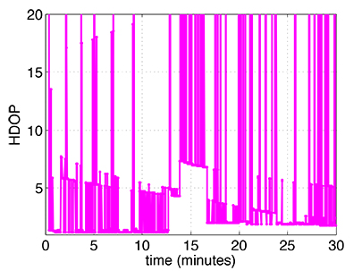
    Figure 7 compares the signal power generated by the simulator and the power estimated by the receiver, in the case of GPS PRN 7 and Galileo code number 23. This proves the tracking capability of the receiver also for high sensitivity. To deal with low-power signals, the integration time is extended both for GPS and for Galileo, using the pilot tracking mode in the latter case.

    Figure 7. C/N0 estimate computed by the receiver in harsh environments and compared with the signal power.
    Figure 7. C/N0 estimate computed by the receiver in harsh environments and compared with the signal power.

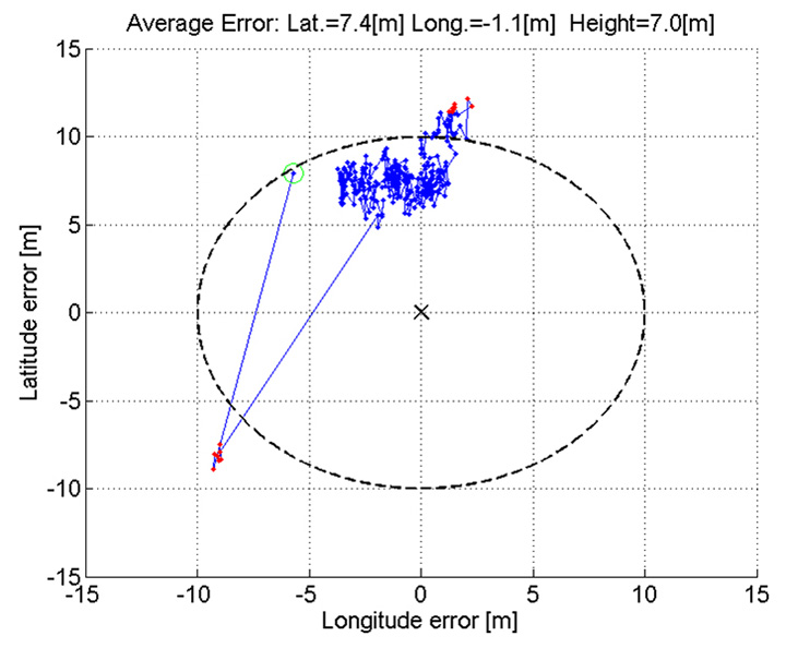
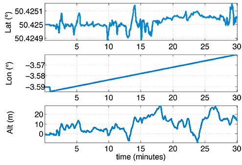
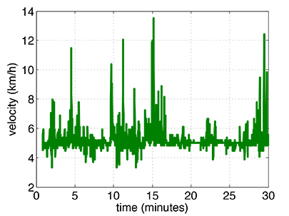
    Figures 8 and 9 show respectively the position and the velocity solution. In the first case latitude, longitude, and altitude are plotted, while in the second case the receiver speed estimate in km/h is reported.

    Figure 8. Test receiver position solution in LMS scenario.
    Figure 8. Test receiver position solution in LMS scenario.
    Figure 9. Test receiver velocity solution in LMS scenario.
    Figure 9. Test receiver velocity solution in LMS scenario.

    In this framework it is possible to evaluate the advantages and disadvantages of using the broadcast GGTO when computing a mixed GPS and Galileo position. When the LMS channel conditions are good, all six SVs in view are in tracking state, as shown in Figure 5. However, when the fading becomes important, the number is reduced to only two satellites. If the receiver is designed to extract the GGTO from the navigation message, then a PVT solution is possible also when only four satellites are in tracking state, that is for 90 percent of the time in this specific case. On the contrary, if the GGTO has to be estimated, one more satellite is required, and this condition is satisfied only 57 percent of the time, strongly reducing the probability of having a fix. Nevertheless, estimating the GGTO requires the correct demodulation of the navigation message, and this is possible only if the signal is good enough for a sufficient time.

    figure 5 Number of satellites tracked by the test receiver in the Multi-SV LMS simulation.
    Figure 5. Number of satellites tracked by the test receiver in the Multi-SV LMS simulation.

    Power-Saving Architectures

    The final driver for mass-market receivers design is represented by power consumption. Particularly for chips suited for portable devices running on batteries, power drain represents one of the most important design criteria. To reduce at maximum the power consumption, chip manufacturers have adopted various solutions. Most are based on the concept that, contrarily to a classic GNSS receiver, a mass-market receiver is not required to constantly compute a PVT solution. In fact, most of the time, GNSS chipsets for consumer devices are only required to keep updated information on approximate time and position and to download clock corrections and ephemeris data with a proper time rate, depending on the navigation message type and the adopted extended ephemeris algorithm. Then, when asked, the receiver can quickly provide a position fix. By reducing the computational load of the device during waiting mode, power consumption is reduced proportionally.

    To better understand advantages and disadvantages of power saving techniques, some of them have been studied and analyzed in detail. In particular, the algorithm implemented in the software receiver model is based on two different receiver states: an active state, in which all receiver parts are activated, as in a standard receiver, and a sleep state, where the receiver is not operating at all. In the sleep state, the GNSS RF module, GNSS baseband, and digital signal processor core are all switched off. By similarity to a square wave, these types of tracking algorithms are also called duty-cycle (DC) algorithms. Exploiting the software approach’s flexibility, we can test the effect of two important design parameters:

    • sleep period length;
    • minimum active period length.

    Their setting is not trivial and depends on the channel conditions, on the signal strength, on the number of satellites in view, on the user dynamics, and finally on the required accuracy.

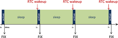
    In the software receiver simulations performed, the active mode length is fixed to 64 ms: the receiver collects 16 correlation values with coherent integration time equal to 4 ms, to perform frequency estimation as described above. Then it switches to sleep state for 936 ms, until a real-time clock (RTC) wake-up initiates the next full-power state. In this way a fix is available at the rate of 1 s, as summarized in Figure 10. However, there are some situations where the receiver may stay in full-power mode, for example during the initialization phase, to collect important data from the navigation message, such as the ephemeris, and to perform RTC calibration.

    Figure 10. Duty cycle tracking pattern in the software receiver simulations.
    Figure 10. Duty cycle tracking pattern in the software receiver simulations.

    There are benefits of using this approach coupled to Galileo signals: the main impact is the usage of the pilot codes. Indeed, a longer integration time allows reducing the active period length, which most impacts the total power consumption, being usually performed at higher repetition rate.

    Some simulations were carried out to assess the performance of DC algorithms in the software receiver. While in hardware implementations the direct benefit is the power computation, in a software implementation it is not possible to see such an improvement. The reduced power demand is translated into a shorter processing time for each single-processing channel. The DC approach can facilitate the implementation of a real-time or quasi-real-time software receiver.

    The main drawback of using techniques based on DC tracking is the decrease of the rate of observables and PVT solution. However, this depends on the application; for some, a solution every second is more than enough.

    Real-Signal Results

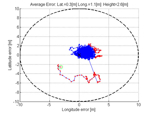
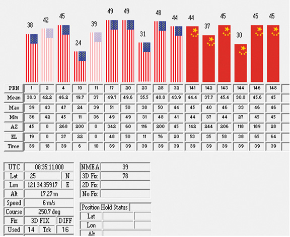
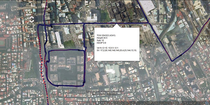
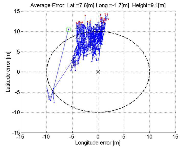
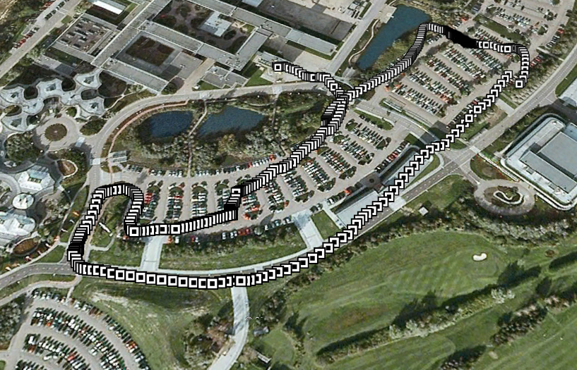
    On March 12, 2013, for the first time  the four Galileo IOV satellites were broadcasting a valid navigation message at the same time. From 9:02 CET, all the satellites were visible at ESTEC premises, and the first position fix of latitude, longitude, and altitude took place at the TEC Navigation Laboratory at ESTEC (ESA) in Noordwijk, the Netherlands. At the same time, we were able to acquire, track, and compute one of the first Galileo-only mobile navigation solutions, using the receiver under test. Thanks to its small size and portability, it was installed on a mobile test platform, embedded in ESA’s Telecommunications and Navigation Testbed vehicle. Using a network connection, we could follow, from the Navigation Lab, the real-time position of the van moving around ESTEC.

    Figure 11 shows the van’s track, obtained by post processing NMEA data stored by the receiver evaluation board. The accuracy achieved in these tests met all the theoretical expectations, taking into account the limited infrastructure deployed so far. In addition, the results obtained with the receiver have to be considered preliminary, since its firmware supporting Galileo was in an initial test phase (for example, absence of a proper ionospheric model, E1B-only tracking).

    Figure 11. Galileo-only mobile fix, computed on March 12, 2013.
    Figure 11. Galileo-only mobile fix, computed on March 12, 2013.

    Conclusions

    Analysis of a receiver’s test results confirms the theoretical benefits of Galileo OS signals concerning TTFF and sensitivity. Future work will include the evolution of the software receiver model and a detailed analysis of power-saving tracking capabilities, with a comparison of duty-cycle tracking techniques in open loop and in closed loop.

    Acknowledgments

    This article reflects solely the authors’ views and by no means represents official European Space Agency or Galileo views. The article is based on a paper first presented at ION GNSS+ 2013. Research and test campaigns related to this work took place in the framework of the ESA Education PRESTIGE programme, thanks to the facilities provided by the ESA TEC-ETN section. The LMS multipath channel model was developed in the frame of the MiLADY project, funded by the ARTES5.1 Programme of the ESA Telecommunications and Integrated Applications Directorate.

    Manufacturers

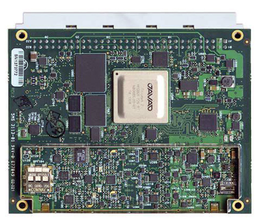
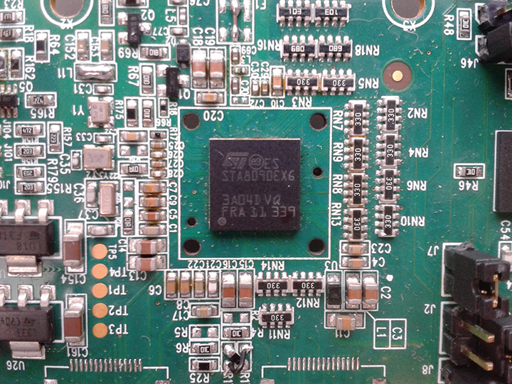
    The tests described here used the STMicroelectronics Teseo II receiver chipset and a Spirent signal simulator.


    Nicola Linty is a Ph.D. student in electronics and telecommunications at Politecnico di Torino. In 2013 he held an internship at the European Space Research and Technology Centre of ESA.

    Paolo Crosta is a radio navigation system engineer at the ESA TEC Directorate where he provides support to the EGNOS and Galileo programs. He received a MSc degree in telecommunications engineering from the University of Pisa.

    Philip G. Mattos received an external Ph.D. on his GPS work from Bristol University. He leads the STMicroelectronics team on L1C and BeiDou implementation, and the creation of totally generic hardware that can handle even future unknown systems.

    Fabio Pisoni has been with the GNSS System Team at STMicroelectronics since 2009. He received a master’s degree in electronics from Politecnico di Milano, Italy.

  • Innovation: A PET Project from Finland

    Innovation: A PET Project from Finland

    Automating GNSS Receiver Testing

    By Sarang Thombre, Jussi Raasakka, Tommi Paakki, Francescantonio Della Rosa, Mikko Valkama, Laura Ruotsalainen, Heidi Kuusniemi, and Jari Nurmi

    GPS World photo
    INNOVATION INSIGHTS by Richard Langley

    WE HAVE A CAT. My wife and I do, that is. One with a voracious appetite. She likes to be fed on demand, even at the most inopportune times. Like three o’clock in the morning. No, it doesn’t help to close the bedroom door. Her squeaking (yes, some cats squeak) still wakes us up. I was designated as the one to get up in the night to feed her. Sometimes twice. Each night, every night. That got tiresome (literally) very quickly. Automation came to the rescue. We now have a microprocessor-controlled cat feeder, which rotates food compartments into the feeding position at pre-programmed times. Just fill up one or two of the compartments with “crunchies” before retiring, set the activation time to 3:00 a.m., say, and no more middle-of-the-night squeaking interrupting blissful sleep.

    This is just one example of how automation — machines replacing (or supplementing) human activity to perform repetitive, difficult, undesirable, or even humanly-impossible tasks — can affect (and benefit) our everyday lives.

    As noted on Wikipedia, two common types of automation are ones that involve feedback control, which is usually continuous and involves making measurements using one or more sensors and computing adjustments to keep the measured variables within a set range, and those that involve sequence control, in which a programmed sequence of discrete operations is performed, often based on system logic. An aircraft autopilot is an example of the former while our cat-feeding machine is an example of the latter. Some systems, such as Earth-orbiting satellites, can involve both types.

    Automation applications range from the (now) mundane (such as point-and-shoot cameras, smart phones, home control, and factory assembly lines) to the (now) exotic (such as robots to assist the elderly and the infirm and robots to explore space). Laboratories have also benefited from increasing automation, making rapid clinical and analytical testing, for example, possible.

    The testing of GNSS receivers can also benefit from automation. This work typically requires the active participation of humans to initiate, control, monitor, and terminate test cases. These manual operations are often inefficient and inaccurate, rendering the test results unreliable.  Furthermore, accessing the internal signals of a receiver at different stages of processing is necessary to pinpoint the exact location of any anomalies. Using traditional black-box testing techniques, it is only possible to test the final outputs of a receiver. In this month’s column, we take a look at an automated test bench for analyzing the overall performance of multi-frequency, multi-constellation GNSS receivers. The system includes a data-capture tool to extract internal process information and controlling software, called the Automated Performance Evaluation Tool or AutoPET, which is able to communicate between all modules of the system for hands-free, one-button-click testing of GNSS receivers. Would my cat appreciate the benefit? Likely not, but GNSS engineers and scientists certainly will.

    “Innovation” is a regular feature that discusses advances in GPS technology and its applications as well as the fundamentals of GPS positioning. The column is coordinated by Richard Langley of the Department of Geodesy and Geomatics Engineering, University of New Brunswick. He welcomes comments and topic ideas.


    The prototype GNSS receiver developed at the Department of Electronics and Communications Engineering of Tampere University of Technology (TUT), called TUTGNSS, is now in the performance-testing phase. TUTGNSS is a GPS L1/L5 + Galileo E1/E5a dual-frequency dual-constellation receiver jointly developed by TUT and its international partners under two European Union Framework Programme research grants.

    During the manual testing of the receiver, it was noticed that the results were often contaminated with errors due to imprecise time-keeping and inconsistent test environments.

    It was also strenuous and time consuming to perform repetitive tests over multiple iterations, with decreasing personnel efficiency as the number of iterations increased. The aforementioned problems led to the results being deemed unreliable and unrepeatable. There was thus a need to innovate and automate the testing process and environment. In addition, there was also the need to study the signals as they flowed through the internal signal processing chain, so that the exact location of anomalies could be detected.

    Currently, few solutions are available in the commercial and academic domains, which can perform end-to-end fully automated, yet customizable testing of GNSS receivers. A couple of commercial testing tools were recently unveiled, which claim to perform similar automated testing of GNSS receivers. However, these are not fully customizable by the end-user, having the limitation that they can be used only with their parent company’s proprietary signal simulators. Other commercial automated testing tools are available nowadays. However, they are targeted towards electronic systems other than GNSS receivers. It was due to these reasons that we decided to implement an in-house solution. Consequently, we devised the Automated Performance Evaluation Tool (AutoPET), along with a data capture tool.

    AutoPET is implemented completely in software (Qt, with C++) and communicates with the receiver under test (RUT) via RS-232 and a National Marine Electronics Association (NMEA) protocol and with a commercial GNSS signal simulator via an RS-232 link. It handles the GNSS test cases with user-defined iterations and other system settings. AutoPET has already been used for making test runs on the TUTGNSS receiver with positive results. It is possible to initiate the overall testing of the receiver with a single button-click and the results are stored in the computer without any human intervention. Test scenarios currently included in the tool’s library are: time-to-first-fix (TTFF), position accuracy, acquisition sensitivity, tracking sensitivity, and reacquisition time. By changing the scenarios in this library, the tool can be used with different simulator models. Another innovative aspect of AutoPET is that it uses multi-threading to perform the receiver testing. Multiple software processing threads are necessary to keep track of the receiver operations and simulator feeds simultaneously, so that an appropriate interrupt can be generated when the receiver has performed the desired operation. This feature is explained in further detail later on.

    Data Capture Tool (dCAP) is a hybrid (software-controlled hardware) entity capable of extracting the user-defined internal process data from the different modules (acquisition, tracking, bit decoding, and so on) of the GNSS RUT and stores it in a computer via a 100-Mbps Ethernet link. The dCAP hardware is independent of the receiver module (although implemented on the same softcore) and operates through minimal interference with the receiver operation. This data can then be post-processed to monitor and record the behavior of the receiver and to investigate any anomalies in its intermediate stages. An experimental version of dCAP has already been used to monitor the carrier-to-noise-density ratio (C/N0), carrier Doppler, and code delay from the internal tracking channels, and the raw GNSS signals in I/Q format entering the baseband processing unit (BPU) of the TUTGNSS receiver from its radio front end.

    The benefits of AutoPET over state-of-art approaches are that it is portable (software platform independent), easy to use, suitable for testing most receivers using a variety of simulators (provided each of them can communicate with the outside world using some form of communication protocol), and its operational parameters are easy to modify through an external configuration file. dCAP is designed specifically for the TUTGNSS receiver; however, it can be easily replicated for most experimental embedded system receivers. Once implemented, dCAP offers a clear view of the internal operation of the receiver by accessing intermediate signals between the input and output terminals. The speed and size of data capture are limited only by the type of Ethernet connection and the size of the internal and external memories. Additional details of AutoPET and dCAP are provided in the next two sections of this article, while the third section describes the application of these tools in testing the GPS L1 operation of the TUTGNSS receiver.

    Automated Performance Evaluation Tool

    AutoPET is a software program developed using the Qt platform and the C++ language, which communicates between the GNSS receiver, signal simulator, and its associated computer through a remote PC that houses AutoPET. The set-up is shown in FIGURE 1. This figure also denotes the different communication protocols used between the different modules.

    FIGURE 1. Block schematic of the AutoPET assembly.
    FIGURE 1. Block schematic of the AutoPET assembly.

    At the center is the GNSS receiver, which accepts RF signals from the GNSS signal simulator. These signals represent signals from the sky in accordance with the scenario loaded in the simulator, and therefore represent unidirectional communication. On the other hand, the receiver communicates with the remote PC housing AutoPET using the NMEA-0183 protocol. This is bidirectional communication, as the receiver continuously updates its status via NMEA messages to AutoPET and, in turn, AutoPET sends a response/control command to the receiver. The receiver sends the $GPGGA NMEA message every second, and through reading this message, AutoPET can determine the current status (acquisition, tracking, position fix, and so on) of the receiver.

    The TUTGNSS receiver has the capability to perform a cold start to initiate the next test iteration when commanded by AutoPET. For this purpose, we have designed a simple custom message string, which can be identified by the TUTGNSS receiver as a cold-start command. In response, the receiver sends a custom NMEA message, $GPTXT, which identifies that it has successfully performed a cold start. Performing a cold start involves erasing all a priori navigation-related information from the receiver memory. This includes erasing the ephemeris, almanac, and timing information, and ensuring that all satellite tracking is lost.

    AutoPET communicates with the GNSS signal simulator through its controlling computer, called the Sim-PC (which runs the control software for the simulator). This communication is bidirectional using a 100-Mbps Ethernet link. The AutoPET library holds the scenario files, through which it remotely controls the simulator. In turn, the Sim-PC returns responses or error messages in the form of Extensible Markup Language (XML) strings to the AutoPET. The communication between the Sim-PC and the simulator is through its proprietary protocols.

    AutoPET makes extensive use of multi-threading. The receiver, AutoPET, and the simulator function autonomously of each other and hence are independently controlled using their own processing threads running in parallel. Examples of some processing threads are:

    • Thread 1 – monitors the receiver operation through the received NMEA messages. This thread is responsible for identifying, for example, if the receiver achieves a position fix or if it performs a successful cold start.
    • Thread 2 – monitors the simulator through the received XML error messages and response messages from the Sim-PC. It is responsible for identifying, for example, if the simulator scenario is successfully set up or if the satellite signals are turned on and off when demanded by the test case.
    • Thread 3 – monitors the internal operation of AutoPET itself to check, for example, if a timer has expired or if the user performs any operation on the GUI during the progress of a test.

    Each thread generates an internal software interrupt within AutoPET based on which future course of action has to be dynamically determined.

    Later in the article, the application of AutoPET for single-frequency, single-constellation operation and testing of the TUTGNSS receiver is described. However, it can just as easily be applied for more complex, multi-frequency, multi-constellation testing. The scenarios are stored in the library of AutoPET, and they can be easily updated without requiring any changes in the tool itself. On the other hand, the receiver operation needs to be updated to perform position fixes with multiple signals and constellations. If the receiver allows updating of its operation mode using software commands, as is the case in TUTGNSS, these commands can also be included within AutoPET.

    In the case of TUTGNSS, two configuration settings control the mode of operation and the manner in which it has to be turned on (cold, warm, or hot start) via a 32-bit control word. Table 1 describes the various options and the digital control word bits corresponding to each option. There are eight possible modes of operation that would require three bits to be uniquely represented. However, we have assigned five bits, to accommodate any planned future increase in operating modes. Similarly, there are three ways to turn on the TUTGNSS receiver, and they can be uniquely represented by two bits. Therefore, out of the 32 available bits, only seven bits are currently utilized. The rest of the bits are in reserve for future use. The mode selection bits are in least significant bit positions of the control word. For example, if the receiver should perform a position fix after a warm start using GPS L1 and Galileo E1 signals, the 32 bit control word would be 00000000_0000000_00000000_00100010. Using this control word at the beginning of every test, AutoPET can be used for a simple single constellation or more advanced multi-constellation testing of the receiver.

    TABLE 1. Control words for multi-frequency, multi-constellation testing of TUTGNSS.
    TABLE 1. Control words for multi-frequency, multi-constellation testing of TUTGNSS.

    Data Capture Tool

    The overall set up of dCAP is shown in FIGURE 2. The TUTGNSS receiver consists of the radio front end and the BPU implemented on an Altera Stratix-II development board. This board consists of the NIOS-II softcore embedded processor controlled by the MicroC operating system within a field-programmable gate array (FPGA) board. The hardware is programmed using VHSIC Hardware Description Language (VHDL) and consists of the system entity and a few peripheral entities, such as a phase-locked loop (PLL), which are not shown in the figure for sake of simplicity. The system entity consists of (among others) two software-controlled hardware entities, one for the TUTGNSS receiver BPU and the other for the dCAP server, called CPU-0 and CPU-1 respectively. The Control-PC is responsible for the overall programming of the FPGA board through a USB link. It also holds a Qt-based user interface acting as the dCAP client implementation.

    FIGURE 2. Overall block schematic of the dCAP assembly.
    FIGURE 2. Overall block schematic of the dCAP assembly.

    The dCAP client (in the Control-PC) establishes an Ethernet connection with the dCAP server (on the FPGA) and requests a user-specified internal data sample. As an example, let us assume the user requests raw I/Q samples input to the TUTGNSS BPU from the radio front end. The dCAP server software communicates with the TUTGNSS software, which in turn allows the dCAP server hardware access to the requested data from the appropriate region of the TUTGNSS hardware, similar to how a signal across a resistor on a dense printed circuit board is viewed by placing oscilloscope probes across it. The only limitation with dCAP is that the user has to predict, in advance, which internal data parameters are of interest and create access points within the correct hardware entities. The dCAP server hardware will connect to the respective access point when demanded by the client.

    This data snapshot is first buffered in the local shared memory entity on the FPGA board due to the requirements of speed, size, and time synchronization. The dCAP server software is responsible for transferring this data from the internal memory to the Control-PC through the Ethernet link. The data is stored on the Control-PC hard drive in the form of a *.bin file. Therefore, the size of each data-packet that can be accessed at a time is limited by the size of the FPGA memory entity, while the total data size is limited only by the size of the hard drive of the Control-PC. The speed of data capture is restricted by the maximum speed of the Ethernet link between the dCAP client and server.

    In FIGURE 3, the internal operation of the dCAP server is illustrated, assuming that we would like to access the raw samples from the radio front end. The first block that the samples enter inside the TUTGNSS BPU is the baseband converter unit (BCU). This is where the dCAP hardware probes listen in on the signal samples. Through these probes, the signals are diverted to the first-in-first-out (FIFO) data collector on the dCAP server (CPU-1) in addition to their usual route through the further baseband processing blocks of the receiver. After the FIFO collector, the data undergoes clock arbitration, time synchronization, and master-slave synchronization, before being buffered into the on-chip Synchronous Dynamic Random Access Memory (SDRAM), where it waits until the dCAP server transfers it through the Ethernet-based local network to the requesting dCAP client within the Control-PC. In the case where different internal data has to be monitored, the probes simply reorient to the correct access point within the correct hardware entity (for example, to monitor the signal C/N0, the probes access the tracking loops).

    FIGURE 3. Block schematic of an example of the dCAP internal operation.
    FIGURE 3. Block schematic of an example of the dCAP internal operation.

    TUTGNSS Receiver Performance Testing

    During the GPS L1 performance testing of the TUTGNSS receiver, the reference receiver position in the simulator was set randomly. Ionosphere and troposphere errors were turned off in the simulator. On average, 100 iterations were performed for each test, and the total duration to complete all tests was two weeks. dCAP was used in monitoring the tracking channels and extracting information such as the C/N0, carrier Doppler, and code-delay estimates for the satellites being tracked. Access to these parameters enabled testing the acquisition and tracking sensitivity of the TUTGNSS receiver, thus confirming the results of the tests performed using AutoPET.

    Acquisition Sensitivity. Acquisition sensitivity for the TUTGNSS receiver was measured to be -141.5 dBm via AutoPET and -141 dBm via dCAP. Each coherent integration interval was 4 milliseconds, and 256 such intervals were integrated non-coherently. Using AutoPET, 100 acquisition iterations were performed at every power level, and the average number of satellites acquired was recorded. It was observed that no satellites were acquired at -142 dBm. The acquisition sensitivity test using dCAP involved extracting the carrier Doppler and code-delay estimates. A successful acquisition was assumed only if the code-delay estimate error was less than ±1 chip (300 meters) and the carrier Doppler estimate error was less than ±150 Hz. Based on these criteria, 96.72% of acquisitions were found to be successful when the satellite power was maintained at -141 dBm in the simulator as shown in the histograms in FIGURES 4 and 5.

    FIGURE 4. Code-delay estimate within ±1 chip (300 meters).
    FIGURE 4. Code-delay estimate within ±1 chip (300 meters).
    FIGURE 5. Carrier Doppler estimate within ±150 Hz.
    FIGURE 5. Carrier Doppler estimate within ±150 Hz.

    Tracking Sensitivity. Tracking sensitivity for the TUTGNSS receiver was measured to be -151 dBm via both tools, assuming a coherent integration interval of 20 milliseconds. Using AutoPET, 100 tracking iterations were performed at every power level and the average number of satellites tracked was recorded. Using dCAP, this test was performed by selecting one satellite and observing how the receiver C/N0 tracked this satellite during high and low signal power conditions. Twenty tracking iterations of 90 seconds each were performed for a particular satellite. In each iteration, the satellite power in the simulator was maintained at the nominal condition of -130 dBm (equivalent to 38 dB C/N0 in the receiver) for the first 30 seconds. Subsequently, the power of the satellite was dropped to -151 dBm (equivalent to 17 dB C/N0 in the receiver).

    As visible in Figure 6, the receiver was able to continue tracking the satellite at -51 dBm in 19 out of the 20 iterations. In the case where tracking was lost, the C/N0 can be seen to diverge rapidly to 0. To make sure that in the rest of the 19 cases the receiver was really tracking the satellite at low power, the power of the satellite was increased again after an additional 30 seconds. In each of the 19 cases, the receiver successfully continued to track the satellite.

    FIGURE 6. Tracking C/N0 in one tracking channel using dCAP.
    FIGURE 6. Tracking C/N0 in one tracking channel using dCAP.

    3D Position Accuracy and TTFF. Computation of the position fix was performed using a least-squares algorithm without any filtering. Using only AutoPET, 100 position fix iterations were performed and the average 3D error in meters was computed. Within the same test case, the time for achieving a position fix was also recorded. The initial (0–30 seconds) position fix estimates are not very accurate. This is because only the first four acquired satellites are used for the position computation. As more satellites are acquired and tracked, their inclusion into the computation gradually improves the position accuracy to within 1 meter. The average TTFF was computed to 60.59 seconds.

    Validity of C/N0 Estimator. FIGURE 7 presents a comparison of C/N0 measurements between the TUTGNSS receiver (extracted using dCAP) and a commercial receiver. The input power from the simulator was varied between -130 dBm and -151 dBm with steps of around 2 dB for 10 seconds each. The C/N0 readings from the two receivers were measured at each power level and plotted on the same scale. The reference power level represents the C/N0 readings of a hypothetical (ideal) receiver with zero radio front-end losses. As the figure shows, on average there is close conformance between the estimated values of C/N0 in the two receivers. The difference between the two receivers and the reference is approximately 5 dB, which includes radio front-end noise and other losses. The TUTGNSS receiver displays lower C/N0 estimation peak-to-peak inconsistency than the commercial receiver.

    FIGURE 7. C/N0 measurement using dCAP: Comparison between TUTGNSS, a commercial, and a hypothetical receiver.
    FIGURE 7. C/N0 measurement using dCAP: Comparison between TUTGNSS, a commercial, and a hypothetical receiver.

    Other Uses of dCAP. During initial prototype validation, we noticed that satellite tracking was inconsistent even under high C/N0 conditions. dCAP was used to extract detailed baseband tracking information that helped to identify the source of the problem: signal anomalies due to insufficient clock buffering on an experimental RF front end, as shown in FIGURE 8. Such anomalies would have been impossible to detect with traditional black-box testing practices. Once the problem was rectified, dCAP was used once again to monitor the RF front-end signals and performance of the baseband tracking loops, where FIGURES 9 and 10 show a marked improvement in the receiver signal processing and satellite tracking performance.

    FIGURE 8. Signal anomaly in the Q-branch signal due to insufficient clock buffering in the experimental RF front end: detected using dCAP.
    FIGURE 8. Signal anomaly in the Q-branch signal due to insufficient clock buffering in the experimental RF front end: detected using dCAP.
    FIGURE 9. Code Doppler extracted from one tracking loop.
    FIGURE 9. Code Doppler extracted from one tracking loop.
    FIGURE 10. Carrier Doppler extracted from one tracking loop using dCAP.
    FIGURE 10. Carrier Doppler extracted from one tracking loop using dCAP.

    Conclusion

    In this article, we have demonstrated the results of the TUTGNSS prototype receiver testing using AutoPET and dCAP. Results were presented, analyzed, and conclusions drawn for the GPS L1 performance of the receiver. Furthermore, the procedures can be easily replicated through software modifications for testing more advanced multi-frequency, multi-constellation modes of the receiver.

    Added to the benefits of automation in terms of improved accuracy and personnel efficiency, the proposed AutoPET is a cost-effective solution to anyone working on GNSS receiver technology to understand its most important performance parameters. This tool is portable (software platform-independent), easy to install, and easy to execute on any computer with the basic scientific software. From an academic point of view, dCAP is useful for teaching the spectral characteristics of GNSS signals at every stage from deep inside the receiver to researchers or university students in laboratory exercises. Together, these tools have assisted in the complete characterization of the TUTGNSS receiver at TUT, and can be easily adapted, enhanced, and applied to other research-based receivers as well. In other words, the proposed research has an academic as well as practical appeal.

    Acknowledgments

    This research work received support from the Tampere Doctoral Programme in Information Science and Engineering (TISE), Nokia Foundation, and the Ulla Tuominen Foundation. It has also been partially supported by the Academy of Finland (under the projects: 251138 “Digitally-Enhanced RF for Cognitive Radio Devices”, and 256175 “Cognitive Approaches for Location in Mobile Environments”). We wish to gratefully acknowledge each of these institutions. This article is based on the paper “Automated Test-bench Infrastructure for GNSS Receivers – Case Study of the TUTGNSS Receiver” presented at the 26th International Technical Meeting of the Satellite Division of The Institute of Navigation held in Nashville, Tennessee, September 16–20, 2013.

    Manufacturers

    The tests described in this article used a Spirent Federal Systems STR4500 multi-channel GPS/SBAS simulator and a u-blox AG EVK-5P GNSS receiver evaluation kit with a LEA-5P receiver module.


    SARANG THOMBRE is a GNSS research scientist in the Department of Navigation and Positioning at the Finnish Geodetic Institute (FGI), Helsinki.

    JUSSI RAASAKKA is a GNSS R&D scientist at Honeywell International s.r.o. in the Czech Republic.

    TOMMI PAAKKI is a teaching assistant and a doctoral student at the Department of Electronics and Communications Engineering, Tampere University of Technology (TUT).

    FRANCESCANTONIO DELLA ROSA is the project manager of the Multitechnology Positioning Professionals (MULTI-POS) Marie Curie Initial Training Network and a research scientist at TUT.

    MIKKO VALKAMA is a full professor and the head of the Department of Communications Engineering at TUT.

    LAURA RUOTSALAINEN is the deputy head of the Department of Navigation and Positioning and aspecialist research scientist at FGI.

    HEIDI KUUSNIEMI is a professor and the acting head of the Department of Navigation and Positioning at FGI.

    JARI NURMI is a professor in the Department of Electronics and Communications Engineering at TUT.


    FURTHER READING

    • Authors’ Conference Paper

    “Automated Test-bench Infrastructure for GNSS Receivers – Case Study of the TUTGNSS Receiver” by S. Thombre, J. Raasakka, T. Paakki, F. Della Rosa, M. Valkama, and J. Nurmi in Proceedings of ION GNSS+ 2013, the 26th International Technical Meeting of the Satellite Division of The Institute of Navigation, Nashville, Tennessee, September 16–20, 2013, pp. 1919–1930.

    • TUTGNSS

    TUTGNSS – University Based Hardware/Software GNSS Receiver for Research Purposes” by T. Paakki, J. Raasakka, F. Della Rosa, H. Hurskainen, and J. Nurmi, in Proceedings of Ubiquitous Positioning Indoor Navigation and Location Based Service (UPINLBS), 2010, Helsinki, Finland, October 14–15, 2010, doi: 10.1109/UPINLBS.2010.5654337.

    • Automated GNSS Receiver Testing

    GPS Interference Testing: Lab, Live, and LightSquared” by P. Boulton, R. Borsato, B. Butler, and K. Judge in InsideGNSS, Vol. 6, No. 4, July/August 2011, pp. 32–45.

    “Software-based GNSS Signal Simulators: Past, Present and Possible Future” by S. Thombre, E.S. Lohan, J. Raquet, H. Hurskainen, and J. Nurmi, in Proceedings of ENC GNSS 2010, the European Navigation Conference 2010, Braunschweig, Germany, October 19–21, 2010.

    • GNSS Receiver Testing in General

    Simulating GPS Signals: It Doesn’t Have to Be Expensive” by A. Brown, J. Redd, and M.-A. Hutton in GPS World, Vol. 23, No. 5, May 2012, pp. 44–50.

    Realistic Randomization: A New Way to Test GNSS Receivers” by A. Mitelman in GPS World, Vol. 22, No. 3, March 2011, pp. 43–48.

    Record, Replay, Rewind: Testing GNSS Receivers with Record and Playback Techniques” by D.A. Hall in GPS World, Vol. 21, No. 10, October 2010, pp.28–34.

    • NMEA 0183

    NMEA 0183, The Standard for Interfacing Marine Electronic Devices, Ver. 4.10, published by the National Marine Electronics Association, Severna Park, Maryland, June 2012.

    NMEA 0183: A GPS Receiver Interface Standard” by R.B. Langley in GPS World, Vol. 6, No. 7, July 1995, pp. 54–57.

    Unofficial online NMEA 0183 descriptions: “NMEA data”; “NMEA Revealed” by E.S. Raymond, Ver. 2.13, November 2013.

  • GNSS Receiver from Galileo Satellite Navigation Now on Cadence Core

    A software-based GNSS receiver is now available on Tensilica ConnX DSP IP cores, according to an announcement by Cadence Design Systems and Galileo Satellite Navigation, Ltd. (GSN), a developer of multi-system GNSS products including software receiver technology. The core is being demonstrated at the Cadence booth at Mobile World Congress, being held this week in Barcelona, Spain.

    The GSN GNSS receiver running on a Cadence ConnX BBE16 DSP consumes very little power — as low as 10mW of power on a 40nm process — and has the ability to work in lower rates, or snapshots for ultra-low-power mobile scenarios. The solution delivers high-sensitivity tracking, offering a seamless GNSS experience in challenging environments, the companies said.

    “GSN’s software-based approach for satellite receivers perfectly complements Cadence DSPs, taking maximum advantage of the flexibility of our DSP architecture,” said Jack Guedj, corporate vice president of Research and Development at Cadence. “The availability of GSN’s software on our ConnX BBE16 further reinforces the strength of our low-power programmable modem strategy for advanced communications.”

    “The Tensilica ConnX BBE16 DSP delivers outstanding performance for implementing our GNSS receivers and with a low-power footprint. This provides customers with the ability to easily upgrade their designs to include future satellite systems including Beidou, GLONASS, and Galileo via software,” said Eli Ariel, CEO at GSN. “With no additional silicon costs and at a low cost of deployment, this software-based solution results in a very compelling approach to implement satellite navigation functionality in many products where it otherwise might be impractical.”

  • Nine GNSS Frequencies Available through New JAVAD Receiver

    JAVAD_TRE-3
    photo: JAVAD GNSS

    The 864-channel TRE-3 receiver, just announced by JAVAD GNSS, can simultaneously access all current GNSS signals, with room to spare for multiple-channel tracking of select signals, according to the company.  The new product offers many features, including:

    • Three ultra wide-band (100 MHz) fast sampling and processing, programmable digital filters and superior dynamic range. After 12-bit digital conversion, nine separate digital filters are shaped for each of the nine GPS L1/Galileo  E1, GPS L2, GPS L5/Galileo E5A, GLONASS L1, GLONASS L2, Galileo E5B/BeiDou B2/GLONASS L3, Galileo altBoc, Galilee E6/BeiDouB3/QZSS LEX, and BeiDou B1 bands.
    • Each band consists of a combination of a digital cascaded integrator-comb (CIC) filter and a digital finite impulse response (FIR) filter (up to 60-th order) where signal selection is performed.
    • Two types of digital  in-band  anti-jamming  filters  (automatic  80-th  order  and  “user selectable” 256-th order).
    • Multiple channels to acquire and track each satellite signal. For example, 20 channels can be assigned to acquire the GPS L1 signal, each spaced one millisecond apart. Up to 5 channels can be assigned to track each signal, each with different filter parameters and tracking strategies. This supports acquiring and tracking weaker signals in difficult conditions, especially under trees and canopy — potentially using up to the 864 channels available in the receiver! Several patents are pending.
    • 80 dB out-of-band interference  rejections: high dynamic range of wide RF bands and highly rectangular  digital filters make the receiver  much more resistant  to out-of-band jamming.
    • High-speed high-dynamic   automatic   gain  control  (AGC)  to  respond  to interferences and signal variations.
    • Programmable filter width (by commands).
    • Highly stable digital filters (band characteristics do not change with age, input voltages, or temperature).
    • Improved GLONASS  inter-channel  bias performance  (due to a flat digital filter shape).
    • New multipath rejection technique.
    • 60-MHZ-wide Galileo altBoc band takes advantage of the full benefit of this signal. Its multipath resistance is improved even beyond that of the company’s new multipath reduction technique, it asserts.
    • 864 GNSS channels allow tracking all current and future satellite signals.
    • Three wide-band RF sections enable monitoring spectrums and interferences in three 100-MHz-wide bands.
    • TRE-3 can track and decode the QZSS LEX signal messages, making it a unique product on the market in this regard, according to the company.
    • Features for time -transfer applications:  In time sources where the zero crossing of the input frequency defines the exact moment of the time second, the receiver monitors zero  crossings and accurately defines  the  moment  of the  time second. An external time interval measurement  unit is not required to measure zero crossing and 1-PPS offset.
    • Embedded calibrator measures phase and code delays of each of the nine bands in timing applications. External calibration is not required.

    TRE-3 is form, pin-out, and command compatible with the company’s earlier TRE-G3T receiver. It uses 8-Watts of power, compared to 4-Watts of the TRE-G3T


  • Quad-Constellation Receiver: GPS, GLONASS, Galileo, BeiDou

    The implementation changes and first live tests of BeiDou and Galileo on Teseo-3 GNSS chips developed in 2013 are covered, bringing it to a four-constellation machine. By 2020, we expect to have four global constellations all on the same band, giving us more than 100 satellites — under clear sky, as many as 30 or 40 simultaneously.

    By Philip G. Mattos and Fabio Pisoni

    Multi-constellation GNSS first became widely available in 2010/2011, but only as two constellations, GPS+GLONASS. Although receivers at that time may have supported Galileo, there were no usable satellites. BeiDou was a name only, as without a spec (an interface control document, or ICD), no receivers could be built. However, the hardware development time of receivers had been effectively shortened: the Galileo ICD had been available for years, BeiDou codes had been reverse-engineered by Grace Gao and colleagues at Stanford, and at the end of 2011 they were confirmed by the so-called test ICD, which allowed signal testing without yet releasing message characteristics or content.

    The last weeks of 2012 saw two great leaps forward for GNSS. Galileo IOV3 and 4 started transmitting at the beginning of December, bringing the constellation to four and making positioning possible for about two hours a day. At the end of December, the Chinese issued the BeiDou ICD, allowing the final steps of message decode and ephemeris calculation to be added to systems that had been tracking BeiDou for many months, and thus supporting positioning. The Teseo-2 receiver from STMicroelectronics has been available for some years, so apart from software development, it was just waiting for Galileo satellites; however, for BeiDou it needed hardware support in the form of an additional RF front end. Additionally, while it could support all four constellations, it could not support BeiDou and GPS/Galileo at the same time, as without the BeiDou ICD the spreading codes had to be software-generated and used from a memory-based code generator, thus blocking the GPS/Galileo part of the machine.

    The Teseo-3 receiver appeared late in 2013, returning to the optimum single-chip form factor: RF integrated with digital silicon and flash memory in the same package, enabling simultaneous use of BeiDou and GPS/Galileo signals. Multi-constellation in 2012 was GPS+GLONASS, which brought huge benefits in urban canyons with up to 20 visible satellites in an open sky. Now, for two hours a day in Europe while the Galileo IOVs are visible, we can run three constellations, and in the China region, GPS/BeiDou/Galileo is the preferred choice.

    This article covers the first tracking of four Galileo satellites on December 4, 2012, first positioning with Galileo, and first positioning with BeiDou in January 2013. It will cover static and road tests of each constellation individually and together as a single positioning solution. Road tests in the United States/Europe will combine GPS/GLONASS/Galileo, while tests in the China region will combine GPS/Galileo/BeiDou. Results will be discussed from a technical point of view, while the market future of multi-constellation hardware will also be considered.

    In the 2010–2020 timeframe, GLONASS and BeiDou (1602 MHz FDMA and 1561 MHz respectively) cost extra silicon in both RF and digital hardware, and cause marginal extra jamming vulnerability due to the 50 MHz bandwidth of the front end. The extra silicon also causes extra power consumption.

    After 2020, GLONASS is expected to have the L1OC signal operational, CDMA on the GPS/Galileo frequency, and BeiDou is expected both to have expanded worldwide, and also to have the B3 signal fully operational, again on 1575 MHz. At that point we will have four global constellations all on the same band, giving us more than 100 satellites. With a clear sky, the user might expect to see more than 30, sometimes 40, satellites simultaneously.

    Besides the performance benefits in terms of urban canyon availability and accuracy, this allows the receiver to be greatly simplified. While code generators will require great flexibility to generate any of the code families at will, the actual signal path will be greatly simplified: just one path in both RF (analog) and baseband (digital) processing, including all the notch filters, derotation, and so on. And this will greatly reduce the power consumption.

    Will the market want to take the benefit in power consumption and silicon area, or will it prefer to reuse those resources by becoming dual-frequency, adding also the lower-L-band signals, initially L5/E5, but possibly also L2/L3/L6 ? The current view is that the consumer receiver will go no further than L5/E5, but that the hooks will be built-in to allow the same silicon to be used in professional receivers also, or in L2C implementations to take advantage of the earlier availability of a full constellation of GPS-L2C rather than GPS-L5.

    This article presents both technical results of field trials of the quad-constellation receiver, and also the forward looking view of how receivers will grow through multi-frequency and shrink through the growing signal commonalities over this decade.

    History

    Galileo was put into the ST GPS/GNSS receiver hardware from 2006 to 2008, with a new RF and an FPGA-based baseband under the EU-funded GR-PosTer project. While a production baseband (Cartesio-plus) followed in high volume from 2009, in real life it was still plain GPS due to the absence of Galileo satellites.

    The changed characteristics in Galileo that drove hardware upgrades are shown in Figure 1. The binary offset carrier BOC(1,1) modulation stretches the bandwidth, affecting the RF, while both the BOC and the memory codes affect the baseband silicon in the code-generator area.

    Figure 1. Changes for Galileo.
    Figure 1. Changes for Galileo.

    Next was the return to strength of the GLONASS constellation, meaning receivers were actually needed before Galileo. However the different center frequency (1602 MHz), and the multi-channel nature of the FDMA meant more major changes to the hardware. As shown in Figure 2 in orange, a second mixer was added, with second IF path and A/D converter.

    Figure 2. Teseo-2 RF hardware changes for GLONASS.
    Figure 2. Teseo-2 RF hardware changes for GLONASS.
    Figure 3. Teseo-2 and Teseo-3 baseband changes for GLONASS.
    Figure 3. Teseo-2 and Teseo-3 baseband changes for GLONASS.

    The baseband changes added a second pre-processing chain and configured all the acquisition channels and tracking channels to flexibly select either input chain. Less visible, the code-generators were modified to support 511 chip codes and 511kchips/sec rates.

    Teseo-2 appeared with GPS/GLONASS support in 2010, and demonstrated the benefit of GNSS in urban canyons, as shown by the dilution of precision (DOP) plot for central London in Figure 4. The GPS-only receiver (in red) has frequent DOP excursions beyond limits, resulting either in bad accuracy or even interrupted fix availability. In contrast, the GNSS version (in blue) has a DOP generally below 1, with a single maximum of 1.4, and thus 100 percent availability. Tracking 16 satellites, even if many are via non-line-of-sight (NLOS) reflected paths, allows sophisticated elimination of distorted measurements but still continuous, and hence accurate, positioning.

    Figure 4. DOP/accuracy benefits of GNSS.
    Figure 4. DOP/accuracy benefits of GNSS.

    BeiDou

    Like Galileo, BeiDou is a story of chapters. Chapter 1 was no ICD, and running on a demo dual-RF architecture as per the schematic shown in Figure 5. Chapter 2 was the same hardware with the test ICD, so all satellites, but still no positioning. Chapter 3 was the full ICD giving positioning in January 2013 (Figure 6), then running on the real Teseo-3 silicon in September 2013, shown in Figure 7.

    Figure 5. Demo Teseo-2 dual RF implementation of BeiDou.
    Figure 5. Demo Teseo-2 dual RF implementation of BeiDou.
    Figure 6. Beidou positioning results.
    Figure 6. Beidou positioning results.
    Figure 7. Teseo 3 development board.
    Figure 7. Teseo 3 development board.

    The Teseo-3 has an on-chip RF section capable of GPS, Galileo, GLONASS and BeiDou, so no external RF is needed.

    The clear green space around the Teseo-3 chip in the photo and the four mounting holes are for the bolt-down socket used to hold chips during testing, while the chip shown is soldered directly to the board. Figure 8A shows the development board tracking eight BeiDou satellites visible from Taiwan.

    However, the silicon is not designed to be single-constellation; it is designed to use all the satellites in the sky. Figure 8b shows another test using GPS and BeiDou satellites simultaneously.

    Figure 8A. Beidou.
    Figure 8A. Beidou.
    Figure 8b. GPS+Beidou.
    Figure 8b. GPS+Beidou.

    A mobile demo on the Teseo-3 model is shown running GPS plus BeiDou in Figure 9, a road test in Taipei. Satellites (SV) up to 32 are GPS, those over 140 are BeiDou, in the status window shown: total 13 satellites in a high-rise city area, though many are non-LOS.

    Figure 9. GPS + Beidou roadtrack in Taipei.
    Figure 9. GPS + Beidou roadtrack in Taipei.

    Extending the hardware to add BeiDou, which is on 1561 MHz and thus a third center frequency, meant adding another path through the IF stages of the on-chip radio. After the first mixer, GPS is at 4 MHz, and GLONASS at about 30 MHz, but BeiDou is at minus 10 MHz. While the IF strip in general is real, rather than complex (IQ), the output of the mixer and input to the first filter stage is complex, and thus can discriminate between positive frequencies (from the upper sideband) and negative ones (from the lower sideband), and this is normally used to give good image rejection. In the case of BeiDou, the filter input is modified to take the lower sideband, that is, negative frequencies, and a second mixer is not required; the IF filter is tuned to 10 MHz. The new blocks for BeiDou are shown in green in Figure 10. The baseband has no new blocks, but the code generator has been modified to generate the BeiDou codes (and, in fact, made flexible to generate many other code types and lengths). Two forms of Teseo-3 baseband are envisaged, the first being for low-cost, low-current continues to have two input paths, so must choose between GLONASS and BeiDou as required. A future high-end model may have an extra input processing path to allow use of BeiDou and GLONASS simultaneously.

    Figure 10. Teseo-3 RF changes for Beidou shown in green.
    Figure 10. Teseo-3 RF changes for Beidou shown in green.

    Galileo Again

    Maintaining the chronological sequence, Galileo gets a second chapter in three steps. In December 2012, it was possible for the first time to track four IOV satellites simultaneously, though not to position due to the absence of valid orbit data. In March 2012, it was possible for the first time to demonstrate live positioning, and this was done using Teseo-2 simultaneously by ESA at ESTEC and STMicro in Naples and Milan, our software development centres.

    The demos were repeated in public for the press on July 24, 2013, at Fucino, Italy’s satellite earth station, with ESA/EC using the test user receiver (TUR) from Septentrio, and ST running simultaneous tests at its Italian labs. Figure 11 and Figure 12 show the position results for the data and pilot channels respectively, with independent LMS fixes. In real life, the fixes would be from a Kalman filter, and would be from a combined E1-B/E1-C channel, to take advantage of the better tracking on the pilot.

    Figure 11. Galileo positioning, E1-B.
    Figure 11. Galileo positioning, E1-B.
    Figure 12. Galileo positioning, E1-C.
    Figure 12. Galileo positioning, E1-C.

    Good accuracy is not expected from Galileo at this stage. The four satellites, while orbited to give good common visibility, do not also give a good DOP; the full set of ground monitoring stations is not yet implemented and cannot be well calibrated with such a small constellation. Finally, the ionospheric correction data is not yet available. Despite these problems, the residuals on the solutions, against a known fixed position for the rooftop antenna, are very respectable, shown in Figure 13.

    Figure 13. Galileo residuals, L1-B.
    Figure 13. Galileo residuals, L1-B.

    The common mode value is unimportant, representing only an offset in the receiver clock, and 10 meters is about 30 nanoseconds. The accuracy indicator is the spread between satellites, which is very respectable for a code-only receiver without full iono correction, especially around 640 on the TOW scale, where it is less than 2 meters. The rapid and major variation on the green data around t=400 is considered to be multipath, as the roof antenna is not ideally positioned with respect to other machinery and equipment also installed on the roof.

    QZSS and GPS-III/L1C

    Teseo-2 has supported the legacy (C/A code) signal on QZSS for some time, but Teseo-3 has been upgraded to handle the GPS-III/L1-C signal, waiting for modernized GPS. This signal is already available on the QZSS satellite, allowing tests with real signals. Significant changes were required in the baseband hardware, as the spreading code is a Weill code, whose generation complexity is such that it is generated once when the satellite is selected, then replayed real time from memory. Additionally it is long, in two domains. It is 10230 chips — that is, long to store but also long in time, with a 10-millisecond epoch. On Teseo-3, the legacy C/A code is used to determine code-phase and frequency before handing over to the Weill code for tracking.

    Using a long-range crystal ball and looking far into the future, a model of the future Teseo-4 DSP hardware is available, with 64 correlation taps per satellite. Running this on the captured QZSS L1-C signal gives the correlation response shown in Figure 14. Having multiple taps removes all ambiguity from the BOC signal, simultaneously removing data transitions, which can alternatively be pre-stripped using the known pilot secondary code (which on GPS III is 5 dB stronger than the data signal). The resultant plot represents 2,000 epochs, each of 10 milliseconds, plotted in blue, with integrated result for the full 20 seconds shown in the black dashed line. Assuming vehicle dynamics is taken out using carrier Doppler, this allows extremely precise measurement of the code phase, or analysis of any multipath in order to remove it. This RF data was captured on a benign site with a static antenna, so it shows little distortion.

    Figure 14. L1-C tracking on QZSS satellite.
    Figure 14. L1-C tracking on QZSS satellite.
    Figure 15. Dual RF implementation of dual-band front end.
    Figure 15. Dual RF implementation of dual-band front end.

    The Future

    Having already built in extreme flexibility to the code generators to support all known signals and generalized likely future ones, the main step for the future is to support multiple frequencies, starting with adding L5 and/or L2, but as before, ensuring that enough flexibility is built in to allow any rational user/customer choice. It is not viable for us to make silicon for low-volume combinations, nor to divide the overall market over different chips. Thus our mainstream chip must also support the lower volume options.

    We cannot, however, impose silicon area or power consumption penalties on the high-volume customer, or he will not buy our product.

    Thus, our solution to multi-frequency is to make an RF that can support either band switchably, with the high band integrated on the volume single-chip GNSS. Customers who also need the low band can then add a second RF of identical design externally, connected to the expansion port on the baseband, which has always existed for diagnostic purposes, and was how BeiDou was demonstrated on T2. By being an RF of identical design to the internal one, it incurs no extra design effort, and would probably be produced anyway as a test chip during the development of the integrated single-chip version. Without this approach, the low volume of sales of a dual-band radio, or a low-band radio, would never repay its development costs.

    Conclusions

    All four constellations have been demonstrated with live satellite signals on Teseo-2, a high-volume production chip for several years, and on Teseo-3 including use in combinations as a single multi-constellation positioning solution. With the advent of Teseo-3, with optimized BeiDou processing and hardware support for GPS-3/L1C, a long-term single-chip solution is offered.

    For the future, dual-frequency solutions are in the pipeline, allowing full advantage of carrier phase, and research into moving precise point positioning and real-time kinematic into the automotive market for fields such as advanced driver-assistance systems.

    Acknowledgments

    Teseo III design and development is supported by the  European Commission HIMALAYA FP-7 project.

    This article is based on a technical paper first presented at ION-GNSS+ 2013 in Nashville, Tennessee.

    ST GPS products, chipsets and software, baseband and RF are developed by a distributed team in: Bristol, UK (system R&D, software R&D; Milan, Italy (Silicon implementation, algorithm modelling and verification); Naples, Italy (software implementation and validation); Catania, Sicily, Italy (Galileo software, RF design and production); Noida, India (verification and FPGA). The contribution of all these teams is gratefully acknowledged.


    Philip G. Mattos received an external Ph.D. on his GPS work from Bristol University. Since 1989 he has worked exclusively on GNSS implementations, RF, baseband and applications. He is consulting on the next-generation GNSS chips, including one-chip GPS (RF+digital), and high-sensitivity GPS and Galileo for indoor applications, and combined GPS/Galileo/GLONASS chipsets. In 2008-2009, he re-implemented LORAN on the GPS CPU, and in 2009-2010 led the GLONASS implementation team. He is leading the team on L1C and BeiDou implementation, and the creation of totally generic hardware that can handle even future unknown systems.

    Fabio Pisoni has been with the GNSS System Team at STMicroelectronics since 2009. He received a master’s degree in electronics from Politecnico di Milano, Italy, in 1994. He was previously with the GNSS DSP and System Team in Nemerix SA and has earlier working experience in communications (multi-carrier receivers).

  • u-blox Launches EVA-7M Standalone GNSS Module

    u-blox Launches EVA-7M Standalone GNSS Module

    u-blox EVA-7M.
    u-blox EVA-7M.

    Swiss-based u‑blox has introduced its smallest standalone GNSS positioning module, the EVA-7M. Designed for cost and space sensitive applications, the highly integrated 7 x 7 x 1.1 mm LGA module comprises all necessary components, including crystal and passives: only an  antenna is needed for global positioning capability.

    The module supports GPS, GLONASS, QZSS, and all SBAS augmentation systems. Based on u-blox’ advanced GNSS technology u‑blox 7, the module achieves -160 dBm sensitivity when tracking GPS satellites (-158 dBm with GLONASS satellites), fast acquisition time and the lowest power of any u-blox 7 module (16.5 mA at 3 V), thanks to an innovative high-efficiency power converter.

    The EVA-7M eases implementation in end-products because RF and digital domains are kept well separated, and the LGA pads are configured in single rows. EVA is a standalone GNSS receiver which provides a position without the need for host integration or extra RF components. It is optimized for keeping eBOM and system costs to an absolute minimum.

    “The EVA-7M brings embedded satellite positioning to the next level of portability. The module has been developed with ease-of-manufacturing as a high priority. Its QFN-like footprint with connections along four sides and high-level of component integration makes it a perfect solution for medium and high volume production runs. This ensures high first-pass production yield, crucial criteria especially for cost-sensitive, high-volume industrial and consumer applications,” said Thomas Nigg, VP Product Marketing at u-blox.

    A UART, USB, SPI and I2C interface provide flexible connections to a host processor. EVA-7M can also communicate directly with u‑blox’ SARA 2G, LISA 3G and TOBY LTE cellular modules to support advanced tracking and location-aware applications.

    The module is suitable for consumer, industrial, and after-market vehicle applications. First samples will be available in Q1 2014.

  • Topcon Adds Vanguard Technology to GRS-1 Receiver

    Photo: Topcon
    Photo: Topcon

    Topcon Positioning Group has added Vanguard technology to the GRS-1 handheld GNSS receiver and field controller.

    “With the addition of Vanguard technology, the GRS-1 fully integrated, dual-constellation, network-enabled receiver and controller optimizes tracking and performance regardless of job site conditions or location,” Scott Langbein, director of product marketing, said.

    Topcon’s 226-channel Vanguard technology with Universal Tracking allows each individual GNSS channel to be fully optimized to track any of the available satellite signals that are supported in today’s GNSS receivers.

    The GRS-1 can be used in various configurations from handheld to network enabled RTK measurement, and grade management. “The system can be configured to perform at various levels of accuracy that fit any budget and application,” Langbein said. Choices include centimeter level, sub-decimeter and sub-meter, with accuracy upgradeability options available.

    Working with Topcon’s Magnet suite of software products, “the GRS-1 streamlines the workflow for surveyors, contractors, engineers and mapping professionals,” Langbein said.

    The GRS-1 with Vanguard has DGPS capability with the internal single frequency antenna for use in GIS and navigation applications. Add the external antenna and connect a GRS-1 rover to a local GNSS network, or Topcon Magnet Relay, for centimeter accuracy RTK performance. Magnet Relay allows a mobile base receiver to host up to 10 rovers through the Magnet Enterprise “cloud.”

    The GRS-1 has an optional 2MP built-in camera, integrated SD memory card slot, and includes an optional internal GSM or CDMA cellular modem and internal GNSS antenna, plus wireless connectivity via wireless LAN or Bluetooth technology.

  • Antenna Module for Embedded LBS Receivers

    Photo: Parsec PTA
    Photo: Parsec PTA

    The Parsec PTA and PT active and passive antenna modules integrate seamlessly with the Telit Jupiter SE880 GPS receiver for market leading location aware applications in performance and miniaturization.

    The PTA/PT family delivers best-in-class linearity in the third-order-intercept point (IP3), the measure of a receiver’s critical ability to differentiate signal from noise. All PTA and PT antenna modules are based on Parsec’s family of low noise amplifier (LNA) integrated circuits (ICs).

    The antennas are designed for embedded LBS receivers requiring good user experience that operate with obstructed view of orbiting satellites. The PTA1.5M improves GNSS receiver sensitivity to offset high path loss, improves immunity to receiver descending caused by close proximity radio transceivers, and mitigate the effects of interference from radio mixing products.

    To learn more, visit the Parsec website.

  • u-blox M8 Multi-GNSS Platform Offers Concurrent Tracking

    u-blox M8 Multi-GNSS Platform Offers Concurrent Tracking

    Photo: u-blox M8
    Photo: u-blox M8

    u‑blox has announced the launch of its newest core positioning platform, the u-blox M8. The new chip forms the basis of u-blox’ upcoming line of positioning modules, which are able to acquire and track different satellite systems concurrently to achieve higher accuracy and reliability.

    Supporting all deployed as well as upcoming GNSSs, the platform is based on the UBX-M8030 concurrent multi-GNSS receiver IC which is able to track American GPS, European Galileo, Japanese QZSS, Russian GLONASS, and Chinese BeiDou satellites.

    Concurrent tracking of GPS (QZSS) and GLONASS or BeiDou, or concurrent tracking of GLONASS and BeiDou satellites increases performance for applications requiring maximum availability and accuracy. The chip is prepared for the European Galileo system through a future firmware upgrade once the constellation is fully available.

    The new platform will ultimately support special functions such as Automotive Dead Reckoning and precision timing to support a wide variety of vehicle, industrial and consumer applications.

    To further improve acquisition performance, u-blox’ globally available “AssistNow”assisted-GNSS service for accelerated positioning has been extended for u-blox M8 products; the service supports both GPS and GLONASS, and the validity of downloaded assistance data is now able to support offline operation for up to 35 days.

    “With the proliferation of multiple new GNSS systems beyond GPS, our u-blox M8 platform is designed to take full advantage of the increasing number of visible satellites to further increase accuracy and availability, particularly in urban and vehicle-based applications,” said Daniel Ammann, executive vice president, head of the Positioning Product Centre, and co-founder of u-blox, “At the same time we realize the ongoing requirement for extremely low-power and cost-sensitive portable applications where operation with a single GNSS system is more than sufficient. That is why we will continue to offer both u-blox M8 and u-blox 7 based products to the market.

    The new u-blox M8 chip is at the heart of u-blox’ next generation of positioning modules based on the company’s popular MAX, NEO and LEA module form factors.

    u-blox M8 chips feature low power consumption in concurrent reception mode, thanks to an innovative single-die architecture combined with sophisticated software algorithms. The extended supply voltage supply range and 1.8 V/3.0 V I/O compliance supports a wide variety of system architectures. Sophisticated radio architecture and interference suppression using active jamming detection ensure maximum performance even in GNSS hostile environments. UBX-M8030 chips are available in miniature WL-CSP (2.99 x 3.21 x 0.36 mm) and QFN (5.00 x 5.00 x 0.59 mm) packages. The chip is also available in automotive quality grade according to AEC-Q100.

    The new platform maintains backwards compatibility with u-blox 7 modules and QFP chip products which remain in the company’s portfolio as the industry’s lowest power standalone satellite positioning receivers. u‑blox’ capability of delivering GNSS technology in both integrated circuit and form-factor consistent modules provides maximum design flexibility and protects customers’ development investments over successive product generations.

    First samples of the multi-GNSS receiver chip UBX-M8030 are available for customer evaluation. Soon, module customers can easily migrate to the MAX, NEO, and LEA form factors, u-blox’ popular, industry-standard module form factors.

  • Trimble Adds Tilt Compensation to R10 GNSS Surveying System

    The Trimble R10 Surveying System.
    The Trimble R10 Surveying System.

    Trimble announced today several enhancements to the Trimble R10 GNSS Surveying System designed to drive field productivity to a new high. With sophisticated tilt-compensation technology, CenterPoint RTX correction service support, and updated field and office software, the R10 platform demonstrates Trimble’s commitment to driving improved surveying productivity.

    The announcement was made at Intergeo 2013, being held October 8-10 in Essen, Germany.

    “Innovations in techniques such as our tilt compensation technology can have a pervasive impact on the everyday surveying experience,” said Elmar Lenz, business area director of GNSS Solutions for Trimble’s Geospatial Division. “With our innovative approach to total surveying workflow, Trimble is redefining the way surveying work is done.”

    The Trimble R10 is now augmented to further speed GNSS field work. With its new internal tilt-compensation, Trimble SurePoint technology takes field efficiency to the next level. The system will automatically adjust for pole-tilt up to 15 degrees from plumb, saving time and reducing fatigue. With tilt compensation, surveyors can now utilize GNSS in more situations and with 100 percent measurement traceability.

    In addition, Trimble introduced its high-accuracy correction service, CenterPoint RTX, into the geospatial market with support in the Trimble R10. Powered by Trimble RTX technology, CenterPoint RTX is a subscription service that delivers real-time 4 centimeter (1.5 inch) or better corrections via satellite directly to the receiver without requiring the use of a base station, VRS network, or investment in additional hardware.

    Both Trimble Access field software and Trimble Business Center office software have been updated to streamline data flow and automate data processing. Faster in the field and more flexible in the office, Trimble’s premium GNSS surveying system enhances the entire surveying workflow.

    The updates to Trimble R10 GNSS System, CenterPoint RTX service support, Trimble Access version 2013.40 and Trimble Business Center version 3.10 are expected to be available in the fourth quarter of 2013 through Trimble’s Geospatial Division distribution network. For current R10 users, the tilt-compensation feature and CenterPoint RTX support will be available through a free firmware update.

  • Geneq Introduces Sub-Meter GNSS Receiver for iPad, iPhone

    Geneq Introduces Sub-Meter GNSS Receiver for iPad, iPhone

    iSXBlueIIGNSS_ensemble_apple.jpg
    The iSXBlue II from Geneq works with the Apple iPad and iPhone.

    Geneq Inc. announces the iSXBlue II GNSS, a sub-meter GNSS receiver that is Bluetooth-compatible with Apple iPads and iPhones.

    Fully authorized and approved by Apple, the iSXBlue II GNSS implements an Apple proprietary Bluetooth authentication feature allowing the NMEA GNSS data to replace the internal GPS location of the iPad or iPhone. A free SDK (software development kit) is available from Geneq to further utilize all the features of the iSXBlue II GNSS.

    The iSXBlue II GNSS uses both GPS and GLONASS with SBAS (WAAS/EGNOS/MSAS/GAGAN) to attain 30-cm/1-foot (RMS) accuracy in real time using free SBAS corrections. In addition to Apple iPads and iPhones, it connects wirelessly to any smartphone, handheld, tablet computer or notebook computer that is Bluetooth- compliant.

    “The iSXBlue II GNSS is the first high-accuracy GNSS receiver in the world for the Apple iPad and iPhone,” said Jean-Yves Lauture, product engineer, “and by implementing both GPS and GLONASS with SBAS, it provides iPad and iPhone users real-time, sub-meter accuracy around the world.”

    The iSXBlue II GNSS builds on the success of the proven SXBlue II GNSS that was designed to optimize SBAS performance under tree canopy and in rugged terrain. With the ability to track 55 satellites (31 operational GPS, 24 operational GLONASS), the SXBlue II GNSS uses between 12 and 19 satellites in view at any time, providing superior performance when working under and around tree canopy, buildings and rugged terrain.

    The next-generation iSXBlue II GNSS is the same, small, palm-sized unit as the SXBlue II GNSS and utilizes a small 2.7” diameter GNSS antenna. The unit is waterproof (submersible), dustproof and ruggedized, with an IP-67 rating. Its Class 2 Bluetooth 2.0 has a typical range of 15 meters, and is Apple-approved. The internal, rechargeable, field replaceable Li-Ion battery has on-board LEDs let the user know how much battery life is left. The operating temperature range of the iSXBlue II GNSS is -40°C (-40°F) to 85°C (185°F).

    In addition to the built-in long-range Bluetooth transceiver, the iSXBlue II GNSS also has a standard DE-9 RS-232 port and a USB Type B port whose outputs are fully programmable up to 10-Hz standard, and a 20-Hz option. Other optional features are L1 RTK for <2-cm real-time accuracy and base-station RTCM output.

    There is no need for post-processing or other sources of differential corrections as the iSXBlue II GNSS uses WAAS (North America), EGNOS (Europe), MSAS (Japan) and GAGAN (India) satellite corrections. Users receive real-time, 30-cm/1-foot positioning all day long.

    The iSXBlue II GNSS is targeted at GPS/GIS mapping professionals in industries such as forestry, utility, agriculture, environmental and other natural resource industries in addition to local, state and federal government users.

  • Expert Advice: Which Is the Best GNSS Receiver?

    Expert Advice: Which Is the Best GNSS Receiver?

    Jaynata Ray
    Jaynata Ray

    By Jayanta Ray

    Aerospace GNSS receivers constitute a class apart, compared to their more popular relatives used in automotive, cell phone, or survey applications. Automotive and cell-phone receivers can sometimes provide position information even in indoor environments. The survey class of receivers provides centimeter-level accuracies. However, neither group can guarantee the reliability and integrity of the position solution, and users rely upon them at their own risk, and only in non-critical applications.

    On the other hand, an aerospace GNSS receiver not only provides decimeter-level accuracy, but it also guarantees that the position error is bounded by an integrity limit. The probability that the position error is more than the integrity limit is very rare: one in ten million times.

    Now, isn’t that the best class of GNSS receiver?

    A certified aerospace GNSS receiver stands as the keystone of the Federal Aviation Administration’s (FAA’s) ambitious NextGen Aviation program for the United States. The FAA developed NextGen to revolutionize the way an aircraft flies in the U.S airspace. In its June 2013 update report, the FAA states that “NextGen is providing major benefits to the general aviation community. The Wide-Area Augmentation System (WAAS) has improved general aviation access to more than 1,500 airports in all kinds of weather with no costly investment in ground infrastructure.”

    According to the report, by the end of the NextGen mid-term in 2020, NextGen improvements will reduce delays by 41 percent from today. The FAA estimates that by 2018, NextGen will reduce aviation fuel consumption by 1.4 billion gallons, reduce emissions by 14 million tons, and save $23 billion in costs. NextGen also has an important safety impact for air travelers.

    Tens of thousands of aircraft are already equipped with WAAS receivers, which improve the availability, accuracy, and integrity of GPS signals. Pilots take advantage of WAAS technology to fly approach procedures using Localizer Performance with Vertical Guidance (LPV) to altitudes as low as 200 feet. The FAA has published 3,123 WAAS LPV approaches as of May 2013 and expects to publish 5,218 by 2016.

    The key to NextGen is the aerospace GPS-SBAS receiver.

    How different are aerospace GNSS receivers from commercially available receivers, including high-precision receivers?

    An aerospace GPS-SBAS receiver is characterized by very high reliability, accuracy, and availability. Among these attributes, the reliability factor is the most important parameter. Misleading information from an aerospace receiver should be extremely improbable, since that can lead to hazardous or severe major consequences to the aircraft, its passengers, and flight crew.

    Table 1 shows the major differences between a standard GNSS receiver and an aerospace GNSS receiver.

    Table 1 Differences between a standard GNSS receiver and an aerospace GNSS receiver.
    Table 1. Differences between a standard GNSS receiver and an aerospace GNSS receiver.

    Performance Requirements

    The DO-229D standard document — formally, the RTCA Minimum Operational Performance Standards for GPS/WAAS Airborne Equipment — specifies the minimum performance standards of an aerospace GPS-SBAS receiver. In particular, an aerospace GNSS receiver needs to meet the GPS and SBAS signal processing requirements, GPS and SBAS data/message processing requirements, satellite integrity status requirement, accuracy requirements in presence of interference, dynamic range and sensitivity requirements, and so on, as defined in DO-229D standard.

    Most importantly, the receiver must meet the Receiver Autonomous Integrity Monitoring (RAIM) requirements for en-route, terminal, non-precision and precision phases of flight of DO-229D. Additionally, the receiver must meet the fault detection, fault exclusion, missed alert, false alert, step detection, ramp detection, and other integrity-related requirements of DO-229D.

    Further, the receiver needs to meet the environmental conditions specified in DO-160 standard for temperature, temperature variation, altitude, humidity, shock, vibration, magnetic effects, voltage spike, EMI/EMC, lightning, and so on.

    Safety and Reliability Aspects

    A Functional Hazard Assessment (FHA) based on the intended function of the GPS-SBAS receiver software needs to be carried out to determine whether the receiver meets the requirements of hazardously misleading information. The safety and reliability aspects of the receiver are computed through Failure Mode and Effect Analysis (FMEA) and Fault Tree Analysis (FTA). The effects of each failure mode are determined at the system level for each operating mode of the equipment.

    RAIM.  For an aerospace GPS-SBAS receiver, RAIM is of paramount importance. The measure of protection provided by RAIM is given by Horizontal/Vertical Protection Limits (HPL/VPL). HPL is used as the protection limit for en-route, terminal, and LNAV (Non-precision approach) phases of flight and compared against the Horizontal Alert Limit (HAL) for the phase of flight. Whereas, VPL is compared against the Vertical Alert Limit (VAL) for the LNAV/VNAV and LP/LPV phase of flight.

    The most critical part of the integrity requirement is to detect a satellite failure and, if possible, to make corrective actions in addition to generating timely alerts. A Failure Detection and Exclusion algorithm, often known as FD/FDE, is to be implemented in an aerospace GNSS receiver. The effectiveness of the FD/FDE algorithm has to be tested extensively in off-line condition for availability of satellite failure detection and exclusion. Further, the algorithm has to be tested in on-line conditions as well as on a target environment. There has to be a match among the off-line,
    on-line, and on-target test results for using the algorithm in
    the GNSS receiver.

    The integrity tests on an aerospace GNSS receiver are carried out as per the guidelines in DO-229D. This requires simulation of the GPS orbit and determination of satellite visibility at more than two thousands grid points on the Earth surface and for 12 hours at 5-minute time intervals. The FD/FDE algorithm is validated at each space-time point to determine the availability of failure detection and exclusion.

    For the non-precision approach, the space-time points are arranged in terms of the HPL values and Horizontal Exclusion Limit (HEL) values and the most difficult to detect/exclude satellite is identified. Extensive Monte Carlo simulations are carried out at the selected space-time points to validate the false alert and missed alert requirements of DO-229D standard. Similar tests are carried out on the GNSS receiver for the precision approach, wherein the VPL values are considered instead of HPL values. Further, the test results of the off-line tests are validated through comprehensive on-line and on-target tests on the selected space-time points.

    Certification Aspects

    To ensure that the software and the firmware of the aerospace GNSS receiver are robust, providing adequate levels of safety and reliability, the receiver software and firmware need to be developed conforming to the software and hardware design assurance standards — DO-178B and DO-254 respectively. Based on the criticality of the end application, the design assurance should meet DO-178B and DO-254 objectives of Level A, B, or C criticality.

    An aerospace GNSS receiver needs to be certified by the FAA (or other competent authorities in other countries) for airworthiness. The FAA gets involved in the certification process right from the planning stage and oversees the compliance of the entire development process as per DO-178B and DO-254 standards. The aerospace GNSS receiver software and firmware undergo extensive verification and validation processes. Further, the GNSS receiver is subjected to all the functional and environmental tests as per DO-229D and DO-160 standards respectively under FAA supervision. Only after the successful completion of all the software, hardware, and systems tests, the receiver is certified by the FAA for airworthiness through Technical Standard Order TSO-C145 Authorization (TSOA).

    Conclusion

    Aerospace GNSS receivers, by virtue of their inherent safety, reliability, and integrity, are far more suitable for critical applications, where an error could have hazardous or catastrophic consequences. These receivers must be used in commercial transport aircraft, business jets, general aviation aircraft, gliders, experimental aircraft, balloon, and so on. Further, in airport surface vehicles and mass-transport vehicles such as high-speed trains, trams, and unmanned autonomous vehicles of all sorts, whether ground or air, receivers similar to aerospace GNSS receivers should be used for navigation and surveillance purposes.


    Jaynata Ray received his Ph.D. from the University of Calgary. He has worked in the GPS field since 1992, and is group manager at Accord Software and Systems in Bangalore, India. He is a member of GPS World’s Editorial Advisory Board.