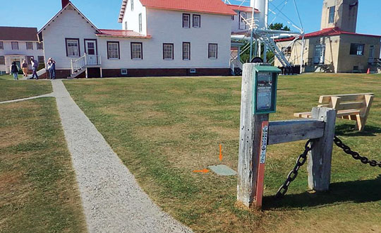
Figure 1: Utility access box installed over CORS reference mark Whitefish Pt A (NGS PID AA8050) at USCG lighthouse. (Photo: Jeff Olsen)
GNSS users who appreciate that physical monuments can provide verification of GNSS observations can do four things to preserve those monuments and make them more accessible. References below are to U.S. national agencies, but most countries have equivalent agencies.
Install a valve box over each buried control point recovered or set, whether the point is for boundary or geodetic surveying. Include National Geodetic Survey (NGS) deep-rod marks that have a buried logo cap.
Advocate with the Secretary of the Interior and United States Geological Survey (USGS) director that USGS scan its paper geodetic data sheets and post the scanned pdf files online.
Adopt the geodetic marks in your area. Visit them. Keep them free of brush or other blockages. Maintain descriptions and photos up to date by submitting recovery notes to NGS as needed. Participate in the NGS GPS on Benchmarks program.
Consider recovering all the marks in an NGS level line. Alternatively, all the USGS marks in a 15’ quadrangle, the geographic unit USGS uses to publish its geodetic data.
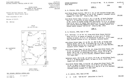
Figure 2: Example of USGS vertical data published by 15’ quadrangle.
Regarding the first of these actions, a valve box is a utility standard. It identifies to non-surveyors that there is something under the box to which one should pay attention, thus increasing the mark’s chances of survival.
The box lid is generally obvious, eliminating or at least reducing the search time for surveyors, who only need to walk up to the box.
It replaces the soil that previously covered the mark, reducing excavation time. A surveyor only needs to open the lid and brush off the mark. Rectangular and round boxes in several sizes are available to accommodate different-sized monuments. While the time and materials to install a box may be an overhead cost to your company, it is well worth the investment.
Regarding the second of these actions, the positions and heights published for most USGS control marks are based on superseded datums. However, that old data can be useful for evaluating trends. The marks are usually stable and can be reused in new projects.
While NGS has observed some of these marks and published datasheets for them, they are by far the minority of all the USGS marks in the country.
There are thousands of these sheets, 50 shelf-feet of them, organized by 15’ quad. Some sheets, mainly in the East, have been scanned and put online by various state agencies or utility companies. The USGS Rolla office has scanned most of the eastern states but has not posted the files online.
Generally, a request for USGS geodetic data turns into a request for paper sheets, such as those shown in Figure 2, to be scanned and emailed. Putting them online would preserve this record of what it took to survey and map our country, allowing the marks to be tied into new control surveys.
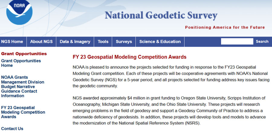
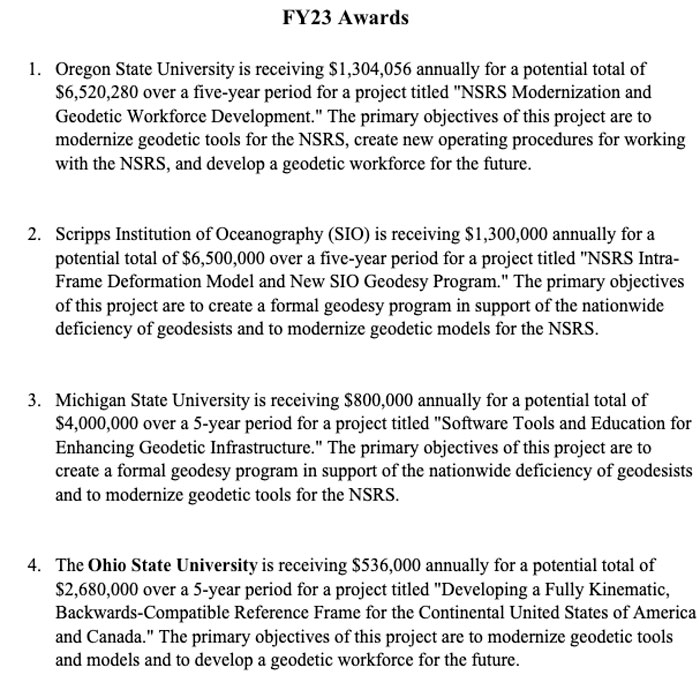
In my November 2023GPS World newsletter, I highlighted the announcement made by the National Geodetic Survey (NGS) of the recipients of the National Oceanic and Atmospheric Administration (NOAA) FY 2023 Geospatial Modeling Competition Awards. As stated in the newsletter, NGS awarded the grants for projects that will research emerging problems in the field of geodesy and develop tools and models to advance the modernization of the National Spatial Reference System (NSRS). A significant improvement in the new, modernized NSRS is the time-dependent component being incorporated in the computation of reference epoch coordinates (RECs). That said, developing models that accurately capture the time-dependent component is extremely important to providing reliable, consistent, and accurate RECs. This is not a simple problem to solve. Two of the grantees, Scripps Institution of Oceanography (SIO) and The Ohio State University (OSU) include developing models to address what NGS denotes as the Intra-Frame Deformation Model (IFDM).
This newsletter is going to highlight OSU’s geospatial award and my March newsletter will highlight the SIO proposal.
Summary of the OSU Geospatial Awards. (Image: NGS website)
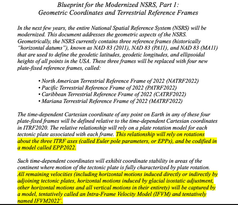
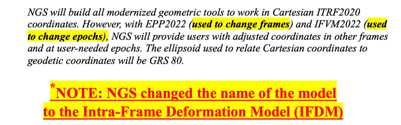
The time-dependent models for the new, modernized NSRS — that is, Euler pole parameters (EPP) and Intra-Frame Deformation Model (IFDM)] — are discussed in NOAA Technical Report NOS NGS 62, “Blueprint for the Modernized NSRS, Part 1: Geometric Coordinates and Terrestrial Reference Frames” and NOAA Technical Report NOS NGS 67, “Blueprint for the Modernized NSRS, Part 3: Working in the Modernized NSRS.” The EPP2022 and IFDM2022 models will make time-dependent geodetic control useable for most surveyors, engineers, and geospatial users.
So, what are EPP2022 and IFDM2022? What does it mean to users of the new, modernized NSRS? Basically, the EPP model changes the reference frame of the coordinates but not the epoch and the IFDM model changes the epoch of the coordinates but not the reference frame.
For the OSU grant proposal, I had the opportunity to talk with Dr. Demián Gómez, the lead principal investigator (PI) for the OSU grant. Demián has extensive experience in modeling time-dependent coordinates and is the lead author on several papers published in the Journal of Geodesy that address this topic.
Articles by Gómez in the Journal of Geodesy
Gómez, D., Piñón, D.A., Smalley, R. et al (2015) Reference frame access under the effects of great earthquakes: a least squares collocation approach for non-secular post-seismic evolution. J Geod. https://doi. org/10. 1007/s00190-015-0871-8
Gómez, D.D., Bevis, M. G. & Caccamise, D.J. Maximizing the consistency between regional and global reference frames utilizing inheritance of seasonal displacement parameters. J Geod 96, 9 (2022). https://doi. org/10. 1007/s00190-022-01594-0
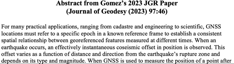
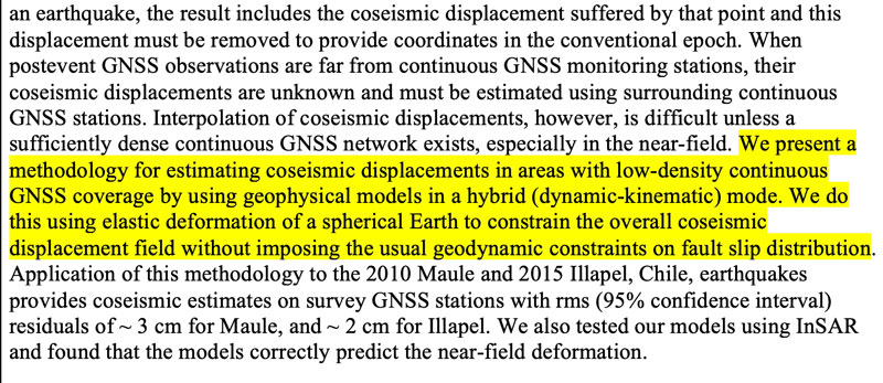
Gómez, D.D., Figueroa, M. A., Sobrero, F. S. et al. On the determination of coseismic deformation models to improve access to geodetic reference frame conventional epochs in low-density GNSS networks. J Geod 97, 46 (2023). https://doi. org/10. 1007/s00190-023-01734-0
In his latest paper, titled “On the determination of coseismic deformation models to improve access to geodetic reference frame conventional epochs in low-density GNSS networks,” the authors applied their methodology to two earthquakes in Chile: the 2010 Maule and 2015 Illapel earthquakes. The paper describes their methodology for estimating coseismic displacements in areas with low-density continuous GNSS coverage by using geophysical models in a hybrid (dynamic-kinematic) mode. Their methodology provided coseismic estimates on survey GNSS stations with rms (95% confidence interval) residuals of ~ 3 cm for Maule, and ~ 2 cm for Illapel. They also tested their models using InSAR and found that the models correctly predicted the near-field deformation. The authors believe that their methodology to obtain coseismic surface displacement models, based on a spherical layered Earth, for GNSS trajectory prediction models (TPMs) using sparse GNSS data represents a major improvement relative to coseismic models incorporated in TPMs, such as NGS’s Horizontal Time-Dependent Positioning model (HTDP) and Transformations in Four Dimensions (TRANS4D). This is important to users of the new, modernized NSRS because the accuracy of the IFDM2022 model is important to providing accurate RECs in the new, modernized NSRS.
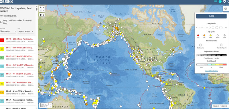
Most individuals in the United States associate earthquakes with California, but earthquakes occur every day in NGS’s area of responsibility. The USGS has a website that lists the location and magnitude of earthquakes.
Plot of earthquakes — 12/21/2023 to 01/20/2024. (Image: USGS website)
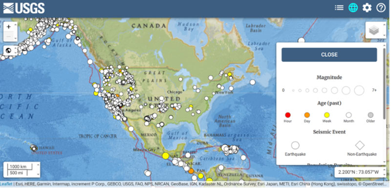
The box below highlights the earthquakes in the conterminous United States during a 30-day period. Most of these earthquakes have small magnitudes. The question is, what effects do these earthquakes have on nearby published marks in the NSRS?
Plot of earthquakes in CONUS — 12/21/2023 to 01/20/2024. (Image: USGS website)
The website provides information on both earthquake and non-earthquake events.
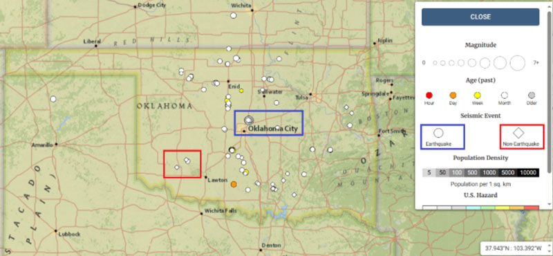
Plot of earthquakes in Oklahoma — 12/21/2023 to 01/20/2024. (Image: USGS website)
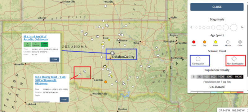
I was wondering what it meant by non-earthquake events, so I clicked on some of the icons. As indicated on the plot, a quarry blast registered on the USGS system. Again, the question is, do these earthquakes and non-earthquake events affect the coordinates of marks in the ground?
Plot of non-earthquakes in Oklahoma. (Image: USGS website)
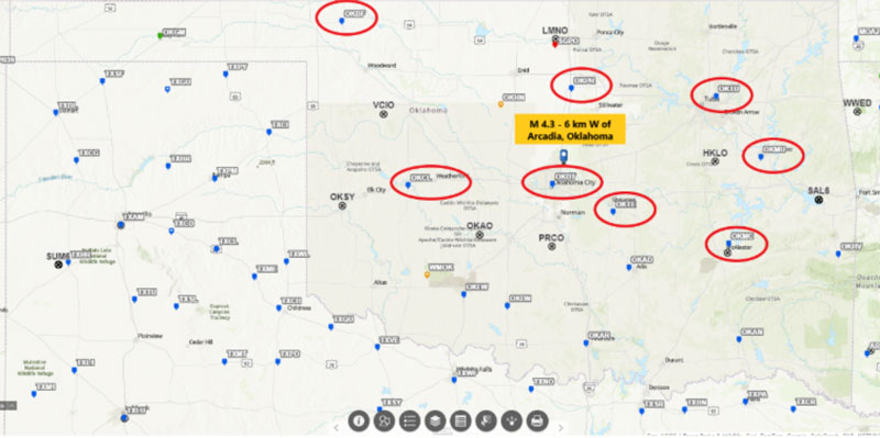
Something to note in the plots of Oklahoma is the large number of earthquakes around Oklahoma City during a 30-day period.
Plot of earthquakes north of Oklahoma City. (Image: USGS website)
Notice that there are several CORSs that surround the location of the earthquakes but only one CORS is close to the area. The box below shows a plot of CORS surrounding the area of earthquakes.
Demián’s latest paper describes their methodology for estimating coseismic displacements in areas with low-density continuous GNSS coverage by using geophysical models in a hybrid (dynamic-kinematic) mode. Since many earthquakes occur throughout the United States, it will be interesting to see how well this approach will work in the development of an Intra-Frame Deformation Model.
Earthquake M 4. 3 – 6 km W of Arcadia, Oklahoma. (Image: NGS website)
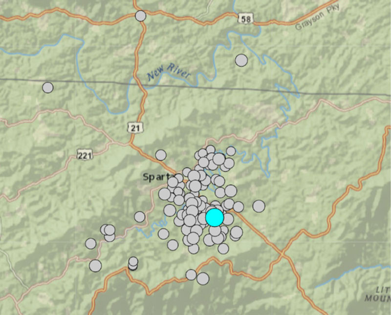
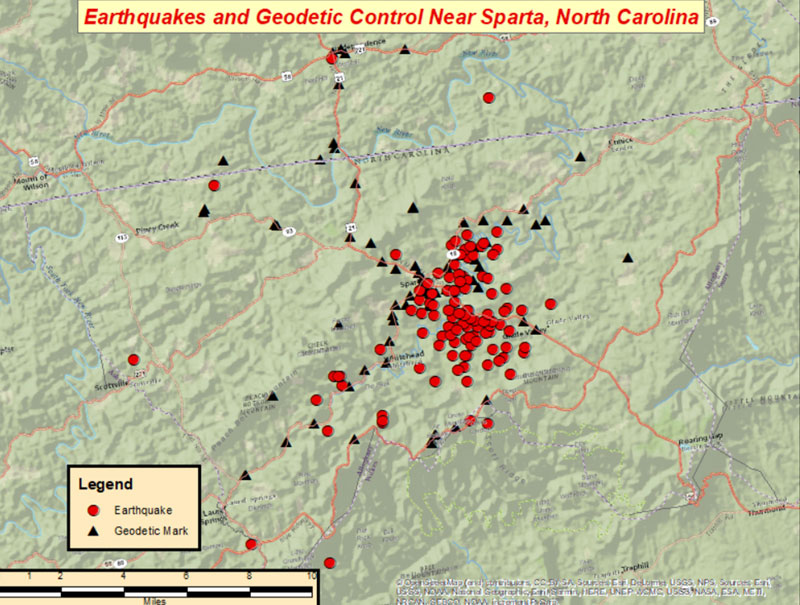
As previously stated, outside of California, most of these earthquakes have small magnitudes. That said, on August 9, 2020, a magnitude 5.1 earthquake occurred in Sparta, North Carolina. There were reports of damage to roads, water mains, and structures, but what were the effects on nearby published marks in the NSRS?
Widespread damage occurred in Sparta, which had already been debilitated by the COVID-19 pandemic in North Carolina. [23] Damages include collapsed ceilings, chimneys, and masonry; damaged water mains; cracked and deformed roads; uprooted headstones; and displaced appliances and items. [24][23][25] Wes Brinegar, the town’s mayor, issued a state of emergency to apply for FEMA and state financial aid. [25][23] Damage was worse than initially thought, with at least 525 structures being damaged, and 60 with major damage, meaning at least 40% of the structure was a total loss. Nineteen people lost their homes, 25 were declared uninhabitable, and scammers took advantage of the damage, charging people up to $500 USD for repairs, but never showing up.[26]
Governor of North Carolina, Roy Cooper, toured the damage in Sparta, releasing a statement later, stating “We’ve dealt with a hurricane, a violent tornado, and now an earthquake all in the middle of a pandemic: North Carolinians are resilient.”[27]
The box below shows the locations of earthquakes that occurred near Sparta, North Carolina. The plot indicates that there was not just one earthquake in the area, but many that may have affected the coordinates of monuments in the region.
Plot of earthquakes near Sparta, North Carolina. (Image: USGS website)
The image below shows the locations of earthquakes and NGS published geodetic marks in the Sparta region.
Image: Dave Zilkoski
Again, the real issue that needs to be addressed is what effect do these earthquakes and other geophysical activities such as subsidence have on the coordinates of geodetic marks in the region?
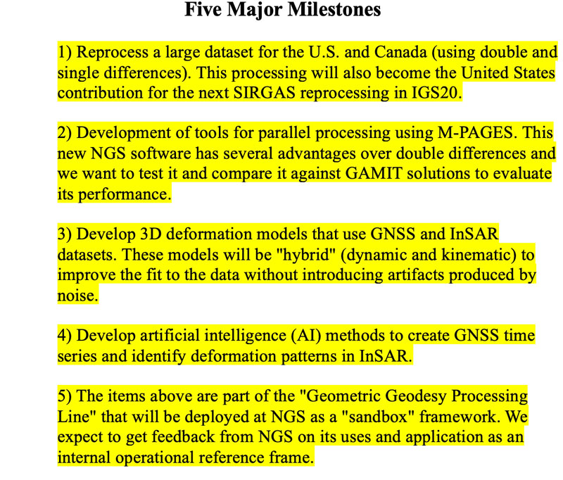
OSU’s grant proposal includes merging GNSS and InSAR using deep learning to better estimate the Intra-Frame Deformation Model. Obviously, developing time-dependent models for the new, modernized NSRS is very complex and technical. I contacted Demián and asked him for a list of his major milestones associated with his project.
Based on Demián’s major milestones, I had a few follow-up questions.
1) Reprocess a large dataset for the U.S. and Canada using double and single differences. This processing will also become the United States’ contribution for the next SIRGAS reprocessing in IGS20.
I asked Demián if he had an estimate of the amount of data he was talking about?
He told me that he did not have an exact number yet because they are still adding data. He said that, at this time, they have 878 stations in the US and Canada which amounts to 4,648,269 station days (i.e., 4. 6M RINEX files, just in the US and Canada). This is the latest number he retrieved from his database but this number increases every day (January 16, 2024).
2) Development of tools for parallel processing using M-PAGES. This new NGS software has several advantages over double differences and we want to test it and compare it against GAMIT solutions to evaluate its performance.
Demián stated that M-PAGES has several advantages so I asked him to explain what he meant.
He told me that one advantage is that it can process all constellations at once using single differences which allows processing of more stations simultaneously. Another advantage is because single differences produce “lighter” systems of equations (compared to double differences), they can process more stations simultaneously.
3) Develop 3D deformation models that use GNSS and InSAR datasets. These models will be “hybrid” (dynamic and kinematic) to improve the fit to the data without introducing artifacts produced by noise.
[Note: this approach is described in the paper titled “On the determination of coseismic deformation models to improve access to geodetic reference frame conventional epochs in low-density GNSS networks,” J Geod 97, 46 (2023).]
Demián said“they are in the process of collecting all the GNSS data that they can to process and then they will identify which gaps can be filled with InSAR data.”
I wanted to better understand what Demián meant by “hybrid” model. So, I asked him about his “hybrid” approach and he provided the following explanation:
When we say “kinematic” we refer to a model that does not consider the underlying mechanism to explain the observed effect. A good example are the trajectory models of GNSS stations that describe their motions as a sum of mathematical functions (there are no physics in them). A dynamic model does use the underlying physics to explain the observations. A “hybrid” model is in the middle: it uses a dynamic model but allows some unrealistic model parameters to improve the data fit.
I mentioned to Demián that users would be very interested in the spatiotemporal uncertainties of the intra-frame deformation model. I asked him if, at this time, he had any idea of the size or range of uncertainties.
Demián said “that it will be variable and very dependent on the density of the input data. He said that they are aiming for cm-level uncertainties. Our experience in Argentina tells us that a 5 mm uncertainty level can be achieved on stable regions while about 2 to 3 cm is expected on high deformation areas. We will have to wait and see to understand the model’s performance. ”
I told Demián that the Houston-Galveston, Texas region of the United States is an area of subsidence that would benefit with an accurate Intra-Frame Deformation Model. The Harris-Galveston Subsidence District has a variety of GNSS CORS and PAMS that are not part of NGS’s CORS. My April 2022 GPS World Newsletter, which included the HGSD CORS and PAMS, described the effects of vertical movement on NGS’s modernized 2022 NSRS. I also asked if he was willing to use this data
He had a very simple answer: “Absolutely!” He said “The more data we incorporate, the better the models will describe reality. Part of the project is related to providing a processing line that can handle large amounts of data. The issue with some data is metadata. Metadata and how we collect it is what really prevents us from reaching that “final mm” uncertainty level we are all looking for. We should be pushing very hard on metadata standardization. In my opinion, the biggest problem is twofold: 1) incorrect antenna identification in RINEX files (due to improper data curation) and 2) lack of a unified/globally accessible database of metadata that is adequately cured.”
4) Develop AI methods to create GNSS time series and identify deformation patterns in InSAR.
Part of the OSU project is to use ML to improve the development of the IFDM.
Excerpt from OSU Proposal on trajectory modeling
Trajectory modeling
For each station, we will obtain KTM parameters, including their uncertainties, for
stations velocities (and acceleration if needed), mechanical and/or geophysical jumps (earthquakes), logarithmic transients after earthquakes (following recommendations from Sobrero et al., 2020), and seasonal coordinate variations. Other parameters for stations affected by volcanic activity, episodic subsidence, etc will also be added when needed. We routinely generate these KTMs for thousands of GNSS stations (for the definition of our in-house geodetic RF) using software developed within the Division of Geodetic Science at OSU. Earthquake detection is performed automatically following formulations also developed by the project’s PIs.
Trajectory modeling enhancement using machine learning
We will enhance the capabilities of the KTMs by including a physics-based machine
learning (ML) component to the model that automatically detects, e. g., discontinuities in the time series. Detecting and mitigating the effects of mechanical jumps (those generated by unreported equipment changes and other effects) will increase the overall reliability of the GGPL. ML is well suited for this task and indeed ML algorithms like Random Forests have been explored in a recent work (e. g., Crocetti et al., 2021). We will test a similar approach, as well as more sophisticated convolutional neural networks to automatically detect discontinuities in coordinate trajectories. These ML algorithms will be trained on OSU’s database of trajectory models (~4000 stations). Using this ML algorithm we will also automatically detect other ‘harmful’ residuals in the time series. For example, large residuals can appear right after an earthquake if the postseismic transient does not have the appropriate relaxation time, or if two transients are needed to model the event.
I find AI and ML fascinating. Basically, machine learning is a field of study in artificial intelligence.
[As a side note: According to Wikipedia, Alan Turing, a mathematician, was the first person to conduct substantial research in the field that he called machine intelligence. Mr. Turing was considered the father of modern computer science. He was famous for his work in decoding the encryption of German Enigma machines during the second world war, and documenting a procedure, known as the Turing Test, that formed the basis for artificial intelligence. Turing was not directly involved with the successful breaking of these more complex codes, but his ideas proved of the greatest importance in this work.]
5) The items above are part of the “Geometric Geodesy Processing Line” that will be deployed at NGS as a “sandbox” framework. We expect to get feedback from NGS on its uses and application as an internal operational reference frame.
The fifth milestone includes developing what Demián calls a “Geometric Geodesy Processing Line (GGPL).” GGPL has three phases, but I am very interested in the first phase. The first phase will begin by analyzing the different components of the GGPL, including the interactions with various geospatial stakeholders, both within and outside of the United States. The plan includes developing a workflow that involves data curation, processing, and analysis to create an operational, fully kinematic reference frame (KRF) for CONUS and Canada. The KRF, once implemented, would at first constitute an experimental or ‘sandbox’ frame executed jointly with NGS’s Geosciences Research Division.
I asked Demián what plans he has for involving users. Especially, how is he going to include surveyors, engineers, photogrammetrists, and spatial data managers?
“My goal is to bring some of the lessons learned in Argentina when we implemented the kinematic reference frame in 2019,” Demián said. Back then, we had discussions with small groups of people in industry to know what their needs were. For example, surveyors will probably need to deal with epoch transformations in a different way than engineers or spatial data managers. The GGPL should facilitate the products that will help these stakeholders. In my experience, the issue is how the data (or model) is accessed so I do not foresee any major issues with users.”
He said that he is open to any suggestions others might have about this.
In phase two, OSU will augment the KRF with locally ‘dynamic’ densifications, which allow
the reference frame to be ‘interpolated’ to locations between the reference stations. Using advanced techniques, such as deep learning, complementary datasets, such as GNSS and InSAR, will be combined and assimilated leading to a kinematic/dynamic reference frame. During phase two, NGS would be assessing the utility and performance of the sandbox GGPL, while OSU works on its dynamic extensions.
In a third phase, the GGPL and the associated KRF and models would undergo any necessary modifications and adaptations, all guided by NGS. By the end of the proposed project, NGS will have a sandbox frame that can implement any new International Terrestrial Reference Frame (ITRF) in a manner that is completely transparent to NSRS users, including all associated models to operate continuously and without interruption.
This newsletter highlighted NGS’s grant to OSU for developing a fully kinematic reference frame for the Continental United States of America and Canada. The primary objectives of this project are to modernize geodetic tools and models and to develop a geodetic workforce for the future. The OSU project will include interactions with various geospatial stakeholders, both within and outside of the United States. In my opinion, it is very important to engage the geospatial user community when developing these new tools so the tools will be useful during the implementation of the new NSRS. A significant improvement in the new, modernized NSRS is the time-dependent component being incorporated in the computation of reference epoch coordinates (RECs). That said, developing models that accurately capture the time-dependent component is extremely important to providing reliable, consistent, and accurate RECs. The goal of the OSU project is to provide an accurate Intra-Frame Deformation Model which will provide reliable, consistent, and accurate reference epoch coordinates (RECs). Throughout the project, OSU would train M.S. and Ph.D. students, and postdocs, providing a source of trained new employees for governmental agencies as well as private industry. Future newsletters will address other NGS recipients of the NOAA FY 23 Geospatial Modeling Competition Awards.
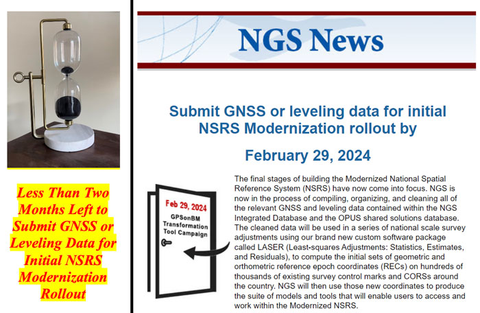
The National Geodetic Survey (NGS) has announced that users have until February 29, 2024, to submit data for the initial National Spatial Reference System (NSRS) modernization rollout. This means time is running out to submit GNSS or leveling data for initial NSRS Modernization. It is anticipated that NGS will release the new, modernized NSRS in 2025, once new data is incorporated into the database. The following newsletter will provide some advice on strategically selecting marks to improve the local accuracy of the NAVD 88-to-NAPGD 2022 transformation tool.
Image: NGS website
As the announcement stated, NGS is in the process of compiling, organizing, and cleaning all the relevant GNSS and leveling data contained within the NGS Integrated Database and the OPUS shared solutions database for preparation of the new, modernized NSRS. The data will be used in national scale survey adjustments using NGS’ new software package called LASER (Least-squares Adjustments: Statistics, Estimates, and Residuals). The adjustments will compute the initial sets of geometric and orthometric reference epoch coordinates (RECs) on many existing survey control marks and CORS around the country. The definitions of RECs and survey epoch coordinates (SECs) are spelled out in NOAA Technical Report NOS NGS 67, NGS’s Blueprint Part 3. My April 2021GPS World newsletter highlighted the Blueprint Part 3 document, and my August 2022GPS World newsletter provided details on RECs and SECs. Using the results of the adjustments, NGS will produce a suite of models and tools that will enable users to access and work within the Modernized NSRS.
During the last several years, NGS’ GPS on Benchmarks program has been encouraging stakeholders and partners around the country to submit GNSS data to NGS on marks that they use. This will ensure that these marks will have updated RECs when the new system is implemented. Also, just as important, marks that also have North American Vertical Datum of 1988 (NAVD 88) heights will be used to improve the local accuracy of the NAVD 88-to-NAPGD 2022 transformation tool.
NGS’ plans include accepting user data, but after February 29, 2024, they will not include additional GNSS and leveling data for the initial REC national adjustment and for use in building the transformation tools. In 2018, I wrote a series of GPS World newsletters that highlighted NGS’ GPS on BM program (February 2018, April 2018, June 2018, and August 2018). At that time, the GPS on BM program was very useful in the development and implementation of the hybrid geoid model GEOID18. This newsletter will provide an update on the GPS on BM Transformation Program and provide some advice on strategically selecting marks to improve the local accuracy of the NAVD 88-to-NAPGD 2022 transformation tool.
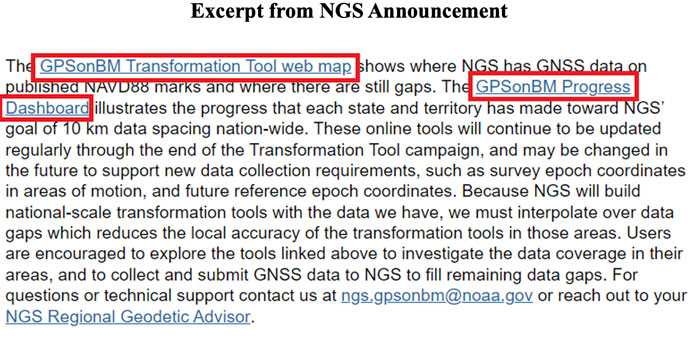
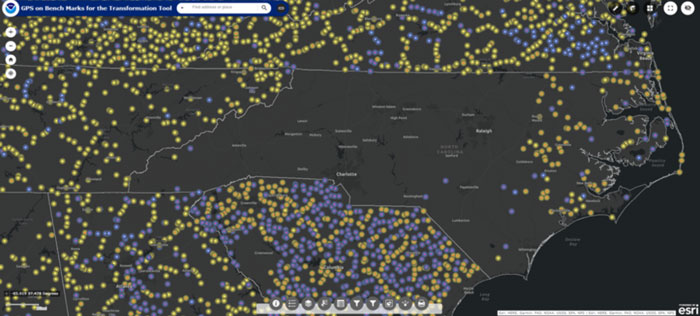
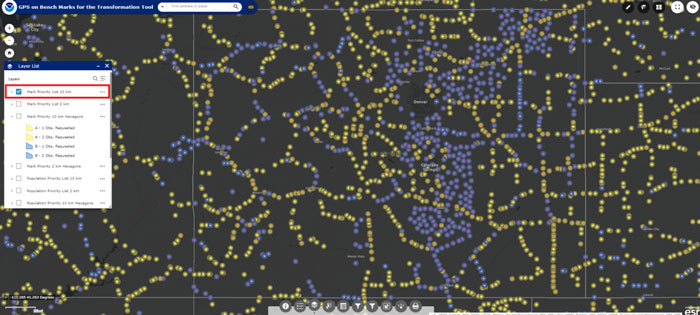
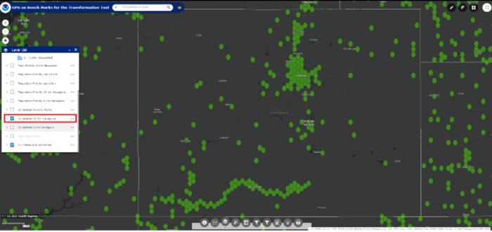
When users click the link GPSonBM Transformation Tool Web Map, they are connected to a web map depicting a prioritized list of marks where new GNSS observations would be most helpful to the development of the transformation model between the current vertical datum (e.g., NAVD 88) and the modernized NSRS.
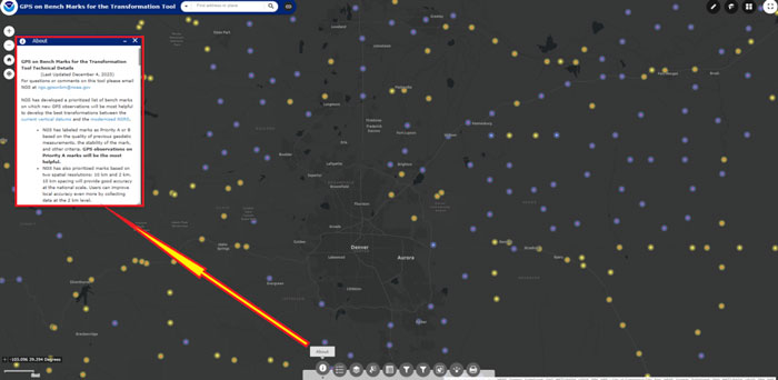
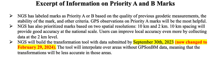
NGS’ prioritized list of benchmarks are labeled as Priority A or B. Clicking on the “About” button on the webpage provides information about the priority marks. See the boxes titled “GPSonBM Transformation Tool Web Map” and “Excerpt of Information on Priority A and B Marks.”
GPS on BM Transformation Tool Web Map. (Image: NGS website)
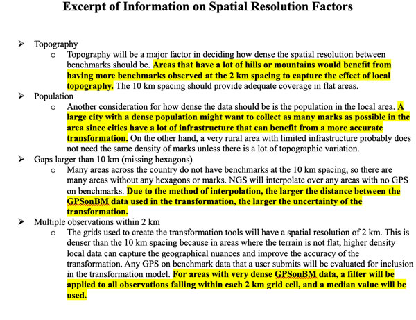
To assist users in their selection of marks, NGS developed criteria based on spatial resolution factors. See the box titled “Excerpt of Information on Spatial Resolution Factors.” As previously stated, time is running out. In my opinion, users should prioritize their GPS on BM plans based on the NGS’ criteria. I have highlighted what is important for users to consider when selecting marks.
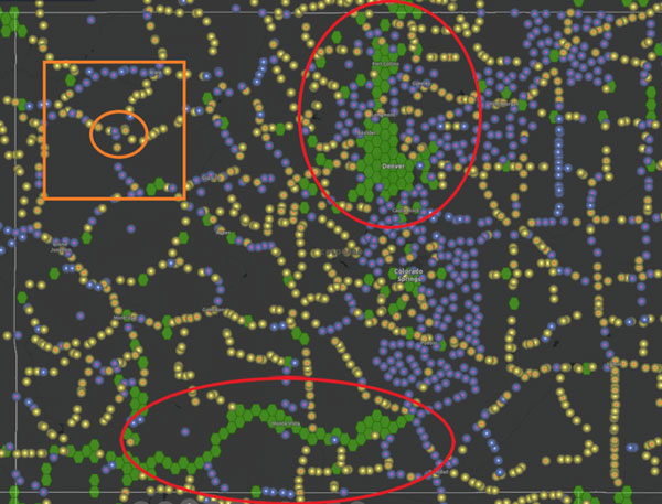
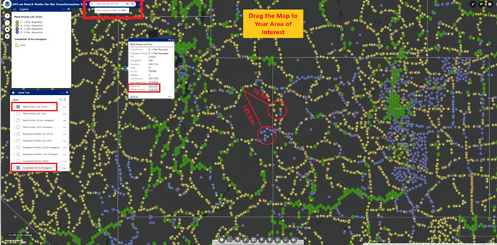
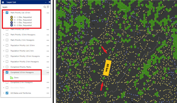
Many areas across the country do not have benchmarks at the 10 km spacing, so there are some areas without any hexagons or marks. As stated in the spatial resolution factors, NGS will interpolate over any areas with no GPS on benchmarks. In areas that have gaps larger than 10 km, that is, that are missing hexagons, I would recommend occupying several marks in each hexagon surrounding the gap to ensure that marks with valid NAVD 88 heights are part of the transformation tool. The web tool defaults to the Denver, Colorado, region when you access it but users can drag the map to an area of their interest or select a location.
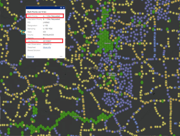
Locating marks using the GPSonBM transformation tool web map. (Image: NGS Website)
Acquiring data in mountainous regions and areas that have large distances between completed hexagons is probably the most important for users to focus on. The box titled “Locating Marks Using the GPS on BM Transformation Tool Web Map” provide marks that need to be observed. As an example, I have highlighted two areas that have large distances between benchmarks and completed hexagons. In this case, it would be important to occupy a couple of marks in the highlighted locations. Clicking on a mark provides a box with the following information: Mark Priority, Population Priority, PID, Designation, Stamping, State, County, Stability code, Last Date of Recovery, Last Date of Observation, Link to NGS Datasheet, and a Link to a Shared Solution (if one exists).
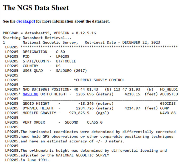
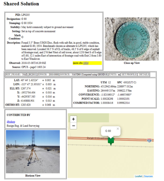
Clicking the link titled “More Info” next to Datasheet brings up the NGS datasheet for the mark, and clicking the link titled “More Info” next to Shared Solution” brings up the Shared Solution information (see the boxes titled “Mark Priority Information for Mark G 80,” “Excerpt from NGS Datasheet for Mark G 80,” and “Shared Solution for Mark G 80.”). I would recommend that State surveying organizations (and surveyors) perform this type of analysis and strategically occupy marks that fill in important gaps. There is less than two months remaining to submit data to NGS that will support the transformation tool.
Excerpt from NGS datasheet for Mark G 80. (Image: NGS website)Shared solution for Mark G 80. (Image: NGS website)
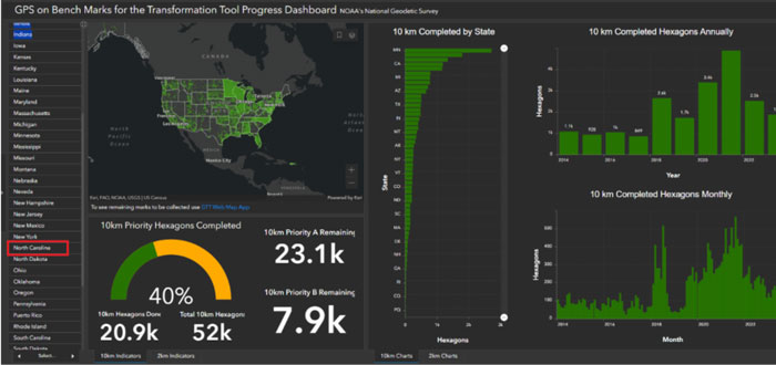
The GPSonBM Progress Dashboard illustrates the progress that each state and territory has made toward NGS’ goal of 10 km (and 2 km) data spacing nationwide.
GPSonBM Program Dashboard. (Image: NGS website)
Users can see the GPS on Benchmark information for a particular state by clicking on the name of the state on the left side of the website.
Selection of North Carolina. (Image: NGS website)
I highlighted North Carolina because I live in that state. The map informs the users of how many 10 km priority A (89) and B (32) marks are remaining to be occupied, and the percentage completed (92%). Clicking on the link “To see remaining marks to be collected use GTT Web Map App,” located under the map, depicts the remaining marks to be collected. As you can see from the plot, North Carolina has several marks in the eastern portion of the state that still need to be occupied with GNSS.
Status of GPS on benchmarks in North Carolina. (Image: NGS website)
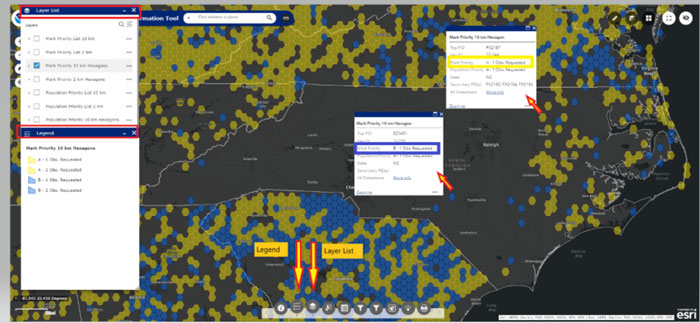
A nice feature of the map is the legend and layer list buttons. Also, information about the mark appears if you click on a mark.
Example of legend and layer list. (Image: NGS website)
The image below provides a list of layers that can be selected using the webtool.
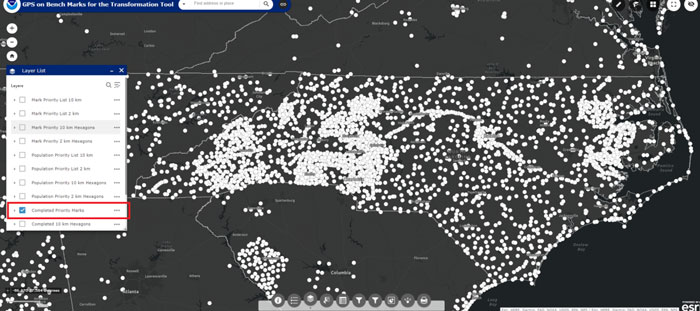
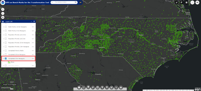
The following image depicts marks that have been completed. As you see from the plot, North Carolina has been very active in the GPS on Benchmark program.
Completed marks in North Carolina. (Image: NGS website)
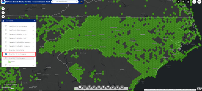
Users can also click on the button to see which 10 km (and 2 km) hexagons have been completed (see the boxes titled “Completed 10 km Hexagons in North Carolina” and “Completed 2 km Hexagons in North Carolina”).
Completed 10km Hexagons in North Carolina. (Image: NGS website)Completed 2km Hexagons in North Carolina. (mage: NGS website)
The North Carolina Geodetic Survey, under the leadership of Gary Thomson, along with NC surveyors has been involved with the GPSonBM program from its inception.
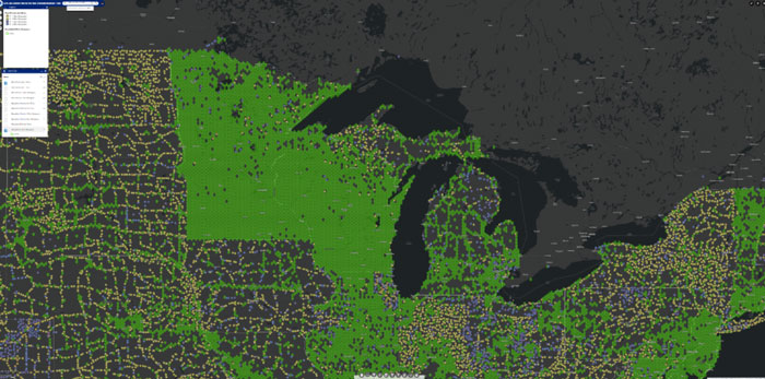
As previously stated, the website provides the list of priority benchmarks and the status of GPS on Benchmark for each state. There are other states that have been very active in the GPS on Benchmark program such as Minnesota and Wisconsin.
Completed 10 km Hexagons in Great Lakes Region. (Image: NGS website)
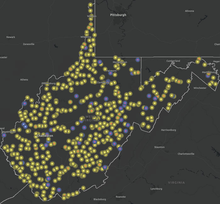
The following images provide the GPS on Benchmark information for West Virginia.
Status of GPS on benchmarks in West Virginia. (Image: NGS website)Completed marks in West Virginia. (NGS website)Completed 10 km hexagons in West Virginia. (Image: NGS)
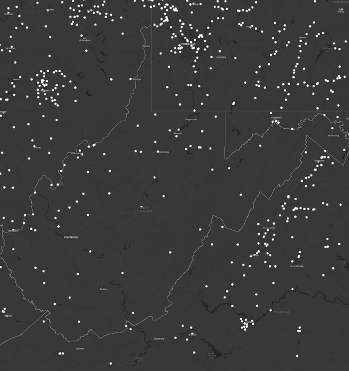
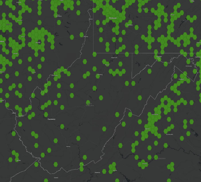
The following image provides a plot of an area in West Virigina that highlights a region with a large gap between completed 10 km hexagons. If a user was interested in supporting the development of the transformation model in West Virigina, occupying a mark with GNSS in this area would help improve the local accuracy of the NAVD 88-to-NAPGD 2022 transformation tool.
Overlay of completed and status of benchmarks in West Virginia. (Image: NGS website)
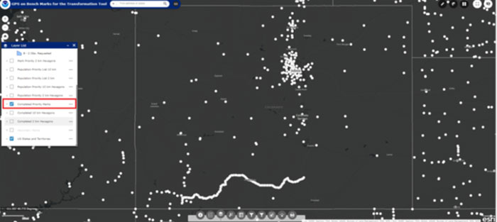
North Carolina and West Virginia are not large states compared to some western states. The boxes titled “Status of GPS on Benchmarks in Colorado,” “Completed Marks in Colorado,” “Completed 10 km Hexagons in Colorado,” and “Overlay of Completed and Status of Benchmarks in Colorado” provide the information for Colorado. Looking at the plots there appears to be many regions that could use GPS on Benchmark occupations.
Status of GPS on benchmarks in Colorado. (Image: NGS website)Completed marks in Colorado. (Image: NGS)Completed 10 km hexagons in Colorado. (Image: NGS website)
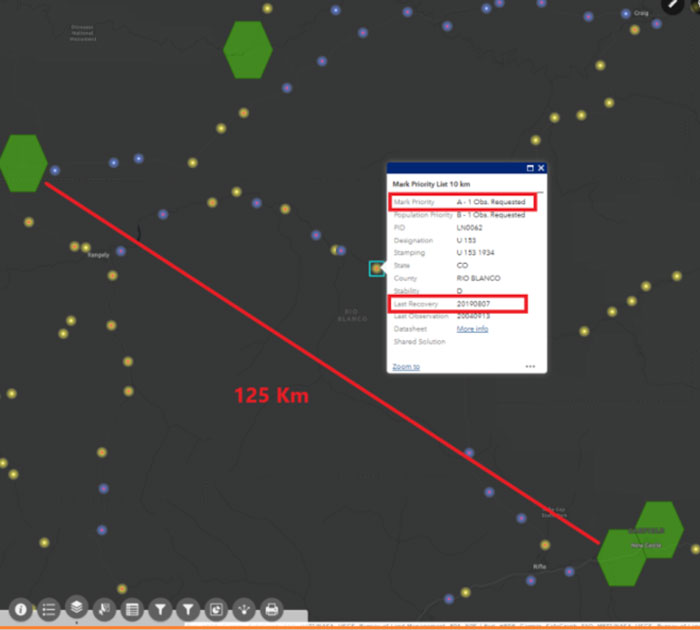
Looking at the plot in the image below, there appear to be many marks that were occupied in populated areas such as Denver, Fort Collins, and Colorado Springs. The marks along the southern border were part of NGS’ 2017 Geoid Slope Validation Survey (GSVS) Project. The area highlighted by the orange box is an area that is lacking GPS on Benchmark occupations. The distance between the nearest completed 10 km hexagon is 60 kilometers. In other words, the two completed hexagons are more than 120 km apart. As previously stated, NGS will interpolate over any areas with no GPS on benchmarks.
Overlay of completed and status of benchmarks in Colorado. (Image: NGS website)
Again, in areas that have gaps larger than 10 km with missing hexagons, I recommend occupying several marks in each hexagon surrounding the gap to ensure that marks with valid NAVD 88 heights are part of the transformation tool. To demonstrate this concept, I have selected an area in Colorado near benchmark U 153 (PID LN0062).
Benchmark U 153 in Colorado. (Image: NGS website)
The following image depicts the locations of the completed hexagons near benchmark U 153.
NGS has developed web tools to assist users in the selection of marks for the program. Two web tools that I find useful are the Leveling Project Page and the Passive Mark Page. The Leveling Project Page provides information on leveling line data. Users can find information about the marks involved with a certain leveling line. There are links to the Passive Mark Page and NGS datasheets on the Leveling Project Page. My October 2020GPS World newsletter described the Passive Mark Page web tool in more detail, and my June 2021GPS World newsletter demonstrated the use of the tools.
In this example, I selected U 153 because it was located between two completed 10 km hexagons that are 125 km apart. That said, looking at the information from the passive mark web tool, it appears that the published height of the benchmark is based on 1934 leveling data. That by itself is not a bad thing but the Orthometric Height Residual is very large (-23.1 cm). This implies that the difference between the GNSS-derived orthometric height using Geoid18 and the published NAVD 88 height disagreed by 23.1cm. This could be due to the movement of the mark and, in my opinion, is not a good candidate for the transformation tool.
As previously stated, NGS’ Leveling Project Page, provides information on the benchmarks and associated data involved in a leveling line. See the box titled “Excerpt from NGS Leveling Project Page for L2577.” Users can find information about all the marks involved with a certain leveling line.
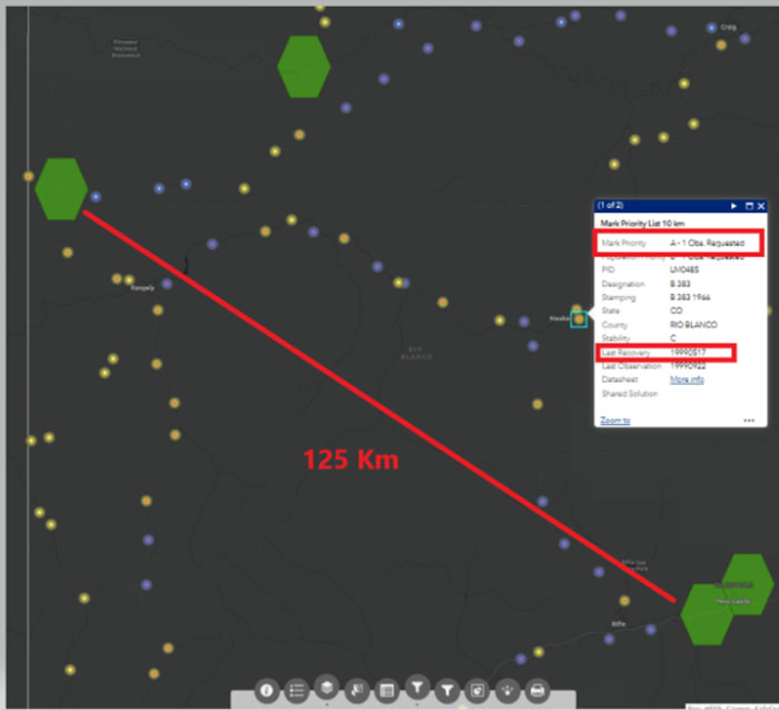
Excerpt from NGS Leveling Project page for L2577. (Image: NGS website)Distance between 10km hexagons near B 383 in Colorado. (Image: NGS website)
Again, I used the Passive Mark tool to find detailed information about the mark. See the box titled “Excerpt from NGS Passive Mark Tool for B 383.” This mark was last leveled in 1966 and the Orthometric Height Residual is small (1.2 cm). This implies that the difference between the GNSS-derived orthometric height using Geoid18 and the published NAVD 88 height disagreed by 1.2 cm.
This could be a good candidate for the GPS on BM program and the transformation tool.
Excerpt from NGS passive mark tool for B 383. (Image: NGS)
For completeness, I looked at another mark in the same area.
Distance Between 10km hexagons near B 154 in Colorado. (Image: NGS website)
I highlighted this mark because it was last leveled on the same 1934 leveling line as mark U 153. Unlike U 153, looking at the information provided by the Passive Mark tool for B 154 indicates that the GNSS-derived orthometric height agrees with the published leveling-derived orthometric height. The orthometric height residual is only -2.1 cm. This would be another good candidate to fill the area between the two completed hexagons.
This newsletter provided some advice on strategically selecting marks to improve the local accuracy of the NAVD 88-to-NAPGD 2022 transformation tool. Again, I would recommend that state surveying organizations and surveyors perform the analysis described above and strategically occupy marks that fill in important gaps. There is less than two months remaining to submit data to NGS that will support the transformation tool.
NGS has developed web tools such as Passive Mark Page and Leveling Project Page to assist users in identifying marks for inclusion in the development of the transformation model between the current vertical datums (e.g., NAVD 88) and the modernized NSRS.
When Boston Light — an 89 ft-high, white lighthouse on Little Brewster Island in Boston’s outer harbor — opened in September 1716, it was the first one in the Thirteen Colonies. Sally Snowman, who has been its keeper for most of the past two decades, is the last official lighthouse keeper in the United States. Contemplating the horrible trips across the Atlantic on merchants’ galleons, when many gale-tossed passengers despaired of ever setting foot on land again, she recently commented: “Imagine what they felt when they spotted the light.” See Dorothy Wickenden’s article “Last Watch” in the November 6, issue of my favorite magazine, The New Yorker. Of the roughly 850 lighthouses currently in the United States, Wickenden reported, only about half serve as active aids to navigation and the U.S. Coast Guard has automated all of them. “The rest,” Wickenden wrote, “have been made obsolete by GPS.” Yet, she pointed out, even hardheaded ship captains and pilots say that “lighthouses still have a place.”
When Snowman retires at the end of this month, it will mark the end of an era that lasted more than three centuries. This month also marks the 50th anniversary of the approval of Navstar GPS (as it was originally called) by the Defense Systems Acquisition Review Council (DSARC) of the U.S. Department of Defense. Three months earlier, at the meeting now remembered as Lonely Halls (see my editorial in the September issue), Brad Parkinson and his team had made the key decisions about the system’s architecture, including the number of satellites, their orbits, and what kinds of signals to use.
In this month’s issue, we revisit how, after initial opposition, the U.S. armed forces adopted GPS; how the civilian/commercial GPS (now GNSS) industry was born; and how surveyors reacted to this disruptive new technology.
To answer the first question, I asked Gaylord Green, who was on Parkinson’s team and later led the GPS Joint Program Office, to write his recollections on the subject. I also interviewed Marty Faga, whose long and distinguished career included four years as both Director, National Reconnaissance Office and Assistant Secretary for Space, U.S. Air Force. Faga passed away on October 19. To answer the second question, I turned to Charlie Trimble, who in 1978 co-founded the company named after him and was its CEO until 1998. To answer the third question, I chose Dave Zilkoski, who earned a master’s degree in geodetic science in 1979, the year after the first GPS satellite was deployed, while working for the National Geodetic Survey, of which he was later the director for about three years. Many readers of this magazine also know Zilkoski as the regular contributor to one of our four digital newsletters, Survey Scene.
On Oct. 26, 2023, I participated in an American Society for Photogrammetry and Remote Sensing (ASPRS) Pacific Southwest Region Fall Technical webinar. The webinar provided an overview of the ASPRS Positional Accuracy Standards for Digital Geospatial Data (Edition 2, Version 1.0 – August 2023). The document can be downloaded here.
ASPRS Webinar Announcement. (Image: ASPRS)
I also participated — virtually — in the Nov. 2, 2023, California Spatial Reference Center (CSRC) Coordinating Council fall meeting where Dr. Riadh Munjy, California State University, Fresno, discussed the revisions to the ASPRS Positional Accuracy Standards for Geospatial Data.
The most significant changes introduced in this second edition of the standards include:
Elimination of references to the 95% confidence level as an accuracy measure.
Relaxation of the accuracy requirement for ground control and checkpoints.
Consideration of survey checkpoint accuracy when computing final product accuracy.
Removal of the pass/fail requirement for Vegetated Vertical Accuracy (VVA) for lidar data.
Increase the minimum number of checkpoints required for product accuracy assessment from 20 to 30.
Limiting the maximum number of checkpoints for large projects to 120.
Introduction of a new term: three-dimensional positional accuracy.
Addition of Best Practices and Guidelines Addenda for:
General Best Practices and Guidelines
Field Surveying of Ground Control and Checkpoints
Mapping with Photogrammetry
Mapping with Lidar
Mapping with UAS
As outlined above, Edition 2 contains Best Practices and Guidelines for (1) General Best Practices and Guidelines and (2) Field Surveying of Ground Control and Checkpoints. The three addenda listed in the table of contents: Mapping with Photogrammetry, Mapping with Lidar, and Mapping with UAS will be available for public comment later, and will be added to Edition 2, Version 2.0.
Dr. Abdullah informed me that these addenda are on track to be put out for public comments during December 2023, therefore he believes they will probably be published in January or February 2024. The box titled “Summary of Significant Changes in Edition 2” provides the changes with the reason and justification for each change. The document can be downloaded from ASPRS here.
One of the changes is to relax the accuracy requirement for ground control and checkpoints. At first glance, this seems like the wrong thing to do. However, after understanding the justification, the requirement for ground truth still needs to be at least twice as accurate as the product.
Both Dr. Abdullah and Dr. Munjy’s emphasized in their presentations that the current accuracy requirements for ground controls in photogrammetric work of four-times better than the produced products, and the checkpoint accuracy requirement is three-times better than the assessed product. This makes it difficult, if it is not impossible, to use RTK-based techniques for this type of surveying. This by itself is not the reason for the change. During Dr. Abdullah’s presentation, he provided the following reasons for the change:
“Experience taught us that the requirements of four-times and three-times adopted in edition 1 of the standards are excessive and too restrictive, partly due to the reason outlined in (b) below.
Today’s sensors, software, and processing methodology are more accurate and the room for errors in the product is diminishing, therefore we do not need a safety factor of 3 or 4 to obtain accurate products.
Increasing demand for higher accuracy geospatial products.”
The new standards now factor in the accuracy of the survey checkpoints when determining the accuracy of the product. During Dr. Abdullah’s presentation, he provided the following reason for the change, “As we are producing more accurate products, errors in surveying techniques of the checkpoints used to assess product accuracy, although small, can no longer be neglected and it should be represented in computing the product accuracy.” He also highlighted that, “As product accuracy increases, the impact of error in checkpoints on the computed product accuracy increases.” The document provides equations used to compute the values. See below.
A very significant change, in my opinion, is the removal of the standards for Vegetated Vertical Accuracy (VVA) for lidar data. See below.
VVA not used as a criterion for acceptance. (Image: ASPRS)
I am not sure I agree with the reasoning, but I understand why it was done. GNSS-based surveys do not perform well in vegetated areas, and this is the technology used to validate the non-vegetated vertical accuracies (NVA). That said, there are non-GNSS technologies — sometimes denoted as traditional surveying methods — that could be used to validate VVA, so this seems like an elimination of a requirement based on the limitation of a particular technology.
Traditional surveying methods that use geodetic levels, theodolites, and total stations to measure distances, angles, and heights are still used by surveyors to perform certain projects. Since there are other surveying methods that could be used for evaluating the VVA, it does not seem like a valid reason for a change.
The ASPRS standards does state that, “for projects where vegetated terrain is dominant, the data producer and the client may agree on an acceptable threshold for the VVA.” Therefore, the client can require the surveyor to meet a specific accuracy level for vegetated areas. I am sure this was discussed during the working meeting, so I leave it to the experts to make the appropriate decisions and recommendations.
Finally, it should be noted that, as discussed above, the new ASPRS standards eliminated the reference to the 95% confidence level as an accuracy measure. The document provides the following statement about the National Standard for Spatial Data Accuracy (NSSDA):
“The National Standard for Spatial Data Accuracy (NSSDA) documents the equations for the computation of RMSEX, RMSEY, RMSER and RMSEZ, as well as horizontal (radial) and vertical accuracies at the 95% confidence levels — AccuracyR and AccuracyZ, respectively. These statistics assume that errors approximate a normal error distribution and that the mean error is small relative to the target accuracy. The ASPRS Positional Accuracy Standards for Digital Geospatial Data reporting methodology is based on RMSE alone, and thus differs from the NSSDA reporting methodology. Additionally, these Standards include error inherited from ground control and checkpoints in the computed final product accuracy.”
Appendix D of the ASPRS document provides the equations with an example for computing the accuracy statistics. The document also has a section with examples for users who wish to relate the ASPRS 2023 Standards to the FGDC National Standard for Spatial Data Accuracy (NSSDA).
Dr. Munjy ended his presentation at the CSRS 2023 fall meeting with the following statements:
“ASPRS Accuracy Standards 2023 have become more aligned with science and statistical theory,” and “These Standards are intended to be a living document which can be updated in future editions to reflect changing technologies and user needs.”
I would encourage all users to download the document to better understand the changes and reasons for the changes. It can be downloaded here.
The Global Positioning System (GPS) project started 50 years ago, in 1973. I was fortunate to be part of incorporating GPS into the National Spatial Reference System (NSRS) when I worked for the National Geodetic Survey (NGS). GPS was not considered operational until 1993, but NGS started performing GPS surveys in 1983. Geodetic control surveys that formerly took six to 12 months to perform using classical methods could be performed with GPS in a few weeks using fewer personnel and resources. It changed the way NGS and others performed their surveying operations.
While one group in NGS was developing programs to evaluate and compute coordinates using GPS, another NGS group was completing the readjustment of the North American Datum of 1983 [NAD83 (1986)]. The analysis of GPS indicated that some of the latitude and longitude values estimated using GPS did not agree with the published NAD83 coordinates. The classical techniques used a triangulateration process (involving angles and distances) that required several triangles to connect two stations that were not intervisible. GPS, on the other hand, could directly measure the distance between the two stations, resulting in more accurate coordinate differences.
To support surveyors, NGS, working with other federal agencies under the auspices of the Federal Geodetic Control Subcommittee (FGCS), developed a GPS test network in the Washington, D.C., area to demonstrate whether a specific manufacturer’s GPS receiver and associated geodetic post-processing software was an accurate relative positioning satellite survey system. This facilitated the use of GPS for incorporating geodetic control in the NSRS. As mentioned above, GPS surveys exposed many inconsistencies between existing NAD83 (1986) control. Organizations such as NGS and state transportation departments that performed control surveys used GPS as soon as equipment met the federal testing requirements because it was more efficient and cost-effective than classical techniques. This led individual states to perform statewide geodetic network projects to upgrade their NAD 83 (1986) coordinates. These surveys were ultimately designated as High Accuracy Reference Networks (HARN).
In the beginning, the attitude of the individual surveyor accepting GPS was one of “trust after verifying.” Many surveyors considered it to be a “black box” that could not be trusted. Surveyors were accustomed to having angles and distances they could write down and check the results. Also, there were some key challenges and limitations of using GPS for surveying in the early days. This included the cost and size of the equipment, the peripheral devices required, the power requirements (including 12v car batteries and generators), “black box” computer processing software, obstructions near monuments, and limited visibility of GPS satellites.
Prior to GPS becoming fully operational, some surveys had to be performed in the middle of the night to have four or more satellites visible during the observing session. This required a significant amount of technical planning, which sometimes required complicated logistics for coordinating observing sessions. Also, at that time, most private surveyors did not perform control projects, so even though GPS may be more accurate, it was not more cost-effective than classical techniques for their typical projects.
Over time, after GPS became operational, more surveyors (and other professionals) embraced using GPS after the cost of receivers decreased, user-friendly processing software became available (e.g., NGS OPUS), Continuously Operating Reference Stations were densified (e.g., NOAA CORS), and statewide Real-Time Networks (RTN) were established (e.g., North Carolina RTN). GPS technology now underpins many sciences, large areas of engineering (such as driverless vehicles and UAVs), navigation, and precision agriculture. GPS (today GNSS) and its applications have changed the way surveyors and geospatial users perform their work, and the world has seen the development of applications that were not ever imagined 50 years ago.
In my last column, I highlighted the announcement made by the National Geodetic Survey (NGS) of the recipients of the NOAA FY 23 Geospatial Modeling Competition Awards. As shown in the image below, NGS awarded approximately $4 million in grant funding to four institutions for projects that will research emerging problems in the field of geodesy, develop tools and models to advance the modernization of the National Spatial Reference System (NSRS), and help address a nationwide deficiency of geodesists.
Image: NGS
I had the opportunity to speak with Juliana Blackwell, director of the NGS, about the geospatial awards. I asked her how the grants will help NGS in its development of products and services as well as the implementation of the modernized NSRS.
“The geospatial modeling grant is an opportunity to expand our abilities within NGS to address research challenges, diversify the tools we provide, and multiply our future workforce,” Blackwell said. “I’m excited about the competitive and collaborative nature of the grant and the chance for NGS to work with a variety of academic institutions.”
NGS awarded the grant funding to four institutions including Oregon State University, Scripps Institute of Oceanography, Michigan State University, and the Ohio State University. Looking at the summary of the awards, there appears to be some overlapping interest between grantees that could lead to a diverse set of solutions to a problem or task. I will report on specific tasks and outcomes as more details become available.
I was pleased to see that grant proposals included developing new geodetic tools and operating procedures for working with the new, modernized NSRS. Hopefully, these universities will engage the geospatial user community when developing new tools so the tools will be useful during the implementation of the new NSRS.
Summary of the Geospatial Awards (Image: NGS)
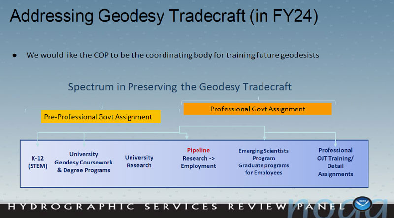
Besides providing funds for the geospatial grants, NGS is collaborating with other federal agencies to address the geodesy crisis. This collaboration, denoted as the “Geodesy Community of Practice (COP),” includes four agencies — NGS, National Geospatial-Intelligence Agency (NGA), National Aeronautics and Space Administration (NASA), and United States Geological Survey (USGS). The co-chairs of the group discussed the group’s actions and goals at the Hydrographic Services Review Panel (HSRP) fall committee meeting held in Silver Spring, Maryland, on Sept. 27-29.
Geodesy Community of Practice. (Image: NOAA’s Hydrographic Services Review Panel)
The HSRP involves four NOAA offices: three National Ocean Service (NOS) program offices -NGS, the Center for Operational Oceanographic Products and Services (CO-OPS), the Office of Coast Survey (CS), and the University of New Hampshire’s Joint Hydrographic Center and Center for Coastal and Ocean Mapping. More information and the presentations from the HSRP meeting can be obtained here. The purpose of the committee is to review and provide NOAA with independent advice on their products and services.
I attended the three-day HRSP meeting as a virtual participant. As previously noted, NGS is one of the NOS offices that’s part of the HSRP. As the Director of NGS, Blackwell participated in the 2023 fall HSRP meeting. A majority of the meeting discussed the geodesy crisis. In my opinion, this is due to Blackwell’s efforts to highlight the importance of geodesy to NOAA products and services.
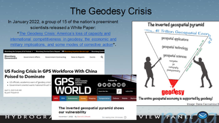
The presentation by the co-chairs of the Geodesy Community of Practice highlighted a few articles that have brought the geodesy crisis to the attention of the geospatial user community. Anyone keeping up with my columns knows that I have been highlighting the geodesy crisis and programs that advance the science of geodesy (July 2020, November 2022, December 2022, and April 2023). The geodesy crisis white paper is posted on the American Association for Geodetic Surveying (AAGS)website.
Image: NOAA’s Hydrographic Services Review Panel)
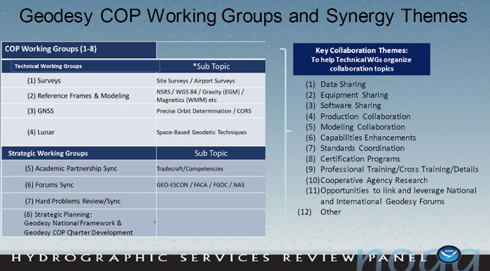
The Geodesy COP established working groups to address topics that are important to all geospatial users. All the agencies are supporting the working groups which should help create more effective and efficient solutions to technical geodetic issues.
Image: NOAA’s Hydrographic Services Review Panel
A goal of the Geodetic Community of Practice is to train future geodesists. The advancements in satellites and computers have enabled geodesy to expand into many different disciplines. Geodetic science and technology now underpin many sciences, large areas of engineering (such as driverless vehicles and UAVs), navigation, precision agriculture, smart cities, and location-based services.Major U.S. companies, such as Google and FedEx, as well as the automobile industry, precision farming companies and mining companies also need more accurate geodetic models, tools, and algorithms.Therefore, these companies also need trained geodesists to perform important research on topics that address their specific geodetic requirements.I highlighted this in my July 20, 2020, GPS World First Fix article.To address the geodesy tradecraft, the COP includes providing professional government assignments.That said, many industries that rely on accurate and consistent geodetic information should also provide professional geodetic assignments.
Training future geodesists. (Image: NOAA’s Hydrographic Services Review Panel)
I asked Blackwell how she thought the U.S. government’s Geodesy Community of Practice will help NGS and the geodesy crisis.
“The Geodesy Community of Practice is in the beginning phase right now with the collaboration among federal agencies with geodetic missions, NOAA/NGS, NGA, NASA, and USGS,” Blackwell said. “There is already a benefit in sharing research, workforce, and operational needs and leveraging our resources. I envision expanded engagement with academia, private industry, and other government agencies as the community of practice matures.”
In my opinion, the Geodesy Community of Practice’s integrated working groups consisting of individuals with different backgrounds and skills addressing geospatial problems will help to advance the field of geodesy. I believe that integrated and collaborative organizations create the best geospatial solutions; the Geodesy COP is an embodiment of this concept.
Of course, as I have stated in many of my columns, I like to remind everyone that “geodesy is the foundation for all geospatial products and services.”
NV5 Geospatial, a large geospatial data company, provides services for airport projects across the United States and U.S. territories — mainly supporting airport planning and engineering firms that must meet FAA survey and mapping requirements for data collection at airports. “We generally are a sub-consultant to them, helping them achieve those survey standards for collecting the data and submitting it to the FAA,” said David Grigg, the company’s Aviation Program Director. Typically, this is around planning projects such as airport layout plans and master plans, but also engineering projects such as runway extensions and runway reconstructions.
As an example, Grigg cited the extension of a runway, which requires new flight procedures to be established. “Two survey missions are required for runway extensions. The primary mission is to establish control for the aerial imagery. Using the imagery, control and design data, we check for obstacles photogrammetrically. That data is sent to the FAA and procedures are developed. After construction is complete, we go back to the airport to survey the changed runway and navigational aids (NAVAIDS) to verify that what was designed was ultimately built.”
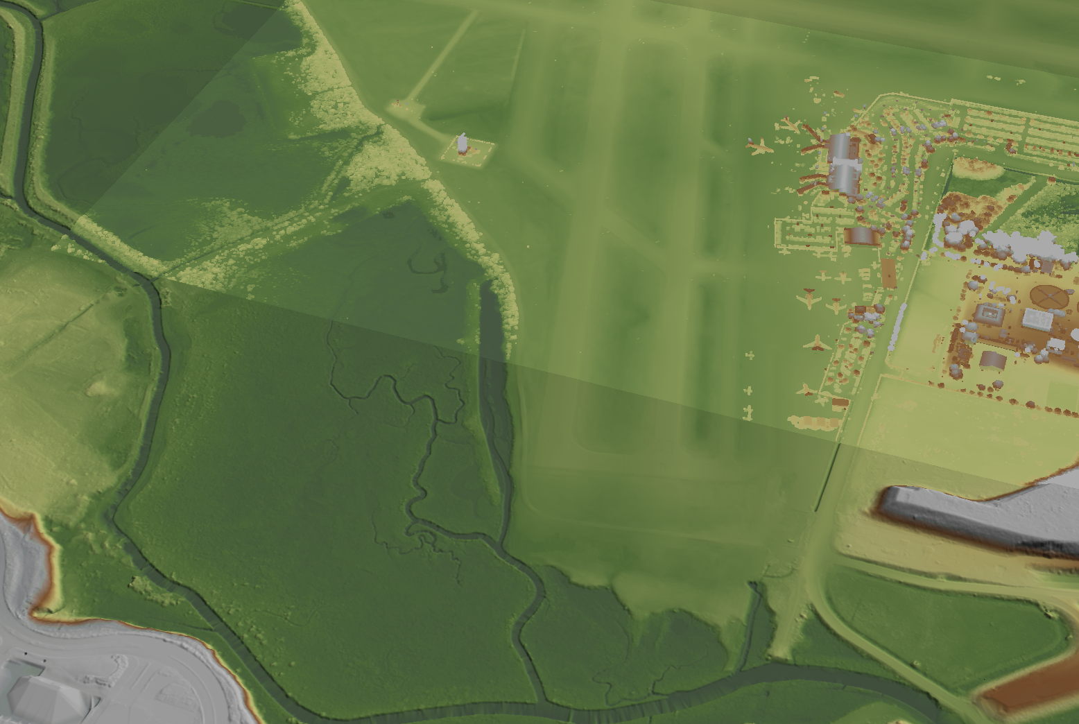
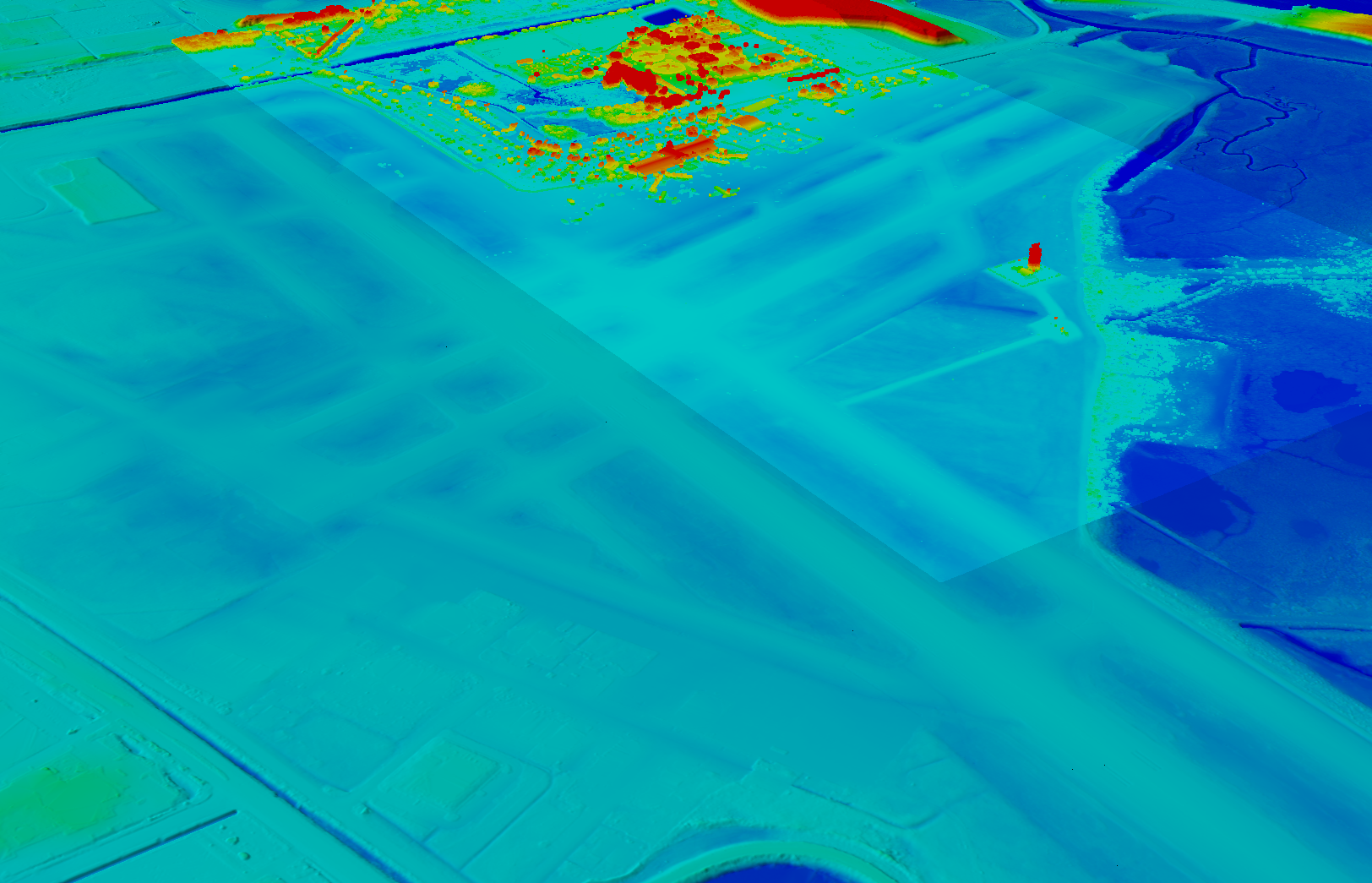
Another way in which NV5 Geospatial supports airport clients is by conducting obstruction studies around them for vegetation management. “That’s generally where we pull in the lidar surveys,” said Grigg. The FAA’s standards for relative and absolute positioning accuracy for trees are “rather generous” by surveying standards, he said. “We’re talking two to three feet vertically and twenty feet horizontally. It’s not like a typical mapping job where you’re guaranteeing it to one foot or better horizontally and half foot or better vertically.”
The FAA, he points out, has published guidance on how lidar may be used. “We mostly use aerial photogrammetry to support projects in the FAA’s airports GIS program. When we collect lidar at an airport, we do it to generate contours and to identify individual tree canopies. Our lidar-derived data is most often developed to benefit airports for tree mitigation not for FAA airports GIS survey projects.”
Image: NV5 Geospatial
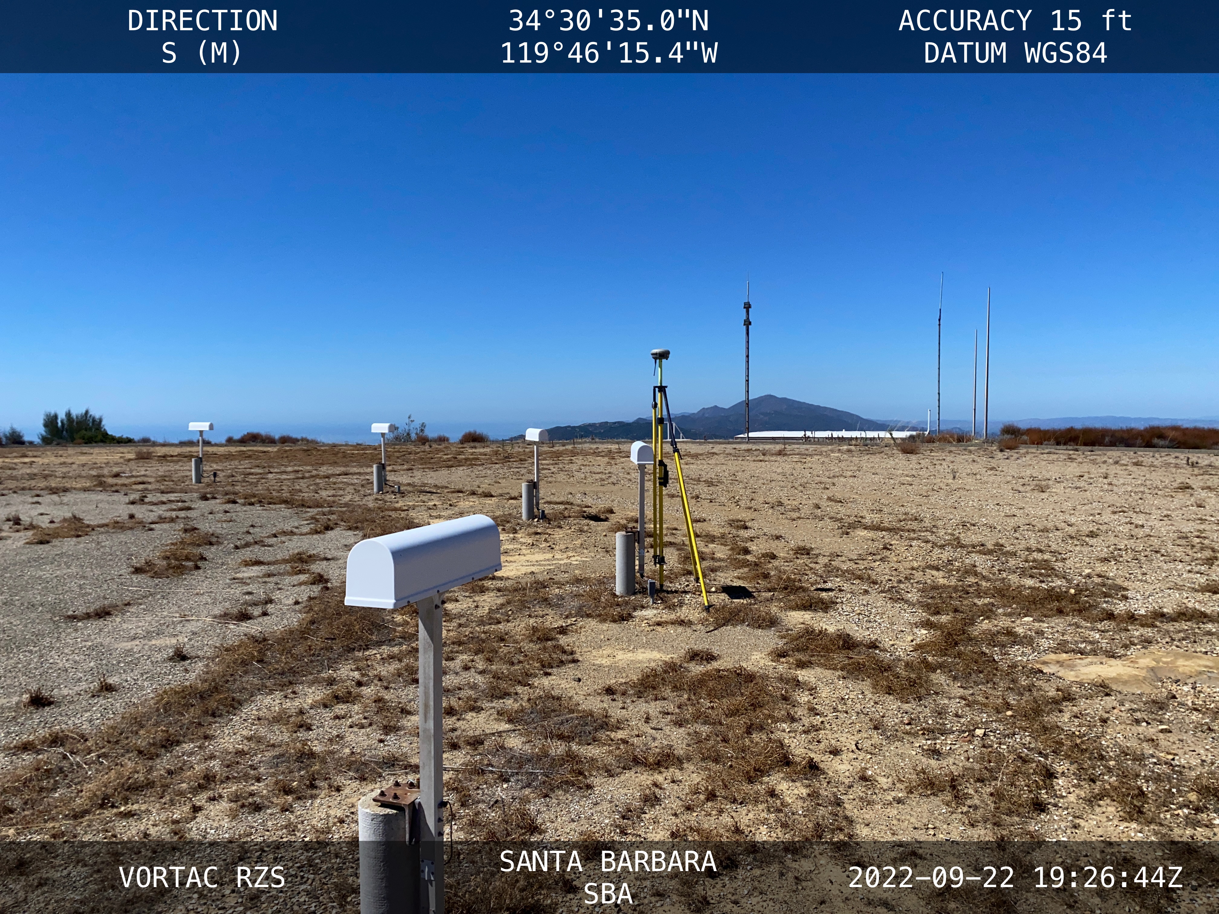
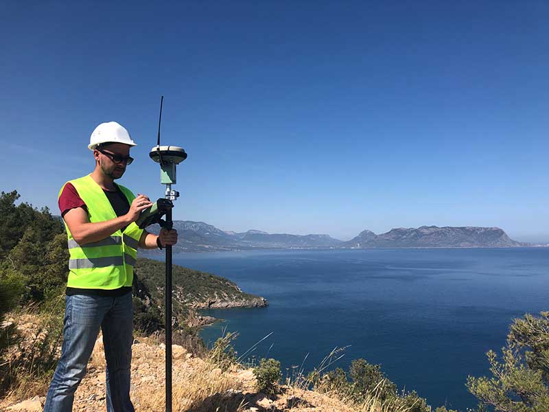
On the other hand, the FAA has strict requirements regarding metadata to document when, where, and how each control point is collected. “At the time of the survey, photographs are taken of the GPS units from different angles and cardinal directions,” Grigg said. “This is visual documentation for NGS that the surveyed point is at the location described. ”
Another challenge for surveyors working at airports is that they are required to pull back for incoming aircraft. “Obviously, you will have some logistical issues at busy airports,” said Grigg. Surveyors are required to have special lights and markings on any vehicles that enter the airport property to ensure ground and air visibility. Aircraft movement also impacts surveyors as they must move away from the runway safety area (RSA) for take-offs and landings. Busier airports are surveyed at night, when air traffic is reduced or runways are closed.
Image: NV5 Geospatial
A typical project for a small airport takes about nine months, while for bigger airports — such as Chicago O’Hare, Dallas-Fort Worth, or Hartsfield-Jackson Atlanta — they can take up to twice as long. “The large hubs update their master plan on a more reoccurring basis, such as every three to five years,” said Doug Fuller, NV5 Geospatial’s Airport Solutions Specialist. “As the airports get smaller, you start stretching out that timeframe.”
Airport survey requirements
[The following was written by NV5 Geospatial and only lightly edited by GPS World.]
Airports have surveys conducted for many different reasons. However, all survey types require the collection, classification and reporting of accurate data about the project. The methodology selected to gather the information is up to the professional surveyor’s judgment. Some features require observation through ground field methods, while others lend themselves to collection via remote sensing technologies.
All surveys start with a search for existing airport control, which are called Primary Airport Control Points (PACS) and Secondary Airport Control Points (SACS). These are points on the airport that have been adjusted by the National Geodetic Survey (NGS). This ensures that the survey is done on the National Spatial Reference System (NSRS).
A typical survey includes surveying the runway, the end points, any displaced thresholds, and a profile along the centerline of the runway. If the centerline marker is not in the correct location or if it is not there at all, the surveyor will make the necessary measurements to establish the proper location and set a new marker. Next the surveyor must locate all NAVAIDS and survey them at the proper location as described in FAA Advisory Circular 150/5300-18B.
After the NAVAIDS are located, the photo control survey will be done. This still requires the PACS and SACS to be the points of origin of the survey. The base requirement as described in FAA Advisory Circular 150/5300-16C is to survey ten photo control points and five check points. The check points are sent to NGS’s Online Positioning User Service (OPUS). This is used to check that the survey was done on the NSRS and that the compilation meets FAA standards.
The standards the surveyor must meet vary depending on the equipment type or photo control point. Examples of the accuracy requirements for the NAVAIDS are as follows:
Point
Horizontal
Vertical
Distance measuring equipment
+/- 1 ft
+/- 1 ft
Glideslope
+/- 1 ft
+/- 0.25 ft
Inner marker
+/- 10 ft
+/- 20 ft
Localizer
+/- 1 ft
+/- 0.25 ft
Runway end point
+/- 1 f ft
+/- 0.25 ft
Runway profile points
+/- 1 f ft
+/- 0.25 ft
Photo control
+/- 1 ft
+/- 1 ft
PACS and SACS
X
Y
Z
Ellip.
Inverse from PACS to SACS
surveyed relative to published
0.09 ft
0.09 ft
0.15 ft
0.13 ft
When surveying on airport property, the largest challenge is always accessing the runway safety area to locate the runway ends and profiles. At small airports Surveyors must work when the runway is not busy; at airports with FAA control towers when the runway is closed. Frequently this is done overnight. Other challenges include access to the FAA NAVAIDS. Some of them must be turned off to be surveyed and others require survey points on which it is not possible to set an instrument. When we are not able to occupy a point, we collect it by surveying multiple equidistant locations around the NAVAID and averaging them.
Image: NV5 Geospatial
NV5 Geospatial surveyors use a combination of real-time (R/T) and post-processing techniques. We also use OPUS with the PACS and SACS and the five check points. Once the PACS and SACS have been determined to be stable, the proper coordinates are applied to them and the R/T points are adjusted using Trimble Business Center (TBC). NV5 Geospatial uses Trimble TRM-R8s and we recently added TRM-R12i receivers to our equipment. We use ground control points to orient the photography and to calibrate the lidar.
Last month’s column highlighted GEO-ESCON and how it supported the advancement of the science of geodesy. That said, the National Geodetic Survey (NGS) has been working to improve the National Spatial Reference System (NSRS) by replacing the North American Datum of 1983 (NAD 83) frame and all vertical datums, including the North American Vertical Datum of 1988 (NAVD 88), with four new terrestrial reference frames and a geopotential datum. Many of my previous GPS Worldcolumns have addressed various phases of the project.
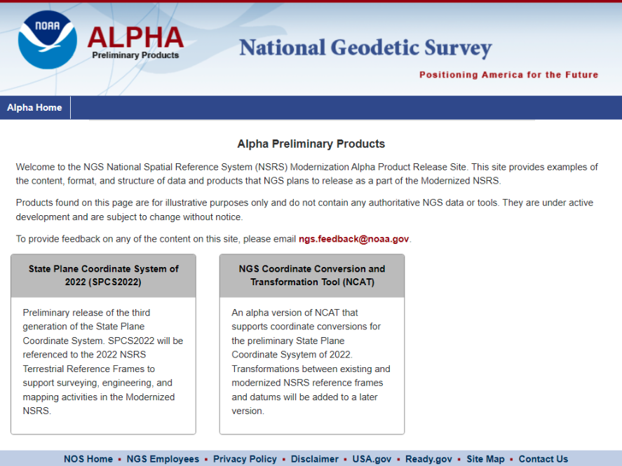
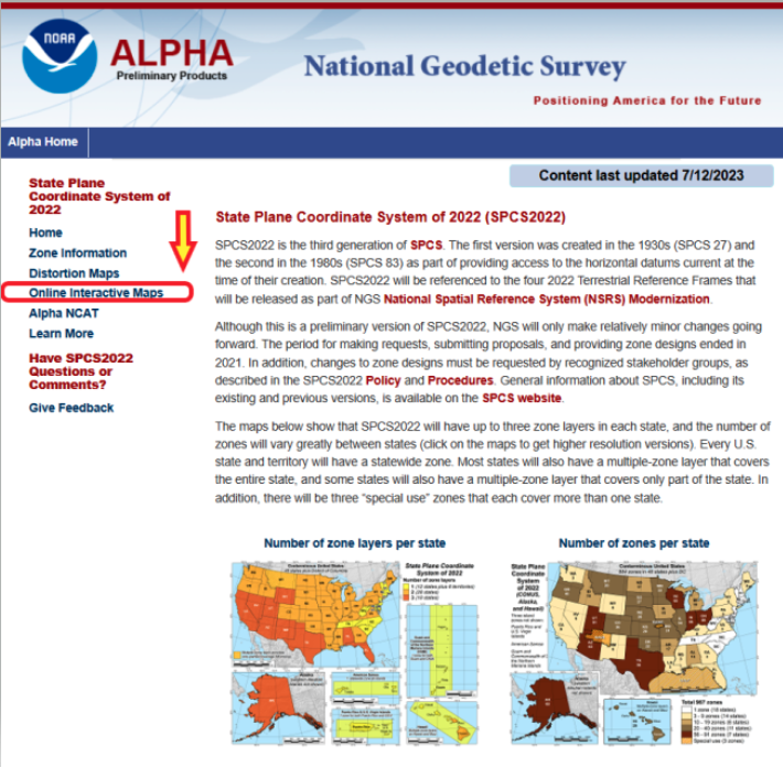
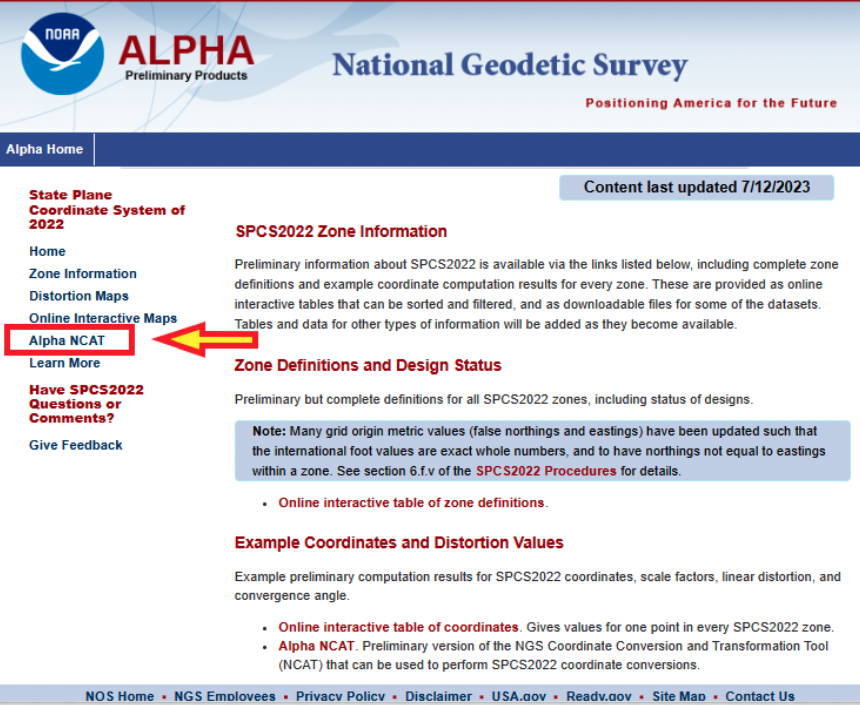
Recently, NGS has developed an Alpha site to enable users to preview preliminary NSRS products and services. I mentioned the Alpha site in my July column, in which I highlighted NGS’s presentations on the new NSRS at the International 2023 FIG Working Week.
Alpha preliminary products page. (Image: NGS)
The concept of the Alpha site is to provide examples of the content, format, and structure of data and products that NGS plans to release as a part of the modernized NSRS.
NGS highlights that these products are for illustrative purposes only and do not contain any authoritative NGS data or tools. It states that they are under active development and are subject to change without notice.
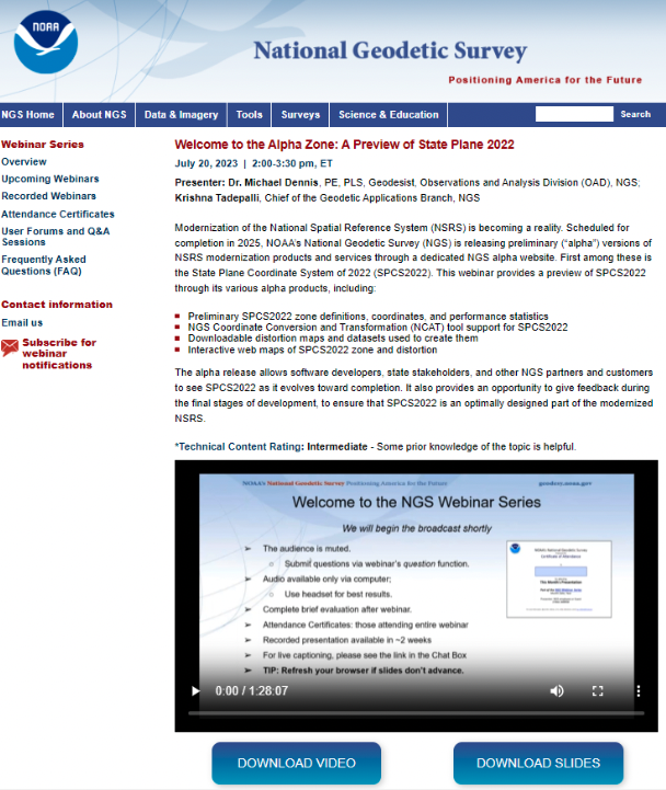
That said, NGS would like everyone to try the Alpha products and provide feedback to NGS. The first two Alpha products are State Plane Coordinate System of 2022 (SPCS2022) and NGS Coordinate Conversion and Transformation Tool (NCAT). On July 20, NGS held a webinar previewing the Alpha site. Readers can download the powerpoint and video of the presentation here.
Webinar on preview of SPCS2022. (Image: NGS)
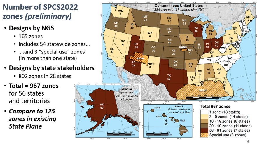
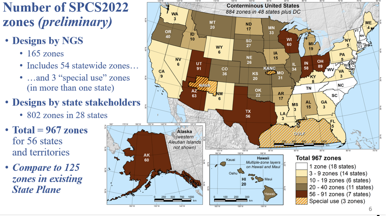
As usual, Michael Dennis of NGS did a great job of describing the new SPCS2022, and the differences between the State Plane Coordinate System of 1983 (SPCS83) and SPCS2022. I have included a few of his slides that highlight the SPCS2022.
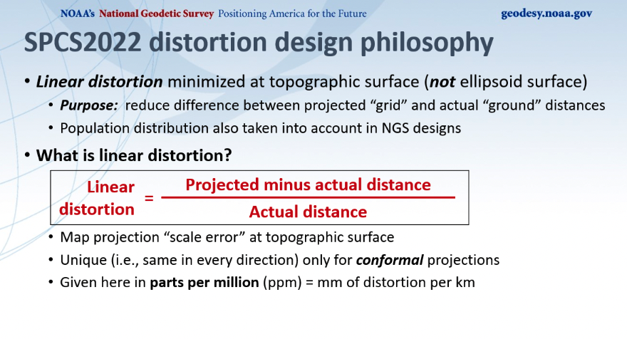
First, SPCS2022 has significantly more zones than the current SPCS83 zones. Second, SPCS83 map projections were designed to minimize linear distortion at ellipsoid surface, whereas the SPCS2022 map projections were designed to minimize linear distortion at topographic surface. The purpose being to reduce the difference between projected “grid” and “actual” ground distances.
Number of SPCS2022 zones. (Image: NGS)Linear distortion of SPCS2022. (Image: NGS)
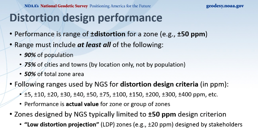
Dennis described NGS’s distortion design performance as seen in the image below. He explained that the performance is a range of +/- distortion for a zone, such as +/-50 ppm. The analysis involved determining parameters where the range includes 90% of the population, 75% of the cities and towns, and 50% of the total area. He highlighted those zones designed by NGS that where typically limited to +/- 50 ppm design criteria, but many low distortion projections (LDP) zones designed by stakeholders consisted of +/- 20 ppm design criteria.
Distortion design performance. (Image: NGS)
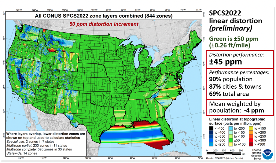
Dennis provided a slide depicting SPCS2022 linear distortion for all CONUS zones with a 50 ppm distortion increment as seen below. As indicated on the slide, green is +/- 50 ppm. The distortion performance is +/- 45 ppm.
All CONUS SPCS2022 zone layers. (Image: NGS)
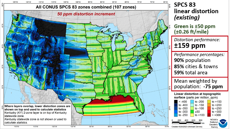
As a comparison to the existing SPCS83 zones, he provided a similar slide for the CONUS SPCS83 zones. See below. As in the previous slide, green represents +/- 50 ppm. The distortion performance is +/- 159 ppm.
All CONUS SPCS83 zone layers. (Image: NGS)
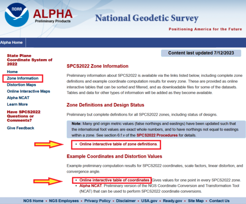
Now, let us look at the Alpha products. First, all zone information can be found here.
SPCS2022 zone information. (Image: NGS)
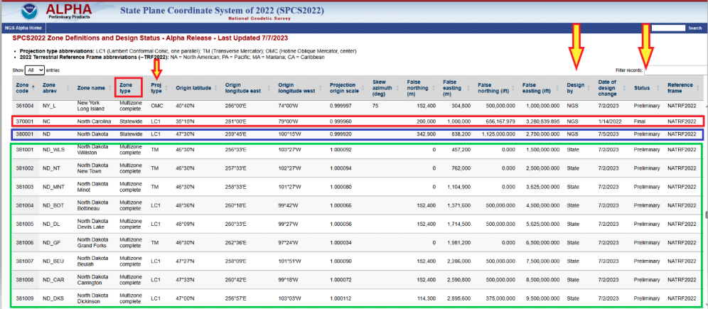
Users can click on the image below for a table of all zone definitions. The table provides the type of projection, if it was designed by NGS or the state, and the zone definition.
Online interactive table of zone definitions. (Image: NGS)
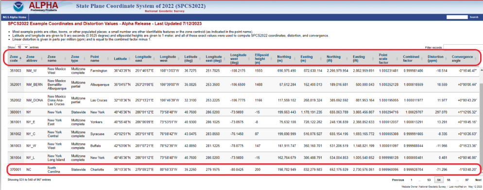
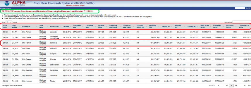
By clicking on the image below, users can obtain information for a point in a particular zone. The table provides northing and easting (meters and feet), scale factor, linear distortion, and convergence angle for a specific coordinate in a particular zone. It should be noted that all values that are provided in feet will be international feet units (ift).
SPCS2022 example of coordinates and distortion values. (Image: NGS)
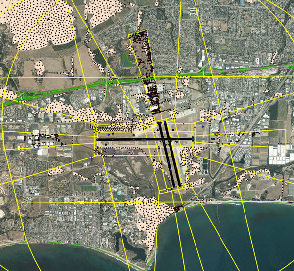
The Alpha page provides an online option to look at all maps. The arrow in the image below highlights the link to access the online interactive maps.
Alpha page for SPCS2022. (Image: NGS)
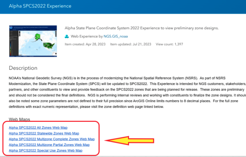
When users click the link on the page, they are directed to an ArcGIS NOAA web map viewer.
Alpha SPCS2022 experience. (Image: NGS)
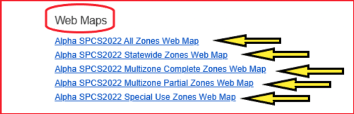
To access the online map function, users need to click one of the Alpha SPCS2022 zone options.
Alpha web maps. (Image: NGS)
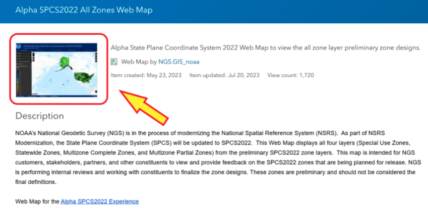
Once users click on one of the web map buttons, another map page with a map icon appears on which userswill need to click to get to the map of zones.
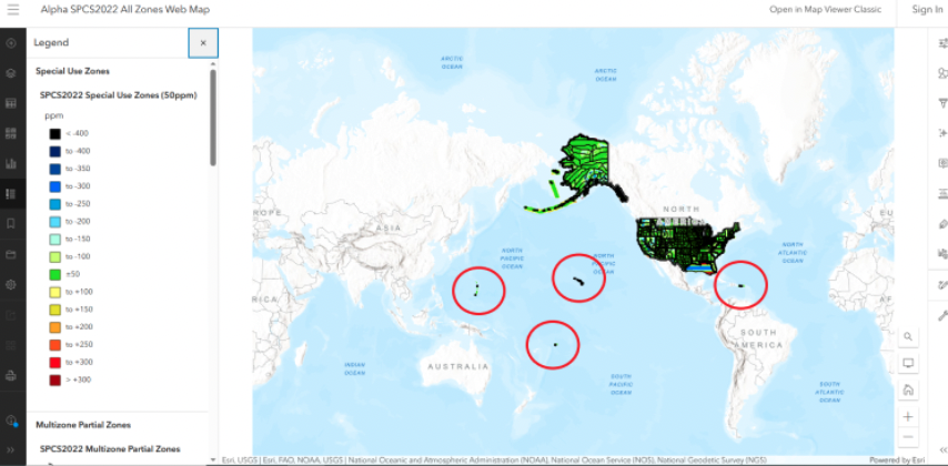
Alpha SPCS2022 all zone web map. (Image: NGS)
After users click on the map icon, they will get another web page that contains the map zones based on their selection. In my example, I selected “all zone web map.” Once users get to this page, they can zoom into any area to find a particular zone.
All zone web map. (Image: NGS)
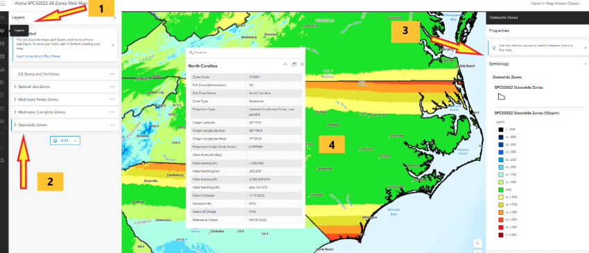
I zoomed down until I located North Carolina’s map zone. The web page provides access to various layers and information. First, if users move their curser over the layer button, a list of layers pops up. Next, select one of the layers, such as Statewide Zones, then the properties of the map are placed on the map. Finally, when readers click on the map itself, the information about the SPCS2022 zone appears on the map.
Alpha North Carolina Statewide Zone web map. (Image: NGS)
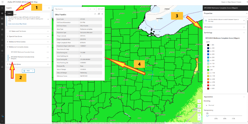
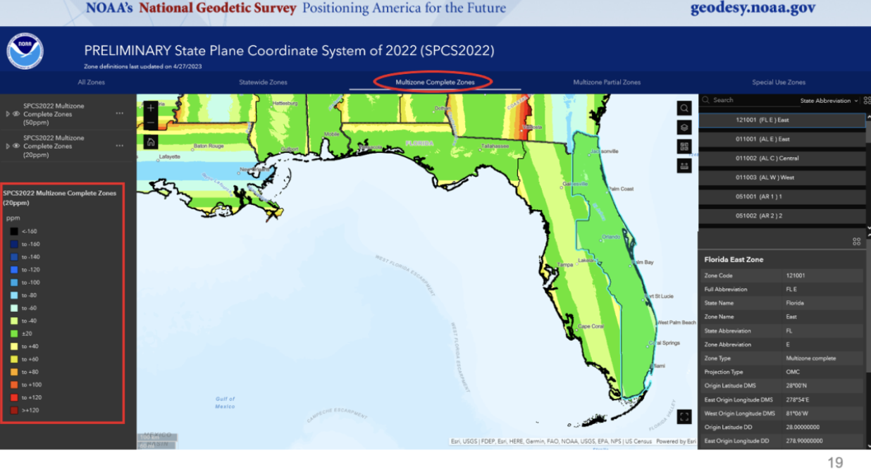
North Carolina is a state that elected to have a single statewide zone. Some states decided to design several LDPs that cover certain areas or cover the entire state. Ohio is a state that designed 89 LDPs that cover the entire state. Again, by selecting the layer button, users have an option to select multizone complete zones, the properties appear on the map, and finally clicking on the map provides the zone information for that zone. In this example, I clicked on Columbus, Ohio, which is in the Ohio Franklin Zone.
Alpha Ohio multizone complete zones web map. (Image: NGS)
Users can obtain specific information for a coordinate located in the Ohio Franklin Zone by clicking on the online interactive table of coordinates. Note that the distortion is 6.725 ppm at the coordinate in the zone.As previously stated, this was a user–defined LDP zone.
SPCS2022 example of coordinates and distortion values in Ohio Franklin Zone. (Image: NGS)
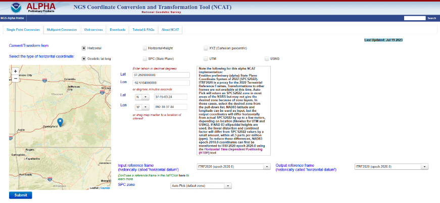
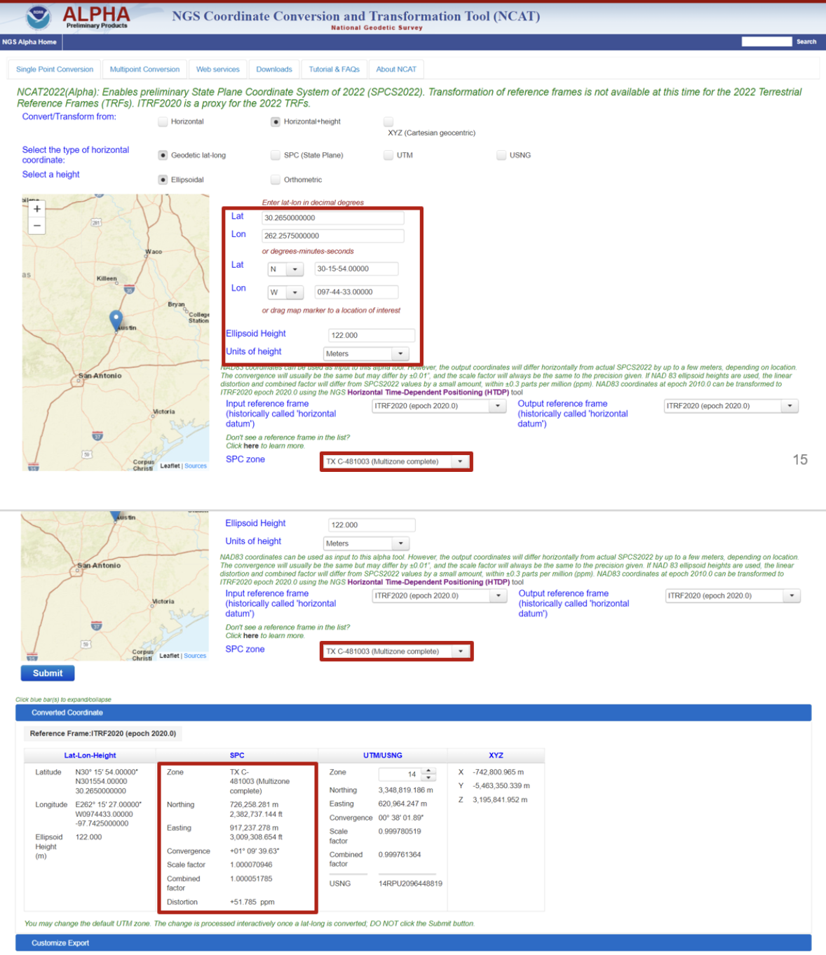
Another Alpha site available for users to evaluate is the NGS Coordinate Conversion and Transformation Tool (NCAT). NCAT is probably the tool that most surveyors will be interested in using and providing feedback to NGS. Users can access NCAT on the Alpha SPCS2022 webpage or by clicking here.
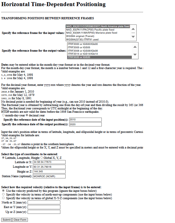
The Alpha NCAT website has a note about the coordinates that users should provide as input to the routine. The bottom line is that the input coordinates need to be in ITRF2020 (epoch 2020.0), or readers may not get their desired zone. NGS recommends that users convert the coordinates to ITRF2020 (epoch 2020.0) using the Horizontal Time-Dependent Positioning (HTDP) tool.
Users can access HTDP here. I provided an example of HTDP for a CORS in North Carolina. I used the NAD 83 (2011) [epoch 2010.0] published coordinates of the CORS as my input values.
Example of a HTDP computation. (Image: NGS)Output of a HTDP computation. (Image: NGS website)
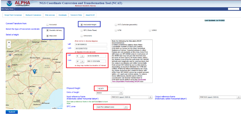
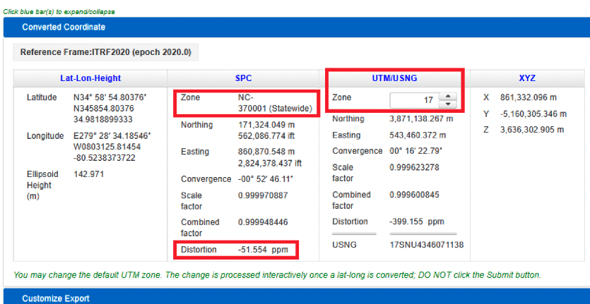
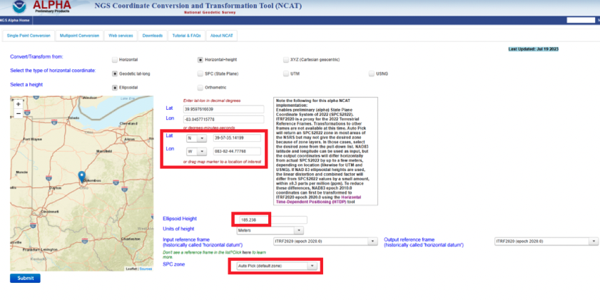
After using HTDP to transform the coordinates from NAD 83 (2011) to ITRF2020, I used the Alpha NCAT tool to compute the SPCS2022 values for the mark. I provided an example of the Alpha NCAT routine using the coordinates of the North Carolina CORS NCMR. The program defaults to horizontal only, so I changed it to the horizontal-height option. The user then enters the latitude, longitude, and height of the mark. Lastly, the user has an option to select the SPC zone or the program will select the zone based on the coordinates of the mark. In my example, I selected the auto pick option.
NCAT input for MONROE CORS (NCMR). (Image: NGS)
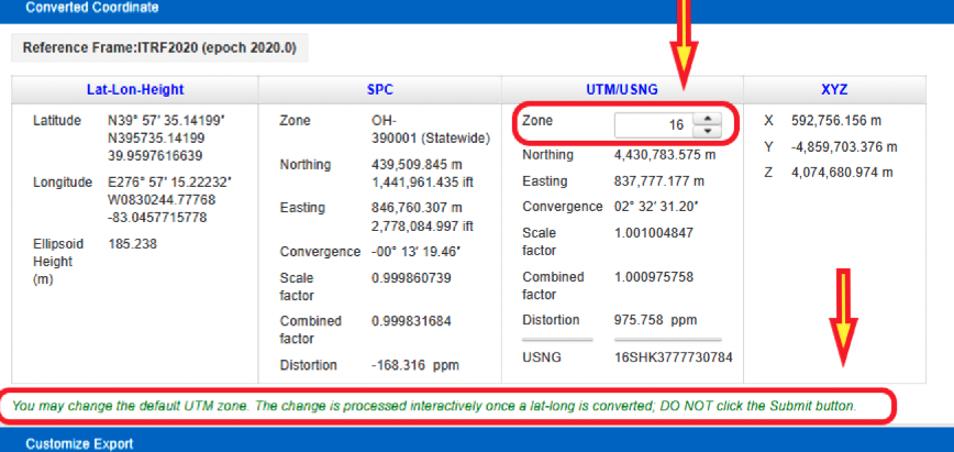
The image below provides the output of NCAT. I have highlighted a few items in the image. First, the program selected North Carolina’s Statewide Zone, the distortion is -54.554 ppm at this mark, and the UTM zone selected is Zone 17. The output also provides the scale and combined factors.
NCAT output for NCMR. (Image: NGS)
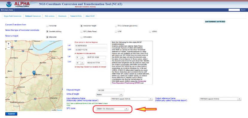
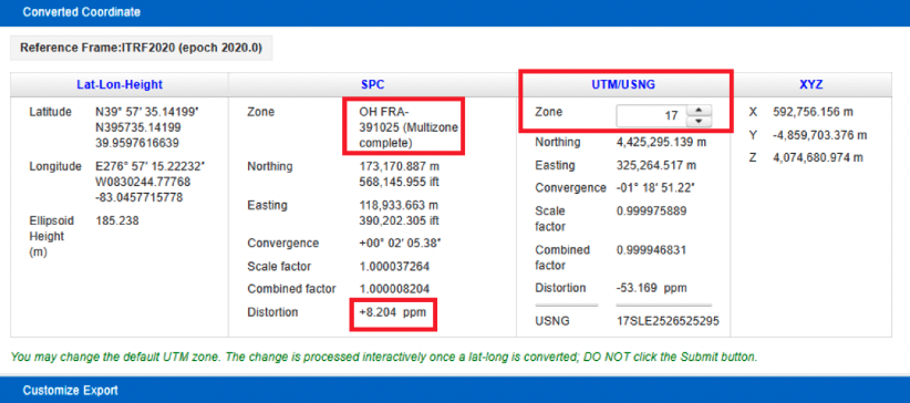
North Carolina is a state that elected to have a single statewide zone, but, as previously mentioned, some states decided to design their own LDPs. Again, Ohio is a state that designed LDPs that cover the entire state. Once again, I entered the coordinates into the input boxes and selected the auto pick (default zone) option. As indicated in the converted coordinates section, the program selected the OH FRA-391025 zone based on the coordinates of the mark. Notice that the distortion is only +8.024 ppm.
NCAT results for Columbus CORS (COLB). (Image) NGS)
The user has the option to select a different zone than the default zone. The image below provides the SPC values for the COLB mark when selecting the Ohio Statewide Zone. Notice that the distortion value changes from +8.024 ppm to -168.316 ppm. Also, as expected, the UTM and X, Y, and Z values have not changed.
NCAT results for COLB selecting Statewide Zone. (Image: NGS)
One last option to highlight is that the user can change the default UTM zone by clicking on the up or down arrows under the UTM column. In my example, I changed the UTM zone from 17 to 16. Obviously, the values under the UTM column changed.
Option to change default UTM zone. (Image: NGS)
The concept of the NGS’s Alpha site is to provide examples of the content, format, and structure of data and products that NGS plans to release as part of the modernized NSRS. NGS states that these Alpha products are for illustrative purposes only and do not contain any authoritative NGS data or tools. It states that they are under active development and are subject to change without notice.
That said, NGS would like everyone to try these Alpha products and provide feedback to NGS, so that they can improve their products and services. I would encourage readers to try these Alpha sites and provide comments and suggestions to NGS.
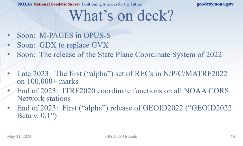
Anyone reading my previous columns knows that I have been highlighting the new, modernized, National Spatial Reference System (NSRS) of the National Geodetic Survey (NGS). During the 2023 Fédération Internationale des Géomètres (FIG) Working Week held on May 28 – June 30, in Orlando, Florida, NGS held an all-day session addressing various topics related to the NSRS modernization project.
More than 30 NGS staff members supported two days of sessions that included a day on the NSRS modernization, sessions for the Young Surveyors Network, and FIG Commission 5 meetings, which focused on meeting the highest accuracy levels for positioning and measurement.
Juliana Blackwell, director of NGS, kicked off the third plenary session tackling the global challenges, with a presentation titled “The Modernized U.S. National Spatial Reference System — Aligning National Geospatial Data to the Globe.”
Blackwell highlighted the importance of geospatial data from many different sources being interoperable and defined within a modern reference frame. She noted that NGS is part of the National Oceanic and Atmospheric Administration (NOAA), the mission of which is to understand and predict changes in climate, weather, ocean, and coasts. This includes a mandate to define, maintain and provide access to the NSRS.
NGS’s NSRS modernization project has been underway for a decade and is nearly complete. Blackwell explained that the new NSRS will align critical U.S. geospatial data assets within global data inventories and enable improved analysis and modeling of climate changes and impacts to society and the environment. The modernized NSRS will enable data integration of new and old technologies, adopts modern standards, and empowers growth in new fields and applications.
The remainder of the presentations during the all-day event covered three themes: the practical implications of NSRS modernization — changing survey methodology; an update on the NOAA CORS Network and the Online Positioning User Service (OPUS); and case studies of surveys — what NGS does now and how they will change.
Many of these topics have been discussed by NGS during their webinar series, but during these presentations NGS provided the latest information on many of the activities associated with the modernization of the NSRS. This venue allowed for participants to ask questions as opposed to typing them in a box. Also, the NGS employees that participated in the FIG working week were available for discussions before and after the session. I enjoyed my discussions with old colleagues as well as meeting some new NGS employees.
The session titled “Practical Implications of NSRS Modernization — Changing Survey Methodology” addressed the following topics:
practical impacts of the modernized NSRS
Canada’s implementation of the modernized frames
changes afoot: State Plane 2022 and Retirement of the U.S. Survey Foot and
preparing for the modernization of the NSRS.
Dru Smith, NSRS modernization manager, started by explaining the practical impact of the modernized NSRS and why it is needed. He mentioned that the current NSRS was defined in the pre-GNSS era and that it has failed to keep up with emerging requirements, such as accurately measuring sea level rise.
(Image: NGS Website)
He highlighted the practical implications of the modernized NSRS, such as that every latitude, longitude, and ellipsoid height will change from its NAD 83 values in the +/-2-meter range, and every orthometric height will change from its NAVD 88 values in the +/-2-meters median range.
He mentioned that the published coordinate functions of the NOAA CORS Network (NCN) will be the primary geodetic control of the NSRS. He noted that NGS is working on the integration of web-based tools to improve consistency and reduce confusion, such as enhancements to NGS’s OPUS to ingest digital data from surveying instruments directly into OPUS 6 via a Geodetic Data Exchange (GDX) format. This would include raw measurements from GNSS receivers, levels, total stations, and gravimeters. The talk titled “Augmenting Data Exchange Formats for OPUS of the Future” by Ryan Hardy, discussed the GDX format in more detail.
As with the International Terrestrial Reference Frame, the modernized NSRS will have a time-dependency component. It will be built into the new NSRS, but users will have the ability to disengage from it.
Smith provided a timeline of the project for the next couple of years, which can be referenced in the image below. NGS plans to release data and support tools on their BETA website during 2024 and 2025.
(Image: NGS Website)
Smith discussed how some products will be released early for users to test and evaluate how the new NSRS products will affect their products and services, and to be ready for their customers after the new NSRS is released for publication. Products scheduled for early releases (Alpha Release), include SPCS2022, EPP2022, and GEOID2022.
He emphasized that Alpha products, by definition, can be one or more of the following:
incomplete
inaccurate
buggy
subject to change without notice
As such, their early release is primarily for users to see the “big picture” such as formats of data and the general direction that NGS is taking.
He provided a list of new products that will be announced soon, and some alpha products tentatively planned for release in 2023.
(Image: NGS Website)
Michael Dennis did a nice job of discussing the State Plane Coordinate System of 2022 (SPCS 2022) and the retirement of the U.S. Survey Foot. He mentioned that the U.S. Survey Foot was superseded by the international foot on December 31, 2022. His presentation gave a brief overview on the status and rollout plans for SPCS2022, along with how and why NGS will continue to support the U.S. Survey Foot in the existing NSRS (but not in the modernized NSRS).
See the image below for the number of zones for each state.
(Image: NGS Website)
The SPCS2022 will be an alpha product released soon. Part of the alpha product will have options to view maps depicting the different zones in each state.
Example of Florida Multizone Complete Zones. (Image: NGS Website)
When NCAT2022 is released in alpha product it will contain the SPCS2022.
Example of NCAT2022 (Alpha). (Image: NGS Website)
Representatives from the Canadian Geodetic Survey presented and participated in the discussions.
The session titled “Update on the NOAA CORS Network and OPUS” addressed the following topics:
the NOAA CORS Network (NCN) services
updating OPUS-S to support multi-GNSS
OPUS -Projects 5: supporting RTK for establishment of geodetic control
OPUS projects for manager’s training – transitioning from instructor-led to online, self-paced instruction and
augmenting data exchange formats for OPUS of the future.
Dan Gillins gave a presentation on the advantages of using NGS’s OPUS-Projects 5 web routine. OPUS-Projects make it easier for users to submit a GNSS project to NGS for publication. I discussed OPUS-Project 5.1, when it was released as a Beta product, in my October 2021 column.
(Image: NGS Website)(Image: NGS Website)
Gillins mentioned that a new publication providing guidance to meet standards for GNSS surveying is being reviewed and will be available soon. I discussed these new standards in my May 2023 column.
Ryan A. Hardy gave a talk describing the new Geodetic Data Exchange (GDX). As previously mentioned, GDX is an XML-based data format that will be the input format for OPUS. GDX will be the successor to the GNSS Vector Exchange (GVX) format. GDX currently supports GNSS, classical, and leveling measurements.
The GDX structure will have the following fields[[these are clearly the names of database fields; if it were a list of different types of information, we would not put them in all caps and would not use the underscores]]:
SOURCE_DATA
PROJECT_INFORMATION
PERSONNEL
UNITS
EQUIPMENT
POINTS
MEASUREMENT_SETTINGS
MEASUREMENTS
REDUCTIONS
OBSERVATIONS
NGS is planning to release an alpha version of GDX soon.
(Image: NGS Website)
The session titled “Case Studies of Surveys — NGS Does Now and How They will Change” addressed the following topics:
implementing NGS OPUS-Projects’ GVX feature to align RTK vectors to the NSRS to establish geodetic control for FirstNet indoor mapping
IGLD: a case study for leveraging digital tools to enhance QA/QC on large scale static GNSS observation campaigns
geodetic leveling in the modernized NSRS and
NGS field operations: modernizing in many ways.
Ben Erickson gave a good presentation on leveling in the new NSRS, a topic about which I am very interested in knowing more[[Please avoid dangling participles, prepositions, conjunctions, and modifiers.]]. I discussed the new procedures in my June 2020 column.
One major change is that leveling surveys will require GNSS occupations to ensure that orthometric heights computed in leveling surveys are up to date and are connected to the NSRS through the NOAA CORS Network. The network accuracy is obtained through GNSS data and a high-accuracy geoid model, and the local accuracy is provided through the leveling data. Specific procedures will be required to incorporate leveling data in the North American Pacific Geopotential Datum (NAPGD2022).
Basic Procedures for NAPGD2022 Orthometric Heights. (Image: NGS Website)
I discussed these procedures in more detail in my June 2020 column. The image below provides a conceptual diagram that illustrates what this means to a typical leveling project.
GNSS + Leveling 2022 Procedures at the Start and End of the Leveling Project”. (Image: Diagram based on information from Dan Gillins, NGS, and modified by David B. Zilkoski)
Erickson provided a diagram of a level network that contained a loop, which can be referenced below.
(Image: NGS Website)
I have worked with leveling data for most of my career and I am pleased to know that NGS is going to provide tools to incorporate leveling data into the new, modernized NSRS. When performing leveling projects, there is a requirement to level to previously established benchmarks that were within a certain distance from the project. This helped to ensure that different leveling projects were consistent with each other. NGS stated that making adjacent projects at different epoch consistent is under development, and their plans include updating leveling documentation to explain the leveling methodologies and GNSS control.
(Image: NGS Website)
I have only highlighted a few of the presentations. It was an all-day session, and a lot of information was presented on the new, modernized NSRS. The presentations can be downloaded from the NGS website at https://geodesy.noaa.gov/datums/newdatums/fig-2023.shtml. I would encourage everyone to download the presentations to obtain the latest information on NGS’s modernization of the NSRS. See the image below for the list of presentations and the links to download specific presentations.
NGS Presentations at FIG 2023 Working Week. (Image: NGS Website)
On April 13, the National Geodetic Survey (NGS) held a webinar that described the classifications, accuracy standards and general specifications for GNSS geodetic control surveys using OPUS Projects. The webinar provided a summary of NOAA Technical Memorandum NOS NGS 92, which will be published after it has been through a final review. The presentation can be downloaded here and here. I will highlight some important sections of the webinar, but would also encourage readers to download it and watch it in its entirety.
NGS April 2023 Webinar (Credit: NGS Website)
As described in my March column, OPUS Project 5.1 routine now allows the use of RTN vectors and post-processed vectors from vender software. See my March column or NGS’ January 2023 webinar to learn more about OPUS Project 5.1.
The April webinar described the specifications that are required for GNSS surveys that will be submitted to NGS for publication. It was noted that these specifications are limited to the use of OPUS Project (version 5) for the establishment of North American Datum of 1983 (1983) coordinates and orthometric heights of vertical datums that are part of the current National Spatial Reference System (NSRS). The intent of the NOAA Technical Memorandum NOS NGS 92 is to replace NOAA Technical Memorandum NOS NGS 58 — “Guidelines for Establishing GPS-Derived Ellipsoid Heights, (Standards: 2 cm and 5 cm), Version 4.3” of November 1997, and NOAA Technical Memorandum NOS NGS 59 — “Guidelines for Establishing GPS-Derived Orthometric Heights” of March 2008.
Why replace the guidelines now?
First, there have been improvements in GNSS processing and technology since NOS NGS 58 was published in 1997. The guidelines did not consider the use of real-time kinematic (RTK) technology, the number of NOAA CORS has significantly increased since the 1990s, and NGS’ web-based software OPUS Project 5.1 now allows the use of RTN vectors and post-processed vectors from vender software. In my opinion, there is a difference between guidelines and specifications. Guidelines provide recommended procedures to meet a specific outcome or standard while specifications are an explicit set of requirements that need to be satisfied to meet a specific outcome or standard. In other words, guidelines are general recommendations, and by nature, should be open to interpretation and revised to meet new technological developments.
The webinar described the standards and specifications in 10 tables, which are displayed below. I will highlight a few of these tables that address how RTN vectors and post-processed vectors from vender software can be included in OPUS Project 5.1.
List of Tables:
Classifications of Network and Local Accuracy
Description of Mark Types and Anticipated Usage
Observation Method Requirements for Mark Types
Standards for Observation Requirements by Method
Standards for Network Design
Standards for Monumentation
Standards for Session Processing and Adjustment Results
Standards for Achieving Valid Orthometric Heights
Standards for Equipment Used in Field Observations and Office Procedures
Standards for Required Documentation
First, NGS has defined three classifications for network and local accuracies in Table 1 — primary, secondary and local. As expected, the accuracy values are different based on the classification. See Table 1. Table 4 provides the observation specifications for each classification.
Table 1. (Credit: NGS Website)
Table 2 provides definitions that are important to understand. NGS designates three different types of marks in the network design — NCN CORS, GVX base, and passive. See Table 2. Each of these types of marks has its own observation requirements which is described in Table 4.
Table 2. (Credit: NGS Website)
Information about the GVX vector format can be obtained here. Basically, the GNSS Vector Exchange provides a standard file format for exchanging GNSS vectors derived from varying GNSS survey methods and manufacturer hardware. NGS’s goal for developing GVX is to make it possible to upload vector data to OPUS-Projects. There are different observation specifications for OPUS Project processing GNSS data and for OPUS Projects accepting GNSS data observed and processed by manufacturer hardware and software — that is GVX data.
Please see my October 2021 column for more information on NGS’s GVX format.
A note on abbreviations: PP stands for post-processed; that is, OPUS PP are baselines processed in OPUS Project. GVX PP are baselines processed using a vendor’s software. GVX NRTK and SRTK are baselines from a vendor’s RTK systems.
Table 4 provides the observation requirements for primary, secondary, and local marks. I have highlighted the following items in that table:
All methods must repeat occupations and repeat sessions/occupations must be offset by 3 to 21 hours.
Required total static GNSS observation time for OPUS PP is greater than total static GNSS observation time for GVX PP data. That said, OPUS PP requires at least two sessions while GVX PP requires at least three sessions.
For GVX PP session, the duration of each session increases with distance and a GVX PP baseline cannot exceed 50 km (this is provided in Table 5:“Standards for Network Design”).
For GVX NRTK, the number of sessions increases to sixfor primary marks, the duration of occupations decreases to 5 minutes, a GVX NRTK baseline cannot exceed 40 km (this is provided in Table 5 – Standards for Network Design), and the mark requires at least three occupations on different days.
The use of GVX SRTK is not permitted for primary marks.
Table 4. (Credit: NGS Website)
Table 5 provides the specifications for network design; that is, the number of NOAA CORS required and the allowable distance from the HUB CORS. The image titled “Project includes 3 or more NCN CORS” provides a depiction of the specifications.
Table 5. (Credit: NGS Website)
Not all CORS are created equal, so users should evaluate the CORS they plan to include in their GNSS project. My December 2021 column discusses using NGS Map service to evaluate CORS data and plots. Some of the criteria that are used to evaluate CORS include the following: designated as “operational,” computed (measured) velocities rather than modeled (predicted) velocities, “consistent” data depicted in short-term time-series plots, network accuracies ~1 cm to 1.5 cm horizontally and less than ~2 cm to 3 cm in ellipsoid height.
Project includes 3 or more NCN CORS. (Credit: NGS Website)
Specifications for GVX vectors are also provided in Table 5. As indicated in Table 5 and previously stated, GVX PP baselines are limited to 50 km and GVX NRTK vectors are limited to 40 km.
Table 5 continued. (Credit: NGS Website)
An important specification that needs to be highlighted is that the maximum number of vector steps in a vector chain is two. This means there can only be one OPUS PP plus one GVX vector (either GVX PP or GVX RTK) in a vector chain. This is demonstrated in an example in theimage below.Also, specification 5.4 states that if GVX vectors are uploaded to the project, then a project needs one or more OPUS PP verified passive marks as checkpoints (these are denoted as GVX Validation Stations). The checkpoint marks have been highlighted in the image below as well.
NETWORK 4A – Submittable to NGS. (Credit: NGS Website)
If your state has many CORS with an NRTK, as North Carolina does, then the image below provides an example of how OPUS projects and GVX vectors can be used to efficiently and effectively establish primary control marks.
NETWORK 8A – submittable to NGS (Credit: NGS Website)
Table 7 provides session processing and adjustment results. The achieved network standard highlighted in the image is the same as the classification standard provided in Table 1, which is what should be expected.
Table 7. (Credit: NGS Website)
The maximum residual values in dN, dE, and dU are also provided in Table 7. This requirement is important because it helps to ensure that outliers are detected and removed, especially in the height component.
Table 7 continued. (Credit: NGS Website)
The webinar also had tables and diagrams for establishing orthometric heights. Table 8 and Figure 12 from the webinar provide a summary of the specifications. My January column described the specifications for establishing vertical control in the NSRS in more detail.
Figure 12 from the webinar. (Credit: NGS Website)
The image below describes specification 8.3 in Table 8. It is important to recognize that the marks that will be used as vertical constraints need to be observed for twoto six hours depending their distance from newly established marks.
Allowable distance to vertical constraints to achieve orthometric height. (Credit: NGS Website)
A lot of information was presented at the webinar and I only highlighted some important sections of it in this column. I would encourage everyone to download the webinar and watch it in its entirety. It should also be noted that NOAA Technical Memorandum NOS NGS 92 is in draft status and is awaiting several final approvals before it is made available for public comment.That said, the webinar’s contents are subject to minor changes as NGS receives feedback. I would encourage everyone to contact the authors with questions and comments.
On March 20, 2023, I wrote a short announcement about a funding opportunity by the National Geodetic Survey (NGS) to support the science of geodesy.
As mentioned in previous columns, Everett Hinkley wrote about the geodesy crisis in an ION article. Hinkley’s article summarized several action items that could help improve the lack of trained geodesists in the United States. One action was to encourage U.S. government support in the form of grants, professional development of staff, and research collaborations/affiliations. A pilot PhD geodesy educational program with three National Geospatial-Intelligence Agency (NGA) and one NGS employee is in place. He stated that the NGA expects to continue growing this program. Click here for more information on NGA’s academic research program.
NGS’ geospatial modeling grant is another example of this action item. There needs to be more funds added to this task, but it is a start. The program priorities under NGS’ grant program include: research and develop new methodologies for defining and applications for working with the NSRS; develop and evaluate tools, models, and guidelines to access, analyze, and manipulate geodetic data; enhance infrastructure of geodetic control, coastal remote sensing data, survey measurements, and other physical datasets that comprise the NSRS; support education, capacity building, and technology transfer for the future of geodesy; coordinate through partnerships with local, state, and regional users such as state and local governments, universities, and/or the public sector.
The geospatial modeling grant was included in the 2023 Omnibus Appropriations Bill. The agreement provides $8,000,000 for the program and states that all funding shall be distributed externally. Hopefully, the same amount or more will be in FY 24 appropriations. Additional information about NOAA’s appropriations can be found in the 2023 Omnibus Appropriation Bill under the explanatory statement for Commerce, Justice, Science and related agencies. The bill can be found here. To find the language in the bill click here, then search the document for “geospatial.” See the image below for the language in the bill.
Image: Senate.gov website
For those that are interested in the appropriation process, the image below provides a list of the senators that work on these agencies’ appropriations. If you are interested in learning more about the appropriation process and the geospatial modeling grants, contact your senator. The more congressional representatives know about the geodesy crisis — which includes the lack of trained geodesist as well as surveyors — the sooner they will support funds to help correct the problem. Click here for a list of senators on the Commerce, Justice, Science and Related Agencies Appropriation Committee.
Advancing geodesy with conferences
Another activity that promotes the advancement of geodesy and surveying are national and international surveying and mapping conferences. Before the American Congress on Surveying and Mapping (ACSM) disbanded, the four-member organization collaborated to convene annual surveying and mapping conferences in the United States. Topics like those presented at a FIG Working Week were presented at these conferences.
Since these ACSM conferences are no longer being held, I encourage users of geospatial data and GNSS technology to attend conferences like FIG Working Week 2023. I have participated in several FIG meetings and learned a lot from presentations as well as holding hallway meetings with experts from the international surveying and mapping community. In the March column, I highlighted that FIG Working Week 2023 is going to be held in Orlando, Florida, on May 28 – June 1. NGS will be presenting a full-day worth of content on NSRS modernization during the conference. I want to highlight some presentations that may be of interest to readers. Register for FIG Working Week 2023 here.
The image below provides a list of NGS presentations with scheduled times. There will be a panel session in the beginning of the day to set the context for the day.
Agenda of NGS DAY at FIG Meeting (Image: FIG website)
As in most conferences there are several ways participants can register, one day to the entire conference. This is a great opportunity to have discussions with the leadership of the National Geodetic Survey and individuals working on the development of the new, modernized NSRS.
Image: FIG website
There are a lot of presentations on various topics so, I would encourage readers to look through the entire agenda. FIG’s technical work is led by ten commissions. The August 2021 column provided information about the FIG commissions. See the list of commission below:
Commission 1 – Professional Standards and Practice Commission 2 – Professional Education Commission 3 – Spatial Information Management Commission 4 – Hydrography Commission 5 – Positioning and Measurement Commission 6 – Engineering Surveys Commission 7 – Cadastre and Land Management Commission 8 – Spatial Planning and Development Commission 9 – Valuation and the Management of Real Estate Commission 10 – Construction Economics and Management
The full technical program lists the topics by date and time. I highlighted sessions by commission 5 and 6 that I think would be interested to the surveying and mapping community. See the image below.
Finally, I would like to highlight a NGS product that is now in production mode. That is, OPUS Project 5.1 is now a production product. *NGS did not make an official announcement about this change, but if you access OPUS Project the new version comes up. As described in the March column, OPUS Project 5.1 routine allows the use of RTN vectors and post-processed vectors from vender software.
Clicking the “projects” icon on the OPUS page connects you to the latest version of OPUS Project 5.1. See image below. Please see the March column or NGS’ January webinar to learn more about OPUS Project 5.1.
Image: NGS Website
*Note: As of the writing of this column, March 29, it is still listed on the beta release section of NGS website. If you click on OPUS Project 5.1 in the Beta Release section, it will link to the production version of the routine.