NV5 Geospatial has mapped more than 26 million acres of North America’s shoreline and riverine environments across more than 200 projects.
The projects have spanned from the Nuyakuk River in Alaska, Lake Tahoe in California, the Rio Grande in Texas, the entire coasts of South and North Carolina, the Achigan River in Quebec, Chesapeake Bay in Maryland and the Florida Keys.
In 2022, the company mapped and acquired topobathymetric lidar data for 14 projects including the Yellowstone River, Wyoming; Hells Canyon, Indiana; Revillagigedo Island, Alaska and Iles de la Madeleine in Quebec.
NV5 Geospatial first mapped these environments in 2012 using high-resolution bathymetric lidar and natural color imagery. The company mapped 34,051 acres of shoreline along the Sandy River, located in northwestern Oregon, to study the ever-changing basin geomorphology.
NV5 has also signed a two-year contract with the National Geodetic Survey of the National Oceanic and Atmospheric Administration to provide topobathymetric lidar, 4-band imagery and mapping of 3,115 sq miles of the Maine shoreline.
“For a decade we have been helping local, state, and federal government agencies as well as commercial and private entities gain the insights they need to solve some of their most challenging nearshore and riverine projects through our mapping technologies including topobathymetric lidar,” Kurt Allen, vice president of NV5 Geospatial, said. “Whether it be mapping the shoreline after a hurricane, updating the national shoreline, assisting water boards with flood planning, or hundreds of other possible use cases, we are constantly improving our technology and scalability to always be at the ready for our customers.”
February’s column focused on potential errors in orthometric heights using a digital barcode leveling system with multi-piece leveling rods. As stated in the column, businesses need to make decisions based on expenses and ultimately on the profit margin; but making a business decision that results in a bad technical outcome is never the right decision. This newsletter column is going to highlight a new feature in the National Geodetic Survey (NGS) Beta OPUS Projects 5.1 routine permitting the use of RTN vectors to support the development of the 2022 Transformation model.
On Jan. 12, NGS held a webinar titled “Using RTN Data in OPUS Projects 5 for GPSonBM.” Users can download the video and PowerPoint slides here.
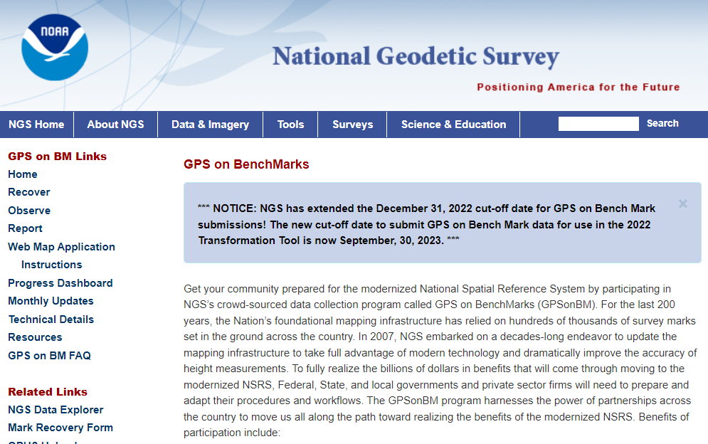
I’ve been highlighting NGS’s GPS on Bench Mark program that supports the 2022 Transformation Tool in my columns since 2018. NGS delayed the completion date for the new modernized NSRS until 2025, so they have extended the cut-off date for submitting GPS on Bench Mark data for use in the 2022 Transformation Tool until Sept. 30.
NGS GPS on BenchMarks Program (Image: NGS website)
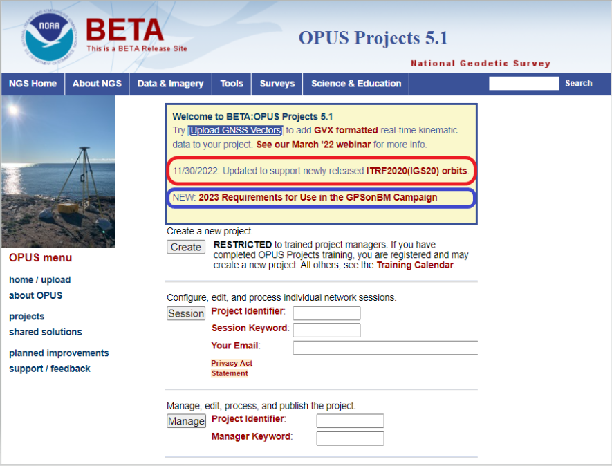
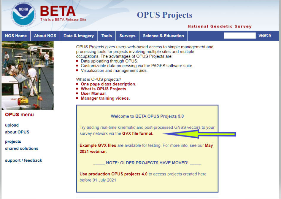
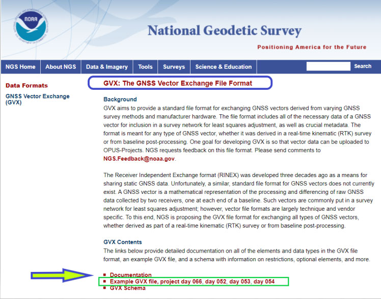
NGS has been developing tools that facilitate submitting data to the NGS GPS on BM campaign such as OPUS Share. The latest tool is the OPUS Project 5.1 routine that allows the use of RTN vectors. OPUS Projects 5.1 is a beta product, but NGS is now allowing users to use the routine to submit data for the GPS on BM campaign. My October 2021 column highlighted NGS’s Beta OPUS Projects 5.1.
The 2023 requirements for using OPUS Projects in the GPS on BM program (Image: NGS website)
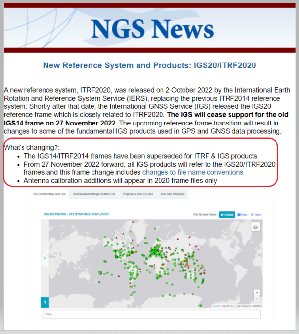
I’d like to note that OPUS has been updated to support the newly released ITRF2020 (IGS20) orbits. My October 2022column discussed the latest International Terrestrial Reference Frame of 2020 (ITRF2020) released by the International Earth Rotation and Reference System Service (IERS). A previous NGS news bulletin provided a statement about the new reference system and products.
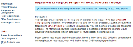
Clicking on the link titled “NEW: 2023 Requirements for Use in the GPSonBM Campaign” on the OPUS Projects 5.1 webpage provides the requirements for using OPUS Projects 5.1 and Real-Time Network (RTN) data to support the 2022 Transformation Tool; that is the 2023 GPS on BM campaign. There are five sections in the writeup: Introduction, Project Planning, Equipment and Configuration, Field Requirements and Office Requirements. The Introduction section states that the requirements are limited to the GPS on BM Campaign and will be replaced, or superseded, when NGS finishes its new GNSS surveying specifications.
Introduction Section from Requirement Write Up (Image: NGS website)
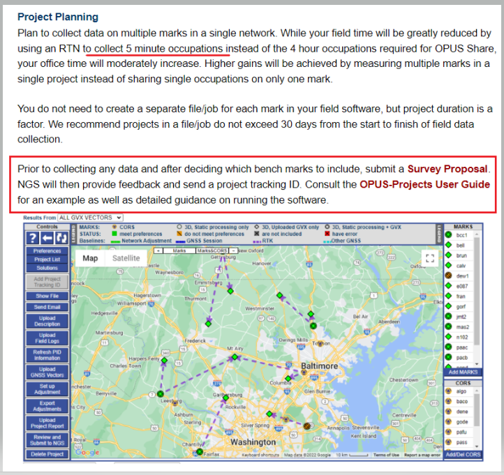
The project planning section of the announcement states that RTN vectors of 5-minute occupations can be used instead of the 4-hour occupations required for OPUS Share.
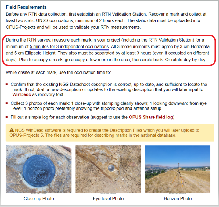
However, the Field Requirement section states that the mark must be occupied three different times.
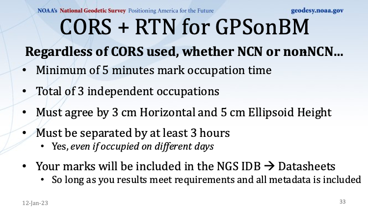
“During the RTN survey, measure each mark in your project (including the RTN Validation Station) for a minimum of 5 minutes for three independent occupations. All three measurements must agree by 3 cm horizontal and 5 cm ellipsoid height. They also must be separated by at least 3 hours (even if occupied on different days). Plan to occupy a mark, go occupy a few more in the area, then circle back. Or rotate day-by-day,” the section states.
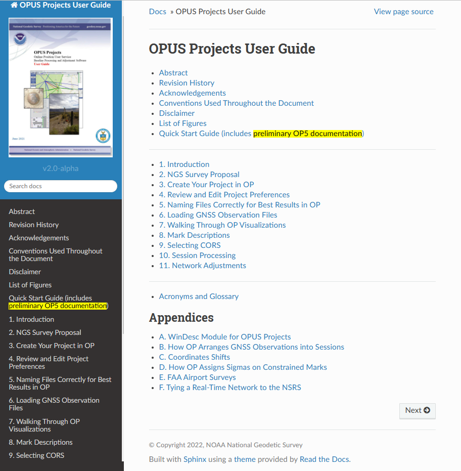
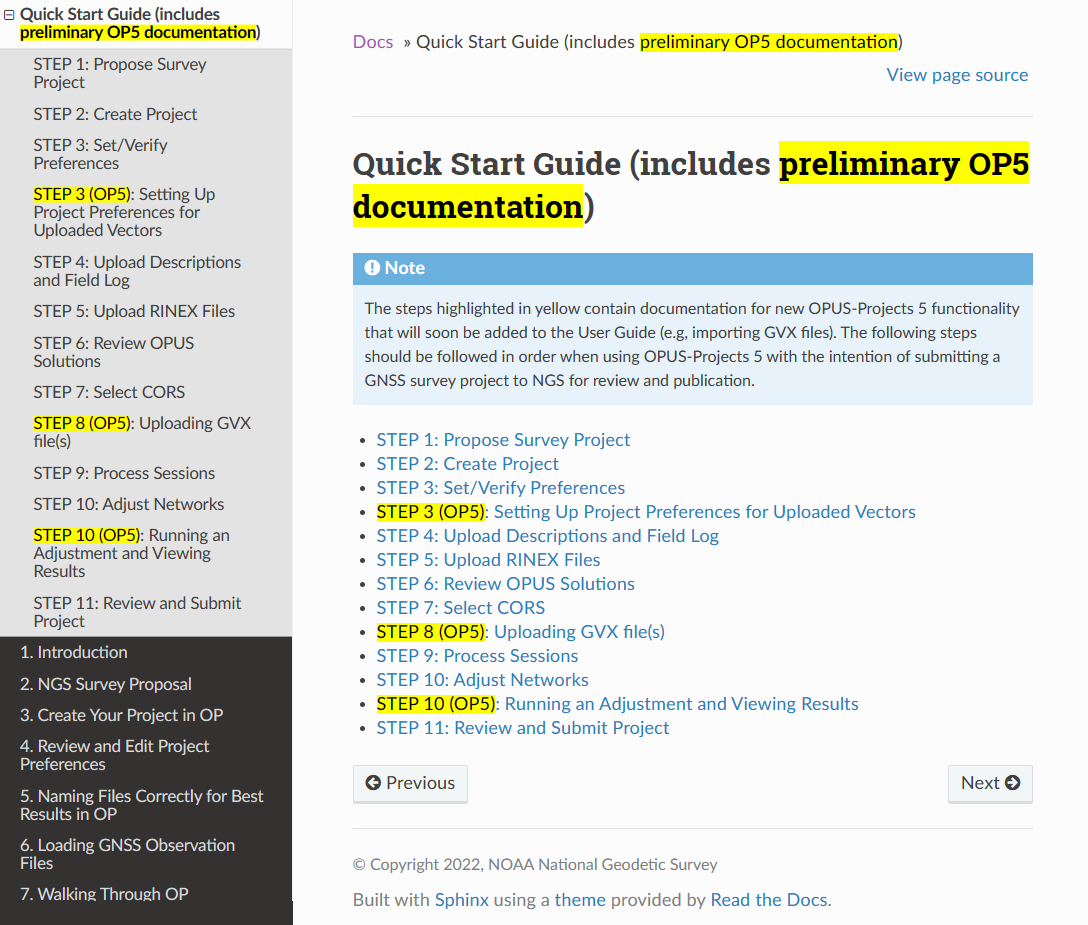
As stated in the section on office requirements for using OPUS-Projects 5 in the 2023 GPS on BM Campaign writeup,“The OPUS-Projects User Guide provides instructions on how to run the software and submit a project to NGS. The User Guide states to follow the steps in the order listed below, and it explains steps 1 – 7 and 9 – 11 in detail. For step 8 and when including GVX data in OPUS-Projects 5, refer to those portions of the User Guide’s Quick Start which are highlighted in yellow. NGS is working on fully updating the User Guide to include more details; for now, use the Quick Start Guide for assistance with GVX.”
OPUS Projects User Guide (Image: NGS website)Quick start guide. (Image: NGS website)
I recently used OPUS Projects to analyze some GNSS results using Harris-Galveston Subsidence District CORS and PAMS GNSS data. I want to emphasize that it may seem like a lot of work the first time you use the routine, but NGS makes it fairly simple to complete each task. The manual is very complete and does a good job of describing every step. The manual can be downloaded here. In my experience, the most time-consuming task is creating the descriptions. There are several items that must be correctly entered because the answer to some entries affect the answers to other entries. That said, NGS supports a description entry software called WinDesc that facilitates entering the appropriate information. The OPUS Projects User Guide provides an appendix that describes using the WinDesc module to enter description metadata.
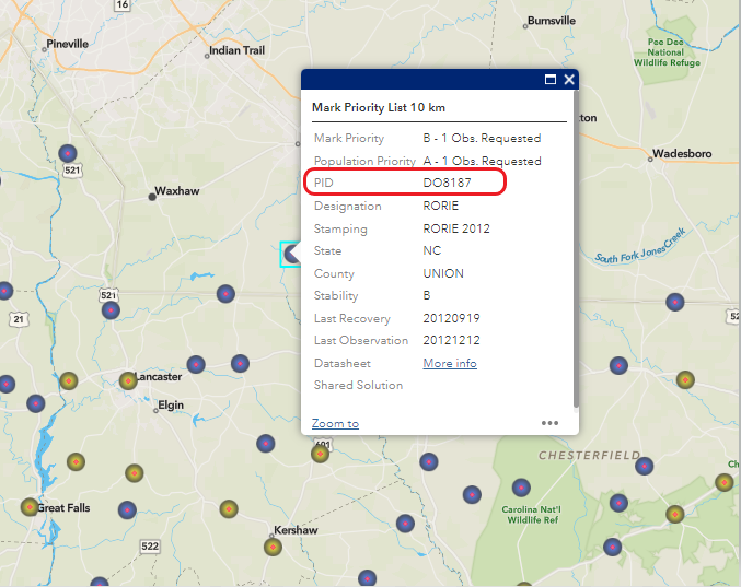
For marks that are in the NGS database, known as the NGS Integrated Data Base (NGSIDB), WinDesc will import information from NGSIDB, thereby decreasing the number of entries users need to address. In other words, if the mark has a PID then it should be in the NGSIDB. If you are occupying a mark that is part of NGS GPS on Bench Marks website then it probably has a PID and a description in NGSIDB.
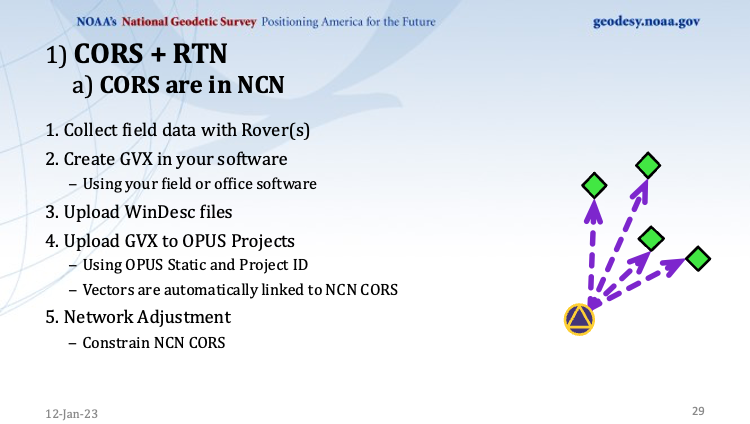
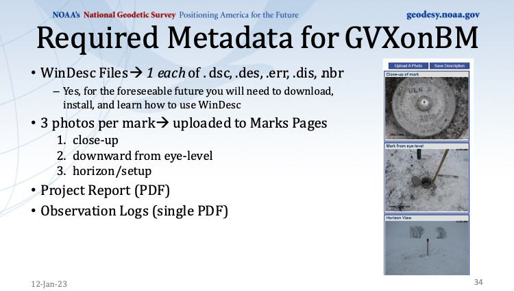
I’ve included three slides from the Jan. 12 webinar that summarize the basic requirements.
This slide is a depiction of how a CORS station must be connected to the RTN vectors. (Image: NGS website)This slide provides the occupation and precision requirements. (Image: NGS website)This slide provides a list of the required metadata for the project. (Image: NGS website)
As for the requirement of at least three independent RTN occupations on different times, in my opinion at least one occupation should be on a different day. My October 2021 column addressed a study that reported on using RTN solutions to estimate accurate horizontal and vertical coordinates.
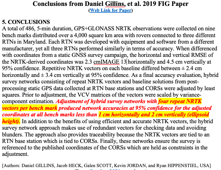
The report stated, “When differenced with coordinates from a static GNSS survey campaign, the horizontal and vertical RMSE of the NRTK-derived coordinates was 2.3 cm horizontally and 4.5 cm vertically at 95% confidence. Repetitive NRTK vectors on each baseline differed between ± 2.4 cm horizontally and ± 3.4 cm vertically at 95% confidence.”
The report also stated, “Adjustment of hybrid survey networks with four repeat NRTK vectors per bench mark produced network accuracies at 95% confidence for the adjusted coordinates at all bench marks less than 1 cm horizontally and 2 cm vertically (ellipsoid height).”
The requirements are limited to the GPS on BM Campaign and will be replaced, or superseded, when NGS finishes its new GNSS surveying specifications.
(Image: Screenshot of Accuracy of GNSS Observation from Tree Real-Time Networks in Maryland, USA)
The paper by Gillins, et. al was presented at the 2019 FIG Working Week held in Hanoi, Vietnam, on April 22–26, 2019. The International Federation of Surveyors (FIG), involves a wide range of professional fields within the international surveying community; this includes surveying, cadastre, valuation, mapping, geodesy, hydrography, and geospatial and provides an international forum for discussion and development to promote professional practice and standards. FIG meetings are held all over the world. I’d like to highlight that the 2023 FIG Working Week is going to be held in Orlando, Florida, on May 28 – June 1, 2023.
NGS will be presenting a full-day worth of content on NSRS Modernization during the FIG Working Week 2023. For the first time in more than 20 years, this annual FIG gathering will take place in the United States, hosted by the National Society of Professional Surveyors (NSPS).
I’ve participated in several FIG meetings. I’ve learned a lot from presentations as well as holding hallway meetings with experts from the international surveying and mapping community. All geospatial users should plan on attending this event. I have provided information about the FIG commissions in my August 2021 newsletter. I would encourage everyone to visit the FIG website and review the information about the 2023 FIG Working Week. The a list of the FIG Commissions can be found here. More information can be obtained on each commission by clicking on its title.
Future columns will highlight the FIG Working Week as the agenda is developed. I would encourage everyone to check NGS’s Website for updates on Beta products and new surveying specifications. Geospatial users should also subscribe to NGS’s News Services at the following here. Check out the NGS News Services site for what’s available.
Last year I was privileged to be part of a Blue-Ribbon Review Panel for an American Society of Civil Engineers (ASCE) surveying publication. The book is Surveying and Geomatics Engineering: Principles, Technologies, and Applications. I recently received my copy of the published book in the mail and decided to highlight some sections. While preparing this column, the chapters reminded me of how geodesy has expanded into so many different disciplines.
I first mentioned this in my July 2020 article for the “First Fix” column of GPS World, where I stated that the shortage of American trained geodesists poses a significant economic risk for the United States. In that column, I mentioned how geodetic science and technology now underpin many sciences, large areas of engineering (such as driverless vehicles and drones), navigation, precision agriculture, smart cities and location-based services. That is why I believe understanding geodesy is more critical today than ever. In January 2022, Mike Bevis, collaborating with others, prepared a white paper titled “The Geodesy Crisis,” documenting the concern about the lack of trained geodesists in the United States.
Image: Dana Caccamise II
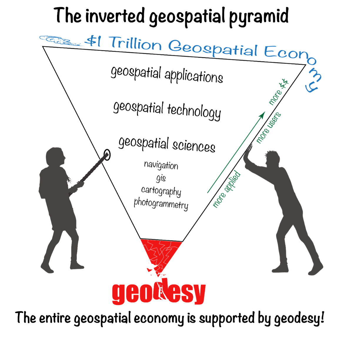
“The inverted geospatial pyramid” graphic depicts how the entire $1 trillion geospatial economy is supported and dependent on geodesy, and how it’s close to collapsing without an increase of support for geodesy. A lack of geodetic expertise in the United States presents a significant challenge, with future impacts on positioning, navigation, mapping and dependent geospatial technologies.
In my opinion, without investment in geodesy, the United States will not have the available skills and knowledge to develop new geodetic technologies and improve models to address challenges to society, such as
how the Earth’s surface is changing as sea level rises and the Earth’s glaciers and ice sheets change on timescales of months
how the tectonic plates are deforming and what physical processes control earthquakes, and
the ability to monitor the temporal changes in Earth’s water reservoirs by measuring changes in Earth’s gravitational field as it responds to the moving water mass and the deformation of the solid Earth caused by moving water.
These challenges need a well-maintained, stable terrestrial reference frame (TRF) with sub-1 mm/year vertical accuracy. Errors in TRF heights can propagate systematically into estimates of atmospheric water vapor, sea level, satellite orbits and other parameters. An accurate TRF can lead to important observations and discoveries because it enables revelations from coherent global motions. (My previous column described the latest International Reference Frame of 2020 [ITRF2020].)
Geodesy has been a significant part of my life for 50 years. I’ve seen a lot, and unless we address the Geodesy Crisis, the innovations in geodetic science of the past will not continue in the future. At least not in the United States.
The Geodesy Crisis paper was mentioned in the Fall 2022 ION Quarterly Newsletter by Everett Hinkley (see the box below). Hinkley noted, “The geospatial community relies on geodesists, though few in the community are fully aware of this connection nor understand the importance of geodesy to their work.” I encourage everyone to download the white paper and the ION Quarterly Newsletter to understand the importance of the need for more trained geodesists.
Excerpt from Everett Hinkley’s Article
“In January 2022, a white paper entitled America’s loss of capacity and international competitiveness in geodesy, the economic and military implications, and some modes of corrective action was released (Bevis et al.). This collaborative paper paints an alarming picture of the dwindling pool of trained geodesists within the United States. The report highlights America’s loss of capacity and international competitiveness in geodesy and states: ‘The U.S. is on the verge of being permanently eclipsed in geodesy and the downstream geospatial technologies. This decline in capability threatens our national security and poses major risks to an economy strongly tied to the geospatial revolution, on Earth and, eventually, in space.’ Though the word crisis correctly describes the dire predicament well, it didn’t occur overnight. Due to several converging trends, the geodesy crisis has been decades in the making. A national lack of geodetic expertise presents a significant challenge with downstream impacts on positioning, navigation, mapping, and dependent geospatial technologies. The Department of Defense, intelligence community, and federal civil agencies’ mapping entities rely on accurate and precise maps for a broad range of purposes, and reliable maps depend on an accurate geodetic underpinning. The geospatial community relies on geodesists, though few in the community are fully aware of this connection nor understand the importance of geodesy to their work.” (Reproduced with permission from ION.)
In my “First Fix” column, I mentioned that I attended The Ohio State University (OSU) to obtain my graduate degree in Geodetic Science in 1979. Therefore, I admitted that I am a little biased — once a geodesist, always a geodesist. That said, in OSU’s geodesy heyday (1960–1990s), many Americans trained were sent there by federal agencies: National Geospatial-Intelligence Agency (NGA), NOAA/National Geodetic Survey (NGS), USGS, Army, Navy and Air Force. During the 1970s, NGS sent two employees back to school every year. These agencies needed geodesists because they were undertaking significant projects, such as the NGS projects to readjust the U.S. national horizontal (NAD83) and vertical geodetic (NAVD88) networks. I was one of the employees NGS sent to OSU to be trained to support the NAD83 and NAVD88.
Today, the environment is different. U.S. federal agencies still need geodesists to develop enhanced and refined geodetic models and tools. However, major U.S. companies, such as Google and FedEx, the automobile industry, the construction industry (automated machine guidance), precision farming companies and mining companies also need more accurate geodetic models, tools and algorithms. Therefore, these companies also need trained geodesists to perform essential research on topics that address their geodetic requirements. As indicated in “the inverted geospatial pyramid” graphic, the entire $1 trillion geospatial economy is supported by geodesy.
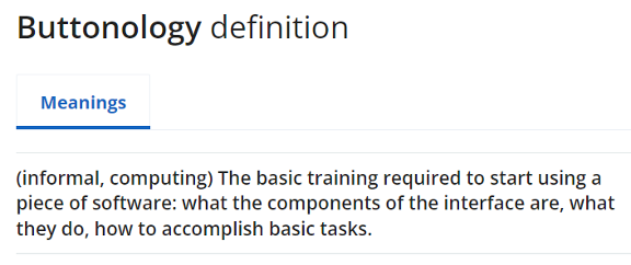
As implied in Hinkley’s article, geodesy has played a role in developing geospatial products but most users didn’t realize that it was their foundation. Since it’s been in the background, everyone assumes it will always be there. A participant at one of my workshops stated that “GPS has made geodesists out of all of us.” In my opinion, the advancements in GNSS equipment and processing software provided some users with a “false sense of knowledge or security” that they understood what was happening within the “black box.” One of my colleagues at NGS said that the new equipment and software programs were creating a field force of “buttonologists.”
These statements concerned me at the time and concern me today. With the last generation of trained geodesists either retired or getting ready to retire, we are at a critical stage of not being able to meet the geospatial needs of the future. As indicated in the white paper, there are significant challenges in rebuilding programs that support the training of geodesists.
Hinkley’s article summarized several action items that could help improve the lack of trained geodesists in the United States. I’ve provided his list in the box below. I’ve highlighted several items the surveying and mapping community can help achieve.
So how do we build and educate the next generation of geodesists?
Make the White House and Congress aware of this crisis, particularly its national security implications; seek direct support in the federal budget to correct this issue. It has become clear that, without engagement at the highest echelons of the U.S. government, averting this current crisis and its eventual outcome is unlikely.
Teach rigorous math in our public schools; follow the scholastic math approach used in many Asian and European countries.
Encourage creative thinking!
Actively market geodesy in high schools as a rewarding career for the math stars before college entry.
Build back, support and sponsor geodesy programs at select universities. This support needs to be strategic, with backing from the highest levels of the U.S. government.
Break our cultural trend of reactions to crises and seize the opportunity to be proactive and prevent the foreseen consequences of this crisis.
Encourage U.S. government support in the form of grants, professional development of staff, and research collaborations/affiliations. There are early efforts underway to bring new talent into the pipeline:
the National Geospatial-Intelligence Agency (NGA) is forming an emerging scientist consortium (ESCON) with partnerships that exist with Ohio State, UT-Austin, and other industry/academic/government partners
a pilot Ph.D. geodesy educational program with three NGA and one NGS employee is in place; the NGA expects to continue growing this program.
the NGA’s new western headquarters in St. Louis will bring 350 companies and organizations into the regional GEOINT ecosystem.
If we answer this call to action collectively, there is hope that a new cadre of U.S. geodesists can be cultivated before it’s too late to recover.
(Reproduced with permission from ION.)
With all that said about the need for more geodesists, one thing that this ASCE publication may do is make some readers realize how much they don’t know about the roots of the technology that they’re using to create geospatial products and services. This knowledge gap is not just correctly using GNSS and other geospatial technology to perform a survey, but also integrating various instruments to create an accurate mapping system, such as mobile mapping and terrestrial laser systems. My intent is not to criticize the expertise or knowledge of anyone, and I only mean to point out that in today’s use of computers and programs, many technical concepts are hidden in “black boxes.” I learned many things about some topics by reviewing this book.
The book is 556 pages and has 15 chapters. As part of my responsibilities as a Blue-Ribbon Panel member, I read every word in the book, and not many people will read the entire book. Still, I would encourage surveyors, engineers, geodesists, photogrammetrists and GIS and remote-sensing practitioners to obtain a copy of the book for reference and to understand the limitations of geospatial technology.
Now to the book’s content. I want to highlight that the forward is written by Juliana Blackwell, director of the National Geodetic Survey (NGS). She states that “A common thread running through the manual is the importance of the National Spatial Reference System (NSRS) to modern geospatial applications.”
Most of my columns highlight something relevant to the NSRS. That’s because the NSRS is the foundation layer for United States federal geospatial products, and geodesy provides the foundation for all geospatial products and services as indicated in the “The inverted geospatial pyramid” figure.
I would also like to highlight a statement by Gene Roe in the preface. He states, “Because entire books could be devoted to each of these topics, this manual only provides a summary, and it points the readers to important references where they can find more details. The manual is meant to provide a comprehensive but general overview to help support education and inform practicing engineers on the important role of the surveying engineer. It is too important for this not to occur.”
I agree with Roe’s statement that the book is important for surveying engineers. Still, I would add that this book is important to anyone working with GNSS and other geospatial data, especially geodesists, surveyors and GIS practitioners.
This publication is edited by three individuals that are licensed surveyors; two of them are geodesists who work for NGS. These individuals have performed a fantastic job of ensuring that all chapters have been reviewed for correctness and that the information provided is current and essential for users of geospatial data.
Readers can download copies of the book and specific chapters here. You can buy it as an e-book or in print. The “Abstract” box summarizes the book from the ASCE Library website.
Abstract
Sponsored by the Surveying Committee of the Surveying and Geomatics Division of the Utility Engineering and Surveying Institute of ASCE and the National Geodetic Survey of the US National Oceanic and Atmospheric Administration
Surveying and Geomatics Engineering: Principles, Technologies, and Applications, MOP 152, is a comprehensive yet general overview to help support education and inform practicing engineers on the important role of the surveying engineer. It provides a much-needed update on the modern practice of surveying and geomatics engineering.
Topics include:
• geodesy
• coordinate systems and transformations
• least squares adjustments and error propagation
• modern surveying and remote sensing technology
• analysis and establishment of control
• geographic and building information systems
• construction surveying, and
• best practices.
MOP 152 can be used as a summary and a reference for practicing engineers, surveying and otherwise, to help provide a solid understanding of the state of the surveying and geomatics engineering field.
Below is a list of the chapters and their authors. This column cannot highlight everything important in this book, but I will select a few items to which I believe users of geospatial data should pay attention.
Chapter Titles
Chapter Number
Chapter Title
Author(s)
Forward
Juliana P. Blackwell
Preface
Gene V. Roe
Acknowledgments
Daniel T. Gillins
1
Engineering Surveying Within ASCE
Gene V. Roe
2
Geodesy and Geodetic Computations
Earl F. Burkholder
3
Map Projections and Local Coordinates Systems
Michael L. Dennis
4
Local, Regional, and Global Coordinates Transformations
Michael L. Dennis
5
Analysis and Adjustment of Observational Errors
Charles D. Ghilani
6
Satellite-Based Surveying Technology
Jan Van Sickle
7
Leveling and Total Stations
N.W.J. Hazelton
8
Terrestrial Laser Scanning
Michael J. Olsen
9
Mobile Terrestrial Laser Scanning and Mapping
Michael j. Olsen, Jaehoon Jung, Erzhuo Che, Chris Parrish
10
Aerial Surveying Technology
Michael J. Starek, Benjamin E. Wilkinson
11
Survey Control
Daniel T. Gillins
12
Construction Surveys
Marlee A. Walton
13
Survey Records
Andrew C. Kellie
14
Information Systems in Civil Engineering
Yelda Turkan, Dimitrios Bolkas, Jaehoon Jung, Matthew S. O’banion, Michael Bunn
15
Professional Services and Design Professionals Agreements
David E. Woolley, Lisa D. Herzog
As a geodesist, I usually focus on topics relevant to geodetic science. This book has a lot of topics that use geodesy concepts to create an engineering product or service. For example, chapter 2, “Geodesy and Geodetic Computation” by Earl Burkholder, provides a good summary of geodetic concepts that anyone using or generating geospatial products should know and understand. It gives basic equations without lengthy derivations of how they were developed.
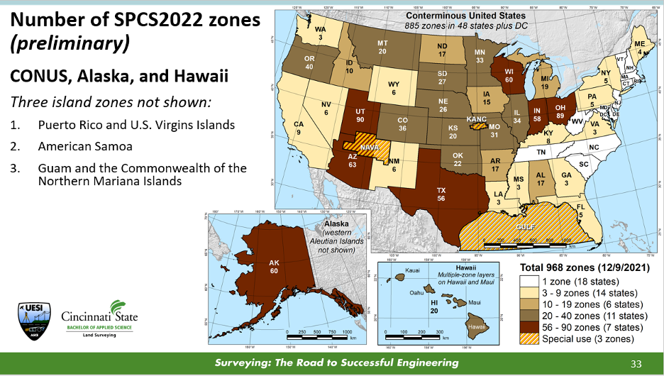
In my opinion, chapter 3, “Map Projections and Local Coordinates Systems” by Michael Dennis, does the best job of explaining the concepts of map projections that are relevant to the surveying and mapping community. Many GIS practitioners use map projections in their software but don’t have a working knowledge of what’s happening to their original data. This chapter describes the current United States State Plane Coordinate System of 1983 (SPCS83) and the future State Plane Coordinate System of 2022 (SPCS2022) that is scheduled to be adopted in 2025. Dennis uses figures and diagrams to describe map projections, angular and linear distortion, and methods for reducing map projection distortion to make it easier for readers to understand the concepts. One section of interest to many surveyors after SPCS2022 is adopted is the Low-Distortion Projection (LDP) Coordinate Systems section. This is useful because, in SPCS2022, many states have designed LDP systems for their state’s SPCS2022. The box below provides a diagram with the number of zones for each state.
Image: NGS Presentations Webpage “Grids for the Future: A New Approach for Designing State Plane Coordinate System Zones” by Michael Dennis.
One purpose of an LDP is to reduce linear distortion; it is not a new concept. Many surveyors have performed a simplified form of it for decades. It’s known by many as a “modified” or “scaled” State Plane. The American Congress on Surveying and Mapping (ACSM) taught a workshop for decades describing how to compute a “modified” State Plane Coordinate. I was an instructor of this class in the 1980s and 1990s. “Modified” State Plane Coordinates had several issues, but they worked reasonably well in small areal extents. Today, with the advancements in computers and computer software, there are better ways to accomplish an LDP. Dennis’ section does a great job explaining the new SPCS2022 and the design of LDPs in the SPCS2022. The use-case examples provide a simplified description of understanding the linear distortion behavior in an area.
Chapter 4, “Local, Regional, and Global Coordinate Transformation” by Michael Dennis, is one that every surveyor and GIS practitioner should read. Dennis highlighted the differences between “equation-based” transformations and “grid-based” transformations, as well as combined equation-based transformations with grid-based transformations. Understanding the information provided in chapter 4 will be important when NGS replaces the NAD 83 (2011) and NAVD 88 datums with the new, modernized NSRS in 2025. NGS will provide models and tools for users to perform coordinate transformations, but hopefully, some users will want to understand what’s happening behind the scenes.
Chapters 8 and 9 discuss laser scanning systems. In chapter 8, “Terrestrial Laser Scanning,” the “Data Quality Considerations” section highlights common artifacts or limitations encountered with terrestrial lidar system data. The authors provide many examples of these artifacts, making the concept easy to understand. At the end of this chapter, there are 14 pages of references that will be very helpful to users involved with terrestrial laser scanning systems.
Chapter 9, “Mobile Terrestrial Laser Scanning and Mapping,” is very informative, especially the section on georeferencing. This section is not just the description of properly using GNSS to perform a survey, but also the integration of various instruments to create an accurate mobile mapping system. I like how the authors discussed the error sources in georeferencing the system, listed the source, and provided an explanation of the error.
Anyone performing a GNSS survey project that meets NGS’s requirements needs to read chapter 11. I like the section describing how users should evaluate CORSs before using them as control. Evaluating CORS is something all users should do before using any CORS in their project, because not all CORS are created equal. See the excerpt from chapter 11 below for the recommended steps from the author.
Excerpt from Chapter 11 – Steps for Evaluation of CORS
The author recommends the following steps:
1. Choose stations that are within 100-300 km of a project site. It is well known that errors in GNSS baseline processing are directly correlated with baseline length (Chapter 6). Tropospheric delay is reduced when baselines are shorter and atmospheric conditions at each end of the line are similar. In addition, mutual satellite visibility at each end of the line for differencing diminishes as baselines grow longer. That said, errors in GNSS processing are more occupation time-dependent than baseline length-dependent (Eckl et al. 2001). Therefore, for short GNSS sessions (i.e., < 2 hours), choose CORS within approximately 100 km as control; for moderate GNSS sessions (i.e., 2 to 8 h), choose CORS within approximately 300 km. Note that even longer baselines can be successfully processed when GNSS sessions are very long in duration (e.g., up to 2,000 km for 24 h sessions).
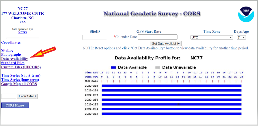
2. Determine if GNSS data are available at a given CORS during the time of your survey. Of course, if data are unavailable, then the station simply cannot be used as control. NGS provides a tool known as “User Friendly CORS (UFCORS)” for entering a date and time range to view available data at a given station (NGS 2021c). This tool can also be used to download the raw GNSS data for processing and adding a station to the survey network.
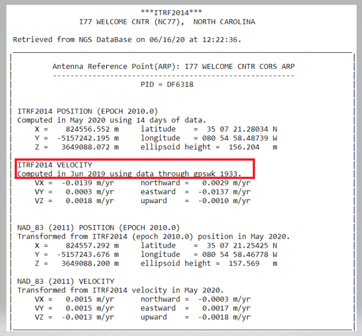
3. As discussed previously and when possible, choose a CORS with computed velocities rather than modeled velocities from HTDP. NGS provides tables of official coordinates with “computed” versus “htdp” coordinates and velocities on the website for CORS.
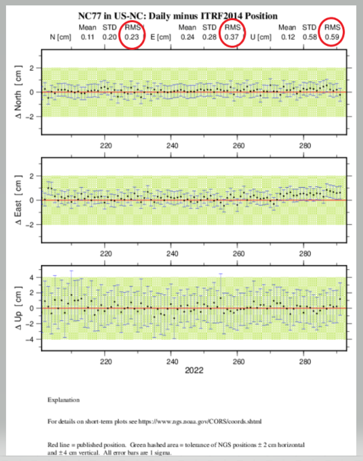
4. Review the aforementioned short-term time-series plot for the station, ideally at the time of the project. Stations with large spikes, data gaps, bias from the published “red” line, or large standard deviations should be avoided. A good rule-of-thumb is for the RMS in the short-term time-series plot (Figure 11-2) to be less than 1.0 cm in north and east and 2.0 cm in the up direction in a local geodetic horizon frame at the station.
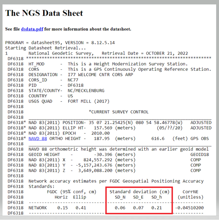
5. Examine the formal uncertainties for the official coordinates of the CORS. Standard deviations in north, east, and up are provided on the station’s datasheet, accessible from the webpage for the CORS (more on datasheets are discussed in the following under Passive Control). Stations with unusually large standard deviations (> 3 cm) should be avoided. Note that standard deviations are not available for CORSs with modeled velocities.
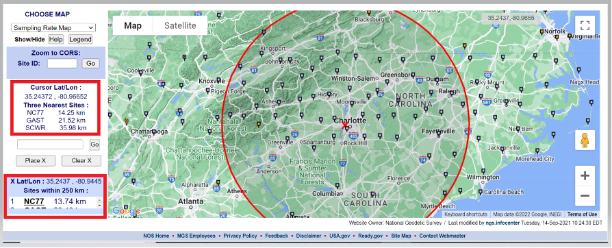
I believe that the evaluation of NOAA CORS is critical, so I’ve described Dan Gillins’ “Steps for Evaluation of CORS” below. First, users can access the NOAA CORS using the NGS CORS Map utility. After the map appears, users can move the cursor over the center of the project area, where it provides the location of the cursor and the three closest CORS. Users can click on a CORS icon and get coordinates and other information about the CORS. Also, they can place an X on the map, and the utility will draw a 250-km circle around the point. The box in the lower left-hand side of the map provides a list of the sites within 250 km of the marked location.
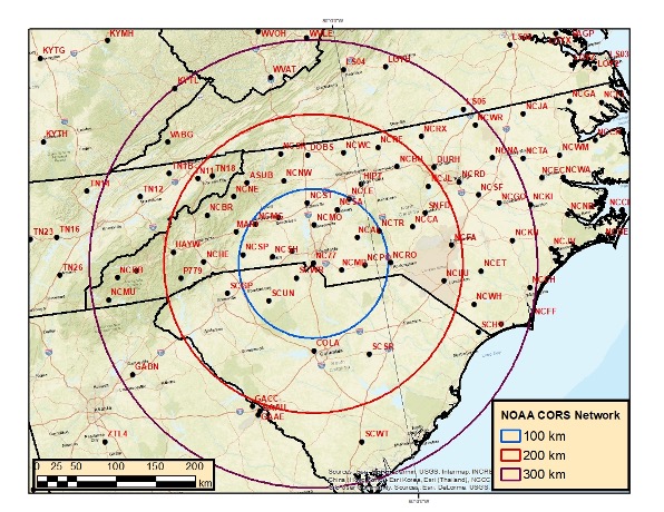
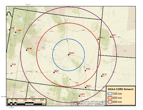
Users can download the NOAA CORS coordinates and velocities (computed and modeled). I downloaded the files and plotted three circles (with radii of 100, 200, and 300 km) around CORS NC77 in Charlotte, North Carolina. I only plotted CORS that are operational and have computed velocities. North Carolina has a lot of CORS to select from. In contrast, I’ve plotted three circles (also with radii of 100, 200 and 300 km) around CORS WYRF in Casper, Wyoming.
Buffer Zones around Charlotte, NC
Image: Dave Zilkoski
The plot depicting the buffer zones around Casper indicates that there are no CORS within the 100-km circle and only a few between 100 and 200 km.
Buffer Zones around Casper
Image: Dave Zilkoski
The data availability of the CORS site can be obtained by clicking on the CORS icon, selecting “Get Site Information,” and then selecting “Data Availability.”
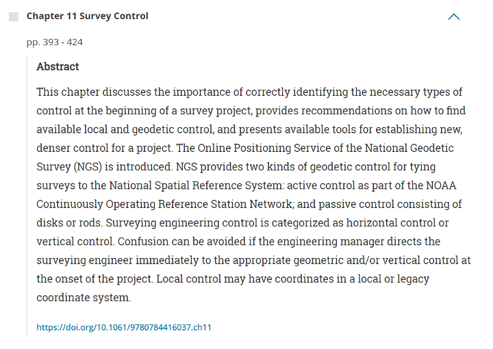
There are too many chapters to describe each one, but I encourage users to check each chapter’s abstract on the ASCE website and decide which ones would be the most beneficial to them (see the box titled “Abstract for Chapter 11 Survey Control”). The manual provides numerous references and can serve as a helpful resource for finding further details on the fields of geodesy and surveying.
A goal of mine is for some readers of this column to obtain enough knowledge to “whet their appetite” and encourage them to pursue an education in geodesy and surveying. Others who are influential in federal government programs and those responsible for geospatial research for industries will recognize the need for more trained geodesists in the United States and help by doing the following:
actively market geodesy in high schools as a rewarding career for the math stars before college entry
build back, support, and sponsor geodesy programs at select universities; this support needs to be strategic with backing from the highest levels of the U.S. government
encourage U.S. government support in the form of grants, professional development of staff, and research collaborations/affiliations.
Technology changes the rules of the game, and surveying may be more in its crosshairs than the profession will admit
Maps have existed for centuries. The lines on maps indicating the boundaries of political and administrative units — cities, counties, states, and countries — are graphic representations of the limits of those entities. These lines don’t, however, typically exist in real life. There isn’t a large line between the United States and Canada stretching from the Pacific Ocean, through the Great Lakes, and onto the Atlantic Ocean.
The same goes for latitude and longitude lines on maps and globes. The public generally accepts the various delineations on maps as being somewhat accurate with an unwritten level of trust in those who have produced these maps.
Definition
trust: assured reliance on the character, ability, strength, or truth of someone or something.
Here are the guidelines surveyors use for determining surveys.
lines physically verified in the field and proven from evidence
monuments and/or boundaries set and called for within legal descriptions
natural monuments
artificial monuments
adjoiners (to determine junior/senior rights)
courses
bearings, then distances (metes and bounds states)
distances, then bearings (public land survey states)
recitation of area
controlling description
evidentiary description
coordinates: local and/or geodetic
Surveyors rely on physical monuments, title documents and evidence of occupation to assist with the establishment of not just major dividing lines, but all lines of property, public or private. Finding, setting and honoring physical monuments has been a significant character trait of the surveyor for as long as maps have existed.
Monuments are placed to determine the endpoints of these lines as depicted on maps or plats, but what happens when technology introduces new ways to re-establish these lines? What will happen to our monuments when technology — more specifically those who utilize them — deems them obsolete?
The guidelines above are known as “priority of calls” or “rules of construction” by the surveying community. These items have provided the instructions for surveyors to follow in retracement of lines for many years. However, like nearly everything else in our modern world, technology has a hand in modernizing even this time-honored “surveyor’s code of retracement.”
Who would have guessed that the rotary phone dial would give way to touch-tone buttons, that the system would jump from landlines to cellular and satellite signals to remote handsets, then progress to receivers evolving away from physical buttons to touchscreens?
Technology changes the rules of the game, and surveying may be more in its crosshairs than the profession will admit.
Here come the numbers
Note that the last entry in the above guidelines for survey retracement is “coordinates.” In accordance with most accepted lists, coordinates can be local or geodetic. These coordinate values are generated by surveyors, geodesists and public agencies; they can be found on plats, and in records and websites kept by government agencies.
Now that we are more than two decades into the 21st century, it would be safe to say that most of the surveying profession uses an established geodetic coordinate system. The use of GNSS receivers is widely accepted as normal practice by many surveyors because these systems are much more user friendly than in years past. Additional constellations have added to the availability and accuracy of GNSS positional values, so utilizing state plane coordinates has become the norm.
We are now surrounded by something that has an incredible impact on our profession and the world around us. We are placing trust in a georeferenced coordinate system that cannot be identified by any of our senses, like we can with a physical monument.
A coordinate cannot be seen, touched, tasted, heard or smelled.
We are placing our full trust in a reliable position on Earth as determined by our GNSS receiver working within a published coordinate system. Because of these advancements in technology, a new generation of geospatialists is insisting we should revise the way we survey, because technology provides much higher precision and accuracy.
Just like lines on a map or plat, coordinates only exist as a calculation of a position on the face of Earth. So why is there animosity in trusting coordinates over the more traditional items on the list of retracement guidelines? It may have to do with the fact that the ground we are surveying is not in the same place it was a short time ago. Depending on where you live, it may have moved more than you think. For more information on the shifting ground we live on, let us dig into some research about our continents.
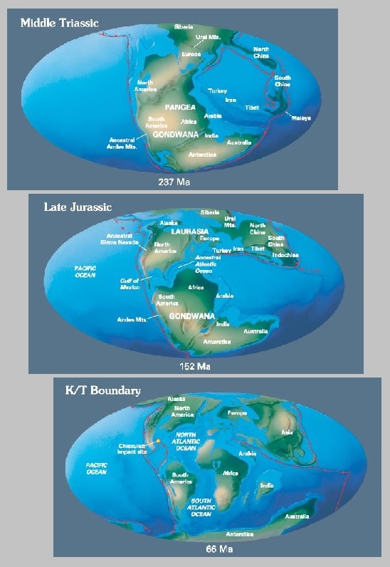
From about 300-200 million years ago (late Paleozoic Era until the very late Triassic), the continent we now know as North America was continuous with Africa, South America and Europe. They all existed as a single continent called Pangea. Pangea first began to be torn apart when a three-pronged fissure grew between Africa, South America and North America. Rifting began as magma welled up through the weakness in the crust, creating a volcanic rift zone. Volcanic eruptions spewed ash and volcanic debris across the landscape as these severed continent-sized fragments of Pangea diverged. The gash between the spreading continents gradually grew to form a new ocean basin, the Atlantic. The rift zone known as the mid-Atlantic ridge continued to provide the raw volcanic materials for the expanding ocean basin.
Meanwhile, North America was slowly pushed westward away from the rift zone. The thick continental crust that made up the new east coast collapsed into a series of down-dropped fault blocks that roughly parallel today’s coastline. At first, the hot, faulted edge of the continent was high and buoyant relative to the new ocean basin. As the edge of North America moved away from the hot rift zone, it began to cool and subside beneath the new Atlantic Ocean. This once-active divergent plate boundary became the passive, trailing edge of westward moving North America. In plate tectonic terms, the Atlantic Plain is known as a classic example of a passive continental margin.
Today, the Mesozoic and Cenozoic sedimentary rock layers that lie beneath much of the coastal plain and fringing continental shelf remain nearly horizontal.
Image: USGS
In geologic terms, a plate is a large, rigid slab of solid rock. The word tectonics comes from the Greek root “to build.” Putting these two words together, we get the term plate tectonics, which refers to how the Earth’s surface is built of plates.
The theory of plate tectonics states that the Earth’s outermost layer is fragmented into a dozen or more large and small plates that are moving relative to one another as they ride atop hotter, more mobile material. Before the advent of plate tectonics, however, some people already believed that the present-day continents were the fragmented pieces of pre-existing larger landmasses (“supercontinents”).
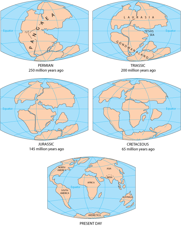
The diagrams below show the break-up of the supercontinent Pangaea (meaning “all lands” in Greek), which figured prominently in the theory of continental drift — the forerunner to the theory of plate tectonics.
Image: USGS
Continental drift, plate tectonics and prime meridians
Historians and other scientists have theorized about Pangea for centuries. Common soil types, fossils, and other evidence found on different continents help to solidify the concept of Pangea. Items discovered on the west coast of Africa have many similarities with those found on eastern South America. The physical evidence is quite convincing that an earlier supercontinent existed millions of years ago.
Now, let’s apply a fixed measurement system with lines upon Earth that defines latitude and longitude. In the past, geodesists, geographers and mathematicians established various “prime meridians” around the world to serve as a basis for maps. Locations and cities used included Amsterdam, Antwerp, the Bering Strait, Bern, Brussels, Copenhagen, Florence, Giza, Jerusalem, Kyoto, Lisbon, Madrid, Naples, Oslo, Paris, Philadelphia, Pisa, Rio de Janeiro, Rome, Stockholm, Warsaw and Washington, D.C. (in four different places!), just to name a few.
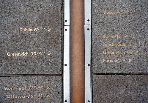
Thankfully, scientists gathered in the 19th century to agree upon a singular “initial meridian” that would pass through Greenwich, England, and was based upon several centuries of astronomical observations at the nearby Royal Observatory.
For approximately 100 years, mapmakers (and geodesists) used the new Prime Meridian at Greenwich as the beginning baseline for longitude determination around the world. After all, it was based upon years of astronomical observations and solved the age-old problem of where longitude starts. (Latitude was a much easier calculation for astronomers and geodesists, but that story is for another day.)
The late 20th century and the fourth industrial revolution
Technology, once again, provides us with conflicting results. While most technological advancements are game-changing improvements to mankind, they also tend to shake up information and standards that have existed for many generations. Like the previously discussed advancements in telephones, technology makes us change the way we look at things and how we go about our lives.
Mapping has become a central part of our everyday lives. Georeferenced positions for literally everything is now a standard characteristic of many functions within our environment, especially in our surveying world. Most of these improvements are due to GPS, which was originally developed for the U.S. military to guide and assist with positional location of our defense systems in relation to our enemies. We use this same precise technology to establish positional locations for boundary points, infrastructure and topographic information.
Image: Tim Burch
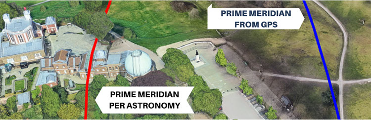
We have also used GPS to learn much about our tectonic plates and varying movement of the continents.The first thing we learned is that the Prime Meridian established in 1884 does not fall in the same place as our 0° latitude designation as determined by GPS/GNSS calculations.
This finding, however, is not the telling item within our adaptation of GPS data; it came when various agencies established the continuously operating reference system (CORS), composed of static GPS base stations. CORS stations, while used to help establish new survey positions in relation to a known reference location, also measure a continuous drift of latitude and longitude positions over time.
The National Geodetic Survey (NGS) is in the process of finalizing a new reference framework for establishing coordinate values that utilize time as a core component. Future implementation of the new National Spatial Reference System (NSRS) will require the additional attribute of time within the metadata of any new values.
So how does this affect surveying and the monuments we surveyors hold on such a high pedestal? The answer varies depending on who one asks. Most surveyors will continue to hold the “priority of calls” as listed above. Several practitioners, however, want to move coordinates higher up the list because of technology, and the ability to retrace a published point because of the increase in technology and the higher accuracy and precision of today’s GNSS.
This is possible if the user of the technology follows the procedures as established by NGS with metadata and accurate timing, but there are still several variables in the setting and retracing methodologies. When was the last time the equipment was calibrated? Was adequate research performed to minimize environmental errors? Was there any interference due to solar storms or multipath? There are many potential issues a surveyor can face, but few are checking all the boxes when performing highly accurate and precise positional measurements.
Technology has brought surveying into the 21st century with GPS/GNSS and ever-increasing accuracy and precision. It should also be the profession’s goal that the technology does not override what the general public can see. They can see monuments, fence lines, buildings and other improvements, but they cannot see coordinates, which remain invisible to the naked eye. Technology may change that in the future, too, but until that time, we must rely on what we can see.
My previous column highlighted that orthometric heights in NAPGD2022 will be defined through ellipsoid heights and a geoid model, such as GEOID2022. Therefore, changes in the geoid model will be very important to users estimating orthometric heights using GNSS. I briefly described the geophysical reasons for changes in the geoid that affect the orthometric height of a mark.
For the past four years, I have discussed in my columns the tasks associated with the new, modernized 2022 reference frames. It’s now the middle of 2022, so where are the new reference frames? Well, on June 9, Dru Smith, NSRS modernization manager for the National Geodetic Survey (NGS), provided an update on the status of the modernization in a webinar. The Powerpoint slides and video of the presentation can be downloaded from the NGS website under the following title: It’s 2022…Are You Done Yet? I will highlight some of the items from the webinar, but I encourage everyone to download the video and listen to the webinar.
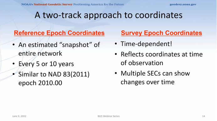
First, Smith mentioned that NGS will be providing new types of coordinates. The NGS denotes this as a two-track approach to coordinates: Reference Epoch Coordinates (REC) and Survey Epoch Coordinates (SEC). See the box below.
New types of coordinates (Image: NGS June 6 webinar)
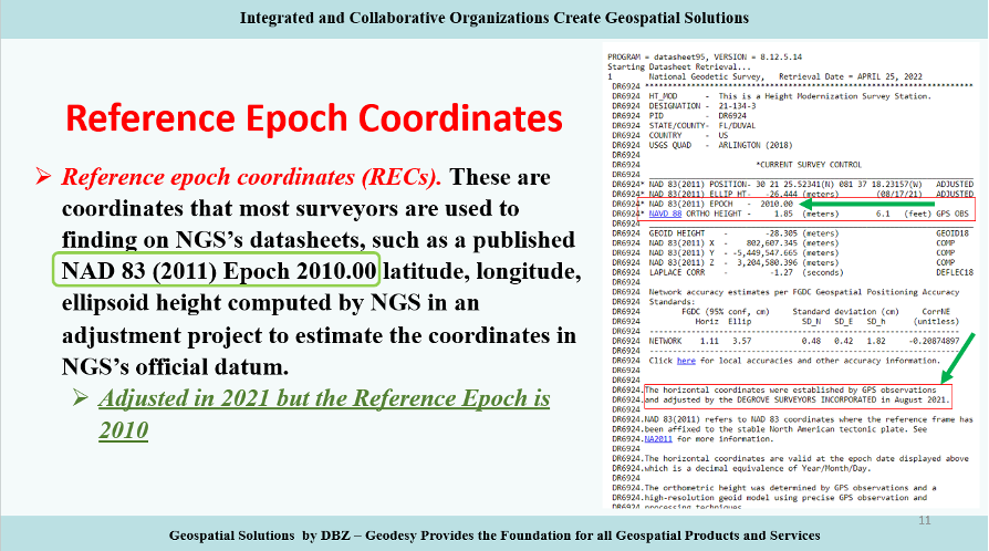
Reference Epochs Coordinates (REC) are defined in NGS Blueprint for the Modernized NSRS, Part 3 as coordinates computed by NGS in an adjustment project to estimate the coordinates at one of the official reference epochs that NGS will define in 2025. RECs are similar to coordinates computed by NGS in a nationwide adjustment project such as the National Adjustment of 2011 (see the box below).
NAD 83 (2011) epoch 2010.00 coordinates (Image: NGS)
NGS has not determined what data will be included in the first iteration of RECs. For the 2020.00 project, the current cutoff date for incorporating data is Dec. 31. Users can submit the data to NGS via OPUS projects and the OPUS-Share tool. To increase the submission of GNSS observations on marks, NGS has developed a beta OPUS-Projects 5.0 webtool that will allow real-time kinematic and real time network (RTK/RTN) observations to be submitted.
As previously mentioned, at this time, the NGS has not determined the cutoff for the earliest data to be included in the determination of the 2020.00 RECs. The agency will be conducting experiments to determine the appropriate cutoff date. These coordinates will require an intra-frame velocity model (IFVM) to generate the RECs at the specific reference epoch.
As of February 2021, based on NGS’ Blueprint for the Modernized NSRS, Part 3, version February 2021, the following is the agency’s policy with regard to RECs:
For a given mark and a given reference epoch, the REC will never be changed–except to correct a blunder.
This does not prevent NGS from adding new RECs
on points with new data that have not yet had an REC computed
for marks that do not have an REC in the most recently passed reference epoch, a new REC can be computed and added to the NSRS.
Survey epoch coordinates (SECs) are defined as coordinates computed by NGS at a specific survey epoch. Users will submit their data and its metadata to NGS, and NGS will then check, adjust and define the coordinates at one “survey epoch.” These coordinates will be “part of the NSRS,” Smith said. NGS is computing coordinates in this manner to provide the best estimate of the coordinates at any mark at a specific moment in time, which is very important in areas influenced by crustal movement.
So, how will NGS process and generate these SECs?
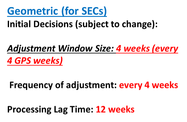
Survey epoch coordinates (SECs) are designed to provide time-dependent geodetic coordinates. Therefore, NGS has to choose some time span in which all observations will be processed together to yield a single SEC of a mark. NGS denotes this time span as a “geometric adjustment window.” NGS wants the adjustment window to be short enough so that movement of a mark did not occur between repeat observations (or was small enough to be ignored) and long enough for users to efficiently and effectively collect redundant observations for submission to NGS (see the box below).
One or more GNSS occupation(s) over a single mark will be processed into one survey epoch coordinate when all occupations take place within one geometric adjustment window.
If a user submits two occupations on one mark, but they happen to fall in two consecutive geometric adjustment windows, NGS will use them to create two distinct survey epoch coordinates. Each SEC will be based on one occupation.
Future columns will provide more explanation about this concept of a geometric adjustment window and how NGS will process the data to generate survey epoch coordinates.
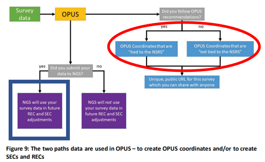
NGS is developing models and tools for users to submit data to NGS to compute coordinates — including OPUS coordinates, reference epoch coordinates and survey epoch coordinates. Figure 9 from Blueprint for the Modernized NSRS, Part 3, version February 2021, is a schematic that shows the flexibility NGS is building into an OPUS-type webtool. Basically, if users follow NGS guidelines and rules, and submit their data to NGS, then NGS will compute and publish REC and SEC coordinates (see the blue outline in the box below). If users only want to compute OPUS coordinates, then they can use NGS’s webtool without submitting the data to NGS (see the red outline in the box below).
Building flexibility into OPUS (Image: NGS)
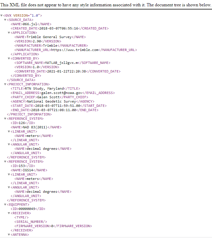
Dru Smith’s June 9 update on the status of the modernization provided a mockup of how users will be able to retrieve data using their web browsers — a prototype is being developed. The data will also be available in downloadable form such as an XML file for users to input the data and metadata into their programs or databases. I recently discussed some of this material at seminars I presented at the Florida Surveyors and Mapping Society’s 67th annual conference held in Palm Beach Gardens. The participants were very interested in the prototype, but really wanted to learn more about the format and process of the downloadable XML files. I’m sure future NGS webinars will address this topic. I emphasized to the group that they should watch the entire presentation and provide feedback to NGS. As mentioned above, Powerpoint slides and video can be downloaded from the NGS webinar website.
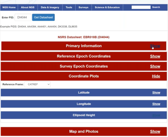
The boxes below highlight a few of the options NGS is considering. The box “Data Delivery – Prototype” is an example provided by Smith during his webinar. It should be noted that the images of the prototype are not included in the downable slides, but they are part of the video. The images presented in this column are screen captures from the video.
Data delivery prototype. (Image: NGS)
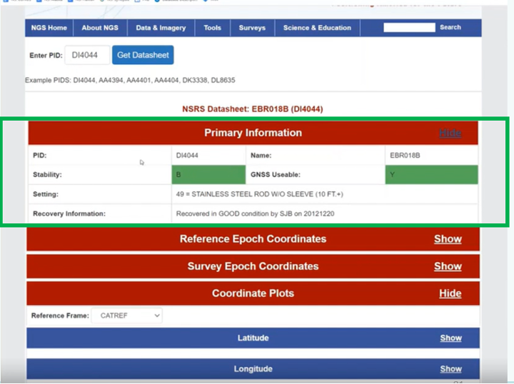
The box below provides some of the basic information of a mark, such as its PID, name, stability, GNSS usable code, setting and the latest recovery information. Again, this is a prototype, so users should feel free to send feedback to NGS. NGS wants to generate a usable product, and is interested in user feedback.
Primary information prototype. (Image: NGS)
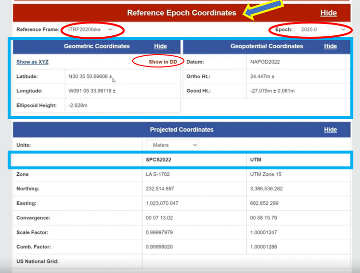
As previously stated, NGS is implementing a two-track approach to coordinates: publishing REC and SEC. The box below provides the REC information of a mark when a user clicks the “Show” button. As shown in the diagram, the reference frame and epoch are provided, as well as the geometric coordinates (latitude, longitude, ellipsoid height) and geopotential coordinate information (NAPGD2022 orthometric height and geoid height).
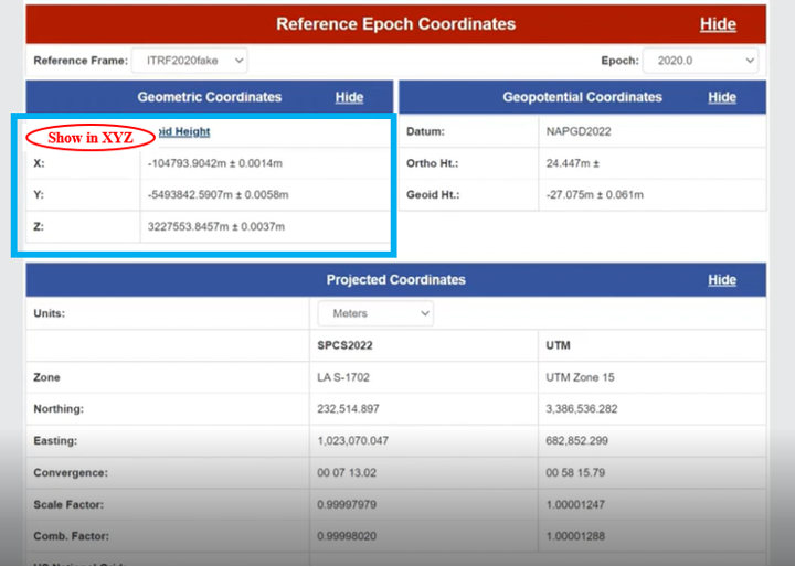
NGS provides an option for individuals who want the geometric coordinates in the X, Y, Z format (see the box below). Remember, this is only a mockup of a prototype, to give us an idea of the direction NGS is going with its data delivery system in the new, modernized 2022 NSRS.
REC Shown in X,Y,Z. (Image: NGS)
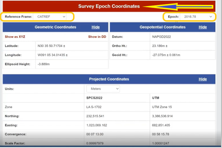
Similar to the REC, the prototype includes SEC. For a mark, the latter are different from the former because SEC are computed at the epoch of the survey observations (see the box below).
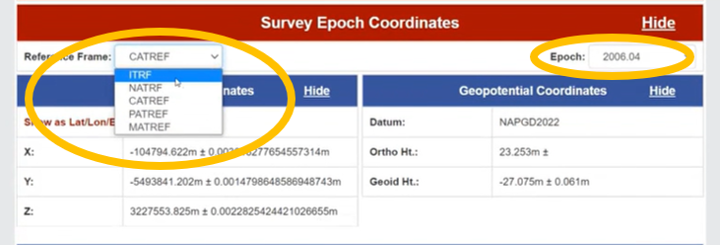
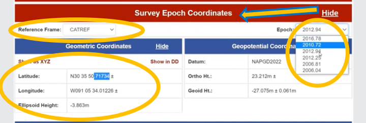
The box titled “SEC in CATRF – Prototype” is an example of a mark in the CATRF reference frame and the survey epoch of 2012.94. As indicated in the diagrams, users will be able to select the reference frame (ITRF, NATRF, CATRF, PATRF and MATRF) and the survey epoch.
SEC in CATRF – Prototype
Option to Select Survey EpochOptions to select reference frame (Images: NGS)
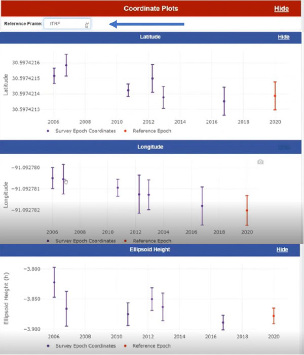
Another feature of the data delivery system is that it provides plots of a mark’s survey epoch coordinate values at different epochs. In the example shown in the box below, the plots provide values of a mark’s latitude, longitude and ellipsoid heights based on each survey epoch data. The user can select various reference frames of the mark to understand the change based on the reference frame.
Coordinate plots in ITRF prototype. (Image: NGS)
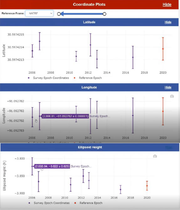
The box below clearly shows a slope in the changes in coordinates based on survey epochs, especially in the longitude. This is the plate rotating in time. You can see the changes in latitude, longitude and ellipsoid height in the NATRF reference frame for the same mark. The latitude and longitude plots do not show a slope because the plate rotation is removed using a model to change from the ITRF reference frame to the NATRF reference frame. That said, the ellipsoid height plots look the same because the rotation model does not change the ellipsoid height.
Coordinate plots in NATRF prototype. (Image: NGS)
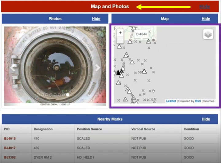
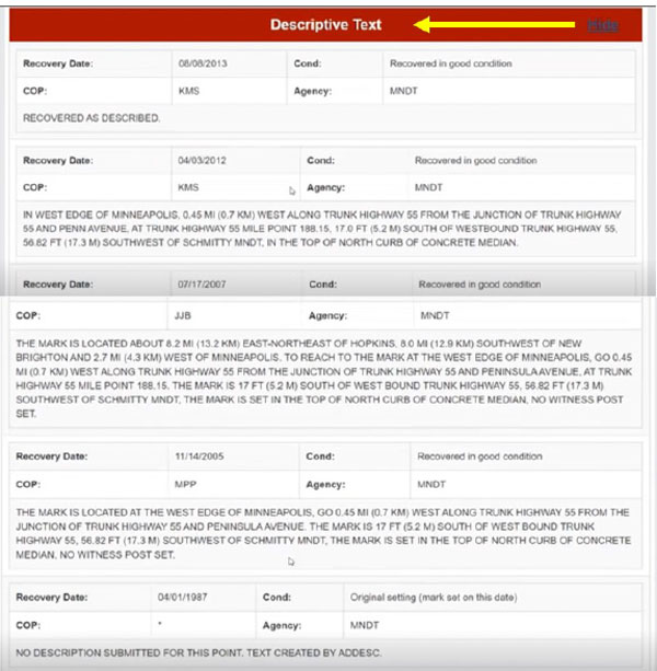
The prototype also provides maps, photos and descriptive text of the mark.
Map and photos of a mark in the prototype. (Image: NGS)Descriptive text prototype (Image: NGS)
Some of this data delivery output may seem familiar to users who have used the NGS beta routines (see the box below).
Beta Routines
Beta routines (Image: NGS)
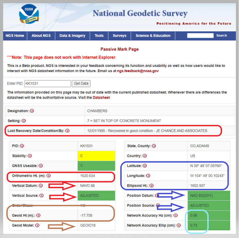
For example, the Passive Mark Page Webtool provides the coordinate information for a mark. My October 2020 column described the tool is detail. See below for an example of the passive mark tool.
Beta Passive Mark of KK1531 (Image: NGS)
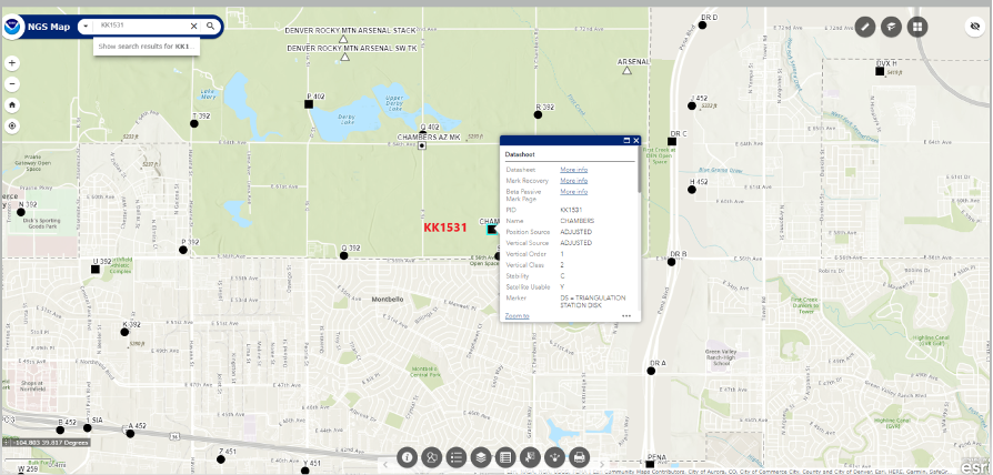
The NGS Beta Map routine enables users to link to NGS datasheets, the passive mark tool and mark recovery, as well as connect to OPUS Shared Solutions and the NOAA CORS Network. See below for an example. It also provides a measuring tool, multiple basemaps and the ability to export data. My December 2021 column described the NGS Beta Map in detail.
Example of NGS Beta Map Routine for KK1531 (Image: National Geodetic Survey)
Only three years remain before the release of the new, modernized NSRS. I encourage everyone to try all of the beta products, and download Dru Smith’s June 6 webinar for a better understanding of the agency’s current thoughts on how it will provide data to users in the new, modernized NSRS. As for all the NGS beta products, the agency would like users to try the tools and provide feedback on what they liked and what they didn’t like, as well as any additional information you need or would like to see. The NGS is trying to develop tools useful to everyone, but that won’t be possible unless they hear from users.
The following statement on NGS beta products explains how to provide feedback and why it is important:
“This is a beta product. NGS is interested in your feedback concerning its function and usability as well as how users would like to interact with NGS datasheet information in the future. Email us at [email protected].”
My February column explained why it is important to account for horizontal movement of marks everywhere, and not just in areas influenced by active crustal movement due to earthquakes such as Southern California.
It provided information about the NOAA CORS Network (NCN) rates of movement based on International Reference Frame of 2014 (ITRF2014) coordinates and horizontal velocity information. It highlighted reports from the National Geodetic Survey (NGS) that describe models that will facilitate users transferring coordinates between reference frames and dealing with intra-frame movement between marks based on surveys performed at different epochs.
NAPGD2022 orthometric heights will primarily be accessed through GNSS technology.
As I stated in my February column, this is not just a horizontal positioning issue. In this month’s column, I address estimates of vertical movement that will have to be accounted for in the new, modernized National Spatial Reference System (NSRS).
NAPGD2022 will provide gridded models for North America (that includes CONUS, Alaska, Hawaii, the Caribbean, Canada, Mexico, Central America and Greenland), American Samoa and Guam/Commonwealth of Northern Mariana Islands (CNMI). My previous columns have described the NAPGD2022 in detail. The revised NOS NGS 64 report mentioned that NAPGD2022 will be built upon ITRF2020. It states that NAPGD2022 will operate equally well in any of the four new terrestrial reference frames developed as part of the new, modernized NSRS in 2022.
As I stated in previous columns, orthometric heights in NAPGD2022 will be defined through GNSS ellipsoid heights and GEOID2022. This means NAPGD2022 orthometric heights will primarily be accessed through GNSS technology. GEOID2022 will be defined in a manner that best fits global mean sea level at the epoch of NAPGD2022.
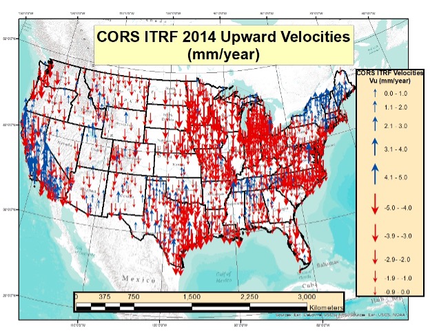
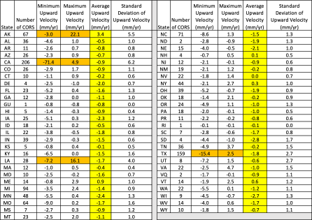
As in my previous column, to better visualize the potential size of the vertical movement, I used the CORS ITRF2014 coordinates and velocities from the NGS website to create plots depicting the upward velocity (Vu) values for CORS that are designated as operational and have computed velocities. [Note: I use the term upward because that is how it is reported on the NGS CORS website under the tab labeled “position and velocity.” The term upward velocity means movement in both directions — negative is downward and positive is upward.] The box below shows maximum, minimum, average and standard deviations of upward velocity values for each state and territory of the United States.
Table of ITRF 2014 Upward Velocities of US CORSs
The upward velocity values are not as systematic as the horizontal velocity values, and they are significantly smaller. I have highlighted the average value velocity column. As indicated in the table, the values vary from state to state, but they are all small relative to the horizontal movement values. (See my previous column for plots depicting the horizontal values.)
What is interesting is the range of values in some states. For example, Alaska and California have a very large range — understandable because of the active earthquakes and other movement that occur in these states. Also, Louisiana and Texas have a very large range due to local subsidence.
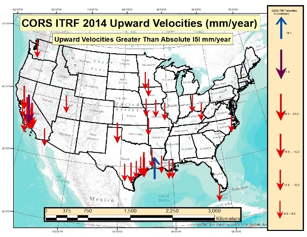
I decided to highlight the values for the conterminous United States (CONUS) in two separate plots. The box “Upward Velocities (Vu) Between +/–5 mm/year in CONUS” depicts upward velocities (Vu) between +/–5 mm/year in CONUS. The box “Upward Velocities Greater than Absolute Values of 5 mm/year in CONUS” depicts upward velocity values greater than +/–5 mm/year.
Upward Velocities (Vu) between +/- 5 mm/year in CONUS
Image: Dave Zilkoski
It’s obvious that most of the vertical movement values are between +/–5 mm/year in CONUS. There are some large values in California, Louisiana and Texas. This is highlighted in both plots.
Upward Velocities (Vu) Greater than Absolute Values of 5 mm/year in CONUS
(Image: Dave Zilkoski)
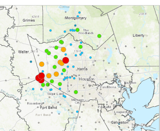
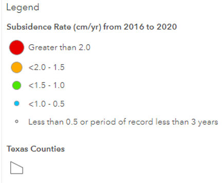
As indicated in the plots, some of the values exceed 10 mm/year. In five years, the heights of marks in these regions could potentially change by 5 cm. An example of the potential subsidence in the Houston-Galveston, Texas, region is depicted in the box below. As indicated in the plot, some marks are subsiding greater than 2 cm/year. That means in five years the marks in that region could have subsided more than 10 centimeters.
Estimate of Subsidence in the Houston-Galveston, Texas, Region
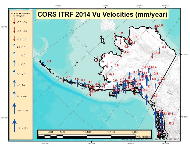
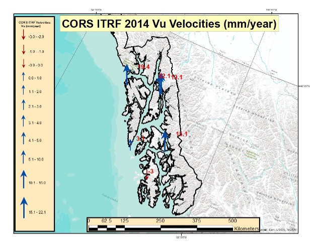
The box below depicts the values in Alaska. Most of these values indicate that the marks are uplifting. Some of these values exceed 10 mm/year. Once again, height coordinates in some regions will potentially change 5 cm in five years. I generated a separate plot for the southeastern region of Alaska. (See the box titled “Upward Velocities (Vu) in Southeastern Alaska.”)
Upward Velocities (Vu) in Alaska [All Values]
Image: Dave Zilkoski
Upward Velocities (Vu) in Southeastern Alaska [All Values]
Image: Dave Zilkoski
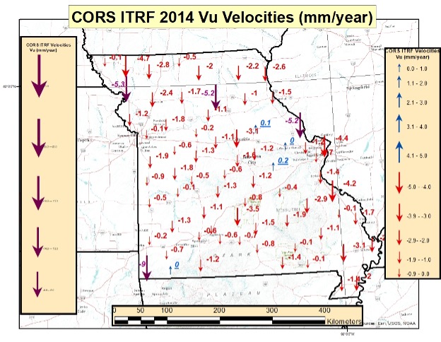
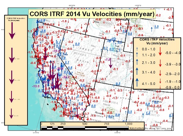
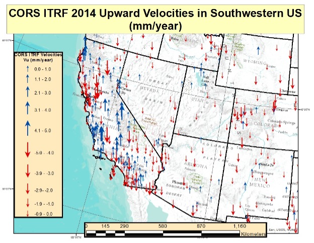
As I did in my previous columns, I prepared several plots that depict the upward velocities in various regions of the United States. See the boxes below for North Carolina, Missouri Southwest U.S. The plots indicate that the magnitude of the vertical movement varies from state to state, as well as within the states.
CORS ITRF 2014 Upward Velocities (Vu) in Missouri [All Values]
Image: Dave Zilkoski
CORS ITRF 2014 Upward Velocities (Vu) in Southwest U.S. [All Values]
Image: Dave Zilkoski
CORS ITRF 2014 Upward Velocities (Vu) in Southwest U.S. [Values Between +/- 5 mm/year]
Image: Dave Zilkoski
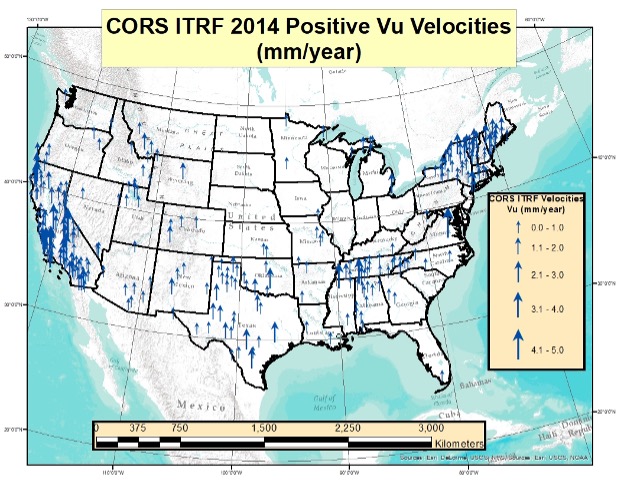
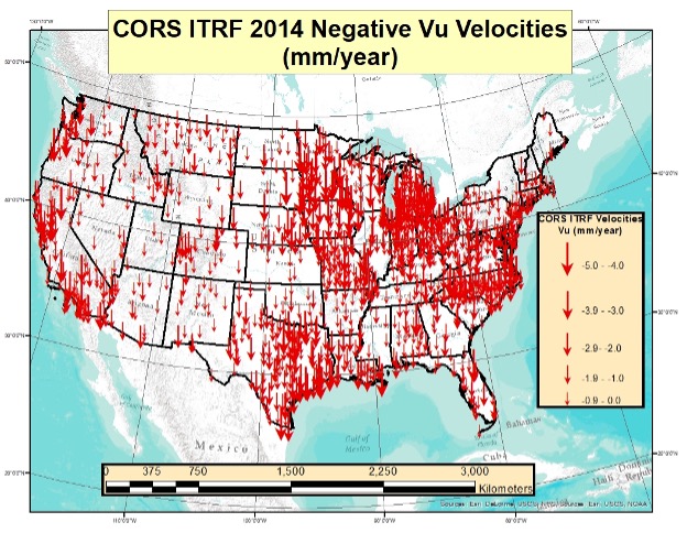
I also generated plots that separately depict the positive and negative upward velocities for the conterminous United States. There are more negative upward velocity values than positive values.
CORS ITRF 14 Positive Upward Velocities (Vu) in Conterminous U.S. (Values between 0 and 5 mm/year)
Image: Dave Zilkoski
CORS ITRF 2014 Negative Upward Velocities (Vu) in Conterminous U.S. (Values between -5 and 0 mm/year)
Image: Dave Zilkoski
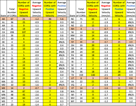
The table below provides the number of CORS with negative upward velocity values and the number of CORS with positive values for every state and territory of the United States. I have highlighted the states and territories that have more positive values than negative values. As you can see, only six states have more positive upward velocities than negative values. Four of the six states are in Northeastern United States.
Table of ITRF 2014 Positive and Negative Upward Velocities for United States
So far, this column has only addressed the vertical movement at the NCN CORS. The values at the sites indicate the potential movement of marks in the area of the CORS. The rates are based on GNSS data and have an estimate of error associated with them.
I’m not sure how NGS will address the vertical movement effects in the new, modernized NSRS. That said, NGS will be monitoring the CORS and looking for trends to help describe the movement at the CORS. These trends will be an indication of what may be happening in the area.
In addition to the movement of individual marks, there are geophysical reasons for changes in the geoid. As I stated in previous columns, orthometric heights in NAPGD2022 will be defined through ellipsoid heights and GEOID2022. Therefore, changes in the geoid model will be very important to users estimating orthometric heights using GNSS.
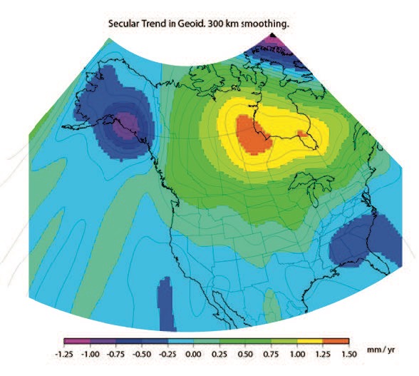
As stated in the NGS 64 report, NGS has set a goal of maintaining geoid accuracy at 1 centimeter (1 standard deviation) in both absolute and differential geoid undulations. Figure 13 from the NGS 62 Report depicts an estimate of the secular change in the geoid. As indicated in the plot, the changes are very small, ranging from –1.25 mm/year to 1.5 mm/year.
What I find interesting is the small negative change in the southeastern United States. There are other drivers for geoid changes. Future columns will address some of these changes and what it means to users.
Figure 13 from NOS NGS 62 Report
Image from NGS website: Blueprint 2 Revised NOAA_TR_NOS_NGS_0064.pdf
Figure 13 – Secular Geoid Change
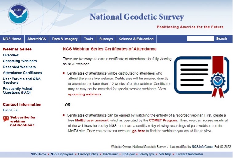
Lastly, I’d like to highlight a new service from NGS: “NGS Webinar Series Certificates of Attendance.” See the box titled “Ways to Earn a Certificate of Attendance.” Basically, users can earn certificates by viewing a webinar after it has been posted by NGS. This is very useful for users who could not attend the original webinar. I encourage all users to check out the site to find out more information about the new service.
Ways to Earn a Certificate of Attendance
Image from NGS website: https://geodesy.noaa.gov/web/science_edu/webinar_series/certificates.shtml
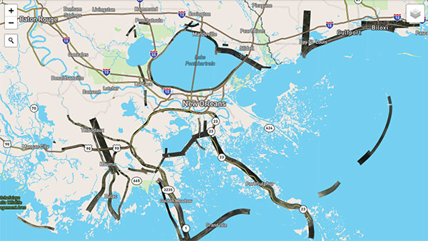
Hurricane Ida assessment imagery and data are now available. Ida was a Category 4 Atlantic hurricane from Aug. 26 to Sep. 4. (Screenshot: NOAA)
Applanix, a Trimble Company, and the National Oceanic and Atmospheric Administration (NOAA) have collaborated to provide critical information to first responders in the wake of Hurricanes Henri and Ida.
Applanix’s high-accuracy direct georeferencing (DG) technology enabled NOAA to quickly collect aerial mapping imagery to
provide valuable disaster remediation information to first responders
demonstrate the value of mapping technology in preparing for and responding to emergency situations such as hurricanes, tornadoes and other disasters.
Within hours of Hurricanes Henri and Ida making landfall, NOAA’s National Geodetic Survey collected post-storm imagery using the latest generation Digital Sensor System (DSS). The sixth-generation DSS, designed and manufactured for Applanix by Lead’Air, is the most powerful to date, thanks to several new features introduced within the solution:
simultaneous full color and near-infrared image capture using high-performance Phase One iXM 100 MP NIR and 150 MP RGB cameras
option to fly the cameras in wide coverage oblique or traditional overhead (straight line down) mode for mapping with uninterrupted measurement
embedded Trimble AP60 GNSS + inertial OEM DG solution for mapping without the need for ground control or aerial triangulation
Applanix POSPac post-processing software featuring the Trimble post-processed CenterPoint RTX correction service (PP-RTX) for centimeter-level mapping without GNSS reference stations
in-air development of raw imagery to JPEG-ready files for creating map products immediately upon landing
Lead’Air’s X-Track flight management, which enables the system to be flown outside of planned flight lines to follow roads, rivers and coastlines.
Applanix’s DG technology suite provides direct GNSS inertial georeferencing, meaning that all pixels in the aerial images taken by NOAA are mapped at their exact location on the ground.
“We have worked with Applanix for nearly 20 years,” said Michael L. Aslaksen Jr., chief of the remote-sensing division, NOAA’s National Geodetic Survey. “The level of sophistication they bring to aerial imagery and mapping keeps our team at the forefront of the industry. Their customer support team is always open to new ideas, new innovations and doing whatever it takes to get the job done.”
First responders have access to this imagery and mapping within 24 hours via the cloud (as does anyone at storms.ngs.noaa.gov) and can map detailed response plans based on highly accurate data highlighting where the greatest need lies.
Access to this turnkey emergency response imagery is available to any federal agency, municipality, insurance company or other entity that depends on highly accurate information to plan for and recover from disasters.
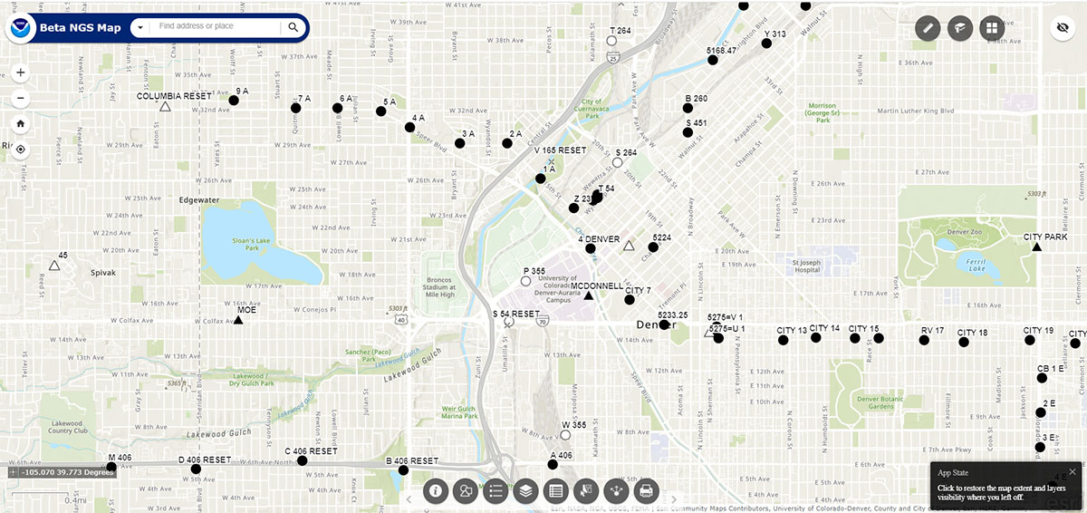
On Nov. 9, the National Geodetic Survey (NGS) announced the release of a new Beta NGS Map. This web application allows users to view multiple datasets that are useful to anyone planning or performing a survey project, or anyone that’s just looking for NGS marks.
The map enables users to access NGS datasheets, OPUS Shared Solutions, and the NOAA CORS Network. It also provides a measuring tool, multiple basemaps, and the ability to export data.
I recently used this tool on my iPhone to locate marks when I was traveling. It’s an amazing tool that is easy to navigate, and a useful tool for identifying marks to be included in a project.
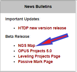
The NGS homepage provides a link to the Beta NGS Map (see below).
Image: NGS Website
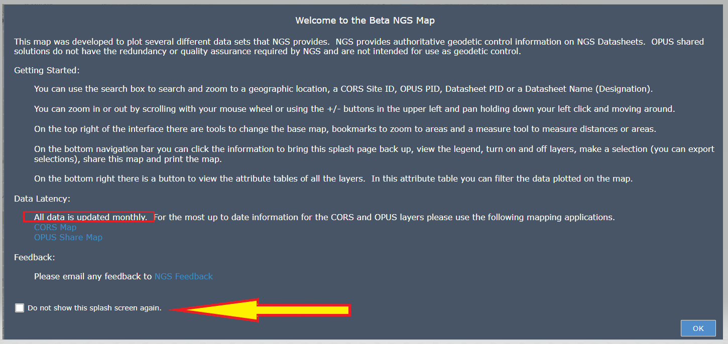
When you first click on the NGS Map link a short narrative appears that provides a brief set of instructions on how to use the map (see below). There’s a box that you can check so that the narrative will not appear every time you access the site. It’s important to note that the data for the CORS and OPUS Shared results are updated monthly. This could be an issue in some instances, therefore users should always check the NGS website for the latest information for the NOAA CORS Network or OPUS Shared map.
Beta NGS Map. (Image: NGS website)
After you click OK at the bottom right of the page, a sample map will appear.
Sample map of Denver region. (Image: NGS website)
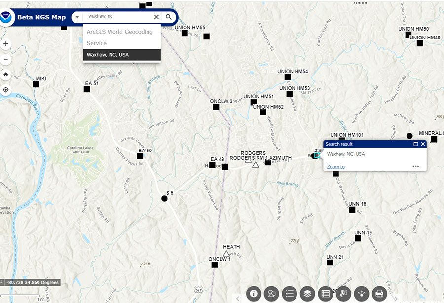
The map allows the user to type in a location (geographic location, CORS Site ID, OPUS PID, Datasheet PID or Datasheet Name) to start a search. See the “Waxhaw, North Carolina, Region” map as an example of entering a geographic location.
Waxhaw, North Carolina, Region. (Image: NGS Website)
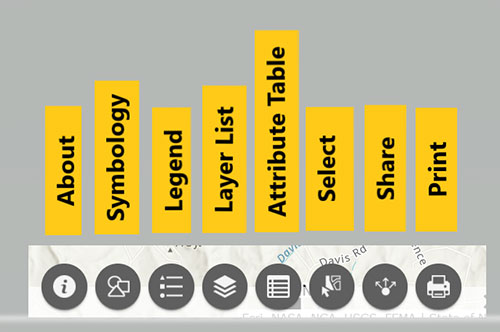
The bottom navigation bar has eight buttons.
List of buttons at the bottom of the map. (Image: Dave Zilkoski)
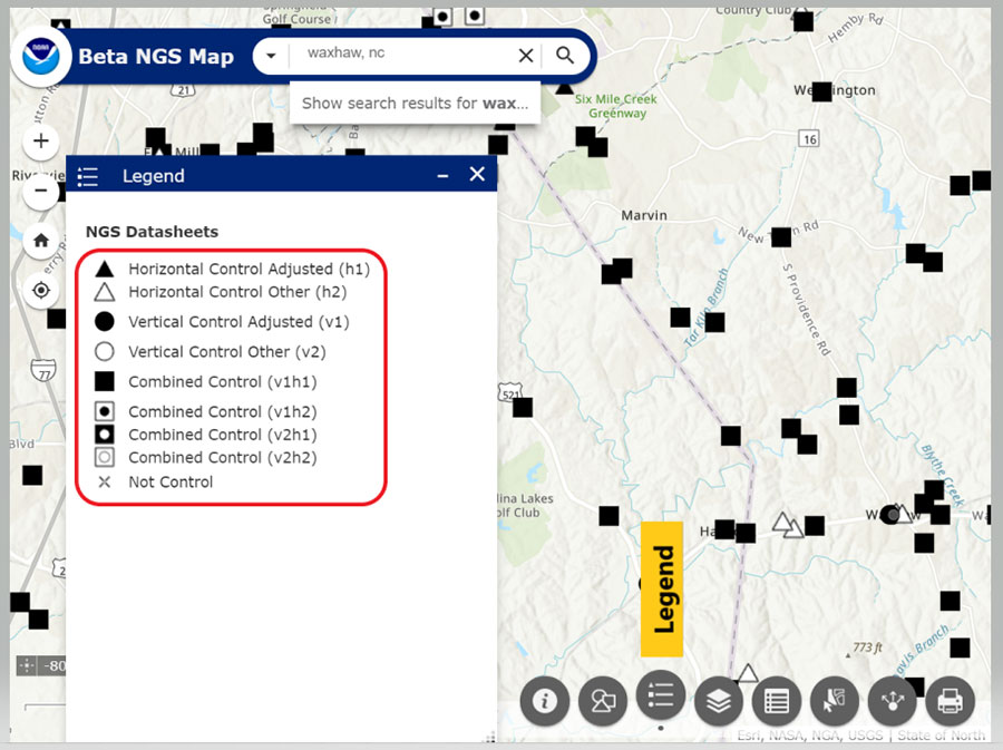
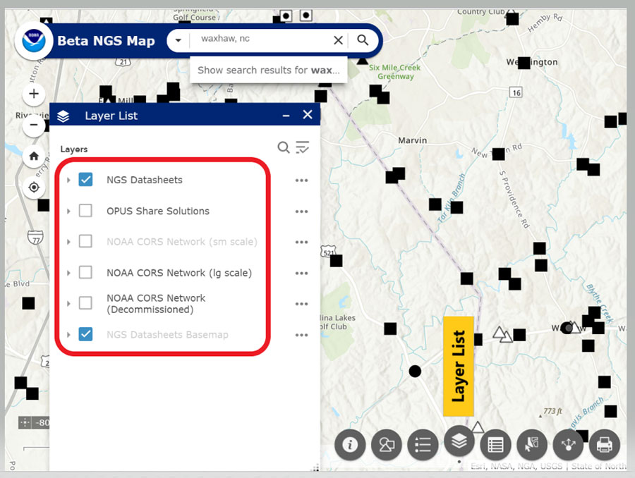
When clicked, a window pops up providing information about that particular button. (For example, see “Map with Legend Information” below.) The legend will include all layers that have been selected. In my example, the datasheet layer was the only layer I had selected (see “Map with Layer Information”.)
Map with legend information. (Image: NGS Website highlighted by Dave Zilkoski)Map with layer information. (Image: NGS website highlighted by Dave Zilkoski)
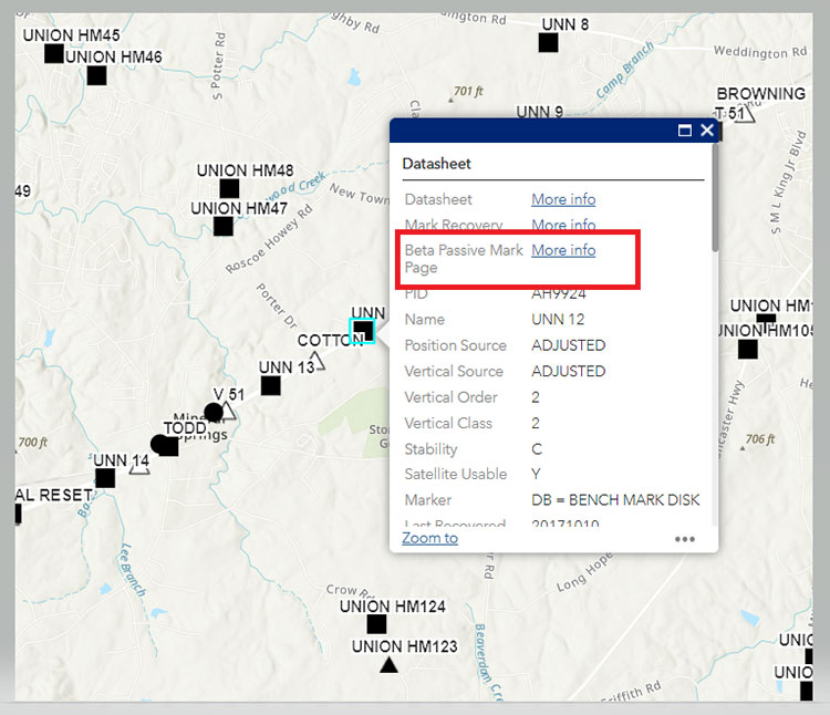
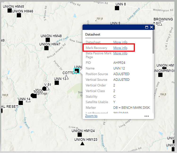
When the user clicks on a symbol, a box will appear with information about the mark. See “Information for Station UNN 12” below.
Information for Station UNN 12. (Image: NGS Website)
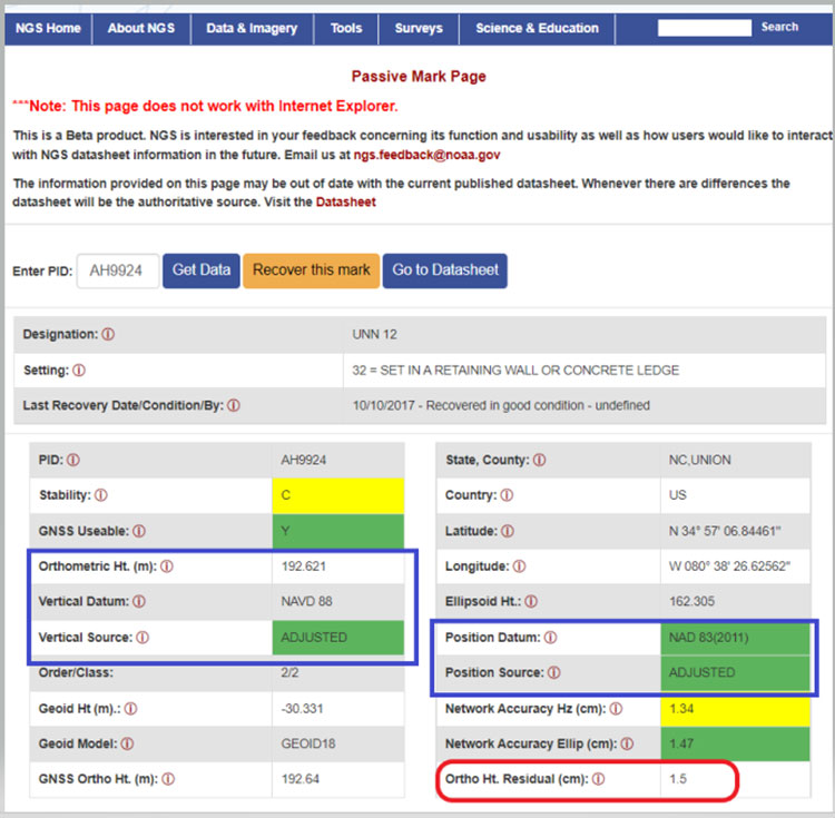
The box contains information from the NGS datasheet as well as a link to the actual NGS database. A nice feature of this webtool is that it provides a link to NGS’s Beta Passive Mark webtool. My October 2020 Survey Scene column highlighted the features of the NGS’s Passive Mark tool. The box captioned “Passive Mark Page for Station UNN 12” is an example of the tool. I’ve highlighted several items important to individuals planning surveys, such as the mark’s coordinates, datums and source, and the Orthometric Height residual (the difference between the estimated geoid height and the modeled hybrid geoid height).
Passive Mark Page for Station UNN 12. (Image: NGS website)
Another great feature is that the user can click on the Mark Recovery link to provide the latest recovery information for a mark (see the box titled “Mark Recovery Link for Station UNN 12 “).
Mark Recovery Link for Station UNN 12. (Image: NGS website)
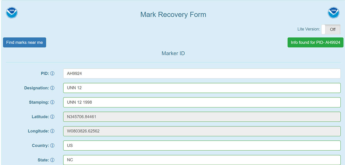
When a user clicks on the More info link for the Recovery Mark option, a Mark Recovery Form is provided for the user to enter the recovery information for the mark. The routine fills in the fields based on the current data in NGS’s database (see the box titled “Mark Recovery Form for Station UNN 12”). The user can enter changes or new information about the mark. This information is very important to users planning surveys. Just because a mark has been occupied by GNSS in the past doesn’t mean that it’s still a good station for occupation by GNSS. The environmental conditions around the mark could have changed since the last time it was occupied; for example, new buildings and/or growth of trees may now obstruct the GNSS signals.
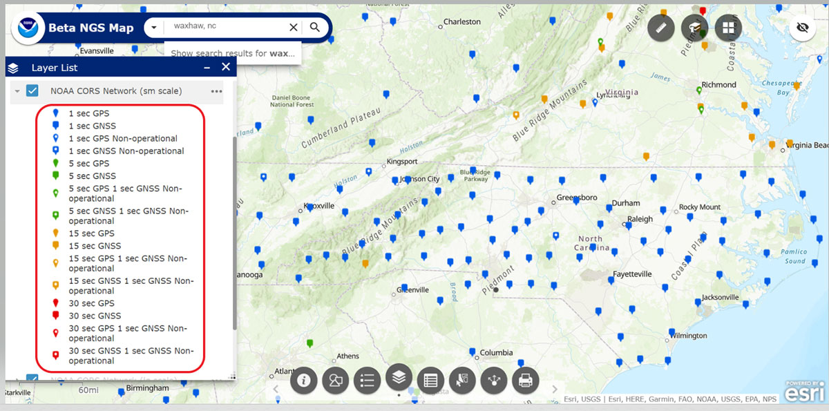
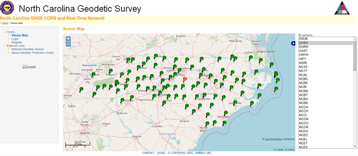
As previously stated, the NOAA CORS Network is one of the layers available. The box titled “Map of NOAA CORS Network in the North Carolina Region” depicts the locations of the NOAA CORS in North Carolina. The layer list provides some of the attributes of the CORS, such as the sampling rate and which GNSS signal are collected at the site.
Map of NOAA CORS Network in the North Carolina Region. (Image: NGS website)
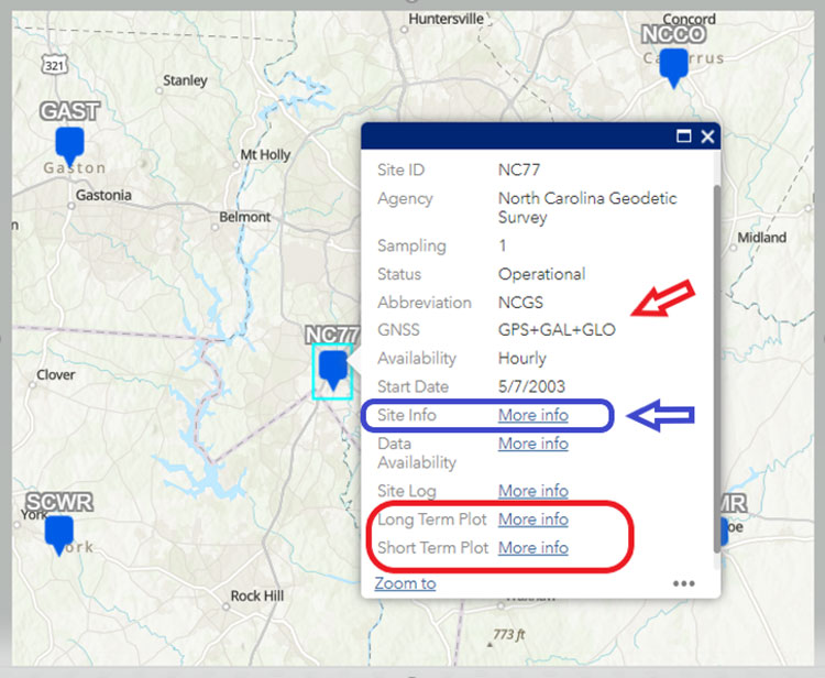
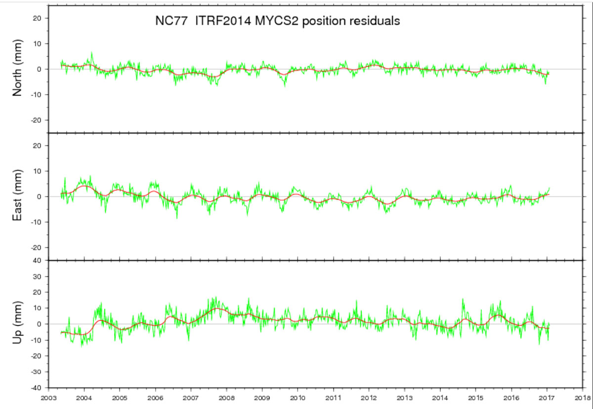
When a user clicks on a specific CORS, a box appears with information for that particular CORS. I’ve highlighted several items in the box titled “Information on CORS Site ID NC77.” In my example, CORS NC77 collects GPS, Galileo,and GLONASS data. Also, users can obtain long-term and short-term plots of the CORS.
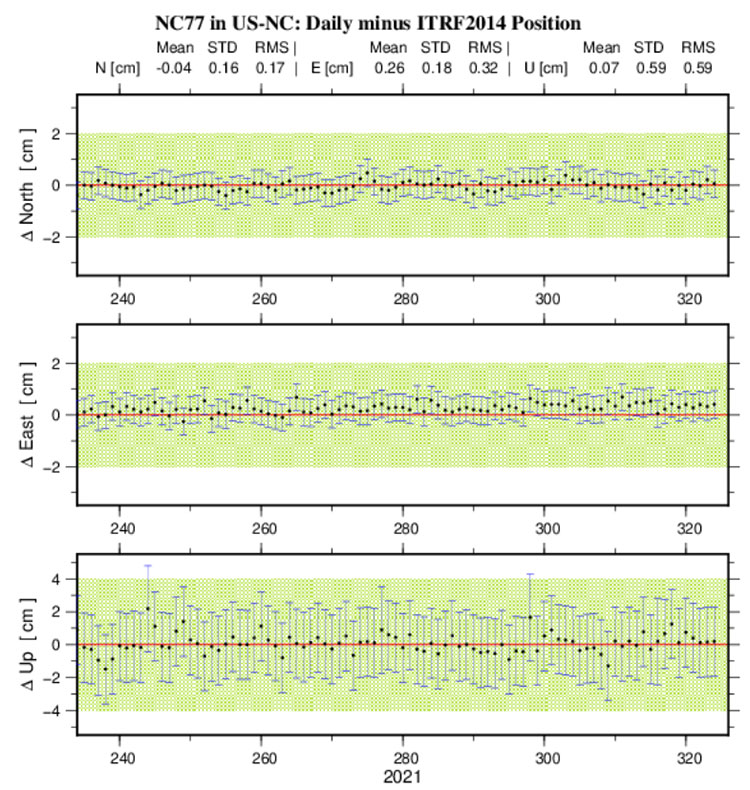
Once again, this feature is important to users planning and performing GNSS survey projects. As in the other features, clicking on the More Info link will bring up the plots. The plots for CORS NC77 are provided in the boxes titled “Long-Term Plot Information on CORS Site ID NC77” and “Short-Term Plot Information on CORS Site ID NC77” below.
Information on CORS Site ID NC77. (Image: NGS website)Long-Term Plot Information on CORS Site ID NC77. (Image: NGS website)
In the short-term plot, the red line is the published position, and the green hashed area is the tolerance of the NGS position, that is +/- 2 cm horizontal and +/–4 cm vertical. All the error bars are 1 sigma values. This information is useful when selecting NOAA CORS to be included in a survey project.
The short-term plot contains the mean, standard deviation and RMS values for the north, east and up components of the site. When planning a GNSS project, users typically identify several NOAA CORS to be included in the project. However, not all CORS are equal.
I evaluate CORS using the following criteria:
Designated as “operational”
Computed (i.e., measured) velocities rather than modeled (i.e., predicted) velocities.
“Consistent” data depicted in short-term time-series plots.
Network accuracies ~1 to 1.5 cm horizontally and less than ~2 to 3 cm in ellipsoid height.
Clicking on the More Info button for Site Info of NC77 provides a webpage where most of this information can be obtained.
Before conducting any post-processing, the analyst should ensure that all CORS included in the project have data for all of the occupations and that the station’s short-term plots indicate stability.
Short-Term Plot Information on CORS Site ID NC77. (Image: NGS website)
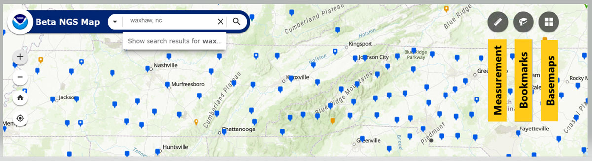
Tool buttons are situated in the top right section of the map. Included are a measurement tool to measure distances between marks and areas, a bookmarks tool to zoom to areas, and a basemaps tool to change the basemap. See the box titled “Useful Tools.”
Useful tools. (Image: NGS website)
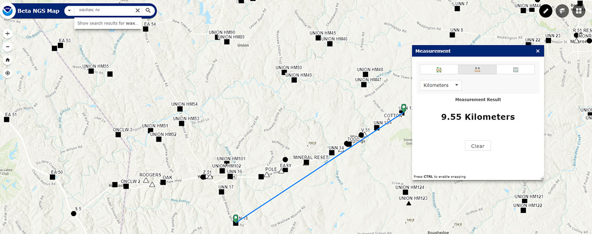
Some users may find the measurement tool helpful when planning a survey. The box titled “Using the Measurement Tool” is an example of measuring the distance between two stations.
Using the measurement tool. (Image: NGS website)
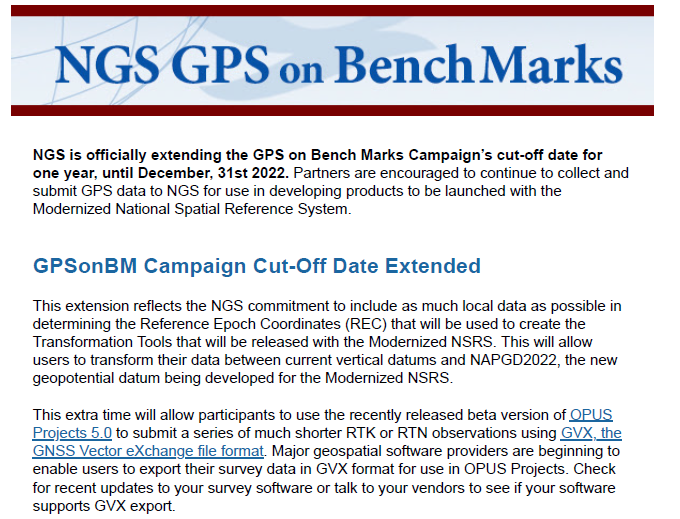
The last item that I’d like to highlight is that on Nov. 18, NGS has officially extended the GPS on Bench Marks campaign’s cut-off date for one year until December 31, 2022. See the box titled “NGS GPS on Bench Marks Notice.”
NGS GPS on Bench Marks Notice. (Image: NGS website)
NGS is anticipating that this extra time will allow users to provide additional GPS on Bench Marks data using the recently released beta version of OPUS Projects 5.0.
As stated in the NGS news release, this extension reflects NGS’ commitment to include as much data as possible in determining the Reference Epoch Coordinates (REC) that will be used to create the Transformation Tools to be released with the Modernized NSRS.
I encourage everyone to try the new Beta NGS Map. As in all of NGS beta products, NGS would like users to try the tools and provide feedback on what they liked and what they didn’t like. They are trying to develop tools useful to everyone, but that won’t be possible unless they hear from users.
On Sept. 16, the National Geodetic Survey (NGS) released the latest beta version of OPUS, called Beta OPUS Projects 5.0. This version of OPUS now accepts real-time kinematic data and post-processed GNSS vectors from vendor software. See the box titled “Beta OPUS Projects 5.0 Webpage” on the website.
As stated in the announcement, NGS has developed a file format for submitted real-time kinematic (RTK) data and post-processed GNSS vectors from vendor software to NGS. It is denoted as GNSS Vector Exchange Format (GVX). This format enables NGS to incorporate the data into its GNSS processing routines.
This is similar to the original Receiver Independent Exchange Format (RINEX) developed for making post-processing more efficient when combining GNSS data from manufacturers outputting raw GPS data in varying file formats. In my opinion, this is a significant improvement to NGS’s OPUS web utility.
Users can obtain background information about the GVX file format by clicking the link GVX file format. More detailed information about the GVX format can be obtained by clicking on the Documentation link.
Basically, GVX is a standardized format for exchanging GNSS vectors derived from GNSS survey data using any manufacturer hardware and software results (see the box titled “Excerpt from Documentation of GVX”). NGS designed the format so that it included all of the necessary data (including metadata) of a GNSS vector for incorporation into a survey network for performing a least-squares adjustment.
To this end, this document proposes a new standardized file format known as the GNSS Vector Exchange Format (GVX). GVX aims to provide a standard format for exchanging GNSS vectors derived from varying GNSS survey methods and manufacturer hardware. The file format includes all of the necessary data of a GNSS vector for inclusion in a survey network for least squares adjustment, as well as metadata which describes the vector. The format is meant for any type of GNSS vector, whether it was derived in real-time or from baseline post-processing. GVX has been written in extensible markup language (XML). XML was chosen because it was designed to carry and store data in plain text format, it is easy to expand and/or upgrade to new operating systems, and it can be read by both humans and machines.
A sample GVX file can be obtained by clicking on the link titled “Example of GVX file, project day 066, day 052, day 053, day 054.” As NGS states in the documentation, the output can be read both by humans and machines. What’s important is that it can be read by machines so the information can be incorporated into software programs. GNSS vendors have all the information they need to generate the output file to enable users to import the data into OPUS Project 5.0. Users will have to contact their software providers to determine whether their software routines generate the GVX output files.
As I previously mentioned, this new option in OPUS Projects 5.0 is a significant improvement because many surveyors use RTK networks to obtain coordinates of marks. It will also facilitate the occupation of benchmarks with GNSS equipment to support the NGS 2022 Transformation tool. North Carolina, my home state, has a real-time network (RTN) that includes 96 GNSS CORS. (See the box titled “NC GNSS CORS and Real-Time Network.”) Currently, the North Carolina GNSS CORS and RTN has 4584 RTN service subscriptions.
I could not find a current list of public RTK networks in the United States, but I did locate a Jan. 7, 2014, GPS World article by Eric Gakstatter that provided a list of public RTK base stations in the country. It’s not up-to-date, but it highlights that, more than seven years ago, more than half of the U.S. states had some kind of public RTK network. I would like to update the table, so I’d appreciate receiving information on the status of any public RTK network. Please feel free to send me an email at [email protected].
California Real Time Network (CRTN) (single baseline). Plate Boundary Observatory. Single baseline.
Colorado
Mesa County (Trimble network) and Plate Boundary Observatory (single baseline).
Florida
Florida Department of Transportation. Leica network.
Idaho
Plate Boundary Observatory (single baseline).
Indiana
Indiana Department of Transportation. Leica network.
Iowa
Iowa Department of Transportation. Leica network.
Kentucky
Kentucky Transportation Cabinet. Trimble network.
Louisiana
Louisiana State University. Trimble network.
Maine
Maine Department of Transportation. Trimble network.
Massachusetts
Massachusetts Department of Transportation. Leica network.
Michigan
Michigan Department of Transportation. Leica network.
Minnesota
Department of Transportation. Trimble network.
Mississippi
University of Southern Mississippi. Trimble network.
Missouri
Missouri Department of Transportation. Trimble network.
Montana
Plate Boundary Observatory (single baseline).
Nevada
Washoe County. Trimble network. Las Vegas Valley Water District. Leica network. Plate Boundary Observatory (single baseline).
New Mexico
Plate Boundary Observatory (single baseline).
New York
New York Department of Transportation. Leica network.
North Carolina
N.C. Department of Environment and Natural Resources. Trimble network. $500 one-time sign-up fee.
Ohio
Ohio Department of Transportation. Trimble network.
Oregon
Oregon Department of Transportation. Leica network. Plate Boundary Observatory (single baseline).
South Carolina
South Carolina Geodetic Survey. Public but charges a usage fee. Trimble network.
Tennessee
Tennessee Department of Transportation. Public but charges a usage fee. Topcon network.
Texas
Texas Department of Transportation. Public but only available to TxDOT employees and TxDOT contractors. Trimble network.
Utah
Utah Automated Geographic Reference Center. Public but charges a usage fee. Trimble network. Plate Boundary Observatory (single baseline).
Vermont
Vermont Geodetic Survey. Trimble network.
Washington
Washington State Reference Network (Seattle Public Utilities). Trimble network. Public but charges a usage fee. Pierce County (Leica Network). Plate Boundary Observatory (single baseline).
West Virginia
West Virginia Department of Transportation. Trimble network.
Wisconsin
Wisconsin Department of Transportation. Trimble network.
Wyoming
Plate Boundary Observatory (single baseline).
Why do I believe that this new option in OPUS Projects 5.0 is so important? Because it facilitates the incorporation of accurate GNSS-derived ellipsoid and orthometric heights into the National Spatial Reference System (NSRS). With the development of improved algorithms, the results of coordinates computed using GNSS CORS/RTNs are more accurate today than ever before. During the last decade, there have been many studies analyzing GNSS data to estimate the accuracy values of coordinates from RTN data.
A study titled “Accuracy of GNSS Observations from Three Real-Time Networks in Maryland, USA” by Daniel Gillins, Jacob Heck, Galen Scott, Kevin Jordan and Ryan Hippenstiel presented at FIG Working Week 2019 in Hanoi, Vietnam, April 22–26, 2019, provided a comparative evaluation on the accuracy of three independent RTNs constructed with differing hardware and software. Their study was based on 486, 5-minute duration GPS + GLONASS network RTK (NRTK) observations. The results indicated that repeat NRTK vectors could be combined to meet 1 cm horizontally and 2 cm vertically (ellipsoid height) accuracies at 95%. confidence. See the box below. It should be noted that the repeat observations should be observed at different times of the day (for instance, separated by > 2–3 hours), as well as, in my opinion, if possible at least more than two different days.
A total of 486, 5-min duration, GPS+GLONASS NRTK observations were collected on nine bench marks distributed over a 4,000 square km area with rovers connected to three different RTNs in Maryland. Each RTN was developed with equipment and software from a different manufacturer, yet all three RTNs performed similarly in terms of accuracy. When differenced with coordinates from a static GNSS survey campaign, the horizontal and vertical RMSE of the NRTK-derived coordinates was 2.3 cm horizontally and 4.5 cm vertically at 95% confidence. Repetitive NRTK vectors on each baseline differed between ± 2.4 cm horizontally and ± 3.4 cm vertically at 95% confidence. As a final accuracy evaluation, hybrid survey networks consisting of repeat NRTK vectors and baseline solutions from post-processing static GPS data collected at RTN base stations and CORSs were adjusted by least squares. Prior to adjustment, the VCV matrices of the vectors were scaled by variance-component estimation. Adjustment of hybrid survey networks with four repeat NRTK vectors per bench mark produced network accuracies at 95% confidence for the adjusted coordinates at all bench marks less than 1 cm horizontally and 2 cm vertically (ellipsoid height).In addition to the benefits of using efficient and accurate NRTK vectors, the hybrid survey network approach makes use of redundant vectors for checking data and avoiding blunders. The approach also provides traceability because the NRTK vectors are tied to an RTN base station which is tied to CORS. Finally, these networks ensure the survey is referenced to the published coordinates of the CORSs which are held as constraints in the adjustment.
Lastly, I would like to remind users that only three months remain until the December 31, 2021, cutoff to submit GPS on Benchmarks data that NGS can guarantee will be analyzed to compute the initial set of 2020.0 Reference Epoch Coordinates (RECs) that will be released with the Modernized NSRS. This initial set of RECs is currently the only set that NGS can guarantee will be used to build the 2022 Transformation Tool. Once the transformation model is finalized, the NAVD 88 – NAPGD 2022 transformation values will be locked in and will not be updated as additional sets of RECs are computed. If you have questions or concerns about this cut-off date, please contact your NGS Regional Geodetic Advisor, or drop NGS a line at [email protected].
Beta OPUS Project 5.0 is a web-based tool that makes it easier to submit data to NGS. I would encourage NSRS users to occupy as many benchmarks with GNSS equipment and submit the data to NGS before the Dec. 31 deadline. Not only will these data help in improving the transformation model, but the marks will be included in the first computation of Reference Epoch Coordinates (RECs). You can obtain information about Reference Epoch Coordinates in NGS’s NOAA Technical Report NOS NGS 67 publication titled “Blueprint for the Modernized NSRS, Part 3: Working in the Modernized NSRS.” A future column will address the different types of coordinates that will be distributed by NGS with the modernized NSRS.
The U.S. Department of Transportation (DOT) and the U.S. Coast Guard Navigation Center (NAVCEN) will hold the 61st meeting of the Civil GPS Service Interface Committee (CGSIC) on Sept. 20-21.
The meeting will be conducted at the St. Louis Union Station Hotel in St. Louis, Missouri, in conjunction with the Institute of Navigation’s 2021 ION GNSS+ conference.
The 61st CGSIC meeting will also be broadcast live online to provide a virtual option. This is a unique opportunity for anyone in the world with access to a computer to attend these public meetings of the U.S. Civil GPS program. CGSIC meetings are free and open to the public.
The three subcommittees of the CGSIC will meet on Sept. 20: Timing; International Information; and Surveying, Mapping, and Geosciences.
Summaries of the subcommittee meetings will be presented to the CGSIC plenary session Sept. 21 with a keynote address by Juliana Blackwell, director of NOAA’s National Geodetic Survey (NGS).
In one of my previous columns, I described the National Geodetic Survey’s (NGS) plans for replacing the North American Vertical Datum of 1988 (NAVD 88) with the North American-Pacific Geopotential Datum of 2022 (NAPGD2022).
As stated in the NOAA Technical Report NOS NGS 64 Blueprint for the Modernized NSRS, Part 2: Geopotential Coordinates and Geopotential Datum, November 2017, recently revised in February 2021, orthometric heights in NAPGD2022 will be defined through ellipsoid heights and GEOID2022. This means NAPGD2022 orthometric heights will primarily be accessed through GNSS technology.
Like NAPGD2022, in the next update of the International Great Lakes Datum, denoted as IGLD (2020), the heights in the Great Lakes Region will be developed from GNSS and a gravity model. Unlike NAPGD2022, where users will be estimating GNSS-derived orthometric heights, IGLD (2020) users will be estimating GNSS-derived dynamic heights using GNSS and a gravity model.
Promote a better understanding of geodesy as a science;
Create a better appreciation of the value of geodetic surveys and thus encourage greater use of such surveys;
Promote geodetic surveys by individuals, government, and private organizations;
Foster the adoption of uniform standards and procedures for completing geodetic surveys;
Promote the processing, publishing, and disseminating of geodetic survey data and information;
Promote programs for testing, calibrating, and evaluating geodetic equipment;
Further the development and implementation of the Global Navigation Satellite System (GNSS) for geodetic, land surveying, and land information system applications;
Inform the membership of new technical developments by meetings of the association and publications in Surveying and Land Information Science (SaLIS);
Promote educational programs in geodesy, geodetic surveying, and related fields;
Cooperate with other similar organizations, both national and international, in support of the science of geodesy;
Encourage the use of geodetic surveys and mathematical coordinate systems in establishing Public Land Survey System (PLSS) corners
As stated above, AAGS cooperates with other similar organizations, both national and international, in support of the science of geodesy. AAGS is a voting member of FIG, which means AAGS has the opportunity to nominate and vote for elected officials, and develop policy that is important to all surveyors and mappers.
The theme of the FIG Working Week 2021 virtual conference was “Smart Surveyors for Land and Water Management: Challenges in a New Reality.” FIG Commission 5 focuses on meeting the highest level of accuracy for positioning and measurement (see box titled FIG Commission 5). Five 90-minute sessions described some of the efforts of FIG Commission 5.
“FIG Commission 5 focuses on meeting the highest level of accuracy for positioning and measurement. It provides the tools, techniques and procedures to educate and train surveying professionals everywhere. Appropriate methodology for data collection and processing are required to be successful in an era of global, integrated geospatial data.”
These sessions raised surveyor awareness of cutting-edge technology, techniques and procedures for using geodetic data and enhanced global cooperation and standardization in conformance with the ideals expressed by the United Nations resolution for a Global Geodetic Reference Frame. There were many good papers on positioning and measurement presented at the virtual meeting. Readers can obtain a list of presentations and papers at this website.
A paper by Jacob Heck, U.S National Geodetic Survey, and Michael Craymer, Canada Geodetic Survey titled “Updating the International Great Lakes Datum: Enabling the Integration of Water and Land Management in the Great Lakes Region” should be of interest to many U.S. and Canadian surveyors. The box below provides a link to the abstract, paper, handouts and video of the presentation.
05.1 – Managing the Land/Water Interface: WGS84 vs. the ITRS
Commission: 4 and 5
Chair: Dr. Mohd Razali Mahmud, FIG Commission 4 Chair, Malaysia
Rapporteur: Dr. Daniel Roman, FIG Commission 5 Chair, United State
Jacob Heck (U.S.) and Michael Craymer (Canada):
Updating the International Great Lakes Datum: Enabling the Integration of Water and Land Management in the Great Lakes Region (11046)
[abstract] [paper] [handouts] [video]
The International Great Lakes Datum uses dynamic heights instead of orthometric heights traditionally used for elevations on land. Figure 4 from Heck and Craymer’s FIG paper, illustrates the difference between orthometric and dynamic heights. See box titled “Figure 4 from FIG Paper by Heck and Craymer.” As described by Heck and Craymer, “The dynamic height represents the difference in potential above the reference surface and is the same at all points on a level surface. Orthometric height represents the actual physical distance above the reference surface which may change due to differences in gravity caused by the convergence of equipotential surfaces toward to the poles. Dynamic heights are therefore required for the proper management of water levels and flows in compliance with international regulations and treaties.”
Figure 4 from FIG paper by Heck and Craymer
Figure 4. Dynamic heights,HD, and orthometric heights, H. (from FIG 2021 paper by Heck and Craymer)
I would like to highlight, as described in the paper and stated in the summary, that access to the future IGLD will be primarily through GNSS techniques.
The International Great Lakes Datum provides a framework for water level management in the world’s foremost resource of surface freshwater. The current datum, IGLD (1985), is being updated and replaced by IGLD (2020). This updated datum will be fundamentally different in terms of definition and access to the datum. The datum will be identical to the new NAPGD2022 North American geopotential datum and will be compatible with the existing CGVD2013 (if not identical as well) at the reference epoch of 2020. IGLD (2020) is expected to be released in 2025 at about the same time as NAPGD2022. Access to both frames will be primarily through GNSS techniques. This will lead to more consistent heights across the entire Great Lakes region. Further information about the IGLD update can be found on the Coordinating Committee website.
This new paradigm is important for anyone who works in the Great Lakes region. Actually, it is important to anyone that surveys in the United States, because this new paradigm will also be used to access the North American-Pacific Geopotential Datum of 2022 (NAPGD2022). Anyone following my columns knows this is the future, and that the National Geodetic Survey (NGS) is leading the way in the United States by modernizing the National Spatial Reference System (NSRS).
Another section that I’d like to highlight is in the box titled “Excerpt from Heck and Craymer Paper on IGLD.”
For IGLD (2020), the geoid height, N, will be provided by GEOID2022 which will be used to define NAPGD2022 and the expected update to CGVD2013. IGLD (2020) dynamic heights will therefore be equivalent to dynamic heights in NAPGD2022 and CGVD2013 at the 2020 reference epoch. For IGLD (2020) heights of water levels, hydraulic correctors may also need to be applied.
An important advancement in the development of the new IGLD and North American datums will be the availability of an accurate crustal velocity model that can propagate ellipsoidal heights between different reference epochs. This will enable heights determined at any epoch to be propagated back to the adopted 2020 reference epoch used for IGLD (2020). This will effectively obviate the need to update the entire IGLD datum for the effects of GIA for a much longer period of time, except for incremental improvements to the velocity model and updates to the reference epoch.
It’s important for users to know that the IGLD (2020) dynamic heights will be equivalent to dynamic heights in NAPGD2022, and an accurate crustal velocity model will be used at any epoch to propagate back to the adopted 2020 reference epoch. The box titled “Determining Heights in IGLD (2020)” is an excerpt from Heck and Craymer’s FIG paper that describes the process that will be implemented for estimating GNSS-derived dynamic heights in the updated IGLD (2020).
In previous realizations of IGLD, spirit leveling was used to determine geopotential numbers which were converted directly to orthometric heights that could then be converted to dynamics heights using equation 4 (𝐻𝐷 =𝐶/𝛾45).
In the geoid-based IGLD (2020), heights will be primarily determined through GNSS techniques which provide a direct measure of ellipsoidal height. Although spirit leveling is more accurate over shorter distances, GNSS methods combined with an accurate geoid model are capable of providing more accurate heights over moderate to longer distances at a small fraction of the cost of leveling.
An orthometric height, H, above the geoid is obtained from a GNSS-derived ellipsoidal height, h, above the reference ellipsoid using the geoid height or undulation, N, of the geoid above the reference ellipsoid. This is represented by the simple equation:
𝐻 = ℎ − 𝑁 (5)
Using equations (2) – (5), the dynamic height can be obtained from the GNSS-derived ellipsoidal height using:
𝐻𝐷 =(𝑔̅ ∗ (ℎ − 𝑁))/𝛾45 (6)
For IGLD (2020), the geoid height, N, will be provided by GEOID2022 which will be used to define NAPGD2022 and the expected update to CGVD2013. IGLD (2020) dynamic heights will therefore be equivalent to dynamic heights in NAPGD2022 and CGVD2013 at the 2020 reference epoch. For IGLD (2020) heights of water levels, hydraulic correctors may also need to be applied.
An important advancement in the development of the new IGLD and North American datums will be the availability of an accurate crustal velocity model that can propagate ellipsoidal heights between different reference epochs. This will enable heights determined at any epoch to be propagated back to the adopted 2020 reference epoch used for IGLD (2020). This will effectively obviate the need to update the entire IGLD datum for the effects of GIA for a much longer period of time, except for incremental improvements to the velocity model and updates to the reference epoch.
As stated by Heck and Craymer, hydraulic correctors may also need to be applied to meet IGLD (2020) International policies, procedures and regulations. Information on IGLD (1985) hydraulic correctors can be found on NGS Geodetic Tool Kit Page.
Another paper presented at FIG Working Week that would be of interest to surveyors is a paper on establishing a geoid-based vertical datum given by Dan Roman, Chief Geodesist at NGS (see the box below). Again, the abstract, paper, handouts and video can be downloaded from the link.
05.1 – Managing the Land/Water Interface: WGS84 vs. the ITRS
Commission: 4 and 5
Chair: Dr. Mohd Razali Mahmud, FIG Commission 4 Chair, Malaysia
Rapporteur: Dr. Daniel Roman, FIG Commission 5 Chair, United State
Roman Daniel (USA): Determining an Optimal Geoid-Based Vertical Datum (10876)
[abstract] [paper] [handouts] [video]
Roman discusses the concept of establishing an International Height Reference System (IHRS) so all countries could provide physical heights across their boundaries and over the oceans (see the boxes titled “Excerpt from FIG Paper by Dan Roman” and “Summary from FIG Paper by Dan Roman “). I’ve highlighted several sections that are important to establishing a IHRS.
The IHRS is relatively recent compared to the ITRS. Ihde et al. (2017) discussed plans for unification of heights globally, which were updated more recently in Sanchez et al (2021). Just as ITRF realizations are made within the ITRS, there will be IHRF realizations made within the IHRS. The key concept here is that positions will first be realized in the ITRS and then expressed in the IHRS. This means that GNSS-accessed geodetic coordinates will determine your position in a realization of the ITRF. Using those ITRF coordinates, geopotential values will be determined from an equivalent IHRF model based above a datum of W0 = 62,636,853.4 m2 s-2. This effectively gives your position in the Earth’s gravity field, which is a physical height. In adopting such a model then, all countries might provide consistent physical heights across their national boundaries and over the oceans.
There is a great deal of activity in modernizing how geospatial data are collected, processed and maintained globally. International agreements are in place to have everyone adopt the Global Geodetic Reference Frame to facilitate geospatial data transfer. The approach will be to realize coordinates in the International Terrestrial Reference Frame and then obtain physical heights from the International Height Reference Frame. Countries may adopt any realization of the ITRF but are restricted to a single geopotential value in the IHRF – W0 = 62,636,853.4 m2 /s2. If comparisons to local tide gauges demonstrate this is not optimum for national definitions of a vertical datum, then an alternate geopotential datum can be determined based on an approach that requires supplemental information.
GNSS-observations on multiple tide gauges will establish local Mean Sea Level and any variations due to Topography of the Sea Surface. A model of the TSS would be required to remove TSS effects at tide gauges to determine the geodetic coordinates of MSL. Use of a geopotential model enhanced by locally obtained gravity data would yield the geopotential number(s) at tide gauge(s). Assuming multiple tide gauges, then an average or some statistical analysis might be made to determine the optimal geopotential value to select as a geoid.
NGS’s new modernized NSRS will be compatible with the concept of an International Height Reference Frame. As stated in Roman’s paper, a recent article by Laura Sanchez, et.al, describes a strategy for the realization of the IHRS (see box below.)
Authors: Laura Sánchez, Jonas Ågren, Jianliang Huang, Yan Ming Wang, Jaakko Mäkinen, Roland Pail, Riccardo Barzaghi, Georgios S. Vergos, Kevin Ahlgren and Qing Liu1
Abstract
In 2015, the International Association of Geodesy defined the International Height Reference System (IHRS) as the conventional gravity field-related global height system. The IHRS is a geopotential reference system co-rotating with the Earth.
Coordinates of points or objects close to or on the Earth’s surface are given by geopotential numbers C(P) referring to an equipotential surface defined by the conventional value W0 = 62,636,853.4 m2 s−2, and geocentric Cartesian coordinates X referring to the International Terrestrial Reference System (ITRS). Current efforts concentrate on an accurate, consistent, and well-defined realisation of the IHRS to provide an international standard for the precise determination of physical coordinates worldwide. Accordingly, this study focuses on the strategy for the realisation of the IHRS; i.e. the establishment of the International Height Reference Frame (IHRF). Four main aspects are considered: (1) methods for the determination of IHRF physical coordinates; (2) standards and conventions needed to ensure consistency between the definition and the realization of the reference system; (3) criteria for the IHRF reference network design and station selection; and (4) operational infrastructure to guarantee a reliable and long-term sustainability of the IHRF. A highlight of this work is the evaluation of different approaches for the determination and accuracy assessment of IHRF coordinates based on the existing resources, namely (1) global gravity models of high resolution, (2) precise regional gravity field modelling, and (3) vertical datum unification of the local height systems into the IHRF. After a detailed discussion of the advantages, current limitations, and possibilities of improvement in the coordinate determination using these options, we define a strategy for the establishment of the IHRF including data requirements, a set of minimum standards/conventions for the determination of potential coordinates, a first IHRF reference network configuration, and a proposal to create a component.
I have highlighted several statements in the box titled “FIG Working Group 5.3.” This working group is focused on issues associated with implementing vertical control based on an International Height Reference Frame (IHRF). NGS is working with these groups to ensure that the United States height system will be compatible with the rest of the world.
I encourage everyone to visit the FIG website and explore the papers given during 2021 FIG Working Week. Here is a list of the FIG Commissions. For more information can be obtained on each commission by clicking on the Commission’s title.
Before the American Congress on Surveying and Mapping (ACSM) disbanded, the four-member organization collaborated to convene annual surveying and mapping conferences in the United States. Topics similar to those presented at FIG Working Week were presented at these conferences. I became a member of ACSM in 1972 and learned a lot from attending and participating in these conferences.
Since these ACSM conferences are no longer being held, I encourage users of geospatial data and GNSS technology to participate in professional societies such as AAGS to enhance their understanding and knowledge of new technical developments in the field of geospatial positioning and measurement. As the current president of AAGS, I am biased, but a benefit of AAGS membership is access to the Surveying and Land Information Science (SaLIS)journal that publishes new technological developments related to geodesy, surveying, and mapping.
My last column highlighted an ArcGIS web application that incorporates various datasets and data layers to assist surveyors planning vertical control surveys. On Jan, 29, the National Geodetic Survey (NGS) released the latest experimental geoid model, xGeoid20, and a new gravity interpolation tool (see box below, “NGS Releases Annual e& Gravity Interpolation Tools”).
This newsletter will highlight some attributes of these two new products. First, why am I writing about another experimental geoid model. I discussed xGeoid18 in my December 2018 column and xGeoid16 in my June 2017 column. What’s important here is that this will be the last experimental geoid model until 2022, and the dynamic geoid model has also been updated this year in the form of xDGEOID20.
xDGEOID20 is produced by NGS within the Geoid Monitoring Sƒervice (GeMS) and is part of the new NAPGD2022. Therefore, users only have a few more years to understand the differences between the hybrid geoid model that is being used today to estimate GNSS-derived orthometric heights and the gravimetric geoid model which will be used to estimate North American-Pacific Geopotential Datum of 2022 (NAPGD2022) GNSS-derived orthometric heights.
NGS also announced a new gravity tool, denoted as “The Experimental Gravity Model 2020 (xGRAV20).” xGRAV20 is designed to provide a full-field gravity value and a digital elevation model height at a-specified location. The xGRAV20 model will be important to users that are computing leveling-derived orthometric heights consistent with NAPGD2022.
It is important to note that the xGEOIDs provide a preliminary but increasingly-accurate view of the changes expected from the upcoming NAPGD2022. Also, the xGEOID20 geoid model is the first combination of the geoid models computed by scientists at NGS and Canadian Geodetic Survey (CGS). One unique element to xGEOID20 is that the differences between the A and the B model are due to the contribution of the GRAV-D airborne gravity and differences in methodology.
The National Geodetic Survey (NGS) has published annual experimental geoid (xGEOID) models since 2014. Each of these experimental geoids demonstrate the improvements provided by the addition of airborne gravity data (GRAV-D data) and by the refinement of geoid computation methods.
As the image above indicates, the xGEOID20 is available over a very large area. The box below lists the latitude and longitude boundaries of the areas where xGeoid20 is available.
Areas Where xGeoid20 Model Is Available. (Image: NGS)
To use the xGeoid20 Interactive Computation Page, the user can click on the “ACCESS TOOL” button below the map or the Interactive Computation button on the left side of the webpage (see the image above, “Experimental Geoid Models 2020 (xGEOID20)”). I’d like to highlight a statement that NGS added as a note on the computation page:
Coordinates will be processed as IGS14.
The epoch should be in decimal year format and reflect the user-specified output epoch. If no epoch is entered, the tool will use a default epoch equal to the epoch of the static geoid model, which is currently 2020.00.
The user needs to know that the epoch is used to compute the xDGEOID20 value. I will demonstrate how this works later in this column.
As in past xGeoid interactive computations web applications, the user can submit data in various formats. The box titled “Input Formats Permitted for xGeoid20 Webtool” provides a list of the permitted formats. It should be noted that inputting an ellipsoidal height, epoch and name are optional. However, the default epoch is 2020.00, so if you want a different epoch, you need to enter the date. Also. the program will only compute an orthometric height if the user provides an ellipsoidal height.
Input Formats Permitted for xGeoid20 Webtool. (Image: NGS)
Users have the option of getting the output from the xGeoid20 tool on their computer screen or in the CSV format. The box below is an example of inputting data using the screen option. Once you enter your data, the user clicks on the submit button.
Example of Input Format for Screen Option. (Image: NGS)
The next image shows an example of the output using the screen option. I have highlighted a few numbers that I’d like to address.
Your input in NAD83 (2011) epoch 2010.00 (red). I entered my coordinates as NAD 83 (2011), and it assumed that these coordinates are epoch 2010.0.
Your Result in IGS14 epoch 2020.00 (blue). The routine provides your output coordinates in IGS14, epoch 2020.00. This is the epoch of the static geoid model.
The geoid height of GEOID18 (with respect to NAD83) and the orthometric height in NAVD88 (based on GEOID18) (green). This NAVD 88 value is for comparison purposes only. It is using GEOID18 and provides an estimate of the differences between the future NAPGD2022 and the current NAVD 88. The orthometric height is computed using the following formula: NAD 83 (2011) ellipsoid height (epoch 2010.0} minus GEOID18.
Ortho Height (brown). This is the estimation of the orthometric height using the following formula: IGS14 ellipsoid height (epoch 2020.0} minus xGEOID20A (or B).
Ortho(model)-NAVD88(GEOID18) (purple). These differences are the estimates of the differences between the future NAPGD2022 and the current NAVD 88. It provides the differences for both the xGeoid20A and xGeoid20B model. I look at the B model because it used the GRAV-D data in the development of the model.
Accuracy (yellow). This is the estimated 95% confidence interval for geoid height.
Example of Output Format from Screen Option
xGEOID20 Interactive Computation Output
Note: The GRS80 ellipsoid is used for both NAD83 and IGS14.
N: The geoid height at epoch t0 = 2020.0, which is geocentric and relative to the GRS80 reference ellipsoid.
Accuracy: Estimated 95% confidence interval for geoid height.
DN: The time-dependent geoid change computed between user inputted epoch (t) and t0. To obtain the dynamic geoid height at user inputted epoch (t), add N + DN.
Either Model A or Model B N values may be used for this depending on user preference.
Example of Output Format from Screen Option. (Image: NGS)
The box below shows an example of inputting data using the CSV option.
Example of Output Format from CSV Option
Note: The GRS80 ellipsoid is used for both NAD83 and IGS14.
N: the geoid height at epoch t0 = 2020.0, which is geocentric and relative to the GRS80 reference ellipsoid.
Accuracy: Estimated 95% confidence interval for geoid height.
DN: the time-dependent geoid change computed between user inputted epoch (t) and t0. To obtain the dynamic geoid height at user inputted epoch (t), add N + DN. Either Model A or Model B N values may be used for this depending on user preference.
Example of Input Format for CSV Option. (Image: NGS)
The printed output from the CSV option looks very confusing, but it can be imported into an excel spreadsheet. The headings and values are all separated by a comma so everything falls into the appropriate columns after importing the data (see image below.)
Example of CSV Output Format Imported into Excel. (Screenshot: David Zilkoski)Example of CSV Output Format Imported into Excel. (Screenshot: David Zilkoski)
I stated in the xGeoid20 write up that the dynamic geoid model has also been updated this year in the form of xDGEOID20. This model is produced by NGS within the Geoid Monitoring Service (GeMS) and is part of the new NAPGD2022. For a thorough discussion on GeMS and the time-dependent geoid, view the webinar from NGS’ presentation library. See the box titled “GeMS Webinar by Kevin Ahlgren.”
Also, one of my previous columns described NGS’ GeMS program. The images titled “Examples of the Time-Dependent Geoid Change in Alaska EPOCH 2020.0” and “Examples of the Time-Dependent Geoid Change in Alaska EPOCH 2025.0” show the change in geoid value from Epoch 2020 to Epoch 2025 for two stations in Alaska.
Examples of the Time-Dependent Geoid Change in Alaska EPOCH 2020.0. (Image: NGS)Examples of the Time-Dependent Geoid Change in Alaska, EPOCH 2025.0. (Image: NGS)
First, looking at the box titled “Examples of the Time-Dependent Geoid Change in Alaska EPOCH 2020.0,” the change between NAPGD2022 and NAVD 88 is approximately 1 meter. Users should note that the GEOID12B is used to establish the NAVD 88 height. Alaska was not included in GEOID18. Comparing the two Alaska labeled boxes, the xDGEOID2022 change between 2020.0 and 2025.0 is –4 mm. I will address this topic in more detail in future newsletters.
As stated by NGS news announcement, “The xGEOID models provide a preliminary but increasingly-accurate view of the changes expected from the upcoming North American-Pacific Geopotential Datum of 2022 (NAPGD2022).” NGS has produced many figures that describe the bias and trend between the future NADGP2022 and NAVD 88. In my June 2017 column I provided a plot that depicted the difference between NAPGD2022 and NAVD 88 based on the GPS on Bench Mark dataset. See the image below.
Figure from June 2017 Survey Scene column. Approximate Change Between NAPGD2022 and NAVD 88 Using GPS on BMs Data (units = cm). (Image: NGS)
These figures provide a broad picture of the change but to better understand the changes across the Nation, I used the GPS on Bench Mark dataset, that was involved in the creation of Geoid18 model, to compute an average latitude, longitude, and ellipsoid height for every State. Obviously, this is a fictitious mark but it provides an idea of the average change based on marks that have both a GNSS-derived ellipsoid and a leveling-derived orthometric height. The plot titled “Difference Between the Future NAPGD2022 and NAVD 88” depicts the average difference for each state based on the GPS on Bench Mark data file. These differences were generated using the xGeoid20B values from the output of the xGeoid20 website.
Difference Between the Future NAPGD2022 and NAVD 88. (Image: NGS)
I would encourage everyone to select a couple of marks and compute the differences to understand the change in their particular region. I was the NAVD 88 Project Manager and I informed users of the potential changes between the NGVD 29 and NAVD 88 for about a decade, and I still had surveyors tell me that they didn’t know it was coming. Please take a few minutes to read NGS’ write up on xGEOID20, estimate the differences in your area of interest, and spread the word to your colleagues, friends, and clients.
The last item that I’d like to highlight is that NGS has released a beta version of a surface gravity model consistent with xGEOID20. See the box titled “Experimental Surface Gravity Model 2020 (xGRAV20).” Users can access the beta webtool here.
The box below provides the output using the tools sample data.
Output from Screen Output Format from xGRAV20 Tool. (Image: NGS)
This gravity tool will be important when users want to incorporate leveling-derived orthometric heights into NAPGD2022. We will address this tool in more detail in future newsletters. I want to emphasis that these two web tools are beta sites. As a beta site, users should verify all information from the site. I encourage everyone to access the tool and check out a few of their favorite marks, and then send an email to NGS informing them of what you like, what you would like to change, and what you would like to see added to the tool.
NGS is releasing this tool as a beta product to get feedback from users. They are interested in your feedback concerning its function and usability as well as how users would like to interact with NGS web tools in the future. Email NGS at [email protected].
In conclusion, I want to leave you with a thought about change. When I give presentations and seminars, I usually include a slide that probably expresses the thoughts of many individuals.
My brother once told me:
“If you geodesists did it correctly the first time you wouldn’t have to keep performing adjustments and changing the values. Just do it right the first time.”
He’s a doctor and said he must do it right the first time.
My response to my brother and to everyone else is the following:
If you want to improve you have to be willing to change, and if you want to continue to meet future positioning requirements you need to continually change.
Winston Churchill said it better “To improve is to change; to be perfect is to change often.”