Tag: sensor fusion

  • Inertial performance: Enhanced tightly coupled dead reckoning

    Inertial performance: Enhanced tightly coupled dead reckoning

    Exploring IMU specifications and correlating them to performance of a final product can be daunting, as differences between MEMS sensors are not always apparent. This article presents achievable performances in fusion technology across a range of IMUs among the best in their respective performance categories. 

    The number of available options in inertial navigation systems (INS) has grown substantially over the last several years. Major advances have been made not only in inertial measurement unit (IMU) technology, but also in the ability to exploit sensor information to its fullest extent. In both cases, the largest impact can be seen in the micro-electrical-mechanical systems (MEMS) sensors. MEMS sensors are typically much smaller, lower power and less expensive than traditional IMUs. The net result of these improvements is a proliferation of INS systems at much lower cost than were previously available and, therefore, greatly increased accessibility to technology that has historically seen limited deployment. Selecting the appropriate sensor and fusion solution for a particular application can be very challenging due to the large and confusing spectrum of solutions.

    The IMUs will be examined in the context of new enhancements to sensor fusion algorithms such as the use of INS profiles. The concept of INS profiles applies environment specific constraints to improve performance in certain types of vehicles, or motion profiles. External sensors such as odometers and dual antenna operation can also aid the solution considerably, but will be unused in this analysis except for occasional comparisons. These external aiding sensors are extremely helpful in many cases and are available to use with a proprietary tightly coupled GNSS+INS solution called SPAN, but this paper seeks to evaluate what performance can be achieved without such aids.

    Real-world test results will be examined using a selection of IMUs with the latest SPAN algorithms to illustrate what kind of performance can be achieved with different sensors in difficult conditions. Despite their major advances over the past few years, there are many challenges involved with utilizing MEMS technology to provide a robust navigation solution, particularly during limited GNSS availability or low dynamics. The measurement error characteristics of these devices have improved dramatically, but are still much larger and more difficult to estimate than traditional sensors. Advancements in SPAN sensor fusion algorithms have enabled these smaller sensors to achieve remarkable performance, especially in applications where environmental conditions allow for additional constraints to be applied.

    This testing focuses on the land profile, meaning the constraints applied to a fixed-axle vehicle. The test scenarios were selected in such a way as to provide results for ideal, poor and completely denied GNSS coverage.

    INS Profiles

    GNSS and IMU sensors are only one part of the overall INS system performance. The sensor fusion algorithms used to exploit the available sensor data to its utmost capability are equally as important. In this regard, several improvements have been made to the SPAN INS algorithms to enhance performance under a variety of scenarios.

    The largest addition to the SPAN product line is the introduction of INS profiles. That is, environment- and vehicle-specific modeling constraints can be utilized to enhance the filter performance. For example, the land profile, which will be examined in depth in this article, is intended for use with ground vehicles that cannot move laterally. The assumptions introduced for land vehicles, however, are not necessarily valid for different forms of movement, such as those experienced by a helicopter. Therefore, profiles have been implemented via command, and controlled as required by the user, allowing for maximum performance depending on the application at hand.

    The land profile is analogous to what has historically been identified as dead reckoning. It is a method that uses a priori knowledge of typical land vehicle motion to help constrain the INS error growth. In other words, it makes assumptions on how land vehicles move to simplify inertial navigation from a six-degree-of-freedom system to something closer to a distance/bearing calculation. The land profile takes the concept of dead reckoning, models it as an update type into the inertial filter and adds a few additional enhancements.

    Velocity Constraints / Dead Reckoning. Amongst other optimizations, the land profile enables velocity constraints based on the assumption of acceptable vehicle dynamics. This includes limiting the cross track and vertical velocities of the vehicle. Of all the enhancements, this is the one most colloquially referred to as dead reckoning.

    In its simplest form, dead reckoning is the propagation of a position without any external input. In this forum, external input generally refers to GNSS satellites. Without external input, dead reckoning is inherently dependent on assumptions of velocity and heading to propagate the position. These solutions have evolved by integrating inertial and directional sensors to provide more local input and improve the solution propagation. This also is not a perfect method, however, as inertial sensors have their own errors that grow exponentially over time. The land profile velocity constraints explain the bulk of optimizations SPAN has made to enable dead-reckoning performance in extended GNSS outage conditions.

    Explaining the velocity updates involves using the current INS attitude (  ); the vehicle attitude (  ) is estimated by applying the measured or estimated IMU body to vehicle direction cosine (  ). From this, the pitch and azimuth for the vehicle is estimated.Using the magnitude of the measured INS velocity in conjunction with the derived vehicle orientation, the vehicle velocity is computed, allowing the expected vertical velocity and cross-track to be constrained.

    A velocity vector update is then applied to the inertial filter to constrain error growth. The effects of this method are expected to be most apparent in extended GNSS outage conditions when the INS solution must propagate with no external update information.

    Phase Windup Attitude Updates. Some applications are inherently difficult for inertial sensors due to the fact that these systems are reliant on measuring accelerations and rotations in order to observe IMU errors. When traveling at a constant bearing and speed, separating IMU errors from measurements becomes challenging, so any application that does not provide meaningful dynamics is more demanding on inertial navigation algorithms. This type of condition commonly appears in applications such as machine control, agriculture and mining.

    Gravity is a strong and fairly well known acceleration signal, so the real difficulty in this type of environment is managing the attitude, and especially azimuth, errors. Attitude parameters become difficult to observe when the system experiences insignificant rotation rates about its vertical axis.

    External inputs can be used for providing input during low dynamic conditions when rotational observations are weaker. These are particularly helpful in constraining angular errors and include the same types used to assist in initial alignment: dual antenna GNSS heading, magnetometers, etc. However, as the goal of this testing is to demonstrate the achievable performance from a single antenna GNSS system, this type of external aid was specifically omitted.

    Utilizing a patented technique for determining relative yaw from phase windup, the system is able to distinguish between true system rotation and unmodeled IMU errors during times of limited motion. This is a novel way to extract additional information out of existing sensors rather than adding more equipment and complexity.

    The phase windup update is used to constrain azimuth error growth during low dynamic conditions that are typically not favorable to inertial navigation. However, it does require uninterrupted GNSS tracking and is therefore applicable only in GNSS benign environments. This approach is expected to show the greatest benefit in low dynamic conditions and be directly attributable to azimuth accuracy, but only in conditions where GNSS availability is relatively secure.

    Equipment and Test Setup

    We paired OEM-grade GNSS receiver cards with a selection of IMUs in different performance categories. Since the OEM GNSS platform is capable of tracking all GNSS constellations and frequencies, we configured each receiver to use triple frequency, quad-constellation RTK positioning. The receivers were coupled with a wideband antenna capable of tracking GPS L1/L2/L5, GLONASS L1/L2, BeiDou B1/B2 and Galileo E1/E5b signals.

    Three IMUs were tested: an entry-level MEMS IMU (UUT1), a tactical-grade MEMS IMU (UUT2) and a high-performance fiber-optic gyro-based IMU (UUT3).

    All GNSS receivers and IMUs were set up in a single test vehicle and collected simultaneously for all scenarios. IMUs were mounted together on a rigid frame, and all receivers ran the same firmware build that were connected to the same antenna.

    The tests were conducted using a single GNSS antenna with no additional augmentation sources, such as distance measurement instrument (DMI) or wheel sensor. These are extremely helpful in aiding the solution, but as previously mentioned, this testing seeks to demonstrate the possible performance without the benefit of additional aiding sources. Dependence on aiding sources is a very important distinction when comparing such systems.

    The GNSS positioning mode used was RTK via an NTRIP feed from a single base station with baselines between 5–30 kilometers. This was done to try to minimize GNSS positioning differences between the three systems. L-band correction signals were not tracked, and PPP positioning modes were not enabled.

    A basic setup diagram of each system under test can be seen in Figure 1.

    FIGURE 1. Equipment set-up (not to scale).


    Test Scenarios

    Four test scenarios will be examined using all the equipment and algorithms described above. They are: urban canyon, low dynamics, parking garage and extended GNSS outage.

    The urban canyon test is designed to show the performance of the system in restricted GNSS conditions. The challenge to this scenario is to maintain a high-accuracy solution when GNSS positioning becomes intermittent or even unavailable.

    The low dynamics test is intended to illustrate the benefits of the land profile, and specifically the phase windup azimuth updates in maintaining the azimuth accuracy.

    The parking garage test will show the efficacy of the velocity constraint models over the different IMU classes as the extended outage provides no external information to the INS filter whatsoever. Again, no other aiding sources were used.

    Urban Canyon Test. The urban canyon environment has been and remains one of the strongest arguments in favor of using GNSS/INS fusion in a navigation solution. Because urban canyons are common, densely populated and, of course, a demanding GNSS environment, they represent both an important and challenging location to provide a reliable navigation solution. Typically, they contain major signal obstructions, strong reflectors and complete blockages (depending on the city). For this reason, they provide an excellent use case for INS bridging to maintain stability of the solution.

    During most urban canyon environments, it is typically rare to incur total GNSS outages of more than 30 seconds. Therefore, this scenario examines the stability of the solution in continuously degraded, but not generally absent, GNSS. In this case, the coupling technique of the inertial algorithms rather than quality of the IMU dominates achievable position accuracy.

    The receiver platform is capable of tracking all GNSS constellations and frequencies. This provides a significant benefit to test scenarios, such as the urban canyon, where the amount of visible sky is significantly restricted. In this case, the more satellites that are observable, the more the tightly coupled architecture can exploit the partial GNSS information.

    Though position accuracy between IMUs is less apparent in this condition, attitude results remain separated by IMU quality, which is a major consideration for some mapping applications such as those using lidar or other sensors where a distance/bearing calculation must be done for distant targets.

    Test data for this scenario was collected in downtown Calgary, Canada. The trajectory (Figure 2) includes several overhead bridges for brief total outages and some very dense urban conditions.

    FIGURE 2. Urban canyon test trajectory.

    Table 1 shows the RMS error results of the three systems running both the default and land profiles. The first thing to notice is that the errors are differentiated by IMU category, though the differences are fairly small in the position domain thanks to the tightly coupled architecture. However, because GNSS information is partially available, the differences seen in activating the land profile are fairly modest, especially as the IMU performance rises.

    TABLE 1. RTK RMS errors for urban canyon.

    As the clearest benefits of the land profile are seen on the entry-level MEMS IMU (UUT1), these will be explored graphically in Figures 3 and 4. Figure 3 shows the position domain, and the RMS differences can be seen in a few cases where the default mode errors increased faster than the land profile. An example of this divergence is most obvious around the 1500-second mark of the test during periods GNSS is most heavily blocked.

    Low Dynamics Test. The low dynamics test is designed to emulate conditions experienced by machine control, agriculture and mining applications. In this situation, GNSS availability is generally not the limiting factor and can be used to control the low frequency position and velocity errors of the INS system. The difficulty is managing the attitude, especially azimuth, errors because attitude parameters are very hard to observe without significant rotations or accelerations (Figures 5 and 6).

    The low dynamics test was collected in an open-sky environment and consisted of traveling in a straight line on a rural road for roughly 2 km at an average speed of 10–15 km/h.

    As this type of scenario provides little physical impetus, the azimuth and gyroscope biases are not observable. The reason for this is due to the use of the first-order differential equations to estimate the navigation system errors. Essentially, the differential equations define how the position, velocity and attitude errors change (grow) over time based on each other and the IMU errors. The observability of a particular update is tied to additional states through the off-diagonal elements of the derived transition matrix with the accelerations and rotations experienced by the system.

    The overall RMS solution errors for RTK are provided in Table 2. As evident by the results presented, the position and velocity errors are clearly constrained by the continuous RTK-level GNSS position regardless of whether the land profile is enabled or not. The real differentiator in the land profile is the attitude performance due to the use of phase windup as a constraint. Moreover, the attitude improvements are certainly tied to IMU quality.

    TABLE 2. RTK RMS errors for low dynamics.
    TABLE 3. RTK RMS errors, parking garage (500s).

    UUT1 exhibited a noticeable improvement in the attitude performance, while the higher performance IMUs did not. This is not entirely unexpected as the precision of the phase windup is lower than that of the higher grade IMUs.

    Looking at the data graphically, Figure 7 shows the effect of land profile on positioning performance in this scenario. The two solutions are indistinguishable on the plot, and are all within standard RTK-level error bounds as was indicated in the RMS table.

    Figure 7 shows the attitude accuracy with and without the land profile enabled. Again, the largest gains are seen on the entry-level UUT1, so this is the graphic shown below. This shows how the error peaks of the azimuth estimates are constrained. All the sharp corrections in each plot correspond to the vehicle turning around at the end of each 2-Km line and illustrates how much more powerful a rotation observation can be in azimuth accuracy overall.

    FIGURE 7. UUT1 attitude error (std vs. land).

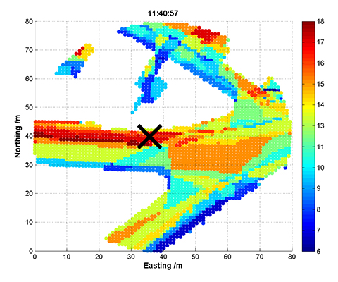
    Parking Garage Test. This test was carried out at the Calgary International Airport and was selected to show the INS solution degradation during extended complete GNSS outages. The test consisted of an initialization period in open sky conditions to allow the SPAN filter time to properly converge, followed by a 500-second period within the parking garage. During the interval within the parking garage there were no GNSS measurements available.

    Figure 8 provides a trajectory of the test environment. The time spent inside the parking structure is evident on the center bottom of the image.

    FIGURE 8. Parking garage test trajectory.

    Unlike urban canyon environments that contain partial GNSS information, this exhibits an extended period of complete GNSS outage. During this type of scenario, the IMU specifications become much more significant. IMU errors directly translate to the duration the solution can propagate before the accumulated low-frequency errors of the IMU grow to unacceptable levels. System performance during the outage degrades according to the system errors at the time of the outage and the system noise. The velocity errors increase linearly as a function of attitude and accelerometer bias errors. The attitude errors will increase linearly as a function of the unmodeled gyro bias error. The position error is a quadratic function of accelerometer bias and attitude errors.

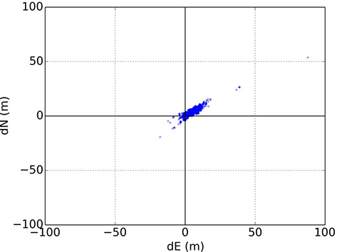
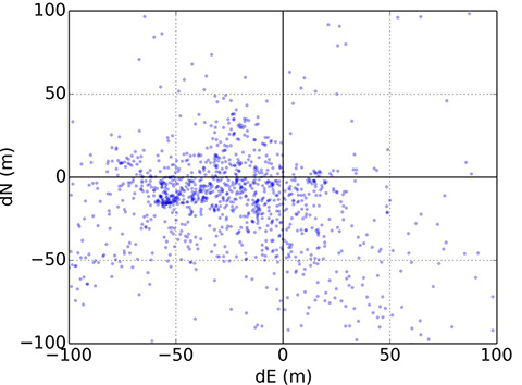
    Position results from each IMU are shown for UUT 1 in Figure 9. This plot shows the error with the land profile on and off. Without the land profile, the second-order position degradation in an unconstrained system is clearly visible.

    FIGURE 9. UUT1 position error (std vs. land ).

    By enabling the land profile, the filter constrains IMU errors by utilizing a velocity model for wheeled vehicles. With the constraints, the position errors are startlingly reduced for UUT1 and then progressively less impactful as the IMU quality increases in UUT2 and UUT3, respectively. This makes sense as the IMU error growth is progressively smaller in those IMUs, so the effect of mitigating them is also reduced.

    Extended GNSS Outage Test. An extension of the parking garage test is to evaluate the performance in a much longer outage. Instead of 10 minutes, an outage of one hour was tested. Also, due to the extremely long GNSS outage bridging, the effects of adding a DMI sensor (odometer) will also be explored as they are able to be used as a major additional aiding source.

    Table 4. Percent error / distance traveled over 1-hour GNSS outage.

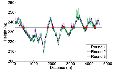
    The most common measure of dead-reckoning performance is error over distance traveled (EDT). Due to the very long duration outages in this test, the errors will be reported in error over distance traveled to conform to the typical reporting method. This test was conducted in a mixture of highways and suburban streets with an average speed of 65 Km/h, incorporating a moderate amount of dynamics.

    This effect can be seen over the duration of the entire outage as well in Figure 9. In this case, the points are the RMS error over several tests. and the light background shroud represents the one-sigma confidence as time progresses. The confidence increases over time as the overall distance traveled also increases.

    FIGURE 10. Land profile EDT with and without DMI aid over 1-hour GNSS outage.

    Results and Conclusions

    In testing a range of IMUs in some challenging scenarios, this paper has sought to illustrate what kind of performance is achievable using each kind of system. An added complexity is looking at what effect certain inertial constraint algorithms have on this solution.

    Although low-cost MEMs IMUs are continuing to greatly improve in quality and stability, the end application is still highly correlated to the overall performance of a selected INS system. For a great many applications, the MEMS devices in combination with a robust inertial filter can meet requirements and provide excellent value. However, some applications continue to require higher end sensors, and possibly post-processing to meet their needs.

    The ability of SPAN to utilize partial GNSS measurements such as pseudorange, delta phase and vehicle constraints means even low-cost MEMs are capable of providing a robust solution in challenging GNSS conditions. However, this tightly coupled integration is limited in cases where GNSS is completely denied or when in low dynamic conditions.

    INS profiles using velocity constraints, phase windup and robust alignment routines have been shown to provide substantial aid to the INS solution in tough conditions, such as GNSS denied or low dynamics. These improvements were shown to exhibit greater impact as the IMU sensor precision decreases. These abilities, in conjunction with the existing tightly coupled architecture of SPAN and the ever-increasing accuracy of MEMS, IMUs indicate that robust GNSS/INS solutions will continue to proliferate at lower cost targets. However, very precise applications such as mapping will continue to rely on higher quality sensors to meet strict accuracy requirements.

    ACKNOWLEDGMENTS

    The authors thank Trevor Condon and Patrick Casiano of NovAtel for collecting and helping to process the data presented in this article, and to Sheena Dixon for her tireless editing.

    Manufacturers

    NovAtel SPAN technology on the NovAtel OEM7 receiver is the testing and development platform for this research. NovAtel OEM7700 GNSS receiver cards and a NovAtel wideband Pinwheel antenna were employed. The inertial units under test were an Epson G320 (low-power, small-size MEMS IMU); Litef μIMU-IC (larger tactical-grade performance IMU still based on MEMS sensors); and a Litef ISA-100C (near navigation-grade IMU using fiber-optic gyros (FOG). Although all are excellent performers in their class and capable of providing a navigation-quality solution, the intent is to show the potential limitations that might arise due to the intended application.


    RYAN DIXON is the chief engineer of the SPAN product line at NovAtel Inc., leading a highly skilled team in the development of GNSS augmentation technology. He holds a BSc. in geomatics engineering from the University of Calgary.

    MICHAEL BOBYE is a principal geomatics engineer at NovAtel and has participated in a variety of research projects since joining in 1999. Bobye holds a BSC. in geomatics engineering from the University of Calgary.

  • Road navigation using multiple dissimilar environmental features

    Look Around

    Road Navigation Using Multiple Dissimilar Environmental Features

    New navigation paradigms combining GNSS and inertial with additional sensors can increase overall reliability and power robust road navigation. A feasibility study tests a barometer, a magnetometer and a camera looking at road signs, and concludes that such sensors examining environmental features can supply the necessary context for frequently traveled or shared routes.

    By Debbie Walter, Paul D. Groves, Bob Mason, Joe Harrison, Joe Woodward and Paul Wright

    Where a robust and reliable position solution is required, it is necessary to combine GNSS with other technologies. Dead-reckoning is only suitable for bridging short outages. For robustness against longer GNSS outages, alternative position fixing techniques are needed. Radio-based signals have been excluded from this study as they are either not yet mature or are, like GNSS, susceptible to jamming, though they may still play a part in the final navigation solution.

    For land navigation in particular, a new approach is therefore needed. Environmental features provide a potential source of location information. These include buildings or parts thereof, signs, roads, rivers, terrain height, sounds, smells and even variations in the magnetic and gravitational fields. Visual navigation technologies are being developed and are likely to be complementary to the feature-matching discussed in this article; however, they will not be directly discussed. The environmental features will be integrated with dead reckoning to provide robust positioning.

    The overall solution is to place hardware within a batch of vehicles, comprising multiple sensors, including a GNSS receiver and sensors for dead reckoning. Road map matching could also be included. During normal usage, the GNSS receiver is used for positioning and a database is updated with the feature information from all the sensors accompanied by location stamps from the GNSS-based position solution.

    As the multiple vehicles travel around an area, the database is built up for these routes. In the event that the GNSS receiver does not receive sufficient signals to maintain an accurate position, the database is called upon for navigation by environmental feature matching. In this scenario, the sensors continue to take measurements and, by combining the knowledge of the last known location, dead reckoning and the sensor’s outputs, the positioning algorithm draws upon the database to estimate a positioning solution. This method is shown in Figure 1 and Figure 2.

    This navigation system relies upon the roads being travelled on a regular basis so that the “maps” created from the sensor’s outputs are kept up to date and therefore valid. The most likely users of this technology would be fleets of vehicles that can share the mapping information. To focus on a typical system, use in emergency vehicles was considered. Knowing your position is vital in an emergency vehicle, and a system that incorporates a back-up to GNSS would be advantageous. The motivation for maintaining a continuous positioning solution is that, when moving within a complex environment, it is necessary to maintain the integrity of the current position. In emergency situations, delays are not acceptable and integrity is vital. There will be no point in time when the vehicle can be delayed to obtain a position fix.

    Although this system will be designed with emergency service vehicles such as ambulances and police cars in mind, it could also be used in wider applications such as fleet management and tracking devices. Ultimately, crowd sourcing or cooperative techniques could be used to pool information from different vehicles equipped with the system. With a very large number of vehicles maintaining the feature database, the system could adapt to changes in the environment very quickly.

    To reliably achieve meters-level positioning across a range of different challenging environments, a paradigm shift is needed. We need to use as much information as we can cost-effectively obtain from many different sources in order to determine the best possible navigation solution in terms of both accuracy and reliability.

    This new approach to navigation and real-time positioning in challenging environments requires many new lines of research to be pursued.

    ROAD EXPERIMENT

    A set of sensors with a GNSS receiver were attached to a car and driven in closed loops around Stoke-on-Trent on multiple road types over multiple days. The loops were repeated three times on each day on four road types and then repeated over three consecutive days. The sensors used can be seen in Table 1.

    Table 1. Sensors used in the road experiments.

    The accelerometer, air quality sensor, barometer, dust sensor, light sensors and microphone interfaced with an Arduino microprocessor which outputted the signals from the sensors to a laptop. The Arduino sensors had a data rate of 20 measurements per second. There was an individual accelerometer (attached to the axel of the vehicle) for use in identifying road texture. There are also accelerometers that form part of the inertial measurement unit (IMU), and these were used for dead reckoning.

    The onset of movement as recorded from the IMU was used to assist in identifying the beginning of each circuit. During the car journeys, there were two experimenters, one to drive the car and another to monitor the sensors. There were 5–10 minutes between each round; during this time, the sensors would be turned off and then restarted. The equipment was designed for the outputs of the sensors to be post-processed.

    The four classes of road were suburban, urban, rural and high-speed road. The route taken and a view from Google Street View showing the general type of landscape traveled through is shown in Figure 3.

    A road experiment travelled the routes, using GPS receivers with the Arduino, video camera and the IMU so that GPS time could be used as a constant for the various sensors.

    WHOLE ROUTE ANALYSIS

    The outputs from the sensors were evaluated initially for their cross correlation over the whole route. This process assessed whether the data from different runs over the same terrain were similar and thus had a high cross correlation. This is vital for this map-building method of navigation. This section deals only with sensors that produce continuous output. The next section discusses discrete features.

    Cross-Correlation Coefficients. The correlation coefficient (see online version of this article for derivation equations) is used to calculate the cross-correlation of two rounds of sensor data. The cross correalation coefficient is a normalized value. If a signal is correlated with itself, at zero offset (autocorrelation) this would give a value of 1; entirely uncorrelated data gives 0. Signals 180° out of phase would give a correlation value of –1.

    The cross-correlation coefficients are shown in Table 2 for all of the sensors. It shows the coefficients for the four different road types using combinations of rounds (round 1 and 2, round 2 and 3 and round 1 and 3 for each three days) from the same days and the average of the coefficients for all the combinations. The sensors with higher coefficients are discussed in more detail in the following subsections. Road signs do not have cross-correlation coefficients; they are treated differently as this is a discrete measurement.

    Accelerometer. The magnitude of the acceleration from a accelerometer triad was used in this experiment as a method of measuring road texture. A zoomed-in section of the acceleration as recorded from the accelerometer against the distance traveled can be seen in Figure 4.

    Figure 4. Profile from accelerometer attached to axle.

    It is difficult to see similarities in the output from the different rounds, although the accelerometer can show movement from stationary to driving and this was used to initialize the sensor outputs from the XSens IMU. This is shown in Figure 5 at 44s.

    Figure 5. Accelerometer data showing vehicle setting off.

    Barometer. The barometer measures height change of the vehicle. This sensor consistently produced the highest cross-correlation coefficient, shown in Figure 6.

    Figure 6. Comparison of height profile over 3 days with minimums set to zero.

    Magnetometer. The magnetometer produced data with distinct spikes caused by various magnetic anomalies in the environment being travelled through. This can be seen in Figure 7 for the high-speed road.

    Figure 7. Vertical axis magnetic field profile for a high-speed road.

    Figure 8 is a zoomed-in section of the magnetometer data from the high-speed road in Figure 7. It shows correlation with an offset of approximately 44m between round 1 and round 3. This is mostly due to synchronization errors between the magnetometer counter and the GNSS receiver clock. This is the reason a second run of the road experiment was completed.

    Figure 8. Zoomed-in section of the vertical axis magnetic field experienced on a high-speed road.

    Microphone. The microphone was able to pick up clear signals when the vehicle was stationary, and the signal seems to be dependent on the speed of the vehicle. Figure 9 shows the profile from the microphone.

    Figure 9. Profile from microphone attached to axle.

    It may be possible to combine this data with the accelerometer or odometer data to develop a clearer picture of what sound is resulting directly from the road surface and what is speed related, although this still may not result in a useful feature for this study.

    Thermometer. Temperature can vary particularly in a rural environment, seen in Figure 10. Similarities are not consistent across environments as seen from cross-correlation values in Table 2 and are likely to change with the seasons and due to weather conditions.

    Figure 10. Temperature profile for rural roads.

    Light Sensor. Four light sensors were used in the experiment: upwards, forwards, left and right facing. Figure 11 shows the data from the upward-facing sensor on the high-speed road. There are distinct events where the light level drops. Many of these instances correspond to gantries (bridge -like structures spanning highways displaying speed limits and other information). These features could be treated as discrete, whereby the sharp dips in light level would be treated as momentary events. Some of the information would be lost in treating the ambient light as discrete, but it would make the feature more robust against changing light levels due to shadowing or cloud cover.

    If light is treated as a continuous feature, it can be seen in Table 2 that the cross correlation was inconsistent. This is partly due to the effects of changing light conditions. On the days with direct sunlight, the light sensor would reach its maximum intensity and be saturated. This can be seen in Figure 11, and this affects the cross-correlation coefficient calculated.

    Table 2. Cross-correlation coefficients for sensor outputs for the four road types.
    Figure 11. The upward-facing light sensor profile for the high-speed road in second experiment day two.

    Feature outcome. Thermometer data has been discounted as although it gave a cross-correlation coefficient of about 0.5 for the rural route, the other routes had lower cross-correlation values. Similarly, the microphone data had moderate success in high speed and rural environments but not in the other two routes. Therefore it will not be taken forward to the next phase although it could be used in the future if further processing was carried out on the data. As with the microphone, the light sensor had cross-correlation values greater than 0.5 in the rural and urban environments but had lower values in the other two. The success of this sensor is more reliant on the weather conditions than the environment type. At the current point this will not be brought forward to the next stage.

    The accelerometer (used to measure road texture) showed no correlation with cross-correlation coefficients of approximately zero (between 0.0 and 0.3). It was useful for use in dead reckoning, but does not illustrate road texture.

    The magnetometer and barometer showed the greatest potential for positioning with the highest cross-correlation values consistent over all the environments. These sensors are taken forward into phase 3.

    DISCRETE FEATURES

    A discrete feature is one where there are environmental events that occur at one position but can repeat multiple times along a route. The discrete feature can either be Boolean (an event occurs or does not) or it can be descriptive (different possible events or the strength of the event). Examples of discrete features include lamp posts, speed humps and shop signage.

    In this paper, the discrete feature that will be discussed will be street signs, although the techniques used are applicable to many discrete features. How the signs are identified will also not be discussed in detail in this paper; instead, focus will be on how a sequence of discrete features is used show consistency across a route.

    SCANNING METHOD

    This section will look at scanning one round to find the region that best matches a region from a different round. Figure 12 illustrates this technique.

    Figure 12. Diagram showing the principle used to scan for best match to a pre-set region.

    The test data is scanned through the reference data. Cross-correlation coefficients are calculated as the test data is scanned through. The aim is to locate the position of the test data using the reference data for which the position is already known. The output of this exercise gives a cross-correlation profile (cross correlation as a function of position).

    This profile can be treated similarly to a probability density distribution of position (although they are not the same) and so gives an idea of the probability of the position at each point in the test data.

    Results. Two rounds from the suburban route are shown in this section as an example of the results achieved with the scanning method. Figure 13 and Figure 14 show the cross-correlation profiles for magnetic field and height for day 3 rounds 1 and 2 on the suburban route respectively. The test data region chosen is centered at 1.6 km into the route. The test data region size was 125 m for 4.5 km reference data.

    It can be seen that the magnetic field has a number of peaks along the route. The peak with the highest cross-correlation coefficient is at the 1.6-km point (which is the correct position). For the height figure, there are many broad peaks at similar cross-correlation values approximately 700 m apart. The height peaks are broader than the magnetic peaks because the terrain height changes more slowly than the magnetic field.

    Ambiguities, Dead Reckoning. The two graphs in Figure 13 and Figure 14 show that there are ambiguities present in both of the features. The majority of the features will have some ambiguities along a route, and so it is important to develop a technique that could mitigate them. One way ambiguities could be mitigated is by using the information available from dead reckoning. The dead-reckoning solution will have a specific position error (which grows with time), and the ambiguities from the features can be reduced by only considering the candidate position within the dead reckoning position uncertainty bounds.

    COMBINING FEATURES

    The quality of position information that can be extracted from a particular feature type varies with location. Thus, a better position solution can be obtained if higher weighting is attributed to higher quality features. Factors that will need to be considered include the precision of position that can be extracted from a feature, the level of ambiguity (Are there multiple candidate positions?) and the reliability (how much measurements vary unpredictably with time).

    There are multiple ways to combine the scores from different features. Initially, there is the decision as to when in the position estimation process to combine the features. There are two ways to do this: Either combine the scores for each feature, or combine the position estimates for each sensor. The following subsections will describe a number of ways of combining the scores before estimating the position. It will be noted if these techniques could also be used to combine position estimates.

    Equal Weighting. A simple combination technique is for each feature score to have equal weighting. The equal weighting used earlier took the two scores and found the average. This way, no single feature will dominate the navigation solution. As the feature scores are not probabilities, the values are not self-weighting, therefore it cannot be presumed that that equal weighting would always provide an optimal position estimation.

    Test Data Weighting. This method takes a set of experimental data and empirically determines the weighting coefficients based on the best position solution in this test dataset. The test data would be used to maximize the score of the combined features using weighting at the correct position. This would have the benefit of using real data to determine the weighting, but its strength is based on how representative the test dataset is to the environments that the car will travel in.

    Environment Weighting. This would detect the environmental context and use this to select an appropriate set of weights. For example, the presence of many Wi-Fi sources would suggest a suburban or urban environment, while a vehicle speed of 31m/s (70 mph/113  km/h) would suggest that the vehicle is likely to be on a highway. Based on this knowledge, it would possible to use a specific weighting coefficient set is developed for that environmental context.

    Cross-Correlation Weighting. This weights each feature according to the characteristics of the cross-correlation coefficients profile obtained using the scanning method described earlier. This enables the weighing to adapt to the quality of the data. Figure 15 shows traits of a set of peaks that affect the confidence in the highest peak being the correct position.

    Figure 15. Weighting nomenclature of actual position shown as blue dotted line.

    Taking the uncertainty in the current position, only peaks that, for example, fall within 3 standard deviations would be evaluated. The characteristics of the tallest peaks compared with the others would be used to determine a measure of confidence for that feature.

    There will be more confidence in the tallest peak (h0) if there is a greater difference between its height and that of the other peaks within the uncertainty range (h1, 2, 3). In Table 3 this is height.

    Table 3. Cross-correlation profile weighting showing average distance from true position of the vehicle and the percentage of times the weighted scanning technique calculated the position within 100 m.

    The next factor is the number of peaks within the uncertainty range (No. Peaks). The more peaks, the less confidence that the correct peak has been chosen as the position estimate.

    The average cross-correlation coefficient within the uncertainty region (γ) would affect the confidence in the estimated position. If the average coefficient value (Av. CC) was similar to that of the highest peak, this suggests insufficient variation in the data being analyzed from that feature.

    Finally, the standard deviation could be used. Calculating how many standard deviation (Std Dev) the highest peak was from the mean could provide a weighting value.

    Each of these characteristics was looked at separately and compared against the benchmark of equal weighting using the scanning method comparing multiple pairs of rounds on different routes. It can be seen in Table 3 that the standard deviation from the mean provided the best weighting outcomes. To optimize the weighting algorithm, it may be that using a combination of these profile characteristics would provide the best position estimation.

    Figure 16 and Figure 17 show examples of cross-correlation profiles; they show high and low confidence respectively. Figure 16 is the cross correlation of data from day three, rounds two and three, on suburban roads. It has a few spaced out peaks over the full profile, and one of the peaks is clearly higher than the others. Figure 17 is the cross correlation of data from day two, round three, and day three, round three, from the high-speed road. It has many similar height peaks all around the value of 0.5.

    Figure 16. Good cross correlation profile; few spaced out peaks with one higher than all other peaks.
    Figure 17. Poor cross correlation profile; many low similar height peaks.

    CONCLUSION

    Environmental features have sufficient variability spatially and stability temporally for a database of features to be developed to create a map of the environment. This supports the hypothesis that it is feasible to map a space and then create a feature-mapping and navigation algorithm using a combination of environmental feature sensors, a GNSS receiver and sensors for dead reckoning.

    FUTURE WORK

    The next step of the project is to develop a feature-matching, mapping and navigation algorithm that incorporates inputs from the multiple sensors, a GNSS receiver, map-matching and sensors for dead reckoning. The algorithm will run collecting sensor data while GNSS receiver data is available, and store this in a database along with location stamps until called upon in times of GNSS receiver signal disturbance. The data from the road experiments will be used for a test database in developing the navigation system.

    ACKNOWLEDGMENTS

    Debbie Walter is funded by Engin-eering and Physical Sciences Research Council (EPSRC) and Terrafix ltd.

    The authors thank Paul Neesham for a method of manually recording street signs seen in video footage and Juliusz Romaniuk of Terrafix for advice and creating hardware that contained the sensors’ carrier frequencies.


    DEBBIE WALTER is a Ph.D. student at University College London in the Engineering Faculty’s Space Geodesy and Navigation Laboratory, and a software engineer at u-blox.

    PAUL GROVES is a lecturer at UCL, where he leads a program of research into robust positioning and navigation. He holds a Ph.D. in physics from the University of Oxford.

    BOB MASON is chief scientific officer and director of Terrafix Limited, holding a Ph.D. in communications and neuroscience from Keele University.

    JOE HARRISON is principal radio frequency design engineer at Terrafix Ltd.

    JOE WOODWARD is a software design engineer at Terrafix Ltd.

    PAUL WRIGHT is a development engineer with Terrafix Ltd., with doctoral degrees in physics and electronics.

  • The changing face of defense PNT

    I have mixed emotions as I write this column. Delighted, absolutely, to be given the opportunity to write for GPS World on topics that I am so passionate about; but also sad that we will not see any more articles from Don Jewell, whose excellent columns I followed so religiously over the years. I never had the opportunity to meet Don personally but, to me, he is irreplaceable. But let’s talk about the changing face of defense positioning, navigation and timing (PNT) — not in the editorial sense, but in the technology sense.

    As we all know, PNT and GPS are no longer synonymous. With a host of innovative technologies on the horizon, PNT is about so much more than GPS these days, and the military knows it. Sure, GPS has been the workhorse of PNT for many years, and it’s not going anywhere anytime soon. I’ll be clear on that: GPS is not going anywhere. But it’s not a complete solution either.

    Let me paraphrase what a friend in the infantry tells me, by saying GPS is a 60 percent solution to their navigation needs. What does that mean? Well, it goes something like this:

    • 60 percent of the time: GPS is great, it does what we need.
    • 20 percent of the time: We are indoors or underground, and GPS is simply not available.
    • 15 percent of the time: We’re in an urban canyon. GPS availability is intermittent, and the accuracy is poor.
    • 4 percent of the time: We’re in forests or dense vegetation, and GPS is sporadic.
    • 1 percent of the time: GPS is jammed.

    You can argue the numbers depending on the mission, but you get the idea. What, then, is the answer for the soldier? Well, first things first: We don’t want to reinvent the good 60 percent so, once again, GPS is here to stay. The question is how do we push past that 60 percent figure and get ourselves closer to 100 percent? Let’s go from the bottom up, and address GPS jamming.

    Overcoming interference

    The classic solution to jamming is an adaptive antenna, also known as a controlled radiation pattern antenna (CRPA). More on this another time but, for now, suffice it to say that CRPAs are a well-understood and mature technology, and can offer very high levels of jamming resistance.

    The often-cited disadvantage of a CRPA antenna is its size, weight and power: As CRPAs employ multiple antenna elements, they are inherently larger and heavier. The electronics can pretty much be covered by a single chip these days, leaving the antennas themselves as the problematic aspect, but advances in antenna technology have also made big hurdles.

    For airborne platforms, conformal antennas designed as part of the structure or fuselage can be used; whilst for the dismounted soldier, the trend is towards wearables, where the antennas may be an inherent part of the clothing or helmet design.

    Aside from adaptive antennas there are a whole host of other techniques in your anti-jam kit bag, including receiver-based techniques.

    It’s a numbers game

    For forests and urban canyons, this is where multi-frequency multi-GNSS comes into its own. It really is a numbers game: The more constellations you use, the more satellites you can choose from, and the greater your chances of seeing enough satellites to derive a reasonable navigation solution. You also have more options for mitigating the effects of multipath and other errors.

    Of course, this gives rise to a potentially difficult question for some governments: In defense applications, do you want to rely on foreign GNSS constellations as part of your PNT solution? The attitude here depends on your own country’s policy and a trade-off of perceived gains against perceived threats. The UK, for example, has chosen to embrace all available constellations and frequencies in future military navigation systems.

    That’s probably about as far as GNSS gets you, because now we’re looking at the 20 percent of the time where the user is indoors or underground. In other words, environments where GNSS simply isn’t available. This 20 percent is perhaps more tricky to address, and is the realm of alternative and complementary PNT technologies.

    Beyond GNSS

    Fusing different sensor modalities to create a combined navigation solution is anything but a new idea. The benefits of combining GPS with an inertial sensor were recognized a long time ago, and this classic pairing continues to be the subject of research today.

    The two technologies are highly complementary in various ways: GNSS offers absolute position, low short-term accuracy, and high long-term accuracy. On the other hand, an inertial sensor offers the opposite: relative position, high short-term accuracy, and low long-term accuracy. It’s a match made in heaven.

    But whilst GNSS plus inertial may be a good choice for, say, airborne platforms, it doesn’t solve the in-building and underground problem. Without GNSS, you need something else.

    Indoor navigation has been one of the hottest research topics of recent times, but there are really two types of indoor scenario: the first is when you’re in a shopping mall or airport. You can use an inertial sensor, Wi-Fi, mobile base stations, and various other bits of infrastructure to help you navigate.

    The second scenario is the military one: You’re in an unfamiliar enemy compound or underground tunnel complex. In this case, there is no GNSS, no Wi-Fi, no mobile communications; and, for navigation, you can only really rely on the sensors you bring with you.

    So what other sensor works underground, and complements inertial?

    Visual/inertial integration

    Visual odometry is an established, yet often overlooked, navigation technology that is undergoing a resurgence of interest, in both military and civilian applications. In simple terms, visual odometry uses sequential camera images to determine motion in a six degrees of freedom reference frame. Using either single or multiple cameras a platform can estimate both its 3D position and orientation, providing much the same information as an inertial sensor — but with a few added benefits.

    Visual/inertial sensing allows 3D reconstruction of a road incident (https://www.youtube.com/watch?v=eBw-DH2p5uo&t=2s)
    Visual/inertial sensing allows 3D reconstruction of a road incident. (Screenshot: Roke)

    Because cameras and associated vision-processing algorithms are capable of detecting corners and features, a 3D model of the environment in which the soldier is operating can also be built up. In other words, we can perform simultaneous localization and mapping (SLAM).

    But like any navigation technology, visual odometry has its limitations. It likes well-defined features in the environment, such as corners, but can get confused by moving objects like trees and clouds. Its performance also depends on factors such as the quality of the camera and lens, and how well the system is calibrated. Like an inertial sensor, it provides a relative positioning solution and is subject to accumulation of errors over time. It’s a great technique, but it really comes into its own when combined with another navigation sensor, such as an inertial unit.

    And it’s not just the military guys who are taking advantage of visual/inertial integration. Just take a look at Google’s Tango project, or what Qualcomm is doing, or Roke’s black box for driverless cars, to name but a few examples.

    Bringing it all together

    Over the course of the last decade or two, the operational landscape for soldiers has changed significantly, with far greater focus on urban warfare. The military realized some years ago that the answer to robust navigation for dismounted soldiers was going to require a range of sensor modalities: no single navigation technology is ideal in all environments. That’s why this has been the focus of so many defense programs of recent years.

    By way of example, the UK Ministry of Defence (MoD) initiated a research program in 2013 called Dismounted Close Combat Sensors (DCCS). The contract addressed a range of soldier capabilities, one of which was the ability to provide reliable soldier position and orientation in all environments.

    The DCCS programme evaluated a whole bunch of technologies, but eventually converged to an integration of three primary sensors: multi-constellation GNSS, a low-cost inertial measurement unit (IMU) and a video camera. The single monocular video camera was used to strap down the IMU, in a very tightly-coupled system. It makes sense: when GNSS is available, use it. When GNSS isn’t available, the integrated visual/inertial navigation sensor continues to provide both location and orientation for the duration of the mission. As it should be for a tightly integrated navigation system, the performance of the combined system outperforms any individual sensor in isolation.

    Whilst integrated sensor systems enable our soldiers to position, orientate and navigate themselves, the performance of individual sensors continues to be pushed to new limits. Inertial technology is advancing all the time, and defense is again pushing the boundaries. Take a look at what DARPA is up to, as an example.

    The missing ‘T’

    Haven’t we missed something? Ah yes, there’s a “T” in PNT. So whilst there would seem to be various options for achieving a robust positioning and navigation solution, we mustn’t forget precise timing for those applications that need it. Quantum technology is flavor of the month here and, once more, the defense agencies are furthering developments: DARPA with its ACES program, and MOD/DSTL via the Quantum Technology Program, to illustrate just a couple of examples.

    So whilst GPS will continue to remain the workhorse, defense PNT is migrating from GPS-only to being a many-faced beast. And I haven’t even gotten started on pseudolites, signals of opportunity, eLoran, and cooperative navigation.

    The future of defense PNT looks pretty good to me.

  • High-accuracy, intelligent performance with sensor fusion

    High-accuracy, intelligent performance with sensor fusion

    Inertial navigation

    geo_fog_single-3d-wThe GEO-FOG 3D inertial navigation system (INS) uses sensor fusion to deliver reliable, high-accuracy navigation and control to a wide variety of unmanned, autonomous and manned aerial, ground, marine and subsurface marine applications and platforms. Other applications include navigation and control, positioning and imaging, georeferencing, land surveying, robotics, underground navigation, stabilization and orientation.

    Designed for demanding navigation and control applications, the GEO-FOG 3D has performance monitoring and instability protections to ensure stable and reliable data. Using an innovative artificial intelligence algorithm, its intelligent high-performance filter is capable of extracting significantly more information from the 1750 IMU core processor than a typical Kalman filter.

    The GEO-FOG 3D is built upon the high-performance fiber-optic gyro (FOG)-based 1750 inertial measurement unit (IMU). It contains three DSP-1750 fiber optic gyros integrated with three very low noise micro-electro-mechanical systems (MEMS) accelerometers as well as a pressure sensor, a three-axis magnetometer, and a triple-frequency GNSS receiver.

    The triple frequency receiver provides 8 millimeters of positioning accuracy and supports all GNSS systems. It also offers data rates up to 1000 Hz; data can be output over a high-speed RS-422 interface or optional RS-232 interface. The rugged GEO-FOG 3D INS is protected from reverse polarity, overvoltage, surges, static and short circuits on all external surfaces.

    Key Features

    • Core processor: KVH 1750 IMU
    • 6 degrees of freedom (DoF) IMU consisting of integrated FOGs and accelerometers
    • Triple-frequency Trimble GNSS receiver
    • Sensor fusion algorithm delivers accurate, reliable data for navigation, orientation, and control
    • North-seeking gyrocompass
    • Attitude and Heading Reference System (AHRS)

    KVH, www.kvh.com/unmanned

  • Expert Advice: Sensor Fusion for Highly Automated Driving

    High-Precision GNSS Needs Help for Continuous Localization Reliability

    By Siamak Akhlaghi

    Automotive safety and comfort functions, known as Advanced Driver Assistance Systems (ADAS), have become an essential part of modern vehicles. These functions assist drivers in the driving process, providing capabilities such as adaptive cruise control or highway driving mode. To achieve a desired level of performance, the position of the vehicle must be known. Precise positioning supports the vehicle’s systems with planning, executing and monitoring of a particular maneuver.

    Position determination, or localization, is the estimation of the location, heading, velocity and acceleration of a vehicle with respect to a fixed coordinate system. High-precision GNSS provides an excellent, worldwide, absolute position reference for localization. However, GNSS technology alone has limitations that must be overcome to make it suitable for use in autonomous systems. For instance, GNSS signals may become blocked or lost due to: obstructions such as in urban canyon or tunnels; multipath, where signals are reflected off the vehicle body; or signal interference from other RF signal sources.

    Siamak Akhlaghi
    Siamak Akhlaghi

    GNSS correction data and data from other sensors on the vehicle can be used to improve the accuracy and reliability of the vehicle localization solution both globally and with respect to the local environment. To achieve the localization performance, accuracy and integrity required for autonomous vehicles, a multi-system, sensor fusion approach seems to be the most promising. Localization systems will require absolute positioning references like precision GNSS as well as local or relative positioning inputs from inertial sensors, odometers, radar, LiDAR, cameras, infrared and ultrasound sensors. It is clear that no single technology will make highly automated driving possible. Rather, the fusion of the entire vehicle’s sensing technologies will provide the localization accuracy and reliability required.

    Achieving Accuracy and Reliability with GNSS

    GNSS has revolutionized localization in many applications, from precision survey to agricultural guidance. For autonomous driving applications, localization accuracy of 30 centimeters (cm) or less is required. The single-frequency, auto-grade GNSS receivers that have been used in vehicles up to now cannot achieve this level of accuracy. Multi-frequency GNSS receivers utilizing Precise Point Positioning (PPP) correction techniques can achieve accuracies better than 10 cm. PPP algorithms combine GNSS satellite clock and orbit correction data from a global reference station network with high precision GNSS receiver satellite observations to yield robust sub-decimeter positioning without the need for local base stations. Since the PPP corrections can be delivered via satellite, the solution is ideal for highly automated driving where communications infrastructure is costly and in some areas may not be available. Recent advances in PPP techniques provide robust positioning and the ability to quickly regain full accuracy following a temporary loss of GNSS signals, for instance under foliage or highway overpasses.

    Figure 1. High precision / localization with sensor fusion.
    Figure 1. High-precision / localization with sensor fusion.

    Sensor Fusion

    Occasional instantaneous irregularities and temporary outages of GNSS can be compensated for by incorporating measurements of the vehicle motion from inertial sensors mounted in the vehicle. An advantage of a tightly coupled GNSS-inertial solution is that the low frequency errors inherent to inertial sensors can be compensated for and removed from the solution. As a result, sensor fusion algorithms provide a highly robust and stable localization solution at data rates as high as 200 Hz. Other sensors in the vehicle, such as odometers, cameras or LiDAR, can also give information about the relative motion of the vehicle and can add to the redundancy, reliability and stability of the localization solution.

    Figure 2. With a tightly coupled GNSS-inertial solution, low-frequency errors can be removed from the localization solution. The brown dots are the GNSS solution, the blue dots are the inertial solution, and the combined colors represent the tightly coupled solution.
    Figure 2. With a tightly coupled GNSS-inertial solution, low-frequency errors can be removed from the localization solution. The brown dots are the GNSS solution, the blue dots are the inertial solution, and the combined colors represent the tightly coupled solution.

    High-Precision GNSS Antenna

    Antennas play a critical role in achieving precise localization with GNSS. While GNSS antenna requirements differ depending on the application, ideally the antenna should receive only signals above the horizon, have a known and stable phase center that is co-located with the geometrical center of the antenna, and have perfect circular polarization characteristics to maximize the reception of the incoming signals. Highly automated driving applications demand high performance as well as compact size and strong interference rejection. Achieving the required performance amidst these challenging constraints will require innovative new GNSS antenna designs.

    Autonomous driving will be a reality in the not-too-distant future. Innovation in the suite of sensors and fusion algorithms used for solving the localization challenge will be paramount to making safe and reliable autonomous vehicles. Further, innovation developed for automotive autonomy will support new autonomous vehicle applications in other segments.

    High-precision antennas are key.
    High-precision antennas are key.

    Siamak Akhlaghi is segment manager for Autonomous Systems at NovAtel. He has 20 years of professional experience working for high-tech sectors with broad experience in inertial sensors and navigation systems.

  • Xsens Adds Active Heading Stabilization to IMU

    In the latest update of its Motion Tracker product portfolio, Xsens has added active heading stabilization (AHS) to its core sensor fusion algorithms on the MTi 10-series and MTi 100-series. Both series are MEMS-based inertial measurement units (IMU), attitude and heading reference systems (AHRS), and vertical reference units (VRUs).

    The AHS algorithm delivers fundamentally improved heading tracking accuracy, Xsens said. The improved robustness in heading tracking is particularly evident in Xsens’ line of vertical reference units (MTi-20 and MTi-200). These products now provide actively stabilized heading tracking, delivering 20x less drift than pure gyroscope dead reckoning for most application scenarios. This means heading tracking drift as low as 1 degree after one hour for many applications, while remaining fully immune to magnetic distortions.

    Xsens said this characteristic makes the MTi line of products a highly accurate, but cost-effective solution for robotic/indoor navigation, camera stabilization, satellite communication, directional drilling, borehole/pipeline inspection and pedestrian navigation applications, Xsens said.

    “Customers are already choosing our MTis because of their accurate heading tracking capabilities, but this algorithm will bring the accuracy to a whole new level, enabling more applications and creating new markets. The 12 cm2 MTi comes with an easy-to-use library, so that integrating the solution is straight-forward,” said Marcel van Hak, Product Manager of Industrial Applications for Xsens.

    AHS is available immediately as a free firmware upgrade to all MTi customers as part of the just-released MT Software Suite 4.3.

    The following video shows a demonstration of the Active Heading Stabilization, with the Xsens MTi is mounted on a robotic vacuum cleaner.

  • MWC 2015: InvenSense to Ship Positioning Software for Smartphones

    InvenSense Inc. is making available its InvenSense Positioning Library (IPL) software, designed to provide sensor-assisted positioning in places where GNSS alone cannot provide desired accuracy. Invensense is a provider of intelligent sensor system on chip for motion and sound in consumer electronic devices.

    InvenSense made the announcement at Mobile World Congress, taking place in Barcelona, Spain March 2-5.

    The IPL incorporates advancements in sensor-assisted positioning algorithms that allow use of inertial sensors to improve GNSS positioning in urban areas where satellite signals are either blocked or distorted by multipath, enabling continuous location availability while driving in underground parking lots, tunnels, or walking in urban canyons. The IPL enables continuous and accurate position, velocity and orientation in challenging operating environments.

    These sensor-assisted positioning algorithms have been designed to operate under normal pedestrian and driving use without restrictions on the device orientation. Supported pedestrian use includes handheld, hand swinging, in pocket, call mode and belt holster. The algorithms also allow any use within the vehicle, such as in cradle, cup holder or simply left on a seat. The software was designed in a way to maximize accuracy and minimize constraints on the user.

    The IPL is designed to operate with an IMU and GNSS receiver as minimum hardware. Integration with a magnetometer, barometer, and vehicle speed sensor is also available, which provides additional heading integrity as well as height and velocity accuracy for sensor-assisted positioning.

    IPL is designed for smartphones using Android, iOS, Windows and general Linux operating systems and has already started shipping commercially. The underlying navigation technology comes from years of development at Trusted Positioning Inc., which was acquired by InvenSense this past summer.

    “With more consumers using their smartphones for turn-by-turn navigation on foot or in vehicle, one of the most frustrating user experience issues is losing your GPS (GNSS) signal in an unfamiliar location or being re-routed erroneously due to multipath errors,” said Ali Foughi, vice president of Marketing and Business Development at InvenSense. “With IPL technology, high-accuracy location guidance is always available and provides smartphone OEMs with a differentiated user experience and consumers with a more reliable navigation solution.”

    The InvenSense Positioning Library is available immediately.

    InvenSense is exhibiting in booth #D61 in Hall 7 at Mobile World Congress.


  • L’Avion Jaune Selects Septentrio’s RTK Technology for UAV Laser Scanner

    L’Avion Jaune Selects Septentrio’s RTK Technology for UAV Laser Scanner

    NR_Yellowscan_Ax-m_picture Photo: L’Avion Jaune
    Photo: L’Avion Jaune

    L’Avion Jaune, a service provider and airborne sensors integrator in the field of aerial surveys, has selected the Septentrio AsteRx-m to equip its YellowScan unmanned aerial system. L’Avion Jaune chose the AsteRx-m for its robustness and low-power consumption, Septentrio said.

    YellowScan is the a lightweight all-in-one solution designed to deliver quality aerial surveys carried out using a LiDAR sensor aboard UAVs. The self-contained system integrates into a small package all the necessary equipment for conducting airborne surveys: a 3D laser scanner, an AHRS, a controller, an autonomous power supply module and the AsteRx-m, a high-performance precision GNSS receiver.

    The AsteRx-m provides a compact and low-power solution for precise positioning in difficult environments where the tracking of both GLONASS and GPS satellites allows the receiver to improve the availability and robustness of a positioning solution. Septentrio’s newest RTK models optimally adapt to situations where GNSS signals can be distorted by reflective surfaces and feature unique countermeasures to disturbances, maintaining accurate and stable measurements wherever and whenever centimeter-level accuracy is needed, the company said.

    “The easy-to-integrate AsteRx-m has proven to deliver the most reliable and stable RTK performance of all, in a compact and exceptionally low-power consumption module,” said Michel Assenbaum, CEO of L’Avion Jaune. “The AsteRx-m allows us to extend the operational range and capabilities of the YellowScan, a fully autonomous surveying solution dedicated to UAVs. We have tested the solution in various environments across the world and have never seen it falter.”

    “We are delighted that L’Avion Jaune, a respected expert in designing unmanned-aerial remote sensing solutions, has validated the excellent performance of our ultra-compact GNSS receiver,” said Jan Van Hees, head of business development at Septentrio. “We are impressed to see how much interest YellowScan has drawn since its introduction and we are very proud to be contributing to the success of a best of breed solution in this highly competitive market.”

  • Sensors in Motion Launches MEMS-Based Inertial Nav System

    Sensors in Motion Launches MEMS-Based Inertial Nav System

    SIM-MEMs-based-Inertial-Navigation-System-W
    Photo: SIM

    Sensors in Motion (SIM) has introduced  a MEMS (micro-electro-mechanical) navigation-grade inertial system (INS) that it says could transform the $8 billion/year inertial market with new products by offering price and performance specifications better than those currently available.

    The first INS devices have been delivered to the Army CERDEC Night Vision Electronic Sensors Directorate (NVESD).

    SIM, a spinout from NASA’s Jet Propulsion Laboratory and California Institute of Technology, is developing a family of high-accuracy MEMS gyroscopes, accelerometers and inertial measurement unit ( IMU) solutions. It says it has perfected unique MEMS structures using volume silicon wafer processing techniques to produce gyroscopes having ARW (angle random walk) less than 0.0035 degree/root-hour and bias instability less than 0.01 degree/hour with extraordinary vibration and temperature immunity, a performance comparable to ring laser (RLG) and fiber optic (FOG) gyros that are 20 times larger and 100 times more expensive.

    These features are mandatory for numerous applications where location is not available from GPS or vehicle position accuracy is required including autonomous vehicles, drones, mining asset tracking, dead reckoning, agricultural seed placement, oil and gas directional drilling, self-driving autos, firefighter navigation, optical image stabilization, industrial equipment azimuth, aerospace and defense products and most GPS-denied environments, in addition to new applications.

    Current devices would have a vehicle position off as much as 1 foot per second at 45 miles per hour.

    “We see this technology opening an additional $2B sensor market needing size, weight, power, cost and performance that does not exist today. “ said David Smukowski, CEO of SIM.

    With adequate resources the company says further performance gains are possible, even while shrinking the devices smaller for better economics.

  • Toward a Unified PNT — Part 2

    Toward a Unified PNT — Part 2

    Photo: peeterv/iStock/Getty Images Plus/Getty Images
    Photo: peeterv/iStock/Getty Images Plus/Getty Images

    Ambiguity and Environmental Data: Two Further Key Challenges of Multisensor Positioning

    By Paul D. Groves, Lei Wang, Debbie Walter, and Ziyi Jiang, University College London

    The coming requirements of greater accuracy and reliability in a range of challenging environments for a multitude of mission-critical applications require a multisensor approach and an over-arching methodology that does not yet exist. Part 1 of this article, in the October issue, examined the two key concepts of complexity and context. In this continuation, we complete our overview with exploration of the requirements of ambiguity and environmental data.

    Ambiguity occurs when measurements can be interpreted in more than one way, leading to different navigation solutions, only one of which is correct. Any navigation technique can potentially produce ambiguous measurements. The likelihood depends on both the positioning method and the context, both environmental and behavioral. Urban and indoor positioning techniques that do not require dedicated infrastructure are particularly vulnerable to ambiguity. Poor handling of ambiguity results in erroneous navigation solutions and the navigation system can become “lost,” whereby it is unable to recover and may even reject correct measurements.

    There are six main causes of ambiguity: feature identification, pattern matching, propagation anomalies, geometry, system reliability, and context ambiguity. Each of these is described in turn below.

    Feature Identification Ambiguity. The proximity, ranging, angular positioning, and Doppler positioning methods all use landmarks for positioning. These may be radio, acoustic, or optical signals, or natural or man-made features of the environment. For reliable positioning, these signals or features must be correctly identified.

    Digital signals intended for positioning incorporate identification codes. However, where a signal is weak and/or interference is high, it may be possible to use the signal for positioning but not decode the identification information. For signals of opportunity — that is, not designed for positioning — the identification codes may be encrypted, while analog signals do not typically have identifiers. These signals must be identified using their frequencies and an approximate user position, in which case there may be multiple candidates. Even where a signal of opportunity is identifiable, the transmission site may change without warning. For example, Wi-Fi access points are sometimes moved and mobile phone networks are periodically refigured. Thus, there is a risk of false landmark identification.

    Environmental features are difficult to identify uniquely. In image-based navigation, man-made features, such as roads, buildings, and signs, are easiest to identify in images due to their line and corner features. However, similar objects are often repeated in relatively close proximity. For example, Figure 18 shows the locations of the five “no entry” signs in a 1,200-meter circuit of Central London streets. Two of the signs are within 20 meters of each other. (Figure numbering continues the sequence beginning in Part 1, October issue.)

    Figure 18. “No entry" signs in a 1,200-meter circuit of Central London. (Background image courtesy of Bing maps | Photo: Paul D. Groves, Lei Wang, Debbie Walter and Ziyi Jiang, University College London)
    Figure 18. “No entry” signs in a 1,200-meter circuit of Central London. (Background image courtesy of Bing maps | Photo: Paul D. Groves, Lei Wang, Debbie Walter and Ziyi Jiang, University College London)

    Pattern-Matching Ambiguity. The pattern-matching positioning method maintains a database of measurable parameters that vary with position. Examples include terrain height, magnetic field variations, Wi-Fi signal strengths, and GNSS signal availability information. Values measured at the current unknown user position are compared with predictions from the database over a series of candidate positions. The position solution is then obtained from the highest scoring candidate(s).

    An inherent characteristic of pattern matching is that there is sometimes a good match between measurements and predictions at more than one candidate position. Figure 19 and Figure 20 show GNSS shadow-matching scoring maps based on smartphone measurements taken at the same location 40 seconds apart. The scores are obtained by comparing GNSS signal-to-noise measurements with signal availability predictions derived from a 3D city model. In Figure 19, maximum scores (shown in dark red) are only obtained in the correct street, whereas in Figure 20, there is also a high-scoring area in the adjacent street, giving two possible position solutions.

    Figure 19. GNSS shadow-matching scoring map – unambiguous case (the cross shows the true position and white areas are indoor locations). (Photo: Paul D. Groves, Lei Wang, Debbie Walter and Ziyi Jiang, University College London)
    Figure 19. GNSS shadow-matching scoring map – unambiguous case (the cross shows the true position and white areas are indoor locations). (Photo: Paul D. Groves, Lei Wang, Debbie Walter and Ziyi Jiang, University College London)
    Figure 20. GNSS shadow-matching scoring map – unambiguous case (the cross shows the true position and white areas are indoor locations). (Photo: Paul D. Groves, Lei Wang, Debbie Walter and Ziyi Jiang, University College London)
    Figure 20. GNSS shadow-matching scoring map – unambiguous case (the cross shows the true position and white areas are indoor locations). (Photo: Paul D. Groves, Lei Wang, Debbie Walter and Ziyi Jiang, University College London)

    Figure 21 presents another example, showing the height of a road vehicle derived from a barometric altimeter at three different times. Provided the altimeter is regularly calibrated, it may be used for terrain-referenced navigation (TRN), determining the car’s position along the road by comparing the measured height with a database. However, if only the current height is compared, it will typically match the database at multiple locations within the search area, as the figure shows. The ambiguity can be reduced by comparing a series of measurements from successive epochs, known as a transect, with the database. This approach is applicable to any pattern-matching technique. However, increasing the transect length to reduce the ambiguity also reduces the update rate, and the ambiguity problem can never be eliminated completely.

    Figure 21. Height of a car derived from a barometric altimeter at three different times; readings of around 235 m are highlighted. (Photo: Paul D. Groves, Lei Wang, Debbie Walter and Ziyi Jiang, University College London)
    Figure 21. Height of a car derived from a barometric altimeter at three different times; readings of around 235 m are highlighted. (Photo: Paul D. Groves, Lei Wang, Debbie Walter and Ziyi Jiang, University College London)

    Signal Propagation Anomalies. The ranging, angular positioning, and Doppler positioning methods all make the assumption that the signal propagates from the transmitter (or other landmark) to the user in a straight line at constant speed. Significant position errors can therefore arise when these assumptions are not valid due to phenomena such as non-line-of-sight reception, multipath interference, and severe atmospheric refraction. In challenging environments, such as dense urban areas and indoors, multiple signals are typically affected by propagation anomalies, and it is not always easy to determine which signals are contaminated.

    Where the position solution is overdetermined (that is, more than the minimum number of signals are received), different combinations of signals will produce different position solutions when there are significant propagation anomalies. 

    Figures 22 and 23 illustrate this for conventional GNSS positioning using a Leica Viva geodetic receiver, showing the position errors obtained using different combinations of GPS and GLONASS signals. In Figure 22, the receiver is located on a high rooftop and the majority of position solutions are within 15 meters of the mean, with the remainder easily dismissible as outliers. However, in Figure 23, where the receiver is located in a dense urban location, the candidate position solutions are spread over more than 100 meters, and the correct position solution is not clear. The densest cluster of positions is far from both the centroid and the truth. Therefore, anomalous signal propagation may be treated as an ambiguity problem.

    Figure 22. GNSS position errors using different combinations of signals in a rooftop environment. (Photo: Paul D. Groves, Lei Wang, Debbie Walter and Ziyi Jiang, University College London)
    Figure 22. GNSS position errors using different combinations of signals in a rooftop environment. (Photo: Paul D. Groves, Lei Wang, Debbie Walter and Ziyi Jiang, University College London)
    Figure 23. GNSS position errors using different combinations of signals in a dense urban environment. (Photo: Paul D. Groves, Lei Wang, Debbie Walter and Ziyi Jiang, University College London)
    Figure 23. GNSS position errors using different combinations of signals in a dense urban environment. (Photo: Paul D. Groves, Lei Wang, Debbie Walter and Ziyi Jiang, University College London)

    Geometric Ambiguity. Geometric ambiguity occurs when more than one position solution may be derived from a set of otherwise unambiguous measurements. Figure 24 shows two examples. On the left, two ranging measurements in two dimensions produce circular lines of position that intersect in two places. On the right, a ranging measurement and a direction-finding measurement are made using the same signal. As direction finding has a 180° ambiguity, the lines of position also intersect at two places.

    Figure 24. Geometric ambiguity in two dimensions from two ranging measurements (left), and a ranging and direction-finding measurement (right). (Photo: Paul D. Groves, Lei Wang, Debbie Walter and Ziyi Jiang, University College London)
    Figure 24. Geometric ambiguity in two dimensions from two ranging measurements (left), and a ranging and direction-finding measurement (right). (Photo: Paul D. Groves, Lei Wang, Debbie Walter and Ziyi Jiang, University College London)

    System Reliability. Navigation subsystems can produce incorrect information for a host of different reasons. Some examples include:

    • user equipment hardware and software faults;
    • transmitter hardware and software faults;
    • out-of-date databases used for pattern matching, including TRN, GNSS shadow matching, and map matching;
    • wheel slips in odometry;
    • the effects of passing vehicles and animals on environmental feature visibility, availability and strength of radio signals, and Doppler-based dead reckoning.

    Some of these failure modes are easily detectable through the measurements failing basic range checks or being absent altogether. In other cases, faults may be detected by consistency checks within the subsystem. For example, wheel slip may be detected by comparing measurements from different wheels, while Doppler radar and sonar systems typically incorporate a redundant beam to enable the interruption of a beam by a vehicle or animal to be detected.

    Subsystems can sometimes output incorrect information that is plausible. An ambiguity thus exists where it is uncertain whether or not a measurement may be trusted. An ambiguity also exists where a fault has been detected, but not its source. Thus, some of the information produced by the subsystem must be incorrect, but some of it may be correct.

    Context Ambiguity. As discussed in Part 1 of this article (October issue), the optimum way of processing sensor information depends on the context. However, if context information is used, the navigation solution will then depend on the assumed context. For example, if an indoor environment is assumed, indoor radio positioning and map-matching algorithms that are only capable of producing an indoor position solution may be used. Similarly, if an urban environment is assumed, GNSS shadow matching and outdoor map matching may be selected, resulting in an outdoor position solution. Adoption of pedestrian and vehicle motion constraints can also lead to different navigation solutions.

    Context determination is not a completely reliable process. Therefore, to minimize the impact of incorrect context assumptions on the navigation solution, the context should be treated as ambiguous whenever there is significant uncertainty.

    Possible Solutions

    There is no obvious solution to the ambiguity problem. Instead, different approaches to integrating ambiguous information may be adopted depending on the relative priorities of solution availability, reliability, and processing load. The main approaches, illustrated in Figure 25, are discussed below. They all require the subsystems to present the different measurement hypotheses and their associated probabilities to the integration algorithm.

    Figure 25. Methods of handling ambiguous measurements in a navigation integration algorithm. (Photo: Paul D. Groves, Lei Wang, Debbie Walter and Ziyi Jiang, University College London)
    Figure 25. Methods of handling ambiguous measurements in a navigation integration algorithm. (Photo: Paul D. Groves, Lei Wang, Debbie Walter and Ziyi Jiang, University College London)

    Accept or reject the lead hypothesis. The simplest way of handling ambiguous information is to maintain a single-hypothesis navigation solution and consider only the most-probable hypothesis from each subsystem. This is then accepted or rejected based on the following criteria:

    • Whether the probability of the highest scoring hypothesis above a certain threshold.
    • Whether the probability of the second-highest scoring hypothesis below a certain threshold.
    • Whether the highest-scoring measurement hypothesis is consistent with the current integrated navigation solution. (Determinable using measurement innovation filtering.)

    Context may be incorporated into this approach by accepting the highest-scoring behavioral and environmental contexts where they meet the above criteria and computing a context-independent navigation solution otherwise.

    This approach is processor-efficient, but high integrity and availability cannot be achieved simultaneously. Low acceptance thresholds provide high reliability by rejecting most erroneous measurements, but low solution availability as many good measurements are also rejected. Conversely, high acceptance thresholds provide availability at the expense of reliability.

    Accept all hypotheses into a single-hypothesis solution. A probabilistic data association filter (PDAF) accepts multiple measurement or context hypotheses, weighting them according to their probabilities, but represents the navigation solution as the mean and covariance of a uni-modal distribution. The measurement update to the state estimation error covariance matrix accounts for the spread in the hypotheses such that the state uncertainties can sometimes increase following a measurement update.

    This approach reconciles the demands of integrity and availability at the price of a moderate increase in processing load. However, the uni-modal navigation solution can sometimes be misleading. For example, if a pattern-matching system determines that the user is equally likely to be in one of two parallel streets, the overall position solution will be midway between those streets.

    Multi-hypothesis integration accepting all hypotheses. Multi-hypothesis integration deals with multiple measurement and context hypotheses by spawning multiple integration filters, one for each hypothesis. Each filter is allocated a probability based not only on the probabilities of the measurements input to it, but also on the consistency of those measurements with the prior estimates of that filter. This consistency-based scoring is essential; otherwise the filter hypothesis that inputs the highest-scoring measurement hypotheses will always dominate, regardless of whether those measurements are consistent across subsystems and successive epochs.

    A fundamental characteristic of multi-hypothesis filtering is that the number of hypotheses grows exponentially from epoch to epoch. This is clearly impractical, so the number of hypotheses is limited by merging the lowest scoring hypotheses into higher scoring neighbors.

    The overall navigation solution is the weighted sum of the constituent filter hypotheses. Each individual filter hypothesis describes a uni-modal distribution. However, the combined navigation solution is multi-modal. Thus, the position probability can be higher in two streets than in the buildings between those streets. This is a clear advantage over the PDAF-based approach, but the processing load is higher.

    Multi-modal integration accepting all hypotheses. A multi-modal filter is not constrained to model the states it estimates in terms of a mean and covariance. This enables it to process multiple measurement and/or context hypotheses and represent the result as a weighted sum of the probability distributions arising from the individual hypotheses. Suitable data-fusion algorithms include the Gaussian mixture filter and the particle filter. A key advantage over multi-hypothesis integration is that measurements may be treated as continuous probability distributions instead of as a set of discrete hypotheses. This enables pattern-matching measurements to be integrated more naturally and offers greater flexibility in handling signal propagation anomalies.

    A Gaussian mixture filter models the probability distribution of the navigation solution as the weighted sum of a series of multi-variate Gaussian distributions. An example is the iterative Gaussian mixture approximation of the posterior (IGMAP) technique, which has been applied to terrain referenced navigation integrated with inertial navigation.

    A particle filter models the probability distribution of the navigation solution using a series of semi-randomly distributed samples, known as particles. Between a thousand and a million particles are typically deployed, with a higher density of particles in higher probability regions of the distribution. Particle filters have been used with a number of different navigation technologies, including TRN, pedestrian map matching, Wi-Fi positioning, and GNSS shadow matching.

    Multi-modal integration algorithms offer the greatest flexibility in reconciling the demands of solution availability and reliability, but also potentially impose the highest processing load.

    Issues to Resolve

    The key challenge in handling ambiguous measurements is determining realistic probabilities for each hypothesis. A probability must also be calculated for the null hypothesis, that is, the hypothesis that every candidate measurement output by the subsystem is wrong. The same applies to ambiguous context.

    A feature identification algorithm must allocate a score to every database feature that it compares with the sensor measurements. In practice, only features within a predefined search area, based on the prior position solution and its uncertainty, will be considered. Features scoring above a certain threshold will be possible matches. Similarly, pattern- matching algorithms allocate a score to each candidate position in the search area according to how well the sensor measurements match the database at that point. For correct handling of ambiguous matches, these scores should be as close as possible to the probabilities of the feature match or candidate position being correct.

    Feature identification and pattern-matching algorithms can also fail to consider the correct feature or candidate position for several reasons. The correct feature or position may be outside the database search area. It may be absent due to the database being out of date. The sensor may also observe or be affected by a temporary feature that is not in the database, such as a vehicle. The null hypothesis probability must account for all of these possibilities. In practice, it will be higher where there is no good match between the measurements and database.

    Signal propagation anomalies affect the error distributions of ranging, angle, and Doppler shift measurements, and the positions and velocities derived from them. These error distributions depend on whether the signals are direct line-of-sight (LOS), non-line-of-sight (NLOS), or multipath- contaminated LOS. However, this is not typically known. Signal strength measurements, environmental context, signal elevation (for GNSS), distance from the transmitter (for terrestrial signals), consistency between different measurements, and 3D city models can all contribute useful information. However, their relationship with the measurement errors is complex, so a semi-empirical approach is needed.

    Moving on to reliability, virtually any subsystem can produce false information. The overall probability will typically be very low and thus only significant for high-integrity applications. However, the failure probability will be higher in certain circumstances, in which case the relevant subsystem should report a higher null probability. For example, in odometry, the probability of a wheel slip depends on host vehicle dynamics. Similarly, a radio signal is more likely to be faulty if it is weaker than normal. Repeated measurements, changes to the update interval, and sudden changes in a sensor output are also indicative of potential faults.

    Geometric ambiguity is easy to quantify as the candidate solutions have equal probability in the absence of additional information.

    As proposed in Part 1, the context determination process should produce multiple context hypotheses, each with an associated probability. Therefore, it is important to ensure that all navigation subsystems that use this context information do so in a probabilistic manner. Thus, where different context hypotheses lead to different values of the measurements output by a navigation subsystem, each measurement hypotheses should be accompanied by a probability derived from the context probabilities.

    A further issue to resolve is the relationship between discrete and continuous ambiguity. Ambiguities in feature identification, solution geometry, failures, and context categorization are discrete and are suited to integration filters that treat them as a set of discrete hypotheses. However, the position solution ambiguity in pattern-matching is continuous, that is, the probability density is a continuous function of position, albeit sampled at discrete grid points. This probability distribution may be input directly to a particle filter. However, if the integration algorithm is a uni-modal filter or a bank of uni-modal filters, the probability distribution must be converted to a set of discrete hypotheses. This can be done by fitting a set of Gaussian distributions to the probability distribution. For signal propagation anomalies, their presence or absence is discrete. However, the resulting measurement error distribution is continuous, so a similar approach is appropriate.

    The same challenging environments that require multiple navigation subsystems to maximize solution availability, accuracy, and reliability can also induce those subsystems to produce ambiguous measurements. Consequently, the modular integration architecture proposed in Part 1 should be capable of handling ambiguous measurements.

    This is discussed further in our IEEE/ION PLANS 2014 paper, “The Four Key Challenges of Advanced Multisensor Navigation and Positioning.”

    Environmental Data

    Position-fixing systems need information about the environment, sometimes known as a “world model,” to operate. Proximity, ranging, and angular positioning all use landmarks that must be identified. For GNSS and other long-range radio systems, identification codes are determined when the system is designed and incorporated in the user equipment. However, this is not practical for shorter range signals, whether opportunistic or designed for positioning, due to the vast numbers of transmitters available worldwide and the fact that many will be installed during the lifetime of the user equipment. The user equipment will also require information on the characteristics of a signal to enable it to use that signal for ranging. A mobile device equipped with a generic radio or transceiver may be required to download software to enable it to use a proprietary indoor positioning system. For environmental feature-matching techniques, the user equipment requires information to enable it to identify each landmark.

    Navigation using landmarks also requires their positions and, for passive ranging, their timing offsets. Signals designed for positioning typically provide this information, but it can take a long time to download (30 seconds for GPS C/A code) and can be difficult to demodulate under poor reception conditions. The positions of opportunistic radio transmitters and environmental features must be determined by other means.

    For positioning using the pattern-matching method, a measurement of radio signal strength or a characteristic of the environment, such as the terrain height or magnetic field, is compared with a database to determine position. Therefore, a database providing values of the measured parameter over a regular grid of positions is required. Map matching requires a map database to indicate where the user can and cannot go. GNSS shadow matching requires a 3D city model to predict signal visibility.

    Finally, as discussed in Part 1 of this article, mapping is required to determine environmental context information from the position solution and to enable location-dependent context connectivity information (for example, the location of train stations) to be used for context determination.

    Possible Solutions

    We discuss in turn the environmental data collection and its distribution to the user equipment.

    Data Collection. Positioning data may be collected either from a systematic survey or by the users. In either case, regular updates will be required. A systematic survey might be conducted by the subsystem supplier, a national mapping agency, or a private third party. The user will need to pay for the data in some way. It could be included in the equipment cost, via a subscription payment, by accepting advertising, or through general taxation (for some national mapping agency data). For mobile devices, such as smartphones, mapping data may be available for some applications, but not others.

    Single-user data collection does not involve user charges, but only provides data for places the user has already visited. A simple approach requires a good position solution to collect mapping data. This can work for applications that normally use GNSS, but require backups for temporary outages. However, it does not work for areas where GNSS reception is poor. Simultaneous localization and mapping (SLAM) techniques can perform mapping without a continuous position solution. However, there are several constraints. First, a good position solution that is independent of the data being mapped is required at some point, usually the start. Second, a navigation system including dead-reckoning technology must be used. Third, locations must be visited repeatedly within a short period of time (to achieve “loop closure”). Finally, only features close to the user can be mapped.

    Cooperative mapping by a group of users solves many of the problems of single-user mapping. It can provide individual users with data for places they have not visited before. Distant landmarks can also be mapped more easily by multiple users, particularly where it is necessary to determine a timing offset as well as the location. However, a method for comparing and combining data from multiple users is required.

    Data Distribution. For data collected by a systematic survey, there are two main data distribution models: pre-loading and streaming. Pre-loading requires sufficient user equipment data storage to cover the area of operation. New data may have to be loaded prior to a change in operating area, and updates will be required. However, a continuous communications link is not needed.

    Streaming requires much less data to be stored by the user and provides up-to-date information, but only where a communications link is available. Although buffering can bridge short outages, navigation data is simply not available for areas without sufficient communications coverage. Continuous streaming can also be expensive. One solution is a cooperative approach using peer-to-peer communications for much of the data distribution. A pair of users traveling in opposite directions along the same route will each have data that is useful to the other. A further possibility is to incorporate local information servers in Wi-Fi access points for exchanging information relevant to the immediate locality. This might be best suited to indoor navigation, where there is an incentive for the building operator to provide the service.

    For data collected by a single user, no data distribution is required other than a back-up. For cooperative data collection by multiple users, a method of data exchange is needed. This can be via a central server, communicating either in real time or whenever the user returns to base. It can also be through peer-to-peer communications or through local information servers, where there is an incentive to provide them.

    Issues to Resolve 

    Standardization is a major part of the data management challenge. A multisensor navigation system will typically incorporate multiple subsystems with data requirements. This might include road or building mapping, radio signal information, terrain height, magnetic anomalies, visual landmarks, and building signal-masking information for GNSS shadow matching. There will be a different standard for each type of data. Furthermore, different subsystem suppliers will often use different standards for the same type of data. This is sometimes done for commercial and/or security reasons, so the data may be encrypted. There may also be technical reasons for different data standards. For example, in image-based navigation, different feature recognition algorithms require different descriptive data.

    Ideally, all navigation data in a multisensor system should be distributed by the same method. This requires agreement of storage and communication protocols that can handle many different data formats, including encrypted proprietary data and future data formats. Open standards for each type of data should also be agreed, noting that consumer cooperative positioning using peer-to-peer communications and/or local information servers is probably only practical with open data formats. Ideally, the standards should be scalable to enable precisions, spatial resolutions, and search areas to be adapted to the available data storage and communications capacity.

    Peer-to-peer data exchange requires a suitable communications link. Bluetooth is the established standard for consumer applications. Classic Bluetooth provides sufficient capacity, but it takes longer to establish a connection than passing pedestrians or vehicles remain within range. Bluetooth low energy can establish a connection quickly, but the data capacity is limited to 100 kbit/s. This is sufficient for some kinds of navigation data, but not others. Professional and military users have more flexibility to select suitable datalinks.

    Finally, establishing local information servers requires both standardization and an incentive for the hosts. Demand would be greater if there were applications beyond navigation and positioning. Possibilities include product information in shops and exhibit information in museums, both of which might be provided more efficiently from a local server than the Internet. For home users to provide local information servers, they would also have to benefit from them, a potential “chicken-and-egg” problem. For military applications, local information servers are a potential security risk and a target for attack.

    Conclusions and Recommendations

    Achieving accurate and reliable navigation in challenging environments without additional infrastructure requires complex multisensor integrated navigation systems. However, implementing them presents four key challenges: complexity, context, ambiguity, and environmental data handling. Each of these problems has been explored and solutions proposed. 

    Conclusions. In Part 1 of this article, a modular integration architecture was proposed to enable multiple subsystems from different organizations to be integrated without the need for whole system expertise or sharing of intellectual property. Furthermore, context-adaptive navigation was proposed to enable a navigation system to respond to changes in the environment and host vehicle (or user) behavior, deploying the most appropriate algorithms. A new probabilistic approach to context determination was proposed and results presented from a number of context detection experiments.

    Here, it has been shown that navigation solution ambiguity can arise from feature identification, pattern matching, propagation anomalies, solution geometry, system reliability issues, and context ambiguity. A number of methods for handling ambiguous measurements in a multisensor navigation system have been reviewed.

    Finally, methods of collecting and distributing data such as locations of radio transmitters and other landmarks, information for identifying signals and landmarks, road or building mapping, terrain height, magnetic anomalies, and building signal-masking information (for GNSS shadow matching) have been discussed.

    Implementing the ideas proposed in this two-part article requires both standardization and further research. Standardization is needed to enable the communication between modules produced by different suppliers of information such as the integrated navigation solution, sensor measurements and characteristics, calibration parameters, performance requirements, context information, mapping, and signal and feature characteristics.

    Further research is needed to support this standardization process, including the identification of a set of fundamental measurement types and their error sources, and the establishment of the best set of context categories for integrated navigation.

    Extensive research into context detection and determination is needed, including the measurements to use, the statistical parameters to derive from those measurements, and a set of context association and connectivity rules.

    An assessment of the different methods for handling ambiguous measurements is needed, comparing accuracy, reliability, solution availability, and processing load. This will enable the community to determine which methods are suited to different applications.

    Finally, there is a need for a practical demonstration of the key concepts proposed in this paper, including modular integration, context adaptivity, ambiguous measurement handling, and collection and distribution of environmental data.


    Paul D. Groves is a lecturer at University College London (UCL), where he leads a program of research into robust positioning and navigation. He is an author of more than 60 technical publications, including the book Principles of GNSS, Inertial and Multi-Sensor Integrated Navigation Systems, now in its second edition. He is a Fellow of the Royal Institute of Navigation and holds a doctorate in physics from the University of Oxford. 

    Lei Wang is a Ph.D. student at UCL. He received a bachelor’s degree in geodesy and geomatics from Wuhan University. He is interested in GNSS-based positioning techniques for urban canyons.

    Debbie Walter is a Ph.D. student at UCL. She is interested in navigation techniques not reliant on GNSS, multi-sensor integration, and robust navigation. She has an MSci from Imperial College London in physics and has worked as an IT software testing manager.

    Ziyi Jiang was a postdoctoral research associate at UCL until 2014, working on urban GNSS and other projects. He holds a bachelor’s degree in engineering from Harbin University and a Ph.D. in rail positioning from UCL. He now works in finance.

    All authors are members of UCL Engineering’s Space Geodesy and Navigation Laboratory (SGNL).

  • Applanix Offers Single-Board GNSS-Inertial System for UAV Mapping

    apx-15-in-hand
    Photo: Applanix

    Applanix, a mobile mapping and positioning company, has introduced a new product that enables major improvements in unmanned airborne mapping: the Applanix APX-15 UAV GNSS-Inertial System. The announcement was made at InterGeo, being held this week in Berlin.

    The APX-15 UAV is designed to maximize the efficiency of mapping from small unmanned aerial vehicles (UAVs) by reducing — or even eliminating — Ground Control Points (GCPs). Sidelap is also significantly reduced, increasing the area flown per mission. The Applanix APX-15 UAV provides performance in a small package and, with the included POSPac UAV post-mission software, produces a highly accurate position and orientation solution for direct georeferencing of cameras, LIDARs and other UAS sensors, the company said.

    “Applanix has recognized the need to provide the growing UAS mapping market with the same highly efficient solutions that it pioneered for airborne mapping over 15 years ago,” said Joe Hutton, Director of Inertial Technology and Airborne Products at Applanix Corporation. “We are offering a cost-effective solution that meets the size, weight, power and cost requirements of small UAS, and maintains the Applanix pedigree for quality and performance.”

    The APX-15 UAV, measuring just 6 cm x 6.7 cm and weighing only 60 grams, features a high-performance, survey-grade, multi-frequency GNSS receiver and low-noise MEMS inertial sensors all on a single board. The Applanix IN-Fusion GNSS-Inertial integration technology runs directly on the GNSS receiver, resulting in an ultra-compact design, while superior performance is achieved from the inertial sensors using the Applanix SmartCal software compensation technology.

    With 220 channels, the APX-15 UAV tracks all available GNSS satellite signals including GPS L1/L2/L2C/L5 and GLONASS L1/L2, QZSS, BeiDou and Galileo, and provides a highly accurate post-mission and real-time RTK GNSS-inertial position and orientation solution to support guidance and control, precision landing and sensor geo-referencing.

    APX-15 UAV is expected to be available worldwide in the first quarter of 2015 through the Applanix sales channel.

  • Oxford Technical Launches Board Set for System Integrators

    Oxford Technical Launches Board Set for System Integrators

    OxTS_xOEM500-W Photo: Oxford Technical Solutions
    Photo: Oxford Technical Solutions

    Oxford Technical Solutions (OxTS) has announced the latest addition to its OEM line of inertial navigation systems, the xOEM500. The OxTS is a high-performance GNSS/INS system embedded on a single compact board set. It offers dual GNSS receivers and a high-grade MEMS IMU (inertial measurement unit) to system integrators in an easy-to-integrate 120-g package.

    With attractive prices for volume sales, the xOEM500 is one of the world’s smallest tactical-grade INSs available.

    OxTS is exhibiting at InterGeo. Visit stand B4.002 or visit the company website.