By Troy Lambert
Census data tries to describe for us what the homeless population looks like across the country. Typically the numbers contained in this data are considered to be low, as not all homeless individuals and families are “visible” so getting an accurate count can be challenging.
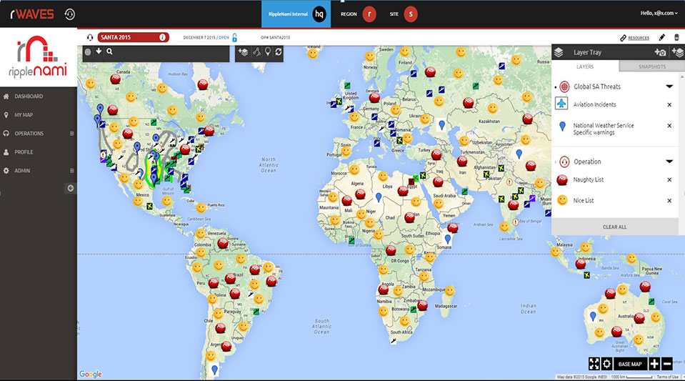
An interesting interactive map has been created by Movoto that allows the user to look at the number of homeless per 100,000 people in each state. But Geographic Information Systems (GIS), community involvement, and app builders are helping gather and utilize data to truly make a difference.

It’s not surprising to note that most of homeless shelter users have goals, both short and long term. Kelly A. Schwend , Maureen Cluskey , and Michael Cordell of Bradley University explored these in a study released early this year titled “Lifestyles and Goals of Male Homeless Shelter Users.” While most participants short term goals are focused on employment, almost all of them had medium to long term goals involving housing.
The questions raised are several. How do we move the homeless from the streets into some kind of housing ladder, and who will assist them? GIS is helping to answer these questions in some of the larger population centers around the country. These programs are merely examples of what can be done elsewhere on a larger or smaller scale.
San Francisco
Over 10 years ago, then mayor of San Francisco Garvin Newsom promised that the worst of the homeless problem in one of the richest cities in the world would be gone. Ten years later, the city has moved nearly 20,000 homeless of the streets, but this hasn’t made a dent in the population. It seems that when one individual is helped, another takes their place.

San Francisco Open Data contains information on the homeless population, counted by supervisory district. Taking this data, Bill Levay then overlays a San Francisco neighborhood shapefile. This not only shows where the homeless populations are concentrated, but by also adding in mapped locations of public and affordable housing locations, reveals if the resources are located near those in need. You can view the interactive map above here.)

For instance, we can see on the map showing the intersection of this data that while a large portion of the homeless population is located near downtown and the South of Market area where there are only a few scattered public housing locations, there is much more public housing clustered together in Chinatown. While this issue has yet to be corrected, this information can be used to inform future decisions when locating resources.
Los Angeles
San Francisco is not the only populous city dealing with homelessness. Los Angeles is dealing with one of the largest homeless populations in the nation. A biennial survey taken in January, said to be the most rigorous and accurate so far according to City Labs, reveals 44,359 people sleeping on the streets, in their cars, and in shelters.

A map created by the Los Angeles Times shows where this population ends up at night. Efforts are spotty at best, although the County’s Housing for Health program wants to have 10,000 permanent housing units created by 2018. Although Mayor Eric Garcetti says ending homelessness is a primary goal, and calls for funding for affordable housing, the problem continues to grow.
It is hoped that mapping the concentration of the population to help resource teams know what locations to target, the revision of laws prohibiting sleeping in public, and discouraging police raids on homeless encampments will help.
Baltimore
Baltimore’s homeless population is smaller than that of Los Angeles, but still significant. The city is using both mapping and a survey taken every two years to locate the homeless and target resources.
They’ve added another weapon to their arsenal, the Homeless Management Information System, (HMIS) spearheaded by the group The Journey Home and the Mayor’s Office for Health. Using this data, and a new web survey form, the city has obtained a more accurate picture of the homeless population, its location, and the resources still needed.
The survey, called the Point in Time (PIT), this year counted 2,796 homeless, 88% of whom were housed in shelters. The survey also looked at Housing Information Count (HIC). The study showed some progress and some setbacks, and revealed growth in the category of unaccompanied youth.

The map above shows the population, and the location of resources all within a one and a half mile radius. The program not only uses mapping, but employs other technology to attempt to create long term, sustainable, and creative solutions to the city’s homeless issues.
New York City
Perhaps the most innovative mapping program in the country involves several apps being used in New York City. Launched in early August the new app called NYC Map the Homeless lets users take a picture of the homeless which is tied to their location, and use hashtags like #man or #sleeping to categorize individuals. They can even choose #violent to let authorities know about individuals perceived to be dangerous.
Photo Credit: NYC Map the Homeless
The idea, according to the developer, is to “gather as much data as possible to make sense of the homeless issues we’re seeing.”
He’s far from the first to try to use technology to address the increasing homeless issues in New York City, Homeless Helper, Feed it Forward, and WeShelter. WeShelter, provides direct assistance to the homeless, and wants create a behavior change from doing nothing to doing something, even if the user is not sure what to do.
The app lets users donate money to the homeless at the tap of a button, and also send location information to WeShelter, which helps them send outreach teams to areas with the most need.
Unlike Map the Homeless, WeShelter does not allow users to take pictures in the interest of privacy. it also keeps the location data it gathers closer to the vest, only making it available to homeless outreach groups.
Regardless of the location or the methodology, it is clear that mapping the locations of the homeless population and the resources available to them is a step in the right direction. GIS plays a large role in aiding social action.
Want to be a part of the solution? The Journey Home has some answers, but you can also get involved in your own community using the skills you have to aid in the eradication of homelessness. As WeShelter states, it’s all about a change in behavior from doing nothing to doing something.


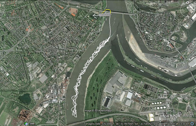
![Figure 3. Layout of the first trajectory [DOY: 2014/126], zoom-in on bottom. (Photo: Google Earth)](https://stage.globalpositioningnews.com/wp-content/uploads/2015/12/Figure-4-W.jpg)
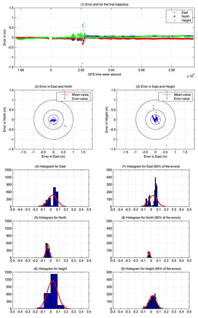
![Figure 4. Satellite residuals for the first trajectory [DOY: 2014/126].](https://stage.globalpositioningnews.com/wp-content/uploads/2015/12/Figure-5-W.jpg)
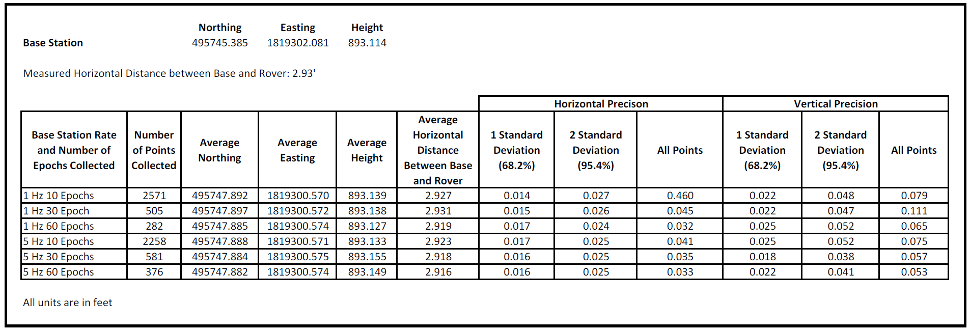
![Table 1. Statistical results of the first trajectory [DOY: 126/2014].](https://stage.globalpositioningnews.com/wp-content/uploads/2015/12/Table1.jpg)
![Figure 6. Layout of the second trajectory [DOY: 127/2014]. (Photo: Google Earth)](https://stage.globalpositioningnews.com/wp-content/uploads/2015/12/Figure-7-W.jpg)
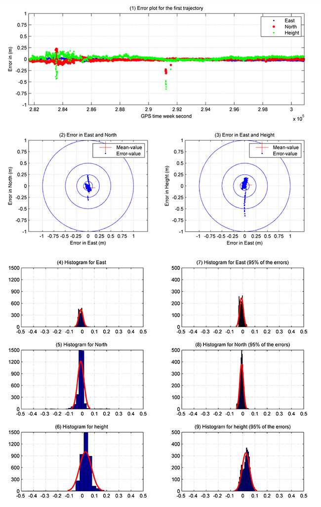
![Figure 7. Satellite residuals for the second trajectory [DOY: 127/2014].](https://stage.globalpositioningnews.com/wp-content/uploads/2015/12/Figure-8-W1.jpg)
![Table 2. Statistical results of the second trajectory [DOY: 127/2014].](https://stage.globalpositioningnews.com/wp-content/uploads/2015/12/Table2.jpg)