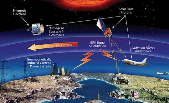
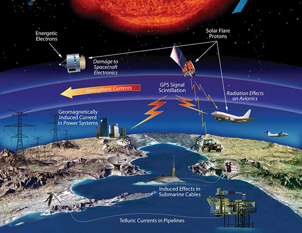
The effects of space weather on critical Earth systems. (Image: NASA)
The United States Congress has passed bipartisan legislation to address how the government deals with threats posed by emissions from the Sun to critical infrastructure such as GPS.
The Promoting Research and Observations of Space Weather to Improve the Forecasting of Tomorrow (PROSWIFT) Act S.881 now awaits signature by the president.
The bill sets forth provisions to improve the ability of the United States to forecast space weather events and mitigate its effects.
It provides statutory authority for the National Science and Technology Council’s Space Weather Operations, Research, and Mitigation Working Group, which coordinates executive branch efforts to understand, prepare, coordinate, and plan for space weather.
The bill directs the Office of Science and Technology Policy, National Oceanic and Atmospheric Administration (NOAA), National Science Foundation, Air Force, Navy, National Aeronautics and Space Administration (NASA), National Security Council, and Federal Aviation Administration (FAA) to carry out specified space weather activities.
The legislation
assigns roles and responsibilities to agencies involved in space weather research and forecasting
ensures agency coordination to better predict severe space weather events and mitigate impacts
calls for coordination between the government and the non-governmental space weather community including academia, the commercial sector and international partners.
Senators Gary Peters (D-MI) and Cory Gardner (R-CO) introduced the first version of the bill in 2016 and a successor passed the Senate in 2017. Reps. Ed Perlmutter (D-CO) and Mo Brooks (R-AL) shepherded it through the House, which passed it Sept. 16.
As technology evolves, the Civil Air Patrol will continue to be a platform for implementing new technologies to secure the country in times of crisis.
The strength of this country isn’t in buildings of brick and steel. It’s in the hearts of those who have sworn to fight for its freedom! —Captain America
Eyes of the Home Skies, World War II-era poster of Civil Air Patrol. (Image: CAP)
If you are someone who likes aviation, GIS and emerging technologies like artificial intelligence and computer vision, and you want to fulfill a greater sense of purpose, the perfect time is now.
The Flying Minute Men, so called by Robert Neprud in the 1948 Story of the Civil Air Patrol (CAP), serve on the frontlines of national threats and disasters. They are the air wing for first responders.
CAP works with many government organizations including the Federal Emergency Management Administration (FEMA), The National Geospatial-Intelligence Agency (NGA), the National Oceanic Atmospheric Administration (NOAA), the Army Corps of Engineers, the National Guard, and many others.
CAP works with non-government organizations too, such as the United States Geospatial Intelligence Foundation (USGIF), the GIS Corps, the National Alliance for Public Safety GIS (NAPSG), and the Red Cross.
CAP also works with youth teaching valuable skills in leadership, community service, STEM and aviation. It has a proud heritage originating in World War II.
In the final days of 1941, the world was in flames. Dark shadows lurked in the waters off American shores. German U-boats attacked ships along the coast. The newly established Office of Civilian Defense understood the importance of aviation for stopping the U-boat threat but lacked the military resources. On Monday, December 1, 1941, six days before the attack on Pearl Harbor, Administrative Order 9 was signed creating the Civil Air Patrol, but there would be no celebration. The threat was all too real. The Battle of the Atlantic had begun. Within a few months Germany sank over 230 ships in U.S. waters. American shores were on fire.
A list of known shipwrecks and their locations in U.S. waters can be downloaded from NOAA’s Coastal Survey website. It is not a complete or a clean dataset so some wrangling will be required. A shortcut is using the shipwreck layer in Google Earth. Along the Atlantic Coast, Gulf of Mexico, and Caribbean Sea there are multiple sunken German U-boats. Most notably are U-85, the first U-Boat sunk by the U.S. Navy in WWII, less than 20 miles off of Nag’s Head, North Carolina (35.885, -75.2829); and U-853, the last one to be sunk in WWII 10 miles off the coast of Rhode Island less than 24 hours before Germany’s surrender (41.2268, -71.4187).
The American tanker SS Harry F. Sinclair burns south of Cape Lookout North Carolina, torpedoed by U-203 on April 11, 1942. (Photo: U.S. Naval History and Heritage Command)
During the War, the Civil Air Patrol flew 5,684 aerial escorts for shipping convoys keeping the sea lanes safe and enabling supplies to get to Europe and North Africa. Shortly after the war, on July 1, 1946, President Truman recognized the valuable contribution made by the Civil Air Patrol making them permanent, but once again there was no celebration. On the same day, responding to overwhelming public attention, TIME published “COSMOCLAST EINSTEIN: All matter is speed and flame.” Radios around the world tuned-in as the clock counted down to zero hour. The first post-war atomic bomb was detonated at 22:00 Greenwich Mean Time (5:00 PM Eastern) in Bikini Lagoon (11°36’00” N 165°29’00” E) over a ghost fleet of ninety-five ships in the middle of the Pacific. History’s long shadow fell over the moment. The applause of a grateful nation for the Flying Minute Men was silence.
It is the mark of real heroes, duty is the highest honor, the rewards are personal having the courage to stand in the face of danger and clasp the hand of Victory. It is valor not fame that makes heroes of normal men and women. The Civil Air Patrol rarely makes the front page, but it supports many of the nation’s most significant events.
Photo of Ground Zero taken on September 12, 2001 by Civil Air Patrol. (Photo: CAP)
The first photographs of Ground Zero released to the public the day after September 11, 2001, were taken by the Civil Air Patrol. With the creation of the Department of Homeland Security in 2002 the Civil Air Patrol took on a much larger role in homeland security. CAP serves a unique purpose flying a multitude of missions because aircraft can fly for extended periods at optimum altitudes to get the best resolution. CAP imagery is often the most currently available and of the highest quality after an event. The Civil Air Patrol aircraft can carry interchangeable sensor arrays, such as thermal cameras, synthetic aperture radars, lidar, communications equipment, and more. Imagery collected by the Civil Air Patrol is publicly available on the CAP GIS Portal.
In 2017, FEMA hosted a Disaster Crowdsourcing Exchange laying a foundation for working with the Civil Air Patrol to push the imagery out to various crowdsourcing channels. The Red Cross Humanitarian OpenStreetMaps Team (HOT) used it to map road networks. Crowdsourced imagery analysts used it for feature extraction and damage assessments. In 2018, this effort was developed further using Hurricane Michael imagery of Panama City, Florida, for creating artificial intelligence algorithms to identify and extract features.
The Civil Air Patrol captures imagery with the WaldoAir XCAM Ultra 50 by flying in overlapping circles as the aircraft sweeps over a disaster area. The overlapping images allow the system to create high-resolution 3D point clouds. The spatial intelligence algorithms employed with post flight processing conducted by Skyline and GeoX can automate feature extraction of buildings, vehicles, bridges, roads, cell towers, and other structures, and identify structures as destroyed, damaged, or undamaged. The system can begin damage assessments almost immediately. The process used to take several weeks with an enormous cadre of specialists and resources and now it can finish in a few days or less with a handful of specialized staff.
I had the privilege of speaking with the Director of Operations for the Civil Air Patrol, Mr. John Desmarais, or Moose as his friends know him. He is a 33-year veteran of CAP, has a pilot’s license, a master’s degree from Embry-Riddle Aeronautical University and is married with two children. Moose shared how September 11th, 2001 changed his commitment and understanding of C.A.P.’s role working with and supporting homeland security missions. He shared with me some of the stories above and gave me an in-depth look into CAP’s future.
Screenshot: Civil Air Patrol
Today, the Civil Air Patrol supports important missions. For FEMA CAP does post-event damage assessments after hurricanes, floods, tornadoes, fires, earthquakes, dam bursts, and more. This will be able to get people the assistance they need much faster ultimately saving lives. This year alone, the Civil Air Patrol has saved 91 lives according to the Air Force Rescue Coordination Center. Other examples are providing search & rescue, border protection, homeland security, emergency flight services, remote sensing, humanitarian support, education and training, and Air Force training support to name a few. These initial successes led Christopher Vaughan, the Geographic Information Officer of FEMA, to request the Civil Air Patrol provide GIS support for natural disaster operations. CAP remains very active fulfilling that commitment. Mr. Desmarais said that CAP took close to half a million pictures for the 2018 hurricane season. FEMA hosts all of CAP’s publicly available imagery as part of its GEOPlatform.
Civil Air Patrol Cessna. (Photo: CAP)
GIS has always been a huge part of what the Civil Air Patrol does when looking at it from a basic level of identifying locations, features, and information. Now, GIS is becoming central to the operations of the Civil Air Patrol because it is a force multiplier as in the example above, using spatial intelligence for completing disaster estimates in days instead of weeks with a fraction of the staff. This is powerful and driving the future of CAP towards a more geocentric operation. CAP’s GIS future is in modeling, remote sensing, crowdsourcing, artificial spatial intelligence, and data sharing.
In 2019, the Civil Air Patrol proposed its path forward creating opportunities for its members to gain valuable GIS skills and creating a qualification in GIS Operations. The Civil Air Patrol has recently begun fielding courses with support from its partners to provide training qualifications. Members of CAP can receive the following training courses: GIS for Emergency Managers, GIS Applications for Emergency Management, GIS Specialist and training in HAZUS, a GIS-based hazard analysis tool. This requirement for operations to become geocentric is so great that a call went out for people who are doing GIS work to reach out to the Civil Air Patrol Wing in their local area and consider joining. To find out more get in touch with your local Wing, visit www.GoCivilAirPatrol.com and enter your zip code to find a CAP squadron near you or you can reach out to the CAP National GIS team at [email protected] for more information. The Civil Air Patrol is using GIS more every day for search and rescue operations where CAP members are locating aircraft crash sites using ADS-B and radar data, and locating missing persons using cell phone forensics, and creating situational awareness maps for tracking resources and planning purposes for CAP senior leaders.
The Civil Air Patrol is investing into autonomous aircraft technologies. It has the largest inventory of small unmanned aerial systems (sUAS) for civilian/ public safety use in the nation. The great advantages to CAP for sUAS are their low costs to deploy and their ability to collect close-up, high-resolutions imagery with minimal risk to people. In disaster areas flying low level flights are extremely hazardous to piloted aircraft because wires and cables and other smaller objects that have shifted. The use of sUAS will fly alongside emergency responders and CAP expects to have sUAS available for each of its 150 incident command posts across the country by the end of 2020 with over 1,000 trained operators nationwide.
In the future, the high-resolution 3D imagery point clouds will enable the Civil Air Patrol to provide real-time virtual environments and augmented reality enhanced awareness for humanitarian assistance and disaster relief operations, especially when that imagery is infused with powerful geographic information systems and artificial spatial intelligence algorithms.
In the near term, the Civil Air Patrol will be expanding the number of aircraft it has equipped with FLIR and other high-end sensors and will continue growing its sUAS operations. It will continue its outreach efforts to build working relationships with new partners and bring onboard volunteers interested in supporting GIS and imagery analysis.
As technology evolves, the Civil Air Patrol will continue to be a platform for implementing new technologies to secure the country in times of crisis. The words spoken by Colonel Scott at the First Report to Congress in May 1948 continue to ring true.
“I predict that the Civil Air Patrol will grow immeasurably stronger — it will continue to contribute to the strength and the security of this nation.” —Colonel Scott, First Report to Congress, May 1948
To get the best measurements of Earth’s atmosphere, you sometimes have to leave it. This November, the Sentinel-6 Michael Freilich spacecraft will do just that.
News from the Jet Propulsion Laboratory
When a satellite by the name of Sentinel-6 Michael Freilich launches this November, its primary focus will be to monitor sea-level rise with extreme precision. But an instrument aboard the spacecraft will also provide atmospheric data that will improve weather forecasts, track hurricanes and bolster climate models.
“Our fundamental goal with Sentinel-6 is to measure the oceans, but the more value we can add, the better,” said Josh Willis, the mission’s project scientist at NASA’s Jet Propulsion Laboratory in Southern California. “It’s not every day that we get to launch a satellite, so collecting more useful data about our oceans and atmosphere is a bonus.”
A U.S.-European collaboration, Sentinel-6 Michael Freilich is one of two satellites that compose the Copernicus Sentinel-6/Jason-CS (Continuity of Service) mission. The satellite’s twin, Sentinel-6B, will launch in 2025 to take over for its predecessor. Together, the spacecraft will join TOPEX/Poseidon and the Jason series of satellites, which have been gathering precise sea-level measurements for nearly three decades. Once in orbit, each Sentinel-6 satellite will collect sea-level measurements down to the centimeter for 90% of the world’s oceans.
JPL-developed instrument
Meanwhile, they’ll also peer deep into Earth’s atmosphere with GNSS-RO to collect highly accurate global temperature and humidity information. Developed by JPL, the spacecraft’s GNSS-RO instrument tracks radio signals from navigation satellites to measure the physical properties of Earth’s atmosphere. As a radio signal passes through the atmosphere, it slows, its frequency changes, and its path bends. Called refraction, this effect can be used by scientists to measure minute changes in atmospheric physical properties, such as density, temperature, and moisture content.
The precise global atmospheric measurements made by Sentinel-6 Michael Freilich will complement atmospheric observations by other GNSS-RO instruments already in space. Specifically, the National Oceanic and Atmospheric Administration’s National Weather Service meteorologists will use insights from Sentinel 6’s GNSS-RO to improve weather forecasts.
Also, the GNSS-RO information will provide long-term data that can be used both to monitor how our atmosphere is changing and to refine models used for making projections of future climate. Data from this mission will help track the formation of hurricanes and support models to predict the direction storms may travel. The more data we gather about hurricane formation (and where a storm might make landfall), the better in terms of helping local efforts to mitigate damage and support evacuation plans.
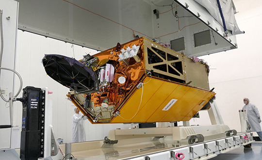
The Sentinel-6 Michael Freilich spacecraft undergoes tests at its manufacturer Airbus in Friedrichshafen, Germany, in 2019. The white GNSS-RO instrument can be seen attached to the upper left portion of the front of the spacecraft. (Photo: Airbus)
A brief history of radio occultation
Radio occultation was first used by NASA’s Mariner 4 mission in 1965 when the spacecraft flew past Mars. As it passed behind the Red Planet from our perspective, scientists on Earth detected slight delays in its radio transmissions as they traveled through atmospheric gases. By measuring these radio signal delays, they were able to gain the first measurements of the Martian atmosphere and discover just how thin it was compared to Earth’s.
By the 1980s, scientists had started to measure the slight delays in radio signals from Earth-orbiting navigation satellites to better understand our planet’s atmosphere. Since then, many radio occultation instruments have been launched; Sentinel-6 Michael Freilich will join the six COSMIC-2 satellites as the most advanced GNSS-RO instruments among them.
“The Sentinel-6 instrument is essentially the same as COSMIC-2’s. Compared to other radio occultation instruments, they have higher measurement precision and greater atmospheric penetration depth,” said Chi Ao, the instrument scientist for GNSS-RO at JPL.
GNSS-RO basics
The GNSS-RO instrument’s receivers track navigation satellite radio signals as they dip below, or rise from, the horizon. They can detect these signals through the vertical extent of the atmosphere — through thick clouds — from the very top and almost all the way to the ground. This is important, because weather phenomena emerge from all layers of the atmosphere, not just from near Earth’s surface where we experience their effects.
“Tiny changes in the radio signal can be measured by the instrument, which relate to the density of the atmosphere,” said Ao. “We can then precisely determine the temperature, pressure, and humidity through the layers of the atmosphere, which give us incredible insights to our planet’s dynamic climate and weather.”
With the help of JPL’s GNSS-RO principal investigator Chi Ao and NOAA’s National Weather Service meteorologist Mark Jackson, this video explains how the GNSS-RO instrument aboard Sentinel-6 Michael Freilich will be used by meteorologists to improve weather forecasting predictions. (Credit: NASA/JPL-Caltech)
But there’s another reason why probing the entire vertical profile of the atmosphere from orbit is so important: accuracy. Meteorologists typically gather information from a variety of sources – from weather balloons to instruments aboard aircraft. But sometimes scientists need to compensate for biases in the data. For example, air temperature readings from a thermometer on an airplane can be skewed by heat radiating from parts of the aircraft.
GNSS-RO data is different. The instrument collects navigation satellite signals at the top of the atmosphere, in what is close to a vacuum. Although there are sources of error in every scientific measurement, at that altitude, there’s no refraction of the signal, which means there’s an almost bias-free baseline to which atmospheric measurements can be compared in order to minimize noise in data collection.
And as one of the most advanced GNSS radio occultation instruments in orbit, said Ao, it will also be one of the most accurate atmospheric thermometers in space.
More on the mission
Copernicus Sentinel-6/Jason-CS is being jointly developed by the European Space Agency (ESA), the European Organisation for the Exploitation of Meteorological Satellites (EUMETSAT), NASA, and the National Oceanic and Atmospheric Administration (NOAA), with funding support from the European Commission and support from France’s National Centre for Space Studies (CNES).
The first Sentinel-6/Jason-CS satellite that will launch was named after the former director of NASA’s Earth Science Division, Michael Freilich. It will follow the most recent U.S.-European sea-level observation satellite, Jason-3, which launched in 2016 and is currently providing data.
NASA’s contributions to the Sentinel-6/Jason-CS mission are three science instruments for each of the two Sentinel-6 satellites: the Advanced Microwave Radiometer, the GNSS-RO, and the Laser Retroreflector Array. NASA is also contributing launch services, ground systems supporting operation of the NASA science instruments, the science data processors for two of these instruments, and support for the international Ocean Surface Topography Science Team.
There are many ways to navigate. For most applications, none surpass the accuracy, affordability and convenience of satellite navigation.
However, given the threats to GNSS from spoofing and jamming, and the possibility that GNSS satellites could be destroyed accidentally by space debris or intentionally during a war, the search is on for alternative sources of positioning, navigation and timing (PNT) data.
Potential alternative PNT (APNT) approaches include computer vision, terrain contour matching (TERCOM, which was used to guide cruise missiles in the 1970s and 1980s), and using magnetic anomalies (MAGNAV).
Diverse animals — such as sea turtles, spiny lobsters, and birds — use magnetoreception for orientation and navigation. However, while animals likely perform wayfinding using the direction of the magnetic field, similarly to how humans use a compass, high-resolution maps used in conjunction with atomic instruments enable us to perform absolute positioning to tens of meters, explained Major Aaron Canciani.
Canciani, an assistant professor of electrical engineering at the Air Force Institute of Technology, has been designing algorithms for MAGNAV flight testing for several years.
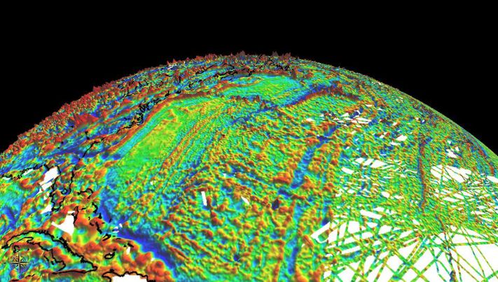
Earth’s crustal magnetic field varies from location to location as much as topographic features do and, like them, it changes very little over time. However, unlike topographic features, which only occur on the third of the planet’s surface covered by land, magnetic variations also occur on the oceans. This makes them potentially very useful as landmarks to the Navy and Air Force. Magnetic variations have the additional benefit that they cannot be jammed or spoofed.
NOAA’s EMAG2 World Digital Magnetic Anomaly Map. (Image: NOAA National Geophysical Data Center)
Just like other features of Earth, magnetic fields can be mapped, using scalar magnetometer sensors to measure their strength and direction. In fact, government agencies and mining companies have been making these maps for many decades, for geological exploration and other purposes, though mostly on land.
Conversely, these maps can be used to navigate by comparing the data from magnetometers to the map, just like cruise missiles used to use on-board radar altimeters to match the contours of the land beneath them to contour lines on a digital map and navigators on vessels in shallow waters compare the depths reported by their fathometers to those marked on a chart.
Before this approach to navigation can be widely implemented, however, magnetic maps need to greatly improve in coverage and quality. In addition to magnetic maps and sensors, MAGNAV also requires sophisticated algorithms and careful calibration, to do such things as subtract errors from space weather and the local magnetic field of the aircraft or ship.
The greater the platform’s speed, the greater MAGNAV’s accuracy, because the magnetometers can collect more varying magnetic information per unit of time of INS drift, Canciani explains. On a platform moving fast and at low altitudes, MAGNAV could achieve 10-meter accuracy. In less ideal conditions and relying on lower quality magnetic maps, the accuracy could be as low as one kilometer — which is sufficient for many missions, such as navigating ships at sea.
Off-the-shelf scalar magnetometers about the size of a quarter have already been flight tested. Corporations, the military and civilian government agencies such as NOAA, NASA and NGA already have suitable magnetic maps, though they need to be improved and expanded, particularly at sea. This would require gathering new data using calibrated sensors on airplanes, ships and submarines.
Could magnetic sensors be installed on thousands of aircraft, land vehicles and sea vessels to collect magnetic data during their routine operations? “With proper calibration, yes, but it should not be downplayed how difficult it is to get 1 nanoTesla measurements on a platform,” Canciani said. “Mapping and navigation are inverse problems so any platform that has been calibrated well enough to navigate could, in turn, also be used for mapping.”
However, he points out, the task is much more complicated than just putting a magnetometer on a platform. “Getting clean data on complex platforms remains the largest challenge for magnetic navigation,” Canciani said, “although we are making excellent progress with projects like the Air Force Accelerated AI program with MIT and Lincoln Lab. In this project we are using state of the art scientific machine learning approaches to calibrate complex magnetic fields on operational platforms. Without excellent calibration algorithms the only sure-fire way to get clean magnetic data is putting a sensor out on a boom or wing-tip, which might not be practical for all use cases.”
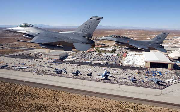
Two F-16 Fighting Falcons fly over Edwards AFB during a 2009 air show. (Photo: U.S. Air Force/Chad Bellay)
Canciani admits that MAGNAV is often met with skepticism but hopes that realistic testing on realistic platforms will lead to more interest and funding for this approach.
While some such testing has already been performed using private survey aircraft, a much more important test will take place in September, when F-16s from the Air Force Test Pilots School will fly MAGNAV sensors and software over a test range next to Edwards Air Force Base in Nevada.
On June 26, the U.S. National Oceanic and Atmospheric Administration (NOAA) released the summary of the results of Commercial Weather Data Pilot (CWDP) Round 2. View the summary here.
In Round 2, NOAA evaluated GNSS radio occultation data from two U.S. commercial space companies: GeoOptics and Spire. NOAA concludes that, based on the results of CWDP Round 2, the commercial sector is able to provide radio occultation data that can support NOAA’s operational products and services.
“As a result, NOAA is proceeding with plans to acquire commercial RO data for operational use,” the summary states.
According to GeoOptics, the report highlights the unique qualities of its commercial GNSS-RO data and its ability to improve weather and space weather forecasts around the world.
“As today’s report demonstrates, commercial satellite data will enable NOAA to make significant improvements in forecasting worldwide within the consistent budget limitations under which it operates,” said GeoOptics CEO Conrad Lautenbacher.
NOAA anticipates release of a request for proposals soon for operational purchase of commercial radio occultation data, continuing an acquisition process that began in April with NOAA’s release of a draft Statement of Work.
NOAA has requested $15 million in FY 2021 to support Commercial Data Purchase. The FY 2021 Budget also requests $8 million for CWDP to investigate new commercial technologies beyond radio occultation.
By moving into this next phase of engagement with U.S. industry, NOAA is leveraging commercial space sector capabilities to support its operational products and services and to continue to improve its weather forecasting capabilities. NOAA plans to implement additional rounds of the CWDP to evaluate commercial capabilities beyond radio occultation data for potential operational use.
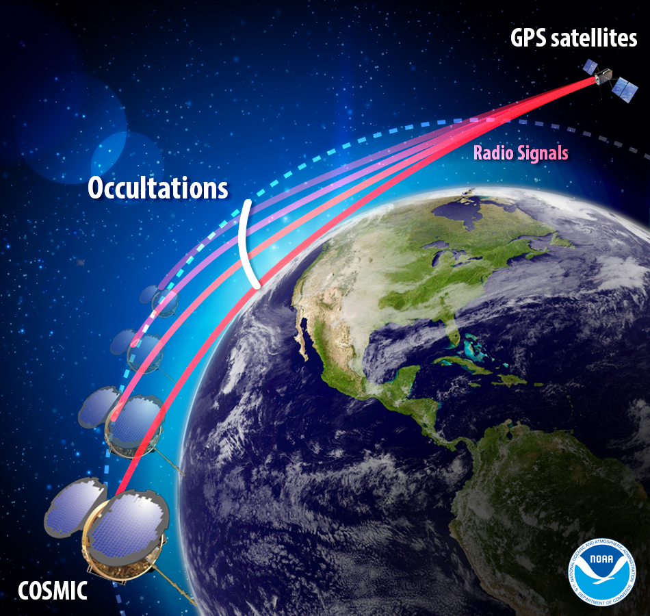
The COSMIC-1 program ended on May 1, when the last of six tiny satellites were decommissioned. The satellites were launched 14 years ago, and outlived their planned lifespan by 12 years.
COSMIC — the Constellation Observing System for Meteorology, Ionosphere and Climate (COSMIC) mission — uses GPS signals to provide a wealth of accurate atmospheric data and improve weather forecasts, according to Laura Snider, University Corporation for Atmospheric Research (UCAR), which ran the COSMIC program.
Meanwhile, the COSMIC-2 program (FORMOSAT-7 in Taiwan) continues. Its six satellites were launched on June 25, 2019, into low-inclination orbits. The mission was launched by NOAA as the agency’s first operational GNSS radio occultation mission.
COSMIC-1 demonstrated the value of GNSS radio occultation (GNSS-RO) to derive vertical atmospheric profiles of temperature, humidity and pressure by measuring the degree to which GPS signals bend as they travel through Earth’s atmosphere.
Weather centers used the high-quality, accurate data to improve forecasts; the data was also used by researchers.
“Throughout its lifetime, COSMIC-1 made an astounding 7 million vertical atmospheric profiles available to the operational forecast centers and research community,” writes Snider. “These data demonstrably boosted forecast accuracy and were referenced in more than 550 peer-reviewed scientific publications. In all, more than 5,000 users from over 100 countries have accessed COSMIC data.
COSMIC-1 was primarily funded by the National Space Organization in Taiwan, where the mission is called FORMOSAT-3. The leading U.S. sponsor on the project was the National Science Foundation. Other U.S. partners included NASA, the National Oceanic and Atmospheric Administration (NOAA), the Air Force and the Office of Naval Research.
UCAR also led the GPS/MET GPS radio occultation mission in the mid-1990s.
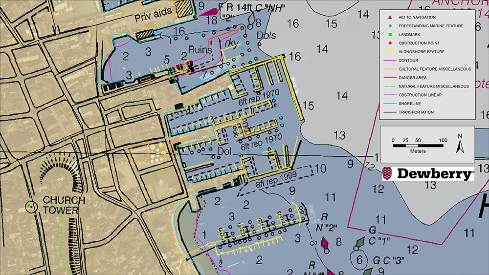
Existing NOAA nautical chart of Nantucket Harbor, Mass., overlaid with revised shoreline features collected by Dewberry. Image courtesy of Dewberry. (Image: Dewberry/NOAA)
Dewberry has been selected by the National Oceanic and Atmospheric Administration (NOAA) for the agency’s Shoreline Mapping Services contract. The five-year, indefinite delivery/indefinite quantity (IDIQ) contract has a ceiling of $40 million and will enable Dewberry and its partners to work with NOAA’s National Geodetic Survey to develop new technologies and initiatives to protect the nation’s coasts.
This is Dewberry’s second consecutive shoreline mapping services contract for NOAA. Over the past five years, the firm completed 30 task orders across the nation, including research studies to analyze bathymetric point tracing, derive bathymetry from satellite data, and apply INSAR data to analyze subsidence.
Task orders also included shoreline mapping in Alaska; creating topobathymetric lidar and shoreline products from NOAA-acquired data in Connecticut, Puerto Rico, the Chesapeake Bay, Florida and Maryland; acquiring and processing topobathymetric lidar data in Puerto Rico, the U.S. Virgin Islands, Texas and Massachusetts; and developing topobathymetric elevation and shoreline mapping datasets along the Atlantic seaboard from Myrtle Beach, South Carolina, to Long Island, New York.
“We are excited to continue to support and partner with NOAA to update the national shoreline, nautical charts, and provide high-resolution topography and bathymetric data to enhance the National Coastal Mapping Program,” said Amar Nayegandhi, CP, CMS, GISP, Dewberry’s senior vice president and senior project manager for the contract. “We always strive to find the most appropriate technology and solutions for NOAA and its numerous stakeholders. The task orders we received under the previous contract are a testament to the breadth of geospatial, scientific, and technology services we offer to NOAA.”
Dewberry also conducted special initiatives such as supporting the GRAV-D program to assist in developing the new gravimetric geoid model for 2022 and the 3D Nation Requirements and Benefits Study in collaboration with NOAA and the U.S. Geological Survey (USGS).
The 3D Nation Study documents topographic, coastal, and bathymetric 3D elevation data requirements and benefits across a multitude of geographies, helping to establish a baseline understanding of national business uses, needs and associated benefits for 3D elevation data.
The agreement will enable AER to process satellite data for commercial companies that sell their Earth observation data products to government agencies and other organizations that provide customized environmental information to a range of clients.
Under the agreement, AER will adapt UCAR’s SatDAACâ software system to process observations from satellites using GNSS radio occultation to observe the atmosphere. Those observations can lead to significantly improved weather forecasts.
From basic research to industry
GNSS radio occultation measures the extent to which the radio signals from GNSS transmitter satellites (including GPS satellites) bend as they propagate through denser regions of the atmosphere.
The measurements can be further processed into information about temperature, pressure, and humidity in the lower atmosphere as well as the electron density in the ionosphere. The technique provides considerable accurate knowledge about a large volume of the atmosphere from near-Earth orbit down to the surface.
Image: NOAA
NASA’s Jet Propulsion Laboratory was first to use radio occultation to profile the atmospheres of Mars, Venus, and the outer planets starting in the 1960s. UCAR, in collaboration with JPL, pioneered the GNSS radio occultation observing technique for Earth’s atmosphere, building on basic research with funding from the National Science Foundation.
In 2006, UCAR began producing the first operational GNSS radio occultation data from a specialized constellation of small satellites known as the Constellation Observing System for Meteorology, Ionosphere, and Climate (COSMIC). The observations from COSMIC led to improved predictions of tropical cyclones and other storms as well as information about space weather and global climate.
A second constellation of small satellites, known as COSMIC-2, was launched in June 2019. It will provide twice as many soundings of the atmosphere with higher quality than COSMIC.
More GNSS-RO satellites coming
Now that the technology has been successfully demonstrated, additional satellites with GNSS radio occultation technology are being launched.
“This technology has moved quickly from being a research concept to providing vital information to forecasters,” said Ying-Hwa “Bill” Kuo. “The original investment in basic research is generating substantial benefits for society.”
Lead GNSS radio occultation researcher at AER Stephen Leroy said, “Earth radio occultation has a nearly 30-year history and has been a revolutionary force in numerical weather prediction and climate science in that time; and now with the commercialization of RO [radio occultation] data, we are looking forward to an explosion in RO data volume. I am really excited that we are performing the operational processing of this new data stream and expanding its scope and utility.”
The UCAR-AER agreement will likely lead to further advances in GNSS radio occultation technology, according to Bill Schreiner, director of the UCAR COSMIC Program.
“By transferring technology to the private sector, AER can take it to the next level in terms of distributing the data and finding new applications that help society,” he said. “This agreement will leverage SatDAAC’s advanced capabilities to develop new products for use by the environmental observing and prediction communities and will help us continue to innovate.”
At least three commercial enterprises are currently developing and deploying nanosatellites and microsatellites that perform GNSS radio occultation — Spire, GeoOptics and PlanetiQ — as well as several international space agencies.
AER works with governments and businesses worldwide to advance understanding of climate- and weather-related risks. The company develops analytical tools to help measure and observe the properties of the environment and translate those measurements into actionable information.
UCAR is a nonprofit consortium of 120 colleges and universities focused on research and training in the atmospheric and related sciences.
The months-long wildfires raging in Australia have killed at least 25 people. Millions — possibly 1 billion — animals have died. More than 2,000 houses have been destroyed. Around 150 fires are still burning in New South Wales and Queensland, with hot and dry conditions accompanied by strong winds fueling to the fires’ spread.
With this conflagration rocking the continent down under, satellite imagery has become important to understanding the scope of the disaster. Here are some of the recent captures.
As seen from the ISS
“Talking to my crew mates, we realized that none of us had ever seen fires at such terrifying scale,” European Space Agency astronaut Luca Parmitano tweeted on Monday, sharing photos taken from the International Space Station.
The astronaut posted images showing what he described as “an immense ash cloud” captured at the time the ISS was flying toward sunset.
An immense ash cloud covers Australia as we fly toward the sunset.
Another social media image, shared widely, was interpreted as a map showing the live extent of fire spread, with large sections of the populous eastern coastline molten red. Because of widespread misinterpretation, the original poster then explained that the image was a 3D visualization and not a photograph of Australia, and showed some areas where fires have been extinguished.
NASA and the U.S. Geological Survey’s Landsat 8 satellite imagery from Jan. 9 shows Kangaroo Island, home to nature reserves. The images were taken using the Operational Land Imager (OLI) on Landsat 8. Using natural-color observations, the images show burned land and thick smoke covering the island, of which at least 156,000 hectares have burned.
Photo: NASA/USGS
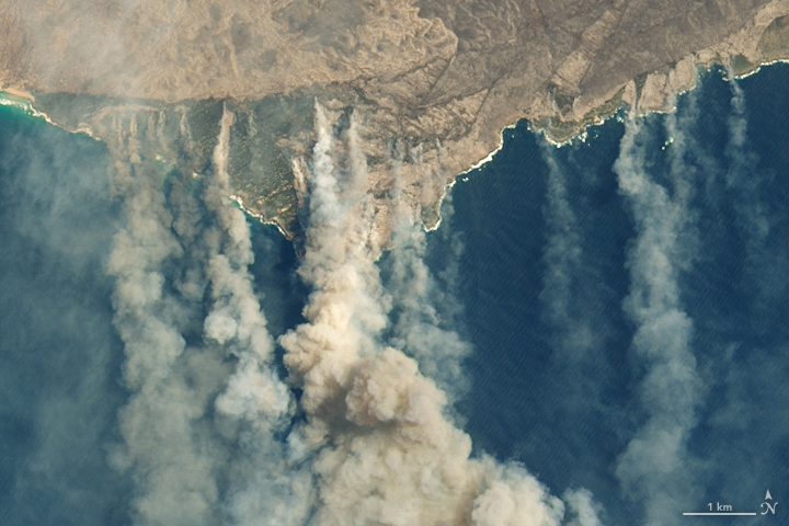
The U.S. National Oceanic and Atmospheric Administration (NOAA) satellites are also capturing images, including the resulting plumes of smoke.
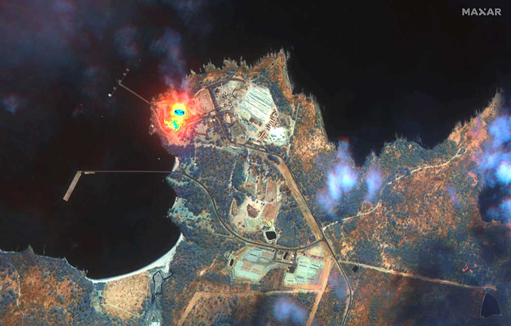
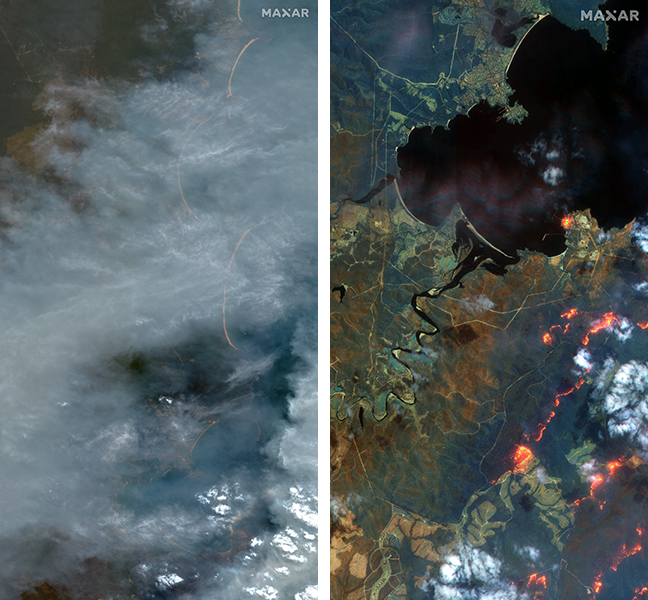
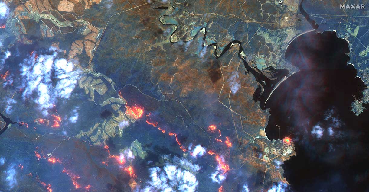
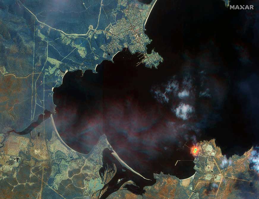
Maxar collected satellite imagery Jan. 12 of the wildfires in New South Wales (NSW). The imagery shown below focuses on the area near the town of Eden, and demonstrates the value of the shortwave infrared (SWIR) sensor.
In an image taken with Maxar’s normal RGB color imagery, the smoky air prevents a clear view of the fires and the hot spots. With Maxar’s WorldView-3 satellite, however, the team is able to penetrate through the smoke using its SWIR sensor for a detailed look at the fire lines and burned vegetation.
With SWIR imagery, burning areas are apparent and show up in a glowing orange-red. Healthy vegetation shows up in shades of blue, and burned vegetation appears in shades of brown.
Satellite Photo: :ESA
Copernicus Sentinel-3 imagery
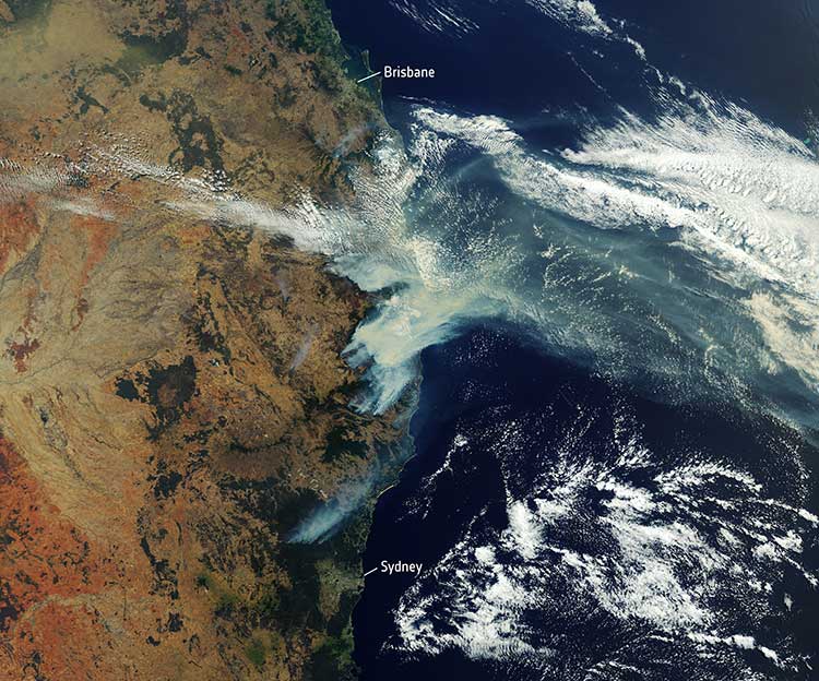
Europe’s Copernicus Sentinel-3 mission has captured the multiple bushfires burning across Australia’s east coast.
In the above image, captured on Nov. 12, 2019, at 23:15 UTC (Nov. 13, 09:15 local time), the fires burning near the coast are visible. Plumes of smoke can be seen drifting east over the Tasman Sea. Hazardous air quality owing to the smoke haze has reached the cities of Sydney and Brisbane.
Flame retardant was dropped in some of Sydney’s suburbs as bushfires approached the city center, and many residents were evacuated. Firefighters continue to keep the blazes under control.
The Copernicus Emergency Management Service – Mapping was activated to help respond to the fires. The service uses satellite observations to help civil protection authorities and, in cases of disaster, the international humanitarian community, respond to emergencies.
Quantifying and monitoring fires is fundamental for the ongoing study of climate, as they have a significant impact on global atmospheric emissions. Data from the Copernicus Sentinel-3 World Fire Atlas shows that there were almost five times as many wildfires in August 2019 compared to August 2018.
The U.S. House Committee on Science, Space and Technology has approved legislation to coordinate federal government space weather research. Included in the bill is a finding that space weather adversely affects space-based position, navigation and timing (PNT).
‘‘The effects of severe space weatheron the electric power grid, satellites and satellite communications and information, aviationoperations, astronauts living and working in space, and space-based position, navigation, and timing systems could have significant societal, economic, national security and health impacts.”
If passed, the bill would mandate coordination of government space weather forecasting and related operations, with input from academia, international groups and commercial firms affected by space weather.
The Promoting Research and Observations of Space Weather to Improve the Forecasting of Tomorrow (PROSWIFT) Act was introduced in November by Democrat Ed Perlmutter of Colorado and Republican Mo Brooks of Alabama, reports Space News. Similar legislation, the Space Weather Research and Forecasting Act, was approved in April by the Senate Commerce, Science and Transportation Committee.
PROSWIFT calls for the National Science and Technology Council to establish an interagency working group on space weather that includes the National Oceanic and Atmospheric Administration (NOAA), NASA, the National Science Foundation, Defense Department and Interior Department. It directs members of the interagency working group to collaborate with the international community, academia and the commercial space weather sector.
PROSWIFT also tasks NOAA with establishing a space weather advisory group with members representing academia, the commercial space weather sector and space weather data customers.
Traditional tide gauges are in contact with the water surface and as a result are susceptible to measurement error and damage during extreme weather. An alternative approach is the use of GNSS reflectometry. We learn how this innovative use of satellite navigation signals works in this month’s Innovation column.
Innovation Insights with Richard Langley
Seawater level is conventionally monitored by tide gauges that measure the vertical distance of the water surface from a point on the ground. As the tide gauges provide seamless and highly accurate measurements, many countries operate a tide-gauge network to monitor sea-level changes and to assess flood risk. For example, the National Oceanic and Atmospheric Administration (NOAA) operates a permanent observing system, the National Water Level Observation Network (NWLON), with more than 400 gauges throughout the United States.
However, some challenges of tide gauges can be identified. Firstly, tide-gauge measurements require direct contact with the water, which causes limitations in installing and maintaining the equipment. The equipment requiring direct sensing is highly vulnerable to coastal hazards, such as coastal flooding and tsunamis, resulting in potential measurement errors or even equipment destruction during severe natural events.
Furthermore, tide gauges require maintenance on a regular basis, which is expensive because it requires the use of divers. This greatly limits the operation of tide gauges, especially in extreme environments such as in the Arctic. Alaska, for example, has significant gaps in its available spatially-varying tidal information. However, in the Arctic, it is also very important to constantly and closely monitor the long- and short-term variation of water levels because this area has a significant impact on global climate and ecosystems. Consequently, more support is needed for sea-level monitoring and coastal mapping in this region.
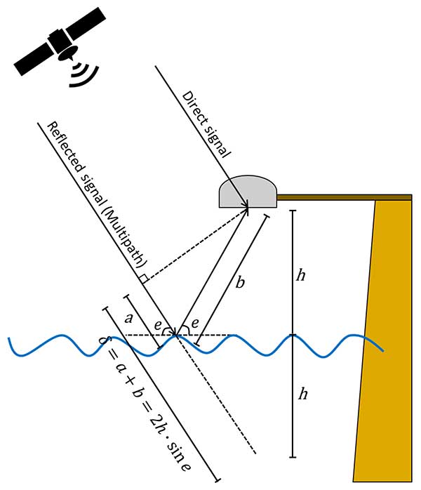
GNSS can serve as an alternative approach for water-level monitoring. GNSS satellites continuously transmit radio signals and ground-based, space-based, and airborne receivers access the signals regardless of weather conditions. Some of the received signals are reflected from obstacles or surfaces near the antenna, a phenomenon referred to as multipath (see FIGURE 1).
FIGURE 1. Schematic drawing of the GNSS-based tide gauge. (Image: Authors)
Multipath tends to be regarded as one of the major error sources for GNSS positioning where it causes unexpected phase delays when compared to the direct signal. Consequently, various procedures have been developed to mitigate the multipath effect. However, the GNSS signals reflected from the Earth’s surface contain information about the geophysical properties of the reflecting surface. The use of these signals is known as GNSS reflectometry (GNSS-R). GNSS-R allows us to monitor the temporal variation of water levels by calculating phase delays of GNSS signals reflected from the water surface. A GNSS-R-based tide gauge does not require direct contact with the water because it measures the water levels based on a remote-sensing technique. Thus, a GNSS-R-based tide gauge can be effectively applied to water-level monitoring.
However, several challenges exist in processing GNSS signals observed at high latitudes compared to mid-latitudes. Not only do we have to contend with extreme weather conditions and limited infrastructure availability, but also with problematic satellite geometry and ionospheric effects on the GNSS signals. To overcome these limitations in the use of GNSS-R in the Arctic, we introduce enhanced algorithms to improve the temporal and spatial resolutions of GNSS-R sea-level measurements.
Our approach includes an enhanced spectrum analysis based on multi-frequency signals and statistical reliability verification. Moreover, we include the signals transmitted by the Galileo constellation in addition to GPS to improve the quantity and the quality of GNSS observations in the Arctic. We have tested the proposed method with an experiment in Alaska and validated the results with nearby tide gauges. The experimental results clearly show the feasibility of employing GNSS-R-based tide gauges in the Arctic.
GNSS-R-BASED WATER-LEVEL MONITORING
Martin-Neria first introduced a method of monitoring sea level using the GNSS-R technique in 1993. Thereafter, many studies have been conducted to apply GNSS-R to water level estimation. Anderson proposed a method to estimate sea level using the interference pattern caused by the direct and reflected GNSS signals, which relies on the fact that the spacing between peaks in the interference pattern is almost entirely dependent on the height of the antenna above the reflecting surface.
The phase difference in the GNSS receiver between the direct and the reflected satellite signals varies while the geometry of a GNSS satellite changes (see Figure 1), generating the interference pattern. The interference pattern is particularly noticeable in signal-to-noise ratio (SNR) data. The reflected signals contribute to the SNR data in the form of oscillations, while the smoothly rising overall arc mostly depends on the signal strength and the antenna gain pattern.
The reflected signals can be isolated from the SNR data by removing the main trend — for example, by polynomial fitting — indicative of the direct signal. The frequency of the remaining dSNR oscillations is constant with respect to the sine of the elevation angle, assuming that the water level does not change during the satellite arc and the reflection surface is horizontal. Consequently, the frequency of the oscillation is linearly proportional to the height of the antenna above the reflecting surface.
The frequency can be derived from the dSNR data by spectral analysis. Among a number of spectral-analysis methods, the Lomb-Scargle periodogram (LSP) is commonly applied since it allows for processing of unevenly sampled data.
Determining the frequency of the oscillations. The antenna height above the water surface is directly calculated from the frequency of the oscillations derived from LSP processing. However, it is difficult to determine the dominant frequency because of the roughness of the water surface, especially in extreme environments such as Arctic regions with high currents and strong winds. In addition, the observed SNR data is easily affected by obstacles near the GNSS antenna. Therefore, it is difficult to distinguish the spectral peak of the signal reflected from the water surface from other additional reflected signals, especially when additional and unexpected reflections occur near the sea surface.
To minimize the erroneous determination of the frequency of the oscillations using dSNR, we can take advantage of the multiple frequencies of modern GNSS signals. In our study, we processed signals from both the GPS and Galileo constellations, with GPS transmitting three carrier signals (L1, L2 and L5) and Galileo transmitting five carrier signals (E1, E5a, E5b, E5ab and E6).
By comparing the spectrum peaks from the multiple signals on different frequencies, one can analyze the dominant peaks across the different frequencies on the same raypath. This algorithm is based on the fact that the multiple frequency signals should detect consistent sea-level heights because they are transmitted along the same raypath during the same period. One of the biggest advantages of this approach is that no additional data or equipment is required to accurately determine the frequency of oscillations of the GNSS signals reflected from the water surface.
Statistical Testing of Retrieved Sea Levels. Reflected signals are not necessarily all from the sea surface. To remove erroneous solutions, we conducted a statistical test. Data including measurement errors and/or some noise can be approximated to the model by the least squares method that determines the model parameters by minimizing the sum of squared residuals. However, this method yields an incorrect result when many outliers deviating from the normal distribution are included in the data set.
This problem can be overcome by applying RANdom SAmple Consensus (RANSAC). RANSAC stochastically estimates the model parameters maximizing consensus, that is, the parameter supported by the largest number of sample data through an iterative process. However, the RANSAC results can act differently each time for the same input data because it is essentially a statistical estimation method using random samples. Therefore, we perform RANSAC with rough constraints primarily to remove outliers significantly out of normal range, then the remaining noise in the data can be excluded by performing secondary fitting using tightly constrained least squares. For the least squares procedure, a series was applied for the fitting model, which represents various motions of the sea surface such as ocean tide loading, as a sum of trigonometric functions.
SEA-LEVEL MONITORING IN ST. MICHAEL
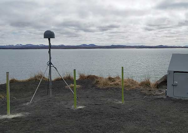
The Plate Boundary Observatory (PBO) network operated by UNAVCO (formerly the University NAVSTAR Consortium) is primarily designed to monitor long-term tectonic and volcanic deformation. However, it can also be used for GNSS-R applications. A new PBO station, AT01, was installed in May 26, 2018, in St. Michael, Alaska, which is designed to be suitable as a GNSS-R-based tide gauge with a clear and wide-open view toward the sea covering from 0° to 230° in azimuth (see FIGURE 2). The equipment at this site consists of a Trimble choke-ring geodetic antenna and a Septentrio PolaRx5 receiver that can receive not only GPS signals but also those of Galileo, with data recorded every 15 seconds.
FIGURE 2. The surrounding area of AT01 in St. Michael, Alaska: south view. (Photo: Authors)
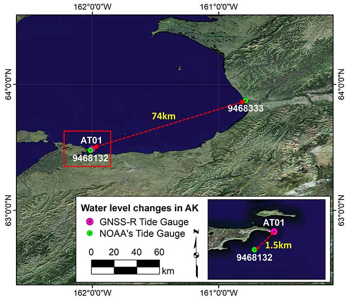
We have used this station to assess our technique using one month of SNR data from June 2018. It should be emphasized that not only GPS but also Galileo signals were processed, and the Center for Orbit Determination in Europe’s Multi-GNSS Experiment final orbit and satellite clock products were used to minimize the satellite orbit error. Additionally, NOAA tide gauge stations (9468132 and 9468333) were used for comparison and verification of the water levels measured from the GNSS-R-based tide gauge (see FIGURE 3).
FIGURE 3. Locations of AT01 and two NOAA tide-gauge stations (9468132 in St. Michael and 9468333 in Unalakleet). The red box represents the zoomed area at the bottom right. (Image: Authors)
The 9468132 tide gauge in St. Michael is the nearest tide gauge at approximately 1.5 kilometers from AT01. However, since it is not operational, NOAA only provides water-level predictions (just high and low tides) based on the harmonic constituents, not the actual measurements. On the other hand, the 9468333 tide gauge in Unalakleet is approximately 74 kilometers away from AT01. This makes it difficult to use the tide gauge as ground truth, but it does provide the actual sea-level measurements including any abnormal daily variations during the observation period. Therefore, we used the water-level predictions and measurements from both stations to validate the GNSS-R-based water-level measurements at AT01.
Determination of Water Level. The GPS and Galileo SNR data were independently analyzed using our in-house software package (written in MATLAB) using the following procedures.
As a preprocessing step, each SNR data series was examined to filter out the signals reflected from other surfaces surrounding the antenna and to isolate the signals that were reflected by the sea surface. Since AT01 PBO station was installed to investigate the feasibility of its use as a GNSS-R-based tide gauge, the most effective azimuth and elevation ranges were given, which are 0° to 230° and 10° to 25°, respectively.
The azimuth and elevation angle ranges were applied, which effectively removed reflected signals from surfaces other than the sea surface. After identifying the SNR data affected by the reflection from the sea surface, the processing windows were dynamically determined by the continuous path and direction (ascending and descending) of the satellites, and the height of the sea surface was estimated using only a portion of the satellite arc contained within each processing window.
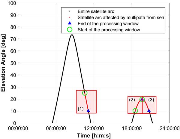
For example, FIGURE 4 shows the processing windows determined for the GPS satellite PRN 1 on June 1, 2018. The red dots in the figure show the parts of the satellite arcs affected by multipath from the sea surface. The data was divided into three processing windows due to the arc discontinuities and satellite path directions. It should be noted that only the processing windows with a data span of 30 minutes or longer were used for water level estimation. This minimum data span duration of 30 minutes was empirically determined by observing the probability of failure of the water -level calculation for shorter spans.
FIGURE 4. An example of the processing window determination for GPS satellite PRN 1 on June 1, 2018. (Image: Authors)
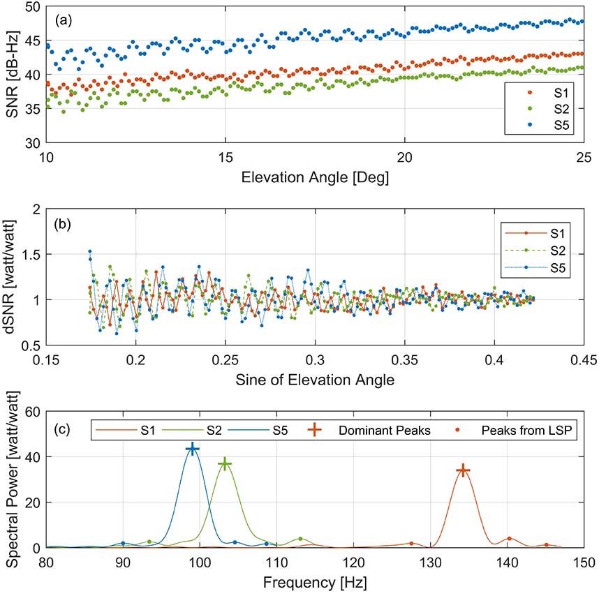
To isolate multipath effects from the SNR observation, we removed the trend in the SNR by a second-order polynomial fitting using only the portion of a satellite arc contained within each window. FIGURE 5 (b) shows the detrended SNR (dSNR) from FIGURE 5 (a), and the impact of the multipath is clearly identified in the form of the oscillation. As discussed earlier, the oscillation frequency is related to the antenna height above the sea surface. Accordingly, the dSNR data was analyzed through an LSP. As shown in FIGURE 5 (c), multiple peaks are founded from the LSP results of each dSNR series, and it is not easy to distinguish the frequency of the reflected signal from the sea level among these peaks.
Since multiple frequency signals from the same satellite must detect the same sea-level height, the final dominant peak was determined by checking the consistency of the resulting heights from each dominant peak among the multi-frequency signals. After that, the dominant frequency was converted to the antenna height above the reflection surface, which was then subtracted from the orthometric height of the antenna (the height above the geoid or, approximately, the height above mean sea level [MSL]) to refer the height of the instantaneous sea surface to MSL.
FIGURE 5. SNR data-analysis procedures with PRN 1 GPS on June 1, 2018: (a) The SNR data affected by the reflection from the sea surface, (b) detrended SNR data through a second-order polynomial, and (c) LSP results and dominant peaks of each frequency. (Image: Authors)
After analyzing all SNR data observed during one day, we carried out the reliability test of the retrieved sea levels to reject erroneous sea-level solutions.
RESULTS AND VALIDATION
The water-level changes from the GNSS-R-based tide gauge at St. Michael were compared to the independently predicted and measured sea levels from the neighboring St. Michael and Unalakleet tide gauges during June 1–30, 2018. Although the tide gauges are considered reliable ground truth, our experimental study must take into account the physical distance between the sites (about 1.5 and 74 kilometers from AT01, respectively) as well as the difference coming from the model versus the actual measurement.
In addition, a vertical offset between the data time series of the GNSS-R-based tide gauge and the standard tide gauges should be considered due to their different datums. Whereas the GNSS-R-derived sea level refers to a geodetic datum — namely the U.S. National Spatial Reference System (NAVD 88) — a standard tide gauge is highly localized with reference to a tidal datum such as local mean sea level. Generally, the difference between the geodetic and tidal datums is provided by NOAA, which allows us to convert between two vertical datums.
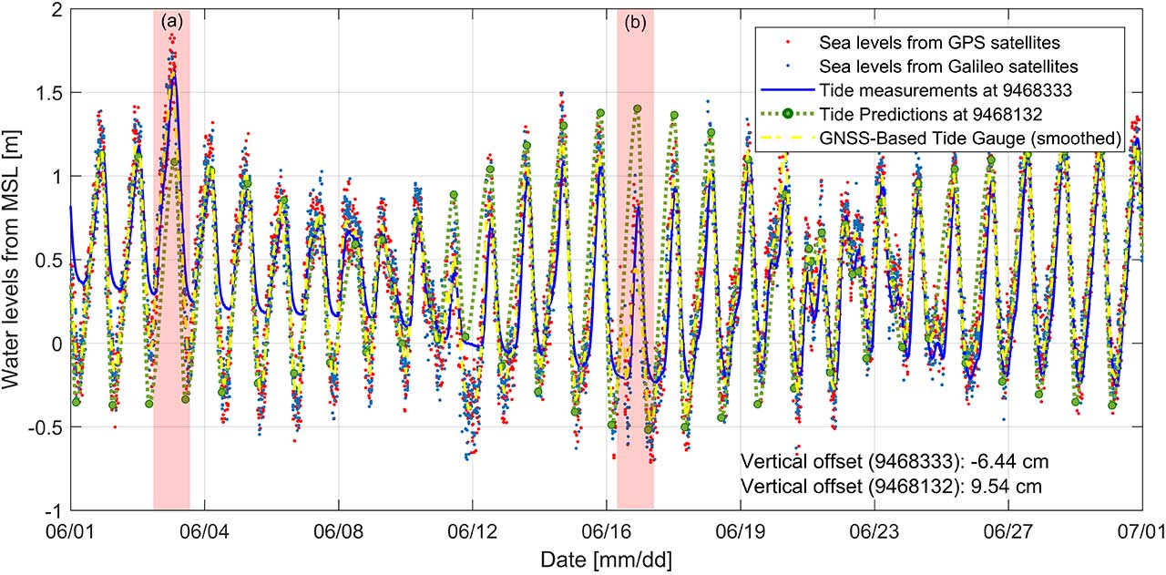
However, the vertical datum in Alaska has significant gaps in the spatially varying tidal information because of the difficulties of operating tide gauges there so that accurate information for datum conversion cannot be obtained. Therefore, the averages of the vertical differences were calculated (–6.44 centimeters for the St. Michael tide gauge and 9.54 centimeters for the Unalakleet tide gauge), which were then applied to each of the time series to make the comparisons. In fact, such a problem implies another advantage of a GNSS-R-derived tide gauge: it already returns a water-level height based on the terrestrial datum so that the datum of the land and the ocean can be consistently retained.
FIGURE 6 shows the sea level derived from the GNSS-based tide gauge measurements using GPS (red dots), Galileo (blue dots), the predicted sea level from the St. Michael tide gauge (green dots and lines) and measured sea level from the Unalakleet tide gauge (blue line).
FIGURE 6. Time series of sea level derived by GNSS-R-based tide gauge (AT01) in St. Michael, Alaska, during a month (red and blue dots for GPS and Galileo satellites, respectively; yellow dashed lines for the smoothed time series from two hours’ moving average filter) together with sea-level measurements from the Unalakleet tide gauge (blue solid line) and sea-level predictions from the St. Michael tide gauge (green dots for high- and low-tide predictions and green dashed line for interpolated predictions). (image: Authors)
The overall results show good agreement with the tide predictions at the nearby St. Michael tide-gauge station. It should be noted that the St. Michael tide gauge only provides high- and low-tide predictions so these were interpolated. However, some tidal characteristics not represented in the published predictions were also confirmed. In particular, as shown in the red-shaded segments of the time series marked (a) and (b) in Figure 6, larger and lower amplitudes than the tide predictions for the St. Michael tide gauge were identified on June 3 and 16, respectively.
These inconsistencies can be explained by the comparison with actual sea-level measurements at the Unalakleet tide gauge (solid blue line in Figure 6), which show very similar sea-level changes compared to those of the GNSS-R-based tide gauge. In addition, the overall larger amplitudes in the time series from the Unalakleet tide gauge can be explained by considering the fact that the amplitudes of the water levels vary along the coastline in Alaska and the Unalakleet tide gauge is approximately 74 kilometers from AT01.
To quantitatively investigate the agreement between the GNSS-R-based tide gauge and the standard tide gauges, we computed correlation coefficients. To ensure simultaneous data, the standard tide-gauge measurements and predictions were interpolated to the time tags of the GNSS-R-based time series. The correlation coefficients are 0.87 and 0.81 with the St. Michael and Unalakleet tide gauges, respectively.
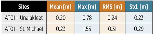
The statistical analysis of the comparison result is summarized in TABLE 1. The mean and maximum values were computed using the absolute sea-level differences. From the results, it could be established that the GNSS-R-derived sea level shows better agreement with actual sea-level measurements at the Unalakleet tide gauge even though it is approximately 74 kilometers away from AT01.
Table 1 Statistical analysis of the sea-level differences between the GNSS-R-based tide gauge (AT01) and the standard tide gauges (Unalakleet and St. Michael).
Spectral analysis was additionally conducted to validate the sea levels from the GNSS-R-based tide gauge. Because the St. Michael tide gauge does not provide actual measurements (only predictions), only the Unalakleet tide gauge was used in the spectral comparison. A fast Fourier transform (FFT) was applied to convert the time series of the sea levels to the frequency domain.
The GNSS-R-based tide gauge showed good agreement with the Unalakleet tide gauge overall. In addition, from the corresponding spectral analysis results, we were able to find meaningful harmonic constituents, M2, K1 and O1. The harmonic constituents estimated from the sea-surface measurements of the GNSS-R-based tide gauge have amplitudes most similar to the published harmonic constituents of the nearest St. Michael tide gauge, although the difference in amplitudes of the three harmonic constituents averages 12.3 centimeters.
In fact, the Unalakleet tide gauge also does not exactly match the amplitude of the estimated harmonic constituents and the published harmonic constituents. But by summarizing the corresponding results, we can conclude that the harmonic constituents estimated from the GNSS-R-based tide gauge are reliable.
As mentioned earlier, in our study, we estimated the water-level change by using GPS and Galileo satellite signals to overcome the degradation of GNSS performance due to the satellite geometry in the Arctic. The smoothed time series, calculated from a moving-average filter of two-hour intervals, is shown in Figure 6 (yellow dashed lines). The time series of sea level derived by the GNSS-R-based tide gauge during the whole month were used as ground truth for evaluating the accuracy.
This was done because the Unalakleet tide gauge is approximately 74 kilometers away from AT01 and the St. Michael tide gauge does not provide actual measurements, making it difficult to use as ground truth. As a result, the sea levels determined using the Galileo and GPS signals showed very similar accuracy with an average difference of 0.11 meters. Therefore, even if Galileo is additionally used, the estimated final water levels were at a similar level of accuracy.
However, the number of water-level observations dramatically increased (approximately doubled) when GPS and Galileo signals were both involved, even though the number of Galileo satellites is fewer than the number of GPS satellites. This is because Galileo transmits on five frequencies while GPS transmits on just three, so we can achieve more robust solutions by including Galileo.
We investigated how adding Galileo satellites changes the temporal resolution of the final sea-level measurements. At this time, several sea-level measurements pointing to the same epoch (such as sea levels from several frequency observations of the same satellite arc) were considered as one measurement for the time interval computation.
Overall, sea-level measurements using only Galileo satellites show lower temporal resolution compared to GPS satellites alone, with a mean time interval of 48.97 minutes because Galileo is not fully operational yet and fewer satellites are available. However, combining GPS and Galileo satellites to the sea-level analysis significantly increased the time resolution.
When only GPS satellites were used, the maximum time interval between two water-level measurements was greater than 3 hours, while the maximum time interval was shortened to about 1.5 hours when Galileo satellites were included in the water-level measurement.
However, even if both GPS and Galileo satellites were used, the average time interval was still 14.1 minutes, which is considerably longer than the time resolution of the standard tide gauge of 6 minutes. The lower time resolution of a GNSS-R-based tide gauge is explained by the limited ranges (azimuth and elevation angle ranges of 0° to 230° and 10° to 25°, respectively) toward the ocean at station AT01. It means the time resolution can be improved by securing a wider view of the ocean from the GNSS-R-based tide gauge.
SUMMARY AND CONCLUSION
The purpose of our study was to evaluate and verify the feasibility of using GNSS-R for sea-level monitoring in the Arctic. We used data from a GNSS station in St. Michael, Alaska, and applied an advanced algorithm that accurately determines sea levels through the comparisons of results from multiple GNSS signals along with an effective filtering procedure. Our results were validated through comparisons with measurements and predictions from nearby standard tide gauges.
From the corresponding analysis, we could confirm that the GNSS-R technique overcomes the limitations of standard tide gauges in the Arctic and successfully estimated the sea-level change in St. Michael, Alaska. The results from this study show many promising applications for a GNSS-R-based tide gauge in the Arctic, such as tsunami and flood monitoring and tidal datum determination.
In future studies, additional research should be conducted on how well the GNSS-R-based tide gauge can operate in extreme conditions such as low temperatures, wind gusts, storms, and snow. And, for further improvement of the temporal resolution of the technique, all active GNSS constellations including GPS, GLONASS, Galileo, and BeiDou should be included — that will certainly improve the temporal resolution and also potentially improve the accuracy and reliability. It would be also worth studying the spatial variations of sea-level changes by investigating the specular reflection points of GNSS multipath signals.
ACKNOWLEDGMENTS
This article is based on the paper “Monitoring Sea Level Change in the Arctic Using GNSS-Reflectometry” presented at ION ITM 2019, the 2019 International Technical Meeting of The Institute of Navigation, Reston, Virginia, Jan. 28–31, 2019.
SU-KYUNG KIM is a graduate research assistant at Oregon State University in Corvallis, Oregon. She received her M.Sc. in geoinformation engineering from Sejong University in Seoul, South Korea, in 2013. Her research interests are focused on sea-level change monitoring and crustal deformation studies using GNSS.
JIHYE PARK is an assistant professor of geomatics at Oregon State University. She holds a Ph.D. in geodetic science and surveying from The Ohio State University in Columbus, Ohio. Her research interests include GNSS positioning and navigation, GNSS reflectometry, ionospheric and tropospheric monitoring for natural hazards and artificial events, and other geospatial-related topics.
FURTHER READING
Authors’ Conference Paper
“Monitoring Sea Level Change in the Arctic Using GNSS-Reflectometry” by S.-K. Kim and J. Park in Proceedings of ION ITM 2019, the 2019 International Technical Meeting of The Institute of Navigation, Reston, Virginia, Jan. 28–31, 2019.
Pioneering Work by Manuel Martin-Neira
“The PARIS Concept: An Experimental Demonstration of Sea Surface Altimetry Using GPS Reflected Signals” by M. Martín-Neira, M. Caparrini, J. Font-Rossello, S. Lannelongue and C.S. Vallmitjana in IEEE Transactions on Geoscience and Remote Sensing, Vol. 39, No. 1, 2001, pp. 142–150, doi: 10.1109/36.898676.
“Coastal Sea Level Measurements Using a Single Geodetic GPS Receiver” by K.M. Larson, J.S. Löfgren and R. Haas in Advances in Space Research, Vol. 51, No. 8, 2013, pp. 1301–1310, doi: 10.1016/j.asr.2012.04.017.
“Monitoring Coastal Sea Level Using Reflected GNSS Signals” by J.S. Löfgren, R. Haas and J.M. Johansson in Advances in Space Research, Vol. 47, No. 2, 2011, pp. 213–220, doi: 10.1016/j.asr.2010.08.015.
“Three Months of Local Sea Level Derived from Reflected GNSS Signals” by J.S. Löfgren, R. Haas, H.-G. Scherneck and M.S. Bos in Radio Science, Vol. 46, No. 6, 2011, RS0C05, doi:10.1029/2011RS004693.
“Determination of Water Level and Tides Using Interferometric Observations of GPS Signals” by K.D. Anderson in Journal of Atmospheric and Oceanic Technology, Vol. 17, No. 8, 2000, pp. 1118-1127, doi: 10.1175/1520-0426(2000)017<1118:DOWLAT>2.0.CO;2.
Earlier Innovation Columns Dealing with GNSS Refectometry
Tides, Surges and Mean Sea-Level by D. Pugh, published originally by J. Wiley & Sons, Chichester, U.K., 1987, reprinted with corrections in 1996 and subsequently issued in e-print form by NERC Open Research Archive.
Random Sample Consensus
“Random Sample Consensus: A Paradigm for Model Fitting with Applications to Image Analysis and Automated Cartography” by M.A. Fischler and R.C. Bolles in Communications of the ACM, Vol. 24, No. 6, 1981, pp. 381–395, 10.1145/358669.358692.
In a case of fortuitous happenstance, I found myself in an operations support center for an undersea expedition with two, large, flat screens mounted on a wall peering into the deep through the remote viewer slowly gliding through a dark blue barren abyss.
The NOAA ship Okeanos Explorer. (Photo: NOAA)
Deep dive into ocean exploration
That encounter led me on a deep dive of my own into undersea expeditions and becoming this month’s article.
I have been interested the deep sea since my youth growing up in the age of Sealab and watching The Undersea World of Jacques Cousteau. Later in life, I served in the U.S. Navy and took part in one of the first successful real-world tests of a geospatially enabled, full-spectrum battlespace using tactical oceanography, which ultimately steered me into the field of Geographic Information Systems and Imagery Analysis.
That accomplishment helped in my being selected to establish one of the first operational GIS units for supporting Special Operations Forces.
After retiring from the military, I briefly worked as a nautical charts cartographer. So, from a practical perspective, for five years I worked supporting maritime, near-shore and riverine environments. However, going back another 10 years, I was formally trained in oceanography as part of my overall career in the Navy as an aerographer, which also included the disciplines of meteorology, astronomy and astrophysics.
Many years I spent observing and contemplating the ocean of air above, the waters below, and the heavens beyond. One cannot meditate upon the firmaments and assuage the wonder within. Whether for war or love, to ponder the sea and sky emotes an imprint on the heart.
Ocean, the larger part of Earth, alive and thriving, captivates our imagination. What must we, the conscious beast, have wondered when the first of us standing at land’s end looked out upon the mysterious deep of the Great Waters stretching from where he stood to the base of the celestial dome? Did he think it marked the end of the habitable world where mortals dwell and that the great expanse of waters separated us from the heavens where the sun rises and sets and where the moon and stars reside?
I shall reveal a secret; it is a mystery [of the gods] I tell you. There is a plant that grows at the bottom of the ocean, it has a prickle like a thorn, like a rose; it will wound your hands, but if you succeed in taking it, you will hold that which restores lost youth to a man.
— Utnapishtim, Epic of Gilgamesh (Sumeria 2100 BC)
Coral treasures
The Greeks, the race of ancient seafarers knew well the secrets of the sea. Aristotle, the wise philosopher of the ages, still teaches us through his pupil Theophrastus, who spoke of a deep sea plant, red and hard like a stone. He named it korallion. We call it coral.
Photo: NOAA
Aristotle also observed that sponges were better from deeper depths and invented the diving bell to collect them. Another of his students, Alexander of Macedonia, the warrior king, had a diving bell made of glass, a Colimpha, so he could walk the seafloor. Perhaps, on his conquest of Babylon, Alexander heard about the secret of Gilgamesh and sought the plant for himself. How valuable would such a plant be to a warrior king?
Corals have always fascinated man, like treasures from another world — not from this dry land called Earth ruled by air-breathing, upright beings, but from a world of water with bizarre and terrifying creatures and plants made of stone.
Photo: NOAA
Corals, as it turns out, are not a plant at all. They are the smallest of animals, called a cnidarian, and millions of them together form the broad-limbed, rock-like structures. They take many thousands of years to develop into the large, picturesque arrangements beneath the waves.
Colonies of corals form reefs. The largest of these is the Great Barrier Reef in Australia’s northeastern waters. The second largest is the Mesoamerican Barrier Reef in the Caribbean Sea. wherein lies the Great Blue Hole off the coast of Belize. The Great Blue Hole was deeply explored this summer.
Corals are the cornerstone of the ocean. By some estimates, the world’s corals are worth nearly $10 trillion, but that diminishes their real value because if they perish the ocean itself could die. Corals are the proverbial canary in the coalmine, and throughout the world they are ailing.
The ocean’s health is in decline. There have been six severe coral bleaching events in the past 30 years and they are occurring more frequently and for longer periods each time. Over 20% of the world’s corals are already gone. Saving them is a concern for us all.
The United States is leading the effort to protect the ocean’s corals and the National Oceanographic and Atmospheric Administration (NOAA) is at the forefront. The President’s Budget for 2020 funds NOAA for Ocean, Coastal and Great Lakes Research at $218.5M, which is an increase of $12.7M from FY 2018.
A team of scientists and researchers at NOAA are mapping deep sea corals in Alaska and Hawaii and along the coastlines of North America. Operations are underway aboard the Okeanos Explorer, one of NOAA’s ocean exploration vessels. It is on the second leg of Expedition 19-05 taking place from Tuesday, Aug. 27, through Sunday, Sept. 15.
The expedition begins in Canada’s largest underwater canyon, a marine protected area called The Gully 125 nautical miles (NM) off Nova Scotia, and then continuing south along the continental shelf. A deep-sea remotely operated vehicle (ROV), a modern-day Colimpha, is exploring the depths to over 10,000 feet (3,050 meters).
The ship’s location can be tracked online. Clicking on the ship icon will reveal details of the ship’s speed, heading, weather conditions and bathymetry
The Okeanos Explorer tracker allows users to follow the course of an Okeanos cruise. (Screenshot: NOAA)
NOAA’s Deep Sea Coral Research and Technology Program maintains the National Database for Deep-Sea Corals and Sponges, which is an interactive map portal with more than 650,000 records. It can be accessed here.
A Calling for the Ocean
I had the honor and privilege of interviewing Kasey Cantwell, an expedition coordinator for NOAA, after she returned from Halifax helping setup the command center for Expedition Deep Connections 2019 (EX1905).
In June and July of this year, Kasey led the Windows to the Deep Expedition (EX1903) from onboard the Okeanos Explorer, diving into a vast field of deep-sea corals known as the Blake Plateau about 100 miles off the coast of the southeastern U.S. It is one of the largest, most dense and diverse coral fields discovered at those depths.
Control room of the Okeanos. (Photo: NOAA Office of Ocean Exploration and Research)
Kasey’s seven years working at NOAA has been her dream come true. How every mission unfolds is what holds her fascination for the job. As the ROV Deep Discoverer descends, no one knows what they will find, but everyone knows they will be exploring an area never seen before.
They might find a shipwreck, or a plane crash, or a new species, or some strange geological formations. She very much enjoys listening to experts from around the world who are tuned in to the live feed from the ROV, discussing what they are seeing and — even with all that expertise — how often they are all surprised or stumped coming across something unexpected or never before seen.
Better ROVs on the Horizon
Deep-sea exploration is relatively new. Technology continuously improves. The ROV’s ability to remain in place with its high-resolution zoom camera makes exploring and observing the deep-sea environment possible like never before. New discoveries happen with almost every dive.
Limitations exist with the present class of submersibles because they are loud, bulky and bright, scaring off much of the marine life. But the next evolution of deep-sea submersibles are being developed.
The next generation will be stealthy, artificially intelligent, autonomous systems with improved battery life and a suite of sensors able to accomplish much more than we can today. Several of these submersibles will be able to operate in a network, providing us new and fascinating discoveries and observing marine life more naturally.
The best way to stay informed about NOAA’s expeditions is subscribe to NOAA’s Faceook page.
Protecting Our Oceans
America can be proud of its ocean services. NOAA is standing as the vanguard protecting our seas, balancing environmental concerns and commercial demands helping ensure our oceans remain thriving and healthy into the future.
NOAA is identifying areas to be designated as marine protected areas (MPAs) that need safeguarding. There are 15,059 MPAs in the world, and more than 10% are in U.S. waters. MPAs prevent over-fishing and minimize the effects of pollution and further damage to coral reefs and marine environments.
In closing, the biome of the sea has been under explored and undervalued, resulting in less funding, care and attention; but recent discoveries in biotechnology have scientists believing corals hold potential for medicines and life-saving drugs.
Already, more than 40,000 compounds from aquatic resources have been identified for possible medical benefits. This interest is stimulating investment into undersea exploration and development.
In the future, doctors will prescribe pharmaceuticals originating from coral farms on the ocean floor — a secret revealed over 6,000 years ago inscribed on clay tablets in the Epic of Gilgamesh, one of the earliest writings in human history.
The sea summons us to its edge providing a moonlit path by night, and by day a diadem of sparkles herald the sun.
The majestic ocean, rhythmic and soothing yet chaotic and raging, is a tempest that both calms and terrifies the soul. And we, the conscious, land-dwelling beast seeks understanding and harmony with our sister the Sea. That calling is the mission of NOAA’s Ocean Exploration Research.
Strange fluid extrusions found on the escarpment of Verrill Canyon at a depth of 7,972 feet (2,430 meters) on Aug. 30, 2019. (Screenshot: NOAA Okeanos Explorer ROV livestream)
NOTE TO THE READER: In the Epic of Gilgamesh, Utnapishtim preserved mankind from destruction, and as a reward was given eternal life. He was ferried across the “Great Waters” known as Ea, separating the land from the heavens, and sent to live in the city of Dilmun where the Sun rises. Urshanabi, the boatman, was the only one who could pass over the waters between the two worlds. Gilgamesh tricked Urshanabi into taking him in his boat to the edge of Ea to the gates of Dilmun where Utnapishtim came and told Gilgamesh the secret.