The place to be if your job is intelligence and why what is where.
By Art Kalinski
When I was in graduate school at the University of North Carolina at Charlotte, Dr. Jerry Ingalls shared a succinct description of the “new” geography. He stated that old geography was merely the study of where everything was. However, new geography, with its spatial analysis tools, had significantly expanded the field of the study to “why what is where” and knowing why we can start predicting new “wheres” based on known facts. That, of course, is where geospatial intelligence is today, and some of those tools and techniques identified the location of Iranian nuclear facilities long before they became public knowledge.
Learning about the latest tools and techniques is the primary reason for conferences, and there is agreement in the geospatial community that GEOINT is the place to be. Organized by the United States Geospatial Intelligence Foundation (USGIF), attendance at the San Antonio conference was the highest it has ever been, according to USGIF President Keith Masback. Even with a weak economy, the over-arching opinion of all attendees was that the intelligence business will continue to grow regardless of world politics. By its nature, this conference really had many more “chiefs” than “Indians,” and many exhibitors spared no expense at the conference, knowing that they were reaching key decision makers.
USGIF, a nonprofit educational organization created by the geospatial intelligence community, is the organizing force behind the conferences. There is heavy participation by the National Geospatial-Intelligence Agency (NGA) and other intelligence agencies, so the conference attracts top executives in the geospatial industry. The speaker and attendee list reads like a who’s who of the geospatial and intelligence fields.
General Clapper, the Under Secretary of Defense for Intelligence, was a keynote speaker. He stated his belief that regardless of geopolitical decisions, he sees no decrease in the need for intelligence in Afghanistan and many other locations around the world. He further addressed the need for much faster turn-around of actionable intelligence and cited the joint efforts between the SIGINT (Signals Intelligence) and GEOINT (Geospatial Intelligence) communities.
General Clapper discussed some of the work of the ISR (Intelligence, Surveillance, Reconnaissance) Task Force, which is seeking new technology and the Holy Grail of intelligence, automated target identification in complex environments. He also spoke about the benefits of commercial imagery sources and its use in an impressive NATO Fusion Center he toured.
The second keynote speaker was Representative C. A. Ruppersberger, D-MD, chairman of the House Technical/Tactical Intelligence Subcommittee. The congressman addressed his concern that the U.S. is in danger of losing its preeminence in space because regulations are hampering development. He specifically addressed a need to overhaul International Trade in Arms Regulations (ITAR) that are hurting the U.S. commercial satellite industry. He also stated the need for additional research and development funding like the ones that built the U.S. space program and a greater emphasis on technical education. A troubling statistic he cited is that China has 440,000 engineers compared to the USA’s 65,000.
Vice Admiral Murret, head of NGA, then spoke of his agency’s support not only for the military but humanitarian assistance in natural disasters such as flooding and earthquakes. He talked about the new NGA facility at Fort Belvoir and about how one third of his agency now works in St. Louis.
In the exhibit hall close to 200 exhibitors demonstrated their latest efforts. Some highlights include:
Cogent3D and Lockheed Martin demonstrated the release of GeoSketch, a plug-in for Google Sketch Up. GeoSketch permits military users to build 3D models using the easy to use Google Sketch Up software. The tool permits users to import military UAV video imagery, oblique imagery, and other photo sources to rapidly build 3D models even if geo-referencing data or camera models are missing. The models can then be exported in common formats such as Google, Multipatch, or OpenFlight.
Digital Globe announced the successful launch of its newest high-resolution satellite, WorldView 2. Imagery from the new satellite will be available in a few months, doubling Digital Globe’s image-collection capability, including multi-spectral imagery.
LEXISNEXIS news open source highlighted the tremendous wealth of data that it makes available to intelligence analysts. Appistry and NJVC had extensive information on cloud computing and their ability to deliver mission-critical data, including legacy data, to users around the world.
Pictometry and Lockheed Martin announced their alliance and creation of a new service, Intelligence on Demand (IOD). IOD promises to be a game changer. (See October’s column for details.)
Every conference I attend there is always a new technology that really catches my eye. Ball Aerospace was demonstrating such a technology, Flash LIDAR. Flash LIDAR has been a laboratory curiosity for a while but Ball Aerospace has made it a functional tool. Most current LIDAR collections use a laser to scan the ground with the return being sampled resulting in a collection of points on the ground that provide elevation data from which a DEM or contour lines are created. Although this is a rapid process it is sequential and not instantaneous. The resulting data can be very coarse or fine depending on the sampling interval.
Flash LIDAR is what the name implies; an entire area is imaged in one nano-second flash. The laser is diffused over an area and flashed once. The resultant image is a broad but dense sample taken at the same instant rather than through a scanning process. Since the image is taken from the same point at the same instant, the data can be used to create accurate 3D models. Those models can then be draped with photographic images or even video frames. The process is so fast that 3D models can be created almost in real time.
The below images are a practical demonstration of the Ball Aerospace process using Flash LIDAR combined with a live video camera. As each frame of the video image is taken, a simultaneous Flash LIDAR image is also taken from the co-located LIDAR unit. The photo shows the live video and point representations of the Flash LIDAR 3D surface and the resultant 3D image draped on the moving 3D model.
It’s hard to tell from these still 2D photos but seeing this system in operation was impressive since the Flash LIDAR and resulting 3D models were continuous and perfectly registered. The only limitation of this demonstration was that human flesh is not a good “Reflective Surface.” Note that in the photo the Ball representative was very animated. This stop-action screen-capture shows him as he jumped up. In all cases the Flash LIDAR kept up with the dynamic movements.
Point cloud.Point cloud.Point cloud.Wire-frame image.
This was an impressive conference that suffered from too much in too short a time. Two tools that were very helpful was a daily newspaper, the Show Daily, that recapped the previous day along with the current day’s schedule. It was published, printed, and placed under our doors as we slept. The other useful tool was a daily video show with key presentations and interviews for those that were unable to be in two places at the same time. It was available at several break locations and on our in-room TVs. This has been done at other conferences but not as well as the execution of USGIF.
It occurred to me that I haven’t discussed my plans for GeoSpatial Solutions (GSS) since I assumed the editorship of GSS a couple of months ago. Some of you have told me that you thought GSS had “gone away.” True, it was somewhat dormant for awhile, but we’ve got some fantastic initiatives underway for 2010 that will renew your interest in GSS.
First of all, GeoSpatial Weekly will have an opinion column (mine or a guest whom I coordinate) every issue. I’ll strive to provide something interesting to read that’s relevant every week. Sometimes there is big news to cover and sometimes there’s not, but I’ll always strive to make it interesting. We’ll also continue to produce the monthly GeoIntelligence Insider Newsletter which is focused on news and analysis of spatial technologies in the homeland security and defense segment.
As some of you may know, I am the founding editor (and continue to be) of GPS World magazine’s Survey Scene newsletter that began more than three years ago. Target marketed e-mail newsletters were a new concept for GPS World at that time, and over the past several years we’ve proven it’s the right formula for delivering valuable information to your e-mail inbox in a timely manner. Furthermore, our highly successful webinar series has drawn a tremendous amount of response from our readers.
Fortunately, GeoSpatial Solutions is a sister publication of GPS World magazine. Both are owned by Questex Media, which operates a fair number of print and digital magazines in addition to other products and services. They have a very capable IT department which can administer a number of powerful technologies like webinars and video hosting.
This gives GSS a firm leg in which to leverage from.
Currently, you may have noticed that we are piggy-backed on the GPS World website as a temporary home. Over the next couple of months, we will be redesigning the website with its own “look and feel.” We will be adding a number of sections that will make resources available to you such as archived webinars (GIS-oriented), videos, white papers and others.
A particular area where I want to pay specific attention is what I call the Survey Section. There is no doubt in my mind that land surveying professionals and GIS professionals are going to be close brethren in the geospatial world. The roles of both are evolving and the line of demarcation is not always clear, but the two need each other terribly in order to best serve the public. GIS isn’t always about parcel maps and land surveying isn’t always about coordinates. The Survey Section (or whatever better name I come up with) will be a place for this sort of knowledge exchange and collaboration in a positive way. There is not one person or company that can stop this geospatial train, so what’s left is how best the two professions can work together.
Webinars:
As I mentioned above, webinars are a powerful communication tool. Also consider that travel budgets and industry conference budgets have been chopped considerably in the “new economy,” webinars are a natural fit. Last year during the weeks before the ESRI User Conference, I dedicated a GPS World webinar to GIS. I plan to do the same this before prior to the ESRI UC in July as well as the INTERGEO conference in Europe in October. These are the two largest geospatial events.
Guest/Industry perspectives:
I tell my wife I’d hate to be married to me. Thank goodness for our family that she doesn’t always listen to me :-)
I think it’s invaluable to hear perspectives from industry folks, even if they don’t agree with me. I’ve started reaching out to those whom I think would bring an interesting perspective to GeoSpatial Solutions. Starting in 2010, I’d like to have at least one per month on varying topics from GIS database technology to trend analysis to data collection methods to new computer hardware developments that effect geospatial professionals.
Multimedia content:
The next best thing to being there is viewing a video of an event, an interview, a process, or experience of some sort.
Youtube, Google Earth and the internet in general have transformed the way we interact in our world and specifically our geospatial world. Those technologies have brought us closer. During my last webinar, I had questions from several people who lived on different continents…Asia, Australia, Europe and Africa. I was interacting with other geospatial professionals who lived in completely different cultures, spoke different languages and lived in significantly different time zones. I cannot begin to imagine kind the room he or she sat in while attending the webinar anymore than he or she could picture what my little office space looked like, but our common geospatial connection brought us together.
Multimedia content is a tremendously important technology that allows us to grow closer in the geospatial community even though our geographic coordinates are significantly different.
Industry Conference Live Coverage:
Attending major industry conferences is important to me because that’s where a lot of industry buzz is taking place and where I get a chance to meet up with a lot of people with whom I don’t see on a regular basis. I also tend to present at these conferences too. The next one is the ACSM/GITA conference next Spring in which I’m leading a half-day GPS workshop along with Pamela Fromhertz of the National Geodetic Survey.
Live coverage of conferences is a great way of bringing you closer to the conference buzz from your desktop at work or home especially when combined with blogging (such as what we’ve done at GPS World) and video coverage.
KSA (keyword search) Service:
Soon, we will give you the ability to sign up for KSA free of charge. Essentially, you select from a list of keywords (such as web-mapping, WAAS, GeoPDF). Once signed up, we will automatically send you an e-mail every time new content (news stories, columns, webinars, etc.) is published that include your keywords.
Blog/Twitter/Discussion Forum:
There is a notion of utilizing too much technology. I want to be careful of that. Blog’s make sense if they are relevant and insightful. Twitter is the fast-food of the blog world.
Discussion forums can be very useful, but they are only powerful if there is participation from a lot of users. That can only happen if there is a foundation of relevant and useful content.
I can’t tell you if we will use these technologies, but I can tell you that if we do, we will do it right. I respect your time and attention enough to not want to waste it.
ABB has selected Intergraph for the development of an oil and gas pipeline network and relevant facilities in North Africa. The pipeline network will be built in the El Merk field, a remote, harsh desert location in Algeria.
According to Intergraph, geospatial-based pipeline infrastructure management solutions will enable ABB to more effectively design, construct and maintain pipelines and assets and demonstrate a comprehensive pipeline integrity program while reducing the cost of maintaining records. By storing records in a central geographic information system (GIS), the solution makes information readily available for a variety of applications, improving record keeping productivity while assuring compliance with regulatory requirements.
“An accurate, up-to-date view of all critical assets at any given time is a crucial component of any pipeline implementation project,” said Sergio Casati, ABB Project Manager. “Especially in such challenging terrain conditions, we need to keep our pulse on the status of all assets in near real-time. The strength of Intergraph technology and its more than 40 years of experience in the utilities sector, as well as market leadership in enterprise engineering software, were key factors in our decision to partner with the company on this project. Intergraph’s open, flexible technology platform was also desirable for an initiative like the El Merk project, which involves a consortium of multiple vendors.”
The announcement said that geospatial technology from Intergraph will play a significant role in the design and installation of the pipeline, field gathering stations, gas distribution manifolds, flow and trunk lines and water and gas re-injection facilities in El Merk. The technology will support the Pipeline Open Data Standard (PODS) model, the most widely implemented pipeline data model in the industry, and all data will be stored in an Oracle Spatial database. The implementation will also include a portal component for the seamless distribution of data to all parties, including field and remote users.
“The collaboration of Intergraph with ABB Italy on this project marks a significant milestone in Intergraph’s involvement in the oil and gas pipeline industry,” said Maximilian Weber, Utilities & Communications manager for Intergraph in EMEA. “Intergraph has worked with leading pipeline providers around the world including Spectra Energy and Northwest Energy in the U.S., E.ON Ruhrgas in Germany and Chongqing Gas in China. Additionally, our Process, Power & Marine division is the world’s leading provider of enterprise engineering software for the design, construction and operation of plants, pipelines, ships and offshore facilities. We are pleased that ABB has recognized our strength in this industry and has chosen us to ensure the accurate, efficient management of assets, as well as play a key role in protecting this infrastructure.”
Years ago, I heard a funny joke/maxim. I repeat it often and so do several others I know of so maybe you’ve heard it.
“What’s the difference between a used car salesman and a GPS salesman?”
Answer: The used car salesman knows when he’s lying to you.
I didn’t attend the Minnesota GIS/LIS Annual Conference last week, but I received a report from someone who attended a session in which the presenter seemed to fit the maxim quite well. One of the presenter’s messages was that people should stop using WAAS immediately as a GPS correction source due to the inability of data collection software to handle the ITRF00 > NAD83/CORS96 datum shift. Following is a statement from one of his slides…
“WAAS Real-time accuracy degraded because of datum shift”
He claimed that users are “in a panic over it.” In all fairness, the presenter could have very well understood that the datum shift can be handled by a number of data collection software packages…just not the one he represents. After all, he works for a local distributor of GPS equipment. Or, even a scarier scenario would be that he really believed what he spoke.
I’m not interested in naming names or company names of the offending party, but rather painting the true picture. Of course, the attendee I mentioned above knew better than to believe what the presenter was pitching. His group has been using WAAS as a primary correction source for a number of years and reconciling the datum shift between ITRF00 and NAD83/CORS96. It’s not that hard folks.
Let’s review.
ITRF00 is essentially the same as WGS-84(G1150) for sub-meter mapping purposes. WAAS (as well as EGNOS and MSAS) are referenced to ITRF00. You need to be aware that the definition of ITRF/WGS-84 has changed over time. Here is a link to a NIMA WGS-84 document that describes earlier versions of WGS-84 and here’s a link to the current version of WGS84 (G1150) that was adopted in 2002.
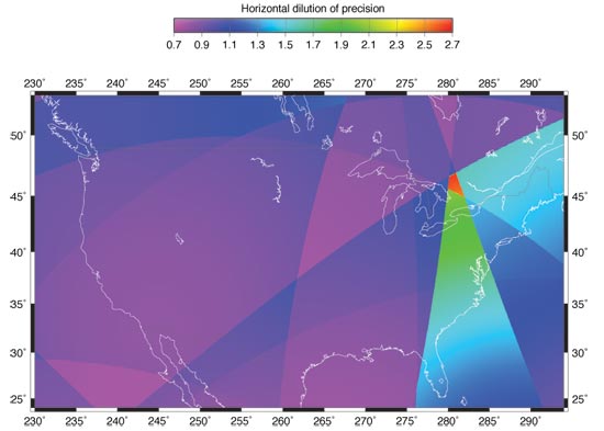
In North America (my apologies to readers from other countries), the generally accepted mapping datum is NAD83. NAD83 has also changed substantially over time. Whereas the original WGS-84 was consistent with the original NAD83 (NAD83/86), today there is a substantial difference between the current WGS-84(G1150) and NAD83/CORS96 and also NAD83/NSRS2007. Here is a graphic from Joel Cusick of the U.S. National Park Service that gives you an idea of the difference over North America:
Sadly and surprisingly, some data collection software today and even some PC-based “GIS” software still treat WGS-84 and NAD83 as the same. This instantly introduces a few feet of error. The irony is that people spend thousands of dollars purchasing high-performance GPS/GIS receivers capable of sub-meter accuracy only to introduce several feet of error by using software that improperly handles the datum transformation.
What’s the solution if your software doesn’t handle the datum transformation properly?
As mentioned above, WAAS is based on the ITRF00 datum and not NAD83/CORS96. As most base maps in North America aren’t referenced to ITRF, most likely you’ll need to transform your WAAS-corrected coordinates to NAD83/CORS96. This can be done one of two ways:
As mentioned above, use GPS/GIS data collection software that handles the transformation correctly. This makes the transformation transparent, painless to the user and accurate in real-time.
Apply a datum shift after you’ve collected your data. You can compute the shift by accessing an NGS datasheet near your project area (within 25 miles is close enough). Make sure it was occupied using GPS. Better yet, use coordinates from a CORS. The datasheet will report coordinates in both ITRF00 and NAD83/CORS96. Here is an example of coordinates from the CORS at Wisconsin Point, WI (near Duluth where the MN GIS/LIS Annual Conference was held):
ITRF00 Position (Epoch 1997.0) – N 46 42 18.20201, W 092 00 54.760208
NAD83/CORS96 Position (Epoch 2002.0) – N 46 42 18.17201, W 092 00 54.73394
Simply enter the two coordinates into your favorite mapping software and you’ll be able to compute the distance and direction of the difference.
Once you know this, you can apply the same offset to all of the data for your project. Quick and dirty? Yes. We’re not splitting hairs. WAAS isn’t delivering cm-level accuracy so this sort of transformation is more than adequate…and very efficient.
The fact of the matter is that many, many organizations have adopted WAAS as a primary source of GPS corrections and are dealing with this datum transformation issue on a daily basis.
Last week, I failed to mention that SBAS (WAAS, EGNOS, MSAS) is a valuable contributor to RTK users. Although not designed specifically to aid RTK ground users, some GPS receiver designers have exploited the value of SBAS satellites to enhance RTK operations. In North America, there are two SBAS satellites. In Europe, there are two and there are two in the Japan region. Following is a graphic depicting the regional coverage of the SBAS satellites and their approximate location.
In many regions of the world, users have at least one SBAS satellite available in view. The beauty of SBAS satellites for RTK is that, unlike GPS satellites, SBAS satellites are geostationary. The are available 24/7 as long as their signal path isn’t blocked by trees, terrain or buildings.
Since using SBAS satellites for RTK is a relatively new innovation within the past couple of years, not all manufacturers have jumped on the bandwagon yet. The slow adoption of GLONASS was similar. This causes a problem when users want to mix and match RTK receivers from different manufacturers. For example, a user purchases an SBAS-capable L1/L2 RTK rover to be used with their existing L1/L2 RTK reference station. If their existing L1/L2 RTK reference station doesn’t support SBAS for RTK, then the feature on their new RTK rover is worthless.
Even more important is the lack of support from RTN software designers. “No one’s asking for it” is the answer I get from RTN operators when asked if they are interested in supporting SBAS correctors in their RTN. I believe that users aren’t asking for it because users don’t have a clue how it would help them, and frankly, 99% don’t know the technology even exists. Now, if you would ask users if they’d be interested in one or two extra observables for RTK that would be
available 24/7 in a geostationary orbit every day, I bet you’d hear some really positive answers.
RTK users need to be able to utilize every observable that could help them. As Rob Lorimer and I reported last year in our market research report, machine control (based on RTK) will be the fastest growing GNSS segment over the period 2008-2012.
The usage of three dimensional data in the geospatial industry is in its infancy. It makes sense to me. Sometimes, it’s hard enough for folks to obtain and maintain accurate two dimensional data, not to mention elevation! However, as geospatial technology continues to evolve, the availability of 3D geospatial data will evolve. I’m pretty sure that in ten years we will look back and be amazed at how little we used 3D geospatial data.
But for now, what the heck are Mean Sea Level, ellipsoidal height, orthometric height, geoid height?
Sources of accurate elevation data are difficult to find. Typically, you’re going to find elevation data from aerial photogrammetry projects, LiDAR missions or from GPS data collection projects. Since availability of this sort of data on the world-wide web isn’t as prevalent as 2D geospatial data, 3D geospatial data utilization isn’t main stream yet.
There’s also the issue of the definition of elevation. Yes, just like there are differential horizontal datums, there are a variety of elevation datums. On legacy paper maps, elevations are typically displayed with respect to Mean Sea Level (MSL). MSL is an the elevation reference for local areas, but the Earth is not like a bathtub where gravity has an equal impact on the water in the bathtub that forms a smooth surface. MSL around the world varies tremendously. 2 meters MSL in New York is orders of magnitude different than 2 meters MSL in Hong Kong.
MSL is a complicated subject in itself. Check out this web page on the National Geodetic Survey’s web site that provides definitions related to MSL. The Earth is not a perfect sphere and gravity influences vary by region. For centuries until recently, elevations were stated with respect to sea level because that was the most reliable and widely known reference.
In fact, following are a couple of graphics from the NGS as well as one from Dr. Roman’s presentation that draws a clear picture of how GPS heights are related to MSL.
H = Orthometric height (Mean Sea Level), h = Ellipsoidal height, N = Geoid height
Note that the height determined by GPS is the ellipsoidal height, not Mean Sea level. The difference between the two can be tens of meters.
Most GPS receivers have a rough model of the Geoid height built into it. However, it’s very rough and can be a few meters in error. To resolve this, significant efforts have been made in the two decades to create high resolution geoid models. Creating a high resolution geoid model (for a country) is a relatively large effort that requires very skilled people and specific equipment.
Following is a similar graphic illustrating North American Datum of 1983 and GEOID03, which was the most recent geoid model of the United States (GEOID09 was just released).
Finally, following is a graphic from Dr. Fraczek that depicts the relationship between the ellipsoid, MSL and the Earth’s surface. You can see here that at some points, the ellipsoid is actually above the geoid and at some points, it’s below the geoid.
The purpose of this column is to point out that when you receive 3D geospatial data, you should inquire what about the elevation data is referenced to. Are they ellipsoidal elevations? Are they MSL elevations? If MSL, what was the resolution of the geoid model used?
Flushing out horizontal datum inconsistencies in your GIS is, for the most part, pretty straight-forward. The 2D view is the norm and once you bring data into your GIS, you can compare the imported features to the existing features and identify fairly quickly if there’s a problem with the 2D data. The problem is that most GIS folks aren’t used to working in a 3D world. I speculate that most people figure that if the 2D data is reasonable, then the elevation (if it exists in the database at all) must be accurate. It would be interesting to hear from folks who are making a concerted effort in quality checking the heights used in their GIS.
Even though GIS horizontal data is still far from perfect with respect to accuracy, at least I can see the road to success. The quality of horizontal data in the past ten years has improved significantly thanks to widespread availability of data collected via remote sensing and GPS data. I think that trend will continue as the widespread availability of accurate horizontal data continues to improve. The roadmap for 3D data isn’t so clear. Not only is there a lack of accurate 3D data, but also the models (eg. geoid model) for generating accurate 3D data continue to evolve.
Applications for 3D data are expanding and are going to continue to expand. People, both inside the geospatial industry as well as the general public, still have a hard time visualizing 3D data. For example, a land development plan for a site can be communicated much more effectively if there’s a 3D visualization (either still image or animated video) that accompanies the engineering drawings. Following is a visualization of a particular golf course hole where the architect was trying to convey the design change to the golf course owner. The image on the top is the existing golf course. The image on the bottom is the proposed design. The data used to create the terrain model in these images was high quality 3D geospatial data.
Four Galileo in-orbit validation (IOV) satellites scheduled to launch next year have already missed their first pad date.The European version of Russia’s Soyuz rocket is now scheduled to carry the four IOV satellites into orbit in two launches in November 2010 and early 2011, as announced by European Space Agency (ESA) Director-General Jean-Jacques Dordain on October 9.
Both launches had been set for earlier in 2010, but ESA has encountered difficulties with the satellites, built by a consortium led by Astrium Satellites and Thales Alenia Space. Introduction of Russia’s Soyuz rocket at Europe’s Guiana Space Center in French Guiana, on the north coast of South America, has also been repeatedly delayed.
The European Union and ESA plan to select a builder for the remaining 28 satellites late this year. Final bids from 11 companies bidding for on six Galileo work packages are expected by November 11.
Experimental Satellite Moved. In July and August, Surrey Satellite Technology Ltd (SSTL) repositioned GIOVE-A, the first Galileo test satellite, to an orbit 113 kilometers above the orbit that the operational Galileo navigation satellites will occupy.
Since its December 2005 launch, GIOVE-A has achieved all of its mission objectives and remains in excellent condition well beyond its design life of two years, SSTL stated.
The test satellite secured the Galileo frequency filings with the International Telecommunication Union (ITU), collected data to characterise the medium-Earth Orbit (MEO) environment, and flight-proved technologies such as highly accurate atomic clocks.
GIOVE-A remains fully operational, and has sufficient propellant remaining for further maneuvers. A further repositioning exercise may be performed to raise the orbit higher still before GIOVE-A is finally decommissioned.
SSTL and its new owner, OHB of Germany, jointly form one of the two consortia now bidding for the development and construction of 28 satellites for the operational Galileo service.
EGNOS. The European Commission (EC) declared on October 1 the official start of operations by the European Geostationary Navigation Overlay Servic (EGNOS), with its Open Service available free of charge to businesses and consumers. EGNOS is Europe’s first contribution to satellite navigation and a precursor of Galileo, the global satellite navigation system in development.
EGNOS is a satellite-based augmentation system that improves the accuracy of satellite navigation signals over Europe. The system is composed of transponders aboard three geostationary satellites hovering high above the Eastern Atlantic and the European continent, linked to a ground network of about 40 positioning stations and four control centers, all interconnected. The EGNOS ground stations receive signals sent out by GPS satellites. Information on the accuracy and reliability of these signals is relayed to users via the geostationary satellite transponders. This allows them to determine their position to within two meters in real-time, according to EC spokespersons.
The EGNOS coverage area includes most European states and has the built-in capability to be extended to other regions, such as North Africa and European Union neighboring countries.
The commission seeks to support new applications in sectors such as agriculture (high-precision spraying of fertilizers) and transport (for example, automatic road-tolling or pay-per-use insurance schemes). EGNOS can also support much more precise personal navigation services, both for general and specific uses, such as systems to guide blind people and to improve signal reception in urban areas.
EGNOS will be certified for use in aviation and other safety-critical areas in compliance with the Single European Sky regulation. Through EGNOS a safety-of-life service is expected to be in place by mid 2010. This service will provide a valuable warning message informing the user within six seconds in case of a malfunction of the system. A commercial service is under test and will also be made available in 2010.
EGNOS operations are managed by the European Satellite Services Provider, ESSP SaS, a company based in Toulouse, France, founded by seven air navigation services providers. A contract between the EC and ESSP SaS covers management of the EGNOS operations and maintenance until the end of 2013.
The EGNOS Open Service is accessible, without service guarantee or resulting liability, to any user equipped with a GPS/SBAS compatible receiver within the EGNOS coverage area. Most receivers sold today in Europe meet that requirement. No authorization or receiver-specific certification is required.
GLONASS Signal Generates Slip
A planned late-September launch of a three new GLONASS-M satellites from the Baikonur space center was postponed due to a problem with signals emanating from a previously launched GLONASS-M satellites, now on orbit. Initially, a new launch date of October 29 was set by Roscosmos, the Russian space agency, but no word had yet come at press time regarding investigation of a problem with the signal generator aboard the orbiting satellite, detected in late August. The spacecraft was taken out of service on August 31.
GPS Wiggles: SVN49, CNAV
The GPS Wing held an extraordinary session at ION GNSS in Savannah, Georgia, September 23, frankly explaining the SVN 49 satellite’s problem and probable solutions.
SVN49, the IIR-M) + L5 civil-signal satellite, will be set healthy in the coming months and it will be useable, the GPS Wing said. Its L1 an L2 signals contain a pseudorange error that remains within specifications for compliant GPS user equipment.
On the ground, a receiver sees from this satellite both a direct signal and a weaker reflected signal, which looks like a multipath component. According to models, if the direct and reflected L1 signals are in phase at zenith, a standard code-correlating receiver will measure a C/A-code pseudorange that is 1.62 meters too long. The error becomes smaller as the elevation angle drops, reaching zero at an elevation angle of about 42 degrees, and then rising slightly as the elevation angle drops to zero.
During audience input following the Savannah panel presentations, Javad Ashjaee of JAVAD GNSS proposed simply turning the satellite on as is and using it as an opportunity, given the “defined multipath” that it effectively transmits, to study multipath and other phenomena. JAVAD GNSS Triumph receivers have demonstrated the ability to remove almost all anomalies and satellite multipath from the SVN49 signal.
An as-yet-unconfirmed report has it that U.S. Air Force representatives and others, in an informal meeting after the session, came to a provisional agreement as to the best course. However, this has not yet worked its way through channels nor been announced.
New Message. The first test of the CNAV navigation message format to be used in the future on Block IIR-M and IIF satellites was announced at the September CGSIC meeting in Savannah, and will begin soon. A Type 0 message will be broadcast on the L2C signal by SVN49. By the end of the year, this message is to be switched on, on all IIR-M satellites. However, this initial message type will not contain useful information for end users.
Message Type 0 consists of a 12-second, 300-bit long message including the preamble, satellite pseudorandom noise (PRN) number, message type ID (=0), GPS time of week, a sequence of alternating 1s and 0s, and a cyclic redundancy check (CRC) parity block. The GPS time of week will change every 12 seconds, as will the CRC bits.
Penny Axelrad Honored
Penina Axelrad, professor of aerospace engineering sciences at the University of Colorado, received the Institute of Navigation’s 2009 Kepler Award for her “contributions in the field of satellite navigation and dedication to the education of future generations of navigation engineers.”
Axelrad has done advanced research in topics including receiver autonomous GPS integrity monitoring (RAIM), GPS bistatic radar, satellite formation flying using GPS, GPS-based orbit and satellite attitude determination, and multipath characterization, modeling, and mitigation.
She received a Ph.D. in aeronautics and astronautics from Stanford University and S.B. and S.M. degrees from the Massachusetts Institute of Technology. She has taught for 17 years at the University of Colorado.
The September “Innovation” column in this magazine, “It’s Not All Bad: Understanding and Using GNSS Multipath,” by Andria Bilich and Kristine Larson, mentions the use of multipath in studying soil moisture, ocean altimetry and winds, and snow sensing. An experiment the authors conducted, designed to study soil moisture, yielded a surprise bonus: a new methodology for measuring snow depth via GPS multipath. It has important implications for weather and flood forecasting, and could also bring new insight to bear on GPS antenna design.
In the “Innovation” column, the authors wrote, “Motivated by our studies showing that multipath effects could clearly be seen in geodetic-quality data collected with multipath-suppressing antennas, we proposed that these same GPS data could be used to extract a multipath parameter that would correlate with changes in the reflectance of the ground surface. . . .
“We carried out an experiment designed to more rigorously demonstrate the link between GPS signal-to-noise ratio (SNR) and soil moisture. Specifically, we were interested in using GPS reflection parameters to determine the soil’s volumetric water content — the fraction of the total volume of soil occupied by water, an important input to climate and meteorological models. Traditional soil moisture sensors (water content reflectometers) were buried in the ground at multiple depths (2.5 and 7.5 centimeters) at a site just south of the University of Colorado.”
Here Comes the Storm. During the experiment, two late-season snowstorms swept over Boulder. Larson and colleagues discovered that changes in multipath clearly correlated with changes in the snow’s depth, as measured by hand and with ultrasonic sensors at the test site. While it has been long recognized that snow can affect a GPS signal, this demonstrates for the first time that a standard GPS receiver, antenna, and installation — deliberately designed to suppress multipath — can be used to measure snow depth.
On September 11, Geophysical Research Letters, published by the American Geophysical Union, featured an article titled “Can We Measure Snow Depth with GPS Receivers?” by Larson and Felipe Nievinski of the Department of Aerospace Engineering Sciences, University of Colorado; Ethan Gutmann and John Brown of the National Center for Atmospheric Research; Valery Zavorotny of the National Oceanic and Atmospheric Administration; and Mark W. Williams, from UC’s Department of Geography, all based in Boulder.
The authors adapted an algorithm used for modeling GPS multipath from bare soil to predict GPS SNR for snow, introducing a uniform planar layer of the snow on the top of soil. The algorithm treats both direct and surface-reflected waves at two opposite circular polarizations as plane waves that sum up coherently at the antenna. They write:
“The amplitude and the phase of the reflected wave is driven by a polarization-dependent, complex-value reflection coefficient at the upper interface of such a combined medium with a known vertical profile of the dielectric permittivity e. The reflection coefficient is calculated numerically using an iterative algorithm in which the medium is split into sub-layers with a constant e. For the soil part, we use a known soil profile model that depends on the soil type and moisture. For frozen soil, soil moisture (liquid water) is low, as for very dry soil. For the snow part, we take a constant profile with e, considering relatively dry and wet snow layer thicknesses.
“After calculating the complex amplitude of the reflected wave at each polarization, we multiply it by a corresponding complex antenna gain. The same procedure is applied to the complex amplitude of the direct wave. After that, the modulation pattern of the received power, or the SNR, as a function of the GPS satellite elevation angle is obtained by summing up coherently all the signals coming from the antenna output and taking the absolute value square of the sum.”
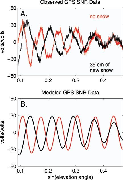
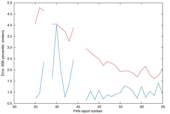
Figure 1(a) shows GPS SNR measurements for one satellite on the day immediately before and the day immediately after an overnight snowfall of 35 centimeters (roughly 10 inches). Figure 1(b) shows the corresponding model predictions for multipath. The two figure portions amply demonstrate that the multipath has a significantly lower frequency if snow is present as compared with bare soil. The authors further noted that the model amplitudes do not show as pronounced a dependence on satellite elevation angle as the observations, and state the necessity of further work on antenna gains in order to use model amplitude predictions.
Figure 1. (a) GPS SNR measurements for PRN 7 observed at Marshall GPS site on days 107 (red) and 108 (black) after direct signal component has been removed. Approximately 35 centimeters of snow had fallen by day 108. (b) Model predictions for GPS multipath from day 107 with no snow on the ground (red), and day 108 after 35 centimeters of new snow fall had accumulated (black) using an assumed density of 240 kg m-3 (figures reproduced by permission of American Geophysical Union).
How Deep the Snow. The authors propose that the hundreds of geodetic GPS receivers operating in snowy regions of the United States, originally installed for plate deformation studies, surveying, and weather monitoring, could also provide a cost-effective means to estimate snow depth.
Currently, a few conventional monitor points measure snow depth, but only at that point, and the data does not extrapolate well. Snow forms an important component of the climate system and a critical storage component in the hydrologic cycle. Accurate data of the amount of water stored in the snowpack is critical for water supply management and flood control systems. As more snow falls at higher elevations, varying greatly even within one valley or watershed, current remote-sensing snow monitors do not supply adequate data. Further, snow may be redistributed by wind, avalanches, and non-uniform melting, so that continuous data would be very helpful.
Using GPS multipath to map snow depth could improve watershed analyses and flood prediction — and, carried steps further, produce data to help better understand multipath, bringing innovation to future antenna designs.
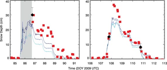
FIGURE 2. Snow depth derived from GPS (red squares), the three ultrasonic snow depth sensors (blue lines), and field measurements (black diamonds). Bars on field observations are one standard deviation. GPS snow-depth estimates during the first storm (doy 85.5–86.5) are not shown (gray region) because the SNR data indicate that snow was on top of the antenna.
Kristine Larson was featured as one of the “50 GNSS Leaders to Watch” in the May 2009 issue of GPS World.
Manufacturer
For the experiment a Trimble NetRS receiver was used with a TRM29659.00 choke-ring antenna with SCIT radome, pointed at zenith.
Photos from the GPS World Leadership Dinner 2009, September 24
ION GNSS 2009 Conference, Savannah, Georgia
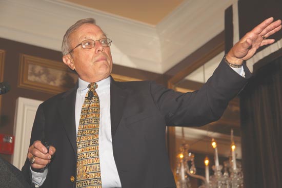
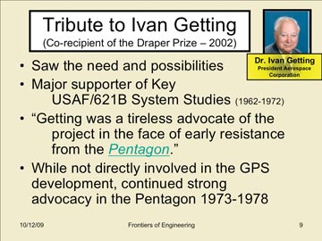
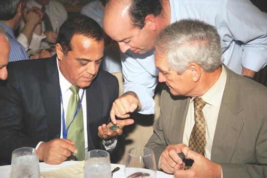
Bradford W. Parkinson, the first GPS Program Office director, chief architect, and advocate for GPS, relates “The True Story of the Origins of the Global Positioning System” and pays tribute to many of the people he worked with during that time.A slide from Parkinson’s presentation, which drew from previously classified reports as early as 1964–66. A text version of his history lesson will appear in an upcoming GPS World magazine.Keynote speaker Brad Parkinson with the evening’s hostess, publisher Kristina Panter.It’s hard to tell which shines brighter, the crystal chandeliers in Savannah’s Olde Pink House ballroom, or the many GNSS luminaries in attendance. Also sponsoring the Leadership Dinner were ITT and Spirent (Silver), and Trimble (Bronze).Greg Turetzky of SiRF Technology shows off his newest chip to Javad Ashjaee and Tom Hunter of JAVAD GNSS.
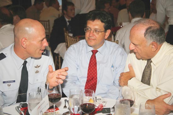
Col. David Goldstein, GPS Wing, converses with Art Gower of Lockheed Martin and Len Jacobson, Global Systems and Marketing (both members of GPS World’s Advisory Board).Lockheed Martin Space Systems was a Gold Sponsor of the dinner. From left are Todd Bender, Mike Shaw, Nancy Fitzgerald, Dan Hennessey, Bob Wright, Tom Hollenbach, and Daniel Reigh.
(from left) Sherman Lo, Stanford; Dennis Akos, U. Colorado/CSR; Mikel Miller, U.S. Air Force, ION president.(from left) Tomoya Shibata, Copla Corp.; Hiroshi Nishiguchi, Japan GPS Council; John Wilde, DW International.(from left) Carl Andren, ION; Donna Reay, Galileo Supervisory Authority; Hermann Ebner, European Commission, Galileo Unit.(from left) Attila Komjathy, JPL; Thomas Pany, iFen GmbH; Chaminda Basnyake, GM; Tom Nagle, GPS Wing.
It appears that the GPS satellite constellation has a glass ceiling, so to speak.
GPS was designed as a 24-satellite constellation, with four satellites in six orbital planes arranged to provide maximum observability around the globe. According to the government’s Space-Based Positioning, Navigation, and Timing website, “The U.S. government is committed to provide a minimum of 24 operational GPS satellites on orbit, 95 percent of the time. The U.S. Air Force launches additional satellites that function as active spares to accommodate periodic satellite maintenance downtime and assure the availability of at least 24 operating satellites. As of August 28, 2009, there were 35 satellites in the GPS constellation, with 30 set ‘healthy’ to users.”
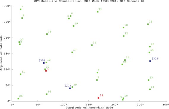
Figure 1 shows the locations of the 35 satellites. Green squares indicate satellites marked healthy in the broadcast almanac. The numbers displayed are the satellites’ pseudorandom noise (PRN) codes. Red squares, with PRN codes, indicate satellites transmitting L-band signals but currently set unhealthy. Note that SVN24/PRN24, although active, is not included in almanacs. Blue squares indicate reserve satellites with space vehicle numbers (SVNs) in parentheses. Notice the bunching together of certain pairs of satellites. The constellation of 30 healthy satellites is not configured to maximize geometrical performance. Rather it is to help guarantee a minimal level of performance considering that many of the spare satellites are one component away from failure. Basically, the 30-satellite constellation is actually being flown as a 24-satellite constellation.
Figure 1. Locations of the 35 current GPS satellites: green squares denote satellites marked healthy in the broadcast almanac, satellites marked by red squares transmit L-band signals but are curerently set unhealthy, and blue squares indicate reserve satellites. Bunched pairs show satellites being flown in tandem.
But with 35 satellites in working condition, why are only 30 set healthy? Modern GPS receivers can handle all 32 PRN codes, and many studies have shown the more satellites the better as far as position accuracy and reliability are concerned. In fact, a recent Air Force Space Command article stated, “One additional GPS satellite can make a difference between getting a degraded GPS signal and getting an accurate GPS-based location, whether it is for warfighters in Baghdad or firefighters in Boston.” The current control system should, in principle, be able to handle 32 healthy satellites.
Ground Control System. But, according to the GPS Wing, the de facto limit is 31 satellites. We don’t know if this is a problem related to 2nd Space Operations Squadron (2SOPS) functions or if there is some military system or equipment platform that cannot tolerate 32 healthy satellites.
Further, if the de facto limit is 31 satellites, why have we had only a maximum of 30 satellites set healthy since early this year? After all, 2SOPS rightly crowed about having 31 satellites set healthy for the first time on February 27, 2008, when SVN23 was reintroduced into the healthy constellation as PRN32.
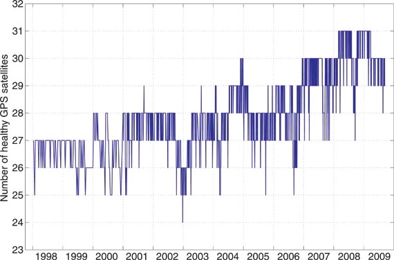
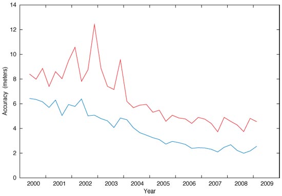
Figure 2, courtesy of Ted Driver at Analytical Graphics, Inc., shows the number of satellites set healthy from 1998 onward, according to the Notice Advisories to Navstar Users (NANUs) issued by 2SOPS and the almanacs broadcast by the GPS satellites. Often, a satellite is actually set unhealthy for only a portion of the day, but this plot tallies only the number of satellites healthy for a full day. As we can see, off and on through most of 2008 and into 2009, we had 31 satellites set healthy on orbit. With 31 satellites, users benefited from better availability and accuracy and were slightly better able to handle the occasional three-satellite outages due to SVN35/PRN5 and SVN25/PRN25 being set unhealthy for extended overlapping periods.
Figure 2. The number satellites set healthy since 1998 (courtesy of Analytical Graphics, Inc.)
But since March 26, 2009, when SVN35/PRN5 was decommissioned from active service, we have not seen a return to 31 healthy satellites.
Why is that?
Ground Testing. I asked this question to Col. Dave Madden, the GPS Wing commander, during a panel discussion on GNSS program updates at The Institute of Navigation’s GNSS 2009 meeting in Savannah, Georgia, in September. Apparently, the reason why 31 satellites cannot currently be set healthy simultaneously has do with ground testing of Block IIF satellites. One PRN code is needed for the test satellite on the ground. Presumably this means that testing involves tracking the constellation in space and a IIF test satellite simultaneously.
So, although everyone acknowledges that more GPS satellites are better, we have hit a 30-satellite ceiling. As IIF satellites are launched and further improvements are made to control system operations, and any incompatible old military systems are replaced or updated, perhaps we can break through this glass ceiling and have 31 or even 32 healthy GPS satellites available to users.
Wednesday evening, September 23, Savannah, Georgia, 5:30 to 7:00 p.m., Session P2b — a date that will live in GPS history. The 400 to 600 of us who were there to witness it will never forget it. The SVN-49 Review Panel.
Unprecedented puts it mildly.
The ION program read: “SVN49 (GPS IIR-M 20) was launched in March of 2009 to support GPS constellation sustainment as well as to bring into use the new third civil signal, the L5. During the early orbit check out of this satellite, out-of-family measurements were observed impacting the legacy GPS L1 and L2 signals. The panel will review the background, current status, issues, and options moving forward with SVN49.”
Col. David Goldstein, chief engineer, GPS Wing, gave a frank and open history and description of the situation. The panelists explained the options under consideration for partial fixes — a complete fix and eradication of the pseudorange error is not possible — and added a few remarks, but were mostly there to answer questions and provide perspective in response to opinions from the floor.
It reminded me — now this is a leap — of a climb I led in days of yore up Mt. Kilimanjaro. Or escorted, really; the Swahili-speaking Tanzanian porters did all the leading. About two days in and a third of the way up, we realized that because of a schedule change we had made earlier for longer safari in the Selous, we didn’t have quite enough time to climb the mountain in the accepted manner and still make it back down for the once-weekly flight out. So over muesli and mangos the next morning in the A-frame hut, I just threw it open to everyone and said, “It’s your trip. What do you want to do?”
Folks said later that in decades of group travel, they’d never seen the like.
Basically, that’s what Col. Goldstein, Col. Madden, and the GPS Wing did. Just threw it open. “It’s your signal. What do you want to do?”
The most likely solution may involve a partial adjustment to the signal, and then setting it useable with the caveat that it will not perform to the same degree of accuracy as other satellites, nor uniformly for all receivers.
Javad Ashjaee of JAVAD GNSS had an interesting suggestion, which basically amounted to what my teenagers sometimes tell me: “Deal.” That is, just turn it on, and away we go. Use the anomaly to study multipath phenomena. Of course, he is in the enviable postion of having, or producing, receivers that can separate out the so-called defined multipath element.
However it pans out, I commend the GPS Wing for taking such an open, public, and when you come right down to it, honest approach. I heard a bit of grumbling behind the scenes that some protocols were not adhered to in going so public. But you know what? That’s how things get done, as opposed to bogging down under cover.
And that Kili thing. We did make it up the mountain. Some of us. Sick as all getout from the altitude. Glad to come down. But we made it. Same’s gonna happen with this SVN.
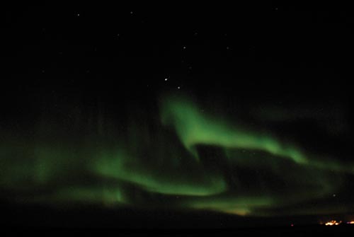
AURORA BOREALIS seen from Churchill, Manitoba, Canada. Ionospheric scintillation research can benefit from this new method. (Photo: Aiden Morrison)Photo: Canadian Armed Forces
By Aiden Morrison, University of Calgary
Two broad user groups will find important consequences in this article:
Time synchronization and test equipment manufacturers, whose GPS-disciplined oscillators have excellent long-term performance but short- to medium-term behavior limited by the quality, and therefore cost, of the integrated quartz device. This article portends a family of devices delivering oven-controlled crystal oscillator (OCXO) performance down to the 10-millisecond level, with an oscillator costing pennies, rather than tens or hundreds of dollars. Applications include ionospheric scintillation research (above).
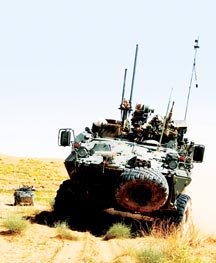
High-performance receiver manufacturers who design products for high-dynamic or high-vibration environments (see cover) where the contribution of phase noise from the local oscillator to velocity error cannot be ignored. In these areas, the strategy outlined here would produce equipment that can perform to higher specifications with the same or a lower-cost oscillator.
The trade-off requires two tracking channels per satellite signal, but this should not pose a problem. At ION GNSS 2009, manufacturers showed receivers with 226 tracking channels. There are currently only 75 live signals in the sky, including all of GPSL1/L2/L5 and GLONASS L1/L2. — Gérard Lachapelle
If the channel data within a GNSS receiver is handled in an effective manner, it is possible to form meaningful estimates of the local-oscillator phase deviations on timescales of 10 milliseconds (ms) or less. Moreover, if certain criteria are met, these estimates will be available with related uncertainties similar to the deviations produced by a typical oven-controlled crystal oscillator (OCXO). The processing delay required to form this estimate is limited to between 10 and 20 ms. In short, it becomes possible in near-real-time to remove the majority of the phase noise of a local oscillator that possesses short-term instability worse than an OCXO, using standalone GNSS. This represents both a new method to accurately determine the Allan deviation of a local oscillator at time scales previously impractical to assess using a conventional GNSS receiver, and the potential for the reduction in observable Doppler uncertainty at the output of the receiver, as well as ionospheric scintillation detection not reliant on an expensive local OCXO.
Concept. Inside a typical GNSS receiver, the estimate of the error in the local oscillator is formed as a component of the navigation solution, which is in turn based on the output of each satellite-tracking channel propagating its estimate of carrier and code measurements to a common future point. While this method of ensuring simultaneous measurements is necessary, it regrettably limits the resolution with which the noise of the local oscillator can be quantified, due to the scaling of non-simultaneous samples of local oscillator noise through the measurement propagation process. To bypass these shortcomings requires a method of coherently gathering information about the phase change in the local oscillator across all available satellite signals: to use the same samples simultaneously for all satellites in view to estimate the center-point phase error common across the visible constellation.
To explain how this is feasible, we must first understand the limitations imposed by the conventional receiver architecture, with respect to accurately estimating short-term oscillator behavior, and subsequently to determine the potential pitfalls of the proposed modifications, including processing delays needed for bit wipe-off, expected observation noise, and user dynamics effects.
Typical Receiver Shortfalls
In a typical receiver, while information about local time offset and local oscillator frequency bias may be recovered, information about phase noise in the local oscillator is distorted and discarded, as a consequence of scaling non-simultaneous observations to a common epoch.
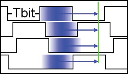
As shown in FIGURE 1, coherent summation intervals in a receiver are used to approximate values of the phase error, including oscillator phase, measured at the non-simultaneous interval centrers in each channel, which are then propagated to a common navigation solution epoch. Each channel will intrinsically contain a partially overlapping midpoint estimate of oscillator noise over the coherent summation interval that will then be scaled by the process of extrapolation. As these estimates are scaled and partially overlapping, they do not make optimal use of the information known about the effects of the local oscillator, and form a poor basis for estimating the contributions of this device to the uncertainty in the channel measurements. As shown in Figure 1, the phase error measured in each channel will be distorted by an over unity scaling factor.
FIGURE 1. Propagation and scaling of phase estimates within a typical receiver.
Depending on implementation decisions made by the designers of a given GNSS system, the average value of the propagation interval relative to the bit period will have different expected values. Assuming the destination epoch is the immediate end of the furthest advanced (most delayed) satellite bitstream, and that integration is carried out over full bit periods, the minimum propagation interval for this satellite would be ½-bit period.
For the average satellite however, the propagation delay would be this ½-bit period plus the mean skew between the furthest satellite and the bitstreams of other space vehicles. Ignoring further skew effects due to the clock errors within the satellites, which are typically limited well below the ms level, the skew between highest and lowest elevation GPS satellites for a user on the surface of earth would be approximately 10 ms. The average value of this skew due to ranging change over orbit, assuming an even distribution of satellites in the sky at different elevation angles, would therefore be 5 ms.
Combining the minimum value of the skew interval with the minimum propagation interval of the most delayed satellite yields a total average propagation interval of 15 ms. In turn, this gives a typical scaling factor of 1.75, used from this point forward when referring to the effects of scaling this quantity.
Proposed Implementation
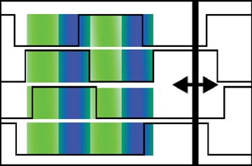
Overcoming limitations of a typical receiver requires recording the approximate bit-timing and history of each tracked satellite as well as a short segment of past samples. This retained data guarantees that the bit-period boundaries of the satellites will not pose an obstacle to forming common N-ms coherent periods between all visible satellites, over which simultaneous integration may proceed by wiping off bit transitions. Using this approach as shown in FIGURE 2, all available constellation signal power is used to estimate a single parameter, namely the epoch-to-epoch phase change in the local oscillator.
FIGURE 2. Common intervals over which to accurately estimate local oscillator phase changes.
Having viewed the existence of these common periods, it becomes evident that it is conceptually possible to form time-synchronized estimates of the phase contribution of the common system oscillator alternately across one N-ms time slice, then the next, in turn forming an unb
roken time series of estimates of the phase change of the system oscillator. Forming the difference between the adjacent discriminator outputs will provide the following information:
The ΔEps (change in the noise term in the local loop)
The ΔOsc (change in the phase of the local oscillator, the parameter of interest)
The ΔDyn (change in the untracked/residual of real and apparent dynamics of the local loop/estimator)
Noticing that term 1 may be considered entirely independent across independent PRNs (GPS, Galileo, Compass) or frequency channels (GLONASS), and that the value of term 3 over a 10-ms period is expected to be small over these short intervals, it becomes obvious that term 2 can be recovered from the available information. To determine the weighting for each satellite channel, the variance of the output of the discriminator is needed.
Performance Determination
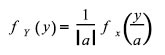
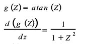
To allow the realistic weighting of discriminator output deltas, it becomes desirable to estimate at very short time intervals the variance of the output of the phase discriminator. In the case of a 2-quadrant arctangent discriminator, this means one wishes to quantify the variance
Letting Q/I 5 Z, recall that if Y 5 aX then
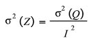
Applying this to the variance of the input to the arctangent discriminator in terms of the in phase and quadrature accumulators, this would give
Rather than proceed with a direct evaluation from this point onward to determine the expression for the variance at the output of the discriminator, it is convenient to recognize that simpler alternatives exist since
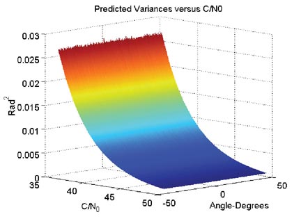
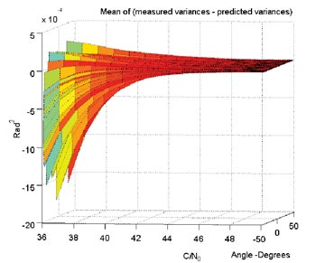
The implication is that since the slope of the arctangent transfer function is very nearly equal to 1 in the central, typical operating region, and universally less than 1 outside of this region, it is easy to recognize that the variance at the output of the arctangent discriminator is universally less than that at the input, and can be pessimistically quantified as the variance of the input, or σ2(Z). This assumption has been verified by simulation, its result shown in FIGURE 3, where the response has been shown after taking into account the effect of operating at a point anywhere in the range ±45 degrees. While the consequence of the simplification of the variance expression is an exaggeration of discriminator output variance, FIGURE 4 shows output variance is well bounded by the estimate, and within a small margin of error for strong signals.
FIGURE 3. Predicted variances at the output of the ATAN2 discriminator versus C/N0.FIGURE 4. Difference between actual and predicted variance at output of discriminator.
The gap between real and predicted output variance may also be narrowed in cases where Q>I by using a type of discriminator which interchanges Q and I in this case and adds an appropriate angular offset to the output as
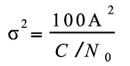
Proceeding in this vein, the next required parameter is the normalized variance of the in-phase and quadrature arms.
The carrier amplitude A can be roughly approximated as
Resulting in a carrier power C
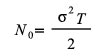
Further, the noise power is given as
Expressing bandwidth B as the inverse of the coherent integration time, and rearranging now gives noise density N0 as
Combining this expression, and the one previously given for the carrier power C results in the following expression for the carrier to noise density ratio:
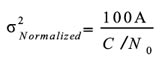
This latest expression can be rearranged to find the desired variance term. Assuming the 10-ms coherent integration time discussed earlier is used, this yields
Normalizing for the carrier amplitude gives the normalized variance in terms of radians squared:
In any situation where the carrier is sufficiently strong to be tracked, it is likely that the carrier power term employed above can be gathered from the immediate I and Q values, ignoring the contribution of the noise term to its magnitude.
Oscillator Phase Effect. Determining the expected magnitude of the local oscillator phase deviation requires only three steps, assuming that certain criteria can be met. The first requirement is that the averaging times in question must be short relative to the duration, at which processes other than white phase and flicker phase modulation begin to dominate the noise characteristics of the oscillator. Typically the crossover point between the dominance of these processes and others is above 1 s in averaging interval length, when quartz oscillators are concerned. Since this article discusses a specific implementation interval of 10 ms within systems expected to be using quartz oscillators, it is reasonable to assume that this constraint will be met.
The second requirement is that the Allan deviation of the given system oscillator must be known for at least one averaging interval within the region of interest. Since the Allan deviation follows a linear slope of -1 with respect to averaging interval on a log-log scale within the white-phase noise region, this single value will allow an accurate prediction of the Allan deviation at any other point on the interval and, in turn, of the phase uncertainty at the 10 ms averaging interval level.
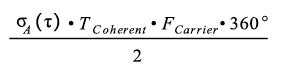
Letting σΔ(τ) represent the Allan deviation at a specific averaging interval, recall that this quantity is the midpoint average of the standard deviation of fractional frequency error over the averaging interval τ. Scaling this quantity by a frequency of interest results in the standard deviation of the absolute frequency error on the averaging interval:
By integrating this average difference in frequency deviations over the coherent period of interest, one obtains a measure of the standard deviation in degrees, of a signal generated by this reference:
Note that the averaging interval τ must be identical to the coherent integration time.
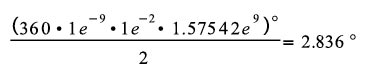
Turning to a practical example, if the oscillator in question has a 1 s Allan Deviation of 1 part per hundred billion (1 in 1011), a stability value between that of an OCXO and microcomputer compensated crystal oscillator (MCXO) standard, and shown to be somewhat pessimistic, this would scale linearly to be 1e-9 at a 10-ms averaging interval, under the previous assumption that the oscillator uncertainty is dominated by the white phase-noise term at these intervals. Also, for illustration purposes, if one assumes the carrier of interest to be the nominal GPS L1 carrier, the uncertainty in the local carrier replica due to the local oscillator over a 10-ms coherent integration time becomes
When stated in a more readily digested format, this represents roughly 15 centimeter/second in the line-of-sight velocity uncertainty. In an operating receiver, two additional factors modify this effect. The first is the previously discussed scaling effect that will tend to exaggerate this effect by a typical factor of 1.75, as previously discussed. The second factor is that this noise contribution is filtered by the bandwidth-limiting effects of the local loop filter, producing a modification to the noise affecting velocity estimates, as well as reduced information about the behaviour of the local oscillator.
Impact of Apparent Dynamics. When considering the error sources within the system, it is important to realize which individual sources of error will contribute to estimation errors, and which will not. One area of potential concern would appear to be the errors in the satellite ephemerides, encompassing both the satellite-orbit trajectory misrepresentation and the satellite clock error. While the errors in the satellite ephemerides are of concern for point positioning, they are not of consequence to this application, as the apparent error introduced by a deviation of the true orbit from that expressed in the broadcast orbital parameters does not affect the tracking of that satellite at the loop level.
Additionally, while the satellite clock will add uncertainty to the epoch-to-epoch phase change within each channel independently, the magnitude of this change is minimal relative to the contribution of uncertainty due to the variance at the output of the discriminator guaranteed by the low carrier-to-noise density ratio of a received GNSS signal. Since this contribution is uncorrelated between satellites and relatively small compared to other noise contributions affecting these measurements, even when compared to the soon-to-be-discontinued Uragan GLONASS satellites that had generally less stable onboard clocks, it is likely safe to ignore. When compared to the more stable oscillators aboard GPS or GLONASS-M satellites, it is a reasonable assumption that this will be a dismissible contribution to received signal-phase uncertainty change.
While atmospheric effects present an obstacle which will directly affect the epoch-to-epoch output of the discriminators, it is believed that under conditions that do not include the effects of ionospheric scintillation the majority of the contribution of apparent dynamics due to atmospheric changes will have a power spectral density (PSD) heavily concentrated below a fraction of 1 Hz. The consequence of this concentration is that the tracking loops will remove the vast majority of this contribution, and that the difference operator that will be applied between adjacent phase measurements, as in the case of dynamics, will nullify the majority of the remaining influence.
Impact of Real Dynamics. Real dynamics present constraints on performance, as do any tracking loop transients. For example, a low-bandwidth loop-tracking dynamics will have long-lasting transients of a magnitude significant relative to levels of local oscillator noise. For this reason it is necessary to adopt a strategy of using the epoch-to-epoch change in the discriminator as the figure of interest, as opposed to the absolute error-value output at each epoch. This can reasonably be expected to remove the vast majority of the effects of dynamics of the user on the solution.
To validate this assumption under typical conditions calls for a short verification example. Assuming the use of a second-order phase-locked loop (PLL) for carrier tracking, with a 10-Hz loop bandwidth the effects of dynamics on the loop are given by these equations:
Letting Bn be 10 Hz, one can write
Recall that the dynamic tracking error in a second-order tracking loop is given by
Given the choices above, this would result in a constant offset of 0.00281 cycles, or 1.011 degrees of constant tracking error due to dynamics, following from the relation between line-of-sight acceleration and loop bandwidth to tracking error. Since this constant bias will be eliminated by the difference operator discussed earlier, it is necessary to examine higher order dynamics.
Further, if one used a coherent integration interval of 10 ms as assumed earlier, and let the dynamics of interest be a jerk of 1 g/s, this results in a midpoint average of 0.005 g on this interval:
Substituting this result into equation 16 produces the associated change in dynamic error over the integration interval, which is in this case:
This value will be kept in mind when evaluating capabilities of the estimation approach to determine when it will be of consequence. As the estimation process will be run after a short delay, an existing estimate of platform dynamics could form the basis of a smoothing strategy to reduce this dynamic contribution further.
Estimated Capabilities
In the absence of the influence of any unmodeled effects, the expected performance of this method is dependent on only the number of satellite observables and their respective C/N0 ratios. Across each of these scenarios we assume for simplicity’s sake that each satellite in view is received at a common C/N0 ratio and over a common integration period of 10 ms.
If the assumption of minimal dynamic influences is met, the situation at hand becomes one in which multiple measures of a single quantity are present, each containing independent (due to CDMA or FDMA channel separation) noise influences with a nearly zero mean. When one can express the available data form:
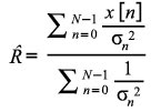
x[n] = R + w[n]
where x[n] is the nth channel discriminator delta which includes the desired measure of the local oscillator delta (R), as well as w[n], a strong, nearly white-noise component, there are multiple approaches for the estimation of R.
The straightforward solution to estimate R in this case is to use the predicted variances of each measure to serve as an inverse weighting to the contribution of each individual term, followed by normalization by the total variance, as expressed by
Now, since it is desired to bound the uncertainty of the estimate of R, the variance of this quantity should also be noted. This uncertainty can be determined as
To determine the performance of the estimation method for a given constellation configuration, with specific power levels and available carrier signals, it is necessary to utilize the predicted variances plotted in Figure 3 as inputs to equations 20 and 21. To provide numerical examples of the performance of this method, three scenarios span the expected range of performance.
Scenario 1 is intended to be char-acteristic of that visible to a single-freq-uency GPS user under slight attenuation. It is assumed that 12 single-frequency satellites are visible at a common C/N0 of 36 dB-Hz, yielding from the simulation curves a value for each channel of 0.0265 rad2. When substituted into equation 24, this predicts an estimation uncertainty of
This is a level of estimation uncertainty similar to that assumed to be intrinsic to the local oscillator in the previous section. The result implies that with this minimally powerful set of satellites, it becomes possible to quantify the behavior of the local oscillator with a level of uncertainty commensurate with the actual uncertainty in the oscillator over the 10 ms averaging interval.
Consequentially, this indicates that the Allan deviation of this system oscillator could be wholly evaluated under these conditions at any interval of 10 ms or longer. Further, if the system oscillator were in fact the less stable MCXO from the resource above, this estimate uncertainty would be significantly lower than the actual uncertainty intrinsic to the oscillator, providing an opportunity to “clean” the velocity measurements.
Scenario 2 is intended to be characteristic of a near future multi-constellation single-frequency receiver. It is assumed that eight satellites from three constellations are visible on a single frequency each, with a common C/N0 of 42 dB-Hz, yielding a value for each channel of 6.4e-3 rad2, leading to an estimation uncertainty of
Scenario 3 is intended to serve as an optimistic scenario involving a future multi-frequency, multi-constellation receiver. It is assumed that nine future satellites are available from each of three constellations, each with four independent carriers, all received at 45 dB-Hz, yielding a value for each channel of 3.2e-3 rad2, leading to an estimation uncertainty of
Application to Observations
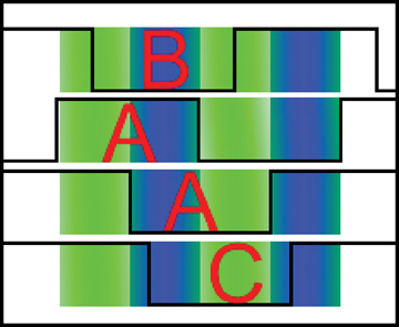
The theoretical benefit of subtracting these phase changes from the measurements of an individual loop prior to propagating that measurement to the common position solution epoch ranges from moderate to very high depending on the satellite timing skew relative to the solution point. The most beneficial scenario is total elimination of oscillator noise effects (within the uncertainty of the estimate), which is experienced in the special case (Case A, FIGURE 5), where the bit period of a given satellite falls entirely over two of the 10-ms subsections. The uncertainty would increase to 2x the level of uncertainty in the estimate in the special case (Case B) where the satellite bit period straddles one full 10-ms period and two 5-ms halves of adjacent periods, and would lie somewhere between 1 and 2 times the level of uncertainty for the general case where three subintervals are covered, yet the bit period is not centered (Case C).
FIGURE 5. Special cases of oscillator estimate versus bit-period alignment.
While the application to observations of the predicted oscillator phase changes between integration intervals does not appear immediately useful for high-end receiver users with the exception of those in high-vibration or scintillation-detection applications, it could be applied to consumer-grade receivers to facilitate the use of inexpensive system clocks while providing observables with error levels as low as those provided by much more expensive receivers incorporating ovenized frequency references.
Further Points
While the chosen coherent integration period may be lengthened to increase the certainty of the measurement from a noise averaging perspective, this modification risks degrading the usefulness of said measurement due to dynamics sensitivities. Additionally, as the coherent integration time is increased, the granularity with which the pre-propagation oscillator contribution may be removed from an individual loop will be reduced. While this may be useful in cases of very low dynamics where the system is intended to estimate phase errors in a local oscillator with high certainty, it would be of little use if one desires to provide low-noise observables at the output.
For this reason, it is recommended that increases in coherent integration time be approached with caution, and extra thought be given to use of dynamics estimation techniques such as smoothing, via use of the subsequent n-ms segment in the formation of the estimate of dynamics for the “current” segment. This carries the penalty of increased processing latency, but could greatly reduce dynamics effects by enabling their more reliable excision from the desired phase-delta measurements.
Acknowledgments
The author thanks his supervisors, Gerard Lachapelle and Elizabeth Cannon, and the Natural Sciences and Engineering Research Council of Canada, the Alberta Informatics Circle of Research Excellence, the Canadian Northern Studies Trust, the Association of Canadian Universities for Northern Studies, and Environment Canada for financial and logistical support.
AIDEN MORRISON is a Ph.D. candidate in the Position, Location, and Navigation (PLAN) Group, Department of Geomatics Engineering, Schulich School of Engineering at the University of Calgary, where he has developed a software-defined GPS/GLONASS receiver for his research.
GPS receivers must deal with measurements and models that have some degree of error, which gets propagated into the position solution. If the errors are systematically different for the different simultaneous pseudoranges, as is typically the case when trying to correct for ionospheric and tropospheric effects, these errors propagate into the receiver solution in a way that is fundamentally different from the way that random errors propagate. So in addition to dilution of precision, we need a companion measure of systematic effects. In this month’s column, we introduce just such a measure.
INNOVATION INSIGHTS by Richard Langley
WE LIVE IN AN IMPERFECT WORLD. We know this all too well from life’s everyday trials and tribulations. But this statement extends to the world of GPS and other global navigation satellite systems, too. A GPS receiver computes its three-dimensional position coordinates and its clock offset from four or more simultaneous pseudoranges. These are measurements of the biased range (hence the term pseudorange) between the receiver’s antenna and the antenna of each of the satellites being tracked. The receiver processes these measurements together with a model describing the satellite orbits and clocks and other effects, such as those of the atmosphere, to determine its position. The precision and accuracy of the measured pseudoranges and the fidelity of the model determine, in part, the overall precision and accuracy of the receiver-derived coordinates.
If we lived in an ideal world, a receiver could make perfect measurements and model them exactly. Then, we would only need measurements to any four satellites to determine our position perfectly. Unfortunately, the receiver must deal with measurements and models that have some degree of error, which gets propagated into the position solution. Furthermore, the geometrical arrangement of the satellites observed by the receiver — their elevation angles and azimuths — can significantly affect the precision and accuracy of the receiver’s solution, typically degrading them. It is common to express the degradation or dilution by dilution of precision (DOP) factors. Multiplying the measurement and model uncertainty by an appropriate DOP value gives an estimate of the position error.
These estimates are reasonable if the measurement and model errors are truly random. However, it turns out that this simple geometrical relationship breaks down if some model errors are systematic. If that systematic error is a constant bias and if it is common to all pseudoranges measured simultaneously, then the receiver can easily estimate it along with its clock offset, leaving the position solution unaffected. But if the errors are systematically different for the different simultaneous pseudoranges, as is typically the case when trying to correct for ionospheric and tropospheric effects, these errors propagate into the receiver solution in a way that is fundamentally different from the way that random errors propagate. This means that in addition to DOP, we need a companion measure of systematic effects.
In this month’s column, Dennis Milbert introduces just such a measure — the error scale factor or ESF. ESF, combined with DOP, forms a hybrid error model that appears to more realistically portray the real-world GPS precisions and accuracies we actually experience.
“Innovation” features discussions about advances in GPS technology, its applications, and the fundamentals of GPS positioning. The column is coordinated by Richard Langley, Department of Geodesy and Geomatics Engineering, University of New Brunswick.
The recent edition of the Standard Positioning Service (SPS) Performance Standard (PS) and the corresponding document for the Precise Positioning Service (PPS) both emphasize a key element. They only specify the GPS signal-in-space (SIS) performance. Since these standards do not define performance for any application of a GPS signal, it becomes even more important to understand the relationship of signal statistics to positioning accuracy. Historically, as well as in Appendix B of the SPS-PS and PPS-PS, this relationship is modeled by covariance elements called dilution of precision (DOP).
Many references are available which describe DOP. The core of DOP is the equation of random error propagation:
Qx= ( AtQ-1A ) -1
where, for n observations, A is the n x 4 matrix of observation equation partial differentials, Q is the n x n covariance matrix of observations, and Qx is the 4 x 4 covariance matrix of position and time parameters (X, Y, Z, T) used to compute DOPs. This equation describes the propagation of random error (noise) in measurements into the noise of the unknown (solved for) parameters. Elements of the Qx matrix are then used to form the DOP.
The equation above is linear for any measurement scale factor of Q. For example, halving the dispersion of the measurements will halve the dispersion of the positional error. This scaling behavior is exploited when forming DOP where, by convention, Q is taken as the identity matrix, I. DOPs then become unitless, and are treated as multipliers that convert range error into various forms of positional error. Thus, we see relationships in the SPS-PS Appendix B such as:
UHNE = UERE x HDOP
where UERE is user equivalent range error, HDOP is horizontal dilution of precision, and UHNE is the resulting user horizontal navigation error.
DOP is a model relationship between signal statistics and position statistics based on random error propagation. But, since the cessation of Selective Availability (SA), the GPS signal in space now displays less random dispersion than the average systematic effects of ionosphere and troposphere propagation delay error. It’s useful to test if a random error model can capture the current behavior of GPS positioning on the ground.
The Federal Aviation Administration collects GPS data at the Wide Area Augmentation System (WAAS) reference stations and analyzes GPS SPS performance. These analyses are documented in a quarterly series called the Performance Analysis (PAN) Reports. To test horizontal and vertical accuracy, the 95th percentile of positional error, taken comprehensively over space and time, without any subsetting whatsoever, is chosen. This measure is always found in Figures 5-1 and 5-2 of the PAN reports. Note that the Appendix A 95% “predictable accuracy” in the reports through PAN report number 51 refers to a worst-site condition and cannot be considered comprehensive. The PAN report 95th percentiles of positional error measured since the cessation of SA are reproduced in FIGURE 1.
Figure 1. Accuracy (95th percentile) of horizontal and vertical L1-only point positioning. GPS data are gathered at WAAS reference stations, analyzed quarterly, and published in the PAN reports. The red line is vertical accuracy and the blue line is horizontal accuracy.
By the DOP error model, the positional error should be the product of the underlying pseudorange error times HDOP
or vertical DOP (VDOP). It is convenient to form the vertical to horizontal positional error ratio, V/H, shown in FIGURE 2. This error ratio should, formally, be independent of the magnitude of the range error. The error ratio should reflect the GPS constellation geometry. One expects the positional error ratio, V/H, to be relatively uniform, and it should also equal the VDOP/HDOP ratio. However, Figure 2 shows a number of spikes (from PAN Reports 37, 40, 44, 64) in the error ratio, and a general increase over the past nine years. The positional error ratios in Figure 2 do not portray the uniform behavior expected for a DOP error model based on random error propagation.
Figure 2. Ratio of the vertical/horizontal accuracy (95th percentile). The spikes indicate effects that are not caused by constellation geometry or signal-in-space error.
The PAN reports form a challenge to our ability to understand and describe the measured performance of the GPS system. In the past, when SA was imposed on the GPS signal, the measured pseudorange displayed random, albeit time-correlated, statistics. DOP was effective then in relating SA-laden range error to positional error. Now, with SA set to zero, the role of DOP should be revisited.
In this article, I will introduce a hybrid error model that takes into account not only the effects of random error but also that of systematic error due to incomplete or inaccurate modeling of observations. But first, let’s examine predicted GPS performance based on DOP calculations alone.
Random Error Propagation
FIGURE 3 displays detail of a 24-hour HDOP time series. Considerable short wavelength structure is evident. Spikes as thin as 55 seconds duration can be found at higher resolutions. Given the abrupt, second-to-second transitions in DOP, and given that the GPS satellites orbit relative to the Earth at about 4 kilometers per second, one may suspect that short spatial scales as well as short time scales are needed to describe DOP behavior.
Figure 3. All-in-view HDOP, July 20, 2007, near the Washington Monument, 5° elevation angle cutoff. Note the abrupt transitions, and that HDOP is around 1.0. VDOP (not pictured) is about 1.5.
To investigate DOP transitions, the conterminous United States (CONUS) was selected as a study area. HDOP and VDOP, with a 5° elevation-angle cutoff, were computed using an almanac on a regular 3 minute by 3 minute grid over the region 24°-53° N, 230°-294° E. These DOP grids were computed at 2,880 30-second epochs for July 20, 2007, yielding more than two trillion DOP evaluations. This fine time/space granularity was selected to capture most of the complex DOP structure seen in Figure 3.
FIGURE 4 plots the HDOP distribution over CONUS and parts of Canada and Mexico at 02:40:30 GPS Time. This epoch was selected to show an HDOP excursion (HDOP 4 2.58) seen in the red zone just north of Lake Ontario. DOPs are rather uniform within zones, and these zones have curved boundaries. The boundaries are sharply delineated and move geographically in time, which explains the jumps seen in high-rate DOP time series (as in Figure 3). The broad, curved boundaries seen in Figure 4 are the edges of the footprints of the various GPS satellites. The gradual variation in hue within a zone shows the gradual variation of DOP as the spatial mappings of the local elevation angles change for a given set of GPS satellites in a region.
Figure 4. HDOP, July 20, 2007, 02:40:30 GPS Time, 5° cutoff. The curved boundaries, which show abrupt transitions in DOP, are the edges of the footprints of various GPS satellites.
The 2,880 color images of HDOP (and VDOP) were converted into an animation that runs 4 minutes and 48 seconds at 10 frames per second. The effect is kaleidoscopic, as the various footprints cycle across one another, and as the zones change color. The footprint boundaries transit across the map in various directions and create a changing set of triangular and quadrilateral zones of fairly uniform DOP. There is no lower limit to temporal or spatial scale of a given DOP zone delimited by three transiting boundaries. The size of a zone can increase or shrink in time. Zones can take a local maximum, a local minimum, or just some intermediate DOP value. And the DOP magnitude in a given zone often changes in time. The animation shows that the DOP maximums are quite infrequent, and the DOPs generally cluster around the low end of the color scale. The animations are available.
To get a quantitative measure of distribution, the HDOPs (and VDOPs) are histogrammed with a bin width of 0.01 in FIGURE 5. Tabulations of various percentiles, computed from the bin counts, are displayed in TABLE 1. HDOP ranges from 0.600 to 2.685 and VDOP ranges from 0.806 to 3.810.
Figure 5. HDOP, July 20, 2007, 5° cutoff. DOP has a strong central tendency and a tail showing rare instances of large DOP. Here HDOP ranges from 0.600 to 2.685.
Chart: GPS World
Since the DOP zone boundaries are related to satellites rising and setting, it is natural to expect a relation to a selected cutoff limit of the elevation angle. As a test, DOP was recomputed with a 15° cutoff limit, and histogrammed with a bin width of 0.01 in FIGURE 6. Tabulations of various percentiles, computed from the bin counts, are displayed in TABLE 2. HDOP ranges from 0.735 to 26.335, and VDOP ranges from 1.045 to 72.648.
Figure 6. HDOP, July 20, 2007, 15° cutoff. DOP is sensitive to cutoff angle. Here HDOP ranges from 0.735 to 26.335. This is a large increase over the HDOP with a 5° cutoff.
The Figures 5 and 6 and Tables 1 and 2 show that DOPs are markedly sensitive to cutoff angles. The histogram tails increase and the maximum DOPs dramatically increase as the cutoff angle is increased. The 95th percentile HDOP increases by about 50 percent when the cutoff angle increases from 5° to 15°. The solutions weaken to some degree and the poorer solutions get much worse. The effect is somewhat greater for VDOP.
One normally considers DOP as a property of the satellite constellation that has a space-time mapping. DOP is seen to strongly depend upon horizon visibility. This is a completely local property that is highly variable throughout the region. Clearly, DOP depends on the antenna site as well as the constellation.
Systematic Error Propagation
It is known that certain error sources in GPS are systematic. Such errors will display different behaviors from random error. For example, the impact of ionosphere and troposphere error on GPS performance has been recognized in the literature (see “Further Reading”). DOP is not successful in modeling systematic effects. A new metric for systematic positional error is needed.
Consider a systematic bias, b, in measured pseudorange, R. One may propagate the bias through the weighted least-squares adjustment:
(AtQ-1A) x =AtQ-1y
by setting the n x 1 vector, y = b. Vector x will then contain the differential change (error) in coordinates (δx, δy, δz, δt) induced by the bias. The coordinate rror can then be transformed into the north, east, and up local horizon system (δN, δE, δU). Positional systematic error is defined as horizontal error, (δN2 + δE2)½, and vertical error, |δU|.
As with DOP, the equations above are linear for any measurement bias scale factor, k, which applies to all satellite pseudoranges at an epoch. For example, if one halves a bias that applies to all pseudoranges (for example, ky), then one will halve the associated coordinate error, kx. Analogous to DOP, we take bias with a base error b = 1, to create a unitless measure that can be treated as a multiplier. We now designate the horizontal error as horizontal error scale factor (HESF) and vertical error as vertical error scale factor (VESF). This adds a capability of developing error budgets for systematic effects that parallels DOP.
Systematic errors in GPS position solutions have a distinctly different behavior than random errors. This is illustrated by a trivial example. If one repeats any of the tests above with a constant value, c, for the bias, one will find that, aside from computer round-off error, no systematic error propagates into the position. The coordinates are recovered perfectly, and the constant bias is absorbed into the receiver time bias parameter, δ t. This is no surprise, since the GPS point position model is constructed to solve for a constant receiver clock bias.
The ionosphere and troposphere, on the other hand, cause unequal systematic errors in pseudoranges. These systematic errors are greater for lower elevation angle satellites than for higher elevation angle satellites. So, unlike the trivial example above, these errors cannot be perfectly absorbed into δ t. The systematic errors never vanish, even for satellites at zenith. One may expect some nonzero positional error that does not behave randomly.
The systematic effect of the ionosphere and troposphere differ through their mapping functions. These are functions of elevation angle, E, and are scale factors to the systematic effect at zenith (E = 90°). Because of the different altitudes of the atmospheric layers, the mapping functions take different forms. For this reason, systematic error scale factors (ESFs) for the ionosphere and troposphere must be considered separately.
Ionosphere Error Scale Factor. Following Figure 20-4 of the Navstar GPS Space Segment/Navigation User Interfaces document, IS-GPS-200D, the ionospheric mapping function associated with the broadcast navigation message, F, is
F = 1.0 + 16.0 (0.53 – E)3
where E is in semicircles and where semicircles are angular units of 180 degrees and of π radians. Since the base error is considered to be b = 1 for ESFs, y is simply populated with the various values of F appropriate to the elevation angles, E, of the various satellites visible at a given epoch. The resulting HESF and VESF values will portray how systematic ionosphere error will be magnified into positional error, just as DOPs portray how random pseudorange error is magnified into positional error.
As was done with the DOPs, more than two trillion ionosphere HESFs (and VESFs) were computed for CONUS and histogrammed in FIGURE 7. Tabulations of various percentiles, computed from the bin counts, are displayed in TABLE 3. Ionosphere HESF ranges from 0.0 to 0.440 and VESF ranges from 1.507 to 2.765.
Figure 7. HESF, ionosphere, July 20, 2007, 5° cutoff. The HESF-I are much smaller than the HDOP. The VESF-I (not depicted) have an average larger magnitude than the VDOP.
The distribution of the HESF-I in Figure 7 differs profoundly from HDOP. Ionosphere error is seen to have a weak mapping into horizontal positional error, with HESF-I values approaching zero, and having a long tail. The VESF-I is roughly comparable to the magnitude of the ionosphere mapping function at a low elevation angle. The VESFs also fall into a fixed range, without long tails, and are skewed to the right. The percentiles in Table 3 show ionosphere error has a greater influence on the height than that predicted by DOP.
Systematic Range Error and Height. Both troposphere and ionosphere propagation error leads to error in height. The mechanism underlying the behavior in Table 3 is not obvious. Consider the simplified positioning problem in FIGURE 8, where we solve for two unknowns: the up-component of position and receiver bias, dt (which includes effects common to all pseudoranges measured at the same time, such as the receiver clock offset). The atmosphere will cause the pseudoranges AO, BO, and CO to measure systematically longer. However, the ionosphere error will be about three times larger at low elevation angles than at the zenith. (Troposphere error will be about 10 times larger at low elevation angles than at the zenith.)
Figure 8. Schematic of pseudorange positioning. Computing up and receiver clock bias through 3 pseudoranges (AO, BO, CO), BO is biased by +5 meters ionosphere; AO and CO are biased by +15 meters ionosphere. Clock bias will absorb the +15 meters from the conflicting horizontal pseudoranges, and overcorrect the BO pseudorange by 10 meters.
In this simplified example, assume the zenith pseudorange, BO, measures 5 meters too long because of unmodeled ionosphere delay. Then the near-horizon pseudoranges, AO and CO, will measure 15 meters too long. AO and CO can’t both be 15 meters too long at the same time, so that bias is absorbed by the receiver bias term, dt. That dt term is also a component of the up solution from BO. While the AO and CO pseudoranges have superb geometry in establishing receiver clock bias, they also have terrible geometry in establishing height. The height is solved from the BO pseudorange that is overcorrected by 10 meters. Point O rises by 10 meters. The presence of the receiver bias term causes atmospheric systematic error to be transferred to the height. It also shows that the horizontal error will largely be canceled in mid-latitude and equatorial scenarios.
Troposphere Error Scale Factor. A variety of troposphere models and mapping functions are available in the literature. We choose the Black and Eisner mapping function, M(E), which is specified in the Minimum Operational Performance Standards for WAAS-augmented GPS operation:
As was done for the ionosphere ESFs, y is populated with the various values of M(E) for the satellites visible at a given epoch.
The troposphere HESFs (and VESFs) are computed for CONUS and histogrammed in FIGURE 9. Tabulations of various percentiles, computed from the bin counts, are displayed in TABLE 4. Troposphere HESF ranges from 0.0 to 5.203, and VESF ranges from 1.882 to 13.689.
Figure 9. HESF, troposphere, July 20, 2007, 5° cutoff. The HESF-Ts are significantly larger than the HESF-Is, showing that unmodeled troposphere propagation error can more readily influence horizontal position. The VESF-Ts are substantially larger than the VDOPs and VESF-Is.
The troposphere HESFs in Table 4 have similarities with, and differences from, the ionosphere HESFs of Table 3. Troposphere error maps more strongly into the horizontal coordinates than ionosphere error. The VESFs are much larger than the HESFs. And the VESFs still fall into a fixed range, without long tails.
Unlike DOP, which is derived from random error propagation, ESF is constructed for systematic error propagation. A good “vest pocket” number for the tropospheric delay of pseudorange at zenith is 2.4 meters at mean sea level. Thus, without a troposphere model, one can expect horizontal error of 1.80 x 2.4 meters = 4.32 meters or less 95 percent of the time according to Table 4.
Cutoff Angle. We now briefly consider the behavior of ESF under an increased elevation angle cutoff. The ionosphere ESFs with a 10° cutoff show minor improvements. This is a distinct difference from DOP (see Table 2), which showed degraded precision with a larger cutoff angle. The troposphere ESFs with a 10° cutoff angle are computed from histogram bin counts (TABLE 5). 10° cutoff troposphere HESF ranges from 0.0 to 3.228 and VESF ranges from 1.161 to 9.192.
Comparing Table 5 to Table 4 demonstrates a substantial improvement in troposphere ESF with a 10° cutoff. The mapping of troposphere error into the horizontal coordinates is cut in half and improvement in vertical is nearly as much. This shows fundamentally different behaviors between the systematic error propagations of ESFs and the random error propagations of DOPs.
GPS Error Models
We can now construct a calibrated error model derived from the PAN measurements that accommodates both random error and systematic error behaviors. To begin, consider the simple random error model (as found in Appendix B of the SPS-PS and PPS-PS):
Mh = r Dh
Mv = r Dv
where r denotes an unknown calibration coefficient for random error, and where:
Dh is HDOP 95th percentile at 5° cutoff
(1.24 by Table 1)
Dv is VDOP 95th percentile at 5° cutoff (1.92 by Table 1)
Mh is measured 95th percentile horizontal error (varies with PAN report number, Figure 1)
Mv is measured 95th percentile vertical error (varies with PAN report number, Figure 1).
One immediately sees by inspection that we have not one, but two estimates of r for each PAN report. And these estimates are inconsistent.
Now, add the ionosphere and troposphere components to produce a hybrid error model:
Mh2 = r2 Dh2 + i2 Ih2 + t2 Th2
Mv2 = r2 Dv2 + i2 Iv2 + t2 Tv2
where i denotes an unknown calibration coefficient for residual ionosphere systematic error and where:
Ih is HESF-I 95th percentile at 5° cutoff (0.162 by Table 3)
Iv is VESF-I 95th percentile at 5° cutoff (2.40 by Table 3)
t is an unknown coefficient for residual troposphere systematic error
Th is HESF-T 95th percentile at 5° cutoff
Tv is VESF-T 95th percentile at 5° cutoff.
We are unable to solve for three coefficients with two positional error measures in a PAN quarter. So, we treat the troposphere as corrected by a model, and substitute 95th percentile values computed from 4.9 centimeters of residual troposphere error:
Mh2 = r2 Dh2 + i2 Ih2 + (0.01)2
Mv2 = r2 Dv2 + i2 Iv2 + (0.60)2
This leads to a 2 x 2 linear system for each PAN quarter. The r and i coefficients are solved for and displayed in FIGURE 10.
Figure 10. Hybrid model of random and ionosphere error by PAN report number. Red line is random error; blue line is ionosphere. Gaps in the plot indicate inconsistent coefficient solutions.
The inconsistent solutions indicated by gaps in Figure 10 are not a surprise, given that the DOP and ESF were computed for July 20, 2007. Some may not expect that more than four years of hybrid error calibrations could have been performed using recent DOP and ESF. Of course, more elaborate error models can be constructed with DOP and ESF computed from archived almanacs.
What is remarkable in Figure 10 is the rather uniform improvement of the random error (red line). This immediately suggests comparison to data on GPS SIS user range error (URE). Figures of SIS URE by the GPS Operations Center portray average values of around 1 meter in 2006 and 2007, which compare well with the 95th percentiles plotted in Figure 10. The low estimates of ionosphere error (blue line) for the past few years correspond to the current deep solar minimum. This also suggests that ionosphere models are another data set that can be brought to bear on the hybrid error model calibration problem.
This hybrid error model is just a first attempt at simultaneously reconciling random and systematic effects. It shows some capability to distinguish ionosphere error from other truly random noise sources. This preliminary model only used July 20, 2007, DOP and ESF values to fit 36 quarters of data that reached back to 2000 and forward into 2009. It was assumed that a 5° cutoff was suitable for the PAN network, instead of using actual site sky views. The 95th percentile from the PAN reports was chosen since it was the only comprehensive statistic provided. A 50th percentile, if it had been available, is a more robust statistic.
Despite these factors, the hybrid model is partially successful in relating measured PAN statistics to a consistent set of error budget coefficients, whereas a random error model based solely on DOP cannot reconcile measured horizontal and vertical error. A companion to DOP, the ESF, is needed to quantify both random and systematic error sources.
Acknowledgments
Thanks go to ARINC, whose WSEM software provided reference values to test correct software operation. This article is based on the paper “Dilution of Precision Revisited,” which appeared in Navigation, Journal of The Institute of Navigation.
DENNIS MILBERT is a former chief geodesist of the National Geodetic Survey, National Oceanic and Atmospheric Administration, from where he retired in 2004. He has a Ph.D. from The Ohio State University. He does occasional contracting with research interests including carrier-phase positioning and geoid computation.
FURTHER READING
• Dilution Of Precision
“Dilution of Precision Revisited” by D. Milbert in Navigation, Journal of The Institute of Navigation, Vol. 55, No. 1, 2008, pp. 67–81.
“Dilution of Precision” by R.B. Langley in GPS World, Vol. 10, No. 5, May 1999, pp. 52–59.
“Satellite Constellation and Geometric Dilution of Precision” by J.J. Spilker Jr. and “GPS Error Analysis” by B.W. Parkinson in Global Positioning System: Theory and Applications, Vol. 1, edited by B.W. Parkinson and J.J. Spilker Jr., Progress in Astronautics and Aeronautics, Vol. 163, American Institute of Aeronautics and Astronautics, Washington, D.C., 1996, pp. 177–208 and 469–483.
“Post-Modernization GPS Performance Capabilities” by K.D. McDonald and C.J. Hegarty in Proceedings of the IAIN World Congress and the 56th Annual Meeting of The Institute of Navigation, San Diego, California, June 26–28, 2000, pp. 242–249.
“The Residual Tropospheric Propagation Delay: How Bad Can It Get?” by J.P. Collins and R.B. Langley in Proceedings of ION GPS-98, 11th International Technical Meeting of the Satellite Division of The Institute of Navigation, Nashville, Tennessee, September 15–18, 1998, pp. 729–738.
“The Role of the Clock in a GPS Receiver” by P.N. Misra in GPS World, Vol. 7, No. 4, April 1996, pp. 60–66.
“The Effects of Ionospheric Errors on Single-Frequency GPS Users” by R.L. Greenspan, A.K. Tet[e]wsky, J. I. Donna, and J.A. Klobuchar in ION GPS 1991, Proceedings of the 4th International Technical Meeting of the Satellite Division of the Institute of Navigation, Albuquerque, New Mexico, September 11–13, 1991, pp. 291–298.
• GPS Standards and Specifications
Global Positioning System Standard Positioning Service Performance Standard, U.S. Department of Defense, Washington, D.C., September 2008.
Global Positioning System Precise Positioning Service Performance Standard, U.S. Department of Defense, Washington, D.C., February 2007.
Navstar Global Positioning System Interface Specification, IS-GPS-200D, Revision D, IRN-200D-001, by ARINC Engineering Services, LLC for GPS Joint Program Office, El Segundo, California, March 2006.
 Learning about the latest tools and techniques is the primary reason for conferences, and there is agreement in the geospatial community that GEOINT is the place to be. Organized by the United States Geospatial Intelligence Foundation (USGIF), attendance at the San Antonio conference was the highest it has ever been, according to USGIF President Keith Masback. Even with a weak economy, the over-arching opinion of all attendees was that the intelligence business will continue to grow regardless of world politics. By its nature, this conference really had many more “chiefs” than “Indians,” and many exhibitors spared no expense at the conference, knowing that they were reaching key decision makers.


 Four Galileo in-orbit validation (IOV) satellites scheduled to launch next year have already missed their first pad date.The European version of Russia’s Soyuz rocket is now scheduled to carry the four IOV satellites into orbit in two launches in November 2010 and early 2011, as announced by European Space Agency (ESA) Director-General Jean-Jacques Dordain on October 9.