Blog

  • Innovation: How Deep Is That White Stuff?

    Innovation: How Deep Is That White Stuff?

    Using GPS Multipath for Snow-Depth Estimation

    By Felipe G. Nievinski and Kristine M. Larson

    INNOVATION INSIGHTS by Richard Langley
    INNOVATION INSIGHTS by Richard Langley

    FRINGES. No, I’m not talking about the latest celebrity hairstyles nor the canopy of an American doorless, four-wheeled carriage from yesteryear (think Oklahoma!). I’m talking about interference fringes. But there is a connection to these other uses of the word fringe as we’ll see. You’ve all seen interference fringes at your local gas station, typically after it has just rained. They are the alternating bands of color we perceive when looking at a gasoline or oil slick in a puddle of water. They are caused by the white light from the Sun or artificial lighting reflected from the top surface of the slick and that from the bottom surface at the slick-water interface combining or interfering with each other at our eyeballs. The two sets of light waves arrive slightly out of phase with each other, and depending on the wavelengths of the reflected light and our angle of view, produce the colorful fringes. If the incident light was monochromatic, consisting of a single frequency or wavelength, then we would perceive just alternating bright and dark bands. The bright bands result from constructive interference when the phase difference is a near a multiple of 2π whereas the dark bands result from destructive interference when the difference is near an odd multiple of π.

    Interference fringes had been seen long before the invention of the automobile. They are clearly seen on soap bubbles and the iridescent colors of peacock feathers, Morpho butterflies, and jewel beetles are also due to the interference phenomenon rather than pigmentation. Sir Isaac Newton did experiments on interference fringes (amongst other things) and tried to explain their existence — wrongly, it turned out. But he did coin the term fringes since they resembled the decorative fringe sometimes used on clothing, drapery, and, yes, surrey canopies.

    It was the English polymath, Thomas Young, who, in 1801, first demonstrated interference as a consequence of the wave-nature of light with his famous double-slit experiment. You may have replicated his experiment in a high-school physics class. I did and I think I did it again as an undergraduate student taking a course in optics. Already by that point I was aiming for a career in physics or space science but I didn’t know that as a graduate student I would do research involving interference fringes. But not using light waves.

    My research involved the application of very long baseline interferometry or VLBI to geodesy. VLBI had been developed by radio astronomers to better understand the structure of quasars and other esoteric celestial objects. At either ends of a baseline connecting large radio telescopes, perhaps stretching between continents, the quasar signals were recorded on magnetic tape and precisely registered using atomic clocks. When the tapes were played back and the signals aligned, one obtained interference fringes as peaks and troughs in an analog or digital waveform. Computer analysis of these fringes not only provided information on the structure of the observed radio source but also on the distance between the radio telescopes — eventually accurate enough to measure continental drift. 

    But what has all of this got to do with GPS? In this month’s column, we look at a technique that uses fringes generated by signals arriving at an antenna directly from GPS satellites and those reflected by snow surrounding the antenna to measure its depth and how it varies over time. GPS for measuring snow depth; who would have thought?


    “Innovation” is a regular feature that discusses advances in GPS technology and its applications as well as the fundamentals of GPS positioning. The column is coordinated by Richard Langley of the Department of Geodesy and Geomatics Engineering, University of New Brunswick. He welcomes comments and topic ideas.


    Snowpacks are a vital resource for human existence on our planet. They provide reservoirs of fresh water, storing solid precipitation and delaying runoff. One sixth of the world population depends on this resource. Both scientists and water-supply managers need to know how much fresh water is stored in snowpack and how fast it is being released as a result of melting.

    Snow monitoring from space is currently under investigation by both NASA and ESA. Greatly complementary to such spaceborne sensors are automated ground-based methods; the latter not only serve as essential independent validation and calibration for the former, but are also valuable for climate studies and flood/drought monitoring on their own. It is desirable for such estimates to be provided at an intermediary scale, between point-like in situ samples and wider area pixels.

    In the last decade, GPS multipath reflectometry (GPS-MR), also known as GPS interferometric reflectometry and GPS interference-pattern technique, has been proposed for monitoring snow. This method tracks direct GPS signals, those that travel directly to an antenna, that have interfered with a coherently reflected signal, turning the GPS unit into an interferometer (see FIGURE 1). Its main variant is based on signal-to-noise ratio (SNR) measurements, although GPS-MR is also possible with carrier-phase and pseudorange observables. Data are collected at existing GPS base stations that employ commercial-off-the-shelf receivers and antennas in a conventional, antenna-upright setup. Other researchers have used a custom antenna and/or a dedicated setup, with the antenna tipped for enhanced multipath reception.
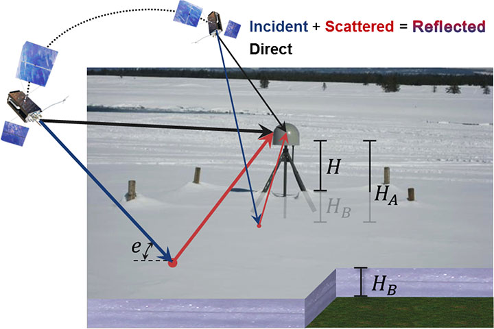
    FIGURE 1. Standard geodetic receiver installation. The antenna is protected by a hemispherical radome. The monument (tripod structure) is ~ 2 meters above the ground. GPS satellites rise and set in ascending and descending sky tracks, multiple times per day. The specular reflection point migrates radially away from the receiver for decreasing satellite elevation angle. The total reflector height is made up of an a priori value and an unknown bias driven by the thickness of the snow layer.
    FIGURE 1. Standard geodetic receiver installation. The antenna is protected by a hemispherical radome. The monument (tripod structure) is ~ 2 meters above the ground. GPS satellites rise and set in ascending and descending sky tracks, multiple times per day. The specular reflection point migrates radially away from the receiver for decreasing satellite elevation angle. The total reflector height is made up of an a priori value and an unknown bias driven by the thickness of the snow layer.

    In this article, we summarize the SNR-based GPS-MR technique as applied to snow sensing using geodetic instruments. This forward/inverse approach for GPS-MR is new in that it capitalizes on known information about the antenna response and the physics of surface scattering to aid in retrieving the unknown snow conditions in the site surroundings. It is a statistically rigorous retrieval algorithm, agreeing to first order with the simpler original methodology, which is retained here for the inversion bootstrapping. The first part of the article describes the retrieval algorithm, while the second part provides validation at a representative site over an extended period of time. 

    Physical Forward Model

    SNR observations are formulated as SNR = Ps/Pn. In the denominator, we have the noise power, Pn, here taken as a constant, based on nominal values for the noise power spectral density and the noise bandwidth. The numerator is composite signal power:

    Eq-1.   (1)

    Its incoherent component is the sum of the respective direct and reflected powers (although direct incoherent power is negligible). In contrast, the coherent composite signal power follows from the complex sum of direct and reflection average voltages (not to be confused with the electromagnetic propagating fields, which neglect the receiving antenna response and also the receiver tracking process):

    Eq-2(2)

    It is expressed in terms of the coherent direct and reflected powers, as well as the interferometric phase,

    Eq-3 , (3)

    which amounts to the reflection excess phase with respect to the direct signal.

    We decompose observations, SNR = tSNR + dSNR, into a trend

    Eq-4  (4)

    over which interference fringes are superimposed:

    Eq-5. (5) 

    From now on, we neglect the incoherent power, which only impacts tSNR, not dSNR, and drop the coherent power superscript, for brevity.

    The direct or line-of-sight power is formulated as

    Eq-6  (6)

    where  Eq-6-a  is the direction-dependent right-hand circularly polarized (RHCP) power component incident on an isotropic antenna; the left-handed circularly polarized (LHCP) component is negligible. The direct antenna gain, Eq-6-b, is obtained evaluating the antenna pattern in the satellite direction and with RHCP polarization.

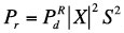
    The reflection power,
    Eq-7, (7)

    is defined starting with the same incident isotropic power, Eq-6-a, as in the direct power. It ends with a coherent power attenuation factor, 

    Eq-8  (8)

    where  θ  is the angle of incidence (with respect to the surface normal), k = 2π/λ, is the wave number, and λ = 24.4 centimeters is the carrier wavelength for the civilian GPS signal on the L2 frequency (L2C). This polarization-independent factor accounts only for small-scale residual height above and below a large-scale trend surface. The former/latter results from high-/low-pass filtering the actual surface heights using the first Fresnel zone as a convolution kernel, roughly speaking. Small-scale roughness is parameterized in terms of an effective surface standard deviation s (in meters); its scattering response is modeled based on the theories of random surfaces, except that the theoretical ensemble average is replaced by a sensing spatial average. Large-scale deterministic undulations could be modeled, but their impact on snow depth is canceled to first-order by removing bare-ground reflector heights.

    At the core of Eq-Pr, we have coupled surface/antenna reflection coefficients,  Eq-X=, producing respectively RHCP and LHCP fields (under the assumption of a RHCP incident field). These terms include antenna response power gain and phase patterns, evaluated in the reflection direction, and separately for each polarization. The surface response is represented by complex-valued Fresnel coefficients for cross- and same-sense circular polarization, respectively. The medium is assumed to be homogeneous (that is, a semi-infinite half-space). Material models provide the complex permittivity, which drives the Fresnel coefficients.
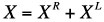
    The interferometric phase reads:
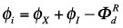
    Eq-9.(9)

    The first term accounts for the surface and antenna properties of the reflection, as above. The last one is the direct phase contribution, which amounts to only the RHCP antenna phase-center variation evaluated in the satellite direction. The majority of the components present in the direct RHCP phase (such as receiver and satellite clock states, the bulk of atmospheric propagation delays, and so on) are also present in the reflection phase, so they cancel out in forming the difference.

    At the core of the interferometric phase, we have the geometric component, φI = i, the product of the wave number and the interferometric propagation delay. Assuming a locally horizontal surface, the latter is simply:
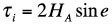
    Eq-10  (10)

    in terms of the satellite elevation angle, e, and an a priori reflector height, HA. Snow depth will be measured in terms of changes in reflector height.

    The physical forward model, based only on a priori information, can then be summarized as:

    Eq-11a  (11)

    where interferometric power and phase are, respectively:
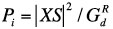
     Eq-12 (12)

    Eq-13. (13)

    In all of these terms the pseudorandom-noise-code modulation impressed on the carrier wave can be safely neglected, given the small interferometric delay and Doppler shift at grazing incidence, stationary surface/receiver conditions, and short antenna installations.

    Parameterization of Unknowns

    There are errors in the nominal values assumed for the physical parameters of the model (permittivity, surface roughness, reflector height, and so on). Ideally we would estimate separate corrections for each one, but unfortunately many are linearly dependent or nearly so. Because of this dependency, we have kept physical parameters fixed to their optimal a priori values, and have estimated a few biases. Each bias is an amalgamation of corrections for different physical effects. In a later stage, we rely on multiple independent bias estimates (such as for successive days) to try and separate the physical sources.

    Each satellite track is inverted independently. A track is defined by partitioning the data by individual satellite and then into ascending and descending portions, splitting the period between the satellite’s rise and set at the near-zenith culmination. Each satellite track has a duration of ~1–2 hours. This configuration normally offers a sufficient range of elevation angles, unless the satellite reaches culmination too low in the sky (less than about 20°), in which case the track is discarded. In seeking a balance between under- and over-fitting, between an insufficient and an excessive number of parameters, we estimate the following vector of unknown parameters:

    Eq-14. (14)

    FIGURE 2 shows the effect of the constant and linear biases on the SNR observations. Reflector height bias, HB , changes the number of oscillations; phase shift, φB , displaces the oscillations along the horizontal axis; reflection power, Eq-14-a   , affects the depth of fades; zeroth-order noise power,   Eq-14-b  , shifts the observations up or down as a whole; and first-order noise power,  Eq-14-c  , tilts the SNR curve. A good parameterization yields observation sensitivity curves as unique as possible for each parameter.
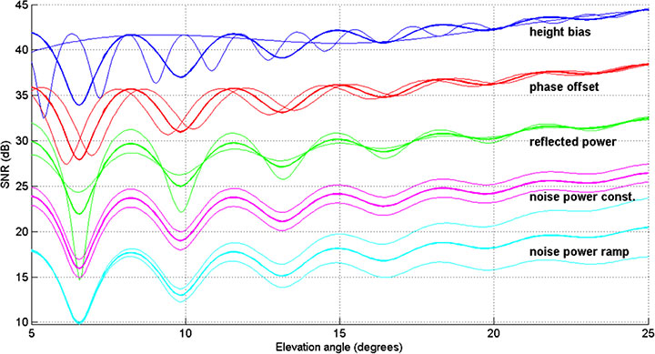
    FIGURE 2. Effect of each parameter on SNR observations; curves are displaced vertically (6 dB) for clarity.
    FIGURE 2. Effect of each parameter on SNR observations; curves are displaced vertically (6 dB) for clarity.

    The forward model, now including the biases, can be summarized as follows:

    Eq-15 (15)

    where the modified interferometric power and phase are given by:
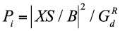
    Eq-16, (16)

    Eq-17. (17)

    The total reflector height, H = HAHB (a priori value minus unknown bias), is to be interpreted as an effective value that best fits measurements, which includes snow and other components.

    Bootstrapping Parameter Priors. Biases and SNR observations are involved non-linearly through the forward model. Therefore, there is the need for a preliminary global optimization, without which the subsequent final local optimization will not necessarily converge to the optimal solution.

    SNR observations would trace out a perfect sinusoid curve in the case of an antenna with isotropic gain and spherical phase pattern, surrounded by a smooth, horizontal, and infinite surface (free of small-scale roughness, large-scale undulations, and edges), made of perfectly electrically conducting material, and illuminated by constant incident power. Thus, in such an idealized case, SNR could be described exactly by constant reflector height, phase shift, amplitude, and mean values.

    As the measurement conditions become more complicated, the SNR data start to deviate from a pure sinusoid. Yet a polynomial/spectral decomposition is often adequate for bootstrapping purposes. 

    Statistical Inverse Model Formulation

    Based on the preliminary values for the unknown parameters vector and other known (or assumed) values, we run the forward model to obtain simulated observations. We form pre-fit residuals comparing the model values to SNR measurements collected at varying satellite elevation angles (separately for each track). Residuals serve to retrieve parameter corrections, such that the sum of squared post-fit residuals is minimized. This non-linear least squares problem is solved iteratively using both a functional model and a stochastic model. The functional modeling includes a Jacobian matrix of partial derivatives, which represents the sensitivity of observations to parameter changes where the partial derivatives are defined element-wise. Instead of deriving analytical expressions, we evaluate them numerically, via finite differencing. The stochastic model specifies the uncertainty and correlation expected in the residuals. Their a priori covariance matrix modifies the objective function being minimized. 

    Directional Dependence

    It is important to know at which elevation angles the parameter estimates are best determined. Here, we focus on the phase parameters instead of reflection power or noise power parameters. 

    We can utilize the estimated reflector height and phase shift to evaluate the full phase bias function over varying elevation angles. Similarly, we can extract the corresponding 2-by-2 portion of the parameters’ a posteriori covariance matrix, containing the uncertainty for reflector height and for phase shift, as well as their correlation, which is then propagated to obtain the full phase uncertainty (see FIGURE 3).
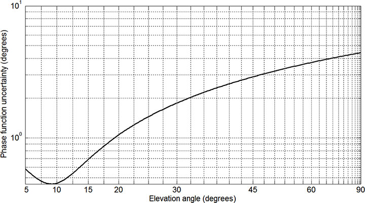
    FIGURE 3. Uncertainty of full phase function, propagated from the uncertainty of reflector height and of phase shift, as well as their correlation.
    FIGURE 3. Uncertainty of full phase function, propagated from the uncertainty of reflector height and of phase shift, as well as their correlation.

    The uncertainty attains a clear minimum versus elevation angle. The least-uncertainty elevation angle pinpoints the observation direction where reflector height and phase shift are best determined (in combined form, not individually). The azimuth and epoch coinciding with the peak elevation angle act as track tags, later used for clustering similar tracks and analyzing their time series of retrievals.

    If we normalize phase uncertainty by its value at the peak elevation angle, then plot such sensing weights (between 0 and 1) versus the radial or horizontal distance to the center of the first Fresnel zone at each elevation angle, we obtain FIGURE 4. It can be interpreted as the reflection footprint, indicating the importance of varying distances, with a longer far tail and a shorter near tail (respectively regions beyond and closer than the peak distance). The implications for in situ data collection are clear: one should sample more intensely near the peak distance (about 15 meters) and less so in the immediate vicinity of the GPS antenna, tapering it off gradually away from the antenna. As a caveat, these conclusions are not necessarily valid for antenna setups other than the one considered here.
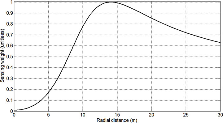
    FIGURE 4. Reflection footprint in terms of a sensing weight (between 0 and 1) defined as the normalized reciprocal of full phase uncertainty, plotted versus the radial or horizontal distance from the receiving antenna to the center of the first Fresnel zone at each elevation angle; valid for an upright 2-meter-tall antenna; the receiving antenna is at zero radial distance.
    FIGURE 4. Reflection footprint in terms of a sensing weight (between 0 and 1) defined as the normalized reciprocal of full phase uncertainty, plotted versus the radial or horizontal distance from the receiving antenna to the center of the first Fresnel zone at each elevation angle; valid for an upright 2-meter-tall antenna; the receiving antenna is at zero radial distance.

    Results

    We now examine the snow-depth retrievals from the GPS multipath retrieval algorithm and assess both the precision and accuracy of the method. Multiple metrics have been developed to assess the quality of the results. The accuracy of the method has been evaluated by comparing with in situ data over a multi-year period. Three field sites were chosen to highlight different limitations in the method, both in terms of terrain and forest cover: grassland, alpine, and forested. We will look at the forested site in some detail.

    Satellite Coverage and Track Clustering. All GPS-MR retrievals reported here are based on the newer GPS L2C signal. Of the approximately 30 GPS satellites in service, 8-10 L2C satellites were available between 2009 and 2012 (8, 9, and 10 satellites at the end of 2009, 2010, and 2011, respectively). Satellite observations were partitioned into ascending and descending portions, yielding approximately twenty unique tracks per day at a site with good sky visibility. GPS orbits are highly repeatable in azimuth, with deviations at the few-degree range over a year, translating into ~50-100-centimeter azimuthal displacement of the reflecting area (corresponding to the first Fresnel zone at 10°-15° elevation angle for a 2-meter high antenna). This repeatability permits clustering daily retrievals by azimuth. It also allows the simplification that estimated snow-free reflector heights are fairly consistent from day to day, facilitating the isolation of the varying snow depth during the snow-covered period.

    For a given track, its revisit time is also repeatable, amounting to practically one sidereal day. The deficit in time relative to a calendar day results in the track time of the day receding ~4 minutes and 6 seconds every day. This slow but steady accumulation eventually makes the time of day return to its starting value after about one year. As all GPS satellites drift approximately at the same rate, the time between successive tracks remains nearly repeatable. Its reciprocal, the sampling rate, has a median equal to approximately one track per hour, with a low value of one track within two hours and a high of one track within 15 minutes; both extremes occur every day, with low-rate idle periods interspersed with high-rate bursts. The time of the day reduced to a fixed day (such as January 1, 2000) could also be used to cluster tracks. Neighboring clusters, which are close in azimuth and/or in reduced time of the day, are expected to be more comparable, as they sample similar conditions and are subject to similar errors.

    Observations. FIGURE 5 shows several representative examples of SNR observations. A typical good fit between measured and modeled values is shown in Figure 5(a), corresponding to the beginning of the snow season. Generally the model/measurement fit is good when the scattering medium is homogeneous; it deteriorates as the medium becomes more heterogeneous, particularly with mixtures of soil, snow, and vegetation. There are genuine physical effects as well as more mundane spurious instrumental issues that degrade the fit but do not necessarily cause a bias in snow-depth estimates. These include secondary reflections, interferometric power effects, direct power effects, and instrument-related issues.
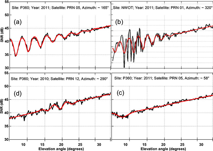
    FIGURE 5. Examples of observations: (a) good fit; (b) presence of secondary reflections; (c) vanishing interference fringes; (d) atypical interference fringes.
    FIGURE 5. Examples of observations: (a) good fit; (b) presence of secondary reflections; (c) vanishing interference fringes; (d) atypical interference fringes.

    Secondary reflections originate from disjoint surface regions. Interference fringes become convoluted with multiple superimposed beats (see Figure 5(b)). As long as there is a unique dominating reflection, the inversion will have no difficulty fitting it, as the extra reflections will remain approximately zero-mean.

    Random deviations of the actual surface with respect to its undulated approximation, called roughness or residual surface height, will affect the interferometric power. SNR measurements will exhibit a diminishing number of significant interference fringes, compared to the measurement noise level (see Figure 5(c)). This facilitates the model fit but the reflector height parameter may become ill-determined: its estimates will be more uncertain. Changes in snow density also affect the fringe amplitude.

    Snow precipitation attenuates the satellite-to-ground radio link, which affects SNR measurements through the direct power term. First, this shifts the SNR measurements up or down (in decibels); second, it tilts the trend tSNR as attenuation is elevation-angle dependent; third, fringes in dSNR will change in amplitude because of the decrease in the coherent component of the direct power.

    Partial obstructions can affect either or both direct and interferometric powers. In this case, SNR measurements, albeit corrupted, are still recorded. This situation is in contrast to complete blockages as caused by topography. The deposition of snow and the formation of a winter rime on the antenna are a particularly insidious type of obstruction, as their presence in the near-field of the antenna element can easily distort the gain pattern in a significant manner. In the far-field, trees are another important nuisance, so much so that their absence is held as a strong requirement for the proper functioning of multipath reflectometry.

    Satellite-specific direct power offsets and also long-term power drifts are to be expected as spacecraft age and modernized designs are launched. In addition, noise power depends on the state of conservation of receiver cables and on their physical temperature. Less subtle incidents are sudden ~3-dB SNR steps, hypothesized to originate in the receiver switching between the L2C data and pilot subcodes, CM and CL.

    Quality Control. Anomalous conditions may result in measurement spikes, jumps, and short-lived rapidly-varying fluctuations. For snow-depth-sensing purposes, it is necessary and sufficient to either neutralize such measurement outliers through a statistically robust fit or detect unreliable fits and discard the problematic ones that could not otherwise be salvaged.

    The key to quality control (QC) is in grouping results into statistically homogeneous units, having measurements collected under comparable conditions. In our case, azimuth-clustered tracks are the natural starting unit. Secondarily, we must account for genuine temporal variations in the tendency of results, from beginning to peak to the end of the snow season. The detection of anomalous results further requires an estimate of the statistical dispersion to be expected. Considering that the sample is contaminated with outliers, robust estimators (running median instead of the running mean, and median absolute deviation over the standard deviation) are called for, if the first- and second-order statistical moments are to be representative. Given estimates of the non-stationary tendency and dispersion, a tolerance interval can then be constructed such that it bounds, say, a 99% proportion of the valid results with 95% confidence level. We also desire QC to be judicious, or else too many valid estimates will be lost. Notice that in the present intra-cluster QC, we compare an individual estimate to the expected performance of the track cluster to which it belongs; later, we complement QC with an inter-cluster comparison of each cluster’s own expected performance.

    Based on our practical experience, no single statistic detects all the outliers. We use four particular statistics that we have found to be useful: 1) degrees of freedom, essentially the number of observations per track (modulo a constant number of parameters); 2) using the scaled root-mean-square error (RMSE) to test for goodness-of-fit, that is, how well measurements can be explained adjusting the unknown values for the parameters postulated in the model; 3) reflector height uncertainty; and 4) peak elevation angle, which behaves much like a random variable, as it is determined by a multitude of factors. 

    Combinations. We combine multiple clusters to average out random noise. Noise mitigation aims at not only coping with measurement errors but also compensating for model deficiencies, to the extent that they are not in common across different clusters. Before we combine different clusters, we have to address their long-term differences. The initial situation is that snow surface heights will be greater downhill and smaller uphill; we take this into account on a cluster-by-cluster basis by subtracting ground heights from their respective snow surface heights, resulting in snow thickness values, which is a completely physically unambiguous quantity. Snow thickness is more comparable than snow heights across varying-azimuth track clusters. Yet snow tends to fill in ground depressions, so thickness exhibits variability caused by the underlying ground surface, even when the overlying snow surface is relatively uniform. Further cluster homogeneity can be achieved by accounting for the temporally permanent though spatially non-uniform component of snow thickness. 

    The averaging of snow depths collected for different track clusters employs the inversion uncertainties to obtain a preliminary running weighted median, calculated for, say, daily postings, with overlapping windows or not. The preliminary post-fit residuals then go through their own averaging, necessarily employing a wider averaging window (say, monthly), which produces scaling factors for the original uncertainties. The running weighted median is then repeated, producing final averages. The variance factors reflect the fact that some clusters are better than others.

    Thus, the final GPS estimates of snow depth follow from an averaging of all available tracks, whose individual snow depth values were previously estimated independently. A new average is produced twice daily utilizing the surrounding 1–2 days of data (depending on the data density), that is, 12-hour posting spacing and 24-hour moving window width. The averaging interval must be an integer number of days, so as to minimize the possibility of snow-depth artifacts caused by variations in the observation geometry, which repeats daily.

    Site-Specific Results

    We explored GPS-MR snow-depth retrieval at three stations over a long period (up to three years). Throughout, we assessed the performance of the GPS estimates against independent nearly co-located in situ measurements. We also compared the GPS estimates to the nearest SNOTEL station. SNOTEL (from snowpack telemetry) is an automated system for collecting snowpack and related data in the western U.S. operated by the U.S. Department of Agriculture. Although not co-located with GPS, SNOTEL data are important because they provide accurate information on the timing of snowfall events.

    The three sites we used were 1) a site in the T.W. Daniel Experimental Forest within the Wasatch Cache National Forest in the Bear River Range of northeastern Utah, with an elevation of 2,600 meters; 2) one of the stations of the EarthScope Plate Boundary Observatory, a grassland site located near Island Park, Idaho; and 3) an alpine site in the Niwot Ridge Long-term Ecological Research Site near Boulder, Colorado. While we have fully documented the results from each site, due to space limitations we will only discuss the results from the forested site (known as RN86) in this article. This is a more challenging site than the other two, due to the presence of nearby trees. Furthermore, it was subject to denser in situ sampling of 20-150 measurements spatially replicated around the GPS antenna, and repeated approximately every other week for about one year.

    We show results for the 2012 water-year, the period starting October 1 through September 30 of the following year. Where GPS site RN86 was installed, topographical slopes range from 2.5° to 6.5° (at the 2-meter spatial scale), with average of ~5° within a 50-meter radius around the GPS antenna. RN86 was specifically built to study the impact of trees on GPS snow depth retrievals (see FIGURE 6). Ground crews manually collected in situ measurements around the GPS antenna approximately every other week starting in November 2011. Measurements were made every 1–2 meters from the antenna up to a distance of 25-30 meters. In the second half of the year, the sampling protocol was changed to azimuths of 0° (N), 45° (NE), 135° (SE), 180° (S), 225° (SW), and 315° (NW). With these data it is possible to obtain in situ average estimates, with their own uncertainties (based on the number of measurements), which allows a more meaningful comparison.
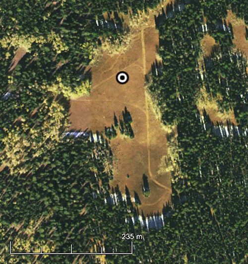
    FIGURE 6. Aerial view of the forested site (RN86) around the GPS antenna (marked with a circle).
    FIGURE 6. Aerial view of the forested site (RN86) around the GPS antenna (marked with a circle).

    There is reduced visibility at the current site, compared to other sites. Track clusters are concentrated due south, with only two clusters located within ±90° of north. Therefore, the GPS average snow depth is not necessarily representative of the azimuthally symmetric component of the snow depth. In the presence of an azimuthal asymmetry in the snow distribution around the antenna, the GPS average would be expected to be biased towards the environmental conditions prevalent in the southern quadrant. To rule out the possibility of an azimuthal artifact in the comparisons, we have utilized only the in situ data collected along the SE/S/SW quadrant.

    The comparison shows generally excellent agreement between GPS and in situ data (see FIGURE 7). The first four and the last one in situ data points were collected with coarser spacing and/or smaller azimuthal coverage, which may be partially responsible for different performance in the first and second halves of the snow season. The correlation between GPS and in situ snow depth at RN86 amounts to 0.990, indicating a very strong linear relationship. Carrying out a regression between in situ and GPS values, the RMS of snow-depth residuals improves from 9.6 to 3.4 centimeters. The regression intercept and slope (with corresponding 95% uncertainties) amount to 15.4 ± 9.11 centimeters and 0.858 ± 0.09 meters per meter, respectively. According to these statistics, the null hypotheses of zero intercept and unity slope are rejected at the 95% confidence level. This implies that at this location GPS snow-depth estimates exhibit both additive and multiplicative biases. The latter is proportional to snow depth itself, meaning that, compared to an ideal one-to-one relationship, GPS is found to under-estimate in situ snow depth at this site by 14 ± 9%, although the uncertainty is somewhat large.
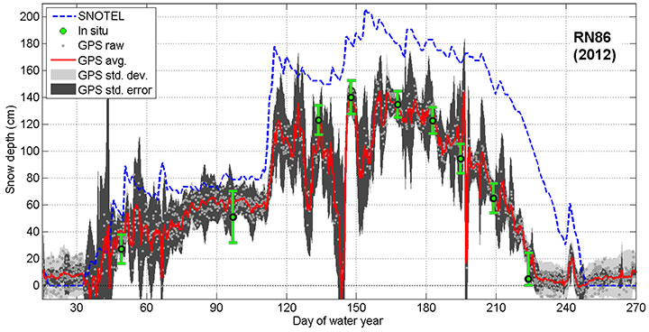
    FIGURE 7. Snow-depth measurement at the forested site (RN86) for the water-year 2012
    FIGURE 7. Snow-depth measurement at the forested site (RN86) for the water-year 2012

    The SNOTEL sensors are exceptionally close to the GPS antenna at this site, about 350 meters horizontally distant with negligible vertical separation. Yet the former is located within trees, while the latter is located at the periphery of the forest and senses the reflections scattered from an open field. Therefore, only the timing of snowfall events agrees well, not the amount of snow. Although forest density is generally negatively correlated with snow depth, exceptions are not uncommon, especially in localized clearings exposed to intense solar radiation, where shading of the snow by the trees reduces ablation.

    Conclusions

    In this article, we have discussed a physically based forward model and a statistical inverse model for estimating snow depth based on GPS multipath observed in SNR measurements. We assessed model performance against independent in situ measurements and found they validated the GPS estimates to within the limitations of both GPS and in situ measurement errors after the characterization of systematic errors. The assessment yielded a correlation of 0.98 and an RMS error of 6–8 centimeters for observed snow depths of up to 2.5 meters at three sites, with the GPS underestimating in situ snow depth by ~5–15%. This latter finding highlights the necessity to assess effects currently neglected or requiring more precise modeling.

    Acknowledgments

    The research reported in this article was supported by grants from the U.S. National Science Foundation, NASA, and the University of Colorado. Nievinski has been supported by a Capes/Fulbright Graduate Student Fellowship and a NASA Earth System Science Research Fellowship. The article is based, in part, on two papers published in the IEEE Transactions on Geoscience and Remote Sensing: “Inverse Modeling of GPS Multipath for Snow Depth Estimation – Part I: Formulation and Simulations” and “Inverse Modeling of GPS Multipath for Snow Depth Estimation – Part II: Application and Validation.”

    Manufacturers

    For the forested site (RN86), a Trimble NetR9 receiver was used with a Trimble TRM57971.00 (Zephyr Geodetic II) antenna with no external radome.


    FELIPE G. NIEVINSKI is a faculty member at the Federal University of Santa Catarina, Florianópolis, Brazil. He has also been a post-doctoral researcher at São Paulo State University, Presidente Prudente, Brazil. He earned a B.E. in geomatics from the Federal University of Rio Grande do Sul, Porto Alegre, Brazil, in 2005; an M.Sc.E. in geodesy from the University of New Brunswick, Fredericton, Canada, in 2009; and a Ph.D. in aerospace engineering sciences from the University of Colorado, Boulder, in 2013. His Ph.D. dissertation was awarded The Institute of Navigation Bradford W. Parkinson Award in 2013.

    KRISTINE M. LARSON received a B.A. degree in engineering sciences from Harvard University and a Ph.D. degree in geophysics from the Scripps Institution of Oceanography, University of California at San Diego. She was a member of the technical staff at the Jet Propulsion Lab from 1988 to 1990. Since 1990, she has been a professor in the Department of Aerospace Engineering Sciences, University of Colorado, Boulder.


    FURTHER READING

    • Authors’ Journal Papers

    “Inverse Modeling of GPS Multipath for Snow Depth Estimation—Part I: Formulation and Simulations” by F.G. Nievinski and K.M. Larson in IEEE Transactions on Geoscience and Remote Sensing, Vol. 52, No. 10, 2014, pp. 6555–6563, doi: 10.1109/TGRS.2013.2297681.

    “Inverse Modeling of GPS Multipath for Snow Depth Estimation—Part II: Application and Validation” by F.G. Nievinski and K.M. Larson in IEEE Transactions on Geoscience and Remote Sensing, Vol. 52, No. 10, 2014, pp. 6564–6573, doi: 10.1109/TGRS.2013.2297688.

    • More on the Use of GPS for Snow Depth Assessment

    “Snow Depth, Density, and SWE Estimates Derived from GPS Reflection Data: Validation in the Western U.S.” by J.L. McCreight, E.E. Small, and K.M. Larson in Water Resources Research, published first on line, August 25, 2014, doi: 10.1002/2014WR015561.

    Environmental Sensing: A Revolution in GNSS Applications” by K.M. Larson, E.E. Small, J.J. Braun, and V.U. Zavorotny in Inside GNSS, Vol. 9, No. 4, July/August 2014, pp. 36–46.

    Snow Depth Sensing Using the GPS L2C Signal with a Dipole Antenna” by Q. Chen, D. Won, and D.M. Akos in EURASIP Journal on Advances in Signal Processing, Special Issue on GNSS Remote Sensing, Vol. 2014, Article No. 106, 2014, doi: 10.1186/1687-6180-2014-106.

    “GPS Snow Sensing: Results from the EarthScope Plate Boundary Observatory” by K.M. Larson and F.G. Nievinski in GPS Solutions, Vol. 17, No. 1, 2013, pp. 41–52, doi: 10.1007/s10291-012-0259-7.

    • GPS Multipath Modeling and Simulation

    “Forward Modeling of GPS Multipath for Near-Surface Reflectometry and Positioning Applications” by F.G. Nievinski and K.M. Larson in GPS Solutions, Vol. 18, No. 2, 2014, pp. 309–322, doi: 10.1007/s10291-013-0331-y.

    “An Open Source GPS Multipath Simulator in Matlab/Octave” by F.G. Nievinski and K.M. Larson in GPS Solutions, Vol. 18, No. 3, 2014, pp. 473–481, doi: 10.1007/s10291-014-0370-z.

    Multipath Minimization Method: Mitigation Through Adaptive Filtering for Machine Automation Applications” by L. Serrano, D. Kim, and R.B. Langley in GPS World, Vol. 22, No. 7, July 2011, pp. 42–48.

    It’s Not All Bad: Understanding and Using GNSS Multipath” by A. Bilich and K.M. Larson in GPS World, Vol. 20, No. 10, October 2009, pp. 31–39.

    GPS Signal Multipath: A Software Simulator” by S.H. Byun, G.A. Hajj, and L.W. Young in GPS World, Vol. 13, No. 7, July 2002, pp. 40–49.
  • 25th Anniversary GNSS Timeline

    GPS_World_25_Year_Timeline_Page1

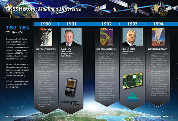
    GPS World’s 25th Anniversary GNSS History Timeline, from the September 2014 Special Supplement “GNSS Industry: Past, Present, and Future.” Download the PDF.

  • Multi-Constellation. Dual-Frequency. Single-Chip.

    Multi-Constellation. Dual-Frequency. Single-Chip.

    NAPA-OpeningFigure


    Fully Integrated NAPA Receiver Brings Mass-Market Potential

    This integrated circuit supports simultaneous reception and processing of the GPS L1/L5, Galileo E1/E5a, and GLONASS G1 signals with 40 tracking channels. The dual-band analog RF front-end is integrated on the same mixed-signal chip as the baseband hardware, including an embedded processor to close the tracking loops: overall, a compact, low-power, and low-cost solution.

    By Fabio Garzia, Stefan Köhler, Santiago Urquijo, Philipp Neumaier,Jörn Driesen, Sybille Haas, Thomas Leineweber, Tao Zhang, Sascha Krause, Frank Henkel,Alexander Rügamer, Matthias Overbeck, and Günther Rohmer

    Multi-constellation multi-band global navigation satellite system (GNSS) receivers can efficiently exploit the advantages derived from the modernization of existing GNSS constellations, such as GPS and GLONASS, as well as from the launch of new ones like Galileo and BeiDou. Utilizing multiple systems can significantly improve the availability of a navigation solution in urban canyons and heavily shadowed areas. Increased satellite availability also guarantees higher measurement redundancy and improved reliability. Moreover, the excellent inherent noise and multipath mitigation capabilities of the new and modernized wideband signals in the L5/E5a band, combined with the ionosphere error mitigation given by frequency diversity, significantly improves the accuracy in both measurement and position domains.

    Still, most commercial fully-integrated single-chip mass market GNSS receivers use only a single-frequency band for their positioning, velocity, time (PVT) solution: either GPS L1 C/A or Galileo E1 and GLONASS G1. For example, the Teseo chips are single-chip solutions that support multiple constellations but only on one frequency band. This approach reduces  design costs and enables the lowest consumption of power, but neglects the advantages of wideband signal processing  – which offers increased robustness thanks to  two simultaneous frequency band receptions and the capability of mitigating the ionosphere error.

    Another approach for realizing multi-constellation multi-frequency solutions is to combine different chips for the analog front-end and the digital baseband. One fully integrated single-chip analog multi-band front-end for the simultaneous reception of GPS L1/L5, Galileo E1/E5, and GLONASS has been presented. However, this chip included only the front-end and requires an additional, separate digital-baseband solution.

    The purpose of the NAPA project (NAvigation chip for Pedestrian navigation and higher precision Applications) is to close this gap by providing a fully integrated, compact, low-power, and low-cost solution in which the analog and digital parts of the GNSS receiver are integrated together on the same chip. The NAPA receiver offers all the advantages of multi-constellation reception with additional dual-frequency support.

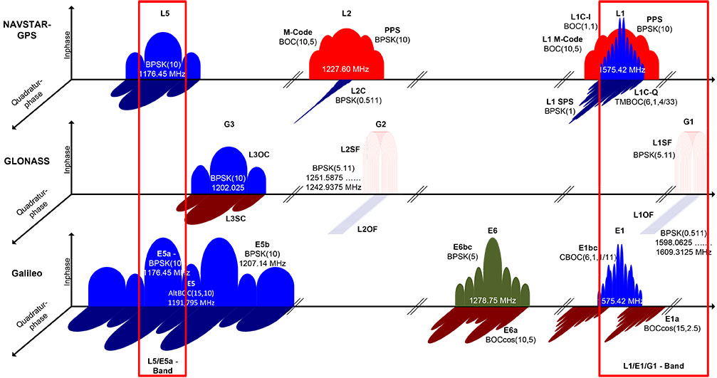
    The NAPA chip features a monolithic, single mixed-signal chip implementation of a multi-system, multi-band analog front-end and the related digital baseband core, including an embedded processor. The NAPA chip can be used as a stand-alone GNSS sensor, because no additional components are required to obtain a PVT solution. The ASIC was implemented in a low-power technology and adopts some ad-hoc low-power architectural features. In regard to costs, an ASIC solution is more convenient than FPGA,  provided the non-recurring engineering costs (NRE) are amortized by the amount of chips manufactured and sold. The NAPA chip supports multi-system (GPS, Galileo, and GLONASS) and multi-band (GPS/Galileo L1/E1, L5/E5a, GLONASS G1) processing. Figure 1 shows the frequency band being selected for receiving and processing in the NAPA chip. With two fully deployed GNSS — GPS and GLONASS — NAPA chips can already be used in many commercial applications. Thanks to the spectral overlay of the GPS L1/L5 and Galileo E1/E5a signals, the chip is also ready for Galileo. The frequency selection features both the narrow-band legacy signals L1/G1, which can be used for fast acquisition. For highest tracking accuracy, the wideband GPS L5 and Galileo E5a BPSK(10) modulated signals can be utilized.

    Figure 1. GNSS signals received and processed by the NAPA chip.
    Figure 1. GNSS signals received and processed by the NAPA chip.

    The higher accuracy is  obtained primarily by the attenuation of the ionospheric error. The ionosphere is a dispersing media that can introduce a bias error between 1 and 20 m. Forming a linear combination of two independent frequency-band measurements, the ionospheric bias can be measured and almost completely removed. In addition, Precise Point Positioning and Wide/Narrow-laning combinations are possible, thanks to the second received frequency band. The first allows for the combination of precise satellite positions and clocks with multi-frequency measurements, providing cm/dm solutions. The second adopts fast ambiguity solutions for carrier-phase positioning and cycle-slip detection.

    In this article, we present the NAPA chip in detail. We describe the architecture of the analog front-end and its digital counterpart and the innovative features of each. Then we provide details about chip implementation, manufacturing, and test setup. Finally, we present the first verification results and draw conclusions.

    Architecture Overview

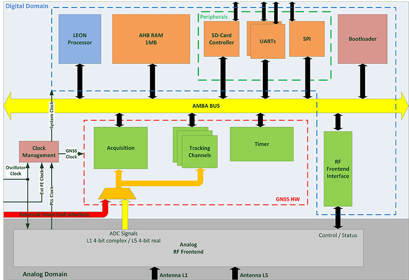
    The NAPA chip architecture, depicted in Figure 2,  is composed of two separate blocks integrated on the same silicon die: the analog core provides the functionality of a two-frequency radio-frequency (RF) front-end, whereas the digital part implements the main GNSS processing tasks, including the correlator channels and an embedded processor, and takes care of the RF front-end control. The interface between the two blocks is completely digital and provides synchronizers to ensure a valid clock domain crossing (CDC).

    Figure 2. Overall NAPA architecture with emphasis on the digital core blocks.
    Figure 2. Overall NAPA architecture with emphasis on the digital core blocks.

    Analog Front-End. The analog RF front-end supports the simultaneous reception of GPS L5 / Galileo E5a and GPS L1 / Galileo E1 / GLONASS G1 signals as well as modes where only one reception path is activated.

    Both passive and active GNSS antennas are supported, thanks to integrated low noise amplifiers (LNA). There are two separate signal reception paths for the two frequency bands. The L1/E1/G1 path is characterized by a quasi-zero-IF conversion that mixes the middle frequency between L1/E1 and G1 to zero frequency. The L1/E1 reception bandwidth is up to 14 MHz so as to incorporate the MBOC modulations of Galileo E1 and future GPS L1C signals. A programmable automatic gain control (AGC) controls the complex analog baseband signals before they are digitized with a 4-bit dual-channel analog digital converter (ADC).

    The second reception path receives an L5/E5a signal with up to 20 MHz bandwidth for the BPSK(10) modulated signals. This path uses a low-IF architecture. The signal is down-converted to an intermediate frequency (IF) of 15.345 MHz. The image frequency is suppressed by a polyphase filter. The real-valued analog signal is controlled by an AGC and converted to the digital domain using a single 4-bit ADC. A common phase locked loop (PLL) is used with specific L1/E1/G1 and L5/E5a dividers to generate the mixers’ local oscillator (LO) frequencies. The PLL loop filter is integrated on-chip to minimize external elements. Moreover, automatic filter and voltage-controlled oscillator (VCO) calibrations are included to mitigate process tolerances. The PLL can handle input clock frequencies between 10 and 80 MHz with a recommended clock frequency of 36.115 MHz.

    An SPI core was implemented on the front-end part to facilitate control of the different front-end features. This means it is possible to tune the PLL, to switch off a complete front-end path if the second frequency band is not used and to activate different on-chip calibration procedures.

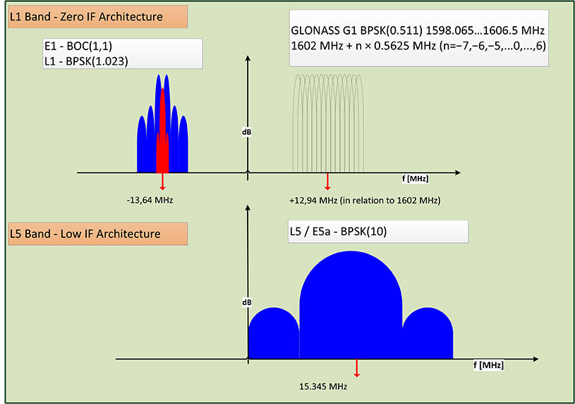
    The frequency plan of the front-end is depicted in Figure 3. Due to the quasi zero-IF architecture, the complex L1/E1 baseband signal is located on an IF of -13.64 MHz and the GLONASS G1 frequency division multiple access (FDMA) signals on an IF of +12.94 MHz, with respect to the GLONASS G1 center frequency of 1602 MHz. The real-valued L5/E5a signals are provided by the second ADC and located on an IF of 15.345 MHz.

    Figure 3. RF front-end frequency plan.
    Figure 3. RF front-end frequency plan.

    The ADC samples are generated with a frequency of 74.4871875 MHz for both the single channel L5, as well as for the dual-channel L1/E1/G1 ADCs. The ADC clock is also directly connected to the baseband digital core and is used as the main clock for the GNSS hardware modules. The embedded processor in the digital core receives a second clock, which is twice as fast as the GNSS hardware one.

    Digital Baseband SoC. The baseband is characterized by a system-on-chip (SoC) architecture based on a SPARC-compatible 32-bit LEON2 microprocessor running at approximately 150 MHz. The GNSS functionality, including acquisition and tracking, are implemented using dedicated hardware modules.

    The processor’s primary functions are to correctly configure the RF front-end and control the different parts of the receiver. In particular, it triggers acquisition, initializes, and starts the tracking channels with the signals detected during acquisition and takes care of closing the frequency/phase/delay locked loops (FLL/PLL/DLL) used for signal tracking. The tracking loops have strict real-time constraints; communication between the channels and the processor features a high-speed infrastructure.

    Structurally, the processor is connected to a hierarchical on-chip Advanced Microcontroller Bus Architecture (AMBA) composed of a high-performance bus (AHB) and a peripheral bus (APB). The AHB provides a direct connection between the processor, the real-time GNSS modules, and the system memory, a monolithic 1 MByte block that hosts the main program at run-time. Different programs can be loaded if needed by using the external SD-card interface.

    In addition to the processor, there are four additional AHB masters: the bootloader, the SD-card controller, the real-time GNSS modules, and the on-chip processor debugger. The bootloader is in charge of the bus control at system start-up. The SD-card controller has integrated direct-memory access (DMA) capabilities to move data between the SD card and the system memory. The real-time GNSS modules can write the tracking results directly to the system memory. Finally, the integrated processor debugger allows real-time debugging and is used mainly in the verification phase. The APB provides a connection to generic peripherals, and control and status interface of the GNSS modules without real-time constraints, as well as the control and status interface of the RF front-end. Since the GNSS modules operate in a separate clock domain that runs at half the frequency of the processor domain, some synchronization logic is necessary to ensure correct CDC.

    The adoption of an SoC architecture provides  higher flexibility than conventional static hardware solutions. In addition to typical GNSS applications, the user can also implement some signal monitoring and processing algorithms in software. The eCos-embedded operating system is provided to ease software development.

    Generic Peripherals. The digital core is equipped with several peripherals that enable the communication with the outside world. The two separate universal asynchronous receiver/transmitter (UART) interfaces can run at 115.2 kbps. A dedicated serial peripheral interface (SPI) master is also provided with a maximum of 10-MHz clock frequency. For example, these interfaces can be used to provide NMEA data to some external display device or raw data (pseudoranges, code phases) in order to calculate a PVT solution. It is also possible to directly access the measurements generated from the correlator hardware and to control the tracking NCOs, which means users can choose their own algorithms for the loop closure. A possible application is the realization of vector-delay tracking using the NAPA ASIC and an external processor.

    The SD-card interface facilitates the loading and storage of large amounts of data, for example, memory codes and almanacs. The possibility of making signal snapshots periodically and saving them to an SD card for later analysis has also been foreseen. This could be useful in special applications in which the receiver hardware is not accessible to the user all of the time.

    In addition, 10 general-purpose I/O pins (GPIO) are provided. They can be controlled via software and can provide a very basic interface (for example, to connect to external LEDs or switches).

    Acquisition Module. The acquisition module adopts a parallel code phase search in the Fourier domain by using a 16-k Samples Fast Fourier Transform (FFT) core. The adopted algorithm is known as parallel code-phase search.

    The L1/E1/G1 signals coming from the front-end are first filtered and then sent to the acquisition module to allow a fast detection of the satellites in the L1/E1/G1 bands with their respective code delays and Doppler frequencies. The acquisition of GLONASS G1 FDMA signals is possible thanks to a software-configurable hardware mixer that can be set with the different G1 carrier frequencies. No direct hardware acquisition is supported for the L5/E5a band signals. The tracking of L5/E5a band signals is possible by performing a hand-over from L1/E1 band or a Tong search using the tracking channels.

    The acquisition process is performed iteratively over all the possible satellites and over a set of Doppler values. These values are obtained by dividing the complete range of possible Doppler variations into bins. The smaller these bins are, the more accurate the acquisition result, but the more time is required to complete the entire process.

    The acquisition has an additional layer of configurability because of the adoption of coherent and incoherent accumulations. These accumulations are supported in hardware but are completely software-controlled. This provides another possibility for achieving  higher accuracy, but at the cost of a larger execution time due to an increase in the amount of accumulations.

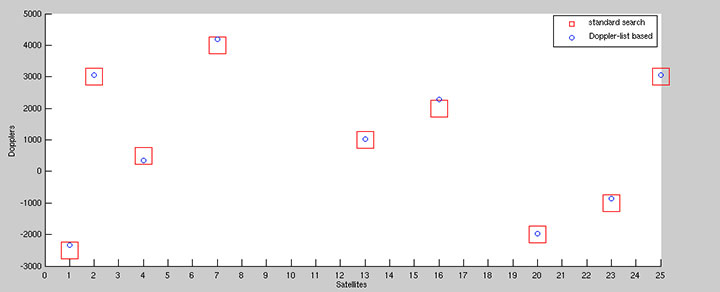
    To speed up acquisition, we introduced a dedicated logic based on a novel patented algorithm. With this algorithm, we are able to detect the Doppler of the L1/E1 satellites present in the signal with an accuracy of 2 Hz. By performing this Doppler search step before the actual acquisition, we are able to generate a list with Doppler values that can be used instead of the bins. This gives more accurate results thanks to the algorithm’s inherent accuracy (see Figure 4) and allows a reduction in the acquisition time since the amount of Doppler values are usually smaller than the bins. Another advantage of this algorithm is the possibility to detect the transition to an indoor context (such as where there is a lack of satellite signals) by simply  looking at the Doppler list, without performing any acquisition.

    Figure 4. Comparison between standard and Doppler-list based acquisition of an L1 signal.
    Figure 4. Comparison between standard and Doppler-list based acquisition of an L1 signal.

    A single iteration step for the acquisition of a GPS L1 signal requires no more than 1 ms for each accumulated epoch. To achieve a good compromise between accuracy and speed, we typically use four epochs of incoherent accumulation, which means approximately 4 ms execution time. For Galileo L1 with four incoherent accumulations, an iteration step takes approximately 16 ms. This time has to be multiplied by the number of satellites and bins to estimate the execution time of the complete process.

    Integrated Acquisition Memories. The acquisition module is characterized by dedicated memory blocks used for the fast FFT processing. It also provides the possibility to use these on-chip memories to store a snapshot of the incoming signals. In particular, we can store up to 81,920 samples of raw data for the complex L1 and real L5 IF signals for further analysis or processing, even off-chip. This enables sophisticated spoofing detection methods, for example, as well as interferer detection and characterization methods. Spoofing detection can be implemented by monitoring the 2D-acquisition search space. Interferer detection and characterization can employ short-time Fourier transforms (STFT) on the snapshot.

    Using the chip as a simple snapshot receiver without having to use the on-chip dedicated GNSS hardware is also a possibilty. For this purpose, the integrated peripherals like UART and SPI ports are provided as interfaces.

    Tracking Module. The 40 versatile tracking channels can be mapped to any combination of GPS, Galileo, and GLONASS signals on the two reception bands. One possible combination would be to track 10 GPS and 10 Galileo satellites simultaneously on both L1/E1 and L5/E5a bands. Alternatively, the user can include GLONASS signals by using fewer GPS / Galileo combinations. The assignment of these tracking channels to the actual GNSS signals can be changed at run-time in order to adapt to different reception situations or to assist the selected signal processing methods.

    Each channel is characterized by a five-tap correlator. For the BPSK modulated signals without side peaks, such as GPS L1/L5, Galileo E5a, and GLONASS G1, we use only three values (early, late, and prompt). For Galileo E1 BOC(1,1) signals, five values are foreseen (very early and very late in addition to the previous), so that false peak lock conditions can be detected and a bump-jumping algorithm can be applied. The switch between these modes can be done at run-time and determines the amount of correlation values to be exchanged between correlators and processor.

    Low-Power Features. The GNSS modules operate in their own clock domain. This clock domain is divided in clock-gated regions. There is a common region for the bus interfaces, one region for the acquisition, and one for each tracking channel. This allows a fine-grain shut-down of the GNSS modules that are not currently in use. For example, the acquisition can be deactivated when there are enough signals in tracking or the unused tracking channels can be disabled. This allows a reduced power consumption for the idle modules. This activation/deactivation procedure is controlled through a set of registers connected to the APB and is performed via software.

    External Front-End Interface. To allow for more flexibility, we provided an additional RF front-end interface. The interface is also depicted in Figure 3. This interface features one 2-bit complex and an additional 2-bit real input, as well as a clock input. The user can decide to directly connect the digital baseband core to an external RF front-end with compatible sampling rate parameters, and exclude the on-chip RF front-end. This makes it possible to use the NAPA chip for validating other RF front-end devices, or it can be adapted to special customer needs.

    Boot-Up Sequence. The SoC includes a hard-coded bootloader that is in charge of the bus control at start-up. In this phase, the processor is switched off. The bootloader loads a 24-kByte program from the SD-card to the system memory and starts the processor. In this phase, the processor runs with the external oscillator clock. Having performed the RF front-end initialization, the processor can switch to the front-end PLL generated processor clock that runs at approximately 150 MHz. This switch is completely transparent to the processor. Then the actual main GNSS receiver program is loaded into the system memory and executed.

    The NAPA Chip

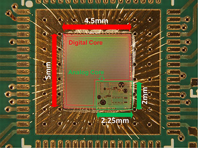
    The NAPA chip has been manufactured in a low-power 1.2 V 65 nm TSMC technology. The 4.5 mm x 5.0 mm chip die was mounted in a QFN68 package; first test samples are available. The core requires a 1.2 V power supply, the pads 1.8 V. Figure 5 shows a picture of the die and its interconnections. The two parts, the analog core and the digital baseband, are clearly distinguishable. The chip is currently in the verification phase.

    Figure 5. NAPA chip.
    Figure 5. NAPA chip.

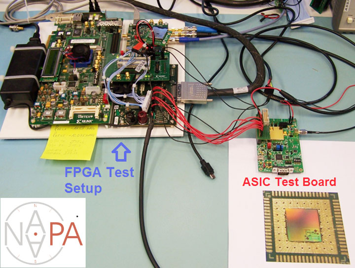
    Within the project, the development and testing of the NAPA design was carried out on basically two platforms. During the hardware development phase, the baseband core has been prototyped on a FPGA device and tested using a special file-player setup, as explained in the following section. Having taped out the chip and received the first samples from the foundry, a test board has been developed in order to verify NAPA chip functionality.

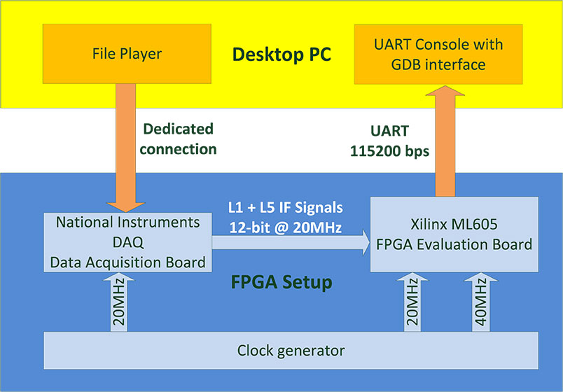
    FPGA Test Setup. In the development phase, the NAPA baseband core has been implemented on a Xilinx Virtex6 FPGA device. A Xilinx ML605 development board has been used for the test setup. The main limitation of the testing in this phase was the lack of an analog RF front-end prototype. In order to make  early testing of GNSS functionality possible, we adopted a file player developed by Fraunhofer IIS in a previous project. This file player uses a desktop PC to reproduce a digital signal data-stream stored in a binary file on the PC. The stream is sent through a dedicated interface to a commercial digital acquisition board. This board receives a clock synchronized with the baseband core’s clock in the FPGA and delivers the signals directly to the FPGA pins. The complete setup is depicted in Figure 6. The setup in use can be seen on the left part of the opening figure.

    Figure 6. FPGA test setup.
    Figure 6. FPGA test setup.

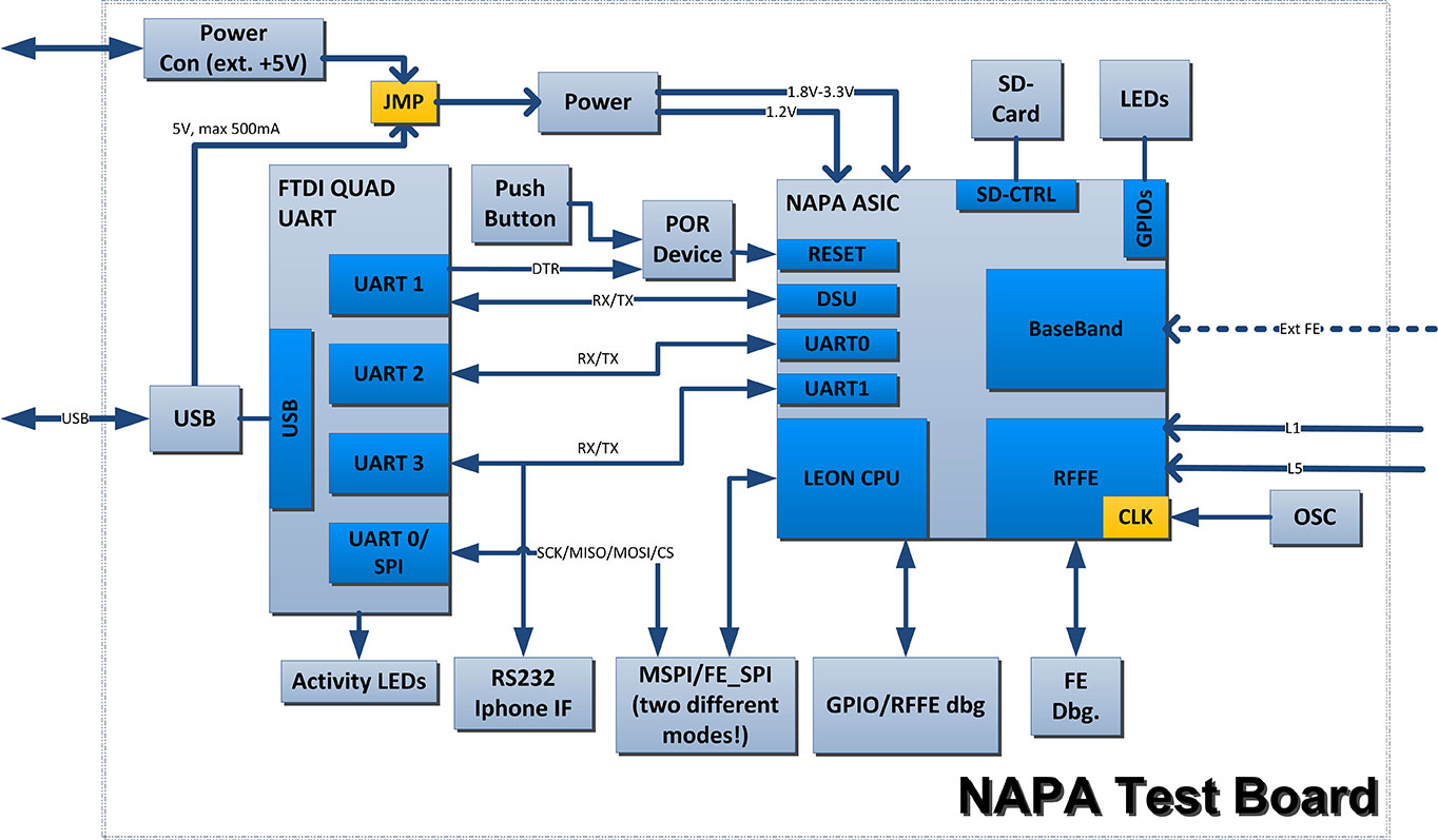
    Test Board. In the verification phase, which is currently ongoing, the first unpackaged test chip dies have been glued directly to the test PCB and bonded on board without any housing. After receiving the packaged chips, the QFN68 could be regularly soldered on the PCB. A block diagram of the board is depicted in Figure 7. The board hosts the typical switch buttons and LEDs for quick control and status detection as well as some specific interfaces. The clock can be provided through a dedicated SMA clock connector as well as a discrete oscillator. Two sub-miniature push-on (SMP) connectors are also provided for separate the L1 and L5 antenna inputs. The two UART ports, the debugger UART, and the SPI master port are connected using a FTDI chip. This chip allows the simultaneous connection of these ports to a desktop PC’s USB port. A parallel connector is provided to interface external front-end ADC signals and clock. The GPIOs are accessible through the same connector. A dedicated socket is added for a mini-SD card.

    Figure 7. Block diagram of NAPA test board.
    Figure 7. Block diagram of NAPA test board.

    Preliminary Results

    The chip on the test board was first tested  using the same file player of the FPGA setup. This way, we could evaluate the correct functionality of the digital baseband core without the need to activate and configure the on-chip front-end. After the successful tests, we focused on the on-chip front-end configuration, and we used the antenna connectors to provide valid GNSS signals. We tested the chip using three different configurations: a GNSS signal simulator, a static roof antenna, and a small active patch antenna.

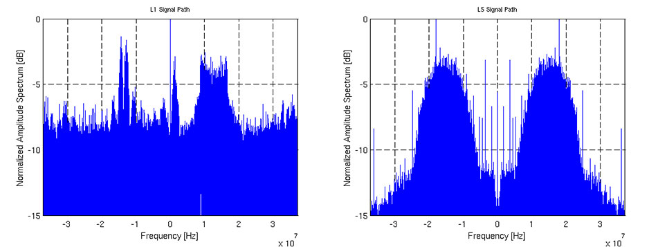
    In the three configurations, we successfully acquired GPS L1 and Galileo E1 signals. We were also able to perform tracking on GPS L1 and L5I, as well as Galileo E1b and E5aI. Figure 8 shows the spectrum of a snapshot of L1 and L5 paths made using the on-chip dedicated snapshot hardware and sent through the UART port with a dedicated binary protocol for offline processing. For this special test, we used an arbitrary waveform generator to provide noiseless Galileo and GLONASS signals in the L1 and L5 frequency bands, supported by the NAPA chip. After performing a FFT of the two snapshots, we can clearly see these signals. In the L1 plot, the E1b signal is present in the negative frequency range with the two peaks typical of the BOC(1,1) modulation. The FDMA GLONASS G1 is in the positive frequency range with its trapezoidal characteristic. It is also possible to see a side lobe of the E1a BOCcos(15,2.5) in the proximity of the zero frequency. In the L5 plot, we can see the main peak of BPSK E5a signal on the right and its mirrored image on the left, due to the fact that L5 signal path is real.

    Figure 8. Spectrum of L1 and L5 band showing a Galileo E1 and E5a signal.
    Figure 8. Spectrum of L1 and L5 band showing a Galileo E1 and E5a signal.

    Acknowledgment

    This project has been funded by the Bundesministerium für Bildung und Forschung (BMBF) (German Federal Ministry of Education and Research), which is gratefully acknowledged.

  • The Business & Product Showcase — September 2014

    The Business section from the September 2014 issue. Download the PDF here.

    Includes: Juniper Systems Rugged Handheld Company; JAVAD GNSS Introduces TRIUMPH-F1 UAV; CSR, Maestro Module; Spirent Location Availability for VoLTE E911 Calls Indoors; Carlson BRx5 Pole-Top Receiver; Trimble Rover 2 with Wireless Link; Mitre Detects Timing Spoofing Attacks; Avidyne Navigator Certification; Mobile Location Data Accuracy Guidelines; GigOptix Offers Dual-Mode GNSS RF Receiver; Precision Farming Projected to Grow at 13 Percent to 2018; Events

    PLUS: UAV/UAS Product Showcase, Unmanned Aerial Vehicles and Systems

  • Latest Words from the Acquisition Guru  of the World’s Gold Standard for PNT

    Latest Words from the Acquisition Guru of the World’s Gold Standard for PNT

    Col. William Cooley, Director, U.S.A.F. Global Positioning Systems Directorate.
    Col. William Cooley, Director, U.S.A.F. Global Positioning Systems Directorate.

    Colonel William “Wild Bill” Cooley, director of the GPS Directorate at Space and Missile Systems Center, discusses CNAV signals, GPS IIF launches, and the OCX with Defense Editor Don Jewell.

    There is probably no busier United States Air Force officer than Colonel William “Wild Bill” Cooley, Ph.D., the director of the GPS Directorate at Space and Missile Systems Center (SMC), Air Force Space Command (AFSPC), Los Angeles AFB, California. He is the driving force for all things dealing with acquisition and development for GPS. Currently, he is juggling so many objects, it is amazing that he is not totally overwhelmed. Consider the issues with the Next-Generation Operational Control System (OCX), GPS IIF, GPS III, and military government user equipment (MGUE), plus a plethora of classified endeavors we can’t even discuss here. He is one busy man, but even with all that, he found time to sit down and answer a few questions in an effort to bring us all up to speed on GPS and PNT.

    Don Jewell (DJ): One of the hot topics at all the symposia lately, here and abroad, has been the broadcasting of additional civilian navigation signals and messages. The U.S. Department of Transportation (DOT) originally objected and sent a strongly worded and probably unadvisable letter to General Shelton (AFSPC/CC) on the matter, but sanity prevailed, and the GPS navigation signals on L2C- and L5C-capable satellites began broadcasting with full navigation messages on April 28. However, we understand DOT still insists some restrictions be put in place for the L5C signal. Can you provide us with an update and a status on that program? Plus, what can users expect in the way of improved accuracy and signal availability?

    Colonel “Wild Bill” William Cooley (WBC): As of April 28, the civil navigation message (CNAV) broadcast was implemented on all operational GPS satellites capable of transmitting the L2C and L5 signals. Currently, seven GPS IIR-M satellites broadcast L2C, and six GPS IIF satellites broadcast L2C and L5. On average, users may expect at least one L2C-broadcasting satellite to be in view at all times.

    The CNAV message content now includes the minimum message set needed to support the positioning, navigation, and timing mission, namely Broadcast Message Types (MT) 10, 11, 30, and 33, which contain information about the satellites’ position, clock, health, and corrections, in lieu of the previously transmitted MT-0 placeholder or default message.

    The Air Force intends to broadcast L2C messages with the health bit set healthy and L5 messages with the health bits set unhealthy until sufficient monitoring capabilities are available for the L5 signal. We expect the accuracy to be slightly less than the Legacy Navigation Message (LNAV) because we are only updating the satellites two times each week. The accuracy should improve to be slightly better than LNAV beginning this December, when we begin updating the CNAV message on each satellite daily.

    DJ: The M-code (military code) and MNAV (military navigation) signals are also being broadcast on M-code-capable satellites. So, the same questions apply: what can our warfighters and government users expect as far as M-code availability and accuracy? What can you say about the multiple messaging capabilities both on the civilian and military (CNAV and MNAV) signals?

    WBC: Like the civil CNAV message, the modernized military-data message MNAV will enable military users to take advantage of all of the performance improvements offered by a modernized military signal. We can expect continued accuracy improvements as newer satellites replace aging satellites.
    MNAV broadcast testing will continue occasionally in support of developmental test events for the next-generation military GPS receiver cards.

    DJ: I know we can get in sensitive territory here in a hurry, but since we are discussing the military signals, can you give us an update on the long-running MGUE and M-code program? When can government users expect to see an actual signal and a receiver with M-code chips and/or modules that utilize the military only signals? Plus — and here’s where we have to be careful — what can you say about the security, availability, and accuracy of the military signal?

    WBC: The M-code-capable military receiver (MGUE) modules in development have successfully acquired and tracked M-code during live-sky tests, and we have many more tests scheduled. MGUE is expected to begin fielding by 2017, at which point at least 18 M-code-capable GPS satellites are expected to be on orbit, providing global four-in-view coverage of full M-code capabilities.

    In the meantime, the most recent GPS IIF satellite launches have raised the total number of M-code-capable modernized GPS spacecraft to 14 (seven GPS IIR-M and seven GPS IIF). This provides four or more M-code satellites in view globally at least 50 percent of the time, and at least one M-code satellite in view continuously. This increasing M-code satellite signal coverage will enable effective, realistic, developmental and operational testing of MGUE receivers.

    The new GPS III block of satellites will provide an M-code signal with greater security, and higher power, comparable availability, and accuracy when compared with the GPS IIF satellites, allowing users to operate closer to jammers and under trees, as well as with greater resistance to jamming and spoofing. Also OCX will offer significantly improved crypto protection and cyber security.

    DJ: Recently, the U.S. Air Force successfully launched the fifth, sixth, and seventh SVs in the GPS IIF family of satellites in less than seven months. Quite a feat! Congratulations are in order for that milestone. However, in the past, the checkout times averaged approximately 30 days. In fact, speed in initializing the IIF SVs and declaring them operational seemed to be an unofficial goal. On GPS IIF-5, however, the rapid checkout timelines have been extended considerably. Can you enlighten us concerning the checkout program and what the government hopes to achieve?

    WBC: There are three key dates with regard to checkout timelines: completion of on-orbit checkout, the transfer of Satellite Control Authority (SCA), and the Operational Acceptance of the vehicle. Measured from launch, the nominal on-orbit checkout timeline is 21 days. The nominal checkout for SCA transfer is 28 days. For the IIF-5 mission, the on-orbit checkout occurred in six days and the SCA in 11 days, a record for the IIF program!

    The operational acceptance was completed 60 days later, following an on-orbit observation validating a requirement to see if the vehicle works as expected without receiving any commands from the ground segment in that time period.

    This may explain the perceived extended checkout, which is in reality a delayed operational acceptance.
    The average time to SCA transfer for the first four vehicles is 42 days. The average is inflated due to a long checkout of the first GPS IIF space vehicle, which took 88 days. From IIF-2 to the present, the average SCA transfer time has been 21 days.

    Using SCA transfer time makes the most sense, because that is the time it took the SPO to go through the entire process (to include meetings and documentation) to hand over the vehicle.

    DJ: Can you give us a status update on the entire GPS IIF family of satellites? How are the SVs faring in orbit, and are the clocks proving to be as stable and accurate as forecast?

    WBC: The first seven of 12 GPS IIF satellites are currently on-orbit and meeting all mission requirements. Of the remaining satellites, one is being prepared for launch in October 2014, one is being prepared for shipment to Cape Canaveral AFS, two are in storage, and one is completing production. The oldest satellite is now four years old. The legacy GPS satellites have remained operational well past their design lives, demonstrating the high-quality engineering and mission-assurance practices used on this program. The clocks are improving the overall accuracy of the constellation with the best-ever day (measured in Signal-in-Space User Range Error) in June 2013 of 46.6 centimeters and the best week in April 2014 of 64.6 centimeters.

    DJ: What exactly do the IIFs mean to the GPS modernization program, for the average user and for the GPS constellation and program as a whole?

    WBC: The 12 Boeing-built GPS IIF satellites will provide improved signals that will enhance the precise global positioning, navigation, and timing (PNT) services supporting both the warfighter and the growing civilian needs of our global economy. The next-generation satellites will provide improved accuracy through advanced atomic clocks, a longer design life than previous GPS satellites, and a new operational third civil signal (L5) that benefits commercial aviation and safety-of-life applications. It will also continue to deploy the modernized capabilities that began with the modernized GPS IIR satellites, including a more robust military signal.

    The anomalies that we have seen on orbit have been resolved either through rework at the factory or through modifications in flight software.

    av_gpsiif7_l1382201472731AM63
    GPS IIF Launch. The seventh of the follow-on generation, rising August 1.

    DJ: Bill, that’s comforting, but what about the clocks on the IIF SVs? There were serious problems with the Cesium clocks on the first couple of launches. Are the operators now able to utilize or activate either the Rubidium or the Cesium atomic reference systems?

    WBC: Don, the answer is yes. The system has triple redundancy with two Rubidium frequency standard clocks and one Cesium frequency standard.

    DJ: What about signal strength and stability on the IIF birds?

    WBC: In addition to an increased number of signals, GPS IIF provides more than the legacy power levels, and all signals on GPS IIF meet stability requirements. For reference, the GPS IIR-M series introduced one new L1 and two new L2 signals, while GPS IIF introduced the new L5 signal. All of these signals are part of the GPS IIF navigation payload and provide information including GPS date and time, satellite health, satellite ephemeris (for individual satellite positioning), and almanac information (for information on other satellites in the constellation).

    The L1 frequency carries the L1 C/A code for civil users, and the L1 P (Y) code and L1 M-code for military users. The L2 frequency carries the first modernized civil signal, L2C, and the L2 P (Y) code and L2 M-code for military users. Finally, the L5 frequency carries the newest modernized civil signal.

    Modernized GPS civil signals provide dual-frequency signals to all GPS users, enabling ionospheric corrections that greatly improve the accuracy. The new L5 signal will be used for safety-of-life applications, including aviation. In addition to an increased number of signals, GPS IIF provides more than the legacy power levels, and all signals on GPS IIF meet stability requirements.

    DJ: Let’s move to the ground segment. OCX, the next-generation GPS Command and Control (C2) system, has literally moved to the right on the schedule timeline for every month it has been in existence since it was awarded in 2010. The end date just keeps getting farther and farther away. OCX is also currently exceeding the original contract budget by a large margin.

    What’s the problem? Is OCX more difficult or complicated than originally planned? Is there any good news to report to users on OCX? What can users expect in the future?

    Just so our readers know, just what is it that OCX brings to the GPS arena that cannot be provided by the current Architecture Evolution Plan (AEP) C2 system? Why do we need OCX? And in your opinion is it still a viable option? Are there contingency plans?

    My apologies — that is about eight questions in one, but hopefully you can bring us up to speed on OCX.

    WBC: Actually, the primary drivers of schedule delays for OCX are related to:

    • issues with the integration and testing of Block 0 on the cyber-hardened infrastructure; and
    • the concurrent systems engineering approach for Block 1 and Block 2, which drove a high rate of rework and inefficient staffing.

    The OCX program is a pathfinder for many of the U.S. Air Force’s and Department of Defense’s most rigorous Information Assurance (IA) and Cyber Security requirements, which have turned out to be more complex to implement than anticipated.

    OCX is a challenged program, but there is progress to report. Raytheon completed a hardware compatibility and integration test with the non-flight test bed of the Lockheed Martin GPS III space vehicle. This test validated the network infrastructure’s ability to communicate between the Lockheed Martin Launch and Checkout Capability and the Raytheon Launch and Checkout System, sending commands to the full-sized, functional satellite prototype test bed.

    In addition, Raytheon and Lockheed Martin completed the third of five planned launch and early orbit exercises to demonstrate launch readiness. This exercise used new installments of the Raytheon OCX software and network infrastructure to demonstrate space-ground communications for initial acquisition, orbit-raising maneuver planning and execution, and basic anomaly detection and resolution.

    Another recent accomplishment was the merging of the Cyber Security hardware and software baseline with the Block 0, Launch and Checkout System, mission applications. The completion of this merge allowed the program to enter formal integration and test activities, which are ongoing.

    The full capabilities of OCX provide more than a dozen new capabilities for the GPS mission. OCX enables the full capabilities of the modernized navigation signals: adding L2C and L5 for civil users, M-code secure signal for military users, an internationally compatible L1C, as well as worldwide monitoring of these modern signals for quality and integrity.

    OCX enables operation of the new GPS III satellites. As we discussed previously, OCX will provide the USAF’s most rigorous cyber-security capabilities, built in from the OCX foundation.

    Raytheon just completed implementation of a program re-plan, which implemented lessons learned to date to correct many of the development challenges encountered, and created a lower risk schedule for delivery. With these changes, the program remains a viable and important component of the modernized GPS enterprise.

    DJ: With that in mind, when do you currently plan on having the first GPS III OCX-controlled launch? Original schedules called for a late 2014 date, then it was 2015, and now we are hearing 2016 or as late as 2018 for OCX. Are there viable alternatives, and if so, can you tell us what they are and if they are being pursued?

    WBC: OCX and GPS III are synchronized to support launch of the first vehicle in the second half of 2016, conditioned upon launch manifest availability. Contingency plans are being developed, but will only be implemented if warranted by the risk.

    DJ: Now, Bill, I am not asking you to blow your own horn here, but frankly we have heard nothing but good reports from SMC and the GPS Directorate since you arrived about 14 months ago. That is a short period of time, but evidently you have made your presence felt and have had a major impact on the GPS program overall. What have you done differently that seems to work so well? To what do you ascribe your success so far?

    WBC: Thank you, Don. I’m very happy to hear the reports are positive, but the credit goes to the men and women of the GPS Directorate, our federally funded Research and Development Center personnel, and our contractors. My job is to continually assess the challenges and barriers that slow modernization. I help resolve the challenges or get additional resources if needed to enable the team to accomplish their important mission.

    I am incredibly fortunate in that the GPS team is passionate about our mission to maintain the Gold Standard for position, navigation, and timing (PNT) for the world. The entire directorate understands the critical role we play for civilian and military users worldwide, and that knowledge motivates and energizes us every day!

    I’m the luckiest colonel in the Air Force because I get to work alongside this terrific team of government and contractor professionals on one of the most important missions in the U.S. Air Force.

    DJ: Obviously you are proud of your team, and you know what it means to be a great leader. In closing, do you have any final comments?

    WBC: Don, just that the GPS Directorate and our contractor team, along with our partners at the 2nd Space Operations Squadron (2SOPS) who fly the GPS constellation 24/7, take our job seriously and understand the important mission we have: to provide reliable and precise position, navigation, and timing services for America’s warfighters, our allies, and civilian users around the globe. GPS is the Gold Standard for space-based PNT today, and we are modernizing to ensure GPS is the Gold Standard for the future.

  • Assured PNT for Our Future: PTA

    Assured PNT for Our Future: PTA

    Actions Necessary to Reduce Vulnerability and Ensure Availability

    By Brad Parkinson
    (From the 25th Anniversary GNSS History Special Supplement)

    Introduction

    Brad Parkinson
    Brad Parkinson

    About 40 years ago, we had a vision for positioning, navigation, and timing (PNT). That vision was more than successful, and became known as GPS. In some respects we have been almost too successful: PNT is frequently taken for granted. PNT, in the form of GPS, has become a powerful worldwide enabler for productivity and for safety. Estimated yearly value runs to many tens of billions of dollars. 

    For several years, I have been concerned about comments that denigrate GPS because the signal strength is relatively weak. The speakers have gone on to say it can be completely replaced with inertial or other techniques. Recently, comments by government officials further energized me to look at the full picture.

    What can we do to reduce the vulnerability and ensure that the expectations of the users are going to be met? I summarize my solution as the PTA program and will elaborate in this article. At a top level, the term PTA means: Protect, Toughen, and Augment GPS to assure PNT. Note I say PNT, not GPS. The central issue is assuring access of PNT to the user, not the source of the information. I strongly believe that PTA is both achievable and absolutely necessary. Protecting PNT is particularly important to Europeans as they are just about to launch their fledgling Galileo system.

    Speeches and travel only reach a limited number. When GPS World invited me to write a piece for the magazine’s 25th anniversary issue, it seemed an ideal opportunity to expand knowledge of the PTA program. The following is an edited form of a talk I have given a number of times, most recently at the European Navigation Conference in Rotterdam in April 2014.


    GNSS initiatives and the GNSS community are growing rapidly, and certainly we are very enthusiastic about the progress of Galileo. But some places in the U.S. community are saying, “Well, this GPS band is underutilized; devoting all that bandwidth to a single system is not prudent.”

    I beg to differ with that view. If you look at the separate signals in the L1 band around the world, by the year 2023 they will grow to be well more than 400 individual signals. Those signals service over 2 billion users, from emergency service providers to precision agriculture to crustal monitoring and many, many more. I have an entirely separate talk on “GPS for Humanity,” but that is not our subject today. 

    Calling the GPS frequency band “underutilized” simply points out ignorance, even among our supporters. For example, we say PNT to emphasize that GNSS provides four dimensions. Certainly, timing is the forgotten fourth dimension of GPS, and even our politician friends rarely understand the importance of this aspect. Yet we know that highly accurate timing, supplied by GPS, is absolutely critical for power distribution, for telecommunications, and for the financial sector. 

    It is instructive to summarize the penetration of the PNT “Stealth Utility” into the fabric of our society.

    Market Size. Overall, GPS has more than 2 billion users worldwide. This represents a very diverse user group; we providers are continually seeing new and innovative ways to use GPS. 

    Figure 1, for which I am indebted to Frank van Diggelen, gives an estimate of the number of receivers currently fielded. Notice the number of military receivers: less than half a million. The gray bar depicts the industrial uses such as survey and machine control, which come in at about 4.5 million; these tend to be extremely high enhancers of industrial productivity. 

    Figure 1. GNSS market size, 2012.
    Figure 1. GNSS market size, 2012.

    We have to change the chart scale to depict bigger market segments. For example, recreation, automotive, and computing are shown on the lower half of the chart. In fact, mobile phones will still not fit on the chart. Attesting to the size of the estimated mobile phone base: one company alone will produce more than 900 million GPS-equipped smartphones this year. The pie diagram shows the dominance of mobile devices, but much higher productivity gains come from high-precision devices whose impact is very disproportionate to numbers of receivers. 

     We asked some economists, just what is all this worth? They looked at a subset of all the industries and concluded that GPS has a positive net effect to the tune of at least $32 billion annually. They had an expanded study that suggested about $90 billion annually. So, for those who question the value of GPS, the answer is that the net yearly returns to our national investment are more than 1000 percent. (Note: National investment is about $3 billion annually.)

    To ensure these enormous economic benefits of PNT, there are two fundamental needs, and we providers must assure that they are met. The first and most important need is availability. 

    Availability. When we say availability, it is defined in a certain way; it means that PNT is available at the application-specified accuracy. We usually measure that accuracy at the 90th percentile: only 10 percent of the time can that error be exceeded. 

    Integrity. The second user need is the required integrity. That means that when the user expects a specific accuracy, the system is not lying to him. Integrity assurance is very much a focus of both the International Civil Aviation Organization (ICAO) and, in the United States, the Federal Aviation Administration (FAA). In many cases they require that PNT errors not exceed specified bounds more than once in 10 billion measurements (1 x 10⁻⁷). This integrity level requires so many samples, it is virtually impossible to verify experimentally; we have not had that many airplane landings, but it can be calculated. The metric we use is how many minutes GPS is not available — unavailability — at the specified accuracy and integrity. That is more easily understood than availability that aproaches 99.9XXX percent. The usual goal is that unavailability be zero. 

    We have an independent assessment of how well we are doing: FAA’s Wide Area Augmentation System (WAAS). They put out a report card with a lot of numbers. GPS clearly deserves a grade of A+. 

    And it will get better. The U.S. government’s PNT Advisory Board, which I co-chair, recently advocated that the full navigation message be added at the new civil frequencies, the L2C and L5C signals. The Air Force has now complied, thanks to strong support from General Willie Shelton. This makes two more civil signals fully available. They currently expect 2.9 meter ranging accuracy, but by the end of the year the Air Force operators expect the same full accuracy as the rest of the signals, on the order of 0.5 meter of ranging error. 

    This is an outstanding picture.

    So What’s the Problem? A statement made by a high-level U.S. government official in my presence exemplifies the problem: “GPS is much too vulnerable. We must replace it with new inertials and chip-scale atomic clocks.” 

    I found this statement appalling. Unfortunately, it was a meeting where you don’t normally speak up, and I didn’t. Nonetheless, to me, that was totally wrong. 

    GPS indeed has a very weak signal, and it depends on having clear line-of-sight to four satellites. But in my opinion, a much better statement is what I call the PTA solution. Our goal should be to:

    • Protect the system and the signal. 
    • Toughen the receiver and the system. 
    • Augment GPS as needed to ensure users’ PNT requirements are met. 

    The focus is ensuring positioning, navigation, and timing (PNT), not merely ensuring GPS.

    Fundamental Prerequisites for PNT 

    The first prerequisite for GPS-based PNT is a receivable, clear, and truthful (truthful implies full integrity) ranging signal. There are five main challenges to this.

    Too-powerful authorized signalsnearby. This aspect snuck up on our community. The FCC authorizers were about to license a powerful signal in the frequency band adjacent to GPS, drowning out any hope of receiving the GPS signal. This can be called the authorized jammer. All PNT providers must be very vigilant about this; we have seen ignorant elements of the government poised to do great harm with well-intended but destructive actions, without knowledge of the unintended consequences. 

    Natural Interference. This interference, the cause of delays and attenuation, is reasonably well understood, and the subject of much research, dating back to when we first defined GPS. Random events such as solar flares can potentially cause great harm. 

    Inadvertent Natural or Manmade Jamming. A nearby device that creates spurious, destructive emissions can be a serious problem for GPS receivers. This class tends to be manageable by well-designed receivers.

     Collateral Interference. An example is a person who wants to evade tracking but is inadvertently jamming nearby GNSS receivers in addition to his own local receiver. 

    Deliberate Jamming or Spoofing. This is perhaps the major concern for developers and users. I will discuss this further later.

    There is a second major prerequisite: satellite geometry. The user who cannot see enough of the sky is called “sky-impaired.” There are two possible underlying problems: 

    • The satellite constellation has “brown-out” because of failures or inadequate numbers; or
    • The user is operating in a mountainous or urban area with high, local shading angles.

    Overcoming sky-impairment requires a denser constellation, or use of multiple GNSS. 

    Protect, Toughen, Augment 

    What can we — as developers, operators, and manufacturers — do to overcome the PNT availability challenges for our users? My solution is PTA. The good news is that quite a few of the actions I recommend are underway — in fact, many of GPS World’s readers are active participants. 

    I am going to examine these three PTA principles, expand on them a bit, and hopefully explain a few things that help focus on a broad solution. 

    Protect the System and the Signal

    This can be organized into seven actions: three PreActions and four ReActions. PreActions are before there is serious interference, and ReActions obviously come after interference is occurring.

    First, the PreActions.

    Protect the Spectrum. The chart in Figure 2 represents the frequency plan for the L1 band, and displays some of the sources of the 400 signals I referenced earlier. The blue star, GPS L1 C/ A, is the only fully operational and reliable signal in the world right now. The red star is the U.S. GPS military signal. You can see it has important power lobes close to the band edge. The black star is M-code, the new military signal of the United States. 

    Figure 2. Frequency plan for the L1 band.
    Figure 2. Frequency plan for the L1 band.

    The Galileo power curve, which is pale green, has very significant nodes close to the band edge. Of course, the Galileo PRS (the magenta star) is right on the band edge. The imperative for these wider bandwidths is that they produce sharper correlation edges and consequently produce greater measurement precision. This leads to greater accuracy, and greater usefulness and utility for many PNT users.

    Reallocation of radio bands adjacent to GNSS poses a significant threat. The band edge of the proposed high-power communication signal (sometimes called broadband) appears as the black vertical line. It is obviously very close to the edges of many of the colored PNT signals. Tests conclusively demonstrated unacceptable levels of interference with L1 C/A.

    Consider the proposed, high-powered terrestrial signal one quarter-mile from a GPS receiver. This produces a power ratio of 5 billion (broadband) to one (GPS). To visualize that power ratio, consider Niagara Falls, which produces about a billion watts. Compared to that, GPS power is a tablespoon of water dropped from five feet, once per second (about 0.2 watts). This is the power ratio that was almost authorized with 40,000 ground-based transmitters in the U.S. At a city block away, the effect is 10 times worse.

    To quantify interference effects, some initial tests were run and measured broadband effects used for analysis. Cell-tower locations near Las Vegas, Nevada, approximated the broadband transmitter locations. The nearby airport, McCarran Field, has three RNAV (GPS) approaches. As expected, GPS users on the ground would be significantly jammed, but the effect on aircraft would be nine times worse than the impact on ground receivers. This is due to altitude (line of sight), geometry, and the sensitivity of aircraft receivers. 

    The 12 broadband transmitters around McCarran Field would jam all of the RNAV GPS approaches to all three runways. Signals of this type would effectively shut down or severely limit operations at the airport. 

    Signals in the GPS band will increase in the next decade as the newer GNSS become operational. The proposed, adjacent broadband is even more incompatible with these newer signals since they will be closer in frequency. Note that the whole approach was rejected, solely on the basis of L1/CA. It was not even tested against the other, more susceptible, modern signals. The worst would have been yet to come, had they been authorized to broadcast in the adjacent band. 

    Adjacent bands can continue to broadcast non-GNSS signals originating in space because the power levels will be comparable with the PNT spectrum. But we must be very vigilant to stop any high-power terrestrial signals from being allowed. They would become, effectively, authorized jammers. There should be no spectrum reallocation to ground transmitters until technology has been thoroughly demonstrated to solve any problems, (particularly for the high-precision users) and there is enough time to re-equip the users. 

    Europeans should have two other important frequency authorization concerns. First, there is a legal barrier within the United States to using Galileo signals. They have not been formally authorized. I think it is a bureaucratic glitch, but it is something we in the United States have to solve; we do want to use all GNSS signals. Stay tuned!

    There is another concern. A group at the Electronic Communications Committee, European Commission, recommends allowing pseudolites in the L1 GNSS band. As an experienced user of pseudolites for aircraft landing and some other applications, I believe this is a very risky idea; pseudolites can be very useful, but frequencies should be found elsewhere to avoid unexpected interference. 

    Stiff Legal Penalties for Interference. The second PreAction is to enact stiff legal penalties for GPS jamming, both in terms of jail time and fines. The goal is to deter the ubiquitous $33 GPS jammer that one can buy on the Internet. 

    On the U.S. FCC website, the agency lists the penalties for having a GPS jammer. Forfeitures range up to $16,000, and they might even put you in jail. The Australians take a much stronger view: up to five years imprisonment or $850,000 in some cases. Some people are alarmed by these heavy penalties and call them brutal. However, they are not always imposed, and if jamming and spoofing is intentional, especially where the landing of airplanes is concerned and lives are at stake, I think a strong deterrent is warranted. 

    Stop Jammer Manufacturing, Sales. The third pre-action is to prevent proliferation by shutting down manufacturing and web sales of jammers. What is the status?

    The FCC website states that manufacturers should comply with the law: stop marketing these devices in the United States and stop selling and shipping to addresses in the United States. The loophole is you apparently can manufacture these devices if you sell them outside the U.S. Now, I have a little difficulty with this. I have pointed this out to the DHS and others; hopefully, stronger action will be taken.

    The FCC told me in an open meeting a few months ago that they were shutting down the websites where these devices are sold. But about three weeks ago, I went online and immediately found a website that sells nine different devices to jam GPS and cellphone devices. Indeed, there were jammers, all very affordable, for jamming just about everything. More recently, the FCC assessed a multi-million dollar penalty against such a jammer manufacturer. We will see if this actually happens. I hope they accelerate these efforts.

    Now for the ReActions.

    Detect Jamming. To stop jamming, the first step is to know when it is occurring. There are a variety of ways to do this. Some devices or concepts are already on the table: for example, a Chronos CTL3510 GPS Jammer Detector, an Exelis Signal Sentry Jammer Detector, and the J911 cell phone detection and reporting of jamming, an example from NavSys.

    The idea behind the NavSys J911 is that all GPS-equipped smartphones have the capability to detect jamming. This does not pinpoint jammer location, but alerts authorities to the problem. Phone location can be reported to a central database for the next two actions.

    Pinpoint Jammer Location. Techniques range from directional antennas to time-difference-of-arrival using Fast Fourier Transforms. The latter was demonstrated for the FAA at Stanford more than 10 years ago: location pinpointed within five meters. Cell towers could implement such techniques, since they have accurate time and could run correlations. There are already commercial GPS jamming locators: something called a JLOC (NaySys Jammer Locator). The British are using similar techniques for jammer detection on some of their freeways. 

    Eliminate Jammer. Having pinpointed the jammer, the next step is to physically eliminate it. What is the status? At Newark Airport there is an FAA, ground-based GPS augmentation system antenna right next to the turnpike. They are part of a blind landing system. In early 2010, there was an infamous jammer interfering with the FAA GPS receiver. It took three months to locate the offending truck driver and shut down the jammer. The good news is that, more recently, in the same general location, they located a similar moving jammer within 24 hours after the interference started. However, these are very special locations. Recent studies have suggested that interference sources are much more widespread. Note: Only certain enforcement personnel are authorized to seize the jammer and arrest its operator. 

    Prosecute. Having located the offender, the law should then be applied to prosecute. Leeway should be applied, commensurate with the circumstances. In this New Jersey case, the authorities say the perpetrator is liable for a forfeiture of $31,875.

    Toughen Receivers

    There are at least five well-known ways to toughen receivers, thereby increasing jam resistance: 

    • Increased satellite signal spreading (such as L1C, L5) allowing greater processing gain;
    • Integration with inertial navigation components;
    • Digital beam-steering or null-steering antennas;
    • Increased satellite power such as L5 (a difficult and fairly expensive technique);
    • Local antenna shading, for example, the top of an airplane, which is shaded from the jammer.

    These improvements cascade and are cumulative, but a remaining issue is to make such techniques more affordable.

    To illustrate these anti-jamming techniques, consider the effective area of a 1-kW jammer located on the Capitol building in Washington, D.C. A basic high-quality GPS receiver, within a line-of-sight range of 20 miles, will stop providing PNT. Simply using the newest L1C spread-spectrum GPS signal reduces the jamming area by about two thirds, allowing operation to about 10 miles from the Capitol. Adding inertial aiding allows PNT to within three miles, and adding digital beam-forming antennas and using aircraft natural shading brings the effective radius to about 0.1 mile, about the size of the capital building.

    The point is toughening the PNT receiver with the technologies mentioned is an extremely effective strategy.  It would require over 60,000 jammers to cover the same area as the original non-toughened GNSS receiver.

    Some techniques are very affordable today, while others, such as digital beam-forming antennas, remain too expensive for the ordinary user. In addition, there is a potential U.S. problem of export restrictions. Unfortunately, many of these existing restrictions have simply incentivized non-U.S. development of equivalent capabilities.

    Augment

    The last element of the PTA construct is to augment or substitute PNT sources. We are all aware of the coming revolution in multiple PNT sources from new GNSS. An all-GNSS receiver diversifies the frequencies and the signals, thereby reducing vulnerability to interference. It also improves availability for the sky-impaired user because of densification of satellites sources. Using satellites from multiple constellations can significantly improve availability, provided integrity requirements are met.

    With these additional GNSS constellations, there are three major levels of cooperation:

    • Compatible: no mutal interference;
    • Interoperable: working to allow common time and geodesy system;
    • Interchangeable: using accurately calibrated biases and offset. Any four SVs will suffice.

    The major issue again is probably integrity, because to ensure economic value, availability requires known integrity. As far as the U.S. FAA and ICAO are concerned, for precision aircraft operations the integrity value should be that the system be “out of spec” less than once in 1 billion times. To be productive they also would like zero minutes of unavailability. That may seem extreme, but commercial aviation and public safety demand it. Regarding integrity, some new GNSS are clearly making faster progress than others.

    It is useful to further examine the densifying opportunity of additional GNSS. The chart in Figure 3 shows how densification can impact the user. The number of satellites (SVs) available in the sky (assumed optimal distribution) is shown. The colors refer to whether 0, 1, or 2 SVs are out of commission for maintenance or repositioning (typical maximum is 1 for GPS). The measure of effectiveness is minutes of outage per day. Consider a shading angle of 60 degrees, representing a user near a rugged mountain slope area or a city. With the nominal 24 SV GPS constellation (the GPS specification is 24 despite the U.S. having 31 active SVs), the outages, due to geometry alone, are six to ten hours. Improvement with additional satellites is dramatic and quite non-linear. With 33 satellites (about a 37% increase in density) outages are zero minutes per day to 33 minutes if one satellite is out for maintenance (reduction by a factor of over 10!). Of course, SVs could be from different GNSS constellations if they are truly interchangeable and have the required integrity. The clear message is that about 33 SVs are needed to cover reasonably high elevation angles.

    Figure 3. How densification of additional GNSS can affect the user.
    Figure 3. How densification of additional GNSS can affect the user.

    Integrity Monitoring. Currently, the U.S. GPS control segment continuously monitors GPS satellites. If a fault is found, they set the satellite inoperative until the problem is resolved, which may take many minutes. This alarm time is not fast enough for precision aircraft landing and approach (the requirement is six seconds to alarm). For these rapid integrity alarms, the United States relies on the FAA’s WAAS, and Europe uses EGNOS to monitor the basic GPS L1 C/A signal. Soon, the EGNOS message will include Galileo integrity alerts. Unfortunately, the United States does not yet have a plan for reciprocal WAAS monitoring of Galileo signals. In fact, formal approval to even use these signals has not yet been granted by the U.S. FCC. 

    Self Integrity (RAIM). If an all-GNSS receiver has more than six satellites in view, the user can use the Receiver Autonomous Integrity Monitoring (RAIM) technique. This allows the user to cross-check each measurement against others to find erroneous satellites and guard against spoofing. Take the recent GLONASS situation. With a good RAIM PNT receiver, the user could quickly isolate the large errors from the combined set of GPS/GLONASS measurements. In fact, some deployed receivers did just that. If all GNSS are totally interchangeable, it will be enormously helpful to implement RAIM. 

    The recent, prolonged GLONASS outage saddened us all because it reduced the credibility of all GNSSs. We hope the Russians will be forthcoming in announcing what happened and the corrections that are being made; hopefully, it won’t happen again.

    Fortunately, there is a third independent, real-time tracking network of 200+ sites, known as the Global Differential System (GDGPS). Although NASA administers GDGPS, local-country scientists maintain and operate individual sites in near real time. GPS is monitored down to centimeter precision. 

    A central issue for GDGPS is whether the integrity monitor capability itself has integrity. Because of redundancy and independence, a form of inverse RAIM, hereby named System Autonomous Integrity Monitoring (SAIM), can be used. Figure 4 depicts the number of independent looks or ranging measurements to a single satellite over various points on the Earth. You can see in the dark areas the value is 60, and even in the relatively unmonitored areas around South America, the redundancy is 20. At a typical spot, perhaps off Spain, it depicts 50-fold redundancy. By cross-checking the dozens of GDGPS measurements for each satellite, a strong integrity cross-check can be created. The GDGPS plan is to also monitor Galileo as it becomes operational. Thus, GDGPS has excellent prospects to provide real-time integrity assessments for all users and all operational constellations. We need plans to connect all users to these potential integrity alarms.

    Figure 4. The number of independent looks or ranging measurements to a single satellite over various points on the Earth.
    Figure 4. The number of independent looks or ranging measurements to a single satellite over various points on the Earth.

    There are three classes of ground-based augmentations:

    Pseudolites. Ground augmentations could also include pseudolites broadcasting GPS-like signals for additional ranging. While somewhat helpful, this technique cannot cover large areas and can act as a strong interference source if the signal is in any GNSS frequency band. For this reason, in my opinion, pseudolites should never be authorized in GNSS frequencies.

    Distance-Measuring Equipment. Modernized DME, planned as a GPS supplement by the U.S. FAA, is very valuable for the airborne users. Most ground users derive no benefit from DME because they do not have line of sight to the widely scattered transmitters. Ohio University’s Frank van Gras is working for the FAA on a DME plan should GPS not be available. It involves moving from the so-called legacy DME to the enhanced DME to ensure continuous aviation operations. 

    eLoran. eLoran, covering expandable local regions, uses a powerful signal at an entirely different frequency. It is two-dimensional, but in calibrated areas differential (eDLoran) is perhaps as accurate as 10 meters for harbor areas and similar purposes. 

    I chaired a study of eLoran for the FAA in 2006. Initially skeptical, the study members finally concluded (unanimously) that eLoran: 

    • meets the needs of all identified critical applications: 10–20 meter navigation accuracy for harbor entrance; 0.3 mile required navigation performance (RNP 0.3); stratum 1 frequency precision and 50-ns time accuracy.
    • is a modern system: new infrastructure, solid state transmitters, state-of-the-art time and frequency equipment, uninterruptible power supplies; new operating concepts, time of transmission, all-in-view signals, message channel with differential corrections, integrity; new digital user equipment, processes eLoran and GPS signals interchangeably, compact H-field antennas eliminate p-static.
    • is affordable: Less than $143M to fully complete eLoran, avoid costs of decommissioning existing Loran-C infrastructure; operations and maintenance currently $37M/year, reduced with eLoran-enabled automation.

    And our group concluded it was the most prudent and cost-effective general augmentation or backup to GPS.

    The National PNT Advisory Board also unanimously recommended that we deploy eLoran. The departments of Transportation and Homeland Security supported it; then, after a change of administrations, in a budget crunch, it was defunded, and the dismantling of existing Loran C stations began. Congress now may be taking action, and the recent GLONASS outages should give an impetus to that. 

    Who Will Implement PTA?

    To my knowledge, many elements are currently being pursued, some by GPS World readers. But I can identify no entity that has the authority, the knowledge, the breadth, and the resources to create a single, well-focused program. This reminds me of a fable from Aesop regarding ants. When no leadership emerges, the ants have to band together to solve the problem. Yes, I am suggesting that we are the ants and we all must contribute to the solution, as well as seeking governmental agencies to step up to the responsibility. 

    In that regard I have a “to do” list. We must:

    • Protect PNT.
      • Vigorously defend the spectrum.
      • Work with lawmakers to increase legal penalties for PNT interference.
      • Work with manufacturers and law enforcement to improve timeliness and accuracy of interference identification (crowd-sourcing, every cell phone a detector).
      • Field jammer location equipment.
    • Toughen PNT.
      • Develop industry (ICAO/RTCA/RTCM) standards for deep inertial integration and directional antennas.
      • Develop vector receivers (all GNSS).
      • Continue to implement ARAIM and inertial for integrity (+WAAS/EGNOS).
      • Encourage users to move to rugged receivers.
    • Augment PNT.
      • Expand integrity notifications to include GDGPS.
      • Develop RTCA standards for seamless DME and GPS/GNSS.
      • Implement eLoran and develop RTCM standards for seamless use.
      • Develop an international process for integrity certification of all GNSS (GLONASS, Galileo, and BeiDou).

    In conclusion, the rumors of the death of GPS, in my opinion, are greatly exaggerated. Let’s not throw out the baby with the bath water. Instead let’s accelerate and expand PTA to Protect our band, and Toughen our receivers, and Augment GPS to ensure that PNT is available for all users now and in the future. 

    In the words of American poet Robert Frost,

    The woods are lovely, dark and deep, 

    But we have promises to keep, 

    And miles to go before we sleep, 

    And miles to go before we sleep.

    Thank you.


    BRAD PARKINSON has been the Edward C. Wells Endowed Chair (emeritus) at Stanford University, where he is a recalled professor of aeronautics and astronautics.

    He co-founded the well-known Stanford GPS Laboratory and led the development of many innovative uses of GPS, including blind aircraft landing, precision farm tractors, and the prototype of the FAA’s WAAS. He also directed development and was a co-PI for the successful test of Einstein known as Gravity Probe-B sponsored by NASA. He worked in various executive or board capacities at Trimble Navigation, Intermetrics, Rockwell International, and The Aerospace Corporation.

    As an Air Force colonel, from 1972 to 1978, he was the chief architect and first director of the NAVSTAR GPS development program, retiring from the service after orbiting the first GPS satellites and proving GPS capabilities. He is a fellow of five professional societies and recipient of dozens of awards, including:sharing the 2003 Draper Prize with Ivan A. Getting for leading the development of the Global Positioning System.

  • Out in Front: 25 Years Young

    Alan Cameron
    Alan Cameron

    When I was a young man, the moment seemed like all there was, all there needed to be. Why plan? Why reflect? The days were just packed.

    Once I turned 25 — or somewhere around there — intimations dawning of my own mortality, I began to look both forward and back. It seemed like a good idea, perhaps even an important one, to draw from my own history, good and bad, and use that perspective to start building a more informed, more mapped-out future.

    That’s what the Special Section accompanying this issue is all about. So much goes on at all times — the days are just packed — and we are so busy formulating solutions to the challenge of the moment, whether that be spoofing or indoor positioning or adjacent-band use, that we have little opportunity to reflect on how far we have come. To take the long view on just where we want to go in the next 25 years.

    In that vein, we are proud to present Brad Parkinson’s vision of the future. He brought you GPS in the past. He has his sights firmly fixed on “PTA” for the future: Protect, Toughen, and Augment GNSS to assure continuous delivery of solutions. 

    Brad is uniquely qualified to lay out these prescriptions for our collective future. Having been deep in the political and technical trenches, fighting to build a revolutionary new system decades ago, and in continuous engagement ever since, he knows both the vulnerabilities and the possibilities.

    No mention of the 25-year history of this magazine would be complete, or even remotely accurate, without giving prominence to two individuals who shaped it from the beginning.  Glen Gibbons was the founding editor and held down this chair for 16 years. He literally invented GNSS journalism. His confrère from those early days is still with us: Richard Langley logged his 200th Innovation column a couple of years ago, and it remains a cornerstone of every issue. Except August and December, when he helps us compile the GNSS Constellation Almanac.

    So, back to the young man, 25 years of age, who had a head full of impressions but not much, perhaps, in the way of concrete ideas. He has turned twice that number since then, and I hesitate to state how many more. The impressions, of course, have only continued to accumulate. The ideas have started to come. Plans have formed, been left by the wayside, new plans derived, and some of them even followed. Life, it has been said, is what happens while you are busy making plans.

    Take some time to wander through the back pages of GNSS industry history in the Special Section volume that accompanies this one. Read what the GPS Directorate is doing now to make things even better. Absorb the necessary strength and vision — Dr. Parkinson’s PTA prescription — we’ll need for the future.

    And then go out and do 25 more.

  • The System: One Step Back, Three Steps Forward

    The System: One Step Back, Three Steps Forward

    Galileo-MASTER-2014-W

    Galileo IOV Bird Mute; New Draft ICD; CS Proved; Late August Launch

    Orbiting in silence since an onboard power mishap on May 27, troubled E20 emitted cheeps from space on August 6, 7,  and 8, broadcasting on the L1 frequency. Nothing has been heard since. 

    Meanwhile, the European Commission (EC) published a new draft version of the Galileo Open Service Signal in Space Interface Control Document (OS SIS ICD), issue 1, revision 2, on June 30. It is available for download and comment, the latter period extending to September 22. The EC’s open public consultation process seeks  to ensure that any further development of the Galileo OS SIS ICD takes into account the views of key GNSS stakeholders. An online form for submitting comments is available.

    Galileo E20, also known as GSAT0104, the fourth in-orbit validation (IOV) satellite, has been set “unavailable until further notice” according to the European GNSS Service Centre because of a sudden, unexpected loss of power on May 27.

    Based on a selected set of IGS MGEX stations and all CONGO stations, the first signals were tracked at AREG, AUT0, LLAG, and UNB3 at 23:13:00. No E5 signals and no navigation messages are currently transmitted. Some JAVAD GNSS receivers report from time to time false E5a locks with zero or extremely small C/N0.

    Galileo’s Early Proof of Concept (EPOC) team has successfully tracked the encrypted Galileo E6-B and E6-C signals broadcast by Galileo satellites. As a result, the Commercial Service loop has been closed using both encrypted and non-encrypted signals.

    The completed dispenser unit is ready to be transferred from the S5 payload preparation facility for its integration atop Soyuz’ Fregat upper stage.
    The completed dispenser unit is ready to be transferred from the S5 payload preparation facility for its integration atop Soyuz’ Fregat upper stage.

    During a 10-day testing period, receivers in Tres Cantos, Spain and Poing, Germany, showed the successful tracking and data demodulation of the encrypted signals from the available Galileo satellites, with periods where all satellites transmitting E6 encrypted signals were tracked simultaneously. The tests verified the Galileo Commercial Service (CS) signal’s encryption functionalities, with the data received containing authentication and high accuracy information previously generated outside the Galileo system. This is an essential feature to ensuring Galileo’s high accuracy and authentication services.

    The Galileo Commercial Service will deliver a range of added-value features, including positioning accurate to decimeter level and an authentication element. The Galileo CS demonstrator began its proof of concept earlier this year, with early service expected to start in 2016.

    Once operational, the CS will provide access to two additional encrypted signals on the E6 band, delivering a higher data throughput rate and increased accuracy. The tests are the result of a collective effort involving teams and projects of AALECS (Authentication and Accurate Location Experimentation with the Commercial Service), supported by the European Commission, the GSA, the European Space Agency (ESA), and the Galileo operator Spaceopal.

    The AALECS project is building a platform to connect to the European GNSS Service Centre (GSC) and transmit real-time CS data through the Galileo satellites. This platform will be operational by 2015 and will demonstrate the real performance of future high-accuracy and authentication services of Galileo prior to early service availability.

    The European Commission launched AALECS in January 2014, and it was awarded to a consortium led by GMV including CGI, Qascom, IFEN, Veripos, and KU Leuven. 

    New Launch. At press time, the next Galileo satellites were set to launch on August 21, ushering in the system deployment phase and paving the way for the start of initial services. Galileo SATs 5 and 6 were scheduled to lift off from Europe’s Spaceport in French Guiana on top of a Soyuz rocket. They are expected to become operational, after initial in-orbit testing, in autumn.

    The two satellites will join the four Galileo in-orbit validation satellites already in space. Launched in pairs in October 2011 and October 2012, these four — the minimum required to obtain a position fix — demonstrated and validated the system’s space and ground segments.

    SATs 7 and 8 are scheduled to follow by end of year 2014.  Then the constellation will be gradually deployed with six to eight satellites launched per year, along with addition of remaining elements of the ground network.

    Adjacent-Band Compatibility Workshop Set for D.C.

    The U.S. Department of Transportation is holding a “GPS Adjacent Band Compatibility Assessment Workshop” on September 18, 10 a.m.–5 p.m. Eastern Daylight Time. Registration for the workshop is required, and closes September 4. The general public can either attend in person or via WebEx.

    The workshop is being held to discuss implementation of a GPS Adjacent Band Compatibility Assessment. Discussion will focus on the various implementation steps of the assessment, including development of GPS receiver use cases, identification of representative GPS receivers, and development of a test and analysis program. “In particular, emphasis will be placed on the information needed from GPS receiver and antenna manufacturers, and the logistics of procuring and handling that information to safeguard manufacturer proprietary data,” according to the Federal Register.

    The sponsoring agency is the Office of the Assistant Secretary for Research and Technology, Department of Transportation.

    To register, send the following information to [email protected]:

    • Name
    • Organization
    • Telephone number
    • Mailing and email addresses
    • Attendance method (WebEx or on site)
    • Country of citizenship

    The meeting will be held at the U.S. Department of Transportation, John A. Volpe National Transportation Systems Center, 55 Broadway, Cambridge, MA 02142. ID is required to enter the building. For details, see the Federal Register notice.

    av_gpsiif7_l282201473335AM63

    GPS IIF-7 Successfully Launched

    Last USAF Launch to Rely on Radar as GPS Tracking Takes Over

    A United Launch Alliance (ULA) Atlas V rocket carrying the seventh GPS IIF satellite for the U.S. Air Force launched at 11:23 p.m. EDT Friday, August 1 (03:23 UTC, August 2), from Space Launch Complex-41 at Cape Canaveral, Florida.The Boeing-built satellite has sent the signals to controllers that confirm it is currently operating properly within the constellation.

    Boeing and the Air Force will complete the full on-orbit checkout of the satellite in August. The GPS IIFs offer improved signal accuracy, better anti-jamming capability, longer design life and the new civilian L5 signal.

    “We are providing our Air Force partner and GPS users with a steady supply of advanced GPS IIFs,” said Craig Cooning, president of Boeing Network & Space Systems. “Our robust launch tempo requires vigilance and attention to detail, and mission success is our top priority. We continue to partner with the Air Force and ULA to effectively execute the launch schedule.”

    GPS IIF-7 is the seventh of 12 such satellites Boeing has built for the U.S. Air Force, and the third on-orbit delivery this year. GPS IIF-8, slated for launch during the fourth quarter, arrived at Cape Canaveral on July 16 to undergo final launch preparations. GPS IIF-7 will join a worldwide timing and navigation system utilizing 24 satellites in six different planes, with a minimum of four satellites per plane positioned in orbit approximately 11,000 miles above the Earth’s surface.

    “Congratulations to the U.S. Air Force and all of our mission partners on the successful launch of the Atlas V carrying the GPS IIF-7 satellite,” said Jim Sponnick, ULA vice president, Atlas and Delta Programs. “ULA launch vehicles have delivered all of the current generation of GPS satellites, which are providing ever-improving capabilities for users around the world.”

    This mission was launched aboard an Atlas V Evolved Expendable Launch Vehicle (EELV) 401 configuration vehicle, which includes a 4-meter-diameter payload fairing. The Atlas booster for this mission was powered by the RD AMROSS RD-180 engine, and the Centaur upper stage was powered by a single Aerojet Rocketdyne RL10A engine.

    The EELV program was established by the United States Air Force to provide assured access to space for Department of Defense and other government payloads. The commercially developed EELV program supports the full range of government mission requirements, while delivering on schedule and providing significant cost savings over the heritage launch systems.

    C-Band Radar. The launch August 1 marked the final time the Air Force is expected to rely on C-band radars to track rockets immediately following liftoff.

    Future Air Force launches, both from the Cape and from Vandenberg Air Force Base in California, will rely on GPS signals for post-liftoff tracking, service officials said. The Air Force and its primary launch services provider, ULA, have been working for years on the capability, which features rocket-mounted GPS receivers that transmit position-location data to controllers on the ground.  

    “It’s something that’s been a long time coming,” Walt Lauderdale, GPS IIF-7 mission director, said during a July 25 conference call with reporters. The new technique has been tested and proven at both at Cape Canaveral and Vandenberg over the last few years, he said.

  • Slung Low, Sweet Satellites: Galileo Anomaly Update

    Slung Low, Sweet Satellites: Galileo Anomaly Update

    Galileo mission logos have been applied to the payload fairing, which encapsulates the two-satellite payload and their dispenser system.
    The satellite payload fairing pre-launch.

    The wording is terse, the intent clear.

    “Following the failure on Friday August 22nd to inject Galileo satellites 5 and 6 into the correct orbit, the European Commission has requested Arianespace and the European Space Agency (ESA) to provide full details of the incident, together with a schedule and an action plan to rectify the problem.”

    This is the only official face showing, but extremely high levels of activity take place behind the curtain, studying what might have caused several million Euros of hardware to end up much lower above the Earth than desired. Meanwhile, active speculation in the satnav blogosphere provides glimpses of possible outcomes from the latest satellite disaster — not exclusive to Galileo, by any means — created in all likelihood by a malfunction aboard its Soyuz launcher and/or the Fregat upper stage thereof.

    The full official EC announcement is available here.

    The satellites are under the control of the European Space Operations Centre (ESOC), ESA’s main mission control center in Darmstadt, Germany. But they are far out off position — more than 3,500 kilometers of space away, so far as to make their eventual use as part of the Galileo constellation very unlikely. Discussions continue with ESA and Arianespace regarding whether or not the satellites are likely to be of use, but odds are against it.

    Their onboard fuel is not enough to compensate for the launch shortfall to reach higher orbits under their own power. ESA scientists are studying how they might still possibly  be used, far from their optimum position,s within the Galileo constellation.

    According to an Arianespace press release on August 23, the target orbit was circular, inclined at 55 degrees with a semi-major axis of 29,900 kilometers, but what they got was an elliptical orbit, eccentricity of 0.23, semi-major axis of 26,200 kilometers and inclined at 49.8 degrees.

    On August 28, the Russian newspaper Izvestia reported that “The failure of the European Union’s Galileo satellites to reach their intended orbital position was likely caused by software errors in the Fregat-MT rocket’s upper-stage.”

    “The nonstandard operation of the integrated management system was likely caused by an error in the embedded software. As a result, the upper stage received an incorrect flight assignment, and, operating in full accordance with the embedded software, it has delivered the units to the wrong destination,” an unnamed source from Russian space Agency Roscosmos was quoted as saying by the newspaper.

    An independent inquiry panel has been set up by Ariane. It is headed by former ESA Inspector General Peter Dubock. It starts work on August 28. The panel includes a couple of academics and a majority of ESA and EC figures.

    Ferdinando Nelli Feroci, the new EC Commissioner for Industry and Entrepreneurship.
    Ferdinando Nelli Feroci,
    the new EC Commissioner for Industry and Entrepreneurship.

    The new EC commissioner in this area, Ferdinando Nelli Feroci has invited ESA and Arianespace to his study during the first week of September to present the initial results of the inquiry.

    The commissioner commented, “The problem with the launch of the two Galileo satellites is very unfortunate. The European Commission will participate in an inquiry with ESA to understand the causes of the incident and to verify the extent to which the two satellites could be used for the Galileo programme. I remain convinced of the strategic importance of Galileo and I am confident that the deployment of the constellation of satellites will continue as planned.”

    The commissioner expects that the Galileo constellation will be fully deployed by the end of this decade. This may qualify as optimism because system planners had envisioned for six spares – and three are already blown.

    Ariane and ESA did not insure the satellites.

    According to back-of-the-envelope calculations, system operators are now one short of the minimum 24 needed for full 24/7 global coverage, as they have 4 IOVs up (1 broken) and 22 FOCs on order (2 launched and now in what could be called a junk orbit) which makes a potential maximum 23 sats that have actually been ordered – one short of the target.

    The Satellites Are Alright

    Satellite manufacturer OHB Systems of Bremen, Germany, issued a release stating that “Controllers at ESA’s ESOC control centre in Darmstadt, Germany, confirm the good health and the nominal behaviour of both satellites. They are in a safe configuration, are thermally stable, have stable pointing to the sun and sufficient power production. All platform subsystems have been checked and they work properly. Also the procedures to deploy the solar arrays are successfully performed and all solar arrays are properly unfolded.”

    Further, “The orbit anomaly has no impact on the production and delivery of the in total further 20 satellites. Two FOC*-satellites are currently at ESTEC test facilities in Noordwijk, the remaining are in various status of integration. ”

    Blogging the Boondoggle

    The chairman of the Executive Board of the German Aerospace Center, Johann-Dietrich ‘Jan’ Wörner, writes an interesting blog. The current installment opens with a quote from Elon Musk: “Rockets are tricky.”

    Wörner goes on to say, “The Soyuz launcher lifted off from the European Spaceport in French Guiana. Initially, all of the measurements suggested a perfect mission; the launcher took off at the scheduled time, followed the prescribed trajectory, and the stage separation was carried out correctly. However, the first problem became apparent when the two satellites proved unable to deploy their solar arrays as intended. A more detailed analysis then revealed that the eccentricity, the altitude and the inclination of the satellites’ orbits with respect to Earth’s equator did not meet the specifications. The upper stage had also evidently failed to induce the planned rotation around the longitudinal axis of the spacecraft (known as ‘barbeque’ mode, designed to maintain favourable thermal conditions during exposure to the Sun).”

    Further discussion of the possible causes of the anomaly can be found on a Russian site, which focuses on the Fregat stage thrusters and indicates that the Russians think the barbeque maneuver was completed, and thus not the problem.

    The other big issue is how the telemetry didn’t pick up the issue straight away.

    There is avid speculation and a number of interesting theories being aired on the Canadian Space Geodesy Forum. For subscriptions to this vital listserv, visit here.

  • Topcon GPS Tech Used to Create National Mall ‘Facescape’

    Topcon GPS Tech Used to Create National Mall ‘Facescape’

    Topcon Positioning Group’s technology and assistance will be used to create a large-scale landscape portrait planned for the National Mall.

    Artist Jorge Rodríguez-Gerada has been commissioned by the Smithsonian’s National Portrait Gallery to create a six-acre portrait that will be a composite of several different faces. The project, titled “Out of Many, One,” will use high-precision GPS survey technology from Topcon to create the “facescape” between the World War II and Lincoln memorials along the south side of the Reflecting Pool. The portrait will be viewable from atop the Washington Monument.

    The facescape will be built along the Reflecting Pool on the National Mall.
    The facescape will be built along the Reflecting Pool on the National Mall.

    Topcon is providing equipment and personnel to help create the portrait. “Topcon GPS technology is my paintbrush,” Rodríguez-Gerada said. “This facescape would not be possible without the highly precise GPS and hybrid positioning equipment, as well as the technological expertise contributed by Topcon.”

    “In a sense it is reverse surveying,” said Mark Contino, Topcon vice president of global marketing.  “Surveyors normally measure the real world and scale it down to readable maps. In this case, the project starts in the artist’s mind and each contour of his drawing will be redrawn in the field using stakes guided by Topcon GPS technology and MAGNET Field software.”

    The GPS positioning portion of the project will begin the week of September 15, and the final portrait is expected to be completed for unveiling in October.

  • IGS Launches New Website

    IGS_Website

    The International GNSS Service (IGS) has launched a new website.

    Knowledge-base sections have been created for IGS Working Groups to maintain content for public access. The site administrators ask Working Group chairs to provide updated content to their sections.

    Other sections include IGS Real-Time Service, IGS Presents (videos), IGS Multi-GNSS Experiment, news and events.

    Because content has been extensively reorganized with this revision, links from many external websites will need to be updated, and the IGS apologizes for any inconvenience.

    The old website will remain available, though content will not be updated.

    Central Bureau ftp services will remain available at ftp://ftp.igs.org or ftp://igscb.jpl.nasa.gov.

  • Mystery Solved: Sailing Stones Tracked with GPS


    In Racetrack Playa in Death Valley, California, hundreds of rocks — some weighing as much as 700 pounds — seem to have been dragged across the ground, leaving synchronized trails that can stretch for hundreds of meters. Though many phenomena were speculated (hurricane-force winds, dust devils, slick algal films, thick sheets of ice), no one knew what caused the movement — until a team of researchers got to work using rocks tagged with GPS devices and a high-resolution weather station. 

    Watch the video to see the rocks move, and read more about the research.