Category: Survey

  • Time is running out to submit GNSS or leveling data for initial NSRS modernization

    Time is running out to submit GNSS or leveling data for initial NSRS modernization

    The National Geodetic Survey (NGS) has announced that users have until February 29, 2024, to submit data for the initial National Spatial Reference System (NSRS) modernization rollout. This means time is running out to submit GNSS or leveling data for initial NSRS Modernization. It is anticipated that NGS will release the new, modernized NSRS in 2025, once new data is incorporated into the database. The following newsletter will provide some advice on strategically selecting marks to improve the local accuracy of the NAVD 88-to-NAPGD 2022 transformation tool.

    Image: NGS Website
    Image: NGS website

    As the announcement stated, NGS is in the process of compiling, organizing, and cleaning all the relevant GNSS and leveling data contained within the NGS Integrated Database and the OPUS shared solutions database for preparation of the new, modernized NSRS. The data will be used in national scale survey adjustments using NGS’ new software package called LASER (Least-squares Adjustments: Statistics, Estimates, and Residuals). The adjustments will compute the initial sets of geometric and orthometric reference epoch coordinates (RECs) on many existing survey control marks and CORS around the country. The definitions of RECs and survey epoch coordinates (SECs) are spelled out in NOAA Technical Report NOS NGS 67, NGS’s Blueprint Part 3. My April 2021 GPS World newsletter highlighted the Blueprint Part 3 document, and my August 2022 GPS World newsletter provided details on RECs and SECs. Using the results of the adjustments, NGS will produce a suite of models and tools that will enable users to access and work within the Modernized NSRS.

    During the last several years, NGS’ GPS on Benchmarks program has been encouraging stakeholders and partners around the country to submit GNSS data to NGS on marks that they use. This will ensure that these marks will have updated RECs when the new system is implemented. Also, just as important, marks that also have North American Vertical Datum of 1988 (NAVD 88) heights will be used to improve the local accuracy of the NAVD 88-to-NAPGD 2022 transformation tool.

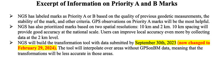
    NGS’ plans include accepting user data, but after February 29, 2024, they will not include additional GNSS and leveling data for the initial REC national adjustment and for use in building the transformation tools. In 2018, I wrote a series of GPS World newsletters that highlighted NGS’ GPS on BM program (February 2018, April 2018, June 2018, and August 2018). At that time, the GPS on BM program was very useful in the development and implementation of the hybrid geoid model GEOID18. This newsletter will provide an update on the GPS on BM Transformation Program and provide some advice on strategically selecting marks to improve the local accuracy of the NAVD 88-to-NAPGD 2022 transformation tool.

    Links to the GPSonBM Transformation Tool web map and GPSonBM Progress Dashboard are provided in NGS’ announcement. As the announcement states, the GPSonBM Transformation Web Map provides information on marks that have GNSS-derived ellipsoid heights and published NAVD 88 orthometric heights, and where there are still gaps.

    Photo:

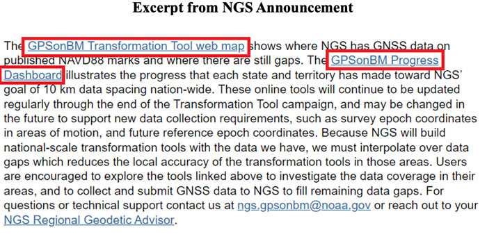
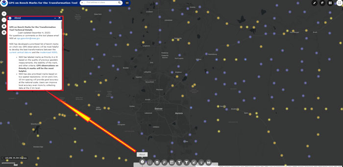
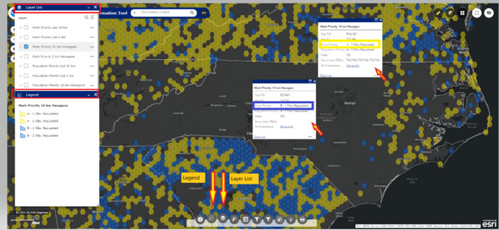
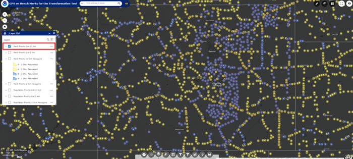
    When users click the link GPSonBM Transformation Tool Web Map, they are connected to a web map depicting a prioritized list of marks where new GNSS observations would be most helpful to the development of the transformation model between the current vertical datum (e.g., NAVD 88) and the modernized NSRS.

    NGS’ prioritized list of benchmarks are labeled as Priority A or B. Clicking on the “About” button on the webpage provides information about the priority marks. See the boxes titled “GPSonBM Transformation Tool Web Map” and “Excerpt of Information on Priority A and B Marks.”

    GPS on BM Transformation Tool Web Map. (Image: NGS website)
    GPS on BM Transformation Tool Web Map. (Image: NGS website)

    Photo:To assist users in their selection of marks, NGS developed criteria based on spatial resolution factors. See the box titled “Excerpt of Information on Spatial Resolution Factors.” As previously stated, time is running out. In my opinion, users should prioritize their GPS on BM plans based on the NGS’ criteria. I have highlighted what is important for users to consider when selecting marks.

    Photo:
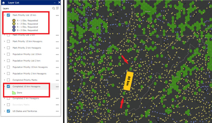
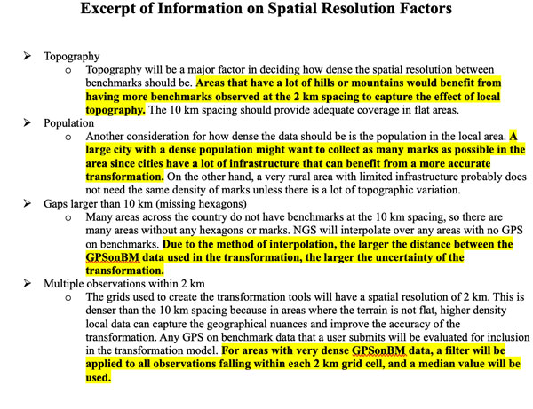
Many areas across the country do not have benchmarks at the 10 km spacing, so there are some areas without any hexagons or marks. As stated in the spatial resolution factors, NGS will interpolate over any areas with no GPS on benchmarks. In areas that have gaps larger than 10 km, that is, that are missing hexagons, I would recommend occupying several marks in each hexagon surrounding the gap to ensure that marks with valid NAVD 88 heights are part of the transformation tool. The web tool defaults to the Denver, Colorado, region when you access it but users can drag the map to an area of their interest or select a location.

    Locating marks using the GPSonBM transformation tool web map. (Image: NGS Website)
    Locating marks using the GPSonBM transformation tool web map. (Image: NGS Website)

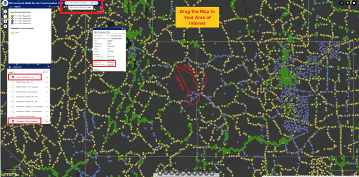
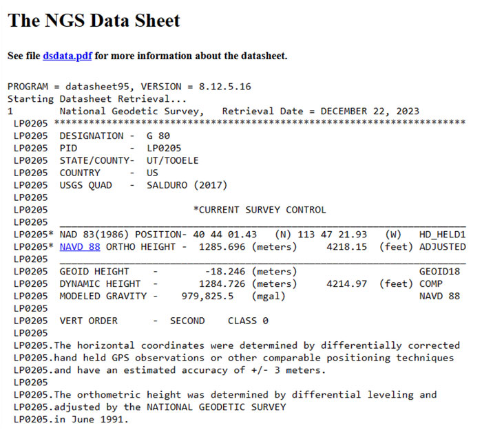
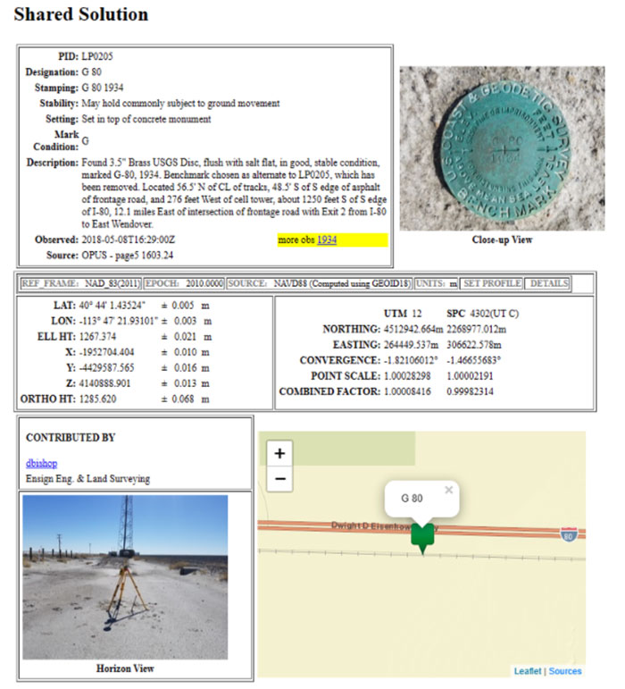
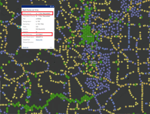
    Acquiring data in mountainous regions and areas that have large distances between completed hexagons is probably the most important for users to focus on. The box titled “Locating Marks Using the GPS on BM Transformation Tool Web Map” provide marks that need to be observed.  As an example, I have highlighted two areas that have large distances between benchmarks and completed hexagons.  In this case, it would be important to occupy a couple of marks in the highlighted locations. Clicking on a mark provides a box with the following information: Mark Priority, Population Priority, PID, Designation, Stamping, State, County, Stability code, Last Date of Recovery, Last Date of Observation, Link to NGS Datasheet, and a Link to a Shared Solution (if one exists).

    Clicking the link titled “More Info” next to Datasheet brings up the NGS datasheet for the mark, and clicking the link titled “More Info” next to Shared Solution” brings up the Shared Solution information (see the boxes titled “Mark Priority Information for Mark G 80,” “Excerpt from NGS Datasheet for Mark G 80,” and “Shared Solution for Mark G 80.”). I would recommend that State surveying organizations (and surveyors) perform this type of analysis and strategically occupy marks that fill in important gaps. There is less than two months remaining to submit data to NGS that will support the transformation tool. 

    Excerpt from NGS datasheet for Mark G 80. (Image: NGS website)
    Excerpt from NGS datasheet for Mark G 80. (Image: NGS website)
    PhotoShared solution for Mark G 80. (Image: NGS website)
    Shared solution for Mark G 80. (Image: NGS website)

    The GPSonBM Progress Dashboard illustrates the progress that each state and territory has made toward NGS’ goal of 10 km (and 2 km) data spacing nationwide.

    GPSonBM Program Dashboard. (Image: NGS website)
    GPSonBM Program Dashboard. (Image: NGS website)

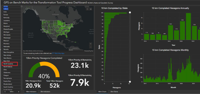
    Users can see the GPS on Benchmark information for a particular state by clicking on the name of the state on the left side of the website.

    Selection of North Carolina. (Image: NGS website)
    Selection of North Carolina. (Image: NGS website)

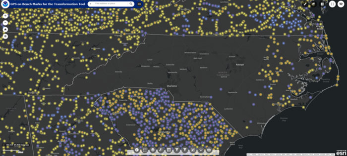
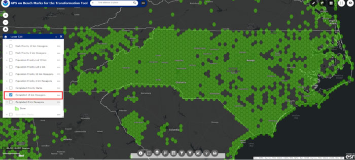
    I highlighted North Carolina because I live in that state. The map informs the users of how many 10 km priority A (89) and B (32) marks are remaining to be occupied, and the percentage completed (92%). Clicking on the link “To see remaining marks to be collected use GTT Web Map App,” located under the map, depicts the remaining marks to be collected. As you can see from the plot, North Carolina has several marks in the eastern portion of the state that still need to be occupied with GNSS.

    Status of GPS on benchmarks in North Carolina. (Image: NGS website)
    Status of GPS on benchmarks in North Carolina. (Image: NGS website)

    A nice feature of the map is the legend and layer list buttons. Also, information about the mark appears if you click on a mark.

    Example of Legend and Layer List. (Image: NGS website)
    Example of legend and layer list. (Image: NGS website)

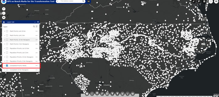
    The image below provides a list of layers that can be selected using the webtool.

    Photo:

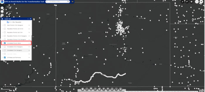
    The following image depicts marks that have been completed. As you see from the plot, North Carolina has been very active in the GPS on Benchmark program.

    Completed marks in North Carolina. (Image: NGS website)
    Completed marks in North Carolina. (Image: NGS website)

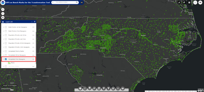
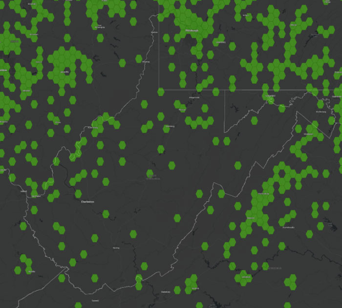
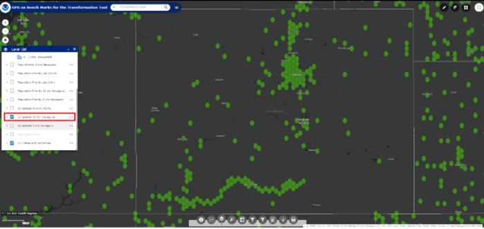
    Users can also click on the button to see which 10 km (and 2 km) hexagons have been completed (see the boxes titled “Completed 10 km Hexagons in North Carolina” and “Completed 2 km Hexagons in North Carolina”).

    Completed 10km Hexagons in North Carolina. (Image: NGS website)
    Completed 10km Hexagons in North Carolina. (Image: NGS website)
    Completed 2km Hexagons in North Carolina. (mage: NGS website)
    Completed 2km Hexagons in North Carolina. (mage: NGS website)

    The North Carolina Geodetic Survey, under the leadership of Gary Thomson, along with NC surveyors has been involved with the GPSonBM program from its inception.

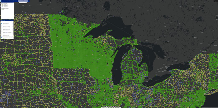
    As previously stated, the website provides the list of priority benchmarks and the status of GPS on Benchmark for each state. There are other states that have been very active in the GPS on Benchmark program such as Minnesota and Wisconsin.

    Completed 10 km Hexagons in Great Lakes Region. (Image: NGS website)
    Completed 10 km Hexagons in Great Lakes Region. (Image: NGS website)

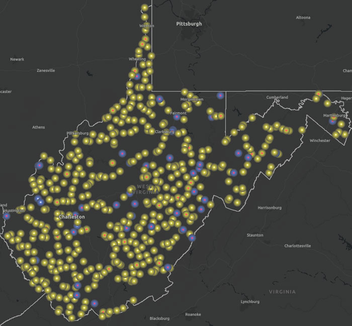
    The following images provide the GPS on Benchmark information for West Virginia.

    Status of GPS on benchmarks in West Virginia. (Image: NGS website)
    Status of GPS on benchmarks in West Virginia. (Image: NGS website)
    Completed marks in West Virginia. (NGS website)
    Completed marks in West Virginia. (NGS website)
    Completed 10 km hexagons in West Virginia. (Image: NGS)
    Completed 10 km hexagons in West Virginia. (Image: NGS)


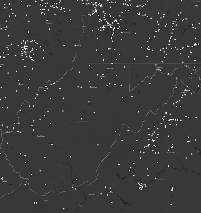
    The following image provides a plot of an area in West Virigina that highlights a region with a large gap between completed 10 km hexagons. If a user was interested in supporting the development of the transformation model in West Virigina, occupying a mark with GNSS in this area would help improve the local accuracy of the NAVD 88-to-NAPGD 2022 transformation tool.

    Overlay of completed and status of benchmarks in West Virginia. (Image: NGS website)
    Overlay of completed and status of benchmarks in West Virginia. (Image: NGS website)

    North Carolina and West Virginia are not large states compared to some western states. The boxes titled “Status of GPS on Benchmarks in Colorado,” “Completed Marks in Colorado,” “Completed 10 km Hexagons in Colorado,” and “Overlay of Completed and Status of Benchmarks in Colorado” provide the information for Colorado. Looking at the plots there appears to be many regions that could use GPS on Benchmark occupations.

    Status of GPS on benchmarks in Colorado. (Image: NGS website)
    Status of GPS on benchmarks in Colorado. (Image: NGS website)
    Completed marks in Colorado. (Image: NGS)
    Completed marks in Colorado. (Image: NGS)
    Completed 10 km hexagons in Colorado. (Image: NGS website)
    Completed 10 km hexagons in Colorado. (Image: NGS website)

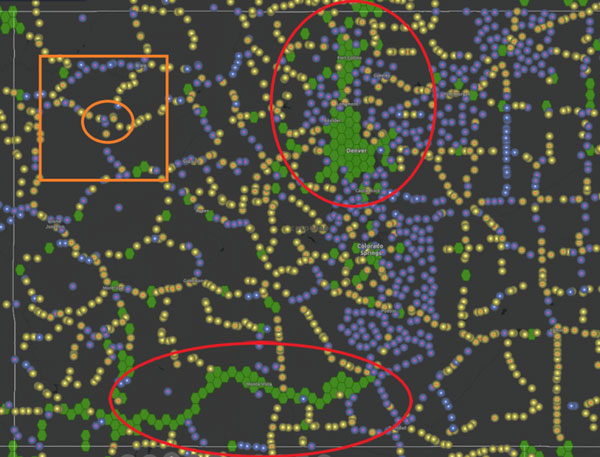
    Looking at the plot in the image below, there appear to be many marks that were occupied in populated areas such as Denver, Fort Collins, and Colorado Springs. The marks along the southern border were part of NGS’ 2017 Geoid Slope Validation Survey (GSVS) Project. The area highlighted by the orange box is an area that is lacking GPS on Benchmark occupations. The distance between the nearest completed 10 km hexagon is 60 kilometers. In other words, the two completed hexagons are more than 120 km apart. As previously stated, NGS will interpolate over any areas with no GPS on benchmarks.

    Overlay of completed and status of benchmarks in Colorado. (Image: NGS website)
    Overlay of completed and status of benchmarks in Colorado. (Image: NGS website)

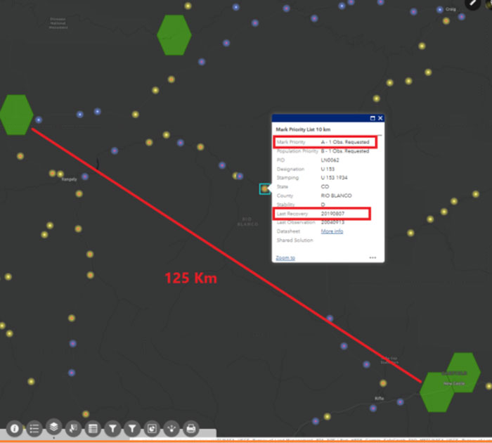
    Again, in areas that have gaps larger than 10 km with missing hexagons, I recommend occupying several marks in each hexagon surrounding the gap to ensure that marks with valid NAVD 88 heights are part of the transformation tool. To demonstrate this concept, I have selected an area in Colorado near benchmark U 153 (PID LN0062).

    Benchmark U 153 in Colorado. (Image: NGS website)
    Benchmark U 153 in Colorado. (Image: NGS website)

    The following image depicts the locations of the completed hexagons near benchmark U 153.

    Photo:

    NGS has developed web tools to assist users in the selection of marks for the program. Two web tools that I find useful are the Leveling Project Page and the Passive Mark Page. The Leveling Project Page provides information on leveling line data. Users can find information about the marks involved with a certain leveling line. There are links to the Passive Mark Page and NGS datasheets on the Leveling Project Page. My October 2020 GPS World newsletter described the Passive Mark Page web tool in more detail, and my June 2021 GPS World newsletter demonstrated the use of the tools.

    In this example, I selected U 153 because it was located between two completed 10 km hexagons that are 125 km apart. That said, looking at the information from the passive mark web tool, it appears that the published height of the benchmark is based on 1934 leveling data. That by itself is not a bad thing but the Orthometric Height Residual is very large (-23.1 cm). This implies that the difference between the GNSS-derived orthometric height using Geoid18 and the published NAVD 88 height disagreed by 23.1cm. This could be due to the movement of the mark and, in my opinion, is not a good candidate for the transformation tool.

    Photo:

    Photo:

    As previously stated, NGS’ Leveling Project Page, provides information on the benchmarks and associated data involved in a leveling line. See the box titled “Excerpt from NGS Leveling Project Page for L2577.” Users can find information about all the marks involved with a certain leveling line.


    Excerpt from NGS Leveling Project page for L2577. (Image: NGS website)
    Excerpt from NGS Leveling Project page for L2577. (Image: NGS website)
    Distance between 10km hexagons near B 383 in Colorado. (Image: NGS website)
    Distance between 10km hexagons near B 383 in Colorado. (Image: NGS website)

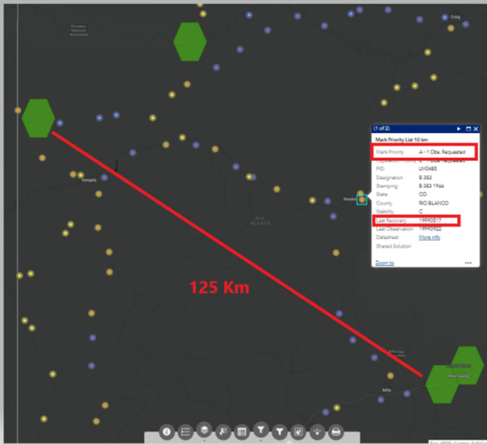
    Again, I used the Passive Mark tool to find detailed information about the mark. See the box titled “Excerpt from NGS Passive Mark Tool for B 383.” This mark was last leveled in 1966 and the Orthometric Height Residual is small (1.2 cm). This implies that the difference between the GNSS-derived orthometric height using Geoid18 and the published NAVD 88 height disagreed by 1.2 cm.

    This could be a good candidate for the GPS on BM program and the transformation tool.

    Excerpt from NGS passive mark tool for B 383. (Image: NGS)
    Excerpt from NGS passive mark tool for B 383. (Image: NGS)

    Photo:

    For completeness, I looked at another mark in the same area.

    Distance Between 10km hexagons near B 154 in Colorado. (Image: NGS website)
    Distance Between 10km hexagons near B 154 in Colorado. (Image: NGS website)

    I highlighted this mark because it was last leveled on the same 1934 leveling line as mark U 153. Unlike U 153, looking at the information provided by the Passive Mark tool for B 154 indicates that the GNSS-derived orthometric height agrees with the published leveling-derived orthometric height. The orthometric height residual is only -2.1 cm. This would be another good candidate to fill the area between the two completed hexagons.

    Photo:Photo:

    This newsletter provided some advice on strategically selecting marks to improve the local accuracy of the NAVD 88-to-NAPGD 2022 transformation tool. Again, I would recommend that state surveying organizations and surveyors perform the analysis described above and strategically occupy marks that fill in important gaps. There is less than two months remaining to submit data to NGS that will support the transformation tool.

    NGS has developed web tools such as Passive Mark Page and Leveling Project Page to assist users in identifying marks for inclusion in the development of the transformation model between the current vertical datums (e.g., NAVD 88) and the modernized NSRS.


  • USGS, Dewberry release precision lidar map of Potomac River

    USGS, Dewberry release precision lidar map of Potomac River

    Topobathymetric digital elevation model of the confluence of the Potomac and Shenandoah Rivers at Harper’s Ferry, West Virginia. (Image: USGS)
    Topobathymetric digital elevation model of the confluence of the Potomac and Shenandoah Rivers at Harper’s Ferry, West Virginia. (Image: USGS)

    The United States Geological Survey (USGS) and Dewberry, a privately held professional services firm, have jointly released a new topobathymetric lidar dataset for the Potomac River, extending from the Potomac Highlands in West Virginia to the Chesapeake Bay in Maryland.

    The survey was conducted using Teledyne Optech CZMIL SuperNova lidar system, which allowed Dewberry to successfully survey a 55-mile (88.5km) stretch of the Potomac River, spanning from Hancock, Maryland to Shepherdstown, West Virginia. The survey resulted in the acquisition of 33km² of submerged topobathymetric lidar data.

    Project deliverables included a 3D point cloud and topobathymetric digital elevation models (DEMs) for the surveyed river section. This project, the second for the Potomac River, builds on the first, which covered the area from Shepherdstown, West Virginia, to the Little Falls dam near Washington, DC. The generated maps are designed to serve as a valuable tool for predicting oil spill presence and movement in the Potomac River, supporting ICPRB’s mission to safeguard the waters and resources of the Potomac River basin through science, regional cooperation and education.

    Conducted for the USGS’s 3D Elevation Program (3DEP), the lidar survey involved collaboration with the USGS Earth Resources Observation and Science Center (EROS), National Geospatial Program (NGP) and Eastern Ecological Science Center (EESC) programs, along with the Interstate Commission on the Potomac River (ICPRB).

  • ASPRS approves edition 2 of the ASPRS Positional Accuracy Standards for Digital Geospatial Data

    ASPRS approves edition 2 of the ASPRS Positional Accuracy Standards for Digital Geospatial Data

    On Oct. 26, 2023, I participated in an American Society for Photogrammetry and Remote Sensing (ASPRS) Pacific Southwest Region Fall Technical webinar. The webinar provided an overview of the ASPRS Positional Accuracy Standards for Digital Geospatial Data (Edition 2, Version 1.0 – August 2023). The document can be downloaded here.

    ASPRS Webinar Announcement. (Image: ASPRS)
    ASPRS Webinar Announcement. (Image: ASPRS)

    I also participated — virtually — in the Nov. 2, 2023, California Spatial Reference Center (CSRC) Coordinating Council fall meeting where Dr. Riadh Munjy, California State University, Fresno, discussed the revisions to the ASPRS Positional Accuracy Standards for Geospatial Data.

    The most significant changes introduced in this second edition of the standards include:

    1. Elimination of references to the 95% confidence level as an accuracy measure.
    2. Relaxation of the accuracy requirement for ground control and checkpoints.
    3. Consideration of survey checkpoint accuracy when computing final product accuracy.
    4. Removal of the pass/fail requirement for Vegetated Vertical Accuracy (VVA) for lidar data.
    5. Increase the minimum number of checkpoints required for product accuracy assessment from 20 to 30.
    6. Limiting the maximum number of checkpoints for large projects to 120.
    7. Introduction of a new term: three-dimensional positional accuracy.
    8. Addition of Best Practices and Guidelines Addenda for:
      1. General Best Practices and Guidelines
      2. Field Surveying of Ground Control and Checkpoints
      3. Mapping with Photogrammetry
      4. Mapping with Lidar
      5. Mapping with UAS

    As outlined above, Edition 2 contains Best Practices and Guidelines for (1) General Best Practices and Guidelines and (2) Field Surveying of Ground Control and Checkpoints. The three addenda listed in the table of contents: Mapping with Photogrammetry, Mapping with Lidar, and Mapping with UAS will be available for public comment later, and will be added to Edition 2, Version 2.0.

    Dr. Abdullah informed me that these addenda are on track to be put out for public comments during December 2023, therefore he believes they will probably be published in January or February 2024. The box titled “Summary of Significant Changes in Edition 2” provides the changes with the reason and justification for each change. The document can be downloaded from ASPRS here.Photo:Photo:Photo:Photo:Photo:

    One of the changes is to relax the accuracy requirement for ground control and checkpoints. At first glance, this seems like the wrong thing to do. However, after understanding the justification, the requirement for ground truth still needs to be at least twice as accurate as the product.

    Both Dr. Abdullah and Dr. Munjy’s emphasized in their presentations that the current accuracy requirements for ground controls in photogrammetric work of four-times better than the produced products, and the checkpoint accuracy requirement is three-times better than the assessed product. This makes it difficult, if it is not impossible, to use RTK-based techniques for this type of surveying. This by itself is not the reason for the change. During Dr. Abdullah’s presentation, he provided the following reasons for the change:

    1. “Experience taught us that the requirements of four-times and three-times adopted in edition 1 of the standards are excessive and too restrictive, partly due to the reason outlined in (b) below.
    2. Today’s sensors, software, and processing methodology are more accurate and the room for errors in the product is diminishing, therefore we do not need a safety factor of 3 or 4 to obtain accurate products.
    3. Increasing demand for higher accuracy geospatial products.”

    The new standards now factor in the accuracy of the survey checkpoints when determining the accuracy of the product. During Dr. Abdullah’s presentation, he provided the following reason for the change, “As we are producing more accurate products, errors in surveying techniques of the checkpoints used to assess product accuracy, although small, can no longer be neglected and it should be represented in computing the product accuracy.” He also highlighted that, “As product accuracy increases, the impact of error in checkpoints on the computed product accuracy increases.” The document provides equations used to compute the values. See below.

    Equations for Checkpoints. (Image: ASPRS)

    Photo:

    A very significant change, in my opinion, is the removal of the standards for Vegetated Vertical Accuracy (VVA) for lidar data. See below.

    Photo:

    Photo:
    VVA not used as a criterion for acceptance. (Image: ASPRS)

    I am not sure I agree with the reasoning, but I understand why it was done. GNSS-based surveys do not perform well in vegetated areas, and this is the technology used to validate the non-vegetated vertical accuracies (NVA). That said, there are non-GNSS technologies — sometimes denoted as traditional surveying methods — that could be used to validate VVA, so this seems like an elimination of a requirement based on the limitation of a particular technology.

    Traditional surveying methods that use geodetic levels, theodolites, and total stations to measure distances, angles, and heights are still used by surveyors to perform certain projects. Since there are other surveying methods that could be used for evaluating the VVA, it does not seem like a valid reason for a change.

    The ASPRS standards does state that, “for projects where vegetated terrain is dominant, the data producer and the client may agree on an acceptable threshold for the VVA.” Therefore, the client can require the surveyor to meet a specific accuracy level for vegetated areas. I am sure this was discussed during the working meeting, so I leave it to the experts to make the appropriate decisions and recommendations.

    Finally, it should be noted that, as discussed above, the new ASPRS standards eliminated the reference to the 95% confidence level as an accuracy measure. The document provides the following statement about the National Standard for Spatial Data Accuracy (NSSDA):

    “The National Standard for Spatial Data Accuracy (NSSDA) documents the equations for the computation of RMSEX, RMSEY, RMSER and RMSEZ, as well as horizontal (radial) and vertical accuracies at the 95% confidence levels — AccuracyR and AccuracyZ, respectively. These statistics assume that errors approximate a normal error distribution and that the mean error is small relative to the target accuracy. The ASPRS Positional Accuracy Standards for Digital Geospatial Data reporting methodology is based on RMSE alone, and thus differs from the NSSDA reporting methodology. Additionally, these Standards include error inherited from ground control and checkpoints in the computed final product accuracy.”

    Appendix D of the ASPRS document provides the equations with an example for computing the accuracy statistics. The document also has a section with examples for users who wish to relate the ASPRS 2023 Standards to the FGDC National Standard for Spatial Data Accuracy (NSSDA).

    Dr. Munjy ended his presentation at the CSRS 2023 fall meeting with the following statements:

    “ASPRS Accuracy Standards 2023 have become more aligned with science and statistical theory,” and “These Standards are intended to be a living document which can be updated in future editions to reflect changing technologies and user needs.”

    I would encourage all users to download the document to better understand the changes and reasons for the changes. It can be downloaded here.

  • They used GPS even before it was fully built: The adoption of GPS by surveyors

    They used GPS even before it was fully built: The adoption of GPS by surveyors

    Photo: stock_colors/iStock/Getty Images Plus/Getty Images
    Image: stock_colors/iStock/Getty Images Plus/Getty Images

    The Global Positioning System (GPS) project started 50 years ago, in 1973. I was fortunate to be part of incorporating GPS into the National Spatial Reference System (NSRS) when I worked for the National Geodetic Survey (NGS). GPS was not considered operational until 1993, but NGS started performing GPS surveys in 1983. Geodetic control surveys that formerly took six to 12 months to perform using classical methods could be performed with GPS in a few weeks using fewer personnel and resources. It changed the way NGS and others performed their surveying operations.

    While one group in NGS was developing programs to evaluate and compute coordinates using GPS, another NGS group was completing the readjustment of the North American Datum of 1983 [NAD83 (1986)]. The analysis of GPS indicated that some of the latitude and longitude values estimated using GPS did not agree with the published NAD83 coordinates. The classical techniques used a triangulateration process (involving angles and distances) that required several triangles to connect two stations that were not intervisible. GPS, on the other hand, could directly measure the distance between the two stations, resulting in more accurate coordinate differences.

    To support surveyors, NGS, working with other federal agencies under the auspices of the Federal Geodetic Control Subcommittee (FGCS), developed a GPS test network in the Washington, D.C., area to demonstrate whether a specific manufacturer’s GPS receiver and associated geodetic post-processing software was an accurate relative positioning satellite survey system. This facilitated the use of GPS for incorporating geodetic control in the NSRS. As mentioned above, GPS surveys exposed many inconsistencies between existing NAD83 (1986) control. Organizations such as NGS and state transportation departments that performed control surveys used GPS as soon as equipment met the federal testing requirements because it was more efficient and cost-effective than classical techniques. This led individual states to perform statewide geodetic network projects to upgrade their NAD 83 (1986) coordinates. These surveys were ultimately designated as High Accuracy Reference Networks (HARN).

    In the beginning, the attitude of the individual surveyor accepting GPS was one of “trust after verifying.” Many surveyors considered it to be a “black box” that could not be trusted. Surveyors were accustomed to having angles and distances they could write down and check the results. Also, there were some key challenges and limitations of using GPS for surveying in the early days. This included the cost and size of the equipment, the peripheral devices required, the power requirements (including 12v car batteries and generators), “black box” computer processing software, obstructions near monuments, and limited visibility of GPS satellites.

    Prior to GPS becoming fully operational, some surveys had to be performed in the middle of the night to have four or more satellites visible during the observing session. This required a significant amount of technical planning, which sometimes required complicated logistics for coordinating observing sessions. Also, at that time, most private surveyors did not perform control projects, so even though GPS may be more accurate, it was not more cost-effective than classical techniques for their typical projects.

    Over time, after GPS became operational, more surveyors (and other professionals) embraced using GPS after the cost of receivers decreased, user-friendly processing software became available (e.g., NGS OPUS), Continuously Operating Reference Stations were densified (e.g., NOAA CORS), and statewide Real-Time Networks (RTN) were established (e.g., North Carolina RTN). GPS technology now underpins many sciences, large areas of engineering (such as driverless vehicles and UAVs), navigation, and precision agriculture. GPS (today GNSS) and its applications have changed the way surveyors and geospatial users perform their work, and the world has seen the development of applications that were not ever imagined 50 years ago.

  • Point One Navigation expands location solutions to cover Great Britain

    Point One Navigation expands location solutions to cover Great Britain

    Image: Point One Navigation
    Image: Point One Navigation

    Point One Navigation has integrated Ordnance Survey base stations into the Polaris Network, which is designed to improve accuracy, precision, reliability and interoperability in the UK. The solutions aim to aid in applications such as advanced driver assistance (ADAS), robotics, mapping and more.  

    Polaris is a real time kinematic (RTK) corrections network that offers cm-level accurate GNSS positioning. Polaris’ global RTK network now includes the entire United States, EU, Australia, Canada and the UK. 

    Existing Polaris customers can utilize the UK integration immediately, at no additional cost. 

    This technology is complemented by the company’s FusionEngine software, which further integrates inertial measurement, wheel odometry and additional sensors to achieve the desired level of precision, even in the absence of satellite signals.  

    Polaris supports all major GNSS constellations and has a dense global network of base stations, which offers improved precision acquisition time in more places, the company says. The network supports all modern navigation signals across all mobile networks. 

    According to Point One, it is the first localization service with a modern GraphQL-based API, which aims to improve the integration of Polaris RTK into developer-built applications. It can be used by software developers to integrate RTK into demanding applications, including industrial autonomy, precision agriculture, logistics and delivery, robots and ADAS.  

    It will support State Space Representation (SSR) corrections delivered by L-band satellites in early 2024, the company says, which will allow for operations to continue in the absence of cellular networks or in bandwidth constrained applications.   

  • RIEGL launches three airborne survey systems

    RIEGL launches three airborne survey systems

    RIEGL has released three airborne survey products. The three systems are designed to enhance sensor performances and capabilities in various segments, from terrestrial, to mobile and airborne applications.

    RIEGL VQX-2 – Helicopter pod for airborne surveying

    Image: RIEGL
    Image: RIEGL

    The VQX-2 helicopter pod is  designed for airborne data collection. It integrates a RIEGL laser scanner, a high-performance IMU/GNSS unit, and up to five cameras. It also can be easily mounted and dismounted onto UAVs.

    The VQX-2 can be used in a variety of applications such as corridor mapping, surveying large areas from high altitudes, monitoring glaciers and landslides and more. The solution includes the corresponding cabling; a “Minor Change Approval” is already available for Airbus Helicopters AS350 series helicopters.

    RIEGL VQ-680 OEM – Airborne lidar scanning module for OEM integration

    Image: RIEGL
    Image: RIEGL

    The VQ-680 compact airborne lidar scanner OEM is designed to be integrated with large-format cameras or other sensors in complex hybrid system solutions.

    The module can be mounted inside a camera system connected to the IMU/GNSS system and various camera modules through a sturdy mechanical interface. It also has laser pulse repetition rates of up to 2.4 MHz and 2 million measurements per second.

    The VQ-680 is ideal for large-scale applications in urban mapping, forestry and power line surveying, the company says. With a wide field view of 60º andRIEGL’s nadir/forward/backward (NFB) scanning, the system offers five scan directions up to ± 20º. This technology provides users exceptional coverage of vertical structures such as building facades or power poles at high accuracy.  

    The OEM’s sister type, the VQ-680, is offered as a high-end airborne lidar scanner that offers the full range of performance in a compact and lightweight scanner. This scanner can be coupled with up to six high-resolution RGB/NIR cameras and mounted onto appropriate aircraft hatches with or without using stabilized platforms. 

    RIEGL VUX-180-24 –UAV lidar sensor for high-speed surveying missions 

    Image: RIEGL
    Image: RIEGL

    The VUX-180-24 offers a wide field of view of 75º and a high pulse repetition rate of up to 2.4 MHz. These features – in combination with an increased scan speed of up to 800 lines per second – make it suitable for high-speed surveying missions and applications where an optimal line and point distribution is required.

    Typical applications include mapping and monitoring of critical infrastructure such as power lines, railway tracks, pipelines, and runways. The  VUX-180-24 provides mechanical and electrical interfaces for IMU/GNSS integration and up to five external cameras. For smooth and straight forward data storage, an internal SSD memory with 2 TByte storage capacity and a removable CFast memory card are available.

    This sensor can be coupled with RIEGL’s VUX-120, VU-160, and VUX-240 series UAVs. The system is available as a stand-alone sensor or in various fully integrated laser scanning system configurations with IMU/GNSS systems and optional cameras.

  • ComNav introduces 3D laser scanning system

    ComNav introduces 3D laser scanning system


    Image: ComNav Technology
    Image: ComNav Technology

    ComNav Technology has released the LS300 3D laser scanning measurement system.

    The scanner utilizes simultaneous localization and mapping (SLAM) technology, and advanced real time and mapping techniques. It operates autonomously, independent of GNSS positioning, which makes it ideal for harsh conditions in both indoor and outdoor environments.

    LS300 includes a 120-meter working range and a high sampling rate of 0.32 million points per second. Its point cloud accuracy is designed to perform in low reflectivity extended-range mode. The system is compatible with specialized kits, including the handheld form, back kit, car-mount and UAV kit.

    Image: ComNav Technology
    Image: ComNav Technology

    The handheld mode is best suited for navigating narrow tunnels and large venues, while the backpack is designed for outdoor environments. The car mount can rapidly scan roadside facilities, and the UAV kit seamlessly pairs with the DJI M300 for aerial control. The LS 300 is suitable for a variety of applications, including smart city, digitization of underground facilities, geology, surveying and mapping, agriculture, mining and forestry.

    The scanner uses a unique hybrid HSL technology. This allows for preliminary processing during the scanning process, which aims to accelerates the collection of high-precision data and expedites data processing. It offers real-time viewing of point cloud data through a mobile application and supports multiple interaction modes.

    By using data processing software specifically designed and developed for the LS series by ComNav, users can handle large volumes of point cloud data and simplify complex tasks, including point cloud denoising, point cloud splicing, shadow rendering, coordinate transformation, automatic horizontal plane fitting, automatic point cloud data report generation, forward photography, and point cloud encapsulation. This allows users to efficiently process intricate point cloud data, resulting in precise measurement and modeling outcomes.

    During data post-processing, users can input absolute coordinates of control points, which allows these control points to make comprehensive adjustments to the data and improve scanning data accuracy.

    The LS300 also incorporates a redundant battery design with two hot-swappable batteries, designed for prolonged operation without frequent charging or interruptions. This innovative approach contributes to enhanced safety, reliability, and efficiency, the company says.

  • CHC Navigation introduces USV for bathymetric surveys

    CHC Navigation introduces USV for bathymetric surveys

    Image: CHCNAV
    Image: CHCNAV

    CHC Navigation (CHCNAV) has launched the Apache 3 Pro, a compact hydrographic uncrewed surface vessel (USV) designed for autonomous bathymetric surveys in shallow waters. A lightweight carbon fiber hull with IP67-rated ingress protection and semi-recessed motor provides durability and maneuverability.

    Featuring CHCNAV’s GNSS RTK + inertial navigation sensor, the Apache 3 Pro offers consistent, high-precision positioning and heading data even when navigating under bridges or in areas with obstructed satellite signals. The built-in CHCNAV D270 echosounder allows for reliable depth measurement from 0.2 to 40 meters.

    The Apache 3 Pro is also equipped with a millimeter-wave radar system that detects obstacles within a wide 110° field of view. When an obstacle is encountered, the USV autonomously charts a new course to safely navigate around it. The vessel uses both 4G and 2.4GHz networks to facilitate effective data transfer.

    Weighing only 10 kg, it features a lightweight macromolecular polyester carbon fiber and Kevlar composite hull for improved resilience. Even with a fully integrated payload, the USV can be easily deployed and controlled by a single operator in a variety of environmental conditions.

    The Apache 3 Pro ensures reliable communications through its integrated SIM and network bridge with automatic switching. It also features seamless cloud-based remote monitoring that offers real-time status updates to enhance control and security. Its semi-recessed brushless internal rotor motors minimize drafts, which can improve the USV’s maneuverability in varying water depths.

  • Using GNSS Phase Reflectometry on Maui’s Haleakalā

    Using GNSS Phase Reflectometry on Maui’s Haleakalā

    Read Richard Langley’s introduction to this article:Innovation Insights: Science in paradise”


    Originally developed for navigation and timing applications, signals from global navigation satellite systems (GNSS) are now commonly used for geophysical remote sensing applications, including observation of Earth’s surface and atmosphere using near sea-level ground stations as well as mountaintop, airborne and spaceborne platforms. GNSS reflectometry (abbreviated GNSS-R), which is the technique of using reflected signals to measure properties of Earth’s surface, has been a growing area of research and application for GNSS remote sensing. Notably, the Cyclone Global Navigation Satellite System (CYGNSS) satellite mission produces delay-Doppler maps (DDMs) that are used to monitor ocean surface wind speeds during hurricanes. Meanwhile, terrestrial and airborne GNSS-R has been used to monitor soil moisture, snow depth and vegetation growth. One area of increasing interest is precision reflectometry using signal carrier-phase measurements. The first attempt to perform precision (phase) altimetry over sea ice using GPS reflectometry measurements from the low-Earth orbiting TechDemoSat-1 was reported by researchers in 2017. Subsequently, researchers demonstrated the use of reflections collected by a Spire satellite to perform altimetry over Hudson Bay and the Java Sea and how reflections off ice in the polar regions can be used to measure ionospheric total electron content over the polar caps. While these demonstrations of GNSS-R for precision carrier-phase-based reflectometry are promising, more work needs to be done to characterize when carrier-based altimetry is feasible and what challenges it faces.

    To study the challenges associated with processing reflected and low-elevation-angle radio occultation signals, the University of Colorado (CU) Boulder Satellite Navigation and Sensing (SeNSe) Laboratory has deployed a GNSS data collection site on top of Mount Haleakalā on the island of Maui, Hawaii. Recent collection campaigns aim to use this site as a testbed for GNSS-R algorithms that utilize multi-frequency and multi-polarization measurements. Previously, we carried out delay map processing for left-hand circular (LHC) and right-hand circular (RHC) polarizations for L1 and L2 GPS signals. Those results validate the open-loop processing methodology and provide an initial assessment of the data quality. We observed that the received reflected signals show deep and rapid fading in amplitude. In the work reported in this article, we extend our assessment to triple-frequency GPS (L1CA, L2C, L5Q) signals and document our methodology for extraction of the signal carrier phase. Our initial results indicate that coherent signal phase extraction is challenging, and may not be feasible for this particular experiment setup. We discuss ways in which the experiment may be improved for the purpose of obtaining coherent ocean surface reflections in the future.

    EXPERIMENT BACKGROUND

    The current form of the CU SeNSe Lab Mount Haleakalā GNSS experiment was deployed in June 2020. It consists of a side-facing dual-polarization horn antenna, which is shown in the left panel of FIGURE 1, along with a zenith-facing reference antenna. The horizontally- and vertically-polarized wideband signals from the horn antenna are fed into front-end hardware and are combined using 90-degree phase combiners to form LHC and RHC polarized signals, which are then recorded by a set of Ettus Universal Software Radio Peripherals (USRPs). Meanwhile, the signal from the reference antenna is sent to a Septentrio PolaRxS receiver. The right panel in Figure 1 illustrates the system setup. Note that the Septentrio onboard oven-controlled crystal oscillator is used to drive the USRPs. This allows us to use the Septentrio outputs to estimate the receiver clock variations and use them in the receiver clock component of our open-loop models, which we discuss below.

    Figure 1 The side-facing horn antenna in its radome enclosure (left panel) and the hardware block diagram of the data collection system (right panel). (All figures provided by the authors)
    Figure 1: The side-facing horn antenna in its radome enclosure (left panel) and the hardware block diagram of the data collection system (right panel). (All figures provided by the authors)

    Each USRP can record up to four signals at two different mixdown frequencies, allowing for recording of both the RHC and LHC polarized signals on up to four different bands. The first USRP records the L1 and L2 bands with center frequencies at 1575.42 and 1227.6 MHz, respectively, at a bandwidth of 5 MHz. The second USRP records the L5 and E6/B3 bands at center frequencies of 1176.45 and 1271.25 MHz and at a 20 MHz bandwidth. TABLE 1 lists the IDs for each receive channel along with its corresponding band, polarization and sampling rate. Note that the recorded signals covering the E6 band also capture BeiDou B3 signals, but we restrict our analysis to GPS L1, L2 and L5 signals in this article. The samples from these USRPs are written to disk along with the Septentrio Binary Format (SBF) output of the PolaRxS receiver.

    Table 1 Receiver IDs with corresponding band and polarization.
    Table 1: Receiver IDs with corresponding band and polarization.

    Starting in June 2021, periodic collections were taken for around one hour at a time, which is about the amount of time it takes for a GPS satellite to pass from an elevation angle of 0 degrees to one of more than 20 degrees. The collection times were adjusted to target the passes of satellites whose specular reflection point passed within the azimuthal range of the horn antenna, which faces roughly to the south and has a beam width of around 60 degrees. FIGURE 2 summarizes the available datasets from the first month of collections. The right-most panels of FIGURE 3 show examples of the specular track for GPS PRN 6 as it sets over the horizon on June 13, 2022, at around 12:00-13:00 UT. This is the pass on which we focus in this work, since PRN 6 transmits the L1CA, L2C and L5 signals and consistently had a specular point in our region of interest.

    Figure 2 Available data during the first month of collections. The average significant wave height in the region south of Haleakalā is also plotted. Numbers near the bottom indicate the datasets analyzed for this article.
    Figure 2: Available data during the first month of collections. The average significant wave height in the region south of Haleakalā is also plotted. Numbers near the bottom indicate the datasets analyzed for this article.

    METHODOLOGY

    Our processing method for open-loop tracking of the reflected GNSS signals is based on our previous work in which we produced DDMs and delay maps of the signal-to-noise ratio (SNR) measurements for multiple signal frequencies and received polarizations.

    Pseudorange Model. We start by generating a model of the pseudorange for both the direct and reflected signal. The model only needs to be accurate down to the chip level, since we correlate across several chips of delay for the received signals. Setting a somewhat arbitrary accuracy requirement of 0.5 chips (equivalent to a delay of around 150 meters for L1CA/L2C or 15 meters for L5 signals), allows us to ignore path delays from the ionosphere and troposphere, which should only account for up to several meters of delay. The model has three terms that we estimate relative to GPS System Time (GPST): the receiver clock error, the satellite transmitter clock error and the geometric range. We use a surveyed position of the horn antenna along with International GNSS Service precise orbit and clock products for the transmitter clock error and positions. These allow us to compute the transmitter clock error and path delay for the direct signal. The reflected signal path delay can be found by computing the specular reflection point on the WGS84 ellipsoid and adding the distances from the transmitter to the specular point and the specular point to the receiver. The remaining term to estimate is the receiver clock error. Recall that our USRPs are driven by the Septentrio internal oscillator. Therefore, the clock error in Septentrio measurements is associated with variations in the reference oscillator for the USRPs. We utilize a geodetic detrending technique to estimate these clock variations and apply them to our pseudorange model. To construct the full receiver clock error, we estimate the time-alignment of the samples near the beginning of the collections to GPST by tracking one minute of a strong, mid-elevation-angle satellite and decoding its timing information. This provides us with an estimate of GPST at the start of the file, which we can use to construct a full estimate of the GPST at any sample in the file. Also, given our pseudorange model, we can find the received code phase and the Doppler frequency.

    Figure 3 Example of delay maps from GPS PRN 6. The panels to the left show delay maps for the L1CA, L2C and L5 signals, both RHC and LHC polarizations. The bottom panel shows the corresponding elevation angle over the duration of the pass. The maps to the right show the specular point location during the pass, along with a contour of the WW3 model for significant wave height and swell-significant wave height.
    Figure 3: Example of delay maps from GPS PRN 6. The panels to the left show delay maps for the L1CA, L2C and L5 signals, both RHC and LHC polarizations. The bottom panel shows the corresponding elevation angle over the duration of the pass. The maps to the right show the specular point location during the pass, along with a contour of the WW3 model for significant wave height and swell-significant wave height.

    Signal Correlation. Using the established code phase and Doppler models, we generate correlations for both reflected and direct signals. We correlate a reference signal over each 1-millisecond interval, and for sanity-checking purposes, we compute correlations over ± 3 chips at 0.5 chip spacing. This results in in-phase and quadrature (I/Q) correlation outputs every 1 millisecond. The left panels in Figure 3 show examples of the processed reflected signals for RHC and LHC polarization L1CA, L2C and L5Q signals from PRN 6 on June 13, 2021, at 12:00-13:00 UT. Note that as the satellite sets, at around 4 degrees elevation angle, the reflected signals merge with the stronger direct signal on the L1 and L2 signals. This happens later on L5 due to its higher bandwidth. We use the 0.0 chip bin to obtain I/Q outputs for carrier-phase processing for L1 and L2. For L5, we use the 0.0, -0.5, or -1.0 chip bin to account for model mismatch toward the end of the file.

    Signal Fading and the WW3 Ocean Model. An eventual goal of the Haleakalā reflectometry experiment is to compare the characteristics of processed reflected signals with the ocean surface parameters near the specular point and glistening zone. To this end, we have incorporated data from the Hawaii regional WaveWatcher 3 (WW3) model. The model outputs information about wave height, direction and period due to both wind and swell, and has a resolution of around 5 kilometers. The data from this model is available in NetCDF format from several web services. The right panels of Figure 3 show contours of the wind- and swell-significant wave height in the South Haleakalā region. Meanwhile, note that the reflected signals (left panels) show high variability in the received power throughout the duration of the collection. While we hoped to be able to immediately observe a correlation between these wave parameters and the power fluctuations, it is clear that we need additional processing to tease out such a signal, and the changing satellite geometry will likely make this difficult to observe and validate. Even still, our results at the end of this article will show that there is likely some correlation between fading and wind parameters, though to what extent is unknown. Finally, note that the LHC polarizations (RX6, RX8, RX2) show much stronger reflected signals than the RHC polarizations. Since we are interested in processing the phase for the reflected signals, we report exclusively on the use of the LHC polarization signals in the rest of this article.

    Carrier-Phase Processing. Once the correlations are performed, we take the I/Q correlations for both direct and reflected signals and process them to retrieve the cleaned reflected signal phase. The first series of steps in this process involve processing the direct signal to determine navigation / overlay symbol alignment and to estimate any residual phase fluctuations, which are mostly due to unmodeled receiver clock fluctuations. FIGURE 4 illustrates this process for the L1CA signal. The raw I/Q correlations are shown in the top panel. To these we apply a Costas phase-lock loop (PLL) to track the residual phase fluctuations without being sensitive to navigation / overlay symbol transitions. Next, we remove these residual phase fluctuations to obtain the detrended I/Q values.

    Figure 4 The I/Q data cleaning process for the L1CA direct signal.
    Figure 4: The I/Q data cleaning process for the L1CA direct signal.

    As shown in the second panel, these quadrature components of the detrended I/Q values are centered at zero while the in-phase component now shows the data bits / overlay symbols. We use the detrended I/Q values to estimate the navigation bit sequence on the L1CA and L2C signals. Likewise, we estimate the alignment of the Neumann-Hoffmann overlay sequence for the L5 signal. Finally, we wipe off the estimated data bits or overlay sequence to verify the procedure. The results of wiping off the estimated navigation bits for the L1CA signal are shown in the third panel of Figure 4.

    Having obtained the residual phase fluctuations and navigation / overlay symbols for the direct signal, we next apply these to clean up the reflected signal. Specifically, we remove residual phase fluctuations from the raw reflected signal I/Q values and then wipe off the corresponding navigation bits or overlay code. FIGURE 5 shows an example of the reflected I/Q data before and after this procedure. The navigation bits are clearly removed, but the reflected signal still shows fairly significant fluctuations in the cleaned I/Q values. It is from these values that we hope to extract the residual reflected signal phase.

    Figure 5 The reflected signal raw I/Q (top) and the I/Q after detrending and wiping off navigation bits for the L1CA signal.
    Figure 5: The reflected signal raw I/Q (top) and the I/Q after detrending and wiping off navigation bits for the L1CA signal.

    Under coherent conditions, the phase of the clean reflected I/Q data should contain only the unmodeled effects, including any signature of ocean surface height variation. However, the effect of multipath due to the rough ocean surface causes fluctuations in the received signal amplitude and phase, and can additionally cause cycle slips when we unwrap the phase. To filter out these cycle slips, we apply our simultaneous cycle slip and noise filtering (SCANF) method, which is essentially just a Kalman filter PLL with an additional step that tries to estimate and remove cycle slips. The figures in the next section show the results of applying this entire procedure to the reflected signals. The black and blue lines show the phase before and after applying SCANF. The reflected signal I/Q SNR is also included for reference. Note how the jumps in the black line coincide with SNR fades, and the blue line effectively recreates the phase trend of the black line without these jumps. This is good qualitative evidence that the SCANF algorithm was effective.

    RESULTS

    FIGURES 6, 7, 8, 9, 10, and 11 show the reflected signal SNR and phase for GPS PRN 6 on 6 different days. Note that these days correspond to the marked days in Figure 2, from which we observe that the wind-significant wave height is relatively high on days 1, 5, and 6, moderate on days 2 and 3, and relatively low on day 4. We noticed that the SNR fluctuations on days 1, 5, and 6 are comparatively more frequent than on other days, which we believe may be a signature of the ocean surface conditions. A more detailed analysis of this result is a topic for our future work.

    Figure 6 Reflected signal residual phase before (blue) and after (black) applying the SCANF filtering for the June 11, 2021 dataset. Amplitude and phase are shown in alternating panels for L1CA, L2C and L5 respectively.
    Figure 6: Reflected signal residual phase before (blue) and after (black) applying the SCANF filtering for the June 11, 2021 dataset. Amplitude and phase are shown in alternating panels for L1CA, L2C and L5 respectively.
    Figure 7: Phase processing results for June 13, 2021.
    Figure 7: Phase processing results for June 13, 2021.

    Overall, we observe that the phase trend is not consistent across the three signals (L1CA, L2C, L5) for any of the days. With all the multipath signatures in the cleaned reflected signal, it was uncertain whether the extracted phase will be useful for applications such as ocean surface altimetry, and these qualitative results suggest that they probably will not be. However, season and hours of the day that were processed for our work discussed in this article are very limited. It is possible that processing more data will shed further insight onto whether the reflected signal phase is usable in this experiment.

    Figure 8 Phase processing results for June 21, 2021.
    Figure 8 Phase processing results for June 21, 2021.
    Figure 9 Phase processing results for June 25, 2021.
    Figure 9: Phase processing results for June 25, 2021.

    ACKNOWLEDGMENTS

    The Haleakalā data collection system has been established with support from the University of Hawaii Institute of Astronomy, and the Air Force Research Laboratory. The authors appreciate the assistance from Michael Maberry, Rob Ratkowski, Daniel O’Gara, Craig Foreman, Frank van Graas and Neeraj Pujara. This research is funded by a subaward from the National Oceanic and Atmospheric Administration through the University Corporation for Atmospheric Research to CU Boulder and with partial funding support from the NASA Commercial Smallsat Data Acquisition program.

    This article is based on the paper “Initial Carrier Phase Processing for the Haleakala Mountaintop GNSS-R Experiment” presented at ION ITM 2023, the 2023 International Technical Meeting of the Institute of Navigation, Long Beach, California, Jan. 23–26, 2023.

    Figure 10 Phase processing results for July 1, 2021.
    Figure 10: Phase processing results for July 1, 2021.
    Figure 11 Phase processing results for July 5, 2021.
    Figure 11: Phase processing results for July 5, 2021.

    BRIAN BREITSCH is a postdoctoral fellow at the University of Colorado (CU) Boulder, where he received his Ph.D. in aerospace engineering sciences.
    JADE MORTON is a professor in the Ann and H.J. Smead Department of Aerospace Engineering Sciences and the director of the Colorado Center for Astrodynamics Research at CU Boulder.

  • Trimble partners with HALO Trust for landmine clearance in Ukraine

    Trimble partners with HALO Trust for landmine clearance in Ukraine

    Image: Trimble
    Image: Trimble

    Trimble has partnered with HALO Trust, a landmine-clearing non-profit organization, to help expand its demining operations across Ukraine.

    The grant from the Trimble Foundation Fund will focus on strengthening the HALO Trust’s ability to locate and remove landmines, unexploded ordnance and other explosive hazards from civilian areas to create safer communities. In addition, it will allow HALO to support the Ukrainian national authorities in planning and coordinating landmine clearance activities by streamlining the mapping and data flow from the operational teams in the field to the national database.

    The Russian invasion of Ukraine has left areas of the country contaminated with landmines, unexploded ordnance and improvised explosive devices. These hazards block access to farmland, impede reconstruction efforts, prevent displaced persons from returning to their homes and continue to hinder the safety of Ukrainian civilians. The Ukrainian government estimates that 174,000km2 of the country’s land may be contaminated.

    More than a thousand HALO staff members are active daily, both to clear explosives in critical priority areas and to recruit and train hundreds of new staff members to help keep communities safe from dangerous weapons left behind.

    Surveying and mapping technology has played a significant role in the success of HALO’s operations around the world, including in Ukraine. Over the last six years, Trimble R1 and Trimble R2 GNSS receivers along with Esri ArcGIS Survey123 software have been used by HALO to identify and clear landmines.

    Trimble’s Geospatial and Positioning Services businesses provided HALO with a new deployment of 255 high-precision Trimble DA2 GNSS receivers with Trimble Catalyst corrections service, allowing HALO to modernize and transform its landmine clearance operations by providing improved accuracy for more detailed maps, streamlined data flows and increased operational efficiency and safety.

  • Skydio, Trimble integrate GNSS technologies for construction, utilities, transportation agencies

    Skydio, Trimble integrate GNSS technologies for construction, utilities, transportation agencies

    Skydio X10 UAV. (Image: Skydio)
    Skydio’s X10 UAV. (Image: Skydio)

    Skydio has entered a strategic collaboration with Trimble to create an integrated workflow of accurate data capture, visualization and analytics. The workflow is designed to address the needs of critical infrastructure industries such as surveying, mapping and inspections.

    The collaboration, currently in the developmental stage, aims to offer users centimeter-level accuracy in surveying and mapping projects by integrating Skydio autonomous UAVs with Trimble GNSS receivers and software. The technology can be used by construction and utility companies, as well as state transportation agencies, to streamline workflows for greater precision and project efficiency.

    Industry leaders rely on autonomous UAVs with powerful visual and thermal camera sensors, such as Skydio’s X10, for their ability to capture real-time condition reports of critical infrastructure conditions. By capturing images and geospatial data early and frequently throughout construction projects, organizations can easily ensure on-site work matches the design and reduce costly rework.

    When bridge or utility site inspections need to scale, the Skydio and Trimble integration can be used to collect comprehensive data and improve the necessary workflow to identify issues early and take action to prevent failures.

    According to Skydio, key benefits of the collaboration include:

    Automated data integration: An automated, API-based integration enables seamless transfer of aerial imagery and metadata from Skydio Cloud to Trimble Industry Cloud. It accelerates the conversion of reality-capture data into actionable insights to improve efficiency. Further refinement and analysis of the output data can be carried out in professional surveying and mapping environments such as Trimble Business Center (TBC).

    Survey-grade accuracy with Skydio X10: The X10 UAV will be fully compatible with Trimble’s GNSS receivers, allowing mutual users to achieve survey-grade accuracy in mapping missions when employing Skydio alongside Trimble’s base stations and GNSS receivers. Beyond RTK, users will also be able to conduct PPK based corrections post-flight.

  • Topcon total stations speed up railway project in Belgium

    Topcon total stations speed up railway project in Belgium

    Image: Topcon
    Image: Topcon

    Belgian government-owned railway company, Infrabel, is responsible for ensuring that the country’s railway systems run smoothly. To do this, the company recently needed to renew the switches and crossings at the Kinkempois site, located in the Liege region of the country.

    To ensure an efficient, safe and high-quality changeover, Infrabel partnered with construction specialist Jérouville, and when it came to choosing technology to help guide its machinery, the contractor turned to Topcon Positioning for its total station solutions.

    According to Stéphane Lemaire, equipment manager at Jérouville, the team first dismantled and removed the previous set of foundations and the sub-foundations at Kinkempois. From there, the team installed new foundations to ensure the new switches have a good grounding for years to come.

    At the site, navigation capabilities were compromised due to interference from overhead power lines. As a resolution, two Topcon total stations were used; one for each crawler dozer. Despite the challenging circumstances, the total stations were able to provide accurate readings for each dozer.

    Before the bulldozers could get to work, surveyors used the data from the total stations to create three-dimensional models of the finished project using Topcon’s MAGNET software. These models were then shared with all stakeholders on the project. The MAGNET software allowed the entire team to have complete oversight of the project, whether they were on-site or back in the office.

    Stéphane Lemaire said in a press release that Topcon’s total stations played a key role in getting the job done accurately on the first try.

    “Traditionally, this has been a time-consuming process for projects like this, with a tracker on site who would manually ensure that the levels were correct,” Lemaire said. “However, with total station technology, the process only took three shifts across two weekends, compared to six shifts across two weekends.”