China’s BeiDou navigation industry in 2025 achieved a total output value of 1.33 trillion yuan (US$195 billion), according to a report released Monday by the GNSS and Location Based Services (LBS) Association of China, or GLAC, reports CGTN.
The BeiDou industry includes remote sensing and geographic information systems (GIS), mobile communications and indoor positioning. The satellite navigation sector generated 629 billion yuan (US$92 billion) in 2025, up 9.24% year on year, according to the report.
China has established a complete BeiDou industrial chain and supply chain, covering chips, modules, antennas, terminals, system integration and application services, , according to the report. Domestic capabilities are becoming increasingly self-reliant, with the cumulative shipments of BeiDou-compatible chips and modules reaching hundreds of millions, supporting a secure and robust industry supply chain.
Domestic sales of BeiDou-enabled terminals exceeded 410 million units in 2025, with more than 2.2 billion BeiDou-capable devices in use across the country.
Internationally, BeiDou services and related products have been exported to more than 140 countries and regions.
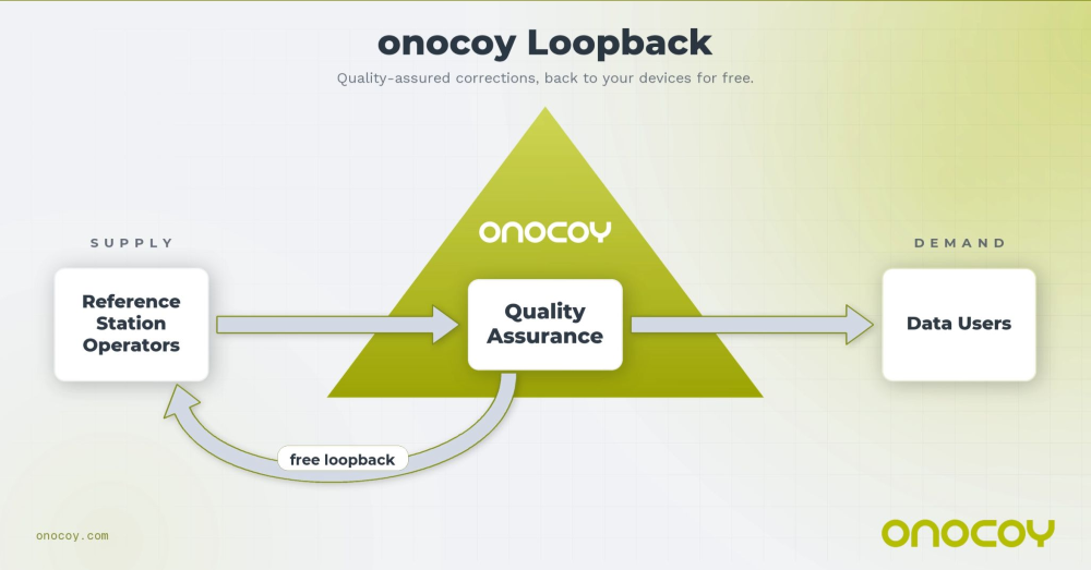
New feature eliminates the need for a self-hosted NTRIP caster and delivers enterprise-grade correction data to up to three devices simultaneously at no additional cost to the operator
Onocoy, a decentralized GNSS reference station network, is launching Loop Back, a new platform feature that routes quality-assured RTK correction data back to each station operator’s own devices free of charge. More than 7,800 active reference stations contribute to the onocoy network.
Operators who also needed precision positioning for their own drones, survey rovers, precision agriculture equipment, or autonomous machinery face a common friction point: the reference station they owned and operated produces valuable correction data, but routing that data back to their own field equipment requires either a separately maintained NTRIP caster or an additional subscription. Loop Back eliminates both.
Loop Back is immediately available to all onocoy station operators as a standard platform feature. Full documentation and setup guides are available at docs.onocoy.com.
How Loop Back works
When a GNSS reference station is connected to onocoy, raw observation data flows from the operator’s hardware into onocoy’s quality validation pipeline. The platform continuously checks position stability, multi-constellation health (GPS, GLONASS, Galileo, BeiDou), uptime and other parameters before producing a quality-assured RTCM 3 correction stream.
That validated stream has two destinations simultaneously: enterprise data clients who purchase GNSS reference station data through onocoy’s pay-per-use model, and the station operator’s own devices via Loop Back. The operator receives the same production-grade correction stream used by commercial clients, free of charge and with no data credits consumed.
Key capabilities at launch:
Up to three simultaneous active connections from an operator’s own devices to their own station’s corrections, with unlimited devices configurable
Compatible with any NTRIP-capable station regardless of hardware brand or model
Quality monitoring identical to that applied to enterprise client streams
No separate NTRIP caster required; onocoy manages the infrastructure
Free of charge: No data credits consumed for the operator’s own station data.
Who benefits
Loop Back is designed for the growing segment of professionals who both operate a reference station and rely on precision positioning in their daily work. Target use cases include:
Precision agriculture: Farmers running auto-steered machinery, UAV-based crop monitoring, and variable-rate application systems
Geomatics and surveying: Professionals running a base station and multiple rover units across a site, eliminating the overhead of a local base-rover setup
Autonomous systems, robotics and drones: Operators deploying multiple vehicles or aircraft requiring cm-accurate positioning for mapping, inspection, or delivery workflows
Research: Academic and scientific teams running parallel measurement campaigns from a shared base station.
Economics of station operation
Most professionals who deploy a GNSS reference station do so because their business in precision agriculture, surveying, drone operations and construction demands one. By connecting that station to onocoy, operators put the same hardware to work a second time: contributing data to onocoy’s global network and earning rewards worth several hundreds of U.S. dollars per year.
That additional income is enough to amortize the station in under two years before accounting for potential savings on subscriptions. Because onocoy applies continuous quality monitoring to every stream, operators also safeguard the positioning accuracy their business depends on.
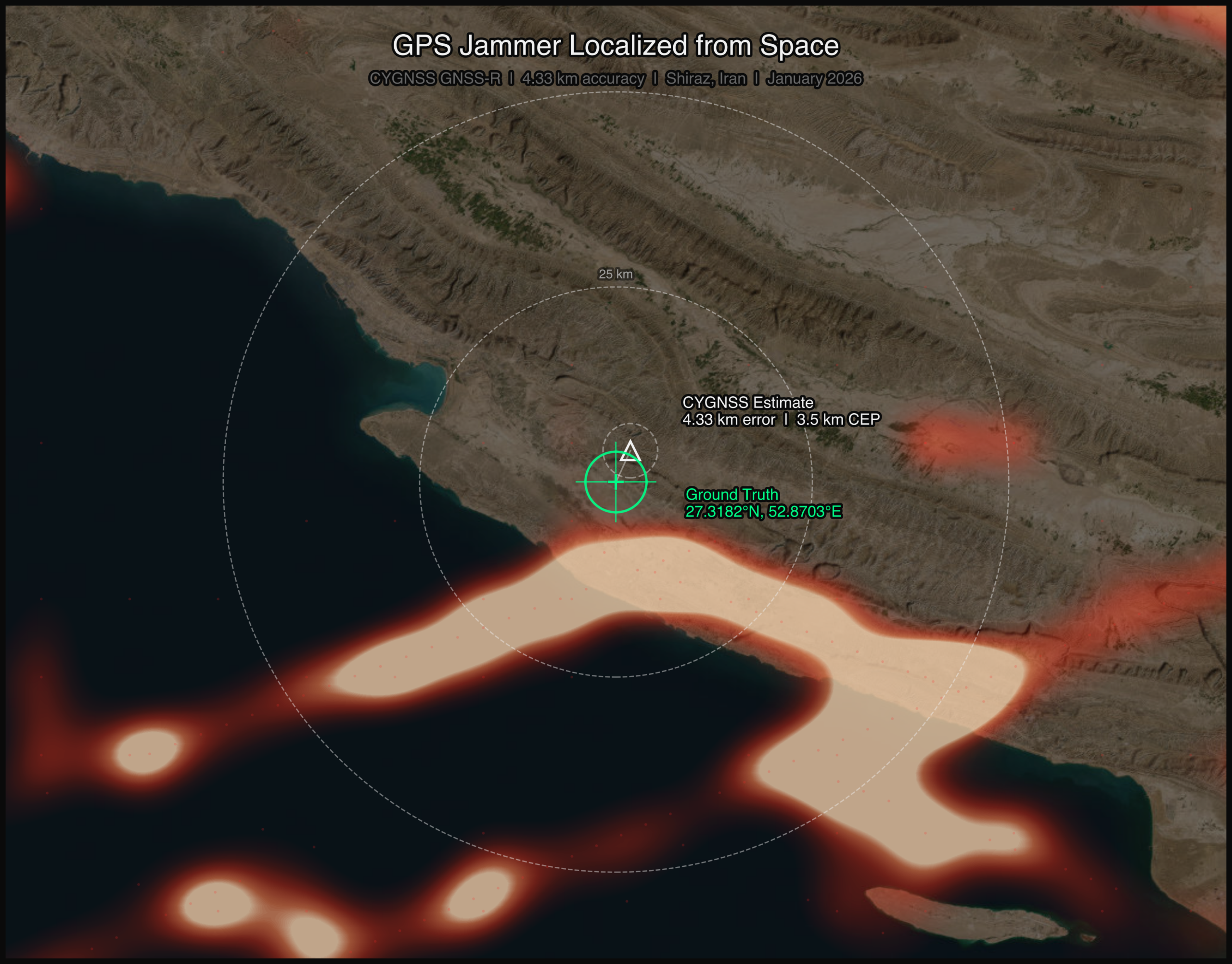
On a January morning in 2026, a GPS jammer powered up near Shiraz, Iran. It was not the first, and it would not be the last. The Strait of Hormuz corridor has become one of the most persistently jammed airspaces on Earth. But this time, two satellites were watching from very different vantage points, and together they would demonstrate something new: that spaceborne sensors can localize a terrestrial GPS jammer to within a few kilometers, using physics alone.
This article presents the first direct comparison of Cyclone Global Navigation Satellite System (CYGNSS) — a NASA GNSS reflectometry constellation — and NASA-ISRO Synthetic Aperture Radar (NISAR) — an L-band synthetic aperture radar for GPS jammer localization. The results challenge assumptions about which modality performs better and reveal that the answer depends on a question most analysts forget to ask.
The setup: Known jammer, known position
Validation requires ground truth. With help from the PNT community, we identified a GPS jammer operating near 27.32°N, 52.87°E (approximately 50 km southwest of Shiraz) that was active on Jan. 8 and Jan. 20, 2026, with confirmed quiet periods on Dec. 15 and Dec. 27, 2025. The jammer’s position was established through independent signals intelligence.
This gave us a controlled experiment: two “jammer ON” dates and two “jammer OFF” baseline dates, with satellite coverage from both CYGNSS and NISAR spanning the full period.
Two satellites, two physics
CYGNSS is a constellation of eight microsatellites that measure GPS signals reflected off Earth’s surface. Each spacecraft carries a delay-Doppler receiver that maps reflected signal power across a grid of delay and Doppler bins, known as the delay-Doppler map, or DDM. When a terrestrial jammer is active, it floods the GPS band with noise, elevating the DDM noise floor and suppressing the coherent surface reflection. The effect is detectable hundreds of kilometers from the jammer, creating a wide-area footprint in the reflected signal data.
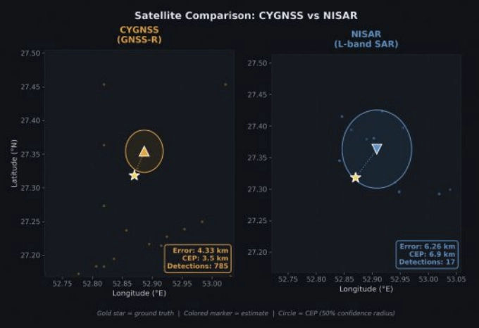
FIGURE 1 Jammer localization tracks from both CYGNSS and NISAR satellite constellations. (All figures by Sean Gorman)
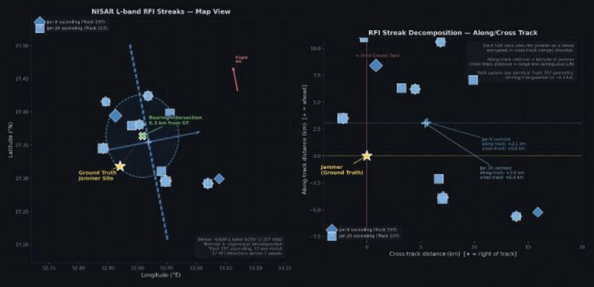
NISAR operates an L-band SAR at 1.257 GHz, just 30 MHz from the GPS L2 frequency at 1.2276 GHz. When a GPS jammer’s broadband emissions leak into NISAR’s receive band, they create characteristic streaks in the SAR imagery. The streaks are elongated in the cross-track (range) direction, not along-track, a counterintuitive result that follows directly from SAR signal processing. In azimuth (along-track), the jammer is a fixed-point source with a valid Doppler history, so the SAR azimuth processor focuses it correctly, similar to any ground target. But in range (cross-track), the jammer’s broadband noise does not match the SAR’s chirp waveform, so range compression smears the energy across many range bins rather than compressing to a point. The result is a streak perpendicular to the flight direction, whose along-track centroid encodes the jammer’s latitude and whose cross-track extent encodes a range arc, which is the distance from the orbit ground track (FIGURE 1). The bearing of each streak encodes the jammer’s direction relative to the satellite’s ground track.
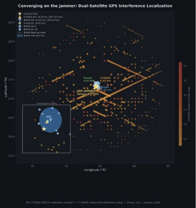
FIGURE 2 Crosstrack visualization for NISAR RFI streaks.
The two sensors could hardly be more different. CYGNSS sees the jammer’s effect on reflected GPS signals, offering an indirect measurement spread across hundreds of specular reflection points. NISAR sees the jammer’s emissions directly in its own receiver, which is a more precise measurement, but only along the satellite’s narrow ground track. FIGURE 2 shows both detection sets converging on the jammer location.
CYGNSS: 785 Detections, 4.33 km Error
We processed all CYGNSS Level 1 data within 200 km of the jammer location on both ON and OFF dates. Four detection methods contributed observations:
■ DDM noise floor (419 detections): The pre-computed ddm_noise_floor variable, calibrated against the thermal noise reference, proved the strongest discriminator. Near-jammer values exceeded 15,000 counts against a ~10,000 mean background.
■ Spatial noise grid (299):A 10 km gridded analysis identified cells with anomalously elevated noise relative to adjacent cells.
■ SNR hole detection (66): Coherent surface reflections were suppressed near the jammer, creating spatial “holes” in the SNR field.
■ NBRCS drop (1): Surface reflectivity dropped approximately 16% near the jammer, though this method produced few threshold exceedances.
Across four DDM channels per spacecraft and multiple passes, this yielded 785 total anomalous observations on the jammer-ON dates.
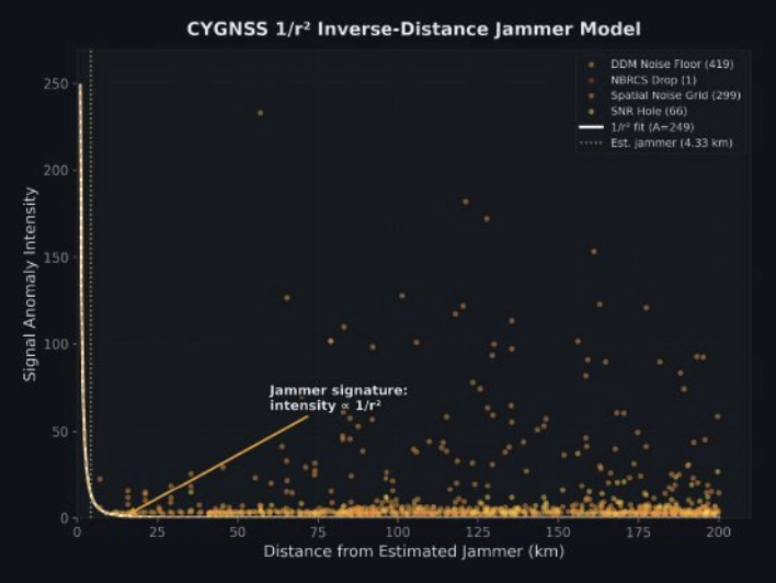
FIGURE 3 Scatterplot of interference insensity versus distance for CYGNSS.
Localizing using a simple centroid of all 785 detection positions placed the jammer 32.1 km from truth, with too many distant, low-SNR detections diluting the estimate.
Instead, we fit a parametric 1/r² inverse-distance model:
I(r)=Ar2
where A is a free amplitude parameter and r is the distance from a candidate jammer position. We jointly optimized the jammer position and amplitude using SciPy’s Nelder-Mead optimizer across all 785 observations, weighted by intensity. The optimizer converged on a position 4.33 km from ground truth, providing a 27.7 km improvement over the centroid (FIGURE 3).
The baseline: Zero false positives
On the jammer-OFF dates (Dec. 15 and Dec. 27, 2025), the pipeline produced exactly zero detections using the same thresholds, geographic area and satellites: a completely clean result. This suggests that the 785 detections are unlikely to be sensor artifacts or geographic anomalies. They disappear when the jammer turns off.
NISAR: 17 Detections, 6.26 km Error
NISAR’s approach is fundamentally different. Rather than measuring hundreds of reflected signals across a wide area, it captures direct emissions in a narrow swath, but with far greater geometric precision.
We processed NISAR L2 GCOV (geocoded covariance) products from Track 157, Frame 15 (ascending) for three dates: the Dec. 27 baseline and the Jan. 8 and Jan. 20 jammer-ON passes. The detection pipeline used eigenvalue decomposition of the polarimetric covariance matrix:
λ₁ ratio thresholding: In jammer-contaminated pixels, the dominant eigenvalue λ₁ of the 2×2 [HH, HV] covariance matrix rises sharply relative to the scene mean, indicating an unpolarized additive source.
Cross-polarization ratio (HV/HH): GPS jammer emissions are unpolarized, disproportionately elevating the HV channel. Anomalous HV/HH ratios flag contaminated azimuth lines.
Iterative outlier trimming: Three rounds of 1.5σ clipping removed scattered false detections, leaving 17 high-confidence streak centroids.
FIGURE 4 Error and CEP Metrics Comparison for CYGNSS and NISAR.
With detections from two passes on different dates, we had two independent bearing lines. Each pass’s streak centroids defined an azimuth aligned cluster whose major axis pointed toward the jammer. A PCA fit to the two clusters extracted the bearing: 308.1° from the Jan. 8 pass and 316.2° from Jan. 20. Their intersection — computed via scipy optimization of the angular residual — landed 6.26 km from ground truth (FIGURE 4).
The along-track/cross-track decomposition reveals why the 6.26 km error is a geometric ceiling for this dataset, not a processing limitation. Both passes come from the same Track 157 ascending orbit on a 12-day repeat cycle. The intensity-weighted along-track centroids land at +3.0 km and +3.1 km north of the jammer, a direct stable latitude measurement. The cross-track centroids land at +5.4 km and +5.6 km east of the orbit ground track, a range measurement. But because both passes share identical orbit geometry, the two range arcs are nearly parallel. The bearing difference between passes (308.1° vs 316.2°) is only 8.1°, producing a shallow intersection angle and poor cross-range resolution. A single descending pass, which would cross the ascending track at approximately 60-70°, would transform the geometry from two near-parallel lines to a genuine triangulation, potentially reducing the localization error to sub-2 km. Unfortunately, no descending NISAR pass covering this jammer site was available in the beta archive, which ends on Jan. 20, 2026.
The CEP (circular error probable, the radius containing 50% of repeated estimates) was 6.88 km, meaning if we ran this analysis on many similar jammers, half our estimates would fall within ~7 km.
Who wins?
CYGNSS wins, and not just on accuracy.
A naive confidence metric for the 1/r² fit would be the scatter of the 785 input detections (CEP = 127 km). But the detections are not the estimate; they are the inputs to a model fit. The relevant confidence question is: How stable is the fitted position?
We answered this with a 500-iteration bootstrap: resample the 785 detections with replacement, re-run the 1/r² optimizer each time and measure the spread of the resulting position estimates. The bootstrap CEP, the median radial distance across 500 fitted positions, was 3.48 km. The optimizer converges stably to within a few kilometers of the same location regardless of which detections are included.
This means CYGNSS achieves 4.33 km error with 3.48 km confidence, both better than NISAR’s 6.26 km error and 6.88 km confidence.
The bootstrap CEP also reveals what the raw scatter obscures: the 1/r² fit is constrained primarily by the ~80 high-intensity detections within 30 km of the jammer. The remaining 700 distant, low-intensity detections contribute little to the position estimate — they are correctly downweighted by the intensity-weighted least squares. The fit’s stability comes from the physics: a 1/r² signal has steep gradients near the source, providing strong positional constraints where it matters most.
Bayesian fusion: Can we get both?
The obvious next question: Can we combine CYGNSS’s wide-area sensitivity with NISAR’s geometric precision? We implemented four fusion strategies, all designed to work without ground truth:
■ Bayesian Gaussian posterior: Model each sensor’s estimate as a 2D isotropic Gaussian with σ = CEP/1.1774. The posterior is the product of the two Gaussians: an analytical precision-weighted mean.
■ NISAR-prior constrained 1/r²: Re-run the CYGNSS optimizer with a Gaussian regularization term pulling toward the NISAR estimate, sweeping the regularization weight λ from 0.01 to 10.
■ NISAR-proximity re-weighted 1/r²: Apply a Gaussian kernel centered on the NISAR estimate to the CYGNSS detections before fitting, effectively upweighting observations consistent with the SAR result.
■ Joint CEP-balanced: Combine the CYGNSS gradient signal with NISAR cluster proximity, weighted by (σ_CYGNSS/σ_NISAR)².
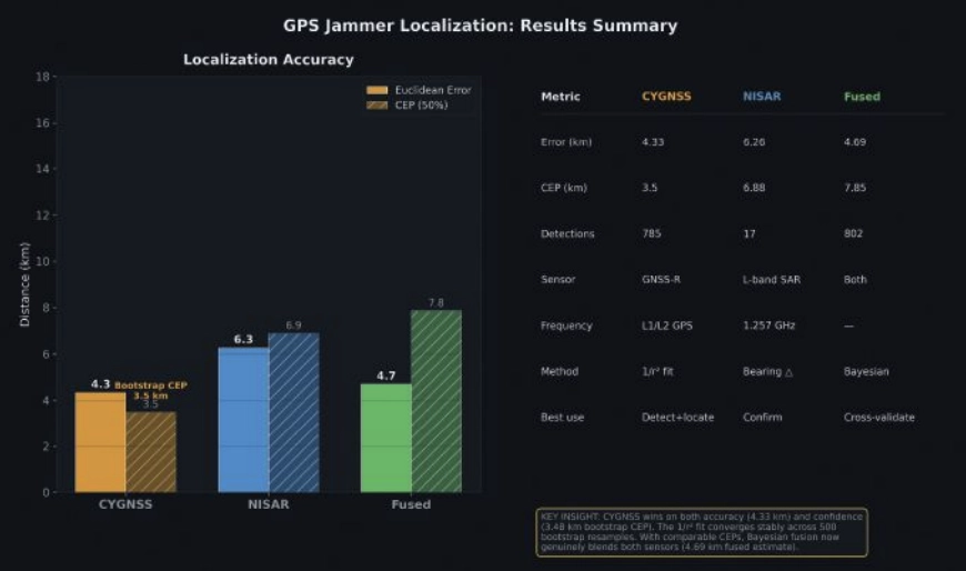
FIGURE 5 Summary statistics for jammer localization with CYGNSS, NISAR and fused approach.
With the bootstrap CEP, the precision ratio flips. The CYGNSS Gaussian (σ = 2.95 km) is now 2× tighter than NISAR (σ = 5.84 km). The Bayesian posterior, the precision-weighted mean, lands at 4.69 km, pulling toward CYGNSS’s better estimate while incorporating NISAR’s independent geometric constraint. FIGURE 5 shows the fusion: two comparable Gaussians whose product is tighter than either alone.
The fused result (4.69 km error, 7.85 km CEP) is not quite as accurate as CYGNSS alone (4.33 km), because NISAR’s 6.26 km estimate pulls it slightly away from truth. But operationally, the fusion provides a cross-validated answer: two independent physics arriving at similar locations builds confidence that neither sensor is producing an artifact.
The key insight is that the bootstrap CEP unlocked meaningful fusion. When the raw scatter CEP (127 km) was used, NISAR dominated the posterior 343:1 and fusion added nothing. With the fit-based CEP (3.48 km), both sensors contribute, and the posterior reflects genuine multi-modal evidence.
Operational implications
For CYGNSS: CYGNSS excels at both detection and localization. Its 785 detections across a 200 km radius, with zero false positives on baseline dates, provide unambiguous jammer detection. The 1/r² fit achieves 4.33 km accuracy with a bootstrap-verified 3.48 km CEP, meaning an analyst can trust the result to single-digit kilometer precision without ground truth. CYGNSS’s eight-satellite constellation also provides sub-daily revisit, enabling near-real-time monitoring.
For NISAR: NISAR provides independent geometric confirmation. With just two passes over an active jammer, the bearing intersection achieved 6.26 km accuracy with a 6.88 km CEP. The 6.26 km result is constrained by orbit geometry, not by detection sensitivity. Our two ascending passes from Track 157 produced nearly parallel range arcs with only 8.1° of bearing separation. Adding a single descending pass would provide a crossing angle of 60° to 70° and could reduce localization error to sub-2 km — transforming NISAR from a confirming sensor into a precision localization tool in its own right. The limitation in this study was data availability: The NISAR beta archive contained only ascending Track 157 passes over the jammer site. NISAR’s 12-day repeat cycle and fixed ground track also mean the jammer must be active when the satellite passes overhead. NISAR’s current value is as a confirming sensor — when both modalities converge on the same location, confidence increases beyond what either achieves alone.
For Fusion: With comparable CEPs (3.48 km vs 6.88 km), fusion now produces genuinely blended estimates. The Bayesian posterior at 4.69 km reflects real multi-sensor information. Future improvements, such as more NISAR passes with diverse bearings or CYGNSS multi-week accumulation, would tighten both estimates further.
For the Adversary: These results demonstrate that GPS jammers operating in contested airspace are observable and localizable from orbit using openly available civilian satellite data. The 4.33 km CYGNSS result is approximately 2× better than the published state of the art for GNSS-R jammer localization (~9 km grid resolution, Chew et al., 2023) and the NISAR bearing intersection approach has not been previously demonstrated for jammer geolocation.
Still broadcasting: Jammer persistence through conflict
The validation analysis used January 2026 data. But on Feb. 28, armed conflict erupted in the region. Did the jammer survive?
We ran the CYGNSS noise floor detection pipeline for each day from Feb. 28 through April 6, comparing against the December 2025 baseline. The answer is unambiguous: The jammer is not only still active — it is operating at dramatically higher power.
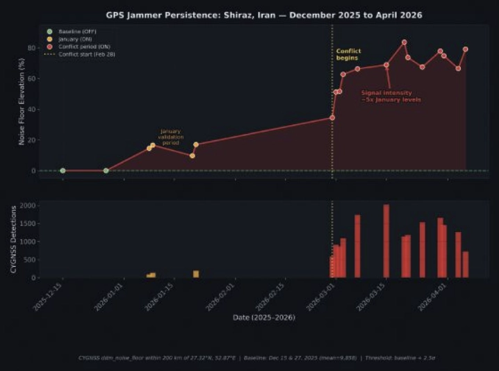
FIGURE 6 A timeline of jammer activity for Shiraz, Iran, from December 2025 to April 2026.
In January, the jammer elevated the CYGNSS noise floor by approximately 15% above baseline. By early March, days after the conflict began, noise elevation had jumped to 50% to 60%. By mid-March, it reached 70% to 84%, where it remained through early April. Detection counts tell the same story: 89 to 192 per day in January, rising to 1,000 to 2,000 per day during the conflict (FIGURE 6).
The escalation was immediate. On Feb. 28, noise elevation was +34.5%, already double the January level. By March 3, it had reached +62.7%, and by April 6, it peaked at +79.1%. The signal has remained at 5× the January intensity through the most recent available data (April 6, 2026).
Several interpretations are consistent with this pattern:
■ Power increase: The operator increased jammer output power, perhaps in response to the conflict or as a defensive posture against GPS-guided munitions.
■ Additional jammers: Multiple units may have been co-located or deployed nearby, creating an aggregate signature larger than any single device.
■ Duty cycle change: The jammer may have shifted from intermittent to continuous operation.
What is clear is that the jammer we localized in January was not incapacitated by the conflict. It was amplified. CYGNSS’s sub-daily revisit capability makes this kind of persistent monitoring possible using entirely passive, civilian satellite data — no tasking, no cooperation with the target state and no risk to reconnaissance assets.
Context and prior work
CYGNSS-based RFI detection builds on work by Chew et al., 2023, who demonstrated grid-level jammer detection at approximately 9 km resolution using DDM noise floor anomalies. Our 1/r² parametric fit extends this from detection to localization, achieving sub-5 km accuracy by exploiting the physics of signal power decay.
At the other end of the precision spectrum, Murrian et al., 2021, demonstrated ~220 m jammer localization using ISS-mounted Doppler measurements of raw intermediate-frequency (IF) data. This approach achieves an order of magnitude better precision than our methods but requires specialized hardware and raw signal access not available on current operational satellites.
The NISAR bearing intersection approach demonstrated here is, to our knowledge, the first published use of L-band SAR RFI streaks for jammer triangulation. The key insight is that NISAR’s proximity to GPS L2 (just 30 MHz separation) makes it an unintentional but effective GPS interference sensor.
Summary
Two satellites, two physics, one jammer. CYGNSS sees the interference footprint across hundreds of kilometers and localizes the source through inverse-distance physics. NISAR sees the emissions directly in its SAR receiver and triangulates through bearing intersection. Both achieve sub-7 km accuracy independently; together, they cross-validate and build the confidence that operational use demands.
The jammer near Shiraz is still there — louder than ever. The satellites are still watching.
Chew, C., Shah, R., Zuffada, C., et al. (2023). “Demonstrating CYGNSS as a Tool for Detecting GNSS Interference on a Global Scale.” IEEE Journal of Selected Topics in Applied Earth Observations and Remote Sensing.
Murrian, M.J., Narula, L., Iannucci, P.A., et al. (2021). “GNSS Interference Monitoring from Low Earth Orbit.” Navigation: Journal of the Institute of Navigation, 68(1).
NASA JPL. (2024). “NISAR L-band SAR Technical Specifications.” NASA/ ISRO SAR Mission Documentation. Closas, P., Fernández-Prades, C. (2023). “GNSS Interference Detection and Mitigation: A Survey.” Signal Processing, 206.
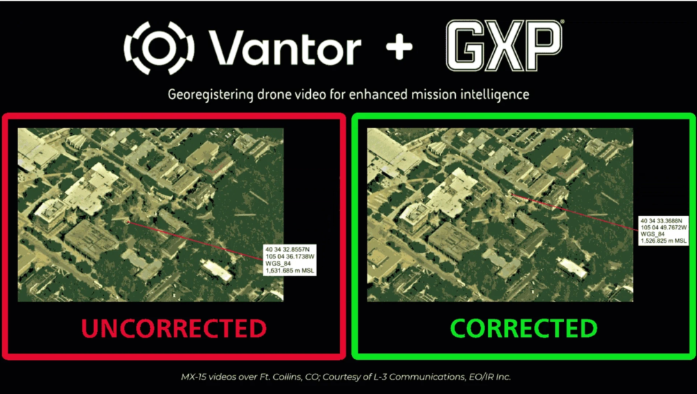
BAE Systems Geospatial eXploitation Products (GXP) and Vantor will be providing advanced intelligence and targeting capabilities for contested electronic warfare environments.
The delivery integrates part of Vantor’s Raptor, a vision-based software suite that enables autonomous systems to navigate, orient and extract accurate ground coordinates without relying on GNSS, with the GXP software ecosystem, ensuring intelligence continuity when sensors are degraded.
In modern conflict zones, the proliferation of inexpensive unmanned aerial systems (UAS) with equally low-quality sensors, in addition to widespread GPS spoofing and jamming, have rendered traditional drone video collection unreliable. Significant metadata drift in tactical video feeds leads to “targeting paralysis”: high-quality imagery is available, but the underlying geographic coordinates are too inaccurate for precision activities.
To solve this, Raptor Sync georegisters the full-motion video feed from the drone’s on-board camera with Vantor’s 3D terrain data in real time, enabling downstream GXP intelligence fusion, multi-domain interoperability across different sensors, and accurate ground coordinate extraction at a demonstrated absolute accuracy of <3 m. The system enables previously impossible intelligence and targeting workflows.
“In contested environments, the sensor’s imagery and video collections are only half the battle; the accuracy of the data it produces is what determines mission success,” said Kurt de Venecia, senior director of Product Development at BAE Systems GXP. “By including Raptor directly into our GXP intelligence workflows, we are providing analysts with the ability to maintain absolute targeting confidence, even when the platform’s systems or inertial sensors lack high absolute accuracy.”
Injecting corrected key-length-value (KLV) metadata from Raptor directly into the drone’s video stream at the edge enhances accuracy prior to exploitation in GXP software. This overrides inaccurate telemetry, enabling analysts using GXP solutions to extract weapon-quality coordinates and execute intelligence and targeting missions in real time.
“Analysts cannot afford to lose confidence in where a target actually is,” said Paul Millhouse, senior director ofRaptor Products at Vantor. “By using Raptor to correct video before it enters the GXP Ecosystem, we’re enhancing the performance of existing and new drone fleets. The result is a more resilient workflow for extracting accurate ground coordinates and maintaining operational tempo.”
These capabilities will be highlighted at GXP360° Professional Exchange & Workshop in San Diego, California (May 18-20).
Telit Cinterion and Swift Navigation have announced an expanded partnership. Telit Cinterion will offer Swift Navigation’s Skylark Precise Positioning Service as part of an integrated IoT positioning solution.
This service is available with Telit Cinterion’s dual-frequency GNSS modules and NExT cellular connectivity. IoT customers gain one source for the hardware, connectivity and Skylark Dx correction data needed for sub-meter positioning.
What began in 2024 as a technical partnership has grown into a comprehensive joint offering, uniting hardware, connectivity, and corrections into a seamless solution for IoT customers.
Telit Cinterion customers can now buy modules, connectivity and corrections under one contract. For many IoT projects, this cuts vendor coordination and avoids the cost and operational complexity of building or subscribing to an RTK base-station network.
Skylark is available in three variants — Skylark Dx, Cx, and Nx RTK — to meet a broad range of requirements for accuracy, coverage, bandwidth, and power consumption.
All Telit Cinterion dual-frequency L1 + L5 GNSS modules offer native support for Skylark Dx, which streams differential GNSS (DGNSS) corrections directly to the receiver over the cellular network. Skylark Dx runs over standard RTCM via Internet Protocol (NTRIP), using minimal bandwidth and power, and provides country-wide coverage. This makes it practical for IoT devices with limited bandwidth or tight power budgets.
Typical applications include:
e-mobility
fleet and asset tracking
robotics
drones
These are cases that don’t require centimeter-level RTK accuracy but do need reliable sub-meter positioning. Customers requiring higher accuracy can upgrade to Skylark Nx RTK on compatible module variants without redesigning their devices or changing suppliers.
“Customers tell us they want precise positioning without complexity,” said Neset Yalcinkaya, president of IoT hardware at Telit Cinterion. “We’re bundling Skylark Dx with the GNSS modules and cellular connectivity we already ship. This gives customers one supplier and a single integration approach, plus a clear path to RTK down the road.”
“At Swift Navigation, our mission is to make precise positioning a standard capability,” said Holger Ippach, chief operating officer at Swift Navigation. “This partnership advances that vision by embedding Skylark into Telit Cinterion’s GNSS modules and connectivity, giving customers direct access to reliable, sub-meter positioning without the integration overhead traditionally required.”
Service Availability
Skylark Dx is available now with Telit Cinterion solutions in Europe, North America, Japan, South Korea and Taiwan. Coverage will expand as Swift Navigation adds regions.
Data provides baseline measurement for tracking change at one of Earth’s last tropical ice fields in Puncak Jaya, Papua, Indonesia.
Trimble is supporting Project Pressure by providing advanced GNSS positioning technology and research funding for the nonprofit organization’s latest expedition to map the disappearing tropical glaciers of Puncak Jaya in Papua, Indonesia.
Project Pressure has released a centimeter-accurate, 3D model of the receding ice, created using Trimble positioning technology and drone-based photogrammetry. The model establishes a scientific baseline for calculating the rate of glacier recession and projecting the timeline of disappearance.
Puncak Jaya, the highest peak in Oceania and one of the Seven Summits, is expected to be the first of the seven continental peaks to lose its glaciers as global temperatures rise.
Puncak Jaya has the only snow in Indonesia. (Credit: Enda Kaban, CC BY-SA 4.0)
Local communities use the data to make informed choices about crop selection and prepare for expected water shortages caused by the loss of vital reservoirs.
This expedition marks the third successful outing in Project Pressure’s “Melting Topics”series, which focuses on mapping equatorial glaciers. Trimble provides its GNSS mapping technology and research funding from the Trimble Foundation Fund to support Project Pressure in gathering critical data in some of the world’s most remote and hostile environments.
“Mapping these glaciers before they disappear is of critical importance to establish a baseline to track the glacial regression and for the local communities to understand what is happening with their water source, allowing them to adapt to a changing climate,” said Eliot Jones, senior manager, strategy and partner development at Trimble. “Through a combination of precision technology, detailed project planning and rigorous science, the models created by Project Pressure are shared for scientific study and provide a visual reference for future generations.”
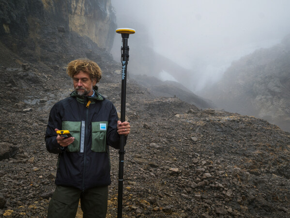
Precision under pressure in hostile terrain
Mapping glaciers at altitudes exceeding 4,800 meters (15,000 feet) presents extreme logistical and environmental challenges. Near-constant cloud cover and heavy rainfall in Papua often render satellite imagery unusable, making ground-based georeferencing essential.
The expedition team installed precise geolocation reference points directly on the glacial surface at multiple locations. Using the Trimble Catalyst DA2 GNSS system and Trimble TDC600 handheld, researchers captured the exact coordinates of those points with centimeter-level accuracy. Drone imagery was then processed against the Trimble coordinates to produce a scientifically reliable 3D model of the glacier.
“Trimble makes incredibly complex technology feel simple in the field,” said Klaus Thymann, scientist and lead explorer. “When you’re standing on a glacier in freezing conditions, wearing thick gloves and surrounded by clouds, you don’t have time to fight with equipment. With Trimble, I can capture centimeter-accurate readings and the interface is so intuitive that even someone with no prior training can help collect data. That kind of reliability and simplicity is critical when you’re working in some of the most remote and challenging environments in the world.”
This approach builds on methods developed during Project Pressure’s 2024 expedition to the Rwenzori Mountains in Uganda, which also used Trimble technology.
The lightweight Trimble Catalyst DA2 GNSS system was critical for the expedition, which required helicopter access to Basecamp, followed by a trek to the launch point.
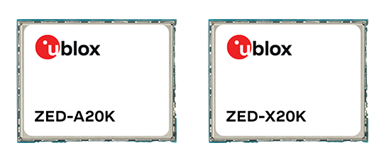
U-blox has expanded its automotive GNSS portfolio with the launch of two highly specialized modules: the ZED-X20K and the ZED-A20K. This dual release addresses engineering needs of both mass-market advanced driver assistance systems (ADAS) and safety-critical autonomous architectures.
Both modules feature pin-to-pin compatibility, enabling platform flexibility and simplifying product development across vehicle generations as well as jamming and spoofing detection to mitigate the impact of security risks.
The ZED-X20K is designed for mass-market ADAS L3 and TCU/IVI applications, delivering lane-level accuracy worldwide using all-band GNSS and native Galileo High Accuracy Service (HAS). By eliminating the need for paid correction services, backend infrastructure, or service management, it reduces total cost and accelerates time-to-market while maintaining consistent global performance.
For applications that require a functional-safety concept for GNSS sensors, the ZED-A20K introduces a new architectural approach. It provides ISO 26262 ASIL-B(D)-compliant GNSS RAW data simultaneously to high-performance QM positioning outputs within a single module. This enables OEMs to transition from traditional dual hardware based-GNSS systems to a single module approach, reducing system complexity and cost.
With flexible support of externally hosted positioning engines, especially for ADAS of Levels 3 and up, the A20 concept enables enhanced flexibility for SDV–based architectures. The form-factor compatibility between ZED-X20K and ZED-A20K allows the flexibility to equip different trim levels with or without functional safety requirements out of a single socket.
The ZED-X20K has reached the engineering sample stage, and its evaluation kit is available. Samples for the ZED-A20K will be available starting in August.
The new autopilot is engineered to provide reliable GNSS‑denied navigation and fully autonomous mission execution, including complex operational scenarios and seamless interoperability.
UAV Navigation — a division of Grupo Oesía specializing in advanced guidance, navigation and control solutions for unmanned vehicles — has launched the Vector-300high‑performance autopilot.
Vector-300 is designed to meet the industrial and operational requirements of mass‑produced, attritable unmanned aerial systems, with a clear focus on loitering munition and Counter-UAS (C-UAS) interceptor applications.
Vector‑300 has been engineered to combine advanced autonomous guidance, navigation and control (GNC) capabilities with scalability and manufacturability. Its architecture is designed to reduce technical complexity and enable agile, large‑scale production while ensuring consistent and reliable performance across high‑volume deployments.
Designed for high‑dynamic interception and terminal missions, Vector‑300 delivers strike‑to‑target precision guidance with bull’s eye accuracy. The autopilot supports the integration of AI‑based target identification and optical data directly into its autonomous GNC loops, enabling advanced engagement of both static and dynamic targets. This architecture supports real‑time trajectory adaptation during pursuit and terminal engagement phases, making Vector‑300 suitable for demanding loitering munition and C-UAS interceptor operations.
Vector‑300 is designed to operate in highly contested and GNSS‑denied environments, even under electronic warfare (EW) jamming, spoofing and meaconing. Its robust navigation core relies on advanced inertial algorithms and multisensor fusion to ensure mission continuity across all phases of operation and can be easily complemented with UAV Navigation–Grupo Oesía proprietary solutions such as the Visual Navigation System to enhance dead‑reckoning accuracy.
Building on the battlefield-proven capabilities of the Vectorautopilot family, Vector‑300 enables the full range of advanced operations already established across UAV Navigation–Grupo Oesía solutions. These include
fully autonomous mission execution
swarming and formation flight
4D trajectory management to reach targets at a predefined time
high‑dynamic maneuvers
manned‑unmanned teaming (MUT) operations
many other advanced autonomous capabilities.
Its open and modular architecture is designed to ensure interoperability with third‑party platforms, payloads and sensors through seamless integration with Vector‑MCC. This architecture also enables the integration of autonomous decision‑making software, allowing platforms equipped with Vector‑300 to adapt to evolving concepts of operation and advanced autonomy requirements.
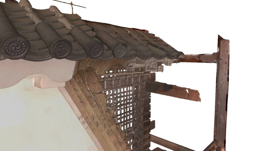
Using Artec Jet, Artec Ray II and Artec Leo, 3D scanning experts have digitized Japan’s historic Odawara Castle for heritage preservation and potential future restoration projects
Challenge: Capturing a massive heritage site, including every detail from courtyards and buildings down to a drawbridge and individual rivets on castle gates.
Solution: Artec Jet, Artec Ray II, Artec Leo, Artec Twins
Result: A single, interconnected point cloud covering the entire facility — scanned mostly with Artec Jet, but with areas of interest captured more accurately using Artec Ray II & Leo. The resulting high-density dataset can be explored in 3D, making it suitable for virtual museum tours, or continuous monitoring to ensure Japan’s famed Odawara Castle stands the test of time.
Why Artec 3D? The highly maneuverable Artec Jet can be attached to a backpack and simply walked through an environment. Entire scenes can be captured from ground level in minutes, including tall structures from a range of up to 300 meters. Artec Ray II and Leo deliver higher accuracy for applications like long-term monitoring, damage assessment, and restoration.
Odawara Castle: A gateway into Japan’s past
Odawara Castle was built more than 500 years ago, with fortifications first erected during the Kamakura period — a time famous for the emergence of the Samurai and Japan’s first Shogun.
The site’s illustrious walls are steeped in history. Situated on a hill and surrounded by a moat, the castle has strong fortifications, so it was coveted and fought over for generations. Three sieges of Odawara took place from 1561-90 and the structure changed hands (and shape) multiple times over the next century as different leaders left their stamp on the property.
At times, the legacy of Odawara Castle has been difficult to protect. The entire site was shaken to its foundations by multiple earthquakes from 1703-1853 and the Meiji government of the late 19th century ordered that all feudal structures be destroyed, so it was mostly torn down.
In 1938, what remained of Odawara Castle was made a heritage site and slowly rebuilt. But over the years, it has remained a delicate piece of history in need of ongoing renovation. With this in mind, the Artec 3D support team — in Japan for a recent trade mission — opted to digitize the entire structure for future generations to enjoy using Artec Jet, Artec Ray II and Artec Leo.
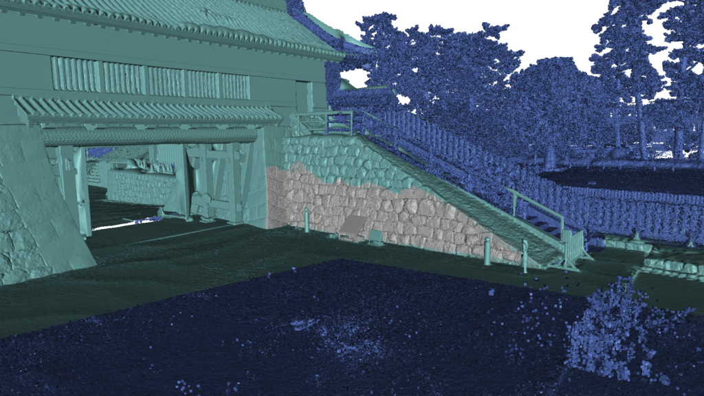
Artec Jet (dark blue), Artec Ray II (light blue), and Artec Leo (grey) point-cloud data fused together for high detail on every scale. (Credit: Artec 3D).
Capturing an entire castle in minutes
When they arrived at the castle, engineers immediately understood the scale of the challenge they were embarking on. Once one of medieval Japan’s largest fortifications, the site’s outer defensive perimeter is a whopping nine kilometers long. Odawara Castle is also a national landmark that’s open to visitors, so they didn’t have the facility all to themselves either.
This meant that speed and subtlety were critical. It would’ve been entirely possible to capture the site with a lidar, tripod-mounted Ray II, by positioning it around different areas of the fort. But this would take a prohibitive amount of time — especially when you consider that double scans are required to remove moving objects. Using Artec Jet was a lot more straightforward.
Attaching the device to a backpack meant the castle could be scanned on foot. Walking the site, almost as if they were a tourist, was enough to capture the entire scene. Artec Jet’s remote app gave real-time feedback on scan progress, so the team didn’t leave any detail uncaptured — and compared to capture with shorter-range scanners, the time savings were enormous.
“Artec Jet scans in a linear fashion. If it takes you two minutes to walk, it’ll take two minutes to scan — the complexity of the scene has little bearing,” explains Artec 3D scanning expert Keynan Tenenboim. “In the same time it took for Leo to scan 2-3 walls, Ray II scanned a building, and Jet digitized an entire castle. Adding in Ray II & Leo was great for areas with accessibility issues — and capturing higher detail around the walls, gate, and courtyard.”
A Trio of Scanners for the Task
Natural environments like trees, rivers, and larger connecting spaces often offer valuable site context, but don’t need to be captured with high accuracy. Artec Jet was perfect for picking up this sort of background information, generating a continuous point cloud, and connecting the site’s more interesting features: historic walls, ornate roofs, and courtyards around the castle.
Jet’s 300-meter range meant there was no need for ladders or scaffolding. The inner structure was captured from ground level without other visitors even noticing. Unlike Ray II, which scans from static viewpoints, Jet could also be maneuvered into difficult-to-reach areas. Both scanners are less accurate than Leo — but that’s why it’s best to combine datasets, for peak results.
In this case, Ray II was deployed to scan the inner courtyard and gate, with Leo being used to pick up smaller details like the confined area behind the entrance. Handheld 3D scanning was also perfect for capturing a nearby medieval wall. As you can see from the scan below, fine details like tile patterns, lettering, and the wall’s internals were all captured in a single sweep.
“This was the perfect project for demonstrating the benefits of all three scanners,” said Tenenboim. “The main castle wouldn’t be a good fit for Leo and it didn’t really fit Ray II. There was no good vantage point where we could see the facade from 100 meters away. Thanks to Jet’s range, we were able to scan from a ground level. Okay, we could’ve improved roof capture by flying Jet on a drone — but this would require more site preparation.”
Fine details of an exterior wall captured just outside the castle with Artec Leo. (Credit: Artec 3D)
Heritage preservation with end-use potential
Once engineers had finished scanning, they sent data back to Artec’s Luxembourg HQ via cloud sharing for processing in Artec Twins. Specifically designed to handle large datasets, Artec Twins software allows Artec Jet, Ray & Leo scans to be merged — either into a unified point cloud, or a 3D mesh that can be measured and exported to industry platforms like Autodesk Revit.
In terms of applications, the resulting 3D point cloud would be perfect for building a virtual museum tour that allows visitors to virtually explore Odawara Castle. Regular data capture sessions would also allow site operators to monitor conditions over time. If a building’s traditional rooftop began to sag, for example, it’d be possible to carry out rapid repairs.
Deployable in seven modes: by-hand, backpack, pole, cage, robot, vehicle, or drone, Artec Jet adapts to any environment, allowing users to replace complicated multi-tool workflows. Clearly, Artec’s Odawara Castle scan is just the beginning, there are many more sites left to explore.
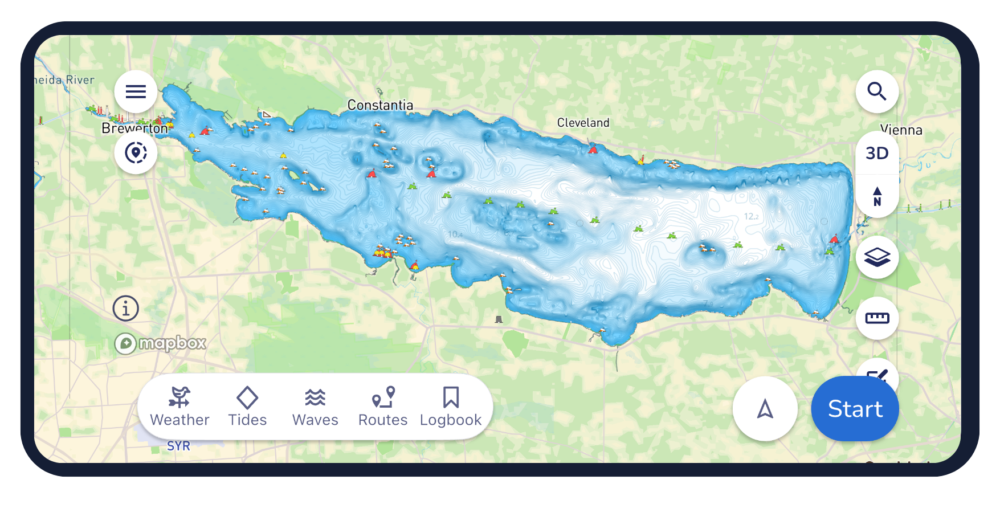
Marine navigation company Savvy Navvy has developed an in-house approach to processing and reconciling fragmented hydrographic data — combining official hydrographic data with expert geospatial data analysis to scale chart coverage faster and with greater accuracy.
The latest rollout adds more than 2,200 U.S. lakes and extends coverage into Estonia, Lithuania and Latvia in Europe, opening more waterways for boaters across the globe to explore. This comes not long after Danish charts from hydrographic offices were also added to the navigation app.
Prioritized by where boaters are most active, the latest update includes all major Minnesota lakes and expands lake coverage in 20 other U.S. states.
Elena Petru. (Credit: Savvy Navvy)
“Land mapping across much of the developed world, has benefited from sustained investment over several decades. Hydrographic data, the mapping of water, has a different history,” explained Elena Petru, geospatial data engineer at Savvy Navvy. “Survey cycles are longer, coverage is uneven, and for inland waters like lakes and reservoirs the situation is patchier still.
“Multiple authorities may hold overlapping or conflicting data for the same body of water, formats vary, and there is no single canonical source that can simply be downloaded and trusted. This fragmentation is exactly the challenge our geospatial team is solving through a structured reconciliation process.”
Petru joined Savvy Navvy in 2023, bringing her geomatics background from land data roles into the specific challenges of marine and inland water charting. Her expertise has enabled development of new data pipelines to overcome these marine charting challenges — marking a significant step in Savvy Navvy’s ongoing chart development program being based on unique, comprehensive data.
“You’d be surprised how often official sources do not fully line up. One of the main challenges is that the same lake can be represented slightly differently depending on the dataset. The task was not to pick one and apply it, but to compare sources carefully, understand where they differed, and make informed decisions about how each lake should be represented,” Petru said. “By going beyond official sources with our own expert validation process, we can integrate new regions faster while maintaining high data integrity, which overcomes one of the biggest difficulties in marine navigation. It’s exciting to see this data go live in the Savvy Navvy app knowing boaters can now use it on the water every day.
This approach forms part of Savvy Navvy’s broader data processing pipeline, enabling consistent, repeatable expansion into new regions. Through these data pipelines we can now deliver faster, more expansive chart coverage including waters not yet fully covered by official hydrographic surveys.
Savvy Navvy has been downloaded more than three million times globally. Unlike other boating navigation solutions, Savvy Navvy provides smart routing, giving users optimal routes and dynamic ETAs based on real-time data: departure time, chart information, weather conditions, tide, boat specifications and local regulations. The updated chart coverage is available across both the Savvy Navvy app and its integrated solutions.
Last month Savvy Navvy launched its new waves feature, turning complex wave data into a simple visual view that helps boaters understand how conditions will actually feel on the water. Worldwide chart coverage is available on all Savvy Navvy plans.
Without hesitation, the family awakened from their sleep, grabbed wallets, smartphones, car keys and hurriedly descended the stairs into the shelter. Doors sealed, the children crawled into their shelter beds.
The mother and father, listening to the weather radio, heard their county’s name in the emergency broadcast. They looked at the smartphone’s weather map blinking with the text alert. A large swath of rain covered the area, painting yellows and reds inside a field of green. At the trailing edge of the storm, where skies were beginning to clear, the storm’s red tail began curling into a ball, moving directly toward them. Inside the ball, a dark red deepened into a growing magenta core. White pixels appeared within the magenta tail. Its path was unchanged and it was closing.
The man and woman huddled together watching the storm radar app on his mobile device not thinking about how their situational awareness is a confluence of spatial wizardry and atmospheric thermodynamics. The WSR-88D NEXRAD (Level III) radar scans a 143-mile radius, sweeping 14 elevation angles every five minutes to create a composite view of the surrounding weather. Colors correspond to the intensity of reflected hydrometeors (forms of precipitation) ranging from 0 dBZ, light rain in blue and green, to 75 dBZ, hail in magenta, and at 95 dBZ, it is physical debris carried aloft showing as white. Assembling the radars from across the country creates a seamless national weather mosaic (weather.gov/Radar). The dot on the smartphone’s weather app marking their own position is GNSS, orbiting far above.
In his hand both the NEXRAD and GNSS are blended in real-time as he watches the Tornado Vortex Signature (TVS) move toward his family and his house. Beyond the closed shelter doors, tornado sirens wail, mixed with peals of thunder. The warnings are no longer county names but names of towns. There are people for whom such a moment is not hypothetical. Scott Bagenzie knows exactly what comes next, not from imagination but from experience.
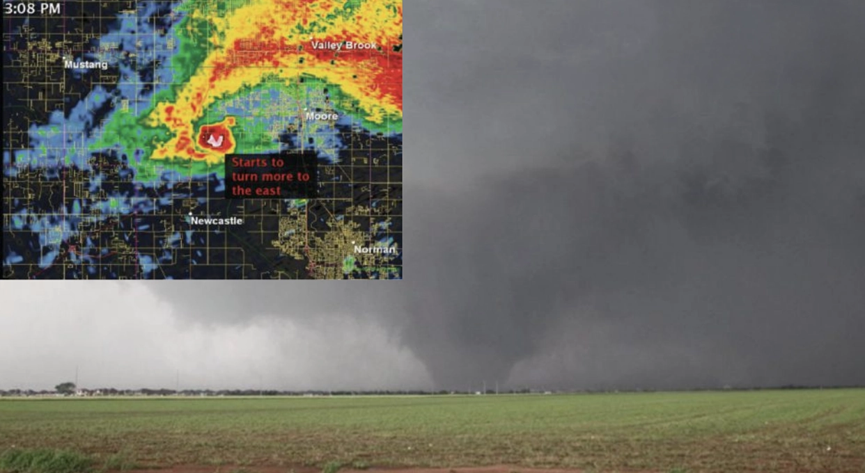
On Monday, May 20, 2013, at 2:56 p.m. Central Time, an EF5 tornado touched down northwest of Newcastle, Oklahoma, rapidly intensifying as it carved a path to Moore. The tornado lasted 36 minutes and covered 17 miles (FIGURE 1). Scott was caught by it, and I had the privilege of hearing him tell me what it is actually like to be inside those moments of sheer terror the rest of us only read about. He left work at 2:15 p.m. despite National Weather Service warnings for the counties flanking Oklahoma City. As he closed his car door, the sirens at the Mike Monroney Aeronautical Center went off. Security tried stopping him. He drove anyway.
“I was dodging cars left and right as people were taking pictures out to the southwest. I called Mari and said, hey, I’m running to the house to make sure the pets are taken care of. And she said, You crazy ***, take care of yourself.”
He pulled into his driveway, secured two cats in the closet and the dogs in the front bathroom, then stepped outside to see where the tornado was. His neighbor, who had an underground shelter in his garage, called out from next door: Get in over here! Scott went. As soon as the latch clicked behind them, debris began hitting the house above.
Weather as GIS
Weather is the most common topic of greetings. It is often the front page on newspapers. Television news is incomplete without a weather report, and weather is among the most downloaded apps on smartphones.
In many ways, the first GIS was weather, starting in the mid-1800s, long before computers, GNSS and GPS, hand-plotting data points, and then hand-drawing lines of equal pressure, temperature, humidity and winds on charts.
In the 1990s as a U.S. Navy weather specialist, I drew these charts by hand, plus four upper air charts learning how 3D spatial volumes interact. That was manual GIS. Now, in 2026, weather continues leading geospatial innovation via phased array radars, dual-pole radars (horizontal and vertical scans), acoustic atmospheric sensors, and predictive modeling for weather and climate, all of them layering atmospheric data using complex algorithms to forecast a dynamic fluid medium moving over an irregular spinning sphere that is unevenly heated. It is remarkably accurate, pushing the edges of geospatial predictive modeling.
The architecture of violence
The primary driver of powerful tornadoes is atmospheric thermodynamics unique to North America. Dry air crossing over the Rockies, cold arctic air pulled south by the jet stream, and warm moist air drawn north from the Gulf of America converge in a cauldron that can boil a normal convective storm into a sustained mesoscale supercell producing EF-5 tornadoes, the most powerful on record. Even though they make up less than one percent of all tornadoes, it is rare for EF5 tornados to occur anywhere else on Earth.
The Enhanced Fujita (EF) scale for measuring them was developed in 1971 by Theodore Fujita, a Japanese engineer whose forensic study of atomic bomb blast damage at Nagasaki and Hiroshima led to his damage-based framework for measuring tornado intensity.
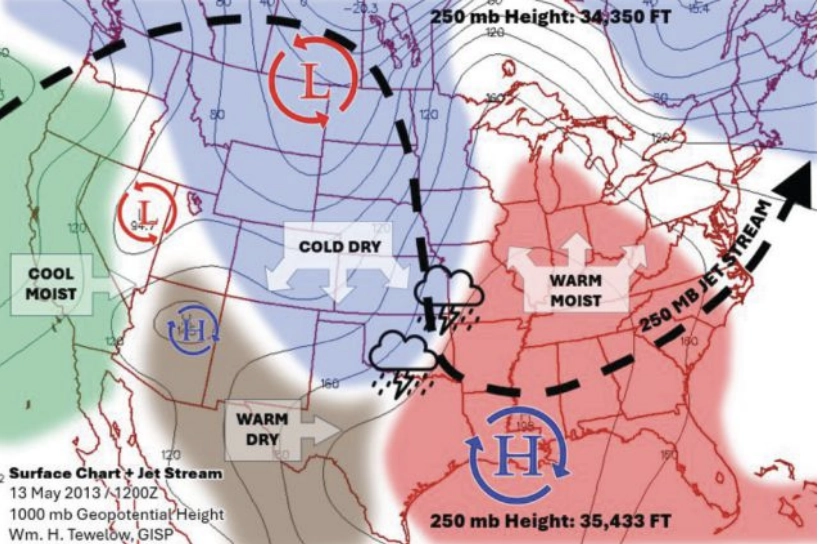
FIGURE 2 This NOAA chart shows a height of 250 millibars (mb) of pressure over Tornado Alley in the U.S. (Credit: William Tewelow | Chart from NOAA NWS)
The jet stream, a river of air riding a thermal pressure gradient in the upper atmosphere, creates vorticity as cold dense arctic air plummets south, wedging beneath the warmer Gulf air and forcing it upward along the frontal boundary, before the jet stream curves back north. FIGURE 2, the 300 mb (mb stands for millibars of pressure) chart, shows this process has caused a low pressure over Texas sitting in a 1,200-foot-deep ravine. A jet streak will form as air rushes into the ravine increasing the jet stream’s speed, which draws in rising convection currents that can spawn mesoscale storm cells and set up the potential genesis of severe tornadoes.
When a funnel cloud forms, it is the visible physics of pressure dropping the temperature to the dew point causing condensation. The dropping pressure forms a bowl shape. Air flows into the dropping pressure, and the base of the cloud rotates cyclonically. As the rotation increases, centrifugal force of the colder dense rotating air pushes out the warmer higher-pressure air, further lowering the pressure at the core and deepening the bowl. That continues as the base descends into higher pressures at the surface, tightening the bowl into a cone. The difference in pressure between air outside the cone and what’s inside the vortex core can be 100 mb. That is basically a hole and wind rushes in to fill that void, but centrifugal force acts against the air. A tornado is born.
Wraiths of destruction
On May 31, 2013, 11 days after Moore, a multiple-vortex tornado formed near El Reno, Oklahoma. Along its periphery, small vortices spun around the rotating edge, circling, combining, breaking apart, vanishing and reforming, like wraiths of destruction dancing in a ring. The column darkened, descended and enveloped its own micro-vortices, forming the largest tornado ever recorded: 2.6 miles wide at its base.
It grew so rapidly that experienced TWISTEX storm chasers attempting to place instrument disks behind it were consumed as it expanded from 1.6 miles to 2.6 miles wide. A father, his son, and a colleague were killed; their car was found eight miles away.
Storm chasers are not thrill-seekers. WSR-88D NEXRAD, even at its lowest scan angle, already sits at 14,000 ft at its range limit because of the Earth’s curvature; spotters provide the ground truth radar cannot. Instruments such as Ground-based Local Infrasound Data Acquisition (GLINDA) extend that capability further: Tornadoes produce infrasound as low as 0.5 Hz, with a correlation between tornado size and frequency that may one day provide an early warning radar cannot.
I asked Scott whether he felt the tornado before he heard it.
“I couldn’t feel it,” he said, “but I could hear the sound of the train coming.”
I pressed him to describe it beyond the cliché. He thought for a moment, then said, “It’s not a cliché. That is what it sounds like. It sounds like a freight train, and the sound of the house being torn apart.”
The roar grows
Back in the shelter, the physics unfolded exactly as Scott described. Unaware of the sensation, a deep groaning sound resonates miles ahead of the tornado. A low constant roar grows louder as it approaches. Explosions pop as transformers blow. The shelter is pitch black except for the phone screen, that small glowing window showing a white ball of catastrophe moving toward them. The roar grows louder. Ears pop. Temperature drops. The house shakes. The roar of the freight train is so loud the screams inside the shelter cannot be heard. The doors rattle. The whirlwind is trying to break in. Then the roar fades, almost to silence, an eerie quiet.
In Scott’s shelter, the sequence was identical. His ears popped suddenly and painfully; they hurt for a full day afterward. In an EF5 tornado, pressure drops from roughly 950 mb in the surrounding air to 850 mb at the vortex core. The 100 mb passing over him was equal to a 3,000-ft pressure drop. It is the equivalent of instantly ascending two Empire State buildings stacked on top of each other, like falling straight up into the sky. Fighting against that force, Scott and his neighbor held shut the shelter latch as the doors bounced on their hinges.
“I don’t know how well those are constructed. I didn’t take any chances.”
Nearby, employees sheltering in a bank vault were physically holding the vault door closed as the tornado passed a thousand feet away. The vault’s timed lock could not engage. Five or six people leaned against a door designed to stop a robbery, fighting powerful thermodynamic forces.
Then Scott no longer had to hold the latch. The truck on the other side of the garage wall had been pushed against the hatch from outside, pinning them in. When they finally forced it open and stepped out. There was nothing.
“She just started screaming. She said, ‘No way, it didn’t do that.’ I told her, yeah, there’s nothing left.”
The entire event, from first debris strike to silence, lasted roughly one minute. At 28 miles per hour, a tornado traverses one mile in two minutes, plowing through a neighborhood in seconds.
Mapping the aftermath
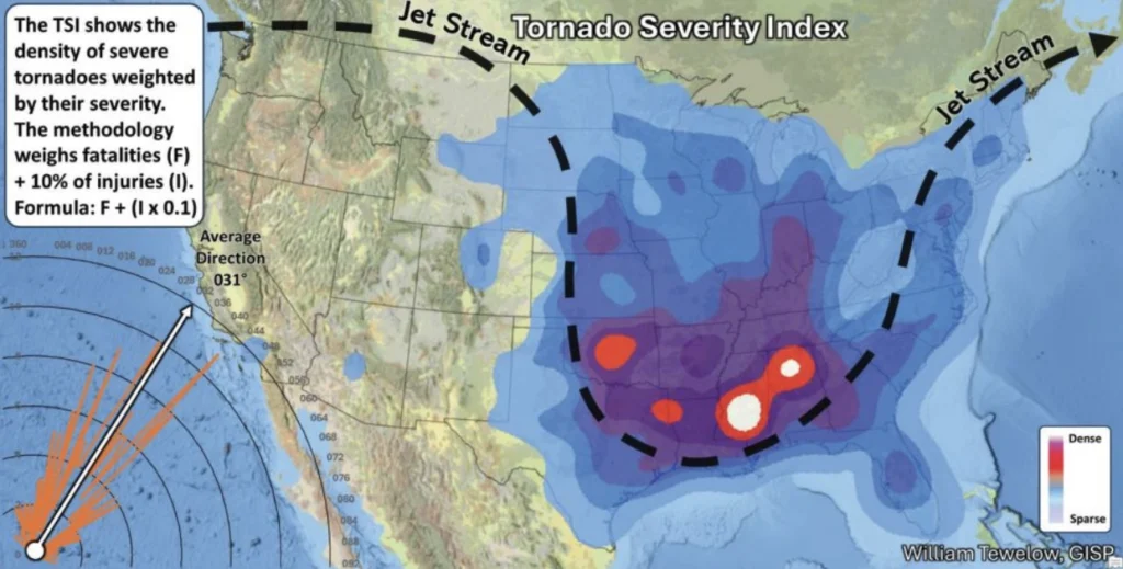
The question the rest of us ask from a safer distance is: What is the true pattern of destruction across time and geography? To answer it, I built a Tornado Severity Index (TSI) using National Weather Service tornado data. On average, there are 970 tornadoes per year, 81% are EF0 and EF1; 18% are EF2 and EF3; and the catastrophic EF4 and EF5 make up 1%.
The NWS database reports the start and end coordinates, path width, magnitude, fatalities, injuries, and damages to property and crops. Working with the coordinate pairs, I calculated the distance and radial bearing of each path. But the EF scale alone tells only part of the story: A powerful tornado crossing an empty field and a moderate tornado crossing a dense neighborhood are not equivalent human events.
I did not want the TSI to be another version of the EF scale, so the weighting was based entirely on the human toll. The formula is total fatalities (F) at 100% plus injuries (I) at 10%, =F + (I x 0.1) and normalized on a scale of 1 to 100. Economic damage was originally part of the equation, but the data are inconsistent and unreliable across reporting jurisdictions.
FIGURE 3 The Tornado Severity Index (TSI) takes the human cost into account. (Credit: William Tewelow)
The resulting composite doesn’t measure the strength of tornadoes, but rather their human impact (see FIGURE 3). The dataset of tornadoes from 1950 to 2024 is 71,813. Filtering it down to those tornadoes that had a human consequence where the TSI>1 reduced it to 2,362 tornadoes. I reduced it further to 1,625 including only those with one or more fatalities. This was made into a heatmap. The data were further reduced to 301, only filtering out all except where TSI>10. The heatmap color scale was weighted to the TSI Score. It shows where the highest concentration of intense tornadoes occurs.
The results confirm Tornado Alley from Texas up through Oklahoma, and it also reveals Dixie Alley, an even more destructive corridor of severe tornadoes over Mississippi, Alabama and Tennessee. These areas align with the deep spring meridional jet stream discussed earlier. The northern side of the jet stream enhances cyclonic flow for storms in the area. The peak region of vorticity is where the jet stream turns back north again over Dixie Alley. Additionally, the rising terrain in that area causes orographic lifting and more rain, many times hiding the tornadoes within the pouring rain.
GIS reveals what the physics predict: a narrow corridor of atmospheric geometry where conditions for catastrophic tornadoes are optimized, running through the same communities, year after year.
For the sake of context, the Joplin, Missouri tornado on May 22, 2011, that caused 158 fatalities, 1,150 injuries, and damages of $2.8 billion ranks at the top of the TSI. The Moore tornado only scored 16.6 due to far fewer fatalities.
The dataset reveals the physical signatures of severe tornadoes. On average, they peak in mid-May at 5:30 p.m. with a strength of EF4.2, carve a path 36 miles long and 2,073 feet wide, and each one causes 13 fatalities, 173 injuries, and losses of $71.5 million. Severe tornadoes do not travel west. They do travel a spectrum where most of them fall within a range from 016° to 060° with an average path of travel northeast at 031°. This is why Scott was right to question the reports of the El Reno tornado tracking southeast: What appeared to be southward motion was lateral growth. The tornado was not moving south; it was becoming enormous.
“Pretty much sucking everything up,” Scott said, with confidence born out of his experience.
The pattern and the person
The TSI heatmap is a record of moments like Scott’s, representing a convergence of humans caught up in brutal atmospheric physics, where air becomes violent. The science explains the experience. It cannot prevent the next EF5; the thermodynamics will prevail.
What GIS adds is pattern, memory and prediction. The TSI with directional analysis gives emergency managers, planners and underwriters insights for understanding where storm physics and humans intersect most acutely, and therefore where shelter codes and warning systems must be most robust.
The family in their shelter, watching the white dot approach on the glowing screen, is experiencing the culmination of decades of geospatial and meteorological investment: NEXRAD networks, GNSS constellations, real-time data fusion in a consumer app. But as Scott will tell you, the most important instrument was the steel latch on the shelter door, and what mattered most was the neighbor who held it open for him as the tornado approached.
Tornadoes are Earth’s thermodynamic engines of absolute chaos.
“I’m not interested in tornadoes,” Scott told me. “Once burnt, you don’t play with the matches anymore.”
Scott moved out of Oklahoma in 2013. The science is fascinating. People press right up to the edge of it, but the experience when science becomes personal is sheer terror.
Live tracking tornadoes with GIS census tracts can know in real-time the impact on populations to immediately begin rescue operations, clean-up and recovery.
GIS cannot capture the whirlwind, but it can track the most violent of them: northeast at 031°, seven football fields wide for 36 miles.
The market for mid- and high-precision GPS receivers is set to experience significant expansion in the coming years. Driven by evolving technologies and growing applications across various sectors, this market is attracting substantial attention, according to The Business Research Company.
The market size for mid- and high-level precision GPS receivers is expected to reach $6.85 billion by 2030, expanding at a compound annual growth rate (CAGR) of 12.2%. This robust growth over the forecast period is fueled by advancements in autonomous vehicle systems, expanding smart infrastructure projects, the rise of precision agriculture, increased use of highly accurate mapping solutions, and wider adoption of sophisticated GNSS correction services.
Important trends shaping the market include the pursuit of centimeter-level positioning accuracy, the integration of RTK and PPK technologies, use of multi-frequency signal processing, compatibility with survey software, and enhanced GNSS mapping precision.
The market features numerous influential companies, including Stonex Group Inc., Raytheon Technologies Corporation, Hexagon AB, Trimble Inc., Topcon Positioning Systems Inc., u-blox AG, Hi-Target Surveying Instrument Co. Ltd., CHC Navigation Technology Ltd., Carlson Systems Holdings Inc., Septentrio N.V., Hemisphere GNSS Inc., Javad GNSS Inc., Swift Navigation Inc., Thales Group, Geneq Inc., South Surveying & Mapping Technology Co. Ltd., Tersus GNSS Inc., Eos Positioning Systems Inc., NavtechGPS Inc., Satlab Geosolutions AB, Tallysman Wireless Inc., Leica Geosystems AG, NovAtel Inc., Spectra Precision, Unistrong Science & Technology Co. Ltd., and ComNav Technology Ltd.
Notably, in March 2023, Netherlands-based CNH Industrial N.V., a provider of agricultural and construction equipment as well as precision automation solutions, acquired Hemisphere GNSS for $175 million. This strategic move aims to combine Hemisphere’s high-precision GNSS receivers and satellite-based correction technologies with CNH’s capabilities to enhance machine control, autonomy, and positioning in both construction and agricultural sectors. Hemisphere GNSS, headquartered in the U.S., supplies advanced GNSS receivers, antennas, and correction services tailored for surveying, machine control, agriculture, and marine uses.
Top companies in this sector are actively launching new products to maintain competitive advantage.
For example, in October 2025, Unicore Communications Inc., a China-based GNSS technology provider, introduced the UM98XC Series-a next-generation, all-constellation, multi-frequency RTK GNSS module. Supporting GPS, BDS, Galileo, GLONASS, and QZSS systems along with L-Band and CLAS correction services, the UM98XC offers centimeter-level positioning accuracy. It also features advanced anti-jamming capabilities, energy-efficient design, and consistent performance in challenging environments, making it well-suited for autonomous driving, precision agriculture, unmanned aerial vehicles, and smart transportation sectors.
This launch underscores Unicore’s commitment to pushing the boundaries of GNSS precision, reliability, and scalability for industrial and automotive applications.