ZED-X20P-01B adds Galileo High Accuracy Service (HAS), Moving Base, and stronger resilience against jamming and spoofing, enabling scalable high-precision positioning for global OEM deployments.
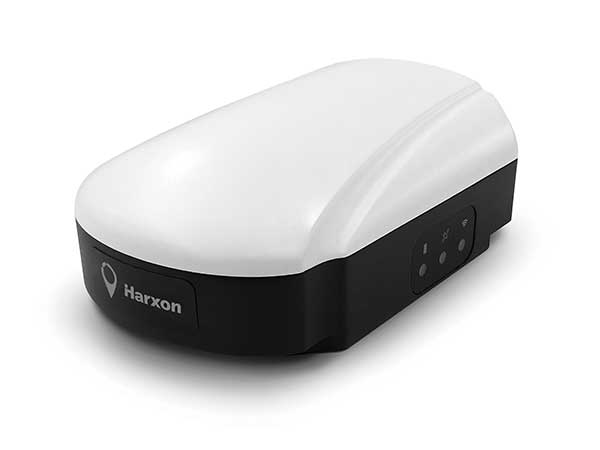
U-blox has launched and availability of its new all-band GNSS module variant, the ZED-X20P-01B.
Building on the proven capabilities of the ZED-X20P platform, the new module expands access to high-precision positioning by bringing global precise point positioning (PPP) to a broader range of use cases. With support for Galileo High Accuracy Service (HAS) the ZED-X20P-01B enables OEMs to launch products with reliable, decimeter-level positioning across markets worldwide, without tying product availability to local correction infrastructure.
The ZED-X20P-01B extends u-blox expertise in GNSS by addressing a growing market need: making high-precision positioning more practical to deploy at global scale. By integrating enhanced PPP capabilities, including Galileo HAS functionality, and improving resilience against jamming and spoofing (verified at Jammertest 2025), the module gives developers a dependable positioning that can serve both as a primary global solution and as a fallback where local RTK correction services are limited, unavailable, or impractical. This flexible approach opens new opportunities for global OEMs to design and ship products with reliable decimeter-level accuracy out of the box across regions, applications, and operating conditions.
The ZED-X20P-01B. (Credit: U-blox)
Built for global OEM deployment
The ZED-X20P-01B is especially valuable for products shipped across regions with inconsistent access to RTK networks, SBAS coverage, or reliable communications. This gives manufacturers a more flexible path to delivering high-precision positioning worldwide, while also opening new opportunities in remote, rural, and infrastructure-limited environments.
Representative applications include:
UAVs without reliance on continuous connectivity for mapping and navigation:
Marine applications such as dredging, near-shore navigation, and seabed mapping without complex RTK setup
Precision agriculture, construction and mining in remote locations, including geofencing and equipment tracking
Environmental and utility mapping in infrastructure-limited regions
Robotics and autonomous platforms requiring reliable relative positioning through Moving Base functionality.
Enhanced performance and robustness
The ZED-X20P-01B builds on the core strengths of the ZED-X20P while introducing key enhancements:
Native support for Galileo HAS for globally accessible PPP corrections
Moving Base functionality for applications requiring precise relative positioning
Improved jamming and spoofing detection and mitigation for mission-critical applications
Continued compatibility with u-blox PointPerfect services for scalable correction options.
Together, these enhancements help OEMs deliver reliable high-precision positioning across wider geographies and more demanding RF environments, while keeping system design streamlined. Most importantly, they make decimeter-level accuracy out of the box a practical option for products deployed globally.
Ease of integration and scalability
Maintaining the established ZED form factor, the ZED-X20P-01B offers a seamless upgrade path for existing customers. With its compact design it reduces the need for additional hardware or complex host-side computation.
This helps developers accelerate time to market and scale from pilot projects to global commercial rollouts without redesigning their systems for each target region. For OEMs building products for international shipment, the ZED-X20P-01B offers a practical way to standardize around one high-precision platform while expanding coverage, improving resilience, and simplifying deployment.
“ZED-X20P-01B reflects our commitment to making high-precision positioning more scalable, resilient, and easier to deploy globally,” said Andreas Thiel, CEO of u-blox, said. “With Galileo HAS support, Moving Base, stronger protection against jamming and spoofing, and a seamless path for existing ZED-X20P customers, we are enabling OEMs to bring reliable decimeter-level positioning to more products, in more markets, with fewer deployment constraints.”
Experience ZED-X20P-01B live
U-blox will showcase the ZED-X20P-01B at XPONENTIAL 2026 in Detroit, where visitors can experience the module live at booth 23023.
Availability
Samples and evaluation kits for the ZED-X20P-01B will be available in June.
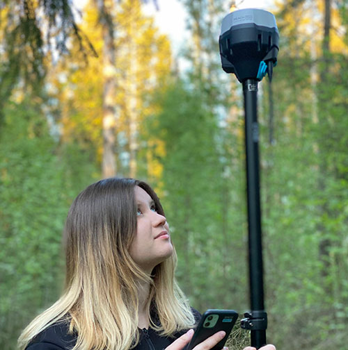
During a recent infrastructure survey, a handheld scanning system captured a multi-acre property in less than 15 minutes. As the operator moved through the site, the device continuously scanned the environment while maintaining centimeter-level positioning using satellite signals, inertial sensors and lidar.
The result was a fully georeferenced three-dimensional dataset containing terrain, buildings, trees and infrastructure — captured in a fraction of the time required by traditional survey workflows. Technologies such as these illustrate how far positioning systems have evolved. What once required multiple instruments, control networks and extended field observation can now be accomplished through integrated sensing systems combining satellite navigation with reality capture.
Yet, the foundation of these capabilities traces back more than six decades. Today, billions of devices depend on GNSS positioning. Smartphones, vehicles, aircraft, agricultural equipment and industrial systems rely on satellite signals to determine location and synchronize time. Within the geospatial industry, GNSS has evolved beyond navigation. It now serves as the spatial framework anchoring a growing ecosystem of sensors and measurement technologies capable of capturing the physical world in extraordinary detail.
Receiver evolution and productivity
While satellite constellations and positioning algorithms have steadily improved, many of the most noticeable changes for surveyors have occurred in the instruments themselves.
Modern GNSS receivers are smaller and more efficient than earlier generations. Advances in electronics, antenna design, signal processing and battery technology have reduced size and power requirements while improving reliability and usability in the field.
According to Chris Pappas, owner of Green Forest Surveys and a geospatial thought leader, recent GNSS receiver development has focused on usability rather than increases in raw positioning accuracy.
“What I’ve seen lately is smaller receivers, longer battery life and smaller antenna sizes on the heads,” Pappas said. “The quality has basically remained the same.” These improvements may appear incremental, but they have meaningful impacts on field operations.
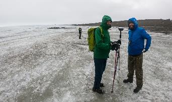
Survey crews work in demanding environments such as steep terrain, construction sites, transportation corridors and remote infrastructure locations where equipment weight and power management affect productivity.
“It’s portability. It’s fatigue from walking up a hill,” Pappas explained. “And the= longer battery life means you don’t have to constantly swap batteries or carry extras. You can take a single set with you and it’ll last all day.”
Modern receivers also have benefited from advancements in satellite signals and correction services. Today’s survey-grade receivers routinely track multiple frequencies from multiple constellations.
Miniaturization is not simply a reduction in size. Achieving multi-constellation tracking, multi-frequency processing and real-time correction required major advances in RF engineering and integrated circuit design.
Capabilities that once required large, power-intensive hardware platforms are now integrated into compact receivers capable of operating an entire day on a single charge.
Signal modernization, algorithms and the RTK engine
While receiver hardware has become smaller and more power-efficient, some of the most significant advancements in GNSS performance have occurred in the algorithms and processing engines operating inside those devices.
Modern receivers are specialized computing platforms designed to process signals from multiple constellations, frequencies and correction sources simultaneously. Tracking multiple constellations enables receivers to observe dozens of satellites while reducing ionospheric and multipath errors.
The real breakthrough, however, has come from improvements in the RTK engine itself.
RTK positioning relies on resolving the carrier-phase ambiguities — the unknown integer number of wavelengths between the satellite and the receiver. Earlier RTK systems often required extended initialization periods.
Modern receivers use more sophisticated ambiguity resolution algorithms that leverage multi-frequency observations and improved statistical modeling. Initialization times have dropped, and solutions are more robust in difficult environments.
Modern RTK engines incorporate advanced filtering techniques, stochastic modeling and automated outlier detection to maintain stable solutions when individual observations become unreliable.
These improvements are particularly important as surveyors increasingly work in environments where GNSS conditions are less than ideal. Urban infrastructure, tree canopy and industrial facilities can obstruct satellite signals and introduce multipath errors.
Advanced filtering architectures allow receivers to reject corrupted observations while maintaining stable positioning using valid measurements.
Many modern receivers incorporate Kalman filtering frameworks that continuously estimate position, velocity, clock bias and measurement uncertainties.
These filters allow GNSS measurements to be integrated with inertial sensors and motion constraints, creating more stable positioning solutions.
Network-based correction services also have become increasingly common. Rather than relying solely on a nearby base station, many surveyors now use network RTK systems that aggregate observations from multiple reference stations across a region.
These networks model atmospheric errors and deliver corrections through cellular or internet connections.
Precise point positioning (PPP) techniques, which use precise orbit and clock information rather than local base stations, also have matured significantly. Modern PPP engines can now resolve centimeter level positioning in real time or near real time, something that only a few years ago could take up to an hour using satellite based augmentation.
These advances have been enabled by the evolution of GNSS chipsets. Modern receivers integrate RF front ends, signal processors and navigation engines into compact system-on-chip architectures capable of tracking dozens of signals while running complex positioning algorithms in real time.
The result is a positioning engine that is no longer confined to a single receiver mounted on a survey pole, but operates as the central reference system for a network of sensors capturing complex environments.
The maturity of the modern positioning engine
One of the less visible but most important developments in GNSS over the past decade is the maturation of the positioning engine itself. Early GNSS receivers were essentially signal trackers paired with simple navigation algorithms. Today’s receivers function more like specialized computing platforms optimized for real time estimation.
At the core of these systems is an estimation framework that continuously evaluates the quality of each observation entering the solution. Carrier phase measurements provide the highest precision available from GNSS, but are highly sensitive to noise, multipath and signal interruptions.
Modern RTK engines must balance precision with reliability. Rather than assuming every observation is equally valid, processing engines assign dynamic weights based on signal strength, satellite geometry, atmospheric models and measurement stability. These approaches allow receivers to maintain accurate positioning even when portions of the satellite environment become unreliable.
Solar storms, such as this one in North Carolina, produce beautiful auroras. They also cause signal disruption and interference for GNSS systems. Many of the modern RTK engines now have the ability to filter out this interference and maintain a fix.
The introduction of multi frequency signals also has changed how ambiguity resolution is performed. Earlier RTK systems relied on dual-frequency measurements to estimate ionospheric delay and resolve integer ambiguities. With additional frequencies across multiple constellations, modern receivers apply more advanced ambiguity resolution strategies that improve convergence speed. In practical terms, this means surveyors spend less time waiting for initialization and more time collecting data.
Modern receivers also incorporate tightly integrated filtering architectures. Extended Kalman filtering frameworks continuously estimate position, velocity, clock bias, atmospheric parameters and measurement noise. These models treat positioning as a dynamic estimation problem rather than a static calculation performed at each epoch. The result is a positioning engine capable of maintaining stable centimeter level solutions even when signal conditions fluctuate. For surveyors working in environments with partial satellite obstruction, intermittent multipath or complex site conditions, these improvements often determine whether a day in the field is productive or not.
GNSS as foundational infrastructure
Today, GNSS occupies a unique position in the technology landscape. It is both a mature infrastructure system and a platform for continued innovation. The fundamental architecture of satellite navigation has remained largely consistent for decades, while the ecosystem built around those signals has expanded dramatically.
In many ways, GNSS has become invisible because it works so well. Surveyors, engineers and geospatial professionals interact with receivers, correction services and data products rather than with the satellites themselves. Positioning is expected to function, much like electricity or cellular connectivity. But under that routine operation lies one of the most sophisticated global infrastructure systems ever constructed.
At the space segment level, multiple international constellations provide overlapping coverage. The United States’ GPS, Russia’s GLONASS, Europe’s Galileo and China’s BeiDou systems transmit modernized signals designed to improve accuracy, reliability and interoperability. Regional systems such as Japan’s QZSS and India’s NavIC further strengthen coverage.
This multi-constellation environment represents one of the most significant changes in the GNSS landscape throughout the past two decades. Early survey grade receivers relied primarily on GPS signals, while modern receivers track four or more global constellations simultaneously.
The impact extends beyond redundancy. Observing more satellites improves geometric strength and allows receivers to maintain robust solutions in environments where single constellation systems would struggle, including urban corridors, forested areas and complex infrastructure sites.
Signal modernization has expanded the range of measurements available to positioning engines. Additional civilian frequencies such as GPS L5 and Galileo E5 allow better modeling of ionospheric effects and reduced measurement noise, contributing to more stable positioning solutions.
The most important shift, however, is not in the satellites themselves, but in GNSS’s role within the broader measurement ecosystem.
In the surveying and geospatial industries, GNSS has evolved from a standalone measurement technique into the spatial reference framework for modern data capture technologies. It now anchors measurement platforms capable of capturing millions of spatial observations.
In traditional surveying, GNSS remains a primary method for establishing control networks and geodetic reference points, with RTK and post-processed kinematic techniques routinely achieving centimeter-level accuracy.
In construction and machine control, GNSS enables automated positioning systems that guide heavy equipment using digital terrain models in real time.
In agriculture, precision farming systems use satellite positioning to guide equipment along exact paths, reducing fuel consumption and optimizing inputs.
GNSS also functions as the primary time synchronization system for critical infrastructure, including telecommunications, financial systems and power grids.
For geospatial professionals, the most significant change is how GNSS interacts with emerging measurement technologies. Rather than acting as a standalone sensor, it now operates as the global reference frame for integrated systems.
The satellite-derived position establishes a coordinate foundation that other sensors use to build dense spatial models. In a typical workflow, GNSS establishes the reference, inertial sensors track motion, lidar captures geometry and cameras record imagery. All observations rely on the GNSS reference frame to maintain spatial consistency.
This enables a shift from discrete point measurement to continuous data capture. Instead of collecting individual points, modern platforms capture millions of observations that can be analyzed and extracted as needed.
GNSS remains the backbone of this process. Even as new sensors emerge, the requirement for a stable global reference frame has not changed. GNSS provides that anchor.
Sensor fusion and the expanding positioning stack
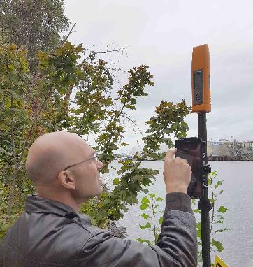
While GNSS technology continues to evolve, some of the most significant advances in positioning are occurring through integration with other sensing technologies.
Trees, such as this 150-year-old tulip poplar, were killers of previous-generation GNSS systems. Robust designs, the modern sensor stack, and powerful algorithms can now fix reliably in heavy canopy, saving hours of traditional work.
Modern positioning systems operate as part of a broader sensor ecosystem. Satellite observations provide the global reference frame, while inertial measurement units track motion and orientation, lidar sensors capture geometry and visual sensors analyze environmental features.
Hybrid platforms extend GNSS capability into environments where satellite signals alone may struggle. Several manufacturers now offer handheld systems that combine GNSS receivers with lidar scanning and inertial navigation. Systems such as the CHC Navigation VLi100 integrate GNSS, lidar, inertial sensing and visual positioning into a single instrument. The VLi100 also incorporates the SureFix 2.0 engine, which uses lidar to stabilize the GNSS position for up to 60 ft after signal loss, extending positioning capability in obstructed environments.
The Tersus S1 SLAM system similarly combines lidar-based mapping with GNSS positioning to capture dense spatial data in complex environments.
The same principles drive mobile mapping systems designed for infrastructure-scale data capture. Trimble’s MX series, including the MX9 and MX90, combines GNSS positioning, high-accuracy inertial navigation and high-density lidar to capture detailed spatial data while in motion.
“Sensor fusion is probably the biggest one right now,” said Justin Brooks, sales manager for reality capture at Trimble. “When you combine GNSS with lidar and inertial sensors, you’re not just collecting points anymore. You’re capturing entire environments.”
Mobile mapping is increasingly used across the energy sector. According to Jason Rosbach, director, energy solutions at Trimble, large renewable energy projects such as utility scale solar and wind developments require rapid spatial documentation across thousands of acres. These systems allow survey teams to capture dense geospatial datasets while maintaining consistent positioning through tightly integrated GNSS and inertial navigation.
Karl Bradshaw, director, product management, reality capture at Trimble, explained that GNSS remains the core reference.
“In the MX systems, that GNSS position is the initial core point,” Bradshaw said. “Then the IMU interpolates the vehicle path between those GNSS fixes and provides heading, pitch and roll orientation. Every lidar pulse gets geolocated using that combined solution.”
Reality capture and the GNSS positioning pyramid
The convergence of GNSS positioning with lidar scanning, inertial navigation, and SLAM-based mapping is driving the broader adoption of reality capture workflows across the geospatial and infrastructure industries.
At the core of these systems remains a GNSS-centric positioning pyramid. Satellite observations provide the spatial reference that anchors all other measurements. The additional sensors extend and stabilize that position when conditions become challenging.
From point measurement to spatial data acquisition
The integration of GNSS with modern sensing technologies has changed the scale of spatial data collection.
For most of the 20th century, surveying workflows were based on discrete point measurements. Whether using optical instruments, total stations or early GNSS receivers, surveyors collected individual observations that were later combined to construct maps and models.
This approach remains essential for control networks and boundary surveys, but many modern applications now operate at a fundamentally different level of data density.
Lidar scanners, mobile mapping systems and handheld SLAM platforms can collect millions of measurements in minutes. Instead of selecting points, operators move through an environment while continuously capturing geometric observations. These datasets provide a far more detailed representation of the physical world.
GNSS enables this transition by providing a stable global reference frame. Without it, large point clouds and reality capture datasets would exist only as isolated local models. GNSS allows these datasets to align with engineering design files, geographic information system (GIS) databases and previous survey measurements.
This spatial consistency makes reality capture practical for large infrastructure projects. Transportation departments can compare roadway conditions over time, utilities can integrate asset models and construction teams can verify progress against design.
In each of these workflows, GNSS provides the coordinate framework that keeps datasets aligned across time, sensors and project stages.
The shift from point measurement to continuous data acquisition is one of the most significant changes in geospatial practice in decades.
Even within these systems, positioning still begins with satellite signals. GNSS remains the foundation. Lidar captures geometry, inertial sensors measure motion and SLAM algorithms track environmental features, all fused with the GNSS position.
These systems collect dense spatial observations continuously, allowing entire corridors, facilities and infrastructure sites to be captured rapidly. Because these datasets are anchored to GNSS positioning, they maintain consistent spatial reference over time.
Looking ahead
Another development drawing increasing attention across the positioning industry is the emergence of low Earth orbit (LEO) satellite constellations as potential complements to traditional GNSS systems.
Unlike GNSS satellites operating at medium-Earth orbit altitudes of roughly 20,000 kilometers, LEO satellites orbit much closer to Earth. This proximity allows their signals to reach receivers with significantly higher signal strength and faster acquisition times.
Because the satellites move rapidly across the sky, they also provide constantly changing geometry that can improve positioning performance in environments where traditional GNSS signals struggle.
A number of research groups and commercial companies are now exploring how LEO constellations might augment existing GNSS infrastructure. Some approaches rely on signals from existing communications constellations, while others involve dedicated navigation payloads designed specifically for positioning.
For surveyors and geospatial professionals, the potential benefit is improved positioning reliability in environments where GNSS signals are degraded. Urban corridors, industrial sites and areas with heavy canopy often limit satellite visibility and introduce multipath interference that complicates carrier-phase measurements.
Additional signals from LEO satellites could provide stronger observations in these environments while also improving the redundancy of positioning solutions.
The integration of LEO signals would not replace GNSS but rather expand the broader positioning ecosystem that already has begun to emerge through sensor fusion.
Modern positioning systems increasingly combine GNSS, inertial navigation, lidar, camera and SLAMbased mapping into tightly integrated sensor stacks. GNSS provides the global reference frame, while the other sensors extend and stabilize the positioning solution when satellite visibility becomes limited.
If LEO navigation signals become widely available, they will likely become another layer within that stack.
The long-term result could be positioning systems capable of maintaining centimeter-level trajectories across environments that would have been extremely difficult for GNSS-only solutions just a decade ago.
For the geospatial industry, this evolution represents a continuation of a trend that began decades ago: positioning systems becoming more robust, more integrated, and increasingly capable of capturing the physical world in unprecedented detail.
Multinational technology firm GMV has signed an agreement with Lockheed Martin Corporation to develop the processing and control centers for the Southern Positioning Augmentation Network system (SouthPAN). Lockheed is contracted to establish SouthPAN.
The project is a joint initiative of the Australian and New Zealand governments to provide a satellite-based augmentation system (SBAS) for navigation and precise point positioning (PPP) services. GMV will also be responsible for monitoring both of these services in the region and for ensuring compliance with the committed performance levels.
SBAS and PPP systems have applications in industries as diverse as agriculture and road, air, maritime and rail transportation, as well as in the field of geomatics. SouthPAN is expected to accelerate development of applications in these areas.
SouthPAN is also the first system with these characteristics available in the Southern Hemisphere. With this new program, Australia and New Zealand will be contributing to improved global coverage and interoperability for services of this type, joining the list of countries and regions that already have their own SBAS system: the United States (WAAS), Europe (EGNOS), India (GAGAN) and Japan (MSAS).
On Sept. 26, two weeks after the agreement was signed, the first services were provided by activating transmission of the system’s first signals. This was a significant milestone, because SouthPAN is the first project where an industry consortium provides an SBAS as a service, rather than as a turnkey system.
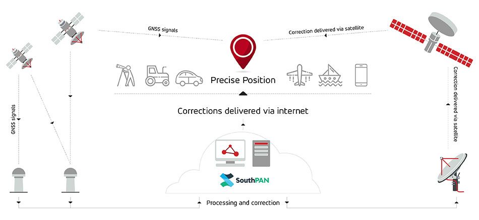
Image: SouthPAN
GMV’s role
GMV will be responsible for developing two key subsystems for SouthPAN: the Corrections Processing Facility and the Ground Control Center. The company will also be responsible for monitoring the system and ensuring it complies with the committed performance levels.
GMV also will provide support for the system’s operation and maintenance.
Corrections Processing Facility. The facility generates correction messages for signals transmitted by GPS and Galileo, improving precision for users by improving accuracy to as little as 10 centimeters.
The facility also detects malfunctions in the satellites and generates warnings for users. This will allow use of SouthPAN by civilian aircraft as a navigation system during various flight operations, including precision approaches to runways for landing.
Safety-of-life services such as these will be available in 2028.
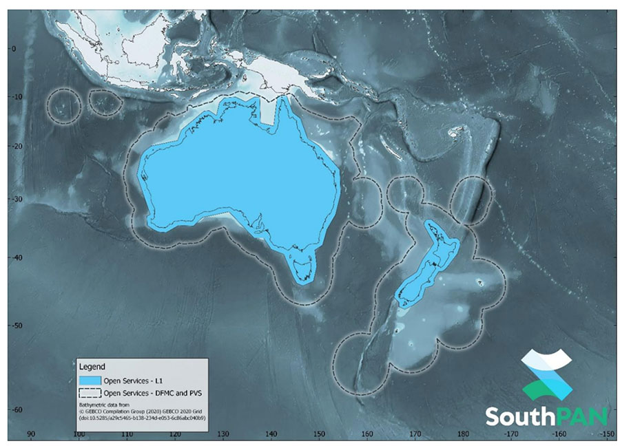
SouthPAN early Open Services coverage. OS-L1 covers mainland Australia and New Zealand. OS-DFMC and OS-PVS cover Exclusive Economic Zones in both countries. (Image: Geosciences Australia)
Ground Control Center. The control center remains in operation 24 hours a day seven days a week, and will perform all the functions needed to monitor and control the system. It will also provide information to users about the system’s operation and availability of services.
In Australia, SouthPAN development, entry into service and operation are being supervised by Geoscience Australia in collaboration with Toitū Te Whenua Land Information New Zealand.
In 2020, the two agencies signed the Australia New Zealand Science, Research and Innovation Cooperation Agreement (ANZSRICA). Over the next 20 years, the Australian government will be contributing 1.4 billion Australian dollars to the SouthPAN project.
Trimble has introduced data integrity monitoring for CenterPoint RTX Fast, its precise point positioning (PPP) correction service.
The Trimble RTX Integrity monitoring system is an innovative, patented solution, built in direct response to client requirements for production-ready applications. It continuously validates the reliability of correction data processed by the network, which is broadcast to users in the agriculture, geospatial, construction and automotive industries, ensuring positioning data is right the first time.
Through a two-step process, the Trimble RTX Integrity system verifies the integrity of GNSS data and filters faulty information in the network server before the data is broadcast. A secondary post-broadcast check is conducted on the entire data transmission process where additional errors may be detected and removed.
The integrity monitoring system is fully automated and reacts in seconds to detect, isolate and block faulty data to provide even more highly accurate and reliable positioning.
Trimble RTX Integrity is comprised of independent monitoring stations strategically positioned across RTX Fast networks in the United States, southern Canada and across Europe. These stations continuously monitor data output during multiple stages of the Trimble RTX positioning process. Any suspicious satellite data is removed during the integrity protection process and positioning is calculated using only validated data.
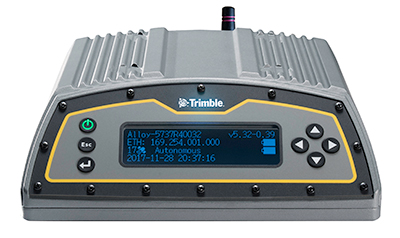
Trimble Alloy GNSS reference receivers power the independent monitoring stations using redundant internet connectivity for added reliability. To date, no other positioning network offers the same level of data integrity validation across such expansive, contiguous geographies.
Trimble RTX Integrity monitoring system was developed in accordance with Automotive Software Performance Improvement and Capability dEtermination (ASPICE) and ISO 26262 automotive safety standards, making it easy to integrate into major automotive manufacturers’ autonomous driving systems.
Trimble RTX Integrity can also be used by Trimble’s customers in the agriculture, geospatial and construction industries to ensure correction stream integrity and reliability for applications such as machine control and high-accuracy surveying applications.
“Trimble remains committed to exceeding expectations by providing accurate corrections to our customers to support safety-critical and other day-to-day applications,” said Patricia Boothe, SVP of autonomy, Trimble. “Implementing additional checks and balances to ensure our data is authenticated, trustworthy and accurate is of paramount importance to maintaining the integrity of our RTX network and instilling confidence with our users that the data is correct.”
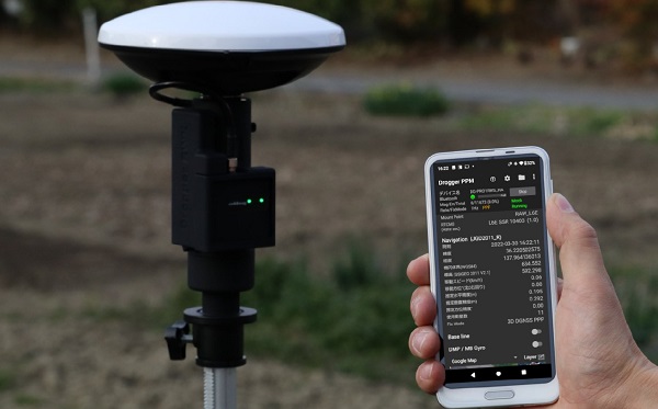
BizStation, a database company based in Japan, and u-blox have announced a highly accurate, compact and low-cost high-precision positioning solution for markets in East Asia and Oceania.
Featuring two u-blox modules, the solution delivers centimeter-level positioning accuracy where mobile network service is unavailable, including in maritime offshore surveying, agricultural and industrial vehicle guidance, and UAVs.
BizStation’s precise point positioning (PPP) system covers all territories served by Japan’s Quasi-Zenith Satellite System (QZSS) MADOCA correction service.
The solution leverages the strengths of two u-blox components. The first, a u-blox ZED-F9P multi-band high precision GNSS receiver module, is at the heart of BizStation’s DG-PRO1RWS GNSS receiver.
The second, a u-blox NEO-D9C correction-data receiver module specific to Japan, enables their virtual reference station to receive data on the QZSS L6E-band used by MADOCA.
The PPM (PPP positioning by MADOCA) Android application developed by BizStation then determines the location of the tracked device using the high-precision positioning data transferred via Wi-Fi from BizStation’s DG-PRO1RWS GNSS receiver as well as GNSS correction data from the virtual reference station. The PPM application performs all required calculations using the MADOCA positioning library developed by NEC Solution Innovators Co., Ltd.
The high-precision GNSS solution can be deployed either using a static or a mobile virtual reference station for a wide range of applications such as agriculture, drones, motor sports or surveying systems.
A positioning service energizes large pipeline surveying projects, saves time, and becomes a field crew favorite
For projects spanning large areas, a large engineering and construction firm discovered that a precise point positioning (PPP) service — Trimble’s CenterPoint RTX — could solve the challenge of receiving high-precision GNSS in remote areas.
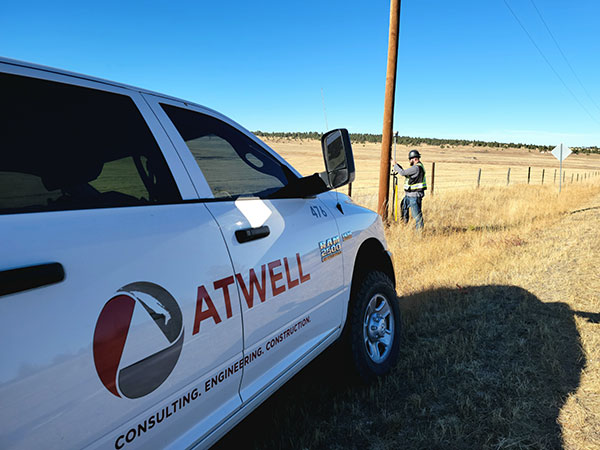
Atwell Group LLC is a national consulting, engineering and construction services firm with 33 offices throughout the country and more than 1,000 team members. The company delivers a broad range of strategic and creative solutions to clients in three core markets: oil and gas, power and energy, and real estate and land development.
Atwell provides comprehensive turnkey services, including land and right-of-way support, engineering, land surveying, environmental compliance and permitting, and project and program management.
Photo: Trimble
Pipeline construction
Atwell’s introduction to PPP and Trimble’s CenterPoint RTX took place during two large-scale linear pipeline projects within remote areas. Atwell has substantial experience with projects of this scale, but the remoteness of some of the projects’ sections was proving to be a challenge. While they could expect to rely on base or network correction methods for most projects, Atwell needed to seek other correction alternatives — and up their efficiency for the long-corridor projects.
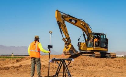
With the CenterPoint RTX service at hand, Atwell performed construction staking and as-built surveys for a 50-mile pipeline. The project spanned a five-month period, with an hour or more of time saved each day using the service.
Crews noticed an additional benefit: rapid response time. On any given day, there could be project managers, right-of-way agents, or inspectors on site, asking for additional survey data.
“Inspectors and others started to notice how fast our crews could jump from one place to another and get the shots they requested, without having to do any base setups,” said Jason Jung, project manager with Atwell.
“The speed at which our crews can get up and running with RTX is awesome.” — Jason Jung, 3D laser scanning projects manager, Atwell
Because of the range limits of base radios, the crews might have to do multiple setups of a conventional real-time kinematic (RTK) base each day. RTX removed this hindrance, saving the crews time by not having to use temporary RTK bases, which entails driving to base reference points, setup and teardown, and downtime from malfunctioning equipment and battery issues.
“RTX completely freed us from the time and hassle of base setups,” Jung said. “You turn it on, and it’s ready to go before you’ve had time to take a sip of coffee. And once our crews got used to it and gained confidence in the results, they have really loved this solution.”
Photo: Trimble
Scanning a pipeline
Atwell recently used CenterPoint RTX on a 135-mile large-diameter pipeline project that included 19 facilities along the route. Atwell provided as-built services related to the facilities using a Trimble X7 scanner.
The data captured was used to generate spatially correct site models that included the material traceability necessary to comply with Pipeline and Hazardous Materials Safety Administration (PHMSA) regulations. Crews used RTX to georeference point clouds from the scanner to provide the accuracy needed to comply with industry regulations. Each site was referenced with permanent monuments or scribes that tied into the master control system.
Crews also used the RTX service to establish hard checkpoints to meet Atwell’s strenuous quality-control requirements for ground targets, such as those used in UAS control work. To do the daily “in and out” check shots, they used the free BenchMap app to locate nearby survey control marks from the National Geodetic Survey database. Most checks were sub-0.08’.
The time saved in not having to change base positions, as well as setup and breakdown, were significant time savers along this lengthy project. The precisely registered scans helped speed up PHMSA required inspections and audits, and construction change management field operations.
A crew favorite
Atwell’s crews use Trimble R10 receivers and Trimble Access running on TSC7 controllers, but Jung noted that they have recently upgraded to some R12i GNSS receivers, “and they are already earning their keep.” He expects to realize even more benefits from RTX coupled with the advanced multi-constellation capabilities of the Trimble ProPoint RTK engine in the R12i.
RTX has not only become a crew favorite, it is fast becoming a go-to solution for many Atwell projects.
TerraStar-C PRO is the first global correction service from Hexagon to incorporate RTK From the Sky technology to achieve RTK-level accuracy in three minutes with 99.999% availability
In late 2020, Hexagon’s Autonomy & Positioning division announced its technological breakthrough of global RTK From the Sky, demonstrating a future where instantaneous PPP and global RTK-level accuracy is possible.
Integrating this innovation into the core of TerraStar-C PRO, NovAtel’s corrections service, is the first phase in implementing RTK From the Sky technology into the company’s diverse portfolio of correction services for users worldwide.
As a result, TerraStar-C PRO has become the fastest global correction service to provide centimeter-level accuracy, not just in open-sky environments but also across challenging conditions created by buildings and foliage, according to Hexagon | NovAtel.
“RTK From the Sky technology is the foundation that enables our global correction services to be world-leading across agriculture, automotive, defense, survey, marine and autonomous applications,” said Michael Ritter, Autonomy & Positioning division president and CEO. “Our dedication to research culminated in an industry-changing technology; we’ll continue that commitment by providing the best positioning experience in speed, accuracy, availability and reliability anywhere in the world.”
TerraStar-C PRO now converges in less than three minutes by utilizing quad-band receiver and antenna technology to leverage modernized BeiDou III, GPS III and Galileo E6 signals. The resulting process generates state-of-the-art corrections for all GNSS frequencies.
Hexagon is a consistent innovator in GNSS, as seen in its role in developing RTK and PPP solutions. With this next-generation modernization of PPP correction generation and algorithm development, the company continues this tradition in providing the highest quality and best performing global positioning experience to users with land- and air-based applications.
“It’s been a privilege to collaborate across the division to develop RTK From the Sky technology and leverage our collective expertise in correction generation, PPP algorithms and the entire positioning ecosystem,” said Leos Mervart, head of PPP algorithm development at Hexagon’s Autonomy & Positioning division. “I’ve worked with PPP technologies since the beginning of my career and am proud to say that this is a new era of what global positioning can look like.”
The TerraStar-C PRO improvements are accessible now through the 7.08.10 firmware release for users on OEM7700, OEM719 and OEM729 cards and their associated enclosures for land and air applications.
Future firmware releases will include global RTK From the Sky technology throughout Hexagon’s correction service portfolios for its global client base, including precision agriculture and marine applications.
To learn more about TerraStar correction services or to request a free 5-day trial, visit NovAtel.com/TerraStar.
Approaches to providing real-time kinematic (RTK) solutions at high rates have existed in various forms for decades, providing value for high precision applications. This technique is nearly universally adopted in the industry, and many surveyors may have been using it for years without realizing it. Yet there are persistent misconceptions about the subject.
By Gavin Schrock, PLS
For many on the development side of high-precision real-time kinematic (RTK) GNSS, like those we interviewed for this article, the incorporation of high-rate solutions into their RTK products is a given — and has been for a very long time. Yet, in some end-user communities there may still be many question marks: Does my gear do it? Does other gear do it? What can it do for me? What are the pluses and minuses?
We asked for insights from 10 prominent firms that develop and manufacture RTK-enabled high-precision GNSS solutions and equipment, spanning multiple applications:
By high rate, we mean higher than 1 second (1 Hz) increments, such as 0.2 second (5 Hz), 0.1 second (10 Hz), etc. Part of the confusion about high-rate RTK is that there are two scenarios. One is transmitting corrections from a base or network at high rate, receiving and solving on-the-field sensors or rovers at a high rate (for example, 5 Hz base + 5 Hz rover).
The other is base transmission of corrections at a lower rate and receiving/solving on the rover at a higher rate (for example, 1 Hz on the base + 5 Hz or more on the sensor/rover).
While both can be valuable for different applications, what has been adopted as standard for most surveying, construction, agriculture and mapping applications is the latter.
What are applications that would run the base and rover at higher than 1 Hz? “Moving Base” applications are prime examples, where you are seeking to resolve positions for one or more sensors relative to a base that is also on a moving platform. Think of a barge on the ocean where a helicopter (or rocket) might be landing. Here is a definition from the user manual for a popular OEM receiver that has been in many makes and models since 2003:
“Moving Baseline RTK is an RTK positioning technique in which both reference and rover receivers can move. Moving Baseline RTK is useful for GPS applications that require vessel orientation. [For example, the] reference receiver broadcasts [correction] data at 10Hz, while the rover receiver performs a synchronized baseline solution at 10Hz. The resulting baseline solution has centimeter-level accuracy. To increase the accuracy of the absolute location of the two antennas, the Moving Reference receiver can use differential corrections from a static source, such as a shore-based RTK reference station.”
Beyond such specialized applications, running the base at a high rate is a burden on radios or bandwidth. Additionally, as industry experts explain below, it is of little (or no) value and may only unnecessarily use excess bandwidth and burden broadcast radios.
When would you run the base at 1 Hz and the rover at higher than 1Hz, such as 5Hz, 10Hz, or more? When the base is static. That pretty much covers nearly all surveying, mapping, precision agriculture and construction applications. What is meant by high rate in the sensor/rover receiver and its RTK engine, in the context of such applications? As one of the firms interviewed stated:
“The number of RTK position fixes generated per second defines the update rate.”
For most of the surveying, mapping, precision agriculture and construction applications, that means base 1 Hz + rover 5 Hz or 10 Hz. Then there are specialized applications, such as structural monitoring and geophysical studies, that may run sensors/rovers at 20 Hz, 50 Hz or (though rare) as high as 100 Hz. Whether a higher rate is a default, or 1 Hz is the default, changing the rate is almost always a user-configurable option.
A general perception is that base-rover gear defaults to base 1 Hz + rover 1 Hz. However, as the experts below note, that is not necessarily the case — often the rover rate is higher by default.
By any other name…
The respective approaches, and their appropriateness for different end-use applications, may seem fairly straight forward. However, part of the confusion about the subject for end users comes from the wide range of terminology used to describe how high rate is applied across the industry.
The understanding of processing approaches is clear among GNSS engineers, and in specific terminology, but this rarely gets translated well or consistently in terms meaningful to end users in documentation or marketing.
Developers might have different approaches to achieving high-rate solutions and would of course not wish to completely reveal their cards, but many of the fundamentals are the same. A mutual recognition of parallel development among GNSS engineers, and the manufacturers they develop for, in that each strives to continually improve solutions, means that the high-rate element of RTK generally does not get much marketing hype.
Often, when high-rate RTK does get laterally mentioned — in manuals, marketing or labeled as configuration options in GNSS field software — the mix of terms can confuse the user. Such terms as extrapolation, prediction, update rate and solution rate could evoke a negative connotation to an end user who is used to hearing one set of terms, and they might view otherwise like terms as contrasting terms.
GNSS engineers do not have issues with mixed terms. As some indicated in their respective interviews, they seem a bit puzzled as to why anyone would misunderstand the subject, and how marketing spin might lead users to be confused.
In recent years, the subject seemed to get discussed a lot more than usual in various high-precision end-user social media platforms. Perhaps this was a natural progression in growth of understanding of the nature of GNSS among these constituencies, and a desire to know more about what goes on in those black boxes — a positive thing. There may also have been some instances of marketing nudge.
For whatever reason it became a subject of discussion, we heard from readers who asked us to look into it. So here, in alphabetical order, are insights from of the experts in this field. You can jump ahead to the specific section for your equipment vendor, but we encourage you to read through each; combined, they provide a more complete picture of the subject.
Bad Elf
With Larry Fox, VP for Marketing and Business Development
Larry Fox uses the Bad Elf Flex. (Photo: Bad Elf)
Bad Elf has long provided GNSS solutions for aviation- and mapping-grade field applications. Several years ago, the company introduced a survey-grade-precision system, Flex. It is offered with an option for a modest initial investment in the hardware, and an innovative token system for enabling and operating at centimeter precision.
Larry Fox has been in the industry for a long time and has seen the evolution of real-time GNSS. He is Bad Elf’s vice president for marketing and business development, but he also had a key role in the development of the Flex system. Fox said that, of course, high-rate RTK is supported. “We allow options up to 20 Hz on the rover if the user has this enabled.”
For the approach of 1-Hz base and higher rates on the rover, he said that Bad Elf does not have a specific term for this. “For purposes of description, I could refer to it as high update rate, but I suspect high solution rate is pretty much synonymous.”
Fox explained how the standard approach works. “The rover knows the location of the fixed base and therefore applies the same processing techniques by simply reusing the last received data.”
He also mused about various hypothetical scenarios. “Given that the converse is also possible — a slow data rate from the base, say, 0.2 Hz at the base and 1 Hz at the rover — is there fundamentally any difference?”
For many applications, Fox does not see a substantial advantage in running at higher rates: “I see no benefit for higher data rates in a static situation such as a survey. I would argue that in a survey workflow, one should allow the RTK algorithm to settle over the static shot being taken, as the RTK algorithm likely benefits from aging out some of the data it used while moving.”
He adds, “I would suggest that once you have occupied a point for a modest amount of time and you remained fixed, I can’t see any benefit. My argument here is that by the time you have leveled and prepared your collector of choice, any decent RTK receiver with a good sky portrait and good corrections will not observe any benefit.”
As for disadvantages and trade-offs, “More and faster data,” Fox said, “must be better, correct? Sarcasm included. Unless there is a tangible need for more samples, what is one going to do with all the extra data? I could have seen a possible argument that a single constellation receiver may benefit from averaging, but that could be a be a whole different subject as multi-constellation is now standard. Arguably, at a higher data rate one could capture more epochs and reduce the time on station. With multi-constellation receivers I am just not convinced that these techniques have the same merit they may have had in the past.”
Bad Elf doesn’t support higher correction transmission rates from the radio. “The current module only supports RTCM3 at a 1Hz rate,” Fox said. “Even if we could transmit faster, the payload required would exceed the capability of the message transmission rate of the radio. The battery life of a radio is directly correlated to the transmission duty cycle. The more you are transmitting, the less battery life you will have. I would argue this would impact the useful field time you would have without an external battery solution.”
Fox notes that any application where a rover is moving — such as on a vehicle or for machine control — could benefit from high rate. “I could see a potential application for drones,” he added. “I would want to have the epoch of an image recording very tightly coupled to the image captured. Fundamentally, an RTK drone’s imagery is only as good as that. If one was taking video at any reasonable framerate, a higher frequency RTK GNSS may benefit the geolocation of more individual frames with less extrapolation.”
What about rates higher than 20 Hz? “We have run our receiver up to 20 Hz on the rover side. Although there are units capable of even higher rates, I don’t have any data that would convince me that this is viable, for mapping or surveying.”
I asked about some of the misunderstanding out there about high-rate RTK, and Fox replied, “We can be creatures of habit and tie ourselves to beliefs that ‘this is the way I did it and it worked then.’ People should always ask themselves the question, ‘do I still need to do it this way?’ Again, there is the premise that more is better. I can’t tell you how many times I have seen people collect very high-rate data for lines and poly features only to decimate the data because it reduced performance, increased storage, or lowered the performance of the apps rendering the data.”
Emlid
With Svetlana Nikolenko, Lead Application Engineer
Photo:Svetlana Nikolenko with an Emlid GNSS receiver. (Photo: Emlid)
Emlid, a relatively new entrant to the market for high-precision GNSS, has made a splash with their line of affordable systems, such as the Reach RS2 rover and base-rover kits, and RTK systems for UAVs.
“All our devices support this,” said Svetlana Nikolenko, lead application engineer. “We do not have a special term for this, as it is simply a standard. We recommend 5 Hz and higher for a moving rover, but it can be overkill for a stationary one.”
Asked why one would want to run at high rate, Nikolenko explained, “The need to set a higher update rate depends on the rover’s velocity and acceleration. The higher the update rate, the more solutions per second are calculated. So, if you’re moving fast, the higher update rate simply allows you to keep your position current. If the rover is stationary, there are no issues with working at 1 Hz. Still, there is nothing wrong with running a stationary rover at 5 Hz or higher: it is excessive, but produces more samples with different satellite geometries.”
For moving applications such as UAVs, higher rates are of value. “It really depends on velocity,” Nikolenko said. “For example, if the rover is on a drone flying at a speed of 5-20 m/s and the update rate is set to 1 Hz, you won’t have the actual positions of the images. The higher update rate our devices have is 10 Hz, and at a drone speed of 20 m/s, even if you take photos each second (which might be a bit excessive), you’ll get accurate positions.”
Using an Emlid receiver in harsh conditions. (Photo: Emlid)
Emlid does not support a moving base. However, if there is a strong demand from users, they will consider adding this. For non-moving applications, Nikolenko said, an approach of broadcasting from the base at a high rate is excessive. “This increases the load on the radio (or any other connection link) because the base sends its position and corrections to the rover as often as it calculates it. Anything excessive simply adds load to processors and batteries.”
CHC Navigation
With Carlos Cao, Technical Manager for the Asia-Pacific region
CHC Navigation, or CHCNAV, has steadily grown as a recognizable brand of GNSS and other geospatial products internationally. While the brand might be new to some in North America, in some regions of the world CHC has a substantial share of the market, selling hundreds of thousands of units over the past 15 years. The company develops its own solutions, but also incorporates OEM components. In all cases, CHCNAV has provided high rate as standard from its earliest days.
Multi-constellation rover with tilt compensation. (Photo: Schrock)
Carlos Cao, technical manager for the Asia-Pacific region, said that his company supports the approach of broadcasting at 1 Hz and solving at higher rates on the rover. “For example, you can get coordinates every 0.2 seconds in the Landstar 7 Topo Survey software,” said Cao. “Meanwhile, with different OEM boards, RTK models and supported software, [the equipment] can also reach 10-Hz or 20-Hz static data recording and NMEA data output (including GNGGA coordinate data).” Their term for solving RTK solutions at a high rate on the rover is “high update rate.”
This can bring advantages, specifically for moving applications, Cao said. “When you stake out, the 5-Hz update rate brings faster coordinate updates, especially when surveyors walk quickly. When you survey by time during movement, you can get denser points; while you survey by distance, the accuracy will be better if you are at high speed. For example, speed is 6 m/s, and you want to survey a point every 5 meters; 1 Hz update rate cannot do this with high accuracy.”
When would 1Hz be sufficient? “Normally,” Cao said, “a 1 Hz update rate is enough for a topography survey because users won’t survey at a high speed, so our default setting is 1 Hz, though you can choose higher rates if enabled and as needed. Unless you are moving, however, such as when some surveyors mount a rover on a vehicle, there is no significant difference in the final results.” He added that running at high rates can drain the battery faster.
Broadcasting at higher rates has several major issues. “With more satellites launched, especially BeiDou, correction data becomes much larger,” Cao said. “It means that network RTK requires more data flow, and UHF radio RTK needs a UHF modem that can send data at a high rate. It is a very big challenge for base RTK.”
Meanwhile, notes Cao, “The rover could even have a correction age of 5 or 10 seconds, and it will use the previous package to calculate the position. Since 1-Hz base and 5-Hz rover can work without degradation of precision, there’s no need to change the base to 5 Hz.”
Other applications CHC supports often use higher rates. “Navigation, machine control and precision agriculture normally use a 10-Hz, 20-Hz or 50-Hz update rate,” Cao said, “because these devices work under high-speed movement status, especially navigation. Also, they need to combine with high-update inertial measurement unit (IMU) data. The max update rate is 50 Hz. Normally the application data for these uses is NMEA data output by COM port or TCP/IP protocol. For surveying applications, such as topography, 1-Hz base and 5-Hz rover is enough. For other applications that need higher rates, we also provide such devices.”
Hemisphere GNSS
With Kirk Burnell, Senior Product Manager
Kirk Burnell
“At Hemisphere, we simply refer to this as RTK,” said Kirk Burnell, senior product manager for Hemisphere GNSS. Burnell added that they do not have any special term for this — it is simply a standard.
We were discussing specifically the approach of solving on the rover at higher rates than the base corrections. “All Hemisphere RTK products can work in this way, meaning corrections can come in at 1 Hz or slower, and rover output can be at 1 Hz, 5 Hz or 10 Hz as the user sees fit and as the application demands.”
Hemisphere develops GNSS and multi-sensor solutions for many industries: surveying, construction, agriculture and more. While Hemisphere has its own branded survey rovers, its OEM boards are in many other popular rover brands, makes and models. So, whichever you are running, you get high rate as a standard option.
Hemisphere’s receivers are frequently used in construction applications. (Photo: Hemisphere GNSS)
Burnell explained further that this is a given in the industry. “This is the standard expectation for RTK amongst our competitors, based on their product offerings, documentation, and standard operation. When describing RTK, the expectation is for 1-Hz base-station corrections, and a user-selectable rover output rate. Understandably, when people discuss RTK in technical terms, they may use different phrases to help distinguish between different techniques, which is why there might be different phrases out there. For us, it is simply RTK.”
As for the benefits of high rate, Burnell explained that inside the receiver, the measurement engine and RTK algorithms are typically running at 10 Hz or 20 Hz, and the selected output rate of the solution does not impact the RTK engine’s performance. The receiver will fix as fast and as accurately as possible given the quality of the RTK correction stream. Survey users could see a smoother update rate on their screen using 5 Hz compared to 1 Hz. This makes such tasks as leveling the rod or watching the change in height on screen while moving from the bottom to the top of a curb feel more natural. The user is not waiting an extra second each time to see the stability of the output. “A 5-Hz update rate is a good tradeoff for smooth workflows versus consuming CPU and battery power, compared to 10 Hz or 20 Hz,” he explained.
Would there be a disadvantage to simply running the rover at 1 Hz? “When using a 1-Hz update rate to the data collector, there will be fractions of a second spent waiting for the screen to update,” Burnell said. “Over the course of a day’s work, this could add up to a few minutes of extra time spent. In reality, this does not impact the ability to deliver a job on time. If the user does not feel impeded by the slower update rate of the screen, there is not a significant difference between the quality of the data, comparing 1 Hz and 5 Hz.”
Addressing one misconception that some users have about high rate, that it might significantly improve precisions, Burnell clarified, “For classic RTK surveying, outside of the workflow differences for the surveyor, the same quality of data is produced.”
Disadvantages? “Once you move beyond 5 Hz you start to exceed people’s hand-eye coordination ability, and the benefits diminish,” said Burnell. “Additionally, the data collector has a lot of communication to process, data to unpack, calculations to do, and screen refreshes to accomplish. Faster than 5 Hz leads to stresses in these aspects of the user experience, and ultimately can consume the data collector’s batteries at a faster rate.”
There have been instances of high rate being marketed as enabling users to save a lot of time, but as Burnell noted, this might actually be a potential problem. “There could be a false sense of having no latency, which could lead to rushing through a job, increasing the chances of making a mistake. A surveyor’s observations and measurements are the currency of their trade, and they should be made with care and attention to the work being done. Most surveyors take pride in a job well done.”
Regarding the other scenario, broadcasting at a high-rate and solving on the rover at the same high rate, “This mode of RTK operation has little or no benefit and a host of drawbacks,” Burnell said. “The biggest issue is the volume of data. For a multi-frequency multi-GNSS solution, there is an immense amount of data to be transmitted from the base to the rover. Running a link at 5 Hz requires huge data bandwidth generally only possible using an internet link as compared to a 450-MHz or 900-MHz radio link. Drawbacks for internet links are data volume costs. For dedicated radio links, the issue is most likely to impact radio range. To send five times as much data, the over-the-air baud rate needs to be five times greater. This means that the energy per bit of data is five times less when at high speed. The signal will lack the ability to punch through obstacles. While some may suggest that having five times as many corrections reach the rover compensates for this, some radio protocols can be configured to transmit multiple retries with 1-Hz data.”
However, there are advantages to running at higher rates for specific applications, Burnell said. “If data is being collected in a kinematic fashion as compared to shooting individual points, there will be more detail when collecting at 5 Hz. For example, driving along a road with a receiver mounted to the roof, in 1 minute of driving there will either be 60 measurements at 1 Hz or 300 measurements at 5 Hz. For many non-survey applications, this is critical. For example, at highway speed, 1-Hz data means 1 point every 30 meters (100 feet) or so. In machine control, the systems are not relying on hand-eye coordination and reaction time, and 20 Hz or 50 Hz are common speeds. Autonomous applications also typically use between 10 Hz and 50Hz for GNSS, and often combine this with 100-Hz or 200-Hz IMU data. Aerospace and defense applications have demanding conditions and use 100-Hz to 200-Hz IMU data to navigate, often combined with 1-Hz, 10-Hz or 20-Hz GNSS data.
There are even some applications for which it is warranted to broadcast corrections at rates slower than 1 Hz. “One example was a user in Japan, where radio links are often throttled to 4800 baud,” said Burnell. “They were looking to see how to slow down corrections to less than 1 Hz so that they could take advantage of multifrequency multi-GNSS RTK. Another example: I recently asked for some 10-Hz rover data for analysis. With very large files, analysis took much longer — I wished I had asked for 1-Hz data!”
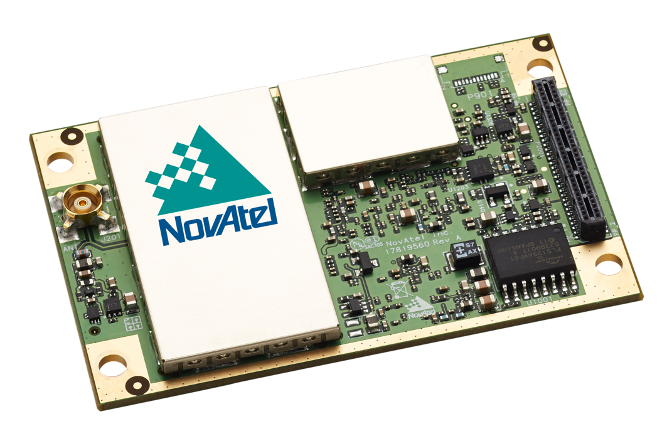
Hexagon | NovAtel
Hexagon | NovAtel is a prominent tech firm providing positioning, navigation and timing (PNT) solutions for multiple industry segments, including defense, surveying, construction, agriculture, autonomy and more. While GNSS is a core technology, NovAtel develops multi-sensor systems (including inertial) and has a broad reach with its OEM products. Surveyors, for instance, might not be familiar with NovAtel first-hand, but have likely used its technology via NovAtel’s many OEM customers.
Iain Webster
Iain Webster, senior director of Geomatics and Software Engineering for NovAtel, said that not only does NovAtel support high-rate RTK, but the customer can choose the position output rate desired — 1 Hz, 5 hz, 10 Hz, 20 Hz, etc. — and the receiver will output RTK positions at that rate.
“We distinguish between a matched solution (where a correction is matched with a rover observation at the same time tag), and a low-latency solution, where base observations are extrapolated for position computation at the rover,” Webster said. He provided a description from a company manual:
“The RTK system in the receiver provides two kinds of position solutions. The Matched RTK position is computed with buffered observations, so there is no error due to the extrapolation of base station measurements. This provides the highest accuracy solution possible at the expense of some latency, which is affected primarily by the speed of the differential data link. The MATCHEDPOS log contains the matched RTK solution and can be generated for each processed set of base station observations.
The Low-Latency RTK position is computed from the latest local observations and extrapolated base station observations. This supplies a valid RTK position with the lowest latency possible at the expense of some accuracy. The degradation in accuracy is reflected in the standard deviation. The amount of time that the base station observations are extrapolated is in the “differential age” field of the position log. The Low-Latency RTK system extrapolates for 60 seconds. The RTKPOS log contains the Low-Latency RTK position when valid, and an “invalid” status when a Low-Latency RTK solution could not be computed. The BESTPOS log contains either the low-latency RTK, PPP or pseudo range-based position, whichever has the smallest standard deviation.”
NovAtel does not brand this as a specific feature — it is just a standard part of its RTK solutions, but the company refers to it in their documentation as a “low-latency” solution.
The main benefit of this solution, Webster explained, is for kinematic users to allow better representation of their actual trajectory (such as in applications on moving vehicles). “The higher the dynamics, the more impact the latency of the matched solution will have to the point that we recommend the low-latency solution to all but specialist customers with known static positioning needs. For surveyors, there may be improved workflow with the low-latency solution as they will be able to move from point to point more quickly.”
NovAtel produces GNSS and inertial hardware and software, including OEM boards, for multiple applications. (Photo: NovAtel)
Webster noted that for applications where the rover is static for observations, 1 Hz can be fine, but for moving rover applications — kinematic — running at 1 Hz is probably unacceptable, so low latency is quite standard.
Additionally, he pointed out, there are applications where longer periods between corrections may not necessarily be detrimental. “Note that some manufacturers, including NovAtel and Leica, offer the possibility of using PPP corrections to extend RTK solutions beyond, for example, a 60-second timeout,” Webster said. “There are various proprietary methods to achieve this, but ultimately the RTK solution could be extended without limit in this way.”
Are there tradeoffs to using extrapolation or other high-rate approaches? “With corrections coming in at 1 Hz,” Webster said, “there is very little error over that period, so for most users, there is little disadvantage and perhaps some productivity advantage with a higher rate. If there is any trade-off, it is between getting the highest accuracy possible versus the lowest latency solution.”
As for the other scenario — the base broadcasting at greater than 1 Hz and the rover solving at greater than 1 Hz — “There is little advantage,” Webster said, “except in some specialized applications such as when the base is moving (called moving baseline) to provide a cm-level baseline between the base and the rover for relative positioning. For typical surveying applications with a static base, the rover would have to wait until the corrections arrived before outputting a solution. Other downsides include increased bandwidth on the communication link and more loading on the rover CPU, meaning lower battery life.”
What are the non-surveying applications where a high rate (in either scenario) can yield a specific benefit? Webster noted that, in fact, they deal mostly with non-surveying applications. “Most use cases need 10 Hz or 20 Hz for machine control or precision ag. We do have some very specialist applications that have required up to or beyond 100 Hz — but it is often best in those cases to do a GNSS/inertial navigation system (INS) solution and use the IMU to output at that a high rate. As previously mentioned, there are other specialist applications where the base is moving. In this case, we run a matched solution at a high rate between the base and the rover.”
Leica GeoSystems
With Xiaoguang Luo, Senior Product Engineer, GNSS Product Management Group
Rover with calibration-free tilt compensation and camera-based offset point capabilities. (Photo: Schrock)
Leica Geosystems (part of Hexagon) has been a major global developer and manufacturer of GNSS systems for multiple disciplines for several decades, introducing its first GPS receiver, WM101, in 1985. Since then, Leica has been among the leaders in GNSS receiver innovation, including integrated systems such as a rover that incorporates calibration-free tilt compensation and an image-point capture feature (GS18 I). Therefore, it is no surprise that for Leica Geosystems equipment features high-rate RTK as standard.
Xiaoguang Luo is a senior product engineer in the GNSS Product Management group at Leica Geosystems. He confirms that this option is supported in all Leica Geosystems RTK rovers of the current product portfolio, and this option is enabled by default in the Leica Captivate (surveying field) software. A term Leica Geosystems uses is prediction for its high-rate RTK approach.
Xiaoguang Luo
The standard positioning rate is 5 Hz on the rover. “As far as GNSS processing is concerned, there is no fundamental need to go to higher positioning rates,” Luo said. “The need for high rates is mainly driven by applications. For example, we are using the 5-Hz position update rate at the rover by default for an improved staking workflow and user experience. The 10-Hz rate is also supported in Captivate, for example, when streaming NMEA messages.” He added that 10 Hz is supported for other applications, such as structural monitoring, and 20 Hz for machine control.
As for the advantages of a rate higher than 1 Hz, Luo said that working at high observation and solution rates enables the possibility of modeling fast-changing error effects with a period below 1 second, and allows for high-rate non-surveying applications such as bridge monitoring. Does a high rate have any significant effect on the final results? He said that it strongly depends on the use case where high-rate observations and positions are involved. In addition, the quality of prediction also affects the final results.
Bernhard Richter
By this he means that while the standard approach for applications where the base is stationary, such as surveying, can work so well with a base data rate at 1 Hz and rover at 5 Hz, the key conditions do not change much over a single second.
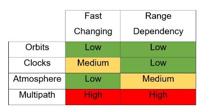
Luo’s colleague Bernhard Richter, vice president of geomatics, explained it. “To understand this, you need to separate the elements of corrections into those that are fast changing and range dependent (see the graphic below). If the errors change slowly, then they can be estimated and predicted very well. Or, if the range dependency is low, errors could come from a different source than the base station. If the range dependency is medium or high, then the corrections are more difficult to estimate on the rover side, but if such errors change very slowly, they can still be predicted very well with the precondition that corrections have been received at least once.”
The rate of change and dependencies for the elements of corrections. (Source: Leica GeoSystems)
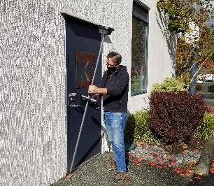
You’ll notice that multipath is high in both regards. This brings up another misconception about high-rate RTK — some users have an expectation that it will improve their performance in limited sky-view situations (like thick tree canopy) or high multipath environments. This is not so. Any improvements in such environments come from having more satellites, more observations, and more modernized signals. With regard to high-rate and multipath, Richter said, “It is anyway futile, since multipath decorrelates so quickly that the advanced mitigation has to happen both in an analog and a digital way on the rover.”
While there are benefits to running at high rate, such as for staking, a balance has to be struck — for instance, in not running it at too high a rate. Luo outlined disadvantages that must be considered when performing high-rate RTK.
High processing load and battery drain, particularly with multi-constellation and multi-frequency RTK.
High temporal correlations between observations, which may not be considered in a sophisticated manner in the RTK algorithms.
High base rates provide challenges for the RTK data link devices, such as radios.
In addition, he noted that while any kind of predictive solution will introduce some amount of error, that would be so small in, for instance, a base data rate at 1 Hz and rover at 5 Hz solution, as to not even be noticeable in the positioning results.
Septentrio
With Bruno Bougard, Research and Development Director
Bruno Bougard
“Our rover solution computes RTK up to 100 Hz,” said Bruno Bougard, R&D director at Septentrio. “Update rate requirements for industrial machine control applications are typically 20 Hz. This is necessary to capture the motion dynamics. Also, it is not only the update rate that matters in those applications, but also the latency, which should be low (<20 ms typically) and constant.”
Septentrio NV is a designer and manufacturer of high-end multi-frequency GNSS receivers and integrated solutions. Markets they serve include surveying, mapping, construction, science, timing, agriculture, marine, autonomy, and more — all with specific applications where high-rate RTK may be employed They also provide OEM boards and modules for further integration by others.
Surveying users for instance may be familiar with their Altus line of rovers, such as the NR3, where high rate is a standard option. “There are new applications where a higher update rate is required,” said Bougard. “Surveying with UAV, using photogrammetry or lidar scanning requires at least 10Hz. In mobile mapping in general, RTK-INS solutions such as SPAN, Applanix or Septentrio SBi, require update rates up to 200Hz.”
Bougard acknowledged that manufacturers use many terms for their high-rate solutions. “Some may be used to masquerading a low-rate solution as a high-rate one. This is not what we do. The rover observables are captured at high rate and can be up to 100 Hz. The rover RTK filter is also run on high rate. Fixed base-station data does not have to be high rate. 1 Hz is typically enough. For moving base applications — for example, when the base station is on another vehicle, and we want to compute the baseline between the moving base and the rover — 10 Hz is required.”
Bougard said that the benefit is to track the motion of the rover. This is critical in machine control, but also relevant for new survey flows (such as UAV-based and mobile mapping). The disadvantage, he explained, is that it requires higher CPU loads. “Suppliers, who focus on cost, tend to compromise on this, notably running higher rate only for a subset of the constellation or signals. We use them all.”
Is running the base station at a higher rate advantageous? “It is possible to increase the output rate of our base station correction stream but, as explained, this is not needed if the base is static,” Bougard said. “This is applicable to moving base scenarios as explained above. Indeed, if you increase the base-station correction rate, the bottleneck becomes the datalink.”
Tersus GNSS
With Xiaohua Wen, Founder and CEO, Tersus GNSS
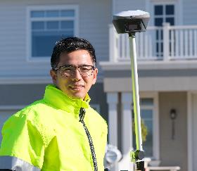
Xiaohua Wen with a Tersus GNSS receiver.
Xiaohua Wen, based in Melbourne Australia, is the founder and CEO of Tersus GNSS, another new entrant in the centimeter-grade GNSS market. One distinction about Tersus is that the company has developed and produces its own GNSS boards, instead of using OEM boards from other companies. Tersus implements its own tech, including GNSS receivers and IMUs in its own survey rovers, such as the Oscar, and for other high-precision applications. Additionally, it produces OEM boards for integration by others. Tersus entered the market with full multi-constellation support and, of course, high-rate RTK options, and has recently announced a PPP (precise point positioning) service.
“Our RTK boards support up to 20 Hz,” said Wen. “Often, surveyor will choose 5 Hz. We do a 5-Hz solution in this manner: the baseband takes raw measurements at a wanted moment, say at 1.2 s or 1.4 s, and RTK calculates solutions with the raw measurements. We understand that some older solutions might simply extrapolate or interpolate based on a position and velocity sequence, which is sometimes called predicted RTK or extrapolated RTK (though those terms get used in different ways by different developers). That is not how we approach our RTK solution updates. All Tersus RTK boards also support a maximum 20 Hz raw measurements outputs.”
Multi-constellation rover with calibration-free tilt compensation. (Photo: Schrock)
We asked about some of the advantages users may envision of high-rate RTK in general. Wen said there may be little or no gain with regard to faster initializations. Likewise, there is no significant gain with precision and accuracy. However, Wen said that higher rates can sometimes improve staking workflows. “For example, in the case of our Oscar rover with tilt compensation, the RTK outputs solutions at 10 Hz, while the IMU samples at 100 Hz. Oscar calculates the pole tip’s position at 10 Hz, aligned with the RTK solutions, and the data controller or tablet displays the point of the pole tip on the screen. We find that the point better refreshes at 2 Hz or higher to respond to the pole tip movements without noticeable lagging.”
That movement is an example of a key value of high rate,“Speed or movement,” Wen said. “For surveying applications, I would say that 1 Hz could suffice, considering the characteristic very low speed. Usually, applications like machine control and precision agriculture require an RTK update rate at 5 Hz or higher. Some UAV applications may use a 100-Hz position update. Most of these applications use an INS+RTK solution. With INS, it’s easy to get a 100-Hz position update, while for an RTK solution, a rate of 20 Hz is probably enough.”
Wen said that broadcasting corrections at a higher rate is pointless for most applications, “because the base data is highly correlated in the short term. If it’s a moving base, the high-rate base data would make some sense. Otherwise, it just imposes a greater load on communications and computation, with almost no gain.”
Topcon Positioning Systems
With Alok Srivastava, Director of Product Management
Alok Srivastava
“It is a standard option in our rovers,” said Alok Srivastava, senior director of Product Management (PM) at Topcon. “Around the time I joined the PM team, in 2010, the decision was made to make 10 Hz the standard, though this is user configurable and can be 5 Hz, 20 Hz, up to 100 Hz.” He explained that faster rates have been available through several generations of their receivers.
Typical applications consist of a static base and a moving rover. Fast-moving applications can benefit from higher rover position update rates since the RTK engine is computing real positions at a faster rate. Higher rates on the rover side provide accurate changes in position that can be missed by interpolating between positions computed at a slower rate.
A Topcon multi-constellation rover with tilt compensation. (Photo: Schrock)
High update rates on a base station do not provide advantages except in rare cases where the base is moving. While rovers are computing movements of the rover antenna, base stations are providing GNSS satellite corrections. A rate of more than 1 Hz for a static base station does not benefit rover accuracy; it only creates a burden on the communication between base and rover. Base and rover communication needs to be optimized to reduce bandwidth requirements. This is especially true as we continue to add constellations and signals to GNSS solutions.
Sufficiently high rates have been standard on Topcon rovers for a long time. Srivastava would rather see more focus put on other aspects of GNSS — such as interference, spoofing, the impacts of 5G, precise point positioning (which Topcon provides through its Topnet Live service) and sensor integration. “In many of our construction applications, we have IMUs,” Srivastava said. “When an application has an IMU for tilt compensation or for machine control, the IMU and GNSS complement each other. In kinematic mode, the IMU can help reject outliers.”
“High rate can be considered a common default mode of operation,” said Stuart Riley, vice president, Technology – GNSS, Trimble. “Typical rover position solution rates are 5 Hz, 10 Hz and 20 Hz.”
Trimble is one of the pioneering companies in GPS and GNSS, and Riley has been directly involved in the evolution of the company’s GNSS solutions for more than two decades. He has seen a lot of change, and in noting the nature of key technological advances, offered this intriguing observation about high rate: in many ways it has become less relevant.
“There have been considerable advances in RTK technology in recent years that make many of the earlier concepts related to how base and rover data should be combined for baseline processing largely irrelevant,” said Riley. “Most recently, survey receivers have included INS support for tilt compensation applications, and these receivers have available high-rate IMU data — at a much higher rate than GNSS observables — which drive the final GNSS/INS integrated solution. Thus, the rover GNSS data rate is not so important.”
Riley noted another relevant technology that Trimble has implemented: the use of precise satellite clock and orbit corrections — such as from the Trimble RTX precise point positioning (PPP) service — to augment RTK when there is a loss of the base correction stream. The implementation of PPP is broadening across the industry, and the company was an early implementer of a global service. It has the RTX-based xFIll feature that runs on and high-end survey receivers. One of the misconceptions about PPP services such as xFill is that it is just there to “take over” should the RTK or NRTK corrections be interrupted. Yes, it does that as well, but to be able to do that, it is running all the time, simultaneously with the RTK, so the rover is getting these enhanced PPP service clock, orbit and other data. This improves what the rover can do. “The emphasis in modern survey receivers,” Riley said, “is based more on the availability of rover data, and a fundamental base data rate of, say, 1 Hz, is all that is required.”
Along with various advances in the rover RTK engine, the GNSS constellations have expanded considerably, requiring increased bandwidth for the corrections from base to rover. “Our products can use various communication technologies to transmit corrections, such as Wi-Fi, cellular, and UHF (450 MHz or 900 MHz) radios,” Riley said. “Maintaining a 1-Hz correction rate enables all the GNSS observables to be broadcast from the base, providing a suitable highly compressed data format such as when Trimble’s proprietary CMRx format is selected.”
Many terms are used in the industry, and they typically refer to some proprietary aspect of an RTK engine. Riley said that a generic term would simply be high update rate. “Providing the position is based on the most current phase observables at the rover, a low latency solution is possible,” he said. “Thus low-latency solution goes hand-in-hand with a high update rate. Predicted RTK may refer to an old method where the static base corrections are propagated forwarded to account for radio latency and thus synchronize base/rover data. This is not used in modern PVT (position, velocity, time) RTK engines.”
High rate on the rover is standard, but what benefits should the user expect from it? “A fast update rate provides the best user interface experience in the field, in particular for stakeout,” Riley said. “Quite simply, nobody wants to be working with a laggy display. For survey field work, 5 Hz is typical. Other applications, such as machine control, benefit from higher update rates where a default of 10 Hz would be used, with options for higher rates.”
If the user chooses 1 Hz on the rover, what would be the downside? “Running at a 1-Hz rate is not really suitable for stake out,” Riley said. “For occupying static points, 1-Hz updates would suffice, as a typical occupation has a minimum time of 1 or 2 seconds. Very high rates for survey applications do not really buy anything in terms of field look and feel or performance.” I asked him about any points of diminishing returns, and he responded, “The higher the rate, the wider the measurement bandwidth (that is, the noise increases — you cannot get something for nothing), so in fact going for an unnecessarily high rate would start to be a disadvantage. For example, there would be no advantage to using a 50-Hz or 100-Hz rate for a land survey application. There is a relationship between measurement bandwidth and position noise.”
When is a high base rate a good idea? High rates are supported for some machine control and “moving base” applications where the reference frame has to move with the moving base, Riley said. In this case, the base and rover observables must be synchronized and the final solution has a fundamental latency depending on the base rate. For this reason, moving base rates are more typically 10 Hz or 20 Hz. For a static base, it is possible to use a higher rate. However, as Riley noted, “It’s more likely that a lower rate such as 0.5 Hz might be desirable to accommodate the radio when using repeaters (time multiplexing the data) or low data rates. There are disadvantages to high base rates, mostly related to radio bandwidth. Other factors, such as ‘high rate = more radio transmit power’, may need to be considered (affecting battery life).”
Are there other cases for even higher rover rates? “As mentioned, machine control applications use higher rates — necessary to reduce position latency in control loops,” Riley said. “Other applications such as UAVs and autonomous driving clearly benefit simply because of the speed of the platforms (higher dynamics). Precision agriculture is an excellent example of machine control, where auto guidance is used. Although high rates are possible, nearly all applications manage perfectly fine at rates up to 20 Hz. A more important consideration is system performance in terms of positioning accuracy and convergence times, which is dependent on the technology used in the PVT engine, such as Trimble ProPoint technology, rather than the correction stream data rate. ProPoint also includes xFill, as mentioned earlier, which provides centimeter-level backup for continuous operation when RTK or VRS correction streams are interrupted.”
Other Manufacturers
This was only a sampling of the developers and manufacturers, but it should be noted that several of the above firms produce OEM boards featured in dozens of other brands and models, such as Carlson and GeoMax. To try to list them all would be a challenge and might be missing a key point: high rate is quite standard, is not big news anymore, and you probably have it by default (or optional) no matter what system you are using.
Hypeful
As the insights the from industry experts above show: high rate can be essential for many applications, but unnecessary for others. It seems more about user experience (staking workflows or moving rover) than some way to seek higher precision.
Additionally, to borrow the gaming term hypeful, some users believe (or have been led to believe) that running at high rate will yield higher precision or work some kind of magic in dense tree cover or high multipath environments. Some may argue that it could get a result faster, but in practical terms even that might not be the case.
High rate has been around for a long time. And like any tech, has gone through different development and adoption phases. Think about automatic transmissions for motor vehicles; they have been around in one form or another for more than a century. There was a period in the mid-20th century where the development of different approaches was promoted in marketing campaigns with fanciful product names, like Durashift, Presto-Matic, Geartronic and Torque-Flite. But rarely do you see auto transmissions highlighted with such marketing flourish since then.
High-rate RTK was never singled out like that; it is common, and any differences are mostly in how it has been adapted for different applications. I suppose a firm could choose to emphasize it for marketing purposes and give it a buzz name like “Turbo Thrusted RTK”, which his fine for marketing purposes (albeit a bit “cheugy”). Every developer and manufacturer will have slightly different approaches, but if you believe, or are led to believe, that any represent high-rate fundamentals exclusively, that would be inadvertently misleading, if not subtle gaslighting.
As one of the experts said, “It does not really matter what manufacturers claim or don’t claim. You cannot beat physics. You can only understand and manage the physics.”
Coolness Ahead
While high-rate might seem a bit old hat, where GNSS development is going is not. The developers we interviewed are more interested in highlighting their complete high-precision solutions. For example, adding inertial measurement units (IMUs) for no-calibration tilt compensation, additional sensors for imaging (and likely soon, lidar), and multiple real-time GNSS solutions complimenting RTK, such as L-band precise point positioning (PPP).
The “high-rate” that is truly exciting is that of R&D, multi-sensor integration, automation of certain elements of workflows, artificial intelligence and multi-constellation/multi-signals.
TerraStar X corrections technology enables lane-level accuracy with under one-minute convergence for consumer and automotive-grade GNSS receivers
Hexagon’s Autonomy & Positioning division has partnered with Chinese positioning company Dayou to bring TerraStar X technology to the Chinese market. TerraStar X provides fast precise point positioning (PPP) corrections for autonomous vehicles and has mass-market use such as in smartphones.
The partnership enables Hexagon and Dayou to provide consistent positioning solutions globally, including North America, Europe and China, so original equipment manufacturers (OEMs) can deploy the same design worldwide.
The GNSS corrections generated from TerraStar X technology enable lane-level accuracy with convergence in under a minute for consumer and automotive-grade GNSS receivers, supporting advanced driver-assistance systems (ADAS), autonomous applications, safety-critical applications, mobile-phone applications and more.
TerraStar X technology delivers corrections using industry-standard formats compatible with mobile networks and enabling efficient delivery of corrections to millions of end-user devices. Through the partnership with Dayou, OEMs can now deploy the same high-accuracy solution across China as in North America and Europe, while having access to local sales, support and technical resources.
“This partnership provides a way for global companies to leverage TerraStar X technology to bring consistent lane-level positioning around the globe,” said Sara Masterson, director of positioning services at Hexagon’s Autonomy & Positioning division. “With its hardware-agnostic design, industry-standard format and delivery of corrections, this technology opens up the possibility of precise positioning for a multitude of new mass-market applications for customers to use one software positioning solution on all platforms worldwide.”
“Dayou is excited to be working with Hexagon in China to bring this next level of positioning technology to market,” said Han Jianxin, chief executive officer at Dayou. “High accuracy positioning used to be limited to expensive equipment and niche markets like survey and mapping. With TerraStar X technology, everyone can have the benefit of more accurate positioning, opening up new applications ranging from autonomous driving and freight to regular smartphone users moving from point A to B.”
Test Regions Expand to China
Using Dayou’s local infrastructure to calculate ionosphere corrections, TerraStar X technology ensures that fast convergence to lane-level and sub-meter accuracy is available when needed.
Engineering development test areas are available around the world to support large-scale programs with functional safety requirements. With these test regions now expanded to China, the partnership with Dayou marks a significant milestone to bring Hexagon’s TerraStar X technology to a global scale.
China Dayou PI is a Chinese company invested in by China Intelligent and Connected Vehicles (Beijing) Research Institute Co. Ltd. for high-precision positioning service and solutions based on GNSS, INS and HD map technology.
PUB QUIZ QUESTION:Who was Jean-Baptiste Alphonse Karr? He was a 19th-century French critic, journalist and novelist. He was at one time the editor of Le Figaro, the French daily newspaper. But he is most commonly known for the quotations from his works including the aphorism plus ça change, plus c’est la mêmechose commonly translated as “the more things change, the more they stay the same.” But what has this to do with GNSS you might ask?
One of the major sources of error in GNSS positioning is the ionosphere. As I have written in the Springer Handbook of GNSS, “[t]he ionosphere is that region of the Earth’s atmosphere in which ionizing radiation (principally from solar extreme ultraviolet (EUV) and x-ray emissions) cause electrons to exist in sufficient quantities to affect the propagation of radio waves. It extends from about 50 to 1000 km or more, above which we have the plasmasphere (also known as the protonosphere).” While GNSS technology has advanced over the years, Mother Nature stays pretty constant in the long term (global warming notwithstanding). And so the ionosphere is still a factor controlling the accuracy of single-frequency GNSS positioning as it has been for the past 40 years or more. The GPS navigation message includes values of the parameters of a simple ionospheric model known as the broadcast or Klobuchar model, named after its developer Jack Klobuchar. This model permits an estimate of the zenith ionospheric delay to be computed at a receiver’s location at a particular time of day and is driven by recent solar conditions as interpreted by the GPS control segment. The other GNSS use similar approaches in an attempt to reduce the positioning error of single-frequency positioning.
But the ionosphere is also an issue for dual- or multi-frequency positioning. Yes, the ionosphere is a dispersive medium so that by linearly combining simultaneous measurements (either pseudoranges or carrier phases) on two frequencies such as the GPS L1 and L2 frequencies, an observable virtually free of ionospheric effects can be constructed and used for position determinations. And high-accuracy positioning, particularly with carrier-phase observations, is possible with a relatively short period of observations using relative or differential positioning. However, the technique of precise point positioning or PPP requires tens of minutes or more of continuous carrier-phase observations to approach an accuracy level of a few centimeters — the well-known convergence problem of PPP. Back in 2014, Simon Banville, one of my former Ph.D. students, demonstrated that ionospheric corrections could be used to reduce the convergence time of PPP to 10-cm horizontal accuracies from about 30 minutes to a few minutes. This approach has drawn the attention of the positioning industry, which is looking into several aspects of its use including questions about the level of accuracy that can be achieved depending on the state of the ionosphere, the latency of corrections supplied in real-time PPP, as well as the location and coverage of the network of stations required to determine the corrections.
In this month’s article, researchers at Stanford University and Hexagon Positioning Intelligence team up to help answer these questions.
By Todd Walter, Juan Blanch, Lance de Groot and Laura Norman
Figure 1. The three station locations. (Image: Authors)
Hexagon is investigating the utility of applying ionospheric corrections to decrease the overall convergence time of the precise point positioning (PPP) filter. Stanford University has conducted several analyses on the accuracy of these ionospheric corrections over the course of the past two years. Stanford has created MATLAB tools to process data from multiple days and locations as well as to investigate intervals with larger disagreements between the raw ionospheric measurements and the provided corrections. In addition, the tool can apply varying magnitudes of latency to examine its effect on correction accuracy and error bounding.
The current study was performed using data from April 12–May 9, 2020. These days exhibit typical ionospheric behavior for a solar minimum period. Hexagon provided 1-Hz correction data for three International GNSS Service (IGS) sites to evaluate its accuracy:
Stanford University (IGS 4-letter identifier: STFU), 1-Hz data
Vandenberg Space Force Base (VNDP) in southern California, measurements at every 15 seconds
Priddis, Alberta, Canada (PRDS), measurements every 30 seconds.
These sites were chosen because they tend to have high volumes of good quality data and are covered by the ionospheric correction service.
The provided corrections were specifically calculated for the three selected reference sites. They include corrections for both GPS and GLONASS satellites. We downloaded RINEX data for the three sites for all 28 days from IGS. FIGURE 1 shows the locations of the three sites.
PROCESSING METHODOLOGY
The residual errors were determined by comparing the measured ionosphere to the corrections for all satellites. These differences contain a common mode effect due to the changing inter-frequency biases that are part of the corrections. We formed double differences for all satellite pairs (within each constellation) that have measurements and corrections present at the same time. For each such pair, the continuous tracks are determined, and a constant offset for each continuous track is subtracted to obtain the final residual error. This process is illustrated in the flowchart shown in FIGURE 2 as well as in the following example.
Figure 2. The processing flowchart. (Image: Authors)
FIGURE 3 shows the raw ionospheric measurements for GPS satellites with pseudorandom noise codes (PRNs) 3 and 31. The blue plus signs use the L2-frequency minus L1-frequency code-measurement difference divided by (γ–1) where γ is the square of the ratio of the L1 and L2 carrier frequencies (𝑓12/𝑓22≅1.65). The green circles are the L1 code minus the L1 carrier divided by two, and the red dots are the L1 minus L2 carrier measurement difference divided by (γ–1). The different measurements are formed to help identify erroneous measurements that might corrupt the evaluation. Fortunately, the vast majority of the measurement data is well behaved. The traces shown in Figure 3 are all self-consistent and indicative of valid measurement data. The carrier-phase difference measurements are then used in the remainder of the processing, as these have the least amount of measurement noise.
Figure 3 Raw ionospheric measurements for GPS PRNs 03 (left) and 31 (right). (Image: Authors)
On the left side of FIGURE 4, we present the carrier phase ionospheric delay measurements of PRNs 3 and 31 alongside their corresponding corrections. The middle section of the figure shows the differences between measured and estimated correction values for each satellite. Notice that there are common mode drifts that span ~50 centimeters for this example. The right side of Figure 4 shows the difference between the two curves in the middle portion. This double difference is the difference between these two corrected satellites for the periods of time that they are simultaneously observed by each reference station. For each continuous double-difference track (that is, it has no detected bias break), we subtract the mean value (provided that the track spans at least four minutes). We examine this residual error in meters and the normalized residual error where we divide by the root-sum-square of the provided correction 1σ values. The process begins by comparing PRNs 1 and 2, then comparing PRNs 1 and 3 and so on until PRN 31 has been compared to PRN 32. We then repeat the same process for the GLONASS PRNs.
Figure 4. Ionospheric measurements and corrections for GPS PRNs 3 and 31 (left), differences between the measurements and corrections (middle) and double differences between the satellite pair (right). (Image: Authors)
These values are put into histograms, and the 95%, 99.9% and 99.999% quantiles are determined for each metric. These are calculated on a daily basis across all satellite pairs as well as aggregated over multiple days and stations. By comparing different quantile behaviors, we can see whether the full distributions are close to Gaussian (well behaved) or if they have outliers that create large tail values (poorly behaved). FIGURE 5 shows the histograms of data for the Stanford University station for the first day analyzed.
Figure 5. Histogram of double-differenced residual error at Stanford (left) and normalized error (right). (Image: Authors)
As can be seen, the data is very well behaved (the histograms are plotted on a semi-log scale to emphasize the performance of the tails). If the data strictly followed a Gaussian distribution, we would expect that about 95% of the values would fall within 2σ, 99.9% within 3.29σ, and 99.999% within 4.42σ where σ is the standard deviation of the distribution. Often, similar data would have much wider tails and include many outliers; however, this data has only slightly wider tails than would be expected for a Gaussian distribution. The double difference includes the noise from two sets of measurements and two different corrections. The values in the right side of Figure 5 should be divided by the square root of 2 to assess the magnitude of error affecting just one satellite. The values on the left histogram use the square root of the sum of the variances associated with the corrections, so no similar adjustment is required there.
FIGURE 6 shows the results of evaluating the Stanford station over all 28 days. Here the 95%, 99.9%, 99.999% and maximum values are shown for each individual day. The 95% values are fairly consistent over the 28-day period, but there is more variability in the tails of these distributions. The same data was analyzed for Vandenberg and for Priddis. The errors are largest for Vandenberg, which is situated near the edge of coverage for the corrections, with a maximum value above 35 centimeters. Priddis has the smallest errors with a maximum value below 20 centimeters, likely due to good network coverage and smaller ionospheric delays nearer to the Earth’s polar regions.
Figure 6. Ionospheric corrections accuracy quantiles for GPS and GLONASS at Stanford April 12–May 9, 2020. Ionospheric delay double-differenced residuals (left) and normalized values (right). (Image: Authors)
FIGURE 7 shows the aggregate histograms for all of the data across the three stations for the full 28 days. Note that the84-days reference in the figure headers refers to station-days (28 × 3). The accuracy of these corrections for the vast majority of the data remains quite impressive; the 95% value indicates a 1σ accuracy of ~1 centimeters (3 centimeters/(2√2)). The higher quantiles indicate slightly larger values due to the wider tails of the distribution with the 99.9% indicating a 1σ of ~1.7 centimeters (8 centimeters/(3.29√2)) and the 99.999% indicating a 1σ of ~2.9 centimeters (18 centimeters/(4.42√2)). The provided error bounds are conservative for most of the data. For 95% they are four times larger than necessary, and for 99.9% two times larger. However, by 99.999%, they are only 10% larger than strictly necessary and are insufficient for even smaller probabilities. This highlights the larger tail behavior and that the error bounds, which are currently only a function of elevation angle, should be updated to reflect more information about the transformation of the reference measurements into the estimate of ionospheric delay. Corrections near to the edge of coverage or that make use of fewer or less accurate measurements would be expected to have larger error bounds.
Figure 7. Ionospheric correction histograms for GPS and GLONASS at all three sites April 12–May 9, 2020. Ionospheric delay double-differenced residuals (left) and normalized values (right). (Image: Authors)
KLOBUCHAR CORRECTIONS
We are currently at a solar minimum period, and the ionospheric delays are both smaller and smoother than are typically experienced during other phases of the ionospheric solar cycle. To demonstrate that the corrections are accurately following the ionospheric behavior, and that the demonstrated accuracy is not merely a reflection of an extremely smooth ionosphere, we repeated the same process using the single-frequency global ionospheric model broadcast by the GPS satellites. This model is commonly referred to as the Klobuchar model after its developer. FIGURE 8 uses the same measurement data as Figure 7, but now the corrections are replaced with the Klobuchar model from each day and the error bound is set to a constant 1 meter 1σ value. As can be seen, the error magnitude is significantly increased to values of 50–60 centimeters 1σ. Thus, the provided corrections are accurately following the ionospheric behavior to within a few centimeters, and the actual variations in the ionosphere are more than an order of magnitude larger.
Figure 8. Klobuchar correction histograms for GPS and GLONASS at all three sites April 12–May 9, 2020. Ionospheric delay double-differenced residuals (left) and normalized values (right). (Image: Authors)
To examine the changes in ionospheric variability over the solar cycle, we examined four eastern stations during a significant ionospheric disturbance on Oct. 29, 2003. These stations are in Bermuda; Greenbelt, Maryland; Santiago de Cuba, Cuba; and Washington, D.C. They experienced very large ionospheric gradients during that event. FIGURE 9 shows similar data for the four stations from that day. Note that, again, the figure headers refer to station-days and the x-axis for each graph had to be expanded to include all the errors. Here the errors are between 2.8 and 7.4 meters 1σ.
Figure 9. Klobuchar correction histograms for GPS and GLONASS at four sites on Oct. 29, 2003. Ionospheric delay double-differenced residuals (left) and normalized values (right). (Image: Authors)Ionospheric delay double-differenced residuals (left) and normalized values (right).
EFFECTS OF LATENCY
We are able to configure the tool to implement different levels of latency for the corrections. This is configured as a minimum age for the corrections before they can be applied to the measurements. In all cases, the maximum age of the data beyond the initial latency value was set to 30 seconds. For example, when set to 60 seconds of latency, corrections had to be at least 60 seconds old to apply to the current epoch. If no correction existed that was between 60 and 90 seconds old, then the measurement would not be corrected.
FIGURES 10 and 11 show results for this latency study. The top row of each corresponds to 0, 30 and 60 seconds from left to right. There was surprisingly little effect for this range of latencies, most likely due to the benign ionosphere during the current solar minimum period. The accuracy quantiles increased only by less than half of a centimeter over this period. The normalized errors saw somewhat larger growth, but the sigma values are still appropriately bounding the errors. The bottom rows correspond to 120, 240 and 360 seconds of latency, from left to right. Here we begin to see more effect from latency; the residual error is doubled by 360 seconds. Between 240 and 360 seconds, the 99.999% normalized residual error exceeds 4.42, which corresponds to the expected Gaussian value. We can also see more outliers beyond 6σ.
Figure 10. Histograms showing the double-difference residual accuracy for differing amounts of latency. (From left) Top row: 0, 30 and 60 seconds. Bottom row: 120, 240 and 360 seconds.
Figure 11. Histograms showing the normalized double-difference residual accuracy for differing amounts of latency. (From left) Top row: 0, 30 and 60 seconds. Bottom row: 120, 240 and 360 seconds.Bottom row: 120, 240 and 360 seconds. (Image: Authors)
We fit the quantiles vs. the latency times and found a strong quadratic dependence. TABLE 1 shows the resulting growth rates for the overall error and the 1σ values for each quantile. For the observed level of ionospheric activity, we recommend adding an increase to the 1σ confidence value as a function of the age of the correction. We recommend an added value of 4.5 × 10⁻⁵ centimeters/second2; thus, after 200 seconds, the 1σ value should be increased by 1.8 centimeters. However, for solar maximum periods and during significant ionospheric disturbances, we feel that this error bound will need to be increased, perhaps significantly. This error-bound term should be linked to the state of the ionosphere.
The correction accuracy is generally quite good, with 95% daily values almost always below 4 centimeters and below 6.25 centimeters overall. There are, however, outliers that affect the daily 99.9% and 99.999% percentiles, particularly at Vandenberg, which is toward the edge of the correction coverage region. The provided error bounds are mostly conservative, but there were still some occasional outliers. These error bounds should be more than simply functions of elevation angles. They should include real-time updates on the state of the ionosphere and quality of the correction based on the input measurements.
We evaluated the effects of latency and found that during this solar minimum period, fairly long latency times (up to 120 seconds) showed little impact on performance. It was not until more than 240 seconds that the sigma values stopped adequately bounding the tails and the overall accuracy degraded appreciably. We advocate including a quadratic term to the error bound to account for the age of the correction. During solar minimum time, we observed that this term can be quite small (4.5 × 10⁻⁵ centimeters/second2), but anticipate it needing to be significantly larger during times of ionospheric disturbance.
ACKNOWLEDGMENT
This article is based on the paper “Assessment of Ionospheric Correction Behavior for Use with Precise Point Positioning (PPP)” presented at the virtual 2021 International Technical Meeting of The Institute of Navigation, Jan. 25–28, 2021.
TODD WALTER is a research professor in the Department of Aeronautics and Astronautics at Stanford University. He received his Ph.D. in applied physics from Stanford in 1993.
JUAN BLANCH is a senior research engineer at Stanford University, where he works on integrity monitoring algorithms for radionavigation. He received a Ph.D. in aeronautics and astronautics from Stanford in 2003.
LANCE DE GROOT works for Hexagon Positioning Intelligence, Calgary, Alberta, Canada, in the Safety Critical Systems Group. He holds a B.Sc. and an M.Sc. in geomatics engineering from the University of Calgary.
LAURA NORMAN works for Hexagon Positioning Intelligence in the Safety Critical Systems Group. She obtained her B.Sc. and M.Sc. in geomatics engineering from the University of Calgary.
Every month, we ask members of our Editorial Advisory Board to weigh in on a topic. For the January 2021 issue, we asked,
Will precise point positioning (PPP) replace real-time kinematic (RTK)? If so, for which applications and when?
Miguel Amor
“Recently, Hexagon’s Autonomy & Positioning division demonstrated RTK levels of performance — globally —through PPP technology; we call it RTK From the Sky (see page 29). I believe that PPP adoption rates will grow significantly in the coming years and eventually replace RTK — especially in areas that are not well served by RTK networks or similar services. Adoption rates will depend on which applications can field GNSS receivers capable of the signals and constellations to perform like RTK.”
Miguel Amor Hexagon’s Autonomy & Positioning division
Alison Brown
“For many applications, the improved accuracy provided by PPP (10 cm) is sufficient and RTK solutions are not needed. However, the typical convergence time of PPP is between 20 and 40 minutes, depending on the number of satellites available, satellite geometry, the quality of the correction products, the receiver’s multipath environment, and atmospheric conditions. This slow convergence compared to RTK solutions will limit application for many real-time applications such as mobile solutions.”
Alison Brown NAVSYS Corporation
Jean-Marie Sleewaegen
“PPP-RTK combines near-RTK accuracy and quick initialization times with the broadcast nature of PPP, over internet or L-band. PPP-RTK can be seamlessly integrated into GNSS receivers, bringing convenient sub-decimeter accuracy to applications where configuring RTK is not practical or where there is no internet connection. PPP-RTK is likely to be adopted by emerging mass-market applications such as UAVs, while RTK will probably remain prevalent in applications where it is already well established, such as precision agriculture.”
Jean-Marie Sleewaegen Septentrio
Bernard Gruber
“I do not believe that PPP will replace RTK technology solutions anytime soon. Satellite-based GNSS correction services with an emphasis on global provide worldwide access, but achieving the required accuracy, due to convergence, can be slow. Today, myriad users and emerging customers may utilize corrections augmented with RTK transmitter/base stations that hybrid solutions can provide, thus solving both the age-old navigation issue of obscuration and near real-time positioning simultaneously.”
Antenna development, going all the way back to the first antennas, has been one of continuous innovation,” Richard Langley wrote in our September issue. Even after more than 30 years of GNSS technology development, he pointed out, GNSS antenna development continues.
His statement is borne out by the responses submitted by manufacturers of GNSS antennas to four questions we posed to them:
What specific challenges are your antennas designed to address?
Over the past three years and the next three years, what have been/will be your key innovations?
How are advances in real-time kinematic (RTK) and precise point positioning (PPP) changing requirements for GNSS antennas?
What technical challenges or industry trends do you find most interesting or noteworthy?
The responses display a wide range of antenna designs for a wide range of applications. They show how manufacturers must constantly balance requirements for positioning accuracy, form factor, interference management and cost. For the GNSS user segment, antennas are the first link in the processing chain and the first line of defense against jamming, spoofing, multipath and, increasingly, adjacent band interference. Antenna designers are also challenged by the growing adoption and sophistication of RTK, PPP and similar technologies. All these variables, challenges and scenarios are reasons for the constant evolution of GNSS antennas.
Finally, it is not always obvious whether a device should be classified as a receiver or an antenna. For example, what Harxon calls a “smart antenna” others might call a receiver.
Specific challenges
NovAtel antennas enable exceptional tracking for multi-constellation precision and are packaged for practical use in the field. Our antennas are designed to be the first link in the processing chain to deliver centimeter-level precision in harsh operating environments and applications, including contested or crowded RF environments through our CRPA antennas.
Key innovations
Over the past three years, we have focused on multi-frequency support and simultaneous L-band reception (seen in the NovAtel GNSS-850) to provide exceptional positioning solutions and support future technology like RTK From the Sky. Optimized to work with OEM7 receivers, NovAtel antennas leverage patented multi-point feeding networks to providΩe symmetric radiation patterns across all frequencies for excellent multipath rejection and minimal phase-center variation and offset. In the next three years, we expect to further reduce the size of antennas needed in a resilient high-precision solution. At the same time, we are continuing to improve robustness to adjacent band interference. We work to optimize the full GNSS ecosystem, from the signal in space reaching the antenna, to the final position, velocity and time (PVT) solution exiting the receiver.
Anechoic chamber testing. (Photo: NovAtel)
Advances in RTK and PPP
Advances in corrections expose measurements from low-quality antennas. You need an antenna with sub-millimeter phase-center variation (PCV) accuracy and stability on par with the algorithms delivering centimeter-level solutions. When the processing chain eliminates errors down to the centimeter level (or less), you must avoid adding errors from unstable phase centers, for example.
Technical challenges and industry trends
A difficult challenge facing the antenna industry is the commercial demand to reduce the size and weight of antennas while maintaining functionality and performance. The industry will need to continue balancing between size and performance while producing innovative GNSS antenna solutions integrated with other technologies, for example with anti-jam capabilities.
Harxon
With Leo Wang, Product Technical Director
Specific challenges
The design of Harxon’s GNSS antennas aims to achieve a perfect balance between easy integration with RTK solutions and the ultimate product performance by meticulously dealing with wideband, positioning accuracy, form factor, and interference management.
Key innovations
Over the past three years, our signature antenna innovation is our 4-in-1 X-Survey HX-CSX100A multifunctional GNSS antenna, which integrates a GNSS antenna, 4G, Bluetooth and Wi-Fi in one compact enclosure. This multifunctional antenna simplifies receiver integration into an RTK solution and facilitates industry development. In the next three years, Harxon looks forward to more breakthroughs in positioning technology and delivering pragmatic innovations.
Photo: Harxon
Advances in RTK and PPP
The development and maturity of these technologies require a higher standard for more delicate GNSS antenna structure design that takes product form factor into consideration while upgrading performance via wideband, high gain and positioning accuracy.
Technical challenges and industry trends
The 5G era has arrived, and the application of 5G technology for the internet of things (IoT) is extensive. China has also proposed the integration of 5G technology and BeiDou. We believe that, in the next few decades, GNSS positioning and 5G technology will be widely applied in the IoT industry and create huge benefits.
Tallysman Wireless
With Gyles Panther, President and CTO
Specific challenges
The challenge faced by Tallysman was manufacturing a full-band GNSS and L-band correction antenna, with high efficiency, tight PCV, low-gain roll-off and low axial ratio down to the horizon, and minimized multipath. Plus, a narrowly filtered low noise amplifier (LNA) to mitigate interference, all in the smallest possible package.
Key innovations
Over the past three years, Tallysman has released the VeraChoke, helical and VeroStar lines. The VeraChoke serves the geodetic and survey reference station markets with PCV and full-band GNSS coverage.
Our helical GNSS and Iridium antennas are lightweight, compact and robust. They provide a precise phase center and radically reduced dependence on a ground plane because of their differential mode of operation. Their exceptional low weight makes them an excellent choice for copter-style UAVs.
Photo: Tallysman
The patented VeroStar element combines full coverage of the upper and lower GNSS bands, plus L-band corrections service, with reception of L-band downlink Mobile Satellite Service (MSS) signals and exceptional low elevation angle reception. It is rugged, compact and lightweight — ideal for land and marine rover applications. It also provides minimal and symmetric PCV with outstanding all-around performance.
Advances in RTK and PPP
Both correction systems require rover receivers to phase-lock on low-amplitude GNSS satellite signal carriers, and both are hugely dependent upon the GNSS antenna. The corrections are critical for precision agriculture and land survey applications. Our precision antennas are specifically designed to minimize phase-lock loop (PLL) cycle slips.
Technical challenges and industry trends
Interference, accidental or intentional, is a major challenge and threat to GNSS, particularly from encroaching L-band 5G cellular systems. Tallysman offers tightly filtered LNAs and single-band omnidirectional anti-jam antennas with a deep null at low elevations. We plan to introduce a new multiband omnidirectional antijam antenna in the second quarter of 2021.
Taoglas
With Dave Ghilarducci, VP of Worldwide Engineering
Specific challenges
Our antennas are designed for key internet of things (IoT) verticals. Our high-precision, multi-band GNSS antennas offer centimeter-level positioning and timing accuracy for applications where small size and high performance are required. We address the industry’s most compact form factors with out-of-band rejection for operation near transmitters.
Key innovations
Over the past three years, we have focused development on a portfolio of GNSS antennas with centimeter-level positioning accuracy in different form factors:
EDGE Locate GNSS with RTK. (Photo: Taoglas)
lighter, more robust antennas through our patent-pending Terrablast-based products (the GGBTP.35); which are impact resistant and 35% lighter than traditional ceramic patches
high-rejection internal patch modules for rejection for OEM integrations (AGGBP.SL and AGGBP.SLS series)
surface-mount active patch antennas with embedded active circuitry for easier integration (ASGGB Simplicity series)
off-the-shelf module with an integrated multi-band RTK antenna, electronics and receiver technology for ease of integration.
Over the next three years, we expect to expand our portfolio and support additional bands like E6, L6 and the L-band correction band. Plus, we are working with the European Space Agency to design IoT devices with integrated high-precision RTK and GNSS technologies.
Advances in RTK and PPP
Expansion of RTK, PPP and similar technologies into new domains has demanded better performance from mainline and OEM antennas. These correction technologies stress antenna gain and polarization purity to maximize signal strength. We address these issues in our integrated designs to mitigate multipath errors and maximize ease of integration.
Technical challenges and industry trends
The release of lower-cost multi-band receivers and modules could be the most significant shift the GNSS industry has seen in the last decade. This innovation is already expanding applications and challenging suppliers to provide better performance for size, weight and cost.
Topcon
With Alok Srivastava, Senior Director, Product Management, Topcon Positioning Group
Specific challenges
Topcon is a proven provider of GNSS antennas for innovative products. Our GNSS product portfolio offers antennas with excellent multipath mitigation, near-band interference rejection, and quality signal tracking from zenith to the horizon. We strive to provide affordable solutions for our geodetic, machine control and agricultural customers.
Key innovations
Topcon antenna technology is applied within standalone antennas along with integrated GNSS receivers. Antennas inside our integrated receivers, such as the HiPer HR, are distinctive in supporting Bluetooth and Wi-Fi in a common antenna stack without sacrificing GNSS tracking and positioning performance. These offerings also support compact designs of integrated receivers.
As the number of GNSS constellations expands and new communication methods become available, potential inference from neighboring signals grows with congestion of the RF spectrum. Our standalone antennas, PN-A5 and CR-G5 with cavity filter option, uniquely address these challenges.
In the coming years, antenna technology will need to stay strongly focused on interference rejection and mitigation, lower cost and smaller size. These demands challenge antenna providers to make technical advancements while investing in cost-sensitive manufacturing along with higher testing standards. In this regard, our new antenna test facility in Concordia sulla Secchia, Italy, will soon be offering robotic calibration services.
Advances in RTK and PPP
With increased demand and services available for PPP, Topcon antennas support both GNSS and L-band frequencies, such as in the HiPer VR/HR receivers, and standalone antennas (PG-F1, G5-A1, PN-A5 and CR-G5). As data communications continue to expand beyond L-band and RTK/network RTK, Topcon systems will support them without compromising positioning performance.
Technical challenges and industry trends
As GNSS antennas are one of the integral items within the GNSS system, the significance of delivering a cost-effective and miniaturized solution that provides robust positioning is critical to meeting needs in ever-growing precise positioning markets and applications. Topcon will continue to emphasize innovative antenna products through our research.
Trimble
With Stuart Riley, Vice President of GNSS Technology
Specific challenges
Each application has different requirements. For applications that require the highest position accuracy, the stability of the phase center, multipath mitigation, and the unit-to-unit production consistency are critical.
Some markets require high performance, and often in challenging environments such as high vibration experienced on construction equipment. Other customers require smaller, lower cost antennas and can tolerate a slight accuracy reduction.
The antenna is typically a combination of a passive antenna element with an active low-noise amplifier (LNA). The LNA needs to be carefully designed to remain linear in the presence of in-band jamming while rejecting out-of-band signals.
Key Innovations
For high-precision applications, Trimble first released the Zephyr series of antennas in the late 1990s. This antenna provides excellent phase center stability and unit-to-unit production repeatability; the antenna has exceptional multipath mitigation performance, which is enhanced in the geodetic version.
Since the Zephyr was first introduced, we have added support for additional GNSS systems and RF bands (L1/E1, L2, L5/E5 and L6/E6), transitioned to a RoHS-compliant manufacturing process, improved the LNA performance, developed rugged versions for construction vehicle mounting, and produced a smaller version used in the Trimble R10, R12 and SPS986 GNSS receivers.
More recently, we developed a lower cost high-performance antenna for the Trimble Catalyst software-defined GNSS receiver for Android phones and tablets. We also introduced an antenna in the Nav-900 guidance controller for agriculture that implements a meta-material design.
Looking forward, we will continue to innovate by providing antennas optimized to meet the needs of the markets, including cost, performance and morphology. Enhancements will include novel antenna architectures, production technique improvements, and careful material selection.
Advances in RTK and PPP
Applications for GNSS are expanding to include more non-technical users, and the markets are calling for small, light and low-cost antennas — especially for technologies like PPP and positioning products such as Catalyst. These requirements extend across all arenas, especially in applications served by RTX. The needs must be balanced against increased technical demands stemming from the expansion in GNSS bands supporting new frequencies and signals, including PPP correction data.
Technical challenges and industry trends
The challenges come in balancing seemingly conflicting needs for performance, size, weight and cost for the various applications.
Because Trimble focuses on specific user segments, we can provide antenna solutions that are the best fit for the various applications. For example, an antenna in a handheld device must be small and lightweight; however, on a construction machine, durability takes precedence over size and weight.